the Creative Commons Attribution 4.0 License.
the Creative Commons Attribution 4.0 License.
 | 07 Nov 2018
On the role of thermal expansion and compression in large-scale atmospheric energy and mass transports
Melville E. Nicholls
Roger A. Pielke Sr.
There are currently two views of how atmospheric total energy transport is accomplished. The traditional view considers total energy as a quantity that is transported in an advective-like manner by the wind. The other considers that thermal expansion and the resultant compression of the surrounding air causes a transport of total energy in a wave-like manner at the speed of sound. This latter view emerged as the result of detailed analysis of fully compressible mesoscale model simulations that demonstrated considerable transfer of internal and gravitational potential energy at the speed of sound by Lamb waves. In this study, results are presented of idealized experiments with a fully compressible model designed to examine the large-scale transfers of total energy and mass when local heat sources are prescribed. For simplicity a Cartesian grid was used, there was a horizontally homogeneous and motionless initial state, and the simulations did not include moisture.
Three main experimental designs were employed. The first has a convective-storm-scale heat source and does not include the Coriolis force. The second experiment has a continent-scale heat source prescribed near the surface to represent surface heating and includes a constant Coriolis parameter. The third experiment has a cloud-cluster-scale heat source prescribed at the equator and includes a latitude-dependent Coriolis parameter. Results show considerable amounts of meridional total energy and mass transfer at the speed of sound. This suggests that the current theory of large-scale total energy transport is incomplete. It is noteworthy that comparison of simulations with and without thermally generated compression waves show that for a very large-scale heat source there are fairly small but nevertheless significant differences of the wind field.
These results raise important questions related to the mass constraints when calculating meridional energy transports, the use of semi-implicit time differencing in large-scale global models, and the use of the term “heat transfer” for total energy transfer.
- Article
(14757 KB) - Full-text XML
-
Supplement
(10199 KB) - BibTeX
- EndNote


Satellite studies of the zonally averaged top-of-atmosphere (TOA) radiative fluxes show that there is a net input of energy at low latitudes and output at high latitudes (e.g., Vonder Haar and Suomi, 1971). For a heat balance, there must be a poleward transfer of total energy, and fluid motions of both the atmosphere and oceans are considered to play major roles. It has been generally understood that the atmosphere and ocean carry heat from one area to another in an advective-like manner by the winds and ocean currents. However for the atmosphere this was brought into question by numerical modeling studies conducted with a fully compressible numerical model (Nicholls and Pielke, 1994a, b; hereafter NP94a and NP94b, respectively). It was found that large quantities of internal and gravitational potential energies could be transferred in a wave-like manner at the speed of sound. The basic idea is relatively straightforward: consider for instance that as an air parcel is heated it causes the temperature and pressure of the parcel to increase (a hot air balloon would be another way to think about this). The resultant pressure gradient between the heated air and its immediate environment then drives a divergent outflow causing the heated air parcel to expand. What is usually considered the salient point is that the expansion leads to a density decrease and therefore makes the air parcel (or hot air balloon) more buoyant. However, at the same time, the expansion of the air parcel must also cause the air in the immediate surroundings to become compressed, and that means the pressure must increase in this surrounding air. The pressure gradient therefore works outwards, continually accelerating air in an expanding radius. The result is the generation of a compression wave that we have termed a “thermal compression wave”, which has some clear similarities to a mechanically forced sound wave.
Thermal compression waves produced in this manner are not high-frequency sinusoidal waves so in this respect they differ from typical sound waves. There is a wavefront that propagates at the speed of sound and behind this a region of compressed air. It is at this point that it can be seen that a transfer of energy and mass might be occurring since compressed air has more molecules per unit volume and in the mean the molecules are moving slightly faster. The perturbations of pressure, temperature, and density in the large volume of compressed air surrounding the heated air parcel are extremely small compared to those occurring in the immediate vicinity of the air parcel where relatively strong buoyancy circulations develop. Nevertheless this rapidly widening envelope of compressed air with small internal energy and density anomalies adds up over a very large volume to constitute a major reservoir of total energy and mass, and this reservoir does not stay in place once the heating ends, but propagates away rapidly at the speed of sound.
While this theory of total energy transport has been known for some time it has not yet had any significant impact on the global-scale view of how total energy transport is occurring. In this paper one of the main objectives is to show that this mechanism of total energy transfer is likely to be important for large scales, and moreover to point out that this mechanism is probably not simulated very well in current global-scale models. For simplicity this study does not consider water substance. It utilizes an idealized framework, by looking at the transfers of energy and mass that occur in response to imposed heat sources in an initially quiescent atmosphere. Therefore it is difficult to draw definitive conclusions about how much energy and mass might be transferred by this mechanism in a more realistic large-scale atmospheric circulation that includes for instance the Hadley circulation, Rossby waves, and baroclinic eddies. This study extends on previous work by considering larger scales and the effects of including the Coriolis force. A comparison is made between simulations with and without thermally generated compression waves and it is demonstrated that differences start to become noticeable when the horizontal scale of the diabatic forcing is very large. Fields of vertically summed energies and mass are constructed to give a clear perspective of the lateral transports. Furthermore, the total heat input is calculated and compared to the total energy perturbation in the model domain to check energy conservation. Since the perturbations associated with thermally generated compression waves are typically extremely small it might seem at first sight that their effects can be safely neglected. The case is made that inaccuracies will be produced when they are not simulated correctly on the large scale, which might not be negligible.
The paper is organized in the following manner: Sect. 2 gives an overview of the two theories. Section 3 discusses the numerical model and Sect. 4 the design of the three experiment configurations, which consist of convective-scale, continent-scale, and cloud-cluster-scale simulations. Section 5 presents results for the three main experiments and several auxiliary experiments. In Sect. 6 the significance of these results for understanding total energy and mass transfers are discussed as well as potential implications for climate modeling. Finally in Sect. 7 conclusions are summarized.
2.1 The current paradigm of total energy transport
The derivation of the total energy equation can be found in many standard texts (e.g., Gill, 1982; Peixóto and Oort, 1992). It can be written in the following form:
where cv is the specific heat at constant volume, ρ the density, T the temperature, g the acceleration due to gravity, L the latent heat of condensation, q the specific humidity, u the velocity vector, p the pressure, F the radiative flux density, κ the thermal conductivity, and μ the viscosity. The total energy is comprised of internal energy, gravitational potential energy, latent heat energy, and kinetic energy. Note that this Eulerian conservation equation concerns the energy per unit volume.
In large-scale energy budget studies the hydrostatic approximation is made and the flux across a vertical latitudinal wall is rewritten in the (x, y, p) coordinate system (Priestley, 1949; White, 1951a, b; Starr and White, 1954). The following expression can be derived for the flux across a circle of latitude (e.g., Oort and Peixóto, 1983):
where the enthalpy has been introduced , cp is the specific heat at constant pressure, Re the radius of the Earth, ϕ the latitude, v the meridional velocity, and p0 the surface pressure. To derive this equation the terms involving kinetic energy, thermal diffusion, and viscosity have been neglected. Note that Eqs. (1) and (2) are often expressed as a time average. Oort and Peixóto (1983) make the following statement regarding the time average of the term on the right side of Eq. (2): “Further, the integrand can be decomposed into the contributions by transient eddies, stationary eddies, and mean meridional circulations in order to get a better understanding of the physical mechanisms involved in the fluxes”.
where overlines represent a time average and square brackets a zonal average. The prime symbol represents the departure of the variable from the time average and the asterisk the departure from the zonal average. A tacit assumption that is commonly made in interpreting Eq. (3) is that total energy is a quantity that is advected solely with the wind. For instance, the term is considered a transient eddy flux of enthalpy, implying that a large-scale eddy that moved warm air poleward and cold air equatorward would be physically accomplishing a meridional total energy transport. However, studies that have conducted detailed analyses of total energy transfer using fully compressible models demonstrate that total energy can be transferred in a wave-like manner at the speed of sound, which challenges this assumption (NP94a and b; Nicholls and Pielke, 2000). There is nothing intrinsically wrong with the decomposition in Eq. (3) and the transfer of energy by compression waves would be included. However, the assumption that total energy is transported in an advective manner may have led to practical methodologies for computing the contributions in Eq. (3) that do not account for the possibility of energy transport at the speed of sound. This issue will be discussed further in Sect. 6.
2.2 A linearized one-dimensional solution for a thermal compression wave
When an air parcel is heated the temperature and pressure increases and the resulting pressure gradient causes it to expand. During its expansion, the air surrounding the parcel is compressed. This compression does not simply remain in situ; a wavefront propagates away from the heated air parcel at the speed of sound, leading to weak positive pressure, temperature, and density anomalies over an increasingly large volume surrounding the heated air parcel. The internal energy per unit volume given by cvρT can be rewritten using the ideal gas law p=ρRT, where R is the gas constant for dry air, as cvp∕R. Therefore a positive pressure anomaly in the region of compressed air means that the internal energy is increased in this region. In addition, the increased density means that the gravitational potential energy ρgz is increased. Therefore this mechanism can quickly lead to an increase in total energy over a very large volume surrounding the air parcel and constitutes a total energy transfer at the speed of sound. NP94a derived a simple mathematical solution illustrating the basic process in the absence of the gravitational force for the one-dimensional linearized momentum, thermodynamic, and continuity equations which allow thermal compression waves. This solution, which has been expanded to include the temperature perturbation, is given in the Supplement (Sect. S1 and Figs. S1 and S2). Furthermore, expressions for the total energy and wave energy are given in Sect. S1 Eqs. (S6) and (S7) in the Supplement, respectively. Figure S3 compares the internal energy in a wave produced by a heat pulse with the wave energy.
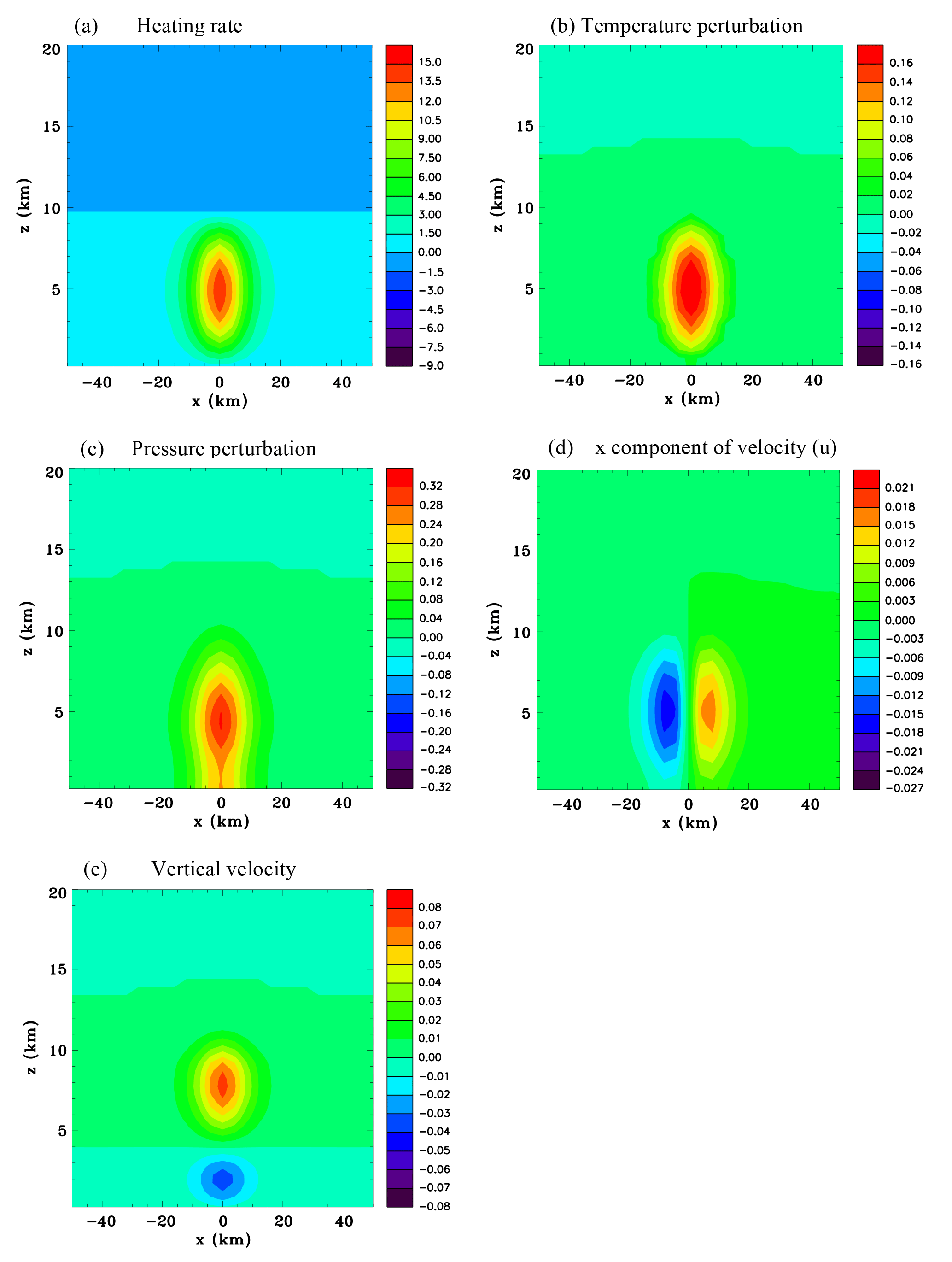
Figure 1Vertical sections for the convective-scale heat source, Experiment 1A, at t=10 s. (a) Heating rate (J kg−1 s−1), (b) temperature perturbation (K), (c) pressure perturbation (hPa), (d) x component of velocity (m s−1), and (e) vertical velocity (m s−1).
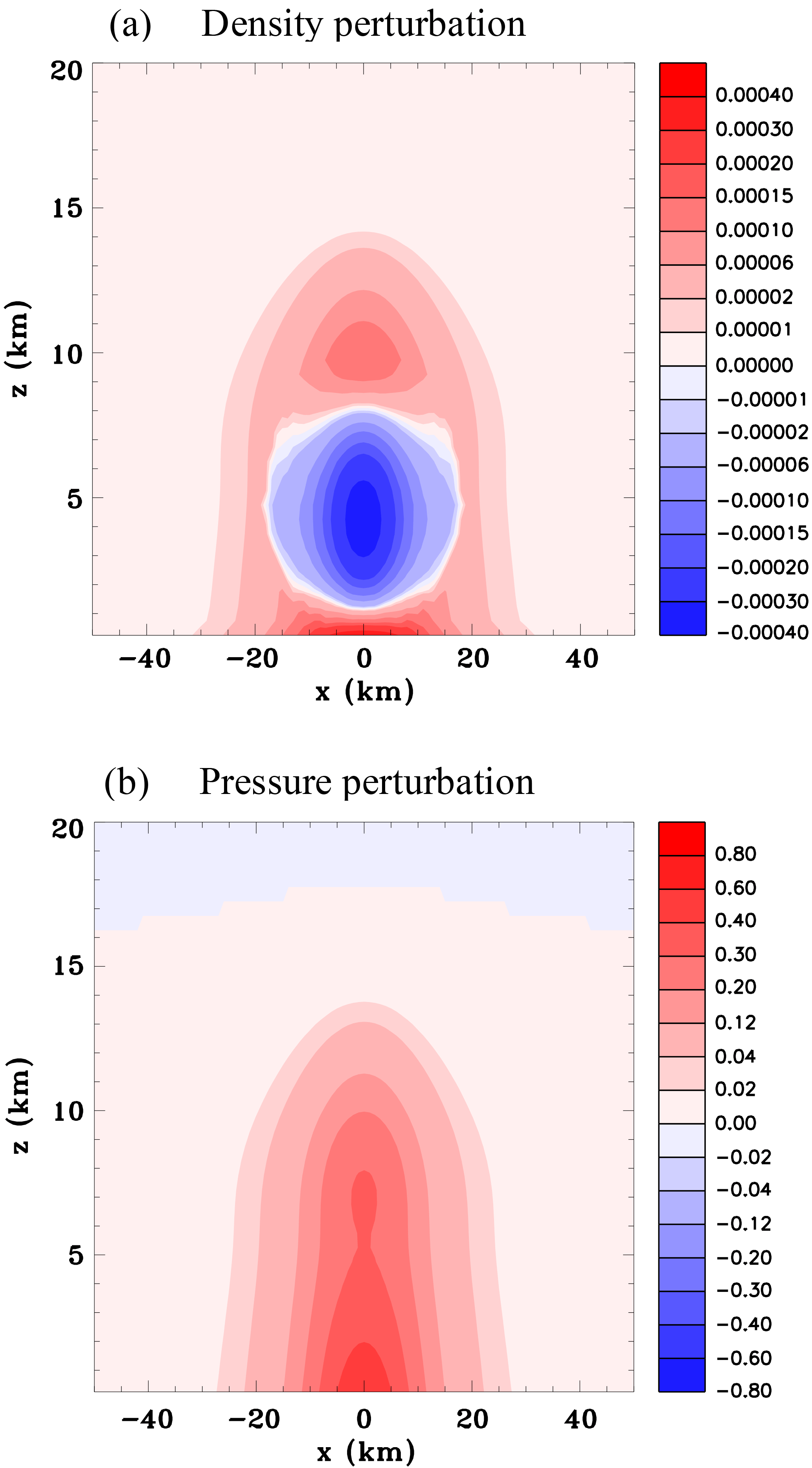
Figure 2Vertical sections for the convective-scale heat source, Experiment 1A, at t=20 s. (a) Density perturbation (kg m−3) and (b) pressure perturbation (hPa).
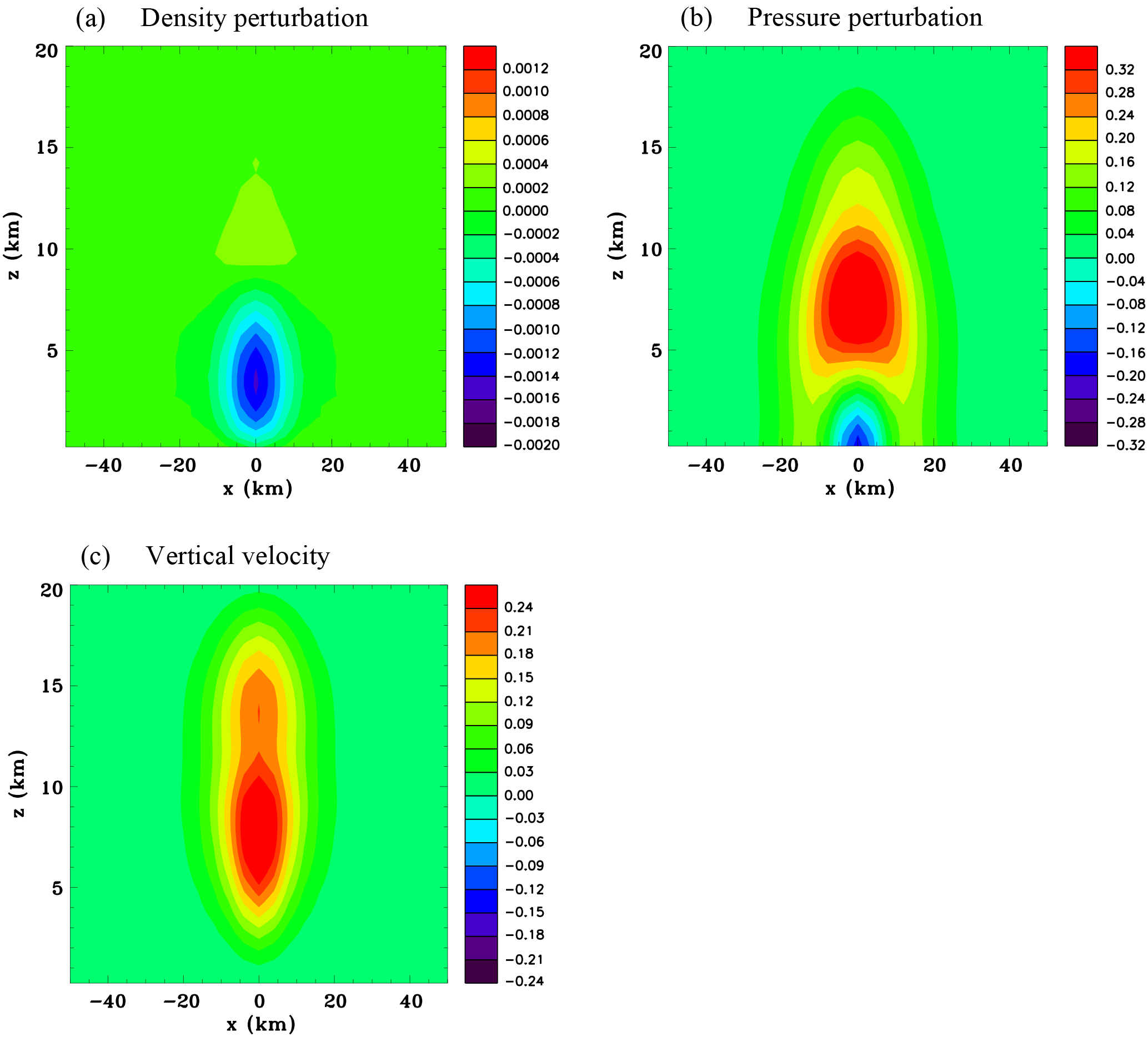
Figure 3Vertical sections for the convective-scale heat source, Experiment 1A, at t=40 s. (a) Density perturbation (kg m−3), (b) pressure perturbation (hPa), and (c) vertical velocity (m s−1).
The solution for a heat pulse having a duration of 600 s shows anomalies moving in opposite directions from the source region at the speed of sound (Fig. S2). The positive pressure perturbations indicate that these are regions with enhanced internal energy as shown in Fig. S3. While the central heated region has warmed considerably, there is no significant change in internal energy per unit volume. (cvρT) since there has been a large density decrease in the narrow heated region. Mass can be seen to be conserved since the density has increased slightly in the two wide compressed regions which are propagating away at the speed of sound. Therefore, this simple 1-D solution shows a significant redistribution of internal energy and mass occurring at the speed of sound.
The magnitude of the wave energy in the fast-moving anomaly for the heat pulse solution is 4 orders of magnitude less than the internal energy perturbation (Fig. S3). It is important not to confuse these two energy forms that can both be derived from the linearized equations.
2.3 A thought experiment demonstrating internal energy transfer is different than convective heat transfer
Another perspective on total energy transfer was presented in NP94b based on a thought experiment. A detailed description is provided in the Supplement (Sect. 2 and Fig. S4). An ideal gas in a container was considered that was divided by a movable frictionless partition. Heating the gas on one side of the container would cause it to expand and the gas on the other side to be compressed (Fig. S4). Considering a control volume within the unheated, side the compression would have resulted in an increase in internal energy. This increase would be identical to the increase in internal energy in a similar-sized control volume within the heated side since the pressure on both sides of the container would be identical and the internal energy per unit volume only depends on pressure. If the partition was removed and the gas stirred so that the warmer air was mixed with the relatively colder unheated air this would not result in a transfer of internal energy into the control volume on the right side of the container since the pressure would remain virtually unchanged.
Convective heat transfer is considered to be the transfer of heat from one place to another by the movement of fluids. It is common in meteorology to describe heat as being advected from one place to another, whereby it is meant that when relatively warm air moves into a region it constitutes a heat transfer. This interpretation is at the heart of the decomposition made in Eq. (3). From this perspective the heat transport in the thought experiment depicted in Fig. S4 took place in the second stage when air was mixed and the air in the control volume became notably warmer. However, this did not constitute a total energy transfer, which occurred earlier in the first stage during the compression of the unheated gas.
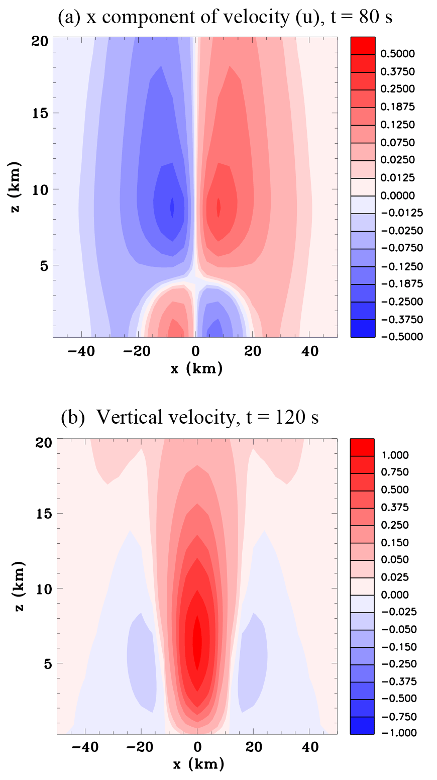
Figure 4Vertical sections for the convective-scale heat source, Experiment 1A. (a) x component of velocity (m s−1), at t=80 s; and (b) vertical velocity (m s−1), at t=120 s.
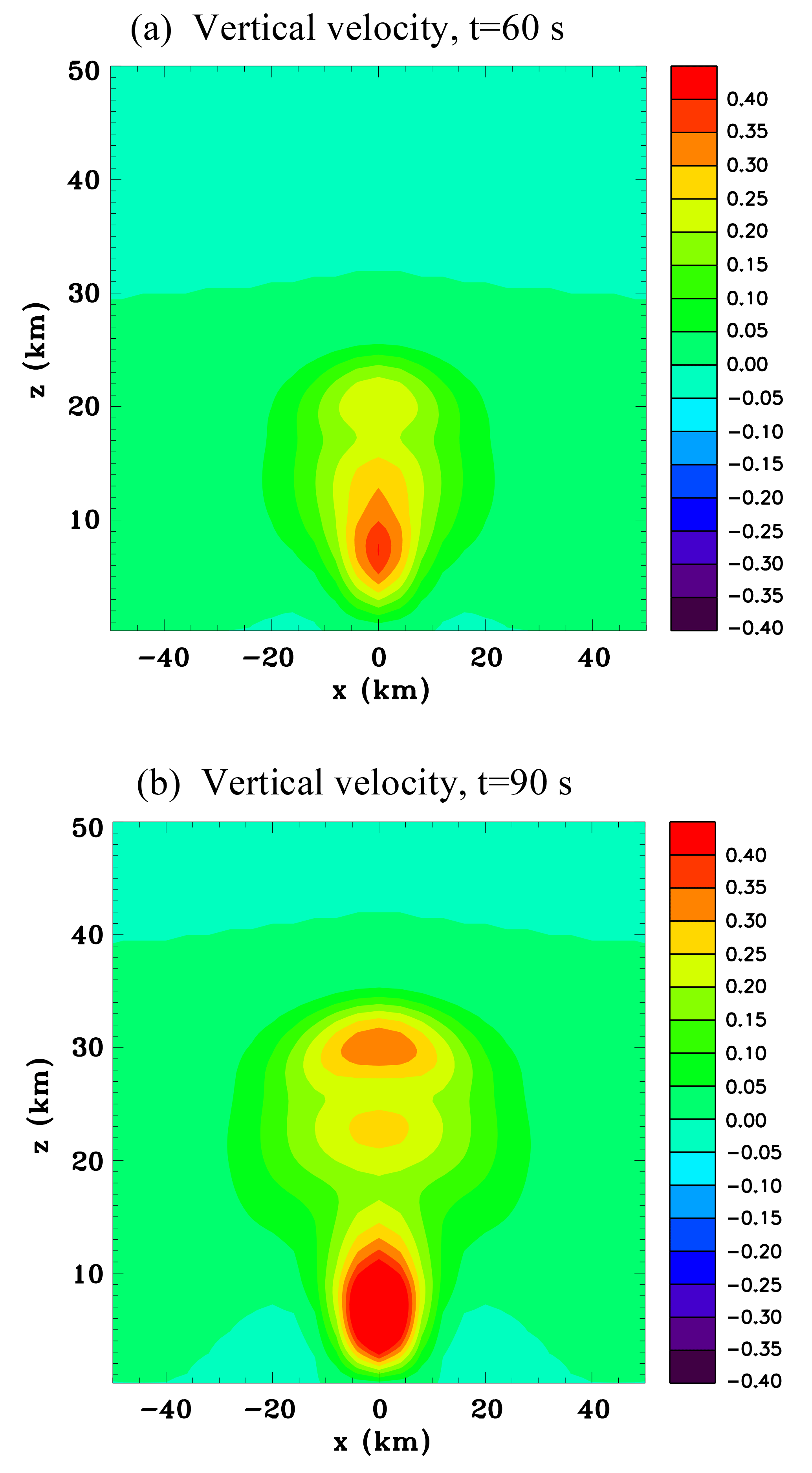
Figure 5Vertical sections for the convective-scale heat source, Experiment 1A. (a) Vertical velocity (m s−1), at t=60 s; and (b) vertical velocity (m s−1), at t=90 s.
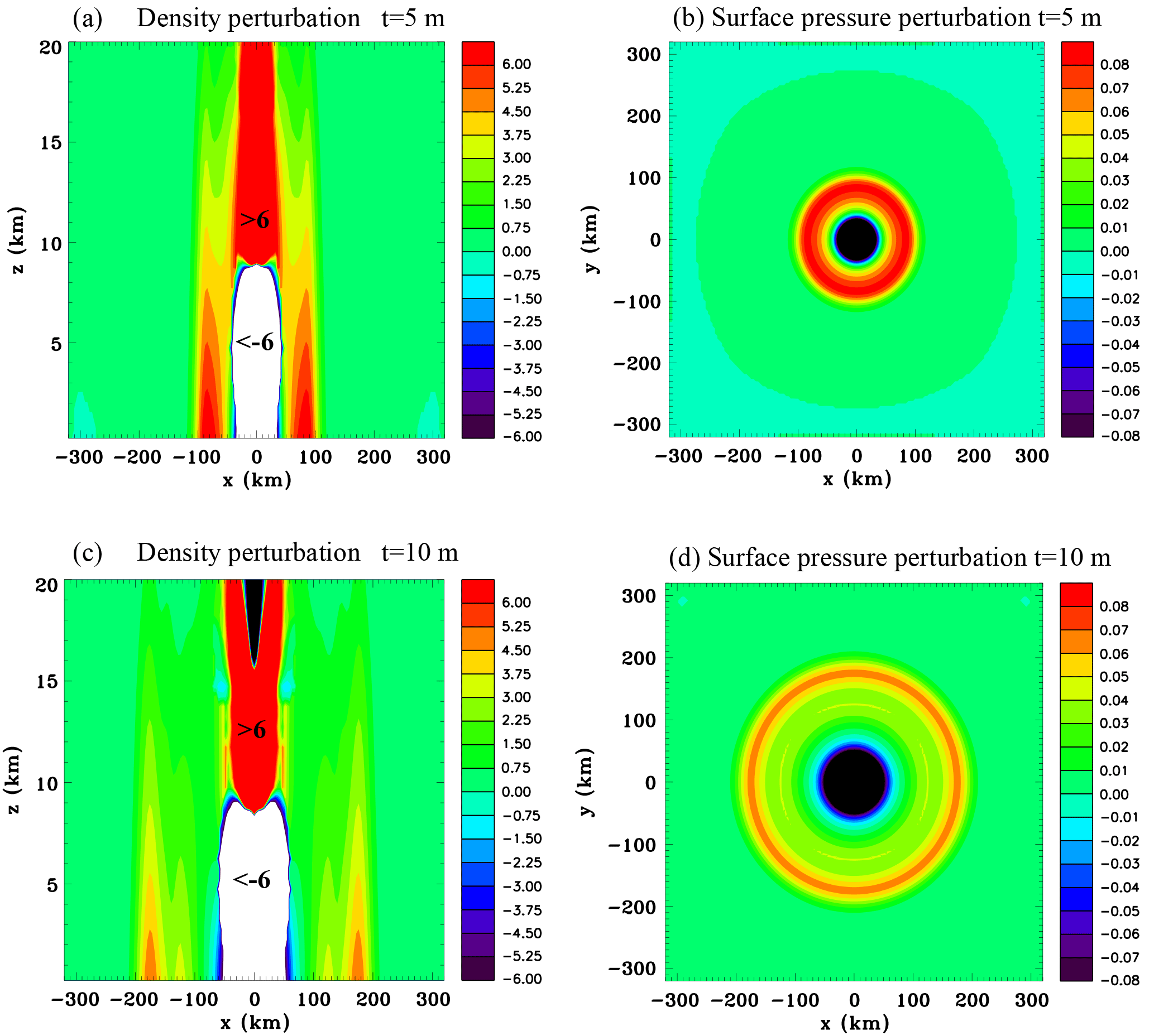
Figure 6Convective-scale heat source, Experiment 1A. Vertical sections of the density perturbation (kg m and surface pressure perturbation (hPa) at t=5 min (a, b) and at t=10 min (c, d).
The idea that convective heat transfer is not the same thing as internal energy transfer is a very simple idea as shown by this thought experiment and should not raise any red flags. Now take this one step further and propose a similar thing is actually happening in the atmosphere and that internal energy is being transferred at the speed of sound. This apparently is one step too far and this hypothesis becomes subject to incredulity.
2.4 Different meanings of heat transfer
It is pertinent at this stage to review three uses of the term heat transfer:
-
In thermodynamics, heat is defined as energy in transit across the boundary of a system, which does not involve work or the transfer of matter. Since heat is the flow of energy across the boundary of a system it is not correct to say it is stored in the system. However, the transfer of heat does lead to an increase in the internal energy of the system equal to the heat transferred.
-
Convective heat transfer within the body of a fluid is often defined as the transfer of heat from one place to another by the movement of fluid elements. A moving fluid element is said to carry energy with it. This energy is often described as thermal energy, or internal energy. However, there is a problem with this interpretation as made clear by the thought experiment discussed in Sect. 2.3. Transport of relatively warm air into the control volume during the mixing stage did not result in a change of the internal energy within the control volume. It led to a change in temperature, such that the mean kinetic energy of the molecules in the control volume increased, but their number decreased (corresponding to the density decreasing) so that overall there was no net change in internal energy.
-
The expression for the change of total energy (Eq. 1) involves fluxes of enthalpy, gravitational potential energy, and latent heat energy. These summed have also been called a “heat flux”.
Clearly the term “heat” is being used for different physical quantities, and this is one reason there is confusion on this issue.
Consider the thought experiment discussed in Sect. 2.3 and suppose that the warm and cold air in a thin region at their interface started to be mixed after removal of the partition. The turbulent eddies produced by the stirring should not result in a horizontal transfer of internal energy as we have maintained. Now consider putting a brief heat source at the far left side of the container, which produced a transient compression wave that proceeded to propagate through the interface between the warm and cold air that is being stirred. As the compression wave passes from left to right through the region of eddies there would for a brief instant of time be an enthalpy flux and internal energy would consequently increase on the far right side of the container. It would not be accurate to say that the turbulent eddies are physically responsible for that enthalpy flux just because they occupy the same space as the compression wave.
Obviously the exchange of warm and cold air masses in the container is of major physical importance as are the meridional transports of warm and cold air by eddies in the atmosphere. This meridional transport in the atmosphere is playing a significant role in the overall energy balance. For instance, TOA radiative fluxes would be different without these warm and cold air advections. However the simple thought experiment discussed above suggests that the quantity total energy in Eq. (1) is not necessarily being transferred when there is advection of warm or cold air masses. The transfer of the quantity total energy is complicated to understand because the atmosphere to a reasonable approximation behaves like an ideal gas so that heat input results in expansion and work being done on the surrounding air. This work done compressing the surrounding air is fundamental to understanding why energy is quickly redistributed at the speed of sound.
2.5 Vertical transport of total energy
Consider a horizontally homogeneous atmosphere and low-level heat source. The heated air will expand in the vertical and work will be done not only against the atmospheric pressure as in the example discussed in Sect. 2.2, but also against gravity. The acoustic cutoff period in the troposphere and stratosphere is approximately 5 min (Beer, 1974; Walterscheid et al., 2003). Shortly after the low-level heat source is turned on in a simulation an upward-propagating pulse of vertical velocity develops. This pulse propagates upwards at the speed of sound and increases in amplitude as it reaches higher levels (e.g., NP94b). When it reaches 100 km above the surface after traveling for approximately 5 min, a trailing lobe with negative vertical velocity becomes evident. If there is a Rayleigh friction layer at upper levels then the wave will not reflect off the top of the model. As the simulation continues further wave-like activity of the vertical velocity occurs, but its amplitude is relatively small in the troposphere and lower stratosphere, where persistent weak upward motion prevails. Walterscheid et al. (2003) discuss results of a model simulation of acoustic waves in the mesosphere and lower thermosphere generated by deep tropical convection. They found quite a complicated behavior with a trapped oscillation below about 80 km altitude with a period of ∼5 min and a nearly vertically propagating wave with about a 3 min period above this height.
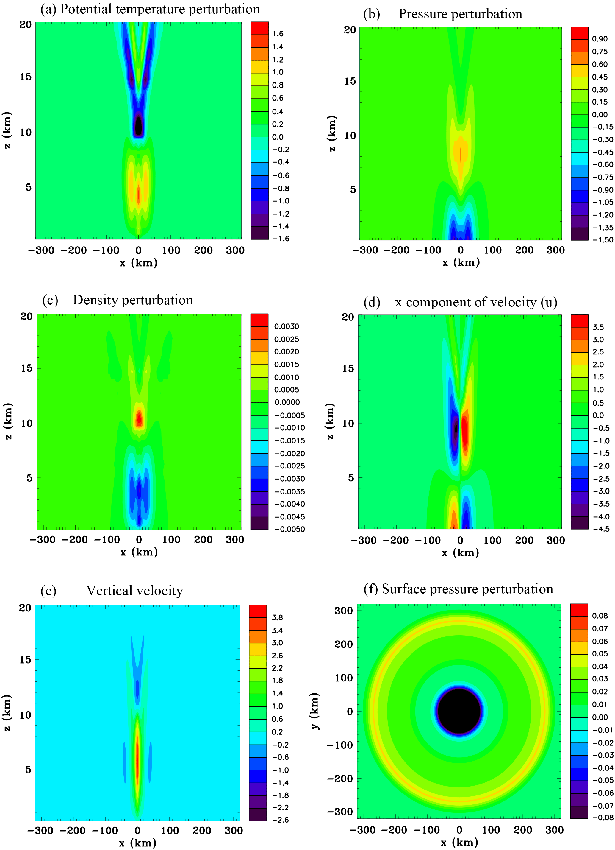
Figure 7Vertical sections for the convective-scale heat source, Experiment 1A, at t=15 mins. (a) Potential temperature perturbation (K), (b) pressure perturbation (hPa), (c) density perturbation (kg m−3), (d) x component of velocity (m s−1), (e) vertical velocity (m s−1), and (f) surface pressure perturbation (hPa).
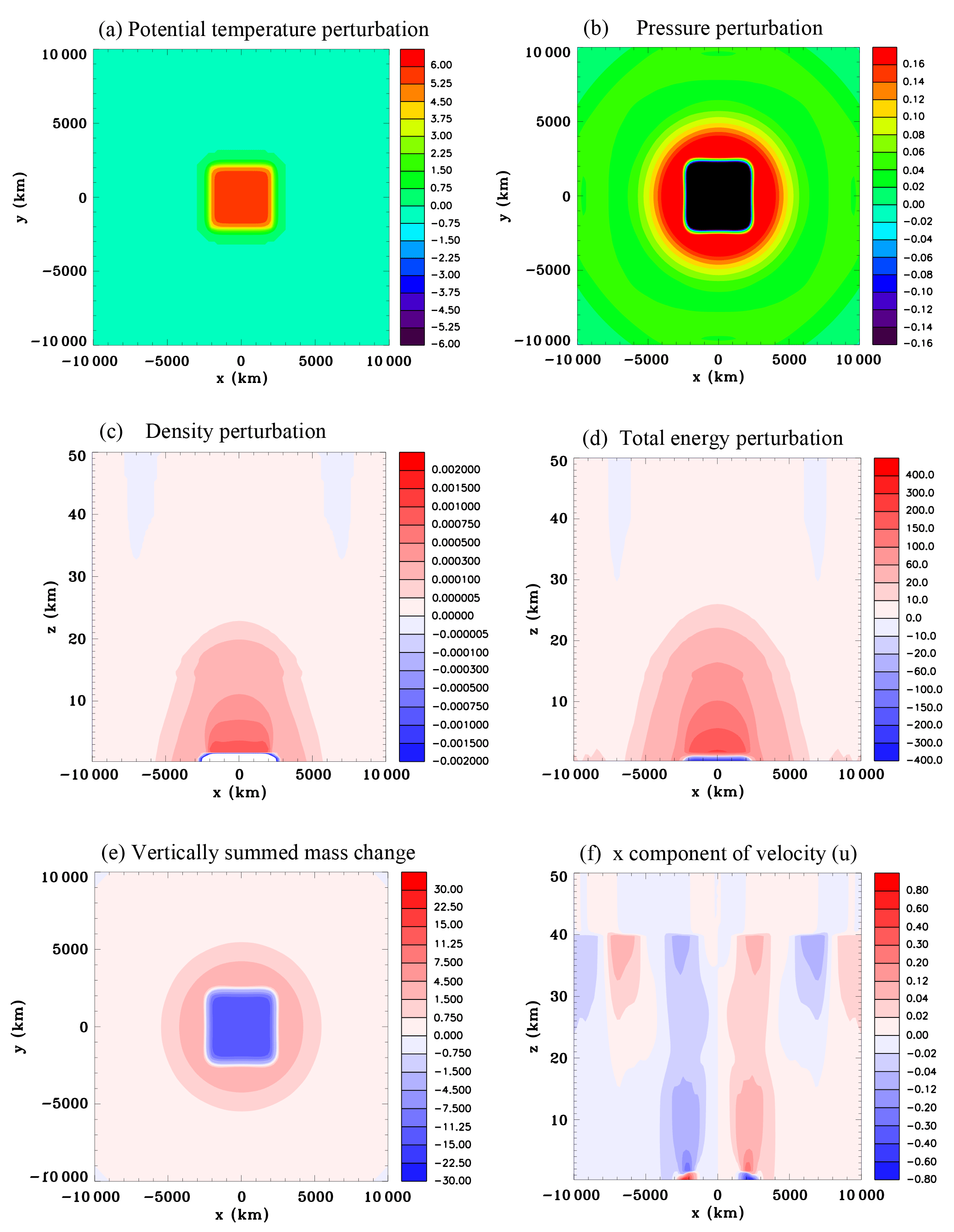
Figure 8Continent-scale heat source, Experiment 2A, at t=9 h. (a) Surface potential temperature perturbation (K), (b) surface pressure perturbation (hPa), (c) vertical section of the density perturbation (kg m−3), (d) vertical section of the total energy perturbation (J m−3), (e) vertical summed mass change (kg m−2), and (f) x component of velocity (m s−1).
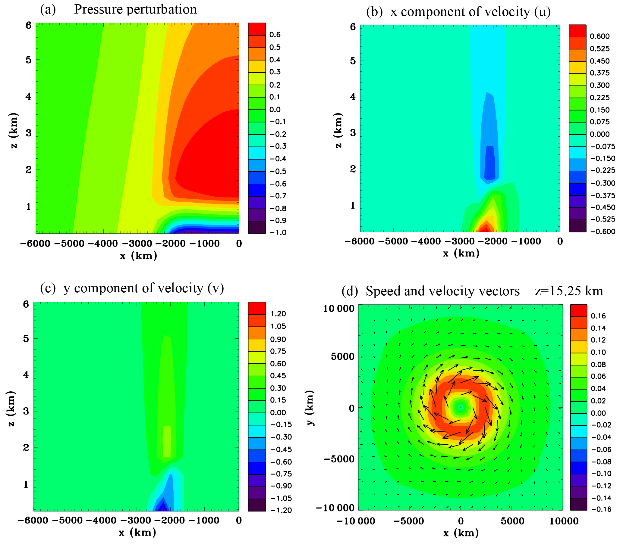
Figure 9Continent-scale heat source, Experiment 2A, at t=9 h. Zoomed-in vertical sections through the center of the domain of (a) pressure perturbation (hPa), (b) x component of velocity (m s−1), (c) y component of velocity (m s−1), and (d) enlarged horizontal section of speed (m s−1) and wind vectors at z=15.25 km.
NP94b showed a low-level horizontally homogeneous heat source results in compression of the air aloft throughout a deep layer. Associated with the mean upward motion in the troposphere and lower stratosphere are a mass flux and an energy flux. From Eq. (1) the rate of change of total energy to a good approximation for a dry atmosphere is given by the convergence of the energy flux:
where w is the vertical velocity. The simulation by NP94b showed the pressure perturbation rapidly increasing with height to the top of the thin heated layer adjacent to the surface and then falling off exponentially above (Fig. 7 of that paper). Also the density decreased significantly in the heated layer and increased very slightly above but throughout a much deeper layer. These positive pressure and density perturbations aloft represent significant increases in internal and gravitational potential energy throughout a deep region above the low-level heat source, and a net convergence of the energy flux given by Eq. (4) must have occurred at each level.
Later on in the simulation a turbulent boundary layer developed. The turbulent sensible heat flux was calculated and shown at low levels to a very good approximation equal to the upward total energy flux. This is an expected result since after all this is the way the enthalpy flux from the surface is in practice calculated. However, prior to the turbulent boundary layer thermals developing there was still an upward enthalpy flux. This flux did not depend on the presence of thermals, but only on the vertical expansion of the low-level air.
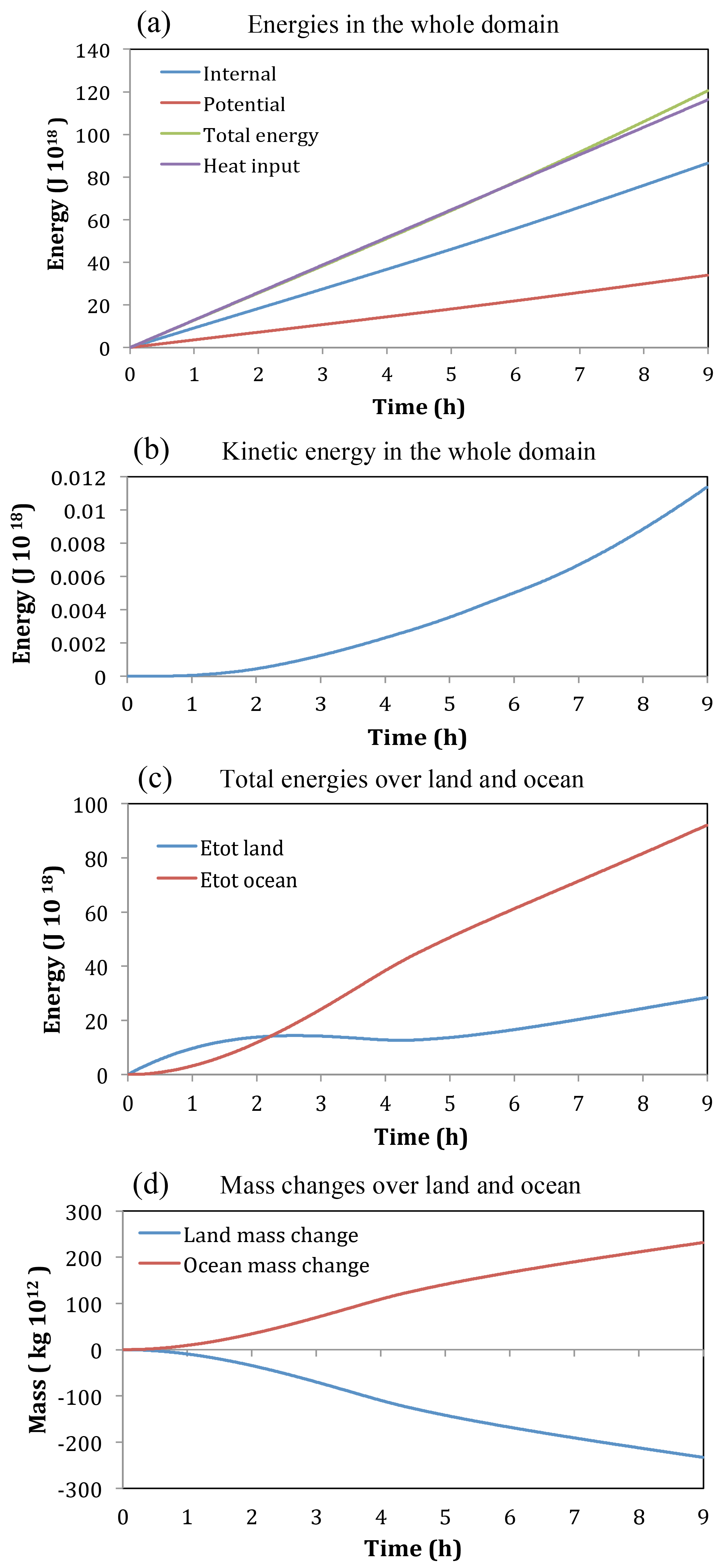
Figure 10Time series for the continent-scale heat source, Experiment 2A. (a) Internal energy, potential energy, total energy, and heat input; (b) kinetic energy; (c) energies over land and ocean (J ×1018); and (d) mass changes over land and ocean (kg ×1012).
As part of this current modeling study we have conducted a simulation with a model top at 140 km with a 20 km deep Rayleigh friction layer. The results remain similar to NP94b, showing a significant increase in the total energy up to the lower stratosphere in response to a low-level heat source. Therefore if one wanted to calculate the net heat input, and also calculate the increase in the perturbation energy field in response to this net heat input, then the calculation would have to integrate vertically through a large depth, into the stratosphere, to get a reasonable agreement between them.
2.6 Lamb waves
Solutions to the linearized equations for a stratified fluid show the existence of three types of waves known as acoustic waves, Lamb waves, and gravity waves (e.g., Gill, 1982). The restoring force for acoustic and Lamb waves is compression, and for gravity waves it is buoyancy. The properties of Lamb waves have been discussed by numerous researchers (e.g., Lamb, 1910, 1932; Taylor, 1936; Lindzen and Blake, 1972). A feature of this wave is that for an isothermal atmosphere its velocity is parallel to the surface, so the vertical velocity is zero.
The vertical structure of Lamb waves for an isothermal atmosphere is given by
where is the scale height with T0 the basic state temperature and . Since γ−1 is greater than zero, it can be seen that the perturbation horizontal velocity u′ increases with height, whereas the perturbation pressure p′ and density ρ′ decrease with height. NP94b modeled a two-dimensional sea-breeze circulation produced by a surface heat source that was turned off after an hour. The solution at 2 h showed Lamb waves had moved offshore on either side of the land surface.
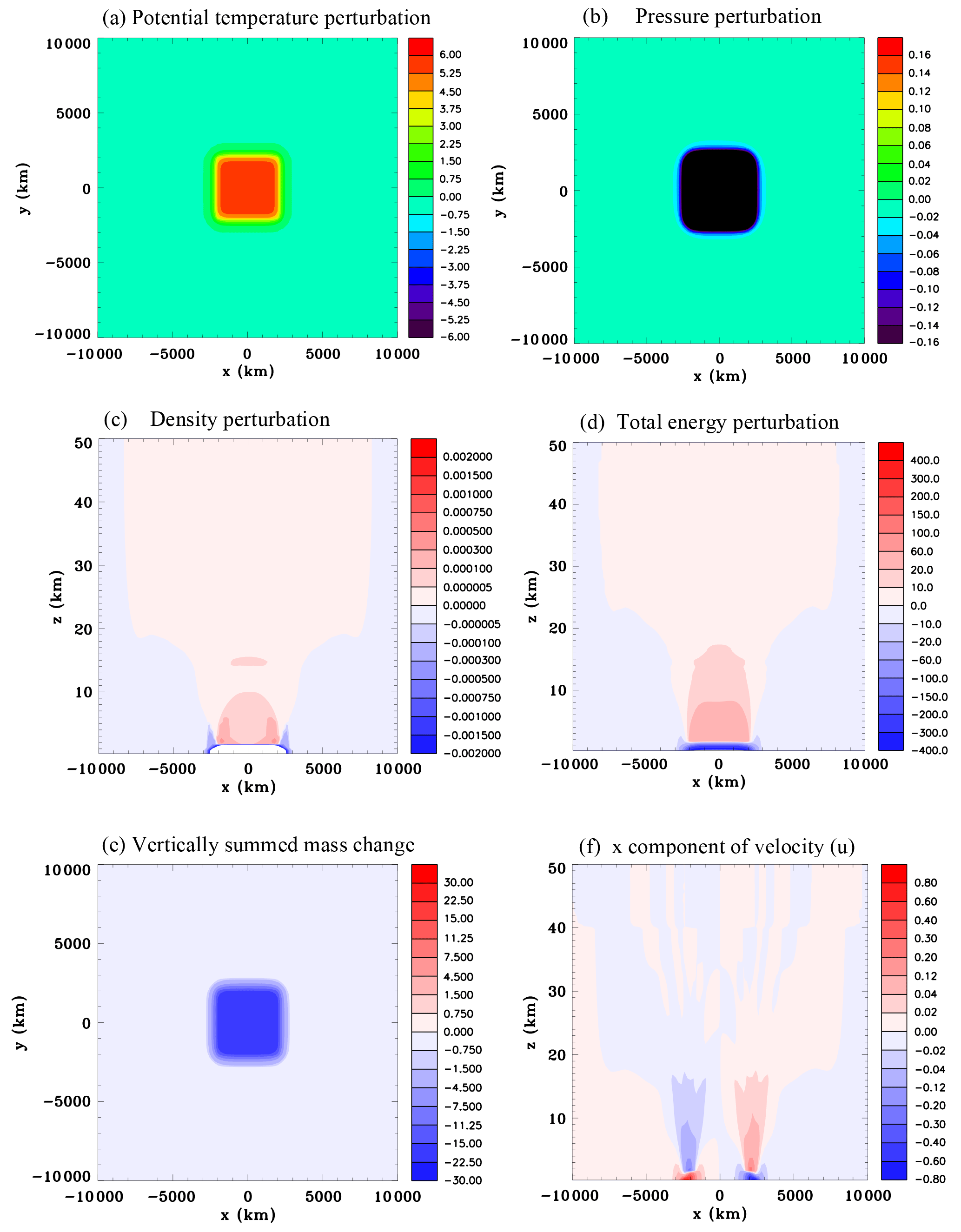
Figure 11Continent-scale heat source without compression waves, Experiment 2B, at t=9 h. (a) Surface potential temperature perturbation (K), (b) surface pressure perturbation (hPa), (c) vertical section of the density perturbation (kg m−3), (d) vertical section of the total energy perturbation (J m−3), (e) vertically summed mass change (kg m−2), and (f) x component of velocity (m s−1).
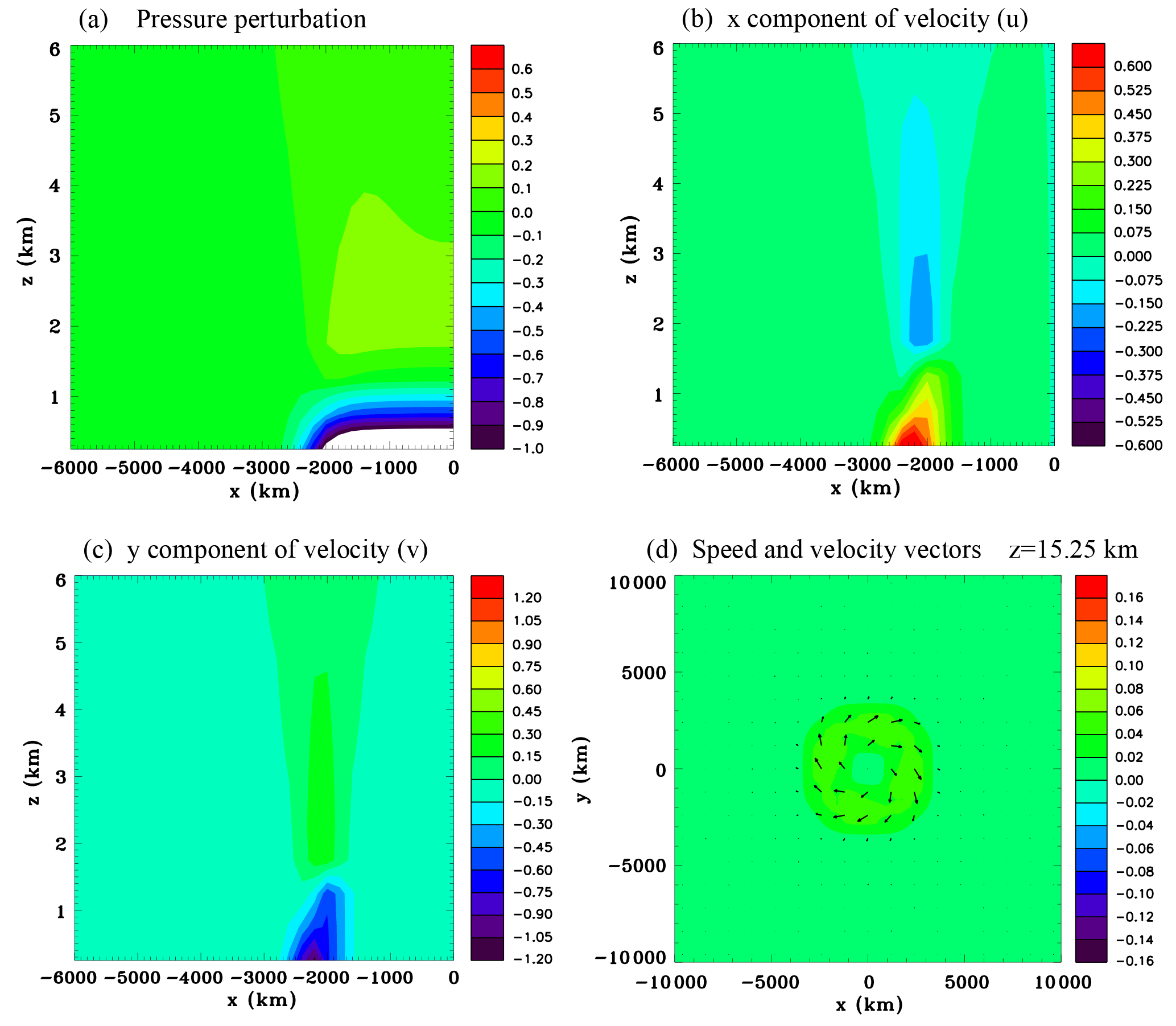
Figure 12Continent-scale heat source without compression waves, Experiment 2B, at t=9 h. Zoomed-in vertical sections through the center of the domain of (a) pressure perturbation (hPa), (b) x component of velocity (m s−1), (c) y component of velocity (m s−1), and (d) enlarged horizontal section of speed (m s−1) and wind vectors at z=15.25 km.
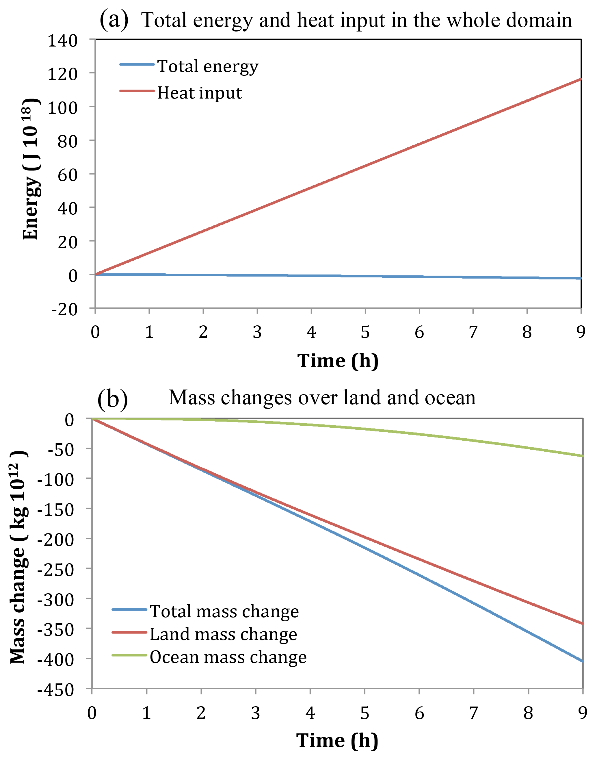
Figure 13Time series for the continent-scale heat source without compression waves, Experiment 2B. (a) Total energy and heat input (J ×1018), and (b) mass changes over land and ocean (kg ×1012).
Nicholls and Pielke (2000) using a fully compressible version of the Regional Atmospheric Modeling System (RAMS) modified to include sources and sinks of water vapor simulated an isolated convective storm. They found a Lamb wave emerged from the storm, which was trailed by slower-moving gravity wave modes. An analysis of internal and gravitational potential energies showed that the net total energy within the Lamb wave, propagating away at the speed of sound, was approximately equal to the net latent heat release that had taken place in the convective storm. It was noted that because the Lamb wave propagated in the horizontal plane it had a two-dimensional character. For instance, whereas a heat source in one dimension creates a compression wave with only a positive pressure perturbation as in Fig. S2, in two dimensions a leading positive pressure anomaly is trailed by a negative pressure anomaly (Fig. 2 of Nicholls and Pielke, 2000). This geometric effect on the shape of sound waves is well known (e.g., Lighthill, 1978).
These results suggest that thermally generated Lamb waves are likely to be ubiquitous in the atmosphere and moreover that they play a significant role in horizontal transfers of total energy and mass. Unlike for acoustic waves there is no cutoff frequency, so very low-frequency Lamb waves can be produced by convective forcing. Nishida et al. (2014) studied background Lamb waves in the Earth's atmosphere. They found evidence of Lamb waves with frequencies from 0.2 to 10 mHz based on array analysis of microbarometer data with a root mean square (rms) amplitude of about 0.15 Pa. In their assessment of excitation mechanisms they emphasized turbulence as the probable source for the background Lamb waves. However, it is possible that thermally generated Lamb waves caused by latent heat release in storms could have contributed based on the results of Nicholls and Pielke (2000).
2.7 To what extent can these thermally generated disturbances be considered waves?
While we use the term thermal compression waves to refer to large regions of compressed air moving at the speed of sound that are generated by heat sources, it is important to recognize that they do not satisfy every criterion usually associated with waves. For instance, waves are often considered a periodic disturbance of the particles of a substance and after their passage there is no resultant movement of the particles. Sometimes a wave is defined as a process that transports energy without transporting mass. In contrast, the pressure pulse in Fig. S2 is not periodic and its passage leads to a net movement of the fluid particles. There is clearly a mass transfer in this process.
While it might be considered stretching the definition of a wave to refer to these thermally generated disturbances as waves, there is little doubt that a thermally generated disturbance like the one that propagated at the speed of sound in the simulation of a convective storm by Nicholls and Pielke (2000) would be regarded as a wave-like feature if it was detected by a microbarometer array.
2.8 Thermally generated gravity waves
In the numerical experiments discussed later in this paper the prescribed heat sources also generate gravity waves as well as compression waves, so in order to get a better understanding of these simulations a brief review is given in this section. Bretherton and Smolarkiewicz (1988) drew attention to the link between gravity waves and compensating subsidence in the environment surrounding a convective cloud. The spreading gravity wave response to a developing cloud was investigated using a two-dimensional simulation. They found that a buoyancy source caused vertical displacements in the air in a widening region around the cloud which for this two-dimensional framework made the buoyancy of the environment approximately equal to the buoyancy in the cloud.
Nicholls et al. (1991) derived simple analytical two-dimensional solutions to the linear hydrostatic Boussinesq equations for an atmosphere at rest with prescribed heat sources and sinks. For a case with an idealized rigid lid and a deep heat source, represented by a half-sine wave in the vertical, the thermally generated buoyancy circulation was characterized by upward motion in the heated region with outflow aloft and inflow at low levels. The outflow and inflow expanded rapidly on either side of the heat source. The leading edges of these expanding circulations were deep fast-moving wave-like pulses of subsidence. Therefore, the subsidence compensating the central upward motion did not occur continually over broad regions on either side of the heat source, but had a distinct horizontally propagating character. The propagating subsidence regions caused adiabatic warming, adjusting the environmental potential temperature towards the perturbed values at the heated center for this two-dimensional framework. Response to a thermal-forcing profile more typical of a mesoscale convective system (MCS) having a stratiform region was also examined for a rigid lid. In this case a deep rapidly propagating circulation like the one previously discussed was superimposed on a slower-propagating circulation characterized by a mid-level inflow and upper- and lower-level outflows. This second slower-moving mode had a cool potential temperature anomaly at low levels and a warm potential temperature anomaly aloft. The leading pulses of vertical motion had upward motion at low levels and downward motion aloft. The speed of the modes is given by
where N is the Brunt–Väisälä frequency; H the height of the rigid lid; and n the wave number of the vertical heating with a vertical structure sin(nπz∕H), where z is height.
The two-dimensional solution for a semi-infinite region, without a troposphere–stratosphere interface, shows considerable differences of the low-level fields in some respects (Pandya et al., 1993). In particular, the magnitude of the subsidence is substantially reduced and occurs over a much broader region. Moreover, the axis of the peak vertical velocity in the low-level subsidence region is no longer vertically aligned, but strongly tilted. Nevertheless, adiabatic warming behind the broader wavefront still gradually approaches the values at the heated center. Another factor to consider is that in the real atmosphere there is increased stability above the tropopause, which partially reflects waves and to some extent increases the similarity with the rigid lid solution. A two-dimensional squall line simulation by Nicholls (1987) showed a structure similar to the analytic solution for the first mode during the early stage of development. The deep convective heating extending to the top of the troposphere produced a deep overturning circulation with surface mesolows growing laterally away from the center of the convection at a rapid pace. For the first deep convective mode that extends throughout the depth of the tropical troposphere, H is approximately 15 km and taking N=0.01 s−1 gives a horizontal propagation speed of 48 m s−1. For the second mode, the speed is 24 m s−1. These speeds are much faster than typical atmospheric motions.
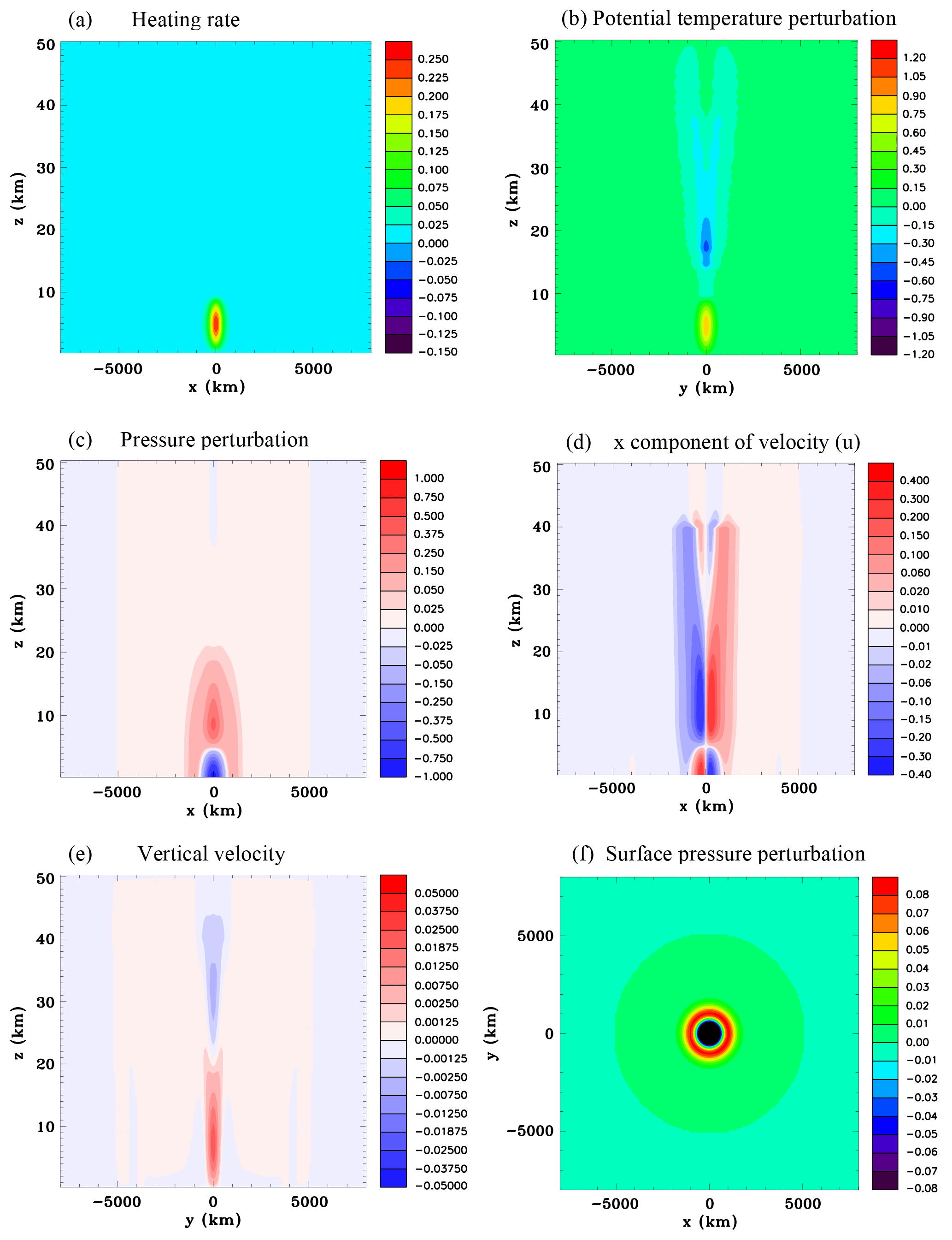
Figure 14Equator heat source, Experiment 3A, at t=1 h. (a) x∕z section of the heating rate (J kg−1 s−1), (b) y∕z section of the potential temperature perturbation (K), (c) x∕z section of the pressure perturbation (hPa), (d) x∕z section of the x component of velocity (m s−1), (e) y∕z section of the vertical velocity (m s−1), and (f) surface pressure perturbation (hPa).
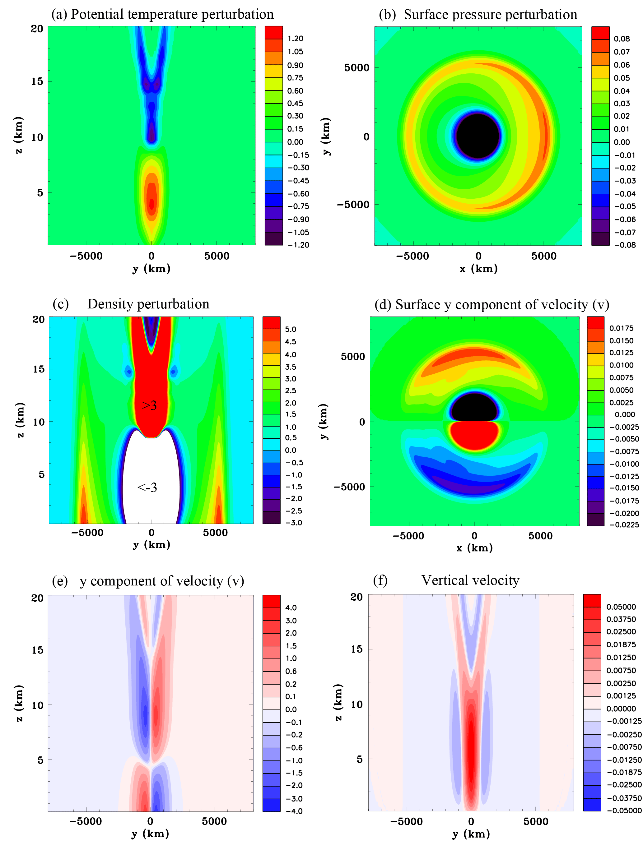
Figure 15Equator heat source, Experiment 3A, at t=5 h. (a) Potential temperature perturbation (K), (b) surface pressure perturbation (hPa), (c) density perturbation (kg m, (d) y component of velocity at the surface (m s−1), (e) y component of velocity (m s−1), and (f) vertical velocity (m s−1). Note that the vertical sections are all y∕z sections (meridional).
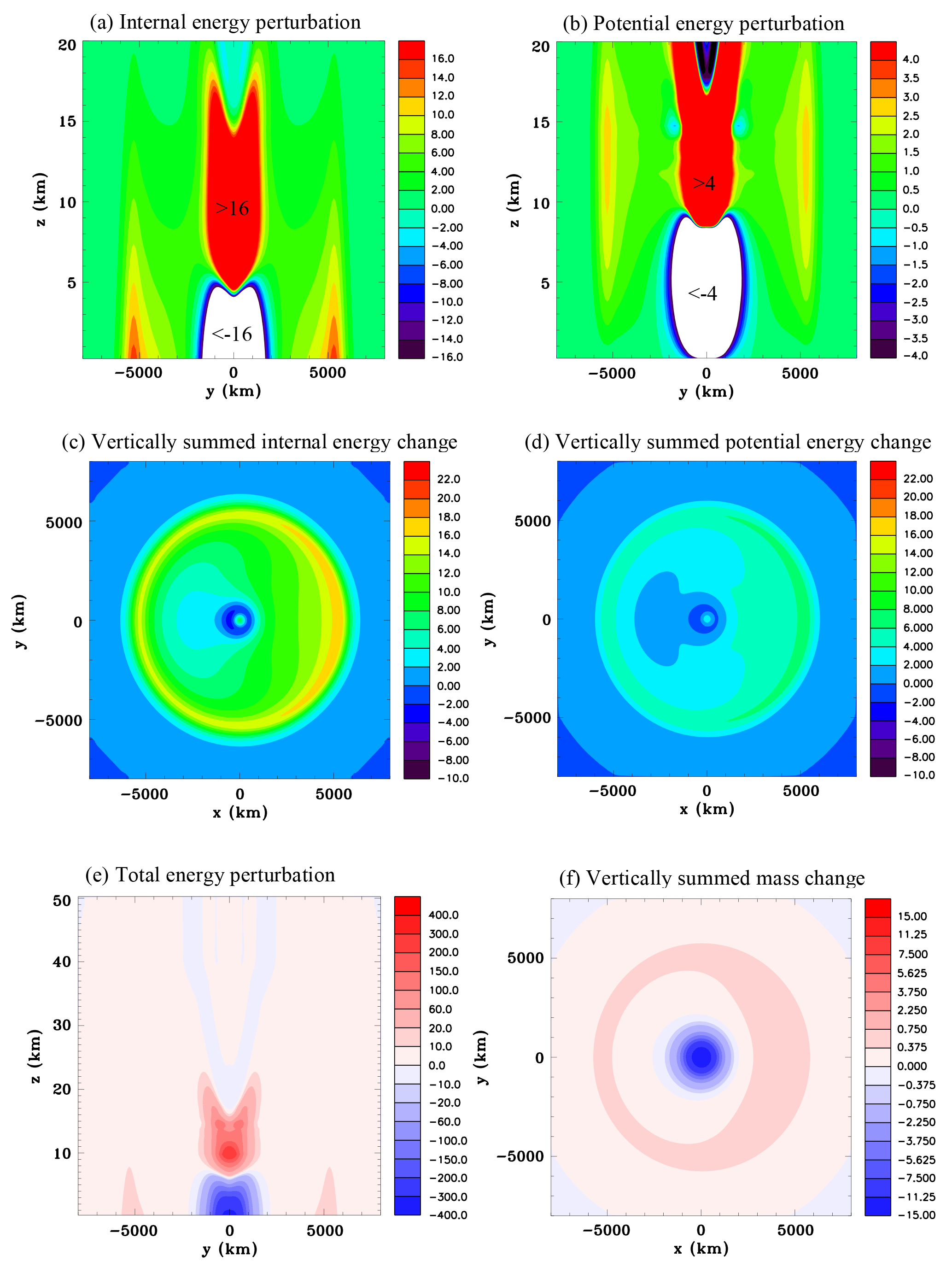
Figure 16Equator heat source, Experiment 3A, at t=5 h. (a) Internal energy perturbation (J m−3), (b) potential energy perturbation (J m−3), (c) vertically summed internal energy perturbation (J m, (d) vertically summed potential energy perturbation (J m, (e) total energy perturbation (J m−3), and (f) vertically summed mass change (kg m−2).
Mapes (1993) postulated that higher-order modes of the heating profile in a MCS may cause upward displacements at low levels in the nearby atmosphere, thus favoring the development of additional convection nearby. He also emphasized that the wave-like disturbances are not ordinary gravity waves, and pointing out their similarity to tidal bores in water, referred to them as buoyancy bores. There has been a considerable amount of research since these earlier studies that has examined their role in convective systems (e.g., Pandya et al., 2000; Nicholls and Pielke, 2000; Haertel and Johnson, 2001; Fovell et al., 2006; Tulich and Mapes, 2008; Bryan and Parker, 2010; Adams-Selin and Johnson, 2013). Inclusion of planetary rotation confines the compensating subsidence and adiabatic warming caused by deep convection to a finite distance, measured by the Rossby radius of deformation (e.g., Liu and Moncrieff, 2004).
The studies by NP94a and b were motivated by the finding that thermally generated gravity waves simulated with the standard version of RAMS (without the terms on the right side of Eq. 10 discussed in the next section) were not transferring significant amounts of total energy and moreover that there was a considerable discrepancy between the heat input and the net total energy increase within the domain. This led to the conclusion that thermally generated compression waves, which were eliminated from the RAMS model equations, might be the explanation for the missing energy.
RAMS is a nonhydrostatic numerical modeling system comprising time-dependent equations for velocity, non-dimensional pressure perturbation, ice-liquid water potential temperature (Tripoli and Cotton, 1981), total water mixing ratio, and cloud microphysics (Pielke et al., 1992; Cotton et al., 2003). In this study simulations are conducted without moisture. The model uses a time-splitting procedure which provides numerical efficiency by treating the sound wave modes separately (Derickson, 1974; Klemp and Wilhemson, 1978). To obtain the most accuracy for these simulations very small time steps were used and the time-splitting scheme was not employed. The model uses a similar approach to Klemp and Wilhelmson (1978) and utilizes the Exner function given by
The Exner function is a scaled measure of pressure with the reference pressure p00=1000 hPa. It is decomposed into a time-independent reference state Π0, which is a function of height and that is determined from the initial input pressure profile, and a perturbation Π′. The prognostic equation for Π′ is written in tensor form as
where uj () are the velocities u, v, w, respectively; and θv is the virtual potential temperature. The variables c0, ρ0, and θ0, are reference state values of the speed of sound, density, and potential temperature, respectively. Klemp and Wilhelmson (1978) note that the terms on the right side of this equation appear to have little influence on processes which are of physical interest in the cloud model. Their model was coded so that these terms could be included or omitted. They found that omission of these terms can allow small amounts of mass to be added or removed from the domain, which in turn affects the mean level of the pressure. Furthermore they liken this behavior to that occurring in the anelastic system where non-uniqueness of the Poisson solution requires an arbitrary specification of the mean pressure. Typically simulations with RAMS do not include the terms on the right side of Eq. (10); however, Medvigy et al. (2005) used the full equation for a study that examined mass conservation. For previous studies of thermal compression waves we have used the density instead of the Exner function, which was prognosed from the continuity equation (NP94a and b), and a different form of Eq. (10) which includes a moisture source or sink (Nicholls and Pielke, 2000). For this study we use Eq. (10). The advantage of using this form of the equation is that inclusion or not of the third term, with the material derivative of virtual potential temperature, acts as a switch for allowing or not allowing thermally generated compression waves. Therefore the effects of thermally generated compression waves can be more readily evaluated.
Preliminary experiments that examined large-scale transfer of total energy showed distortions of the compression waves occurring at large distances from the source. In order to improve accuracy the model code was modified for double precision.
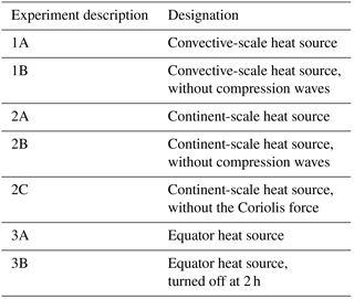
There are three main experiments conducted for this study and several auxiliary experiments. The first shows the response to a deep convective-scale heat source. The fields are portrayed in detail, showing the air expanding in the heated region creating a compression wave in the surrounding air and shortly after the development of a buoyancy-driven circulation. An auxiliary experiment examines the effect of not including the first three terms on the right side of Eq. (10), which eliminates compression waves. The second main experiment has a continent-scale heat source prescribed near the surface in a square region and includes a constant value of the Coriolis parameter specified for a latitude of 45∘. The purpose is to show that there is a considerable transport of total energy and mass to large distances offshore. An auxiliary experiment examines the effect of not including compression waves. Another auxiliary experiment examines the effect of turning off the Coriolis force. The third main experiment has a heat source located at the equator which is the size of a large cloud cluster and includes a Coriolis force that varies with latitude. The purpose of this experiment is to examine the resultant meridional transfer of total energy and mass. An auxiliary experiment examines the effect of turning the heat source off after a short period so that the compression wave can separate from the more slowly propagating buoyancy-driven circulation. Table 1 lists the experiments.
The model is configured with 101 vertical levels and a vertical grid increment of 500 m. Below the model top which is at 50 km there is a 10 km Rayleigh friction layer in order to damp upward-propagating waves, thereby reducing reflection. There are 161 horizontal grid points both in the x direction and y direction for all experiments. For the first experiment the horizontal grid increment is 4 km, giving a domain width of 640 km. The heating function is
where Q0 is the magnitude of the heat source, H=10 km, and a=12 km. The simulation is run for a 15 min period. For the continent-scale heat source simulation the horizontal grid increment is 200 km, giving a domain width of 32 000 km. The heat source is horizontally homogeneous for a square region in the center of the domain with sides of length 4000 km. In the vertical the heat source is a quarter cosine between the surface and 1 km. In effect this means the heating source is applied at the first thermodynamic grid point above the surface, which is at 250 m, and at the second thermodynamic grid point above the surface, which is at 750 m. The simulation is run for a period of 9 h. For the third experiment the horizontal grid increment is 100 km, giving a domain width of 16 000 km. The heating function has the same form as Eq. (11) except a=500 km. The simulation is run for a period of 5 h. For Experiment 3B the heating is turned off after 2 h.
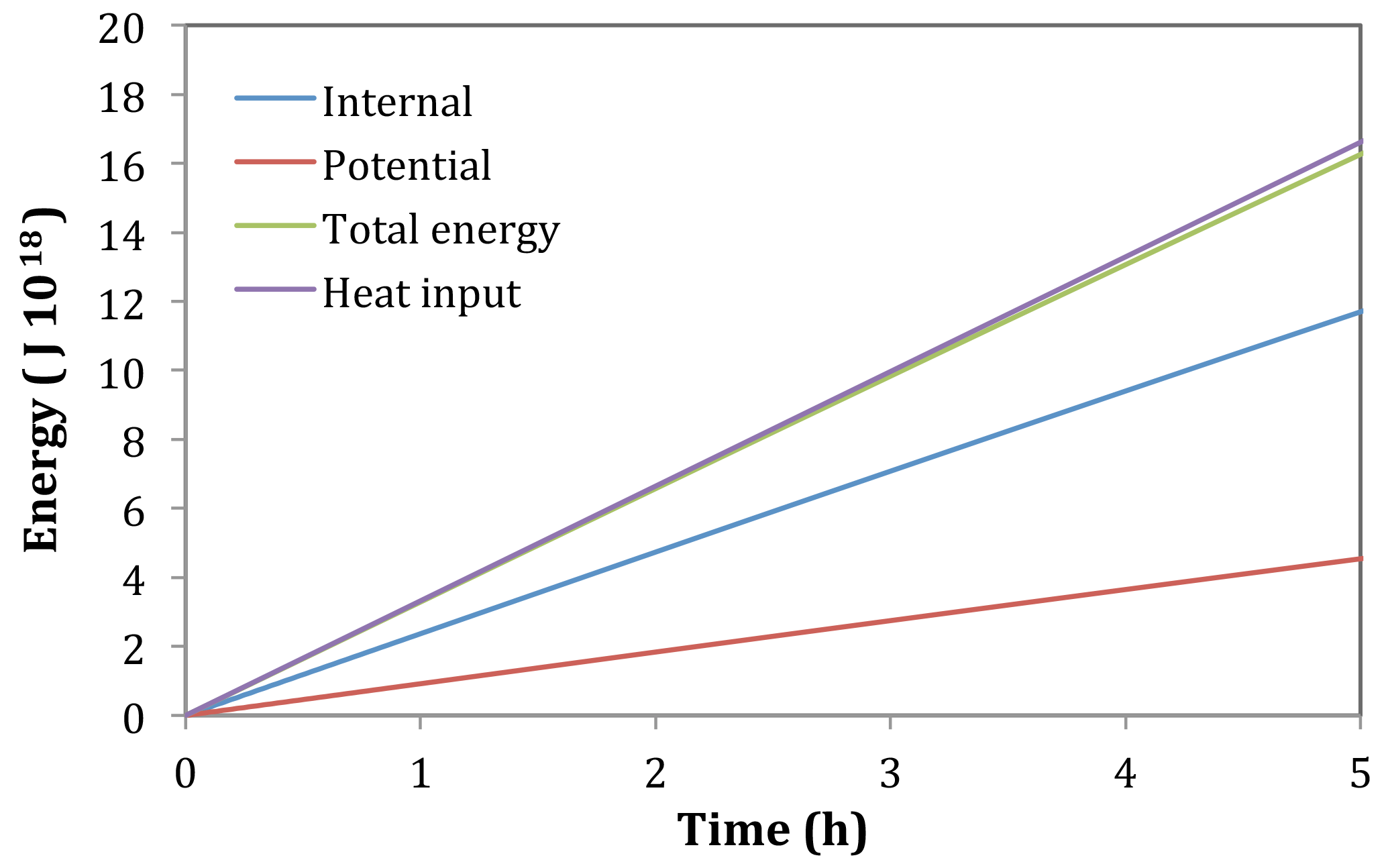
Figure 17Time series for the equator heat source, Experiment 3A. Internal energy, potential energy, total energy, and heat input (J ×1018).
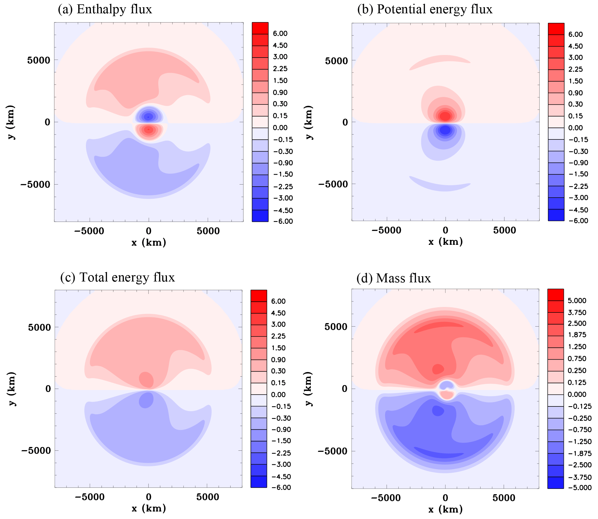
Figure 18Vertically summed meridional fluxes for the equator heat source, Experiment 3A, at t=5 h. (a) Enthalpy flux (W m, (b) potential energy flux (W m, (c) total energy flux (W m, and (d) mass flux (kg s−1 m.
The initial temperature profile is the mean Atlantic hurricane season sounding of Jordan (1958) up to 50 hPa, and above this level the US Standard Atmosphere profile was used (e.g., Wallace and Hobbs, 1977). The simulations were dry.
5.1 Convective-scale heat source
Figure 1 shows x∕z vertical sections through the center of the domain of the heating rate, temperature perturbation, pressure perturbation, x component of velocity u, and vertical velocity w, at 10 s. The heating causes the temperature and pressure to increase as would be expected and the pressure gradient is already starting to drive an outflow as can be seen in the velocity fields. Note that the pressure is starting to increase at the surface as the downward-propagating wavefront starts to reflect off it.
Figure 2 shows vertical sections of the density perturbation and the pressure perturbation at 20 s. The density, which is not a predicted variable, is diagnosed using the equation of state. The red–blue color scheme in this figure has a nonlinear scale in order to portray very small and very large values on the same figure. It can be seen that the density has started to decrease significantly in the core of the heated region as the air expands, while in the immediate surroundings of the heated region the air is compressed. The pressure field now shows a maximum at the surface. The higher pressure can be seen to be extending beyond the heat source.
Figure 3 shows vertical sections of the density perturbation, pressure perturbation, and vertical velocity at 40 s. The buoyancy created by the decreased density is starting to produce a significant updraft in the troposphere. Above this the updraft extends to a height of about 18 km. For a speed of sound of 320 m s−1 the distance a wavefront would travel in 40 s is around 12 km. Since the heating peak is at 5 km the compression wavefront reaching a height of ∼18 km is reasonable. At this time the surface pressure directly beneath the heat source has started to become negative due to lateral expansion causing the vertical column of air above the surface to weigh less.
Figure 4 shows vertical sections of u at 80 s and w at 120 s. At 80 s there is now an inflow at low levels and an outflow in the upper troposphere associated with the buoyancy-driven circulation. At 120 s in addition to the strong updraft in the mid-troposphere there is subsidence beginning to develop in the immediate surroundings, which is again a feature of the buoyancy-driven circulation.
Figure 5 shows vertical sections of w at 60 and 90 s, which extend to the top of the domain at 50 km in order to portray the vertical propagation of the compression wave. The wavefront quickly propagates upwards at the speed of sound. It can be seen that the magnitude of vertical velocity in the upward-propagating wave increases at it travels upwards. A second maximum is evident at 90 s, which is due to reflection of the downward-propagating wavefront seen at Fig. 1e at the surface.
Figure 6 shows vertical sections of the density perturbation and horizontal sections of the surface pressure perturbation at 5 and 10 min. Note that the color bar intervals are chosen to illustrate the very small perturbations in the compression wave. At 5 min the positive density perturbation at the leading edge of the compression wave has reached 100 km from the center of the heat source. The density perturbation decreases with height approximately as would be expected for a Lamb wave (Eq. 7). There is a ring of high pressure at the surface. By 10 min the compression wave has propagated to approximately 200 km from the storm. Interestingly the high-pressure anomaly is concentrated in a narrow ring at the leading edge and so has a different shape than for the 1-D thermal compression wave solution, shown in Fig. S1 in the Supplement. This is likely to be mainly a geometric effect since thermally generated Lamb waves have a two-dimensional character when propagating in three dimensions away from a localized heat source as discussed in Sect. 2.6.
The features of the buoyancy-driven simulation are illustrated in Fig. 7, which shows fields at 15 min. Even for this simple constant heat source the response is quite complicated. The warm region at the center of the heat source is surrounded by an annulus of warm air. There is a v-shaped region of cool air aloft. A low-pressure anomaly occurs at the surface and a high-pressure anomaly at the top of the heat source. The density perturbation is similar in shape to the potential temperature perturbation although of opposite sign. As expected there is a strong inflow at low levels and outflow at the top of the heat source. Upward motion is in the center and compensating subsidence in the surrounding air. There is a wave-like character to the buoyancy circulation, such that the ring of subsidence is propagating away from the heat source with a speed of approximately 45 m s−1. This subsidence results in adiabatic warming. This propagating character and structure has similarities to the highly idealized solutions discussed in Nicholls et al. (1991) for the deep rapidly propagating convective mode. Figure 7e shows that by 15 min the leading edge of the compression wave has almost propagated to 300 km and is considerably lower in amplitude than at 10 min (Fig. 6d).
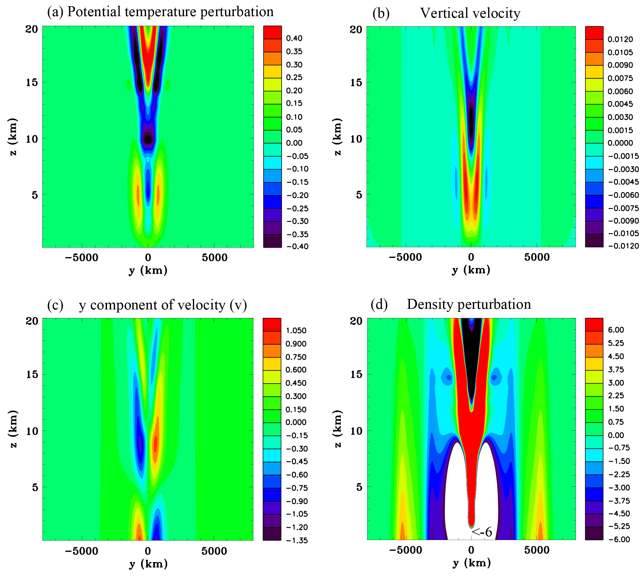
Figure 19Equator heat source with a duration of 2 h, Experiment 3B, at t=5 h. (a) Potential temperature perturbation (K), (b) vertical velocity (m s−1), (c) y component of velocity (m s−1), and (d) density perturbation (kg m.
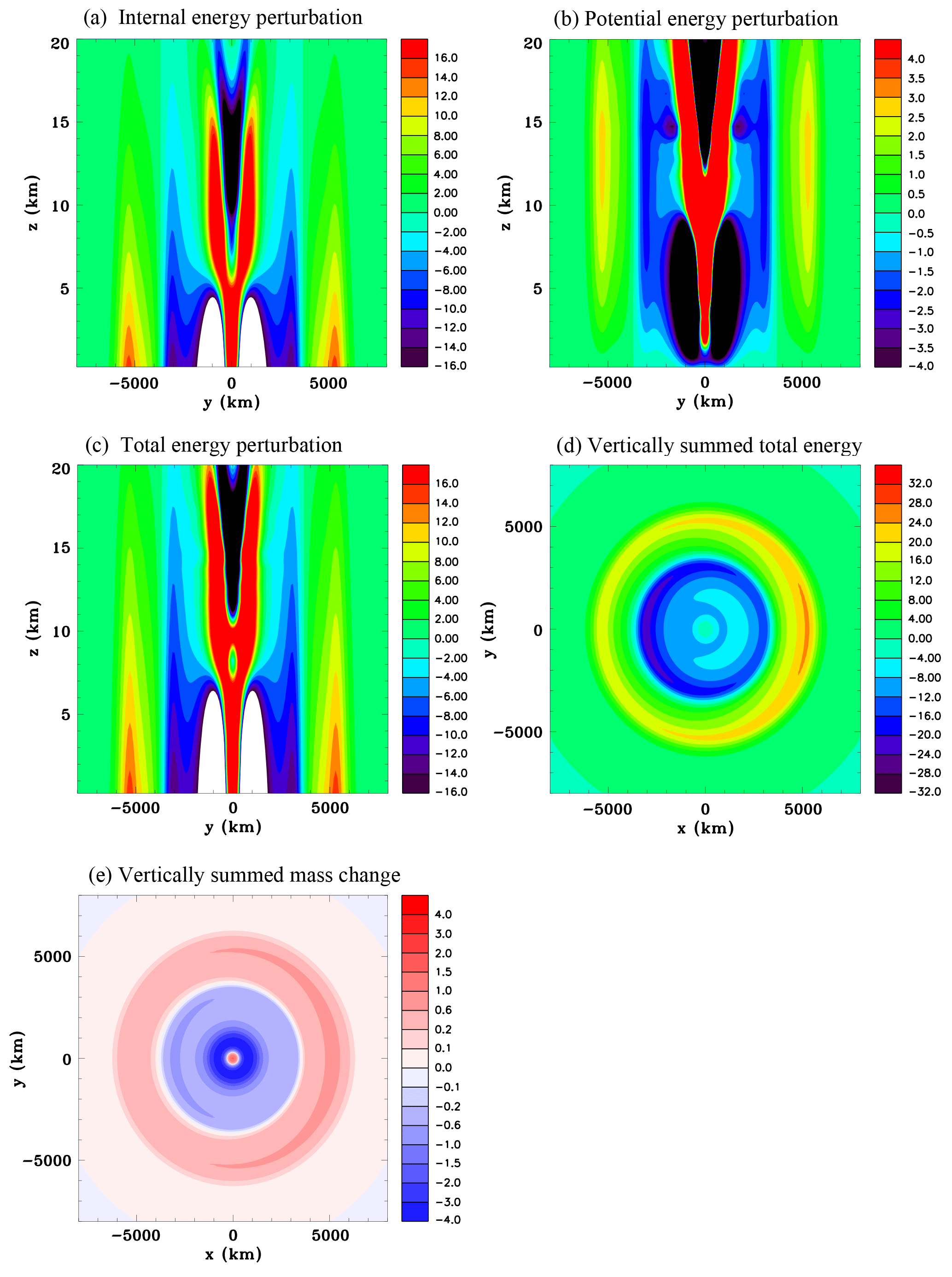
Figure 20Equator heat source with a duration of 2 h, Experiment 3B, at t=5 h. (a) Internal energy perturbation (J m−3), (b) potential energy perturbation (J m−3), (c) total energy perturbation (J m−3), (d) vertically summed total energy perturbation (J m, and (e) vertically summed mass perturbation (kg m−2).
Results for the convective-scale heat source with the terms on the right side of Eq. (10) omitted (Experiment 1B) are shown in the Supplement (Sect. S3 and Figs. S5–S7). Early in the simulation (Fig. S5) there are significant differences with the fully compressible solution (Fig. 1). In particular, there is no expansion of the air evident in the horizontal and vertical velocity fields. Instead of showing expansion, the circulation has an inflow at low levels and outflow at the upper region of the heat source with a deep updraft at the center. Moreover the surface pressure immediately starts to decrease at the surface and there is no increase in the surrounding environment. Despite significant differences with the fully compressible case early on in the simulation, by 15 min the results are virtually identical (compare Figs. S7 and 7).
These results corroborate the conclusion by Klemp and Wilhelmson (1978) that the terms on the right side of Eq. (10) are not important for cloud modeling, at least if one is not interested in the very low-amplitude compression waves that are generated. However, it shall be seen for the continent-scale heat source that differences are more pronounced. Also as Klemp and Wilhemson (1978) noted, for convective cloud simulations there can be a small amount of mass change within the domain, which is evident from Fig. S7b since the mean surface pressure has been reduced (assuming that the pressure field does not deviate that much from hydrostatic). As will be discussed in Sect. 6, mass changes could be more significant if diabatic heat sources are large or if they occur throughout the whole domain, which can be the situation if radiation is included.
5.2 Continent-scale heat source
In this section the response to horizontally homogeneous heating at the surface of a square continent is considered. Figure 8 shows results at 9 h for Experiment 2A, which has the Coriolis force included. The surface potential temperature over the heated land surface has increased by approximately 6 K. The surface pressure has decreased considerably over the land and has increased by ∼0.16 hPa over the adjacent ocean (note a small color bar interval has been chosen for Fig. 8b to illustrate the relatively small pressure increase over the ocean, which means that the magnitude of the surface pressure drop over land is not discernible). A vertical section through the center of the continent of the density perturbation (Fig. 8c) shows a large decrease near the surface (note that due to the small color bar interval the large decrease over land is not colored) and a smaller amplitude increase above and over the adjacent ocean. The total energy perturbation consisting of internal, gravitational potential, and kinetic energy has increased in a large dome-shaped region except for a decrease in a thin layer next to the land surface (Fig. 8d). It can be seen that the total energy has increased significantly into the lower stratosphere, but not at higher levels, which is consistent with the discussion of Sect. 2.5. Figure 8e shows the field of vertically integrated total mass change (this can be considered the change in a square meter oblong column extending from the surface to the top of the domain). The mass has decreased over the land area and has increased over the surrounding ocean area. Figure 8f shows a vertical section of the zonal velocity u. At the west and east edges of the land surface there are low-level inflows and just above are return flows. These are very crudely resolved sea breezes. There is a deep layer of weak offshore flow aloft. While some of this offshore flow is associated with the return flow of the sea breeze, a part of this flow is due to expansion of the air occurring above the continent. Below the Rayleigh friction layer there is a wave-like structure aloft. These are propagating at the speed of sound and the leading edge of the first anomalies have passed beyond the west and east sides of the panel at −10 000 and 10 000 km, respectively (note that the model domain size is much larger than the panel size shown in this figure). This wave-like appearance of the velocity field aloft is primarily a geometrical effect as discussed in Sect. 2.6 and is not nearly so evident in a two-dimensional simulation (not shown). It has ramifications for the fluxes of energy and mass off the continent as will be discussed shortly.
Figure 9 zooms in on the west side of the domain to show details of the sea-breeze circulation. There is a dome of positive pressure anomaly over a surface negative pressure anomaly. The total energy perturbation field in Fig. 8d mainly reflects these pressure perturbations. The y component of velocity v is negative near the surface because the Coriolis force turns the inflow winds to the right, whereas the opposite occurs in the overlying sea-breeze return flow. Figure 9d shows a horizontal section of a larger portion of the domain at z=15.25 km illustrating an outflow aloft above the shoreline and a weak anticyclonic flow of several centimeters per second above the ocean that looks like it might be close to a gradient wind balance since it encircles the dome of high pressure.
Figure 10 shows time series of the summed energies throughout the whole domain and the heat input. The gravitational potential energy at any time is almost exactly two-fifths of the internal energy as would be expected for a hydrostatically balanced circulation where they would differ by a factor of R∕cv. The total energy in the domain is the same as the heat input until 7 h, after which it becomes slightly larger. It is not clear why this small discrepancy occurs. The kinetic energy is shown on a different panel because it is so much smaller in magnitude than the internal and potential energies.
The summed energies shown separately for the land and ocean in Fig. 10c show an interesting behavior. The total energy initially increases quickly over land. As shown in Fig. 3 of NP94b the pressure initially increases in the heated layer adjacent to the surface, but there is an offshore mass flux as the air expands, causing the surface pressure to begin to fall a short distance inland. This outflow associated with expansion of air works its way inland at the speed of sound. It takes a little under 2 h for this outflow to reach the center of the domain, which for this simulation is 2000 km from the shoreline. Upward fluxes of mass and energy occur above the whole of the land surface as soon as the simulation begins (for example Fig. 13 of NP94b illustrates an upward sensible energy flux, or enthalpy flux, caused by a horizontally homogeneous low-level heat source). Since in the early stage of the simulation there is only an upward component to the energy flux over most of the land surface, and the lateral offshore flux at the coastline is small, then the net total energy over land initially increases quickly. However, offshore lateral fluxes of energy at the shoreline, while small to begin with, increase quite rapidly, such that after 2 h the total energy over land no longer increases despite the heat input and actually starts to decline. This increase in the offshore flux appears to be because all the air across the whole continent is undergoing lateral expansion by 2 h, whereas initially it was only air near the coast. Figure 8f shows a wave train in the zonal velocity field (u) at upper levels. The regions in the wave train, with a flow towards the land, started to develop over the continent at 3 h, and by 5 h there was a significant onshore flow above 25 km. This coincided with the total energy over the land increasing again. By 9 h there is again a deep region of offshore flow at the shoreline (Fig. 8f), but not as strong as at 2 h, and the total energy over land is continuing to increase.
The time series of the mass changes over land and ocean shown in Fig. 10d are mirror images of one another. This indicates there is reasonably good mass conservation. The rate of mass change is slow to begin with, strongest between 2 and 5 h, and then changes at a moderate rate. This behavior would be expected from the evolution of the normal component of velocity (u) at the shoreline discussed in the previous paragraph.
Figure 11 shows results at 9 h for Experiment 2B without thermal compression waves and can be compared with Fig. 8. The surface potential temperature change is identical. There is a pressure decrease over land, but there is no increase over the surrounding ocean. The density decreases where heating occurs, but does not show much increase aloft or any significant increase over the ocean, unlike Experiment 2A. The vertical section of the total energy perturbation does not show a pronounced dome. There is a net mass decrease over the land, but no matching increase over the ocean, so that mass is not being conserved. While a sea breeze is evident there is not a deep offshore flow at the shoreline.
Figure 12 zooms in on the west side of the domain for Experiment 2B similarly to Fig. 9. The pressure drop over the land is considerably larger for this simulation compared to the fully compressible result. For the compressible case there is a larger density increase aloft comparing Fig. 8c with Fig. 11c, so that the weight of a column of air above the surface is greater, which is why the pressure fall is not so much. For this simulation the inflow is larger, whereas the return flow aloft is smaller when compared to the compressible simulation. This can be explained by the expansion of air over the continent for the compressible simulation contributing an offshore component to the flow (Fig. 8f), which at low levels can be thought of as superimposed on the buoyancy-driven sea-breeze circulation. Since the onshore flow is larger for this simulation the Coriolis force causes the meridional component of the wind to be larger in magnitude as well. These differences of the wind speeds are approximately 15 %, so while not large they are significant. Figure 12d shows the flow aloft above the shoreline is only about one third of the strength as occurred for the fully compressible simulation (Fig. 9d). Moreover there is no anticyclonic flow at a large distance offshore.
Time series for the total energy in the domain and mass changes over the land and ocean for Experiment 2B are shown in Fig. 13. The total energy in the whole domain decreases slightly with time even though there is a large heat input showing there is no energy conservation. The mass in the domain decreases linearly with time and this is mainly over the land mass. The sea-breeze circulation tends to bring some mass onshore, which results in a decrease over the ocean.
Results for Experiment 2C, which is fully compressible but does not include the Coriolis term, are shown in the Supplement (Sect. S4 and Figs. S8 and S9). Comparing with Experiment 2A there is far more total energy and mass redistributed over the ocean and to greater distances offshore. For sea-breeze circulations the horizontal extent is comparable to the Rossby radius of deformation, which can be considered approximately the buoyancy frequency N times a height scale for the convective boundary layer divided by the Coriolis parameter, with modifications due to surface friction (e.g., Rotunno, 1983; Dalu et al., 1991; Drobinski and Dubos, 2009). Without the Coriolis force the horizontal extent of the sea breeze is considerably larger and is stronger in magnitude than for Experiment 2A at 9 h, as would be expected (not shown). The horizontal scale for geostrophic adjustment associated with the fast-propagating Lamb wave shown in Fig. 9d is clearly much larger than that of the sea breeze in Fig. 9c, since the anticyclonic flow is quite strong even at 2000–3000 km offshore. The length scale given by the speed of sound divided by the Coriolis parameter at 45∘ latitude is approximately 3000 km. For this f-plane simulation this length scale can be considered to be a Rossby radius of deformation for these very fast-moving compression waves (e.g., Gill, 1982).
5.3 Equator heat source
In this section the response to a heat source with the scale of a cloud cluster and which is located at the equator is examined (Experiment 3A). Figure 14 shows a vertical section through the center of the heat source and several panels of simulated fields at 1 h for Experiment 3A. There are quite a few similarities to the convective-scale heat source. A compression wave is generated which at this early stage is quite symmetrical, as can be seen by the surface pressure perturbation. Figure 15, with vertical sections that only go to a height of 20 km, shows that by 5 h a significant asymmetry has developed as the compression wave has traveled far enough away from the equator to become influenced by the Coriolis force. The potential temperature has increased by just over 1 K in the center of the heat source. The warm region has widened due to the compensating subsidence (Fig. 15f). The compression wavefront has reached about 6000 km from the source as can be seen in Fig. 15b, c, and d. It appears that as the wavefront reaches higher latitudes the Coriolis force acts to turn the weak outflow to the right in the Northern Hemisphere and to the left in the Southern Hemisphere, resulting in a convergence of mass to the east of the heat source and a divergence of mass to the west, and this results in an asymmetrical surface pressure field. For instance, Fig. 15d shows that the meridional component of the outflow is stronger to the west of the heat source than to the east. The height–meridional vertical section of the density field shown in Fig. 15c, which has a very small color bar interval to portray the compression wave, indicates mass redistribution towards the polar regions. Figures 15e and f indicate that the leading edge of the thermally generated buoyancy circulation is propagating at a speed of ∼45 m s−1 in the meridional direction.
Figure 16 focuses on the energy and mass changes at 5 h for Experiment 3A. The height–meridional section of the internal energy perturbation shows that the leading pulse of the compression wave is a region of enhanced internal energy. This field is identical to the perturbation pressure except for the multiplication factor of cv∕R. There are much larger positive and negative perturbations in the region of the buoyancy-driven circulation, but these tend to cancel each other out. The density perturbation at the leading edge of the compression wave, shown in Fig. 15c, results in positive gravitational potential energy perturbations that are maximized in the upper troposphere and lower stratosphere. The fields of vertically summed internal and gravitational potential energy perturbations show maxima to the east of the source, but clearly there has been a significant meridional transfer towards the polar regions (Fig. 16c and d). The changes at the center of the heat source are relatively small. Therefore the heat source has not caused a significant in situ increase in total energy when the vertical sum is considered. Figure 16e shows a height–meridional section of the total energy perturbation, which goes to the top of the domain. The largest anomaly in the compression wave occurs just over 5000 km from the heat source. The major anomalies occur in the region of the buoyancy-driven circulation, but vertically integrated they tend to cancel. Figure 16f shows the mass has decreased in the region of the buoyancy-driven circulation where there has been net lateral expansion of the air, whereas it has increased in the surrounding environment. The mass changes in the surrounding environment are much smaller in magnitude, but occur over a much larger area.
Time series of the energies and heat input for the whole domain are shown in Fig. 17. Again the potential energy can be seen to be two-fifths of the internal energy to a good approximation. For this simulation the total energy is slightly less than the heat input at the end of the 5 h simulation, demonstrating reasonable energy conservation.
Meridional fluxes that have been summed in the vertical are portrayed in Fig. 18. Shown are the vertical sums of the fluxes of enthalpy ρcpTv, gravitational potential energy ρgzv, total energy , and mass ρv. The procedure was to use values of the variables at the center of each grid volume to calculate the flux crossing the area ΔxΔz, where Δx is the width of the grid volume in the x direction and Δz is the height, and then these meridional fluxes for the grid volumes were summed vertically from the bottom to the top of the domain. Dividing by Δx gives the fluxes per unit meter. The enthalpy flux is quite strong at the leading edge of the compression wave and is towards the poles. Interestingly the flux is towards the equator in the region occupied by the buoyancy-driven circulation. The strong low-level flow towards the heat source (Fig. 15e) and the fact that pressure is higher at low levels compared to aloft are apparently the cause of this net equatorward flux (note that the enthalpy flux can also be written as using the ideal gas law, which makes clear the dependence on pressure). The potential energy flux on the other hand shows the opposite behavior in the region of the buoyancy-driven circulation. Since the potential energy is small at low levels, the strong outflow in the upper troposphere dominates the transport. The total energy flux illustrates that a significant meridional transport away from the equator is occurring between the heat source and the leading edge of the compression wave. Figure 18d demonstrates that there is also a broad region of meridional mass transport away from the equator, except for a small region very close to the heat source.
Results for Experiment 3B at 5 h, which is identical to Experiment 3A except the heat source is turned off after 2 h, are shown in Fig. 19. There is no longer a warm potential temperature perturbation at the center, but instead a warm air anomaly in a ring that surrounds a cool anomaly at the center. This warm ring is propagating as subsidence causes adiabatic warming at its leading edge and ascent causes adiabatic cooling at its trailing edge. In between the downdraft and updraft the winds are towards the center in the lower troposphere and away from the center in the upper troposphere. So there is an overturning circulation that propagates through the environment away from where the heat source was located in a wave-like manner, which has similarities to the idealized linear two-dimensional rigid lid solution for a pulse-forcing function discussed in Nicholls et al. (1991). This thermally generated gravity wave, or buoyancy bore (Mapes, 1993), propagates significantly slower than the thermally generated compression wave, so that by this time the two wave types are starting to become separated. The Lamb wave is evident in the density perturbation field shown in Fig. 19d and it can be seen that it has a leading lobe with a positive anomaly and a trailing lobe with a negative anomaly, which as mentioned previously in Sect. 2.6 is a geometric effect due to the Lamb wave having a two-dimensional character for a localized compact source in three dimensions. The idealized one-dimensional solution for a thermal compression wave shown in Fig. S2 of the Supplement on the other hand has a simpler structure and does not exhibit a leading positive lobe trailed by a negative lobe.
Energies and mass changes for Experiment 3B are shown in Fig. 20. The leading lobe of the Lamb wave has positive internal and potential perturbation energies, whereas as the trailing lobe has negative perturbation energies. Figure 20d shows the negative values of the vertically summed total energy perturbation in the trailing lobe are as large in amplitude as the positive values in the leading lobe, but they occupy a much smaller area so there is still a net positive total energy in the Lamb wave. Moreover by the time the negative lobe was to reach the same distance from the source as the positive lobe, it would have decreased significantly in amplitude. At the center the vertically summed total energy perturbation is slightly negative. Positive values of vertically summed total energy perturbation are only found at over 3000 km from the center of where the heat source was located. The vertically summed mass change has a large negative value in the area occupied by the thermally generated gravity wave, weak negative values in the trailing lobe of the compression wave, and weak positive values in the leading lobe. This indicates that a significant redistribution of mass has occurred at the speed of sound.
The current paradigm of large-scale meridional transport of internal and gravitational potential energies assumes it is accomplished in an advective-like manner with the winds. The results of this study suggest that significant transports could be occurring at the speed of sound. The simulations in this study are highly idealized, but it seems unlikely that this transport mechanism would not be occurring in the real atmosphere. To what degree is currently unknown. The decomposition of Eq. (3) has been the standard procedure for many years with an interpretation that attributes the meridional fluxes to advective-like transports by transient eddy, stationary eddy, and mean meridional circulations. This study has not considered energy transfer in the presence of eddies that transport warm air poleward and cold air equatorward. However, it could be imagined for the equator heat source experiment that there was a large-scale eddy at midlatitudes transporting warm air poleward and cold air equatorward and that a Lamb wave produced by a rapidly intensifying cloud cluster or tropical cyclone near the equator propagated polewards through it – for instance, in a similar manner as portrayed by Figs. 14f and 15b that shows the rapidly propagating surface pressure perturbation. This is analogous to the scenario discussed in Sect. 2.4. Presumably the fast-moving Lamb wave would not be too influenced by the much slower winds of the large-scale eddy.
Suppose for the sake of argument that the large-scale eddy was not producing meridional sensible and potential energy fluxes prior to the arrival of the Lamb wave. As the Lamb wave passed through the eddy there would be poleward meridional sensible and potential energy fluxes. The flux would be associated with very small increases in the meridional velocity, pressure, density, and temperature. If Eq. (1) was used, the enthalpy flux could be either calculated using the density and temperature or from the pressure after substitution from the ideal gas law (ignoring the effects of moisture for simplicity). It is perhaps worth mentioning that these perturbations associated with the passage of the Lamb wave are very small and would be extremely difficult to measure from atmospheric observations, although in a modeling study this would be feasible. Alternatively the right side of Eq. (2) could be used to calculate the energy transport. In this case the bounds of the integral vary since the surface pressure rises as the Lamb wave propagates through the eddy. So care should be taken when attributing the fluxes just to the terms in the integrand since the bounds of the integral are changing, which affects the value of the integral.
A fundamental aspect of the transfer of total energy as the Lamb wave propagated poleward through the large-scale eddy is that it would involve a mass transfer (e.g., Fig. 16f). This raises the possibility that there might be issues with the methodologies used to calculate the contributions to total energy transport in Eq. (3) because these very rapid mass transfers at the speed of sound are not properly accounted for. Both observational and modeling studies typically enforce mass constraints when calculating meridional energy transports (e.g., Masuda, 1988; Keith, 1995; Magnusdottir and Saravanan, 1999; Graversen et al., 2007; Yang et al., 2015; Liang et al., 2018). Perhaps this could be causing the attribution of energy transports to be misinterpreted. This issue would need to be examined in a modeling study that simulated more realistic atmospheric circulations than in this work. The equations used by RAMS use some approximations that are reasonable for cloud and mesoscale simulations and for the relatively small departure from the basic state in these simulations. However if this model was used to simulate large-scale baroclinic eddies, which would require significant meridional temperature gradients, then modifications to the model equations would probably need to be made to obtain accurate mass and energy conservation.
Many weather and climate models use the hydrostatic balance condition and the governing equations include Lamb waves as solutions. Therefore they may be capable of simulating some of the compressibility effects that have been investigated using fully compressible nonhydrostatic models including propagation of total energy at the speed of sound. However, the use of semi-implicit time differencing schemes, which has become common, brings this into question. Such schemes are considered of great practical utility since they slow down fast-moving modes thought to have little meteorological significance, thereby allowing the use of a much larger model time step (e.g., Robert, 1969, 1993; Tapp and White, 1976; Tanguay et al., 1990; Simmons and Temperton, 1997). Typically Lamb waves will be slowed down and distorted by these methods. However, thermally generated Lamb waves do have physically significant effects, so the use of semi-implicit schemes may be causing more inaccuracy than has been recognized in large-scale global models. For instance, if the thermally generated compression wave shown in Fig. S2 were slowed down while maintaining total energy and mass conservation then it would need to be larger in magnitude. Moreover geostrophic adjustment due to the Coriolis force acting on the horizontal velocities associated with Lamb waves would presumably occur over a smaller spatial scale.
Semi-implicit methods may also have an impact on thermally generated gravity waves. A study of orographic gravity waves was carried out by Shutts and Vosper (2011) using the Met Office Unified Model. They found that the semi-implicit off-centering parameter approach used by the model actually damped orographic waves in a global forecast if a large time step of 15 min was used. However, reducing the time step to 2 min allowed the orographic gravity waves to be adequately simulated. The results of this study raise the possibility that the large time steps typically used in global models may not only be significantly impacting thermally generated compression waves, but also thermally generated gravity waves. The physical importance of either of these thermally generated fast-propagating wave-like disturbances was not recognized at the time semi-implicit schemes were developed. They were designed for the purpose of eliminating the time step constraint imposed by fast-moving disturbances, such as mechanically produced sound waves, orographic gravity waves, and vertically propagating gravity waves above cloud tops, which were thought to be relatively unimportant for large-scale modeling.
Omission of the term responsible for generating thermal compression waves on the right side of Eq. (10) does not always lead to small mass changes in the model domain as Klemp and Wilhelmson (1978) suggested would be the case for a cloud simulation. For instance, hurricane simulations that include radiation and initially have no clouds will show an increasing mean surface pressure due to net radiative cooling, particularly at night when there is no shortwave warming counteracting longwave cooling, until enough latent heating occurs in the domain to counter this effect. Moreover inclusion of this term does not necessarily mean there will be no mass change in the domain. Fully compressible simulations with diabatic heating in clouds for instance will generate Lamb waves that propagate to the boundaries of the model domain, where if there are radiative boundary conditions they may end up being partially reflected. This is because while radiative boundary conditions are typically set up for the passage of slower-moving gravity waves they may not be perfectly reflective to faster-moving waves. So some mass may start to exit the domain. Such mass changes may not be a problem as far as the accurate simulation of typical meteorological processes are concerned, but it is something to be aware of.
The effects of thermally generated compression waves have yet to be fully assessed. It is likely that they are ubiquitous in the atmosphere, generated by diabatic heating caused by latent heat release, radiative forcing, and surface heating. Compression waves can also be caused by mass inputs and outputs due to water substance conversions such as evaporation from the surface. Since the amplitudes of these propagating disturbances are very small it might be assumed their effects are negligible, but in this study the case has been made that this is probably incorrect. Potentially the slowing down of thermally generated compression waves and gravity waves due to the use of semi-implicit schemes could be a source of error in climate models, but just how big these errors might be has yet to be evaluated.
Another issue that is brought up by the apparent role of Lamb waves in the transfer of total energy in the atmosphere is the meaning of the term “heat transfer”. It is common to think of heat as being carried from one place to another by the movement of relatively warm air, sometimes referred to as convective heat transfer. As was discussed in Sect. 2.4 this usage is different from how heat is typically defined in thermodynamics as energy in transit from one system to another by thermal interaction. Since the Earth's TOA radiative fluxes have a net input at low latitudes and output at high latitudes, then for an energy balance to occur in the mean there must be a poleward energy flux, given by the flux terms in Eqs. (1) and (2), and this has been termed a heat flux. This flux is complicated since it is comprised of fluxes of gravitational potential energy and latent heat, but it does at least have a term called the enthalpy flux, which is considered to be a convective heat flux that results in a transfer of internal energy. Now if a considerable amount of the internal energy is actually being transferred at the speed of sound and does not result in significant temperature perturbations as occurs in the numerical experiments in this study, then this further distances total energy transfer from what has been traditionally thought of to a large degree as a convective heat transfer. Certainly the transfer of total energy that occurs in these experiments with a fully compressible model would not correspond to what would normally be considered a transfer of heat.
Latent heat transport (water vapor) is a quantity that is advected with the wind so that the transfers associated with expansion and compression only apply to fluxes of dry enthalpy and gravitational potential energy. However, the current view is that, if energy is used to evaporate water at some location A and then the vapor is transported by air currents to another location B where it condenses, then energy has been transported from A to B. This is not such a simple thing to conclude, as it may seem, if the condensation produces a Lamb wave that quickly transports the energy hundreds of kilometers away at the speed of sound.
The first experimental setup in this study examined the response to a convective-scale heat source. The fully compressible version of the model showed in the early stages expansion of the heated air and compression of the adjacent environment. A few minutes after the heat source had been turned on, a laterally propagating Lamb wave emerged with the highest pressure and density anomalies at the surface with a wavefront that propagated away at the speed of sound. The reduction of density in the heated region produced buoyancy and a strong updraft developed with compensating subsidence in the nearby environment. This subsidence also propagated in a wave-like manner, but with a slower speed of ∼45 m s−1. The comparison with the standard version of RAMS that omits the term that involves the material rate of change of virtual potential temperature in Eq. (10) did not show expansion of air in the heated region or compression of the adjacent air. Nevertheless the diagnosed density still decreased in the heated region. A comparison at 15 min showed the thermally generated buoyancy circulation was virtually identical to that of the fully compressible simulation and so for most cloud modeling purposes the terms on the right side of Eq. (10) can be safely neglected as found by Klemp and Wilhelmson (1978).
So far there has been no study that can be said to have definitely observed the low-frequency Lamb waves generated by latent heat release in convective storms. Detection of thermally generated Lamb waves would bolster the conclusions from numerical modeling studies that they exist and could be playing a role in redistribution of total energy and mass. In this study the value of the positive surface pressure perturbation associated with the Lamb wave at a distance of 300 km from the heat source was approximately 0.05 Pa. The strength of the updraft was quite weak, only ∼4 m s−1, so this would only correspond to weak convection. For the NP2000 study, which simulated a strong convective storm and included liquid- and ice-phase microphysics, the magnitude of the pressure perturbations was considerably larger, having peak-to-peak values at 400 km from the storm of ∼0.6 Pa. The time interval between these positive and negative peaks was ∼20 min. Infrasound with periods of tens of seconds has been detected from severe weather (e.g., Bowman and Bedard, 1971); however, the only study to date that may possibly have detected low-frequency Lamb waves generated by latent heat release in convective storms was by Nishida et al. (2014), although they hypothesized the main excitation mechanism for the background Lamb waves to be atmospheric turbulence. As mentioned in Sect. 2.6 the rms amplitude of the Lamb waves they detected was 0.15 Pa, which falls within the range of these fully compressible simulations of convectively produced Lamb waves.
The second experimental setup examined the response to a continent-scale heat source applied near the surface. The surface pressure decreased over land and increased over the adjacent ocean. During the 9 h simulation there was significant lateral transfer of total energy and mass offshore as far as 3000 km from the shoreline. Approximately a third of the total energy increase occurred over land and two-thirds over the ocean. A similar simulation without compression waves showed a decrease in surface pressure over land, but no increase over the ocean. The net total energy did not increase in the domain even though there was a heat input and the net mass decreased. Comparing the horizontal velocities in the sea-breeze circulation, there was approximately a 15 % difference in their magnitudes. Running the fully compressible model without the Coriolis force resulted in much more total energy and mass transfer offshore, showing that geostrophic adjustment when the Coriolis force is included leads to significant confinement of the energy and mass. For this simulation, which has a constant Coriolis parameter, it is helpful to envisage a Rossby radius of deformation for Lamb waves (e.g., Gill, 1982), which is analogous to the Rossby radius of deformation for gravity waves where rotational effects become as important as buoyancy effects. This is given by the speed of sound divided by the Coriolis parameter, which for this experiment is approximately 3000 km. This Rossby radius is too large for the f-plane approximation to be valid (Gill, 1982), so while it is useful for understanding the results of this particular experiment it has limited utility when the Coriolis parameter more realistically varies with latitude.
The equator heat source experiment initially created a symmetrical response, but later on as the wavefront propagated to latitudes where the Coriolis force became important an interesting asymmetry developed. There was higher surface pressure to the east than the west and this was also reflected in the total energy and mass fields. The equator heat source produced significant meridional fluxes of enthalpy, potential energy, and mass. Turning the heat source off at 2 h allowed the thermally generated Lamb wave to start to separate from the slower-moving buoyancy circulation. The Lamb wave had a leading positive lobe of high pressure and a trailing negative lobe, which is a feature of a two-dimensional wave. Examining the vertically summed total energy perturbation field it was clear that the main region of increased energy in the domain in response to the heating was concentrated in the leading lobe of the Lamb wave several thousands of kilometers from the center of the heat source.
These findings reiterate previous results obtained many years ago that Lamb waves are able to transfer significant amounts of total energy at the speed of sound. It would be fair to say these earlier studies have had little impact on interpretations of the large-scale total energy transport. This current study, which shows the vertically summed energy fields, should reinforce the hypothesis that Lamb waves could indeed play a role in the large-scale transfer of total energy. There have been numerous observational and numerical modeling studies that calculate the meridional atmospheric fluxes of total energy and find a good agreement with the net global energy inputs and outputs (e.g., Masuda, 1988; Magnusdottir and Saravanan, 1999; Trenberth and Stepaniak, 2003; Yang et al., 2015). Therefore on the face of it there does not appear to be any problem with the current interpretation of atmospheric energy fluxes or the ability of state-of-the-art climate models to accurately simulate them. On the one hand we would contend that the results of this current study and previous works are unlikely to be fundamentally flawed, and this raises several questions. Are the studies showing considerable transfer of energy by Lamb waves too idealized and this transfer would be limited in a more realistic modeling framework? Do Lamb waves contribute significantly to the energy transport and global models are able to accurately simulate this transport, while perhaps there is a misinterpretation of the physical attribution to some degree? Is the slowing down of Lamb waves due to semi-implicit time differencing not really a substantial problem since it might be causing for the most part just a delayed response? On the other hand is the slowing down of Lamb waves not causing just a delayed response, but also significantly changing the spatial scale of the response as suggested in Sect. 6? Is the slowing down of Lamb waves due to semi-implicit time differencing causing them to have larger amplitude?
Another issue brought up by this study is that it has repercussions for the concept of heat transfer in a fluid. Total energy transfer is typically referred to as heat transfer, yet the mechanism of total energy transfer examined in this work does not have much connection to the more common notion of convective heat transfer. Finally, significant transfers of mass occurred at the speed of sound in these numerical experiments. If expansion and compression of air in response to heat sources and sinks leads to large lateral redistributions of mass at the speed of sound this may have consequences for understanding the mass balance that exists in the long-term mean in the atmosphere and perhaps seasonal variations.
The source code and model data (RAMS) used in this study are hosted by the Cooperative Institute for Research in Environmental Sciences (CIRES) at the University of Colorado, Boulder, United States. The data repository was created by the corresponding author and is located at http://cires1.colorado.edu/nicholls/data2/ (Nicholls, 2018) with the following identifier: http://cires1.colorado.edu/nicholls/data2/NP2018_data.tar.gz (last access: 11 October 2018).
The supplement related to this article is available online at: https://doi.org/10.5194/acp-18-15975-2018-supplement.
MEN and RAP Sr. designed the research and prepared the manuscript. MN conducted model simulations and data analysis.
The authors declare that they have no conflict of interest.
This research was primarily supported by Joan M. Nicholls. Support in part
was provided by the National Science Foundation, under grant NSF AGS
1445875. We are extremely grateful to Saurabh Barve for providing
computational assistance and appreciate the helpful suggestions from
Robert Walko, Stephen Saleeby, and Stephen Herbener for modifying the RAMS
code to enable double precision. We also thank two anonymous reviewers for
their constructive comments and suggestions.
Edited by: Heini Wernli
Reviewed by: two anonymous referees
Adams-Selin, R. D. and Johnson, R. H.: Examination of gravity waves associated with the 13 March 2003 bow echo, Mon. Weather Rev., 141, 3735–3756, 2013.
Beer, T.: Atmospheric waves, 300 pp., John Wiley, New York, 1974.
Bowman, H. S. and Bedard Jr., A. J.: Observations of infrasound and subsonic disturbances related to severe weather, Geophys. J. Roy. Astron. Soc., 26, 215–242, 1971.
Bretherton, C. S. and Smolarkiewicz, P. K.: Gravity waves, compensating subsidence and detrainment around cumulus clouds, J. Atmos. Sci., 46, 740–759, 1989.
Bryan, G. H. and Parker, M. D.: Observations of a squall line and its near environment using high-frequency rawinsonde launches during VORTEX2, Mon. Weather Rev., 138, 4076–4097, 2010.
Cotton, W. R., Pielke Sr., R. A., Walko, R. L., Liston, G. E., Tremback, C. T., Jiang, H., McAnelly, R. L., Harrington, J. Y., and Nicholls, M. E.: RAMS 2001: Current status and future directions, Meteor. Atmos. Phys., 82, 5–29, 2003.
Dalu, G. A., Pielke, R. A., Avissar, R., Kallos, G., Baldi, M., and Guerrini, A.: Linear impact of thermal inhomogeneities on mesoscale atmospheric flow with zero synoptic wind, Ann. Geophysicae, 9, 641–647, 1991.
Derickson, R. G.: Three dimensional modeling of orographic cloud systems, Preprints, Conferenec on Cloud Physics, Tucson, Arizona, 21–24 October, Amer. Meteor. Soc., 1974.
Drobinski, P. and Dubos, T.: Linear breeze scaling: from large-scale land/sea breezes to mesoscale inland breezes, Q. J. Roy. Meteorol. Soc., 135, 1766–1775, 2009.
Fovell, R. G., Mullendore, G. L., and Kim, S.-H.: Discrete propagation in numerically simulated nocturnal squall lines, Mon. Weather Rev., 134, 3735–3752, 2006.
Gill, A. E.: Atmosphere-ocean dynamics, International Geophysics Series, 30, Academic Press, New York, 1982.
Graversen, R. G., Kallen, E., Tjernstrom, M., and Kornich, H.: Atmospheric mass-transport inconsistencies in the ERA-40 Reanalysis, Q. J. Roy. Meteorol. Soc., 133, 673–680, 2007.
Haertel, P. T. and Johnson, R. H.: The linear dynamics of squall line mesohighs and wake lows, J. Atmos. Sci., 57, 93–107, 2000.
Jordan, C. L.: Mean soundings for the West Indies are, J. Meteor., 15, 91–97, 1958.
Keith, D. W.: Meridional energy transport: uncertainty in zonal means, Tellus A, 47, 30–44, 1995.
Klemp, J. B. and Wilhelmson, R. B.: The simulation of three-dimensional convective storm dynamics, J. Atmos. Sci., 35, 1070–1086, 1978.
Lamb, H.: On atmospheric oscillations, P. R. Soc. London, 84, 551–572, 1910.
Lamb, H.: Hydrodynamics, 6th edn., Cambridge University Press, London and New York, 1932.
Liang, M., Czaja, A., Graversen, R., and Tailleux, R.: Poleward energy transport: is the standard definition relevant at all time scales?, Clim. Dynam., 50, 1785–1797, 2018.
Lighthill, J.: Waves in fluids, Cambridge University Press, London and New York, 1978.
Lindzen, R. S. and Blake, D.: Lamb waves in the presence of realistic distributions of temperature and dissipation, J. Geophys. Res., 77, 2166–2176, 1972.
Liu, C. and Moncrieff, M. W.: Effects of convectively generated gravity waves and rotation on the organization of convection, J. Atmos. Sci., 61, 2218–2227, 2004.
Magnusdottir, G. and Saravanan, R.: The response of atmospheric heat transport to zonally-averaged SST trends, Tellus, 51, 815–832, 1999.
Mapes, B. E.: Gregarious tropical convection, J. Atmos. Sci., 50, 2026–2037, 1993.
Masuda, K.: Meridional heat transport by the atmosphere and the ocean: Analysis of FGGE data, Tellus A, 40, 285–302, 1988.
Medvigy, D., Moorcroft, P. R., Avisar, R., and Walko, R. L.: Mass conservation and atmospheric dynamics in the Regional Atmospheric Modeling System (RAMS), Environ. Fluid Mech., 5, 109–134, 2005.
Nicholls, M. E.: A comparison of the results of a two-dimensional numerical simulation of a tropical squall line with observations, Mon. Weather Rev., 115, 3055–3077, 1987.
Nicholls, M. E.: NP2018_data.tar.gz, available at: http://cires1.colorado.edu/nicholls/data2/, last access 11 October 2018.
Nicholls, M. E. and Pielke, R. A.: Thermal compression waves, I: Total energy transfer, Q. J. Roy. Meteorol. Soc., 120, 305–332, 1994a.
Nicholls, M. E. and Pielke, R. A.: Thermal compression waves, II: Mass adjustment and vertical transfer of total energy Transfer, Q. J. Roy. Meteorol. Soc., 120, 333–359, 1994b.
Nicholls, M. E. and Pielke Sr., R. A.: Thermally-induced compression waves and gravity waves generated by convective storms, J. Atmos. Sci., 57, 3251–3271, 2000.
Nicholls, M. E., Pielke, R. A., and Cotton, W. R.: Thermally forced gravity waves in an atmosphere at rest, J. Atmos. Sci., 48, 1869–1884, 1991.
Nishida, K., Kobayashi, N., and Fukao, Y.: Background Lamb waves in the Earth's atmosphere, Geophys. J. Int., 196, 312–316, 2014.
Oort, A. H. and Peixóto, J. P.: Global angular momentum and energy balance requirements from observations, Adv. Geophys., 25, 355–490, 1983.
Pandya, R., Durran, D., and Bretherton, C.: Comments on “Thermally forced gravity waves in an atmosphere at rest”, J. Atmos. Sci., 50, 4097–4101, 1993.
Pandya, R. E., Durran, D. R., and Weisman, M. L.: The influence of convective thermal forcing on the mesoscale circulaton around three-dimensional squall lines, J. Atmos. Sci., 57, 29–45, 2000.
Peixóto, J. P. and Oort, A. H.: Physics of Climate, American Institute of Physics, New York, 520 pp., 1992.
Pielke Sr., R. A., Cotton, W. R., Walko, R. L., Tremback, C. J., Lyons, W. A., Grasso, L. D., Nicholls, M. E., Moran, M. D., Wesley, D. A., Lee, T. J., and Copeland, J. H.: A comprehensive meteorological modeling system – RAMS, Meteorol. Atmos. Phys., 49, 69–91, 1992.
Priestley, C. H. B.: Heat transport and zonal stress between latitudes, Q. J. Roy. Meteorol. Soc., 75, 28–40, 1949.
Robert, A. J.: The integration of a spectral model of the atmosphere by the implicit method, WMO-IUGG Symposium on NWP, Tokyo, Japan Meteorological Agency, VII, 19–24, 1969.
Robert, A. J.: Bubble convection experiments with a semi-implicit formulation of the Euler equations, J. Atmos. Sci., 50, 1865–1873, 1993.
Rotunno, R.: On the linear theory of the land and sea breeze, J. Atmos. Sci., 40, 1999–2009, 1983.
Shutts, G. J. and Vosper, S. B.: Stratospheric gravity waves revealed in NWP model forecasts, Q. J. Roy. Meteorol. Soc., 137, 303–317, 2011.
Simmons, A. J. and Temperton, C.: Stability of a two-time-level semi-implicit integration scheme for gravity wave motion, Mon. Weather Rev., 125, 600–615, 1997.
Starr, V. P. and White, R. M.: Balance requirements of the general circulation, Geophys. Res. Pap., 35, 1–57, 1954.
Tanguay, M., Robert, A. J., and Laprise, R.: A semi-implicit semi-Lagrangian fully compressible regional forecast model, Mon. Weather Rev., 118, 1970–1980, 1990.
Tapp, M. and White, P. W.: A non-hydrostatic mesoscale model, Q. J. Roy. Meteorol. Soc., 102, 277–296, 1976.
Taylor, G. I.: The oscillations of the atmosphere, Proc. R. Soc. Lon. Ser.-A, 156, 318–326, 1936.
Trenberth, K. E. and Stepaniak, D. P.: Covariability of components of poleward atmospherc energy transports on seasonal and interannual timescales, J. Climate, 16, 3691–3705, 2003.
Tripoli, G. J. and Cotton, W. R.: The use of ice-liquid water potential temperature as a thermodynamic variable in deep atmospheric models, Mon. Weather Rev., 109, 1094–1102, 1981.
Tulich, S. N. and Mapes, B. E.: Multiscale convective wave disturbances in the tropics: Insights from a two-dimensional cloud-resolving model, J. Atmos. Sci., 65, 140–155, 2008.
Vonder Haar, T. H. and Suomi, V. E.: Measurements of the Earth's radiation budget from satellites during a five-year period, Part I, Extended time and space means, J. Atmos. Sci., 28, 305–314, 1971.
Wallace, J. M. and Hobbs, P. V.: Atmospheric science: An introductory survey, Academic Press, New York, 467 pp., 1977.
Walterscheid, R. L., Schubert, G., and Brinkman, D. G.: Acoustic waves in the upper mesosphere and lower thermosphere generated by deep tropical convection, J. Geophys. Res., 108, 1392, https://doi.org/10.1029/2003JA010065, 2003.
White, R. M.: The meridional eddy flux of energy, Q. J. Roy. Meteorol. Soc., 75, 188–199, 1951a.
White, R. M.: The meridional eddy flux of sensible heat over the northern hemisphere, Tellus, 3, 82–88, 1951b.
Yang, H., Li, Q., Wang, K., Sun, Y., and Sun, D.: Decomposing the meridional heat transport in the climate system, Clim. Dynam., 44, 2751–2768, 2015.