the Creative Commons Attribution 4.0 License.
the Creative Commons Attribution 4.0 License.
 | 21 Apr 2026
Evaluation of stratospheric transport in three generations of Chemistry-Climate Models
Thomas Birner
Andreas Chrysanthou
Sean Davis
Alvaro de la Cámara
Sandip Dhomse
Hella Garny
Michaela I. Hegglin
Daan Hubert
Oksana Ivaniha
James Keeble
Marianna Linz
Daniele Minganti
Jessica Neu
David Plummer
Laura Saunders
Kasturi Shah
Gabriele Stiller
Kleareti Tourpali
Darryn Waugh
Nathan Luke Abraham
Hideharu Akiyoshi
Martyn P. Chipperfield
Patrick Jöckel
Béatrice Josse
Marion Marchand
Patrick Martineau
Olaf Morgenstern
Timofei Sukhodolov
Shingo Watanabe
Yousuke Yamashita
The representation of stratospheric transport in Chemistry-Climate Models (CCMs) is key for accurately reproducing and projecting the evolution of the ozone layer and other radiatively relevant trace gases. We evaluate stratospheric transport in CCMs that have participated in three model intercomparison initiatives (CCMVal-2, CCMI-1, and CCMI-2022) over the last ∼ 15 years using modern satellite datasets and reanalyses. Key long-standing model biases persist across generations, with some worsening in recent simulations. Transport remains overly fast in the models, with a global mean age of air young bias of ∼ 1 year for the CCMI-2022 median. It is argued that this bias could be associated with too fast tropical upwelling in the lower stratosphere and possibly to excessive vertical diffusion, with mixing biases being more uncertain. In the springtime southern polar stratosphere, the final warming is delayed (∼ 3 weeks), downwelling is underestimated (∼ 25 %), and the depth of the ozone minimum is overestimated (∼ 10 DU) on average in the most recent models. The tropopause is too high in all generations, and the tropical cold point tropopause is too warm in the latest generation (∼ 1–2 K). Long-term trends in transport over 1980–1999 are consistent across model generations and highlight the crucial role of ozone depletion in contributing to accelerate the Brewer-Dobson circulation and delaying the southern polar vortex breakdown.
- Article
(16448 KB) - Full-text XML
-
Supplement
(24663 KB) - BibTeX
- EndNote


Over recent decades, coordinated chemistry–climate model (CCM) simulations have been conducted in support of the quadrennial World Meteorological Organization/United Nations Environment Programme (WMO/UNEP) Scientific Assessments of Ozone Depletion (including the 2014, 2018 and 2022 reports; WMO, 2014, 2018, 2022). These simulations provide the basis for interpreting observed past changes in the ozone layer, understanding the underlying chemical and physical processes, and projecting its future evolution in the context of global warming and under continued compliance with the Montreal Protocol. Ozone depletion caused by human emissions is a chemical process, but it is strongly influenced by transport and dynamics. For instance, the Antarctic “ozone hole” has large year-to-year variability due to the variable strength of the polar vortex (e.g., Chipperfield and Santee et al., 2022). The fact that the polar stratospheric clouds (PSCs) that facilitate photochemical destruction of ozone need extremely low temperatures to form provides the clearest link between the dynamics and ozone chemistry. Winters with strong, undisturbed polar vortices allow efficient isolation of polar lower stratospheric air masses and sustain the necessary cold conditions (around −87 °C) required for ozone depletion processes. In contrast to the Antarctic, these conditions are not met every winter in the Arctic; as a result, dynamical variability plays an even larger role in driving interannual ozone variability there. In addition, ozone-depleting substances (ODSs) are emitted at the Earth's surface and need to be transported all the way to the polar lower stratosphere to affect ozone depletion. Stratospheric transport is also responsible for redistributing ozone from its source region to the high latitude lower stratosphere, where the largest accumulation of ozone occurs during winter and spring. Moreover, stratospheric transport is responsible for the distribution and variability of important trace gases such as water vapor, NOx, and CH4, which either affect ozone chemistry directly, and/or lead to changes in the radiative balance with impacts on surface climate.
The global transport circulation in the stratosphere is known as the Brewer-Dobson circulation (BDC), named after the two scientists who postulated the existence of an overturning circulation that transports air masses from the tropical tropopause upward in the tropics, poleward, and downward in the extratropics (Brewer, 1949; Dobson, 1956). This meridional mean circulation shapes the zonal mean climatological structure of trace gases with sufficiently long lifetimes. Specifically, the isopleths (contours of constant concentration) of tropospheric tracers (e.g., nitrous oxide, N2O) slope upward in the tropics and downward toward high latitudes. This pattern reflects large-scale stratospheric transport, with tropical upwelling and extratropical downwelling acting on the vertical tracer gradients, together with a stratospheric sink (e.g., Plumb, 2002). However, the overturning circulation alone does not explain the full zonal mean structure of tracer contours. In particular, in the mid-latitudes, there is a region of quasi-horizontal contours, associated with strong isentropic mixing linked to Rossby wave breaking. This region, dominated by large-scale stirring, is known as the surf zone (McIntyre and Palmer, 1984). Wave breaking is promoted by strong potential vorticity gradients at the edge of the polar vortex, which act as a waveguide for planetary waves. The polar night jet itself acts as an efficient barrier to mixing and plays a key role in isolating polar air masses and keeping them cold in winter. The representation of these different transport features will determine the ability to realistically represent ozone and other tracers in chemistry-climate models. The strength of the large-scale stratospheric transport circulation is commonly diagnosed using the mean transport time from a reference surface – typically the tropical tropopause – to a given location in the stratosphere (Hall and Plumb, 1994; Waugh and Hall, 2002). This mean transport time is known as the mean age of stratospheric air. A key advantage of this diagnostic of the BDC strength is that it can be derived from observations of long-lived tracers, while other metrics such as the overturning circulation can only be indirectly obtained from reanalyses.
A number of studies have carried out multi-model evaluations of stratospheric transport. The first that we are aware of is Hall et al. (1999) on the evaluation of models in the NASA “Models and Measurements II” (MM2) study (Ko et al., 1999). This study evaluated 12 two-dimensional (latitude-height models) and 11 three-dimensional chemical transport models, with each model performing six transport experiments, including mean age and tropical “tape recorder” simulations. Early multi-model stratospheric CCM evaluations (Pawson et al., 2000; Austin et al., 2003) focused on the dynamics and chemistry, but not on transport, and the models did not perform consistent simulations. The next major multi-model transport evaluation was the Chemistry-Climate Model Validation Activity for Stratosphere-Troposphere Processes And their Role in Climate (CCMVal SPARC), which evaluated 13 CCMs that performed the same transient forcing simulations (Eyring et al., 2006). The CCMVal study included similar mean age and tape recorder diagnostics as MM2, but while the MM2 models were primarily chemical transport models, the CCMVal models had coupled chemistry and dynamics. The second phase of CCMVal (CCMVal-2) involved an extensive, coordinated evaluation of the CCMs that led to a number of peer-reviewed journal articles (e.g Strahan et al., 2011; Gettelman et al., 2010; Hegglin et al., 2010) as well as a formal SPARC report (SPARC, 2010). This evaluation considered a wide range of metrics for the chemistry, dynamics, and transport in the models, including the use of grading metrics (Douglass and Rodriguez, 1999; Waugh and Eyring, 2008) to quantify model-observational differences. While there have been two subsequent multi-model initiatives, CCMI-1 (Eyring et al., 2013; Morgenstern et al., 2017) and CCMI-2022 (Plummer et al., 2021), there has been less extensive/coordinated evaluation of these, although some studies have examined mean age and other transport metrics of models in the Fifth Climate Model Intercomparison Project (CMIP5; Hardiman et al., 2014), the IGAC (International Global Atmospheric Chemistry)/SPARC Chemistry Climate Model Initiative (CCMI-1; Dietmüller et al., 2018; Šácha et al., 2019; Orbe et al., 2020; Abalos et al., 2020), the sixth Climate Model Intercomparison Project (CMIP6; Abalos et al., 2021). The goals of this study are to provide a benchmark for the current representation of stratospheric transport in CCMs, to identify the main limitations and strengths, and to assess the progress made since the CCMVal-2 SPARC report (SPARC, 2010). Different from SPARC (2010), the approach we follow is not to assess the performance of individual models, but rather to provide an overview of the ability of the last three generations of CCMs (CCMVal-2, CCMI-1, and the new APARC (Atmospheric Processes And their Role in Climate)/IGAC CCMI-2022) in representing key processes. Note that, while what constitutes a model “generation” is open for debate, for readability we refer to the set of participating CCMs that were current at the time of each model intercomparison exercise as a generation. Hence, throughout the paper, the figures show the multi-model median (MMMed) and spread (defined as the median absolute deviation, MAD, or the 15th-to-85th percentile range) for the three generations. Nevertheless, since the information on each individual model can be useful for modelers and users, we include in the Supplementary Material the equivalent figures showing all the individual models.
The selected diagnostics encompass the main transport processes (advection and mixing), along with relevant dynamical features, integrated transport measures, and stratospheric ozone. We focus on the mean climatology, including the seasonal cycle, and also analyze past trends in a subset of diagnostics. Section 2 presents the observational and model datasets and describes the diagnostics. Section 3 addresses the climatology of transport diagnostics, Sect. 4 discusses the long-term trends over the last two decades of the 20th century, and Sect. 5 summarizes the main conclusions.
2.1 Models
We use output from the historical simulations of the three latest generations of CCMs: CCMVal-2 refB1 (Eyring et al., 2006), CCMI-1 refC1 (Eyring et al., 2013; Morgenstern et al., 2017), and CCMI-2022 refD1 (Plummer et al., 2021). These are atmosphere-only historical simulations that use observations as boundary conditions for anthropogenic and natural emissions and prescribe sea surface temperature (SST) from observations. The quasi-biennial oscillation (QBO) is relaxed (nudged) towards observational winds in most simulations, but some models have an internally generated QBO. The time periods considered for these simulations (over which most of the models provided output) are 1960–2000 for CCMVal-2, 1960–2010 for CCMI-1, and 1960–2018 for CCMI-2022. We highlight that the different time periods covered by the generations implies that it is not possible to have a long overlap period that also covers the most recent decades when high quality observations are available. This implies that the periods are not exactly the same in the different datasets compared. We tried to minimize the impact of this caveat by averaging over long (20 years or more) time periods, adjusted to the different diagnostics and datasets.
The list of models used for each generation is provided in Tables 1, 2, and 3, along with the variables used for each model. The main characteristics and reference for the models are given in Appendix A. We consider all available output from all models in each generation unless the output has known issues. Note that this means that the number of models differs between generations and for different diagnostics, which can affect the spread of the multi-model figures. The alternative was to include only the models that contributed to all three intercomparisons, but this would have greatly reduced the number of models for some diagnostics, as few models output all variables across all three intercomparisons. In addition, given that not all models output all metrics, the different diagnostics are evaluated for a different set of models. The eight model families which participated in the three phases are identified in the right column of Tables 1–3, these are models that are considered developments of the same model. In case a model provides several realizations (members) for a given simulation, the ensemble mean is considered.
As stated above, the figures in the main text show the multi-model median and spread for the three generations. The median is used instead of the mean because it is less sensitive to outliers and thus more representative of the central value of the distribution. The inter-model spread is computed as a symmetric interval of width equal to the median absolute deviation (MAD), which is the median of the absolute deviations from the median. The MAD is multiplied by a correction factor dependent on the number of simulations included to make it a good estimate of the standard deviation (Akinshin, 2024). Having a symmetric representation of the spread around the median is not appropriate when the size of the sample is small. Hence, for variables in which we have only a limited number of model simulations (∼ 7), we include the spread as the 15th and 85th percentiles of the distribution. This interval encloses a number of simulations similar to considering one standard deviation in a Gaussian distribution, and for a small sample of ∼ 7 models, it typically leaves 1–2 outliers out of the envelope.
Table 1The 19 CCMVal-2 models and variables used in this study.
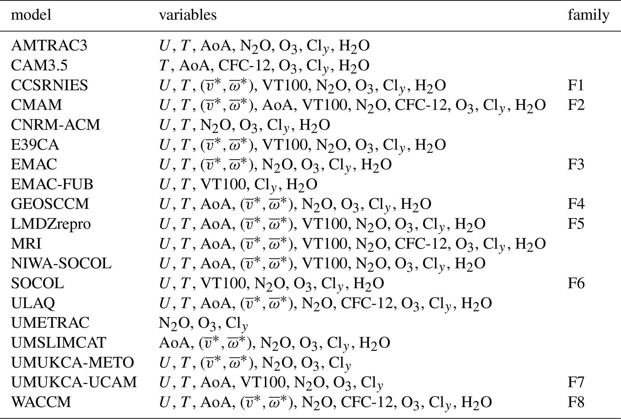
Table 2The 20 CCMI-1 models and variables used in this study.
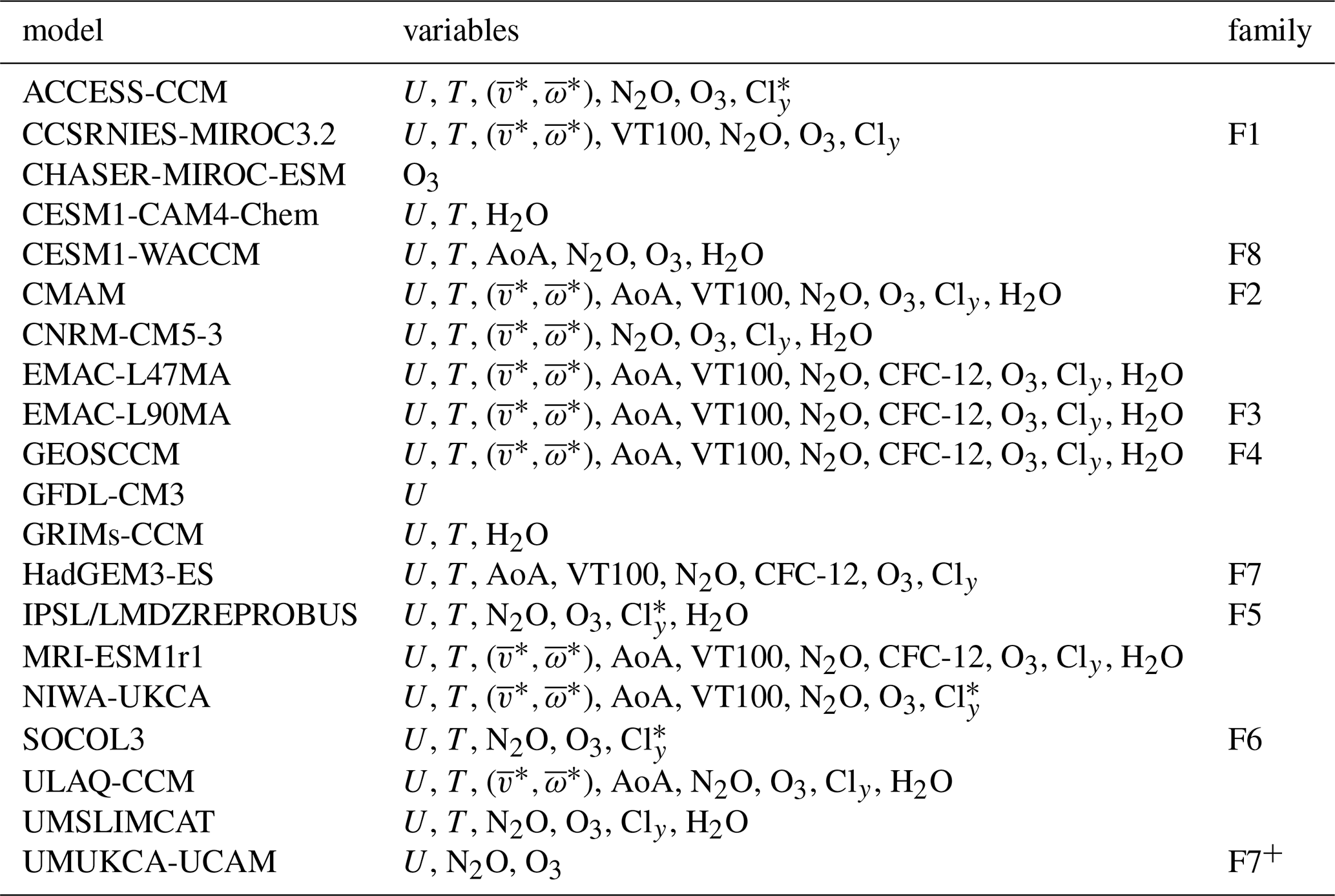
indicates Cly was archived incorrectly, but reconstructed from HCl + ClONO2 + ClO + HOCl. + UMUCKA-UCAM is used in the ozone climatology but not in the timeseries as it has unrealistic large values before 1980.
Table 3The 11 CCMI-2022 models and variables used in this study.
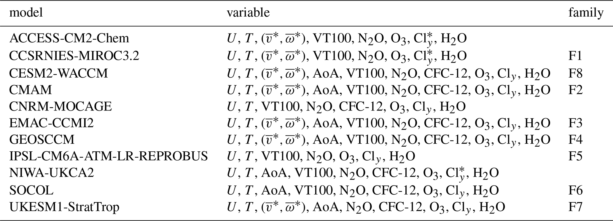
indicates Cly was archived incorrectly, but reconstructed from HCl + ClONO2 + ClO + HOCl.
2.2 Observations and reanalyses
2.2.1 Satellite observations
In parallel with the modeling advances, the availability of satellite data of chemical species has increased substantially since the SPARC (2010) report. We leverage some of the new or extended observations (MLS, MIPAS, ACE-FTS) and also merged datasets (SWOOSH, SAGE-CCI-OMPS+). We describe the specific datasets used in the following.
For N2O, we use version 5 data from the Microwave Limb Sounder (MLS) instrument aboard NASA's Aura spacecraft, which is part of the Earth Observing System (EOS)5. MLS has near-global spatial coverage (82° S–82° N), with horizontal resolution of 200–300 km along-track, 7 km across-track, vertical resolution of 3–4 km, and over 3000 profiles per day. The recommended useful vertical range is 100 to 0.46 hPa (Livesey et al., 2022). Key updates, described by Livesey et al. (2022), in the N2O version 5 compared to the earlier version 4 include a corrected instrument calibration that accounts for the slow drift in the N2O product since ∼ 2010 (discussed by Hurst et al., 2016; Livesey et al., 2021), which addresses unrealistic negative trends in N2O in the lower stratosphere, and a new retrieval method that resolves issues at the 100 hPa level seen in previous versions (see SPARC, 2017), making this pressure level now suitable for scientific use. For HCl and ClO, we use MLS level 3 data (so called ML3B data) generated by the JPL team, where daily level 2 data are averaged at 4° latitude bins using appropriate recommended filters.
We used water vapor and ozone from the Stratospheric Water and OzOne Satellite Homogenized (SWOOSH). This data set includes a merged record of stratospheric water vapor and ozone from limb sounding and solar occultation satellite measurements from 1984 to present (Davis et al., 2016). Data from four satellite sensors sensors (SAGE II/ERBS, MLS/UARS, HALOE/UARS, MLS/Aura) are homogenized for use in the merged record using coincident data taken during instrument overlap periods. We use monthly mean zonal mean data from SWOOSH on a geographic latitude and pressure grid covering 31 pressure levels from 316 to 1 hPa, although additional isentropic and equivalent latitude versions are also available. The horizontal grid used was 2.5° latitude.
For ozone, we take advantage of a second, complementary satellite dataset SAGE-CCI-OMPS+ that combines a different set of sensors using an alternative merging method. It is a monthly zonal mean ozone product developed by ESA's Climate Change Initiative (CCI) and extended regularly as part of EC's Copernicus Climate Change Service (C3S). It provides ozone concentrations and deseasonalized anomalies from October 1984 to December 2024, in 10° latitude bands from 90° S to 90° N and on a 1 km altitude grid from 10 to 50 km. The record combines measurements from nine limb and occultation sensors (SAGE II/ERBS, POAM III/SPOT-4, OSIRIS/Odin, GOMOS/Envisat, MIPAS/Envisat, SCIAMACHY/Envisat, ACE-FTS/SCISAT, OMPS-LP/SNPP, and SAGE III/ISS). The merging method essentially consists of computing the median deseasonalized anomaly of the contributing sensors and hereby differs from the method used by SWOOSH. Also, SAGE II is the only common sensor used by SAGE-CCI-OMPS+ and SWOOSH, further increasing the independence between these data records. Key algorithm, intercomparison, and trend results are documented by Sofieva et al. (2017, 2023, 2025); Godin-Beekmann et al. (2022); WMO (2022). Despite their differences in input data and merging methodologies, both SWOOSH and CCI have been shown to exhibit similar interannual variability and trends in ozone (Sofieva et al., 2025; Godin-Beekmann et al., 2022). We use both datasets here in order to demonstrate the degree of observational agreement in the context of comparisons with models.
We used N2O and SF6-derived AoA from MIPAS (Michelson interferometer for Passive Atmospheric Sounding), a limb emission interferometer that measured in the infrared on a sun-synchroneous orbit onboard the Envisat satellite from 2002 to 2012 (Fischer et al., 2008). MIPAS measured the spectrally resolved radiance of the atmosphere by pointing to dark space while looking through the atmosphere and scanning from about 70 to 7 km tangent height. The vertical scanning steps were between 1.5 and 6 km, resulting in a similar vertical resolution of the retrieval products, i.e. the global distribution of more than 30 trace gases and temperature. Here we used N2O data of spectral version 8 generated with the research processor developed and operated at the Institute of Meteorology and Climate Research (IMK), Karlsruhe Institute of Technology and Instituto de Astrofisica de Andalucia (IAA), CSIC, Granada (MIPAS-IMK in short) and described in Glatthor et al. (2024). SF6 data of spectral version 5 (MIPAS V5R-224/225) were retrieved as described in Haenel et al. (2015), however with improved spectral absorption cross sections Harrison (2020). AoA was derived from version 5 SF6 data according to the method described in Garny et al. (2024b).
N2O, CFC-12, and SF6-derived AoA are also taken from ACE-FTS (Atmospheric Chemistry Experiment Fourier Transform Spectrometer) version 3.5/3.6 (February 2004–February 2021) and version 4.1/4.2 (February 2004–present), as proposed by Saunders et al. (2025). ACE-FTS is a limb-viewing solar occultation instrument aboard the Canadian satellite SCISAT (Bernath et al., 2005). ACE-FTS measures up to 30 profiles per day with 3 km resolution, determined by the 2.5 mrad field of view, and obtains global (85° S–85° N) coverage over the course of three months. It has an orbital inclination of 74°, so the profiles are mostly concentrated in polar regions. The N2O data are from version 5.2 (Strong et al., 2008), while the SF6 used to derive AoA and CFC-12 are from version 3.5/3.6. The retrieval algorithm is described by Boone2005, with updates to v3 and v5 provided by Boone et al. (2013) and Boone (2020), respectively. The data were filtered using quality flags (Sheese and Walker, 2020) as described by (Sheese et al., 2015).
For both these instruments, the AoA datasets based on SF6 were derived using the consolidated method by Garny et al. (2024b). Briefly, this method ensures a common treatment of deriving mean age from the tracer measurements, in particular the assumptions regarding the shape of the age spectrum (e.g. the second-order moments) and applies a correction for SF6 mesospheric sinks (Loeffel et al., 2022; Garny et al., 2024a). We refer to Garny et al. (2024b) and Saunders et al. (2025) for more details on this dataset.
2.2.2 Reanalyses
For the dynamical fields, we employed data from the 3 most recent reanalyses: ERA5, JRA-3Q, and MERRA-2. ERA5 (ECMWF Re-Analysis version 5) is the latest reanalysis of the European Center for Medium-range Weather Forecasts (ECMWF; Hersbach et al., 2020). It has a horizontal resolution of ∼ 30 km (T639) and 137 levels from the surface to 0.01 hPa. Due to a known cold bias in the lower stratosphere, we have replaced data in the 2000–2006 period with the updated ERA5.1 (Simmons et al., 2020), and we denote the resulting reanalysis data ERA5/5.1. MERRA-2 (Modern-Era Retrospective analysis for Research and Applications version 2) is the latest reanalysis produced by NASA (Gelaro et al., 2017). It has a 0.5° × 0.625° latitude–longitude grid and 72 vertical levels from the surface up to 0.01 hPa. JRA-3Q (Japanese Reanalysis for Three Quarters of a Century; Kosaka et al., 2024) is the newest reanalysis produced by the Japan Meteorological Agency (JMA). It has a horizontal resolution of 40 km (TL479) and 100 vertical levels from the surface to 0.01 hPa.
Monthly mean zonal mean output of the zonal mean wind (U) and residual circulation components have been downloaded from the Reanalysis Intercomparison Dataset (RID). The RID is an updated version of the dataset “Zonal-mean dynamical variables of global atmospheric reanalyses on pressure levels” (Martineau et al., 2018), and is now provided through the JAMSTEC RID server (https://www.jamstec.go.jp/ridinfo/, last access: 18 April 2026). The dataset provides data interpolated to a common grid with 73 latitudes and 22 pressure levels up to 1 hPa. For the residual circulation components, we used an upward extension of the RID available on the RID server, adding 13 pressure levels and extending the vertical coverage up to 0.01 hPa (35 pressure levels in total). In this upward extension, unlike in the standard RID product, the variables are derived from model-level data that were interpolated to pressure levels. The residual circulation is not directly observed, and there are important uncertainties in its magnitude across reanalyses (e.g., Abalos et al., 2015; Monge-Sanz and Birner, 2022; Fujiwara et al., 2024). By considering several reanalyses, we aim to account for this uncertainty. The residual circulation has been explored for ERA5 (Diallo et al., 2021) and JRA-3Q (Kobayashi and Iwasaki, 2024), and used in some studies for MERRA-2 (e.g., Orbe et al., 2020). The cold point and lapse rate tropopauses are the version 1 of the Jülich dataset (Hoffmann and Spang, 2022; Zou et al., 2023), for the same 3 reanalyses (ERA5/5.1, MERRA-2, and JRA-3Q).
2.2.3 Chemistry Transport Model
We use total inorganic chlorine (Cly) from the global offline TOMCAT 3-D CTM (Chipperfield, 2006), which includes a detailed representation of stratospheric chemistry (Chipperfield et al., 2018; Feng et al., 2021), including heterogeneous reactions on sulfate aerosols. The model is driven by ECMWF ERA5/5.1 reanalysis winds and temperatures (Hersbach et al., 2020), with 32 hybrid sigma–pressure levels from the surface to 60 km and a horizontal resolution of 2.8° × 2.8° (Dhomse et al., 2019). The surface mixing ratios of long-lived source gases, including major greenhouse gases (GHGs) and ODSs (e.g., CO2, CH4, N2O, CFCs, HCFCs), are prescribed following the WMO 2022 scenario. Additional chlorine sources from very short-lived substances (VSLS) are included which add about 100 pptv to the stratospheric Cly budget. Solar cycle variability is prescribed using solar flux data from the NRLSSI2 model (Coddington et al., 2019), and stratospheric sulfate aerosol surface area density is taken from Luo (2016). The TOMCAT Cly is used as a reference for this important metric as satellite observational datasets do not give complete coverage of all relevant chlorine species. Thus, TOMCAT provides a guide of the expected amount of stratospheric Cly from observed surface halocarbon trends. This metric relates to a fundamental process that ozone assessment models are designed to quantify, i.e. the depletion and recovery of ozone from specified halocarbon trends. In past intercomparisons CCMs have shown a wide spread in this metric (SPARC 2010).
2.3 Diagnostics
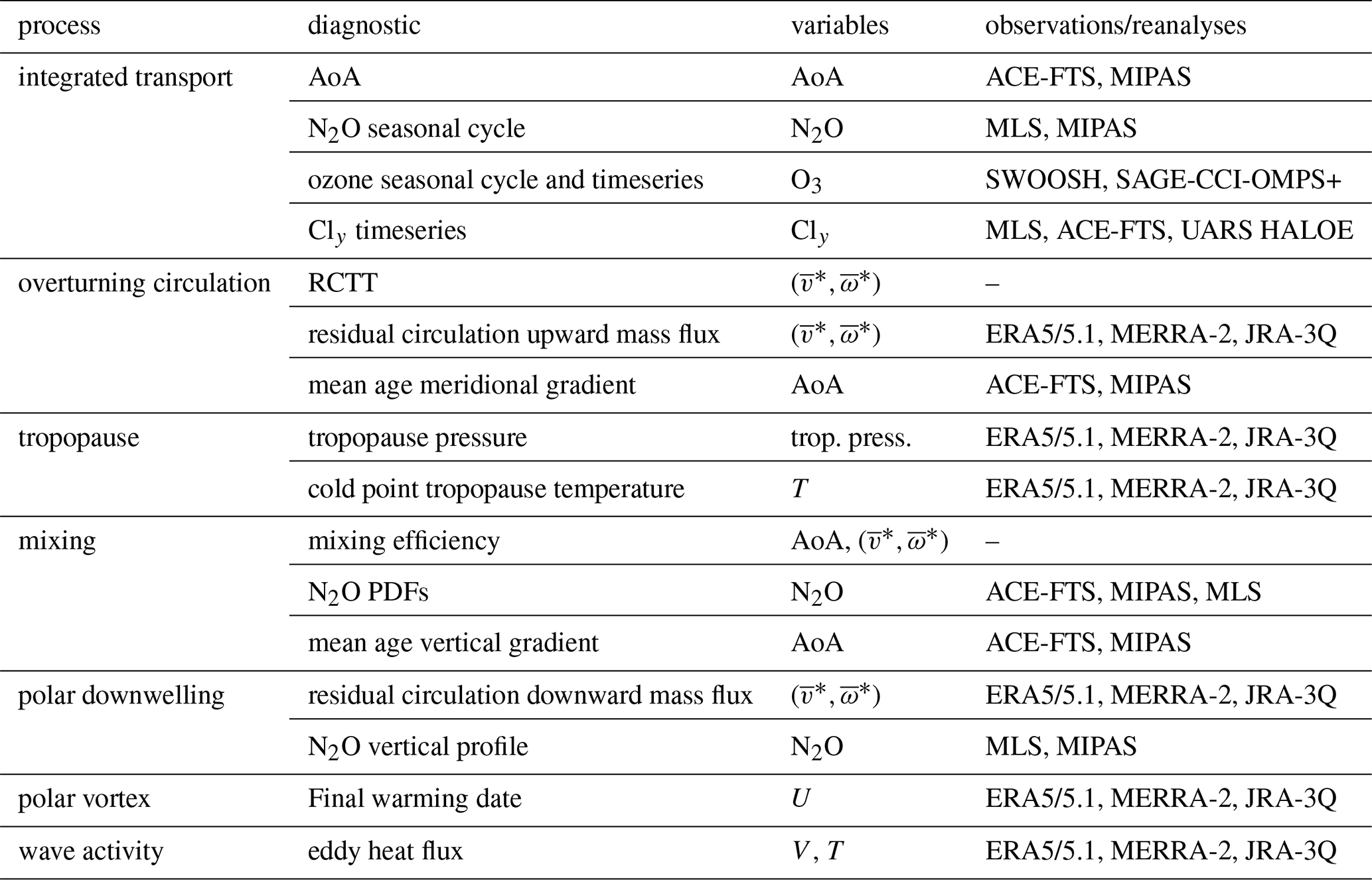
Table 4 presents an overview of the diagnostics, together with the variables needed and the corresponding observational dataset used for evaluation.
A particularly useful diagnostic to quantify the strength of stratospheric transport is the mean age of air (AoA), which measures the average time of residence of an air parcel since it entered the stratosphere through the tropical tropopause (Waugh and Hall, 2002; Garny et al., 2024b). AoA is easily represented in models and can be estimated from long-lived tracer concentrations, and it is thus useful to evaluate models against observations. The AoA includes the effects of advection by the overturning circulation and those of mixing. The tropical leaky pipe model (TLP; Neu and Plumb, 1999) provides a simplified picture of the stratosphere as a tropical region or “pipe” with ascending air, and descending air outside the pipe, with leaky barriers in between that allow for moderate amounts of mixing. The TLP model provides a useful tool for process understanding of the effects of individual processes on age of air. For example, Neu and Plumb (1999) showed that mixing across the subtropical barriers results in air reentering the tropical ascent region, thus recirculation of air masses, leading to an overall increase of mean age. Diagnostics based on the TLP model formulation were later applied to CCM and CTM data, confirming the aging effect of mixing on age in three-dimensional models (Dietmüller et al., 2018; Ploeger et al., 2015; Garny et al., 2014). Likewise, Linz et al. (2021) showed theoretically that horizontal mixing serves to increase the overall AoA while keeping the difference between AoA in the tropics and extratropics constant. Computing the time of residence that would be due exclusively to the advection by the residual circulation (RCTT), and subtracting it from the AoA gives the mean aging by mixing. However, this aging by mixing also is affected by the residual circulation through the recirculation speed. Thus, a better measure of the effects of mixing is the diagnostic of mixing efficiency, which is computed as (Garny et al., 2014):
where is the time of tropical ascent from the tropopause to a level z, with the corresponding tropical upwelling, and α is the ratio of tropical to extratropical mass. Here, following Dietmüller et al. (2018), the mixing efficiency is calculated as the best fit of Eq. (1) to the tropical profiles of AoA and from the model data over a certain height range. This metric is a gross estimation of bulk mixing properties and does not represent either vertical or temporal variations. In addition, it includes effects of vertical diffusion (Dietmüller et al., 2018).
The advective component of the BDC is typically quantified with the residual circulation in the Transformed Eulerian Mean (TEM) framework (Andrews et al., 1987). The simple Eulerian zonal mean meridional circulation does not accurately represent the actual zonal mean transport because the zonal asymmetries (eddies) dominate in the stratospheric midlatitudes. The TEM residual circulation accounts for the effects of the eddies and thus is a good approximation of the zonal mean Lagrangian circulation, while keeping the advantages of an Eulerian calculation. The residual circulation components are defined as (Andrews et al., 1987):
We convert the pressure velocity (Pa s−1) provided by models and reanalyses into vertical velocity (m s−1) by assuming a constant scale height of H=7 km. To compute the net upward mass flux of the overturning circulation, the upwelling must be integrated over the entire region between turnaround latitudes (with ), which shift seasonally towards the summer hemisphere. Making use of mass continuity, a common way of computing this is by subtracting the maximum from the minimum values of the residual circulation streamfunction (e.g. Rosenlof, 1995; Hardiman et al., 2014):
where φTASH and φTANH are the southern and northern turnaround latitudes, respectively, where the residual streamfunction maximizes (and ). We first compute the streamfunction by integrating the meridional component of the residual circulation () vertically from each level to p=0, assuming zero velocity at the top. We checked that the results remain qualitatively similar if the upwelling mass flux is computed by integrating the density-weighted vertical residual velocity between the turnaround latitudes, although the numerical values change slightly because both approaches are affected by numerical errors (not shown).
In addition to the residual circulation metrics that can only be compared with reanalyses, we include other metrics that help evaluate the strength of the advective component of the BDC against satellite observations, including an estimate of the mean global overturning circulation from the difference between age of upwelling and downwelling age (Linz et al., 2016) and an estimate of tropical upwelling from the phase propagation of the water vapor tape recorder (Mote et al., 1998).
A set of diagnostics is used to evaluate mixing between the tropics and extratropics. We examine the subtropical transport barriers (STBs) based on the probability density function (PDF) of N2O across the tropics and extratropics. N2O is a long-lived tracer widely used in stratospheric transport studies (e.g., Minganti et al., 2022; Prather et al., 2023; Dubé et al., 2023). The PDFs allow distinguishing the tropical and extratropical N2O typical values (two peaks in the frequencies), and the strong gradients formed at the edge of the surf zones, which produce a valley in the PDF between the two maxima. The separation of the two peaks and the depth of the minimum are compared to satellite results. For these calculations, the N2O monthly mean output on longitude, latitude, and pressure is first interpolated onto a common grid with potential temperature as the vertical coordinate. We checked with one model (CESM1-WACCM) that subsampling the daily model output to match the sampling pattern of the satellite observations did not modify the results substantially, except in the case of ACE-FTS due to its coarse sampling (Supplement, Fig. S13). We also checked with that model that using daily mean output instead of monthly mean does not significantly modify the results (Supplement, Fig. S12). Thus, based on these tests we decided to use the monthly mean output to reduce the computation burden. For satellite observations, we use level-2 data, as the limited sampling does not allow the monthly mean output to be representative. From the PDFs, we then identify the position of the STBs by finding the latitude that corresponds to the minimum in the PDFs, following the approach of Sparling (2000) and Neu et al. (2003). This is the only quantitative metric we present from the N2O PDFs, but qualitatively the shape of the PDF (the sharpness of the peaks and separation between them) is linked to the circulation strength and the strength of mixing. For the polar regions we include diagnostics of the polar downwelling from the residual circulation and from the N2O tendency and vertical structure. In addition, the wave activity entering the stratosphere (eddy heat flux at 100 hPa averaged over 45–75° N/S) and the final warming date are evaluated against reanalyses.
This Section evaluates the main transport diagnostics in the three generations of models. It first shows the mean age of air and decomposition into RCTT and mixing efficiency (Sect. 3.1), then addresses the BDC component due to the overturning mean meridional circulation (Sect. 3.2), then quasi-horizontal mixing between the tropics and the extratropics (Sect. 3.3). The polar processes, including polar downwelling and the polar vortex are discussed in Sect. 3.4, and finally the ozone climatology is evaluated in Sect. 3.5.
3.1 Mean age of air
We begin by showing the annual mean climatology of AoA in the three model generations and the two satellite datasets from Garny et al. (2024b) in Fig. 1. Note that throughout the paper AoA is normalized by subtracting the value at the equator and at 100 hPa in each dataset, to remove differences due to the definition of the level of zero age (some models use the tropopause, some a fixed level in the upper troposphere, some at/near the surface). It is clear that all the CCMs underestimate the AoA, especially in the extratropical middle and upper stratosphere (compare Fig. 1a–c with d–e). Also, the newest generation of models exhibits the youngest median values. Figure 1f shows the latitudinal structure of the annual mean AoA at 50 hPa, which is a classical diagnostic in stratospheric transport evaluation studies, commonly referred to as the “wing plot” due to its characteristic shape (e.g., Hall et al., 1999; Waugh and Hall, 2002; Eyring et al., 2006; SPARC, 2010; Dietmüller et al., 2018; Abalos et al., 2021; Garny et al., 2024b). This level is typically chosen because it maximizes the available in situ (balloon and aircraft) observations. Although not included in this study, we note that the in situ measurements are broadly consistent with the satellite observations and lay on the upper edge of the CCMI-2022 envelope, as shown in Garny et al. (2024b) Fig. 10 and Saunders et al. (2025) Fig. 11.
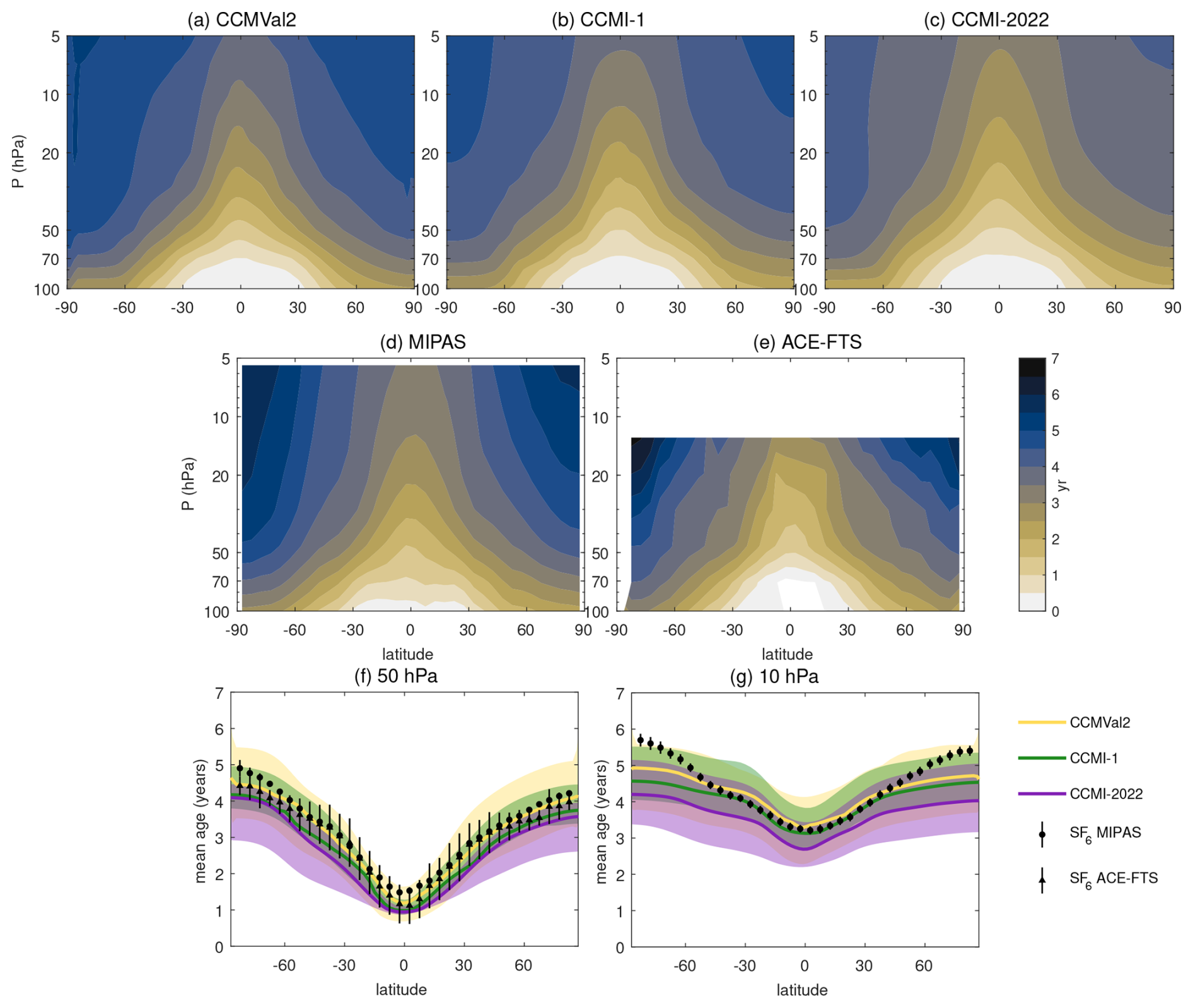
Figure 1(a–e) Cross sections (latitude-pressure) of annual mean AoA multimodel median for CCMVal-2, CCMI-1, and CCMI-2022, and for the observational dataset from MIPAS and ACE-FTS. (f–g) Latitudinal section of the mean age of air from the three generations of models and the satellite estimates at 50 hPa (left) and 10 hPa (right). In all panels the mean age is corrected by removing the value at the equator and 100 hPa of the corresponding dataset.
In all generations the spread in the mean age values across models increases with latitude, reaching up to 1.5 years in polar regions for CCMI-2022. In the tropics, the MMMed of the three generations gives an AoA of around 1 year at 50 hPa, which is in good agreement with the ACE-FTS satellite estimate. At higher latitudes, the agreement with observations decreases, and the models have a young bias throughout the extratropics. This bias is largest in the newer generation for which the observations fall on or above the upper edge of the spread. The mean age averaged globally and over 100–15 hPa is 2.3, 2.1 and 1.9 years in CCMVal-2, CCMI-1 and CCMI-2022, respectively, and 3.1 and 2.7 years in MIPAS and ACE-FTS, respectively. The young bias is more severe at upper levels, as shown for 10 hPa in Fig. 1g. This is true for all three generations, but especially again for the newest generation, which has the youngest mean age across all latitudes, with values in the polar regions that are 1.5 years younger than the observational estimate. A view of globally-integrated AoA as a function of altitude (Fig. S3 in the Supplement) confirms that the MMMed bias and the size of the inter-model spread increase with altitude. Because the mean age is an integrated transport diagnostic, the increase in bias with altitude and latitude could reflect the accumulation of transport biases as air masses ascend and move poleward through the stratosphere. It is important to note that a different number of models and different families are included in each generation. In particular, only three models provide the mean age across the three generations (CESM-WACCM, CMAM and GEOSCCM). Looking at the mean age of air wing plots for individual models across generations (see plot for common models in Fig. S2 of the Supplement) it becomes clear that there is no consistent change for the different models, with CMAM AoA staying approximately unchanged, GEOSCCM getting subsequently younger in each generation and CESM-WACCM getting younger from CCMVal-2 to CCMI-1 and then slightly older in CCMI-2022. On the other hand, the UK model family (F7 in Tables 3–3) provided mean age ouput in CCMVal-2 and CCMI-2022, and the value changed from very old (UMUCKA-UKCA) to very young (UKESM-StratTrop). Similarly, the EMAC model participated in the last two intercomparisons (EMAC-L90MA and EMAC-CCMI2), and the newer generation also shows younger age. Thus, the participation of different models in different generations does not explain on its own why the mean age has gotten younger in the new generation. Note that the shift toward a younger mean age in GEOSCCM models was recently highlighted and investigated in Orbe et al. (2025).
3.1.1 RCTT and mixing efficiency
In order to interpret the origin of the large inter-model spread in mean age, we follow the methodology of Garny et al. (2014) to decompose the mean age into a component due to the transit timescales along the residual circulation trajectories (RCTT) and a component due to mixing (see Sect. 2.3).
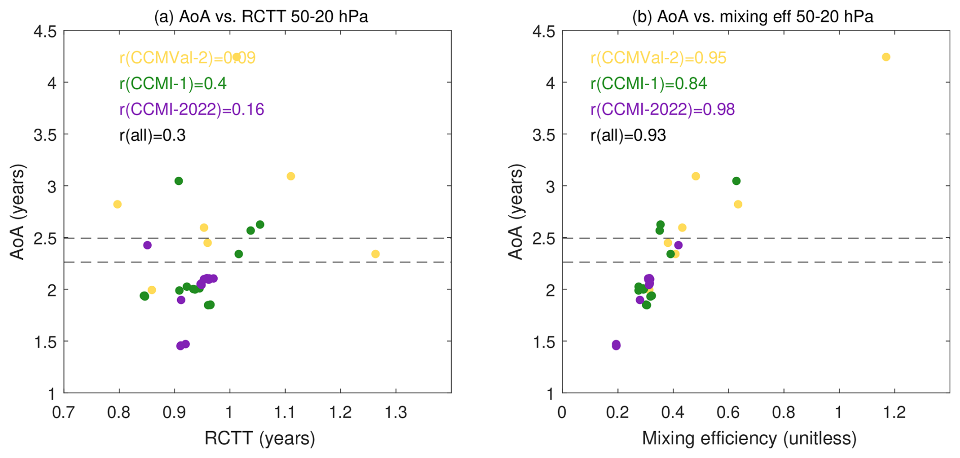
Figure 2Mean age of air versus RCTT (a) and mixing efficiency (b). AoA and RCTT are averaged over the tropics 20° S–20° N and over 50–20 hPa. Mixing efficiency is computed following Dietmüller et al. (2018). The horizontal lines show the AoA uncertainty range derived from MIPAS averaged over the same region as the models. The models included in this plot are the same included in Fig. 1. Across-model correlations of age of air and the respective diagnostic on the x-axis are given for each model generation separately, and across all model generations.
Figure 2 shows the scatter plots of mean AoA versus RCTT and mixing efficiency. Consistent with previous studies, the inter-model spread in AoA is closely related to the spread in mixing efficiency (r=0.93), while the correlation with RCTT is much weaker (r=0.3). This result is robust across model generations and reflects the importance of mixing in determining the climatological mean age simulated by a model, with a relatively small role of the residual circulation strength. In addition, the good correlation of the mean age with mixing efficiency suggests that the models simulating a tropical mean age most similar to the observations also have a more realistic mixing efficiency, while an analogous affirmation cannot be made for RCTT. This could also suggest that the generalized model bias of too young a mean age may be related to a too small mixing efficiency. Notably, the newest model generation (CCMI-2022) exhibits the lowest mixing efficiencies, consistent with its largest bias towards too young mean age of air. A mixing efficiency that is too weak in the lower stratosphere means air does not recirculate as much at those levels, causing a young bias throughout the stratosphere (cf. Neu and Plumb, 1999; Garny et al., 2014; Linz et al., 2021). Nevertheless, we emphasize that these results could also indicate excessive vertical diffusion in the models (Dietmüller et al., 2018).
In summary, the mean age is underestimated in the CCMs, especially in the newest generation. The large spread in mean age values is correlated with the spread in mixing efficiency. These two are consistent: the young ages in the newest generation would be expected with weaker mixing efficiencies, which could likely reflect excessive vertical diffusion.
3.2 Advection by the mean meridional overturning circulation
We now explore in more detail the advective component of the BDC, the mean meridional overturning circulation. As described in Sect. 2.3, we compute the net upward mass flux to account for the fact that the region of tropical upwelling is not fixed but moves seasonally towards the summer hemisphere.
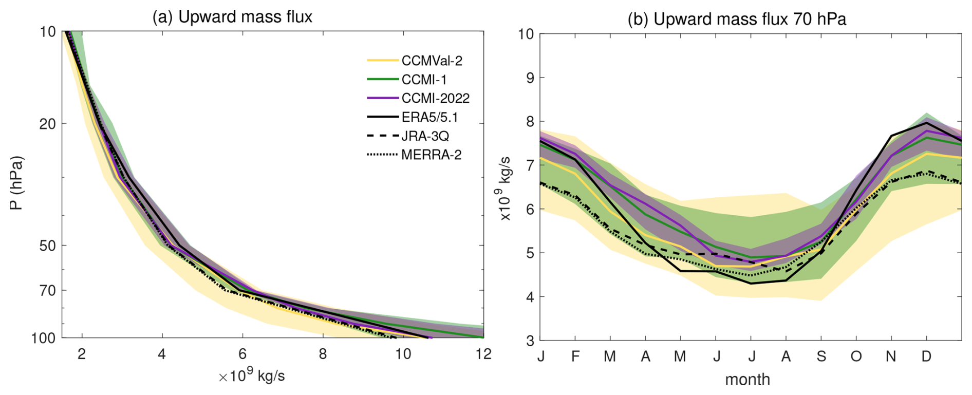
Figure 3Net upward mass flux in the three model generations (MMMed and 15th/85th percentiles) and three reanalyses (ERA5, JRA-3Q, MERRA-2). (a) Annual mean vertical structure (b) seasonal cycle at 70 hPa.
Figure 3a shows the vertical profile of the annual mean upward mass flux from the tropical tropopause to the middle stratosphere. The mass flux in our observation-based references, the reanalyses, decreases rapidly with height due to the exponential decay of air density, with values around 10 × 109 kg s−1 at the tropopause decreasing to 1.5 × 10⁹ kg s−1 at 10 hPa. However, there is a clear difference between the reanalyses, with ERA5/5.1 exhibiting larger values than the other two reanalyses below 20 hPa. The CCMs are generally able to capture the mean vertical structure of the overturning mass flux seen in the reanalyses. In the range 50–20 hPa, where ERA5 shows larger values than the other two reanalyses, the models agree better with MERRA-2 and JRA-3Q. Below 50 hPa, in contrast, the models agree better with the higher values found in ERA5/5.1. In this lower stratosphere region, MERRA-2 and JRA-3Q are outside the inter-model spread range of the models for the last two generations (CCMI-1 and CCMI-2022). The oldest generation (CCMVal-2) shows a wider spread, which includes all reanalyses.
Figure 3b shows the seasonal cycle in the net upward mass flux in the lower stratosphere (70 hPa). The difference between ERA5/5.1 and the other reanalyses is concentrated in the boreal winter months (November to March), overall leading to a larger amplitude in ERA5/5.1's seasonal cycle. Across the three generations, the models MMMed show a larger seasonality (∼ 40 %) compared to MERRA-2 and JRA-3Q (∼ 30 %), although still smaller compared to ERA5 (∼ 50 %). The inter-model spread is largest throughout the year in the oldest generation (CCMVal-2), and notably reduced in the newest generation (CCMI-2022), although the MMMed is very similar to that from the previous generation (CCMI-1). As will be shown, the reduced spread is a common feature of the newest model generation found across several metrics (but not in all). At higher levels, the annual cycle is reduced (with the semi-annual variability becoming dominant, e.g., Abalos et al., 2021) and the agreement between model generations and reanalyses increases as the magnitude becomes smaller (Fig. S5 in the Supplement).
As mentioned in Sect. 2.3, an alternative way to derive the mean meridional overturning circulation that enables direct comparison with satellite data is based on age and the TLP model. This method has a the advantage of being an estimate of the overturning circulation that is independent from the residual circulation mass flux estimate in Fig. 3. On the other hand, there are important caveats associated with this observational estimate, as will be discussed below. Previous studies have shown that the difference in mean age between the tropics and the extratropics in isentropic coordinates is inversely proportional to the mean strength of the overturning circulation, and does not depend on mixing (Linz et al., 2016).
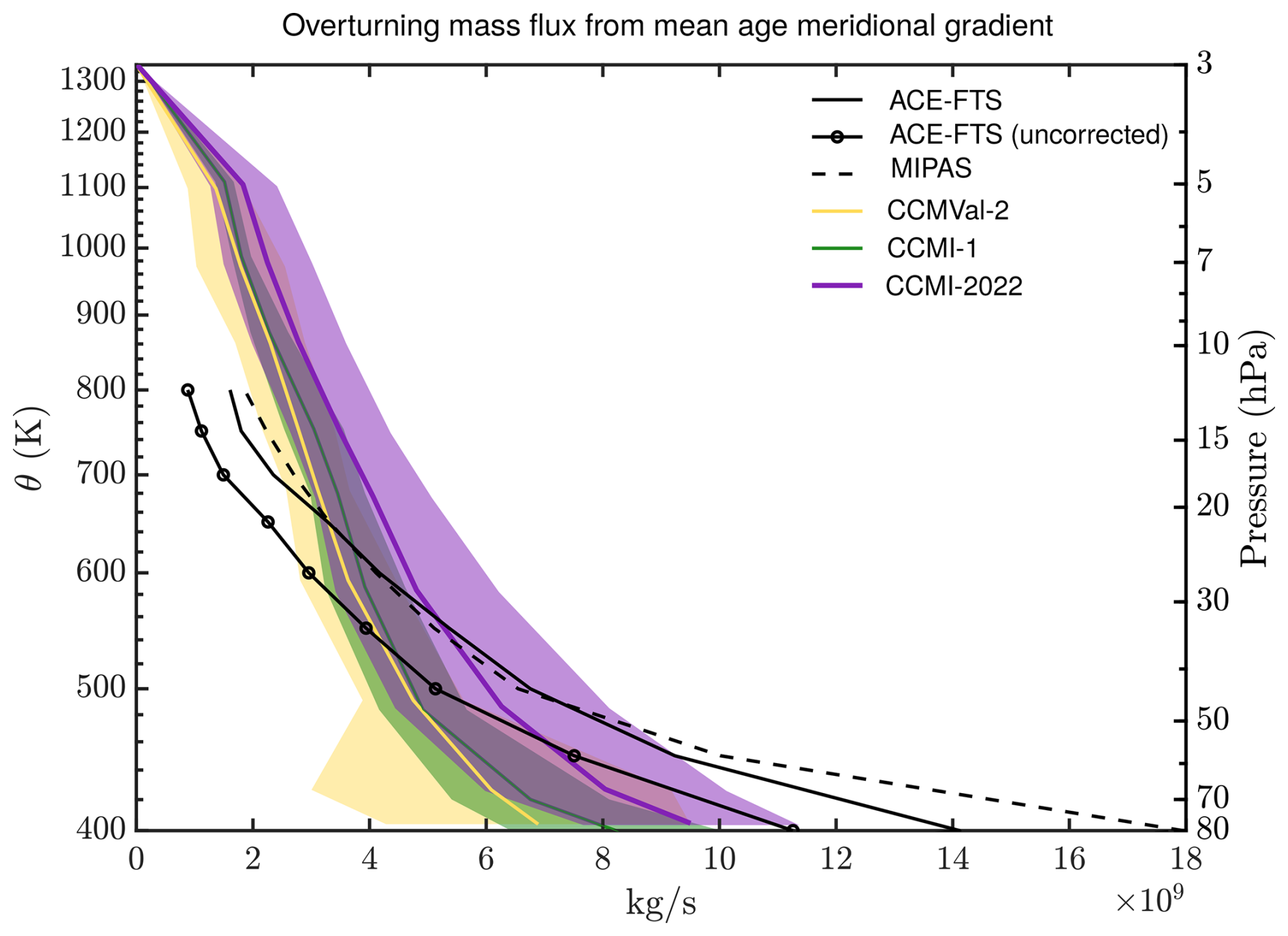
Figure 4Estimate of the mean meridional overturning mass flux from the meridional mean age gradient following Linz et al. (2016). Calculations shown for ACE sink-corrected, ACE uncorrected, and MIPAS data and for the multi-model median of the three generations of models, where the shading represents the median absolute deviation at each level. The second y-axis shows the CCMI-1 pressure for comparison with other metrics in this study.
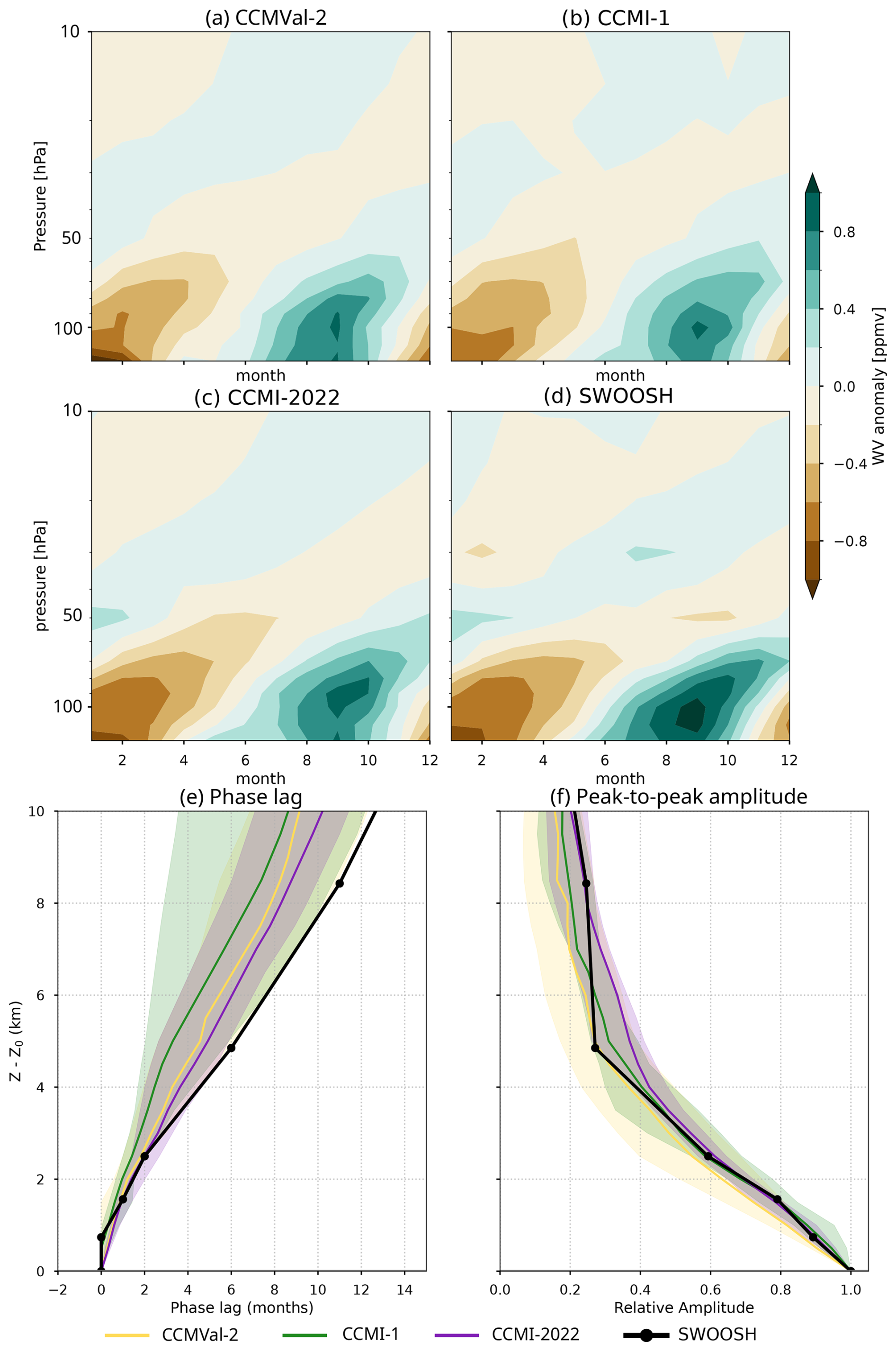
Figure 5(a–d) Water vapor tape recorder signal (20° S–20° N) in tape recorder in CCMVal-2, CCMI-1, and CCMI-2022 multi-model medians and SWOOSH. The time period over which the tape recorder is computed starts in 1992 for all datasets and ends in 2005 for CCMVal-2, 2012 for CCMI-1, and 2018 for CCMI-2022 and SWOOSH. (e–f) phase lag (e) and amplitude (f) as a function of distance from the level of peak tape recorder amplitude.
Figure 4 shows this age gradient metric computed from the mean age output for the three generations of models and estimated from the satellite-based mean age data (Garny et al., 2024b). The metric is computed on isentropic levels, but approximate corresponding pressure levels are also given for reference. While the mass flux values are broadly consistent with those in Fig. 3, this simplified estimate shows a substantially larger spread (e.g., 3 × 10⁹ kg s−1 near 70 hPa for CCMI-2022, which corresponds to almost 50 % of its magnitude). The newest generation shows larger values throughout the altitude range, which is not observed in Fig. 3a. These differences between the mean meridional overturning circulation results are not due to the fact that different models provide residual circulation and mean age output (Figs. S1 and S4). Rather, they are likely due to the very different approaches, variables and calculations involved in each method. A comparison between residual circulation and age gradient mass flux was carried out in Linz et al. (2019), but was based on variability, not climatology. The observational age gradient mass flux estimates suggest that the models' overturning circulation is too fast above ∼ 40 hPa, and too slow below that level. This result is also at odds with that derived from reanalysis mass flux (Fig. 3), which suggests an overestimation only in the lower stratosphere. However, there are important observational caveats to consider. As shown by Saunders et al. (2025) (see their Fig. 11), at 50 hPa, the difference in mean age between tropics and extratropics is too small for the age derived from SF6 with the mesospheric sink correction for both MIPAS and ACE-FTS estimates, compared to in situ observations. This is because the MIPAS mean age is biased high (old) in the tropics relative to in situ observations and agrees well in the extratropics, while the ACE-FTS mean age is biased low (young) in the extratropics, and agrees well in the tropics. This leads in both datasets to a lower meridional gradient in mean age and thus an overestimated overturning circulation. The ACE-FTS non-corrected for SF6 approximates better the gradient suggested by in situ measurements (Fig. 11 of Saunders et al., 2025), and using these values, the curve is more consistent with the model output in the lower stratosphere (below ∼ 30 hPa, see Fig. 4). However, at the upper levels, this results in lower values that fall outside the model range, as expected, since the influence of the mesospheric sink of SF6 on the age calculation should increase with altitude. Hence, we conclude that this metric should be considered with care, given the observational limitations. An additional potential source of discrepancy is the temperature and static stability biases in the models, which result in shifted isentropic levels and their thickness relative to reanalyses. Overall, our analyses show that the overturning mass flux estimate from the age gradient should not be directly compared to residual circulation-based diagnostics.
An additional estimate of tropical upwelling in the lower stratosphere can be obtained from the tape recorder signal imprinted by the seasonal cycle in cold point temperature (Mote et al., 1998). The dry and wet anomalies imprinted by the larger dehydration in boreal winter as compared to summer propagate upward with the residual circulation, and thus the phase lag between different levels can be used as an estimate of the upwelling strength. The tape recorder signal is captured by most models, though with very different amplitudes and upward propagation rates (Supplement Figs. S5–S7). Figure 5a–d shows the MMMed tape recorder signal in the three generations, and the SWOOSH satellite dataset results for comparison.
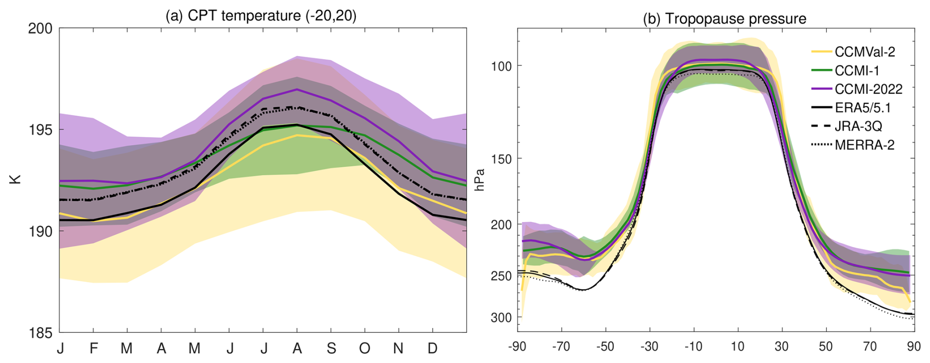
Figure 6(a) Annual cycle of the cold point tropopause temperature averaged over the tropics (20° S–20° N) for the multi-model median and MAD of the three generations and three reanalyses. (b) Annual mean lapse rate tropopause pressure as a function of latitude.
The MMMed of the three generations shows a consistent tape recorder signal with weaker amplitude compared to SWOOSH, but there is a very large spread across individual models. The MMMed amplitude is larger and thus more realistic in the new generation. For a quantitative comparison of the MMMed and the inter-model spread, Fig. 5e shows the phase of the tape recorder as a function of altitude relative to the maximum amplitude of the tape recorder anomalies (near the cold point tropopause) up to 10 km above the peak amplitude (corresponding to ∼ 25 hPa). Compared to the observations, the models generally capture the speed of the ascent above the tropopause, although most models tend to carry the anomalies upward too fast (shorter phase lag for a given level), especially higher than 3 km above the maximum tape recorder amplitude (∼ 66 hPa). This estimate thus provides independent qualitative support for the result obtained with the upward mass flux of the residual circulation, that upwelling is overestimated in the models, although the tape recorder diagnostic suggests that this bias extends to higher levels. It is important to keep in mind that this metric does not provide a clean measure of advection by tropical upwelling, as it includes the effects of vertical and horizontal mixing and diffusion (Mote et al., 1998; Glanville and Birner, 2017). We will discuss the information on horizontal mixing that can be extracted from the tape recorder referring to Fig. 5f in the next section. Note that the newest model generation has the smallest spread and closest values to the observations. Finally, we note that the results might also depend on the rate of methane oxidation and its increase with altitude, which might be different across models.
The amount of water vapor that enters the stratosphere is controlled by the temperature of the cold point tropopause (CPT). Figure 6a shows that the seasonal cycle of the CPT temperature is overall captured by the models, consistent with the reasonable MMMed tape recorder signal in Fig. 5, but with a very large spread across models in the absolute values (up to 5 K). Note that ERA5/5.1 has a colder CPT compared to the other reanalyses (by ∼ 1 K), consistent with the faster tropical upwelling seen in Fig. 3. In addition, there is a warm bias of 1–2 K in the newest generation multimodel median, although the seasonality is better captured than in previous generations. The lapse rate tropopause is too high in the models, especially in the extratropics, where there differences across models are largest (Fig. 6b). This issue has thus persisted since the CCMVal-2 intercomparison by Gettelman et al. (2010). In the tropics, the newest generation has the highest tropopause.
3.3 Mixing
The other major component of tracer transport, in addition to advection by the mean meridional overturning circulation, is mixing. As mentioned in the Introduction, strong quasi-horizontal mixing occurs in the surf zone in the extended winter of each hemisphere and is the main transport mechanism in that region, while the slow ascent is dominant in the tropical stratosphere. The transition between these two different regions and transport regimes can be visualized by plotting the probability density functions (PDFs) of a long-lived tracer such as N2O across tropics and midlatitudes.
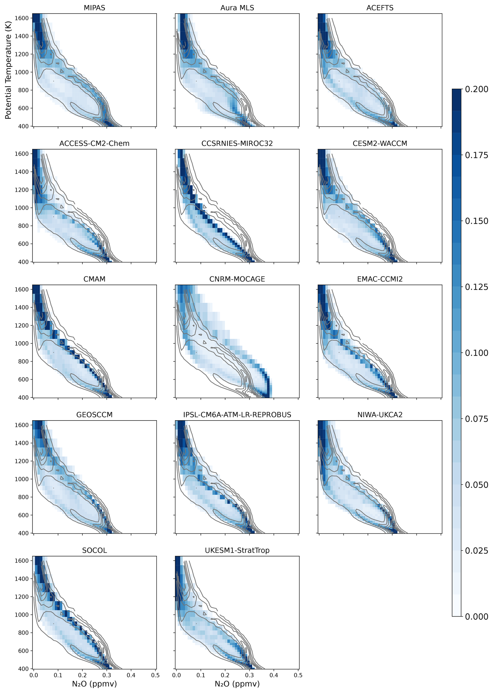
Figure 7PDFs for N2O satellite data from MIPAS, MLS, ACE-FTS (top panels), and monthly mean model data from CCMI-2022 models. 10° S–45° N, MAM season 2005–2012 period. The ACE-FTS PDF contours are shown in all panels to facilitate the comparison (gray contours). The tracer mixing ratios are binned in 100 bins in the range 0–0.5 ppmv, and the PDF is normalized such that the total frequency on each level adds up to 1.
Figure 7 shows the PDFs of N2O as a function of potential temperature for various satellite datasets (MIPAS, MLS, ACE-FTS; top panels) and the individual CCMs from CCMI-2022 in boreal spring, following SPARC (2010). The altitude range corresponds approximately to 80–1 hPa. The PDFs show two separate branches that are distinguishable between ∼ 450 to 1200 K, which correspond to the tropical and extratropical mixing ratios (the tropical pipe and the surf zone), which can be considered well-mixed. Between these two modes, there is a minimum in the PDF which corresponds to the steep gradients created at the equatorward edge of the surf zone, which reveals the presence of a subtropical mixing barrier. The three observational datasets present strong similarities, although the details are different. The most notable difference is that MLS presents an unrealistic step-like behavior below 800 K (∼ 10 hPa), likely due to a localised high-bias in N2O at this level compared to these other instruments (SPARC, 2017). The results for the SH are similar, with models maintaining the sign of the bias in both hemispheres and across generations (Supplement Figs. S14–S18). For example CCSRNIES-MIROC has too small a distinction between the branches and GEOSCCM has too large tropical values (Supplement Fig. S18). In order to compare the distributions more quantitatively, Fig. 8a,b shows the PDFs at the level of 600 K (∼ 30 hPa). The N2O concentrations have been normalized by removing the mean for each dataset to facilitate analysis of the key features beyond the mean bias, which are peak-to-peak separation and the depth of the minimum.
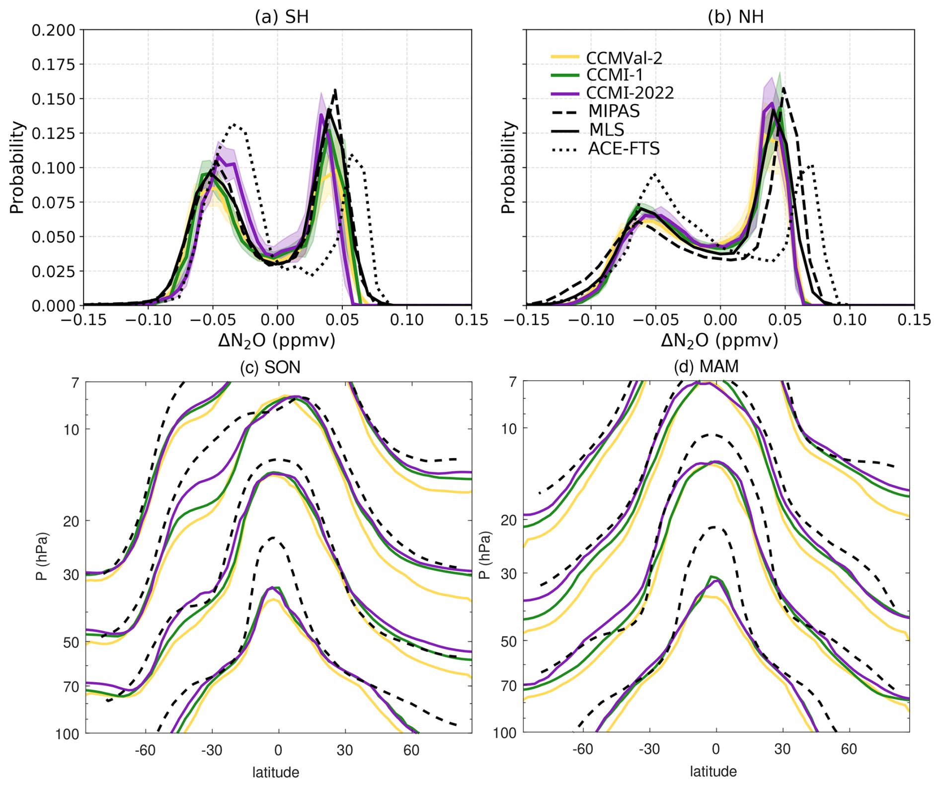
Figure 8(a–b) PDF profiles for MMMed for the three generations with observations at 600 K, 2005–2012. Each model's PDF is shifted so its mean mixing ratio aligns at zero. (c–d) Contours of N2O mixing ratio for the MMMed of the three generations and MIPAS (contour levels: 0.07, 0.014, 0.021 and 0.028 ppmv; values decrease with altitude). 1990–2010 mean for models and 2005–2012 mean for observations.
The double peak structure is apparent in all observational datasets, but ACE-FTS shows substantial deviations from the other two datasets, both in the magnitude and location of the peaks. Keeping in mind that this satellite has a much sparser sampling, as well as the agreement between the other two datasets, we compare the models against MLS and MIPAS. Note that removing the mean takes care of the MLS shifted behavior in the lower stratosphere seen in Fig. 7. In both hemispheres, the MMMed of CCMI-2022 tends to place the maxima too close together, as identified in most models in Fig. 7. On the other hand, the depth of the minimum is generally well captured by the MMMed in all model generations, although it is slightly less pronounced, which could reflect a smoother transition from the tropical to the extratropical regimes. From the minimum in the N2O PDF, we derive the position of the subtropical mixing barriers (Supplement Fig. S21). We find that the three multimodel medians are remarkably close to the observations, and indeed, the intergenerational spread in the median values is smaller than the difference between the two observational datasets (MIPAS and MLS). The spread is larger in the NH (originating in JJA, not shown), and is reduced in the newest generation.
Figure 8c, d shows the climatological N2O contours for the MMMed of the three generations and MIPAS. There is an overall low bias in CCMI-2022 N2O mixing ratios compared to MIPAS (isopleths are located at lower levels), as mentioned regarding Fig. 7. In the tropics, this bias maximizes near 20 hPa, such that the decline of N2O with altitude is too steep in the lower stratosphere (Fig. S20 in the Supplement). This could reflect overestimation of horizontal mixing. The sharp transition between tropical and extratropical N2O concentrations is smoothed out in the models' MMMed compared to the observations, consistent with the PDF behavior (the two peaks are closer together and the minimum is less pronounced in Fig. 8a–b). Note that the models represent the midlatitude plateau (surf zone) and the tropics-extratropics transition more accurately in the SH spring than in the NH spring.
Previous studies have proposed a metric for the tropics-extratropics mixing strength derived from the TLP model. Specifically, the vertical gradient in tropical mean age can be related with the mixing strength (Linz et al., 2021). Qualitatively, this can be understood by considering the fact that mixing from the extratropics into the tropics makes tropical air older, and so the vertical gradient is related to mixing. There are two main caveats about this; the same caveats about satellite data biases as with the meridional age difference above and the fact that the metric treats the extratropics as well mixed, leading to apparent negative mixing efficiencies at higher levels. Nevertheless, we show this metric in Fig. 9.
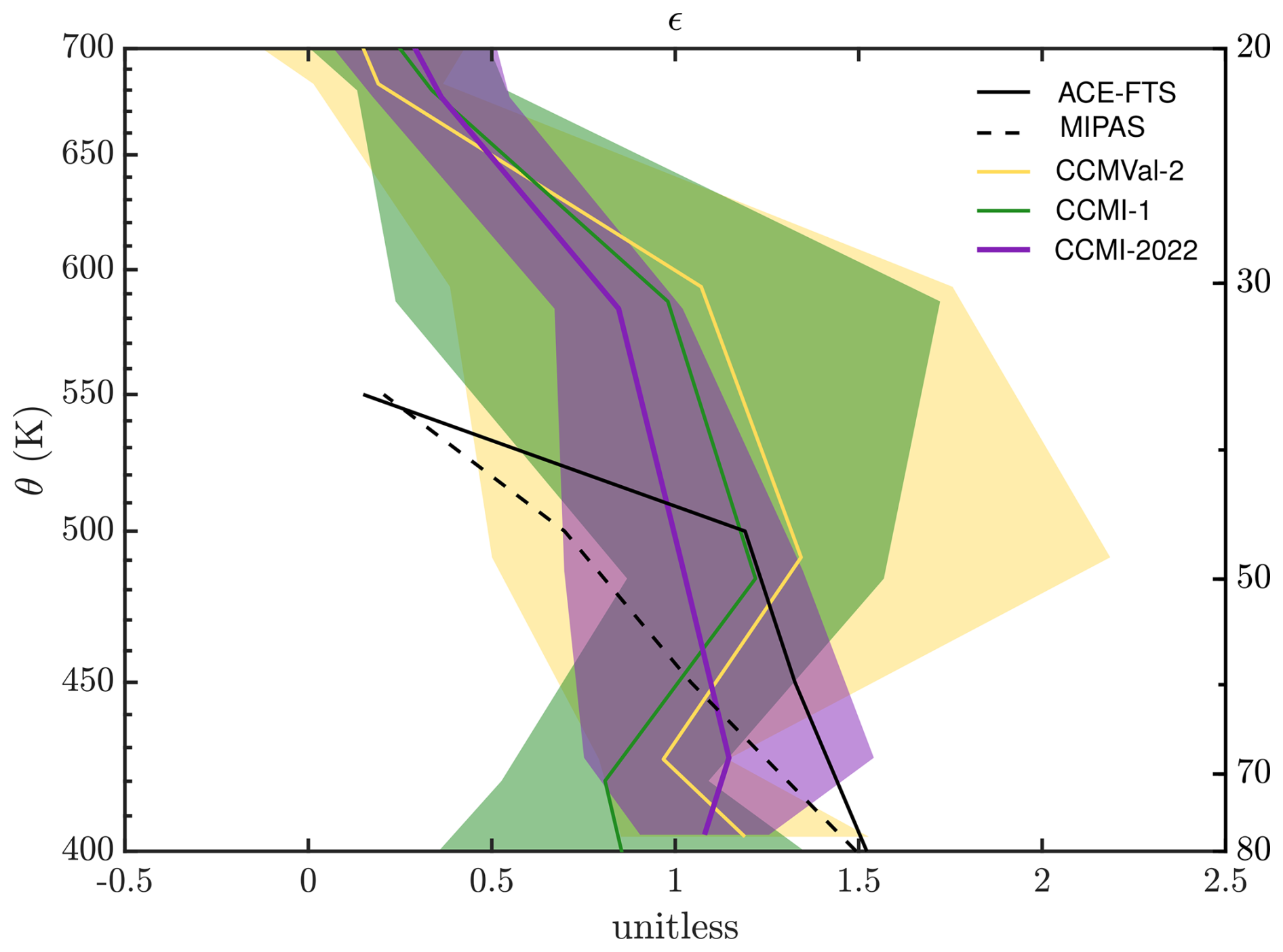
Figure 9Mixing efficiency calculated following Linz et al. (2021) is shown for ACE-FTS sink-corrected and MIPAS data. Calculations are also shown from CCMVal-2, CCMI-1, CCMI-2022 models, where the shading represents the median absolute deviation at each level. The right vertical axis shows the CCMI-1 pressure for comparison with other metrics in this study.
We note that there is non-negligible observational uncertainty, as evidenced by the difference between the two satellite-derived products. The models generally agree across generations within the large uncertainty given by the intermodel spread, with the newest generation having the smallest spread. The model values generally agree with the observational estimates below ∼ 500 K (∼ 40 hPa), although there is evidence that their mixing is too weak in the lower stratosphere (below 450–500 K, depending on the observational dataset considered). Between 500–550 K the models overestimate mixing, but note that above this level, the well-mixed assumption invoked by the mixing strength theory in Linz et al. (2021) breaks down and observed estimates for mixing efficiency are negative: these points have been removed. The models' mixing efficiency remains positive throughout the range of isentropes presented in Fig. 9, suggesting that the models remain well mixed through a deeper depth of the stratosphere than the observations. To summarize, while there is overall agreement in the lower stratosphere, with some suggestion of too weak horizontal mixing below ∼ 50 hPa, the observational uncertainty is too large to constrain the models. Finally, similar to Fig. 2, this could instead be reflecting too large vertical diffusion (Dietmüller et al., 2018).
An additional metric for the horizontal mixing can be provided by the damping of the water vapor tape recorder signal, as this damping is due to mixing with extratropical air. Figure 5f shows the peak-to-peak amplitude of the tape recorder signal as a function of height. There is a substantial spread in the damping of the tape recorder across models, which is reduced in the newer generation. Overall, it appears that most models in CCMI-2022 damp the signal too slowly with altitude around 5 km above the tropopause (∼ 50 hPa), which implies that they tend to underestimate the mixing with the extratropics. However, this result is inconsistent with the N2O analyses, which show too smooth tropics-extratropics transitions and too strong vertical gradients in the tropics, both compatible with strong mixing. The weak tape recorder damping could also be caused by an excessive vertical diffusion in the models extending the anomalies upward; another possibility could be too fast methane oxidation in that region.
In summary, different metrics of mixing do not provide a consistent picture of mixing biases in models. While there is some evidence from the tape recorder and the vertical age gradient metrics of an underestimation of mixing between the tropics and extratropics in the lower stratosphere in CCMs, which is broadly consistent with the low mixing efficiency associated with the young bias in mean age of air (Fig. 2), the N2O structure suggests an overestimation of mixing. These discrepancies could be reflecting other effects such as excessive vertical diffusion or methane oxidatoin in the models, or could be due to limitations in the tracer representation from satellite observations.
3.4 Polar processes
We now turn to the polar regions, which feature a distinct transport regime characterized by the isolation from the middle latitudes by the polar night jet and the polar downwelling of the deep branch of the mean meridional overturning circulation. Figure 10 shows the annual cycle of total polar downwelling mass flux in the two hemispheres at 30 hPa, computed from the maximum of the streamfunction for the NH and the minimum for the SH.
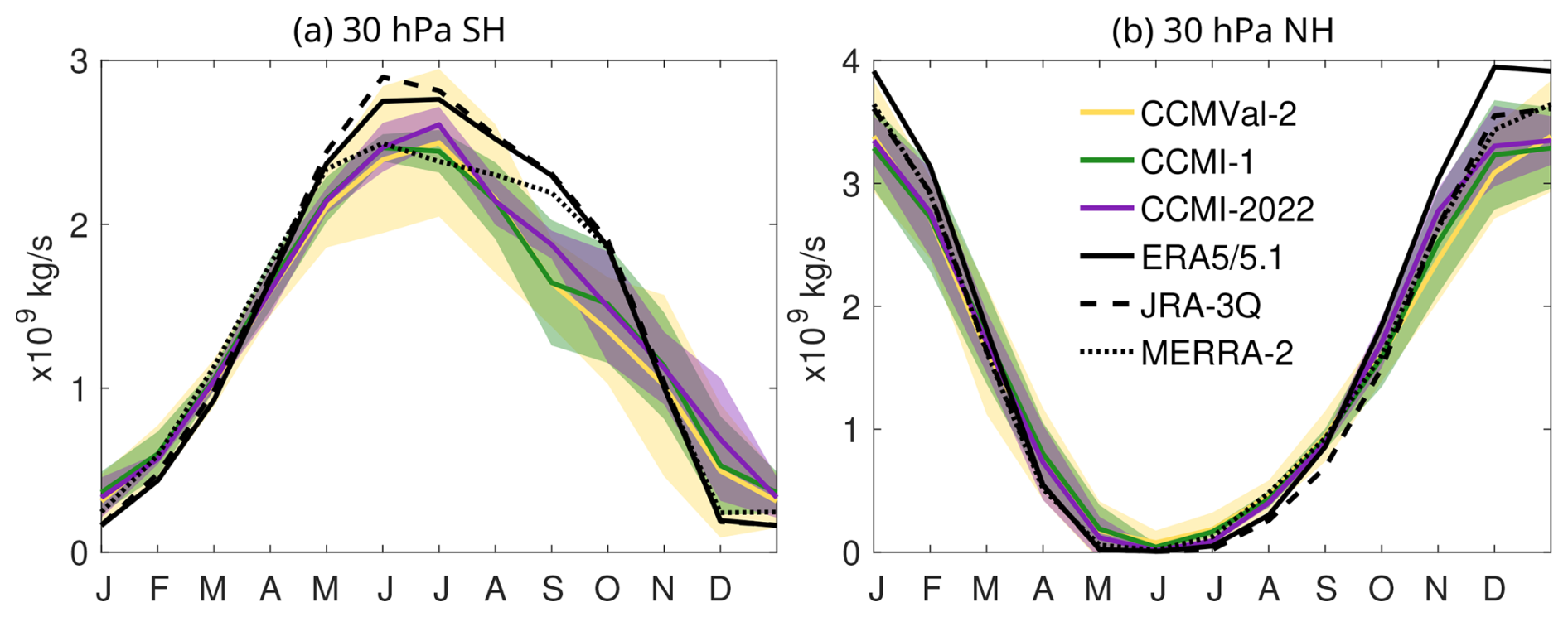
Figure 10Seasonal cycle of the SH (a) and NH (b) polar downward mass flux in the three generations together with reanalyses estimates (ERA5/5.1, JRA-3Q, MERRA-2). Shading shows the 15th and 85th percentiles.
The most outstanding feature is that in the SH, the models have too weak downwelling compared to reanalyses, especially in spring (September–October). In December, the bias is reversed, and all models overestimate downwelling, which is at its minimum in the reanalyses. This behavior in December could reflect the delayed breakdown of the polar vortex that will be discussed below. The NH downwelling shows better agreement and a smaller inter-model spread, with a slight underestimation of the maximum downwelling in December–January, especially compared to ERA5. These results are consistent across model generations.
Polar downwelling is responsible for the downward transport of air masses and tracers in the polar stratosphere. In particular, for a tropospheric-origin long-lived tracer such as N2O, polar downwelling reduces its concentrations in the lower stratosphere (Minganti et al., 2020). Consistently, the N2O tendencies are negative in the extended winter, reflecting the influence of polar downwelling. Figure 11a–b shows the seasonal cycle of N2O monthly tendencies in both hemispheres in the model results and satellite observations from MIPAS and MLS. In the SH, both observational datasets show a pronounced minimum in September-October, which is not captured by the models. This missing negative tendency is most likely related to the weak downwelling in these months found in Fig. 10. In the NH, the winter negative tendencies peak in December and are generally better captured by the models compared to the SH.
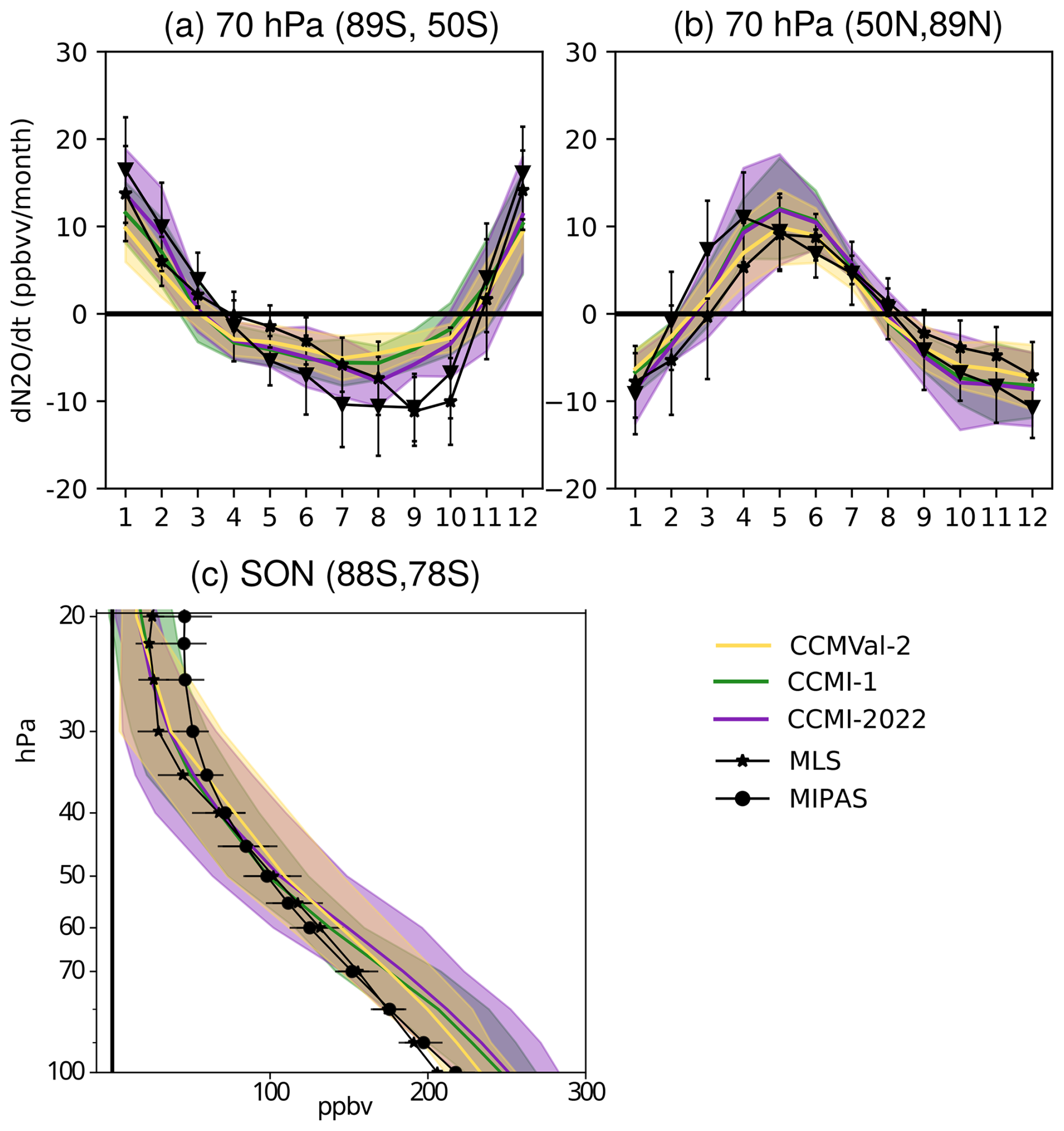
Figure 11(a–b) Climatological seasonal cycles of the N2O tendency (ppbv per month) at 70 hPa for the southern extratropics (a; 89–50° S), and the northern extratropics (b; 50–89° N). MLS and MIPAS use their respective complete periods. All models show 20 years: 1980–2000 for CCMVal-2, 1990–2010 for CCMI-1 and 1998–2018 for CCMI-2022. (c) Vertical profile of N2O mixing ratios (ppbv) in the climatological SON season over the southern polar region (88–78° S).
In spring and summer, high latitude N2O increases as the polar vortex barrier disappears, allowing for enhanced mixing with N2O-rich air from lower latitudes. The positive tendencies in spring and summer are reasonably well represented in the model results. In the NH, MIPAS suggests an earlier increase of N2O compared to MLS and to the model results, placing the maximum tendency one month earlier (March instead of April). To test if this difference could be due to the different periods covered, which includes years with sudden stratospheric warmings, we repeated the analysis for the common period, but obtained similar results. Another possibility is the different coverage of the polar region by both instruments. The seasonality in the model results agrees best with the MLS seasonality, which has a better spatio-temporal coverage. In both hemispheres, the inter-model spread is comparable to the observational uncertainty.
In order to further explore the impact of the weak polar downwelling in the SH spring, Fig. 11c shows the vertical profile of polar N2O mixing ratios in SON in model results and satellite observations. The mixing ratios of N2O in the lower stratosphere (below ∼ 60 hPa) are substantially larger in the model results than in the observations, which is consistent with the weak polar downwelling found in all generations in Fig. 10. Note that in late spring, the polar vortex can break and increase substantially horizontal mixing, which increases the N2O mixing ratios in the polar region. Nevertheless, we will show below that this increased mixing happens too late in the models on average, and thus it is likely not contributing to the larger N2O mixing ratios in SON.
The downwelling of the residual circulation is associated with the Coriolis torque exerted by the wave drag from the dissipation of planetary Rossby waves (resolved by the models) and gravity waves (parameterized in the models). The wave drag also decelerates the polar vortex. A common diagnostic of the resolved upward wave activity flux entering the stratosphere (which will then dissipate at some point and drive the residual circulation) is the midlatitude eddy heat flux at 100 hPa, as it is the dominant term of the vertical component of the Eliassen-Palm flux (Andrews et al., 1987). Figure 12 shows this diagnostic applied to the model results and reanalyses.
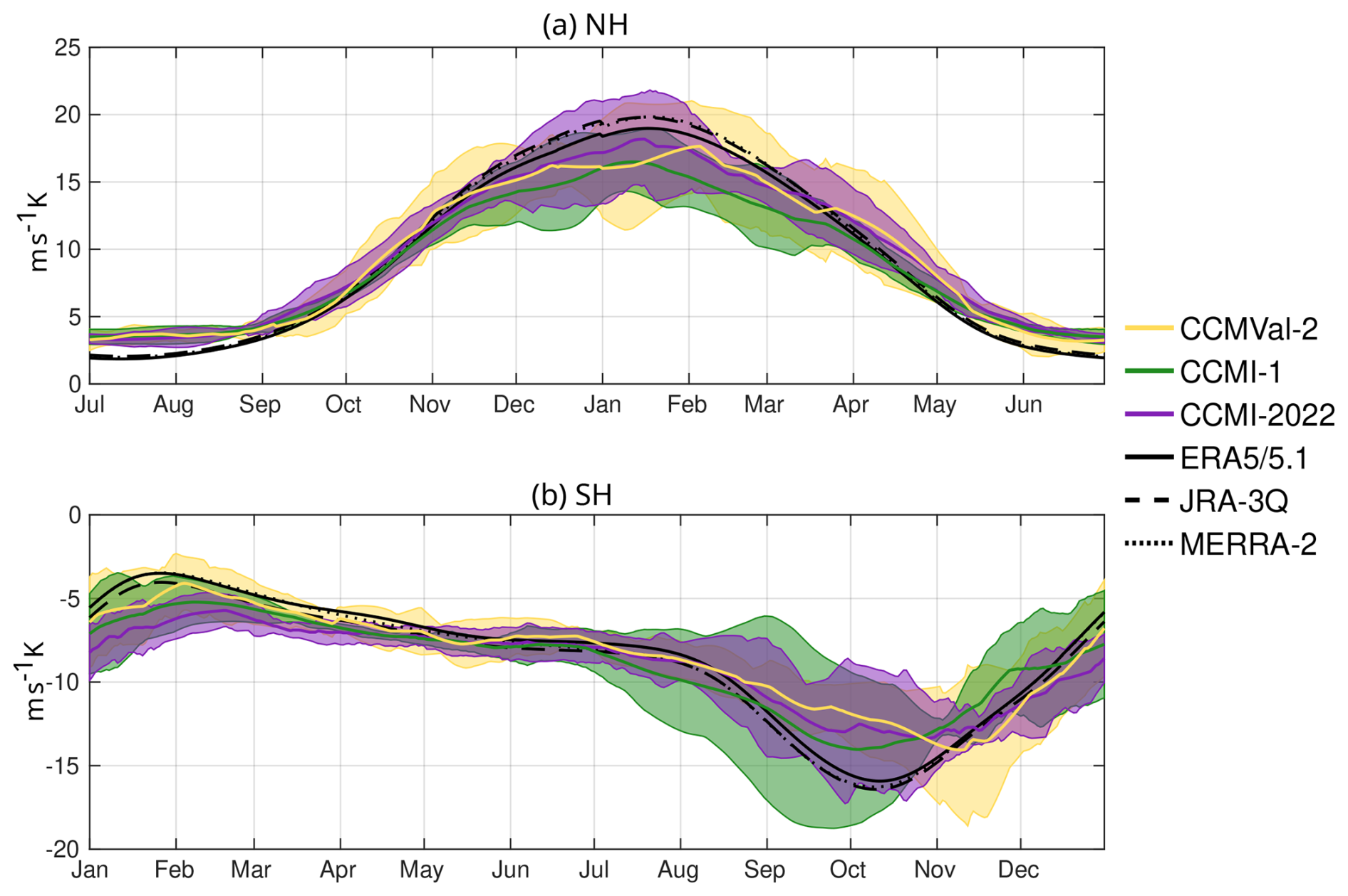
Figure 12Annual cycle of the eddy heat flux at 100 hPa averaged over the latitude band 45–75° in the NH (a) and the SH (b). Note that positive fluxes in the NH and negative fluxes in the SH both indicate poleward eddy heat transport and and upward wave propagation.
There is good agreement for the NH eddy heat flux between the model and reanalysis results, although the models tend to slightly underestimate the mid-winter maximum, especially in CCMVal-2, and overestimate the summer minimum. In the SH, the reanalysis climatology peaks in October, when the climatological polar night jet has weakened with respect to its very strong midwinter values that inhibit wave propagation. The models are generally able to capture the seasonality, although the inter-model spread is even larger than for the NH (the spread is up to of the mean value). For CCMVal-2, the MMMed delays the peak by about one month. For CCMI-1 and CCMI-2022, the MMMed follows the reanalysis values more closely, although the October peak wave activity is underestimated. Note that the individual models show very different timing and amplitude of the wave activity maximum (Supplement Fig. S26). The underestimation of the spring maximum in resolved wave activity could be related to the underestimation of polar downwelling seen in Fig. 10. It is important to note that gravity wave drag plays a large role in driving polar downwelling. However, only a small set of models output the gravity wave drag and thus we do not examine it here.
A key process in the polar stratosphere, crucial for terminating the ozone depletion season, is the breakdown of the polar vortex, i.e., the date when the polar vortex breaks down and the summer circulation begins. There is a long-standing cold bias in the polar lower stratosphere in models, which is connected to an excessively long-lived polar vortex and is thought to be due to insufficient wave drag. This is likely from unresolved gravity waves (e.g., McLandress et al., 2012; de la Cámara et al., 2016). We examine the final warming date (FWD) as a function of altitude in both hemispheres in the three generations of CCMs and the reanalyses in Fig. 13. Note that these are computed from the monthly mean output through linear interpolation to daily values assuming that the monthly mean corresponds to the 15th day, following SPARC (2010). We have verified with the reanalyes that this method gives very consistent results to those using the daily mean field. The thresholds to define the FWD are selected to allow for all models to reach the conditions in the lower stratosphere, since most models have too strong winds, as will be discussed below.
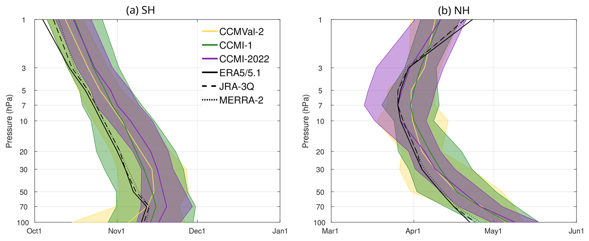
Figure 13Descent of the final warming date in the SH (a) and the NH (b), computed as the day when the zonal-mean zonal wind at 60° latitude crosses the 30 m s−1 line in the SH, and the 5 m s−1 line in the NH. Based on monthly mean output interpolated to daily values for the period 1980–2000.
It is evident that in all model generations, the vortex breakdown occurs too late in both hemispheres, and this delay is larger in the SH. In the newest generation, the FWD bias is even more pronounced, being up to 3 weeks for the MMMed in the SH lower stratosphere and up to 1 month considering the intermodel spread. For instance, at 50 hPa, the reanalyses place the FWD at the beginning of November, and CCMI-2022 places it almost at the end of the month. In the NH, the late bias is more modest (∼ 1–2 weeks), and similar in the three generations, with reanalyses placing the FWD at 50 hPa in mid-April (with larger interannual variability than in the SH, not shown) and models at the end of April-beginning of May. It is noticeable that the bias extends throughout the stratosphere, and in the NH it reverses sign in the upper stratosphere.
In summary, the models have too weak downwelling, especially in SH spring (September–October). On average the models tend to underestimate the peak in resolved wave activity entering the stratosphere, and have difficulties in capturing its timing in the SH. In addition, the polar vortex lasts too long, especially in the SH, in all model generations, which results in too large downwelling in December.
3.5 Ozone
After discussing the main transport processes, we turn to the representation of the stratospheric ozone climatology, as capturing the evolution of the ozone layer is one of the key motivations for the development of CCMs. We examine partial ozone columns (in Dobson Units, DU) computed from the models' output volume mixing ratios (in mol mol−1) over two vertical layers: the lower stratosphere, computed between 100–20 hPa in the tropics and between 150–20 hPa in the extratropics, and the upper stratosphere, computed over 10–1 hPa. Because ozone is an output available for all the models, we included only the common models, which are the 8 model families introduced in Tables 1–3 (the corresponding figures for all models are shown in the Supplement, Figs. S26 and S27).
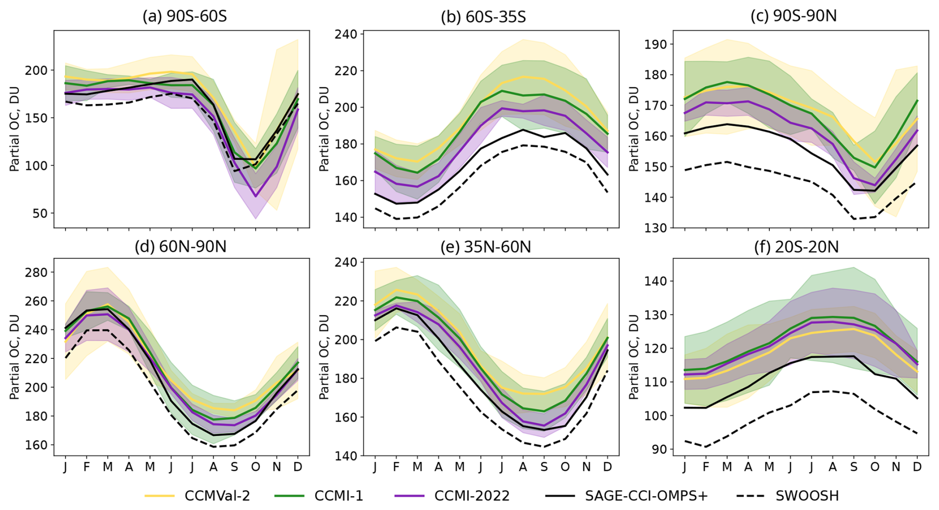
Figure 14Seasonal cycle of lower stratospheric ozone column averaged over different latitudinal regions (note the different scale in each panel). The column is defined as 100–20 hPa in the tropics and 150–20 hPa in the extratropics. Only common models are included in this figure (F1–F8 defined in Tables 1–3). The corresponding figure version showing all models across the three generations is in the Supplementary material. Period: 1990–2010 (1980–2000 for CCMVal-2).
The two satellite datasets show some differences, with generally lower ozone values for SWOOSH when compared to SAGE-CCI-OMPS+ (∼ 10–15 DU). This observational uncertainty is consistent with the typical uncertainty for satellite data at these altitudes (e.g. Hubert et al., 2016). Overall, all model generations overestimate ozone in the lower stratosphere, especially in the SH midlatitudes and in the tropics (Fig. 14b, f), which results in a globally integrated (90° S–90° N) lower stratospheric ozone bias of about ∼ 15 DU (Fig. 14c). In contrast to previous generations, the latest generation (CCMI-2022) overestimates SH polar ozone decline in October–November by about 25 DU (∼ 25 %; Fig. 14a), also when considering all the models (Supplement Figs. S29 and S31). Both the depth and duration of ozone decline are overestimated in CCMI-2022, with the observations falling on the high end of the inter-model spread. The large ozone decline in the latest generation is likely related to the particularly large delay in the vortex breakdown date (Fig. 13a). A long-lived polar vortex can imply maintained low polar cap temperatures that facilitate heterogeneous chemical ozone destruction. Moreover, the low ozone could be in turn contributing to the cold pole bias, since the low ozone mixing ratios absorb less solar radiation, resulting in a colder polar stratosphere, which induces a stronger polar vortex to maintain thermal wind balance.
Despite the mean biases, the models are generally able to correctly capture the lower stratospheric ozone seasonality, with correlations between the observational and model seasonal cycles above 0.95 (see Taylor diagrams in Supplement Figs. S31–S35). The lowest correlations (less accurate representations of the seasonality) are found in the SH polar region.
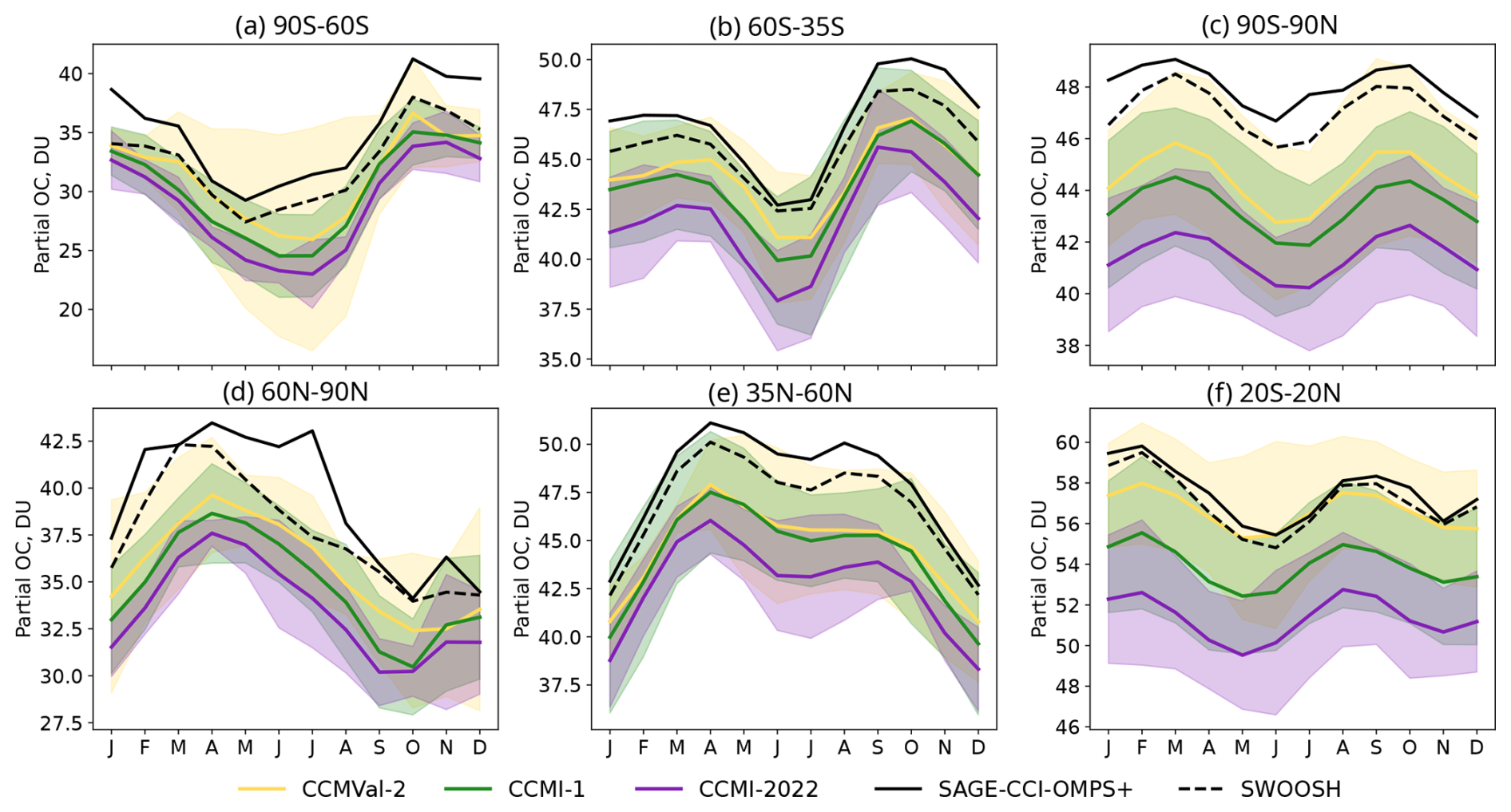
In contrast with the lower stratosphere, ozone in the upper stratosphere is underestimated by the models in the global mean (about ∼ 10 %; Fig. 15c). The underestimation is found in all regions, and is most severe in the newest generation (CCMI-2022), also when considering only common models (Supplement Fig. S30). The reason for the opposite model biases in the global lower and upper stratosphere is unclear. The seasonality is reasonably captured in general (correlation above 0.9, see Taylor diagrams in Supplement Figs. S36–S40), with highest correlations found in midlatitudes, and the lowest correlations in the polar regions. Note that the agreement between the datasets is also weakest in the polar caps, possibly due to sparser coverage of these regions.
3.5.1 Cly and release fraction
Another crucial factor for stratospheric ozone loss, in addition to the dynamical conditions, is the amount of active chlorine present in the lower stratosphere. The chlorinated long-lived source gas species emitted at the surface (e.g. chlorofluorocarbons, CFCs) are decomposed in the stratosphere by photolysis, reaction with O(1D) and reaction with OH to form inorganic chlorine (Cly). Cly comprises reservoir species (such as HCl) and ozone-destroying active chlorine (e.g. ClO). Conversion of the source gases occurs as air masses are transported from the tropical tropopause to the polar stratosphere by the stratospheric circulation. The photolysis (and other oxidation) rates are a function of latitude and altitude, as they depend on the exposure of air parcels to solar radiation. Thus, the fraction of a long-lived source gas in an air mass that has been converted depends on the specific transport pathway followed. It is important to note that the photolysis rates are not identical in the models being studied, and thus we cannot completely disentangle transport from chemistry. Nevertheless, if we assume that the differences in photolysis rates across the models are smaller than those in transport, then the differences between the amounts of Cly in a given region reflect primarily differences in the transport of air parcels across the stratosphere.
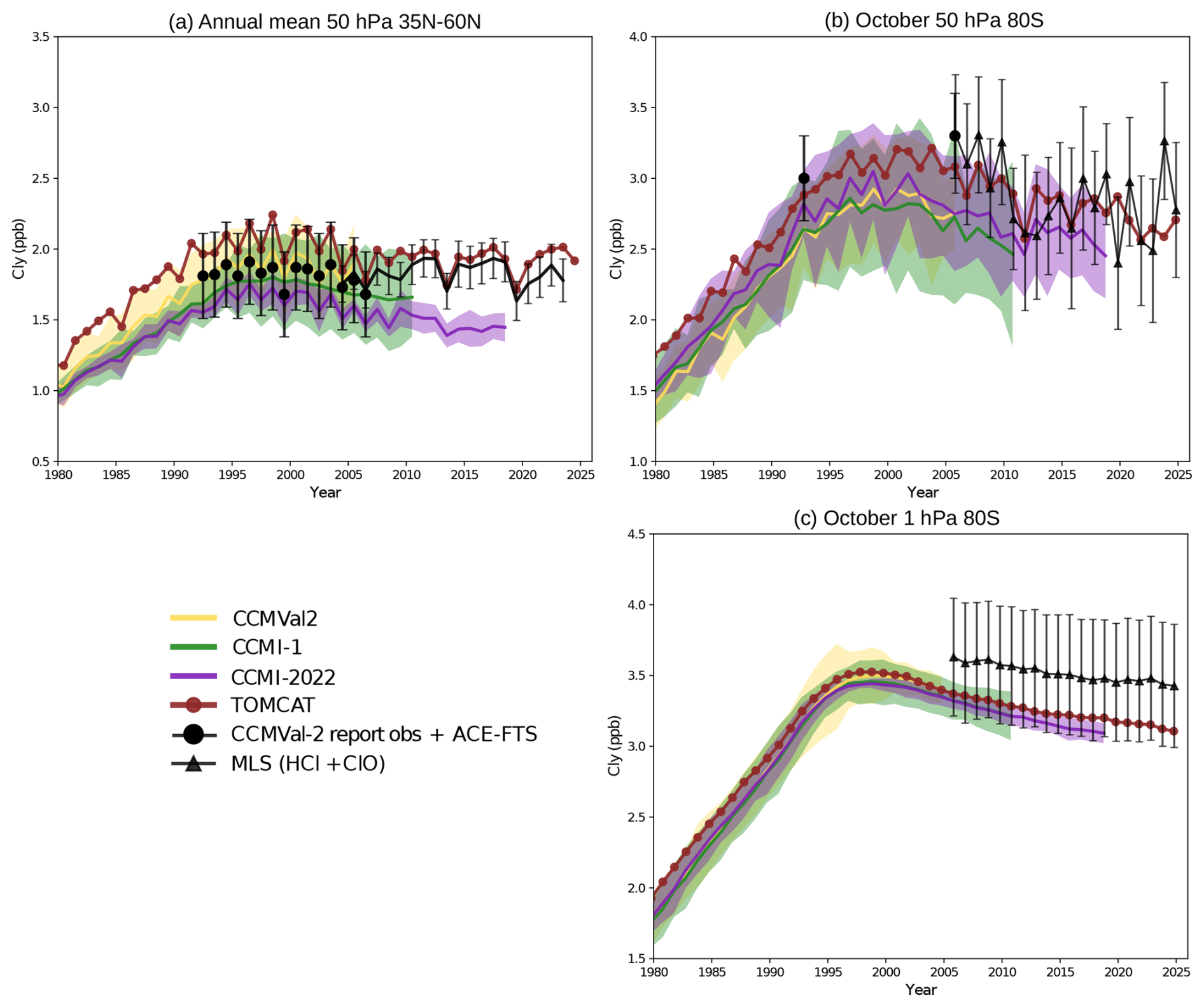
Figure 16Observed (black lines and symbols) and modelled Cly timeseries between 1980 and 2025 for the multi-model median and its associated envelope of uncertainty (MAD) in the three model generations and TOMCAT CTM simulation. (a) Annual-mean NH mid-latitude (35–60° N) at 50 hPa. (b) 80° S, Antarctic spring (October) at 50 hPa. (c) 80° S, Antarctic spring (October) at 1hPa. Note that the MMMed contains a different number of models for each generation of CCMs. The observations shown are taken from different instruments; in panel (a), the values until 2006 are taken from the CCMVal-2 report and beyond 2006 are from ACE-FTS Cly (HClClO+HOCl); in panel (b), the 1992 value is from UARS HALOE HCl, the 2005 value from Aura MLS HCl and beyond that from Aura MLS (HCl+ClO). The latter observations are shown also in panel (c). Vertical error bars in the observations denote the standard deviations of the measurements.
The models capture the overall trend of the evolution of Cly as simulated by TOMCAT, with similar increasing slopes peaking in the late 1990s, followed by a slower decline. In the NH midlatitudes (Fig. 16a), during the 1990s and early 2000s, the TOMCAT values are higher than the available observations, although they are within the uncertainty range. Also, this can be explained by the HALOE and Aura-MLS observational estimates (in this panel only) missing the ClONO2 component of Cly, which makes up between 5 and 10 % (thus around 0.2 pptv) of the total Cly. After 2005, there is a very good agreement between TOMCAT and ACE-FTS (which indeed comprises the main components of Cly). The oldest generation (CCMVal-2) agrees well with the observations and slightly underestimates the TOMCAT 3-D CTM, while CCMI-1 and even more so CCMI-2022 underestimate the Cly values in the NH midlatitudes, especially after 2005 when the Cly measure becomes more complete and ACE-FTS and TOMCAT agree well with each other. This could be reflecting the particularly large young bias in the mean age of air in CCMI-2022 (Sect. 3.1), as the air parcels reaching the 50 hPa level have less time to photolyze the source gases as they are transported too fast through the stratosphere. In the SH polar lower stratosphere (Fig. 16b), there are only two observational points before 2005, which show reasonable agreement with TOMCAT, considering the error bars. After 2005, MLS shows reasonable agreement with TOMCAT, except for the last few years, when TOMCAT suggests a faster decline in Cly than MLS. In this region, there is no clear difference among model generations, and all show an underestimation of Cly, although there is a very large spread that includes the observational estimates.
Figure 16c shows timeseries of Cly at 1 hPa, which provides a verification for the maximum Cly in a model. At this altitude, the vast majority of Cl-containing organic source gases have undergone complete photolysis. At this level, Cly should not be more than the total Cl at the surface, taking account of a lag due to transport timescales. This is well satisfied by the MMMed and MAD spread for the three generations, although not for some individual models, as seen in Fig. S41 of the Supplement. These outliers have been removed to compile Fig. 16. Nevertheless, we emphasize the need to examine the Cly timeseries when analyzing ozone recovery in individual models. Simulation of realistic stratospheric Cly, based on specified surface ODS time series, should be a pre-requisite for quantifying the impact of ODSs on stratospheric ozone. The outliers in Fig. S41 appear to strongly deviate from expectations in this regard.
A complementary diagnostic is to represent the PDF of the fractional release for a given CFC against the corresponding mean age of the same air parcel (Schauffler et al., 2003; Douglass et al., 2008; Engel et al., 2018). Fractional release is the fraction of a long-lived source gas that has been destroyed (by photolysis or other reactions) since entering the stratosphere. It is calculated as the stratospheric mixing ratio of the CFC in an air parcel (χ) and the mixing ratio in the same air parcel when it entered the stratosphere (χentry) using the following equation: . Given the dependence of photolysis rates with altitude mentioned above, an air parcel of a certain age will have a larger fractional release if it travelled higher in the stratosphere than if it had a lower-altitude pathway.
Fractional release in the models is compared with that calculated based on the new global age of air climatology from ACE-FTS (Garny et al., 2024b; Saunders et al., 2025). This is a vast improvement over the 5 data points that were available for the SPARC (2010) report. For ACE-FTS, a fractional release value could be calculated for each bin (1 month, 10°, 3 km) using the mean age of air and the mean CFC-12 concentration. NOAA Marine Boundary Layer surface measurements were used as a reference to determine the observational mixing ratio upon entry into the stratosphere (Saunders et al., 2025). As such, the CFC-12 measurements are bias-corrected using the reference curve to also account for transit time to the tropopause.
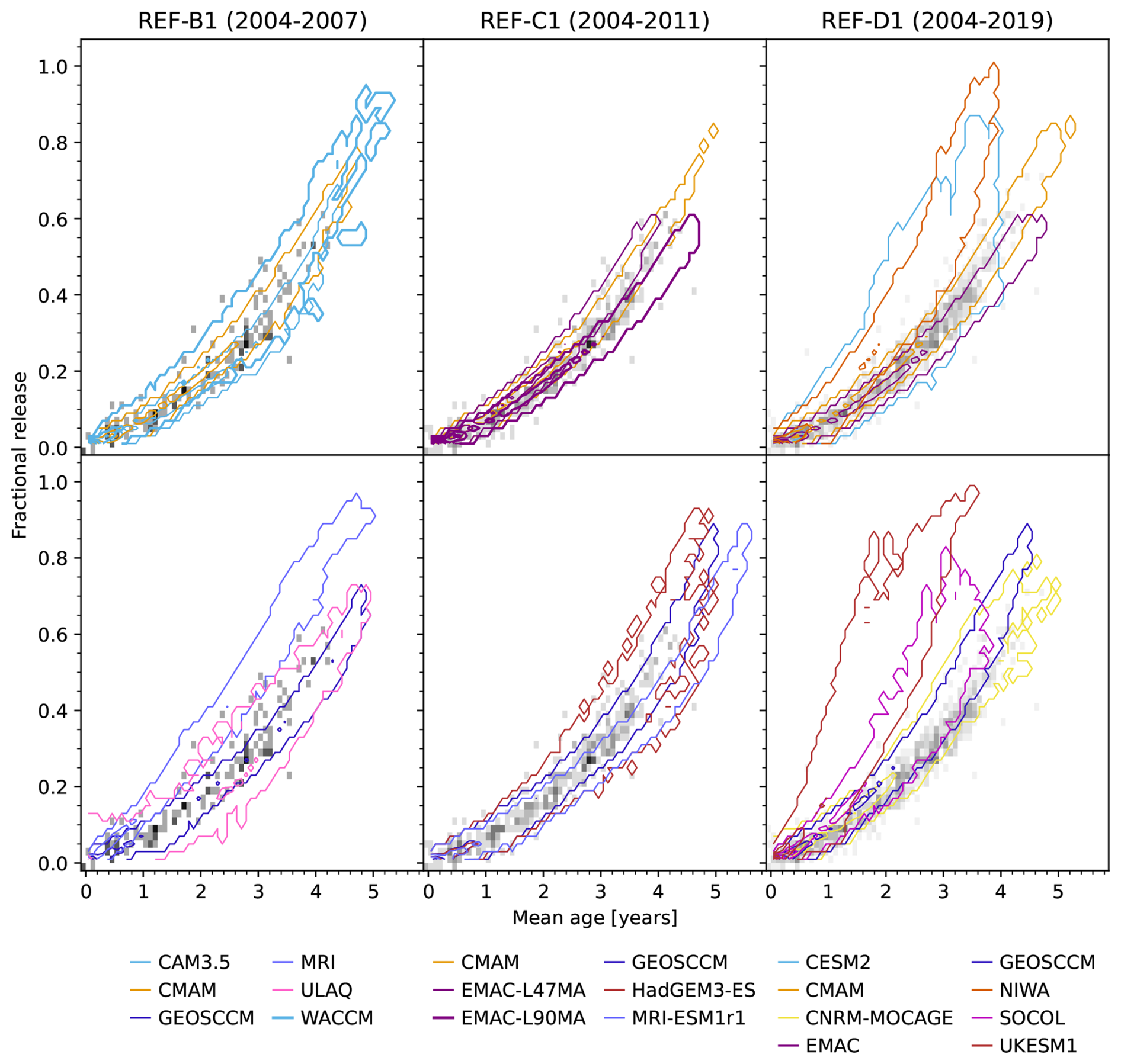
Figure 17Probability density function of fractional release as a function of mean age of air computed for CFC-12 in observations and models. Unitless (counts normalized by total number of counts). Contours range up to to 0.06 spaced by 0.01. Gray shading shows the observational results (see text for description of observations used, darker gray corresponds to normalized count of 0.025). Only northern hemispheric points from 50–100 hPa for the time period indicated are included (using 2004–2007 for all generations does not change the results qualitatively). The models are split across two vertical panels for each model generation for easier interpretation of the results. Mean age for the models is relative to its 100 hPa value.
Overall, the results in Fig. 17 show that the agreement for fractional release with the observations is best for CCMI-1 models, and that in CCMI-2022, most models have too much fractional release for a given mean age value. If we again assume that the photolysis rates are not too different across the models, this implies that the models are transporting air masses too fast into the higher levels, where they photolyze more efficiently. Analogously, a given photolysis rate is obtained at too low mean age values in the models, indicating that air reaching up to a given level (where photolysis is efficient) is too young.
We note that Figs. 16 and 17 can seem to provide inconsistent information. Figure 16 suggests that photolysis in CCMI-2022 is too small for a given pressure level in the stratosphere, while Fig. 17 shows that fractional release is too high in CCMI-2022 for a given mean age value. However, due to the young age bias in CCMI-2022 (Fig. 1), a given mean age value corresponds to a higher pressure level in the models than in the observations. Hence, looking at mean age space yields different results than looking at altitude/pressure space. Consider, for example, an air parcel that is 4 years old and resides at 50 hPa in the NH midlatitudes. In the observations, it has undergone a given amount of fractional release. In the CCMI-2022 models, a similar 4 year-old air parcel has undergone a larger amount of fractional release (possibly due to spending too much time at high altitudes). However, because the transport is too fast in the models, that 4 year-old air parcel is located too high in the stratosphere, while the parcel at 50 hPa has a younger mean age, and thus has had less time to produce Cly.
We recall that the different mean age values do not reflect differences in the residual circulation, but mostly in mixing efficiency (Fig. 2). This could imply that air parcels of a given mean age in models spent too much time mixing and recirculating at high altitudes, where photolysis is more efficient. However, without knowing the shape of the age spectrum, it is not possible to reach further conclusions on the reason for the high fractional release for a given mean age value. It is also possible that the low Cly values are partly due to too weak polar downwelling in SH spring, which brings down Cly produced at higher levels. Finally, we note that differences between ODS scenarios used in the successive model generations are relatively small and will not affect the results substantially (Lickley et al., 2024).
In summary, the ozone is overestimated by the models in the lower stratosphere tropics and SH midlatitudes and generally underestimated in the upper stratosphere. The polar ozone loss in SH spring is overestimated in the newest model generation. However, the Cly values are too small compared to observations, probably due to the too fast transport and/or to the underestimated downward mass flux in SH spring. This points to the cause of excessive ozone loss in October being the too strong polar vortex, and not the availability of active chlorine.
In this section, we address the changes over the past 4 decades. We focus on the common period for the three model generations within the satellite era (1980–2000), and examine the difference pre and post year 2000 only for the newest generation (CCMI-2022).
4.1 Changes in mean age of air
Figure 18a shows the 1980–1999 trends for the three model generations in global mean AoA. There is a good intergenerational agreement in the MMMed, with negative trends peaking in the lower stratosphere at around −6 % per decade. At higher levels, the newer generations show −5 % and −4 % per decade for CCMI-2022 and CCMI-1, nearly constant with height, and linearly decreasing to −3.5 % per decade for CCMVal-2. There is considerably large spread, especially in the older generations, and surprisingly reduced in the newest one for the lower stratosphere.
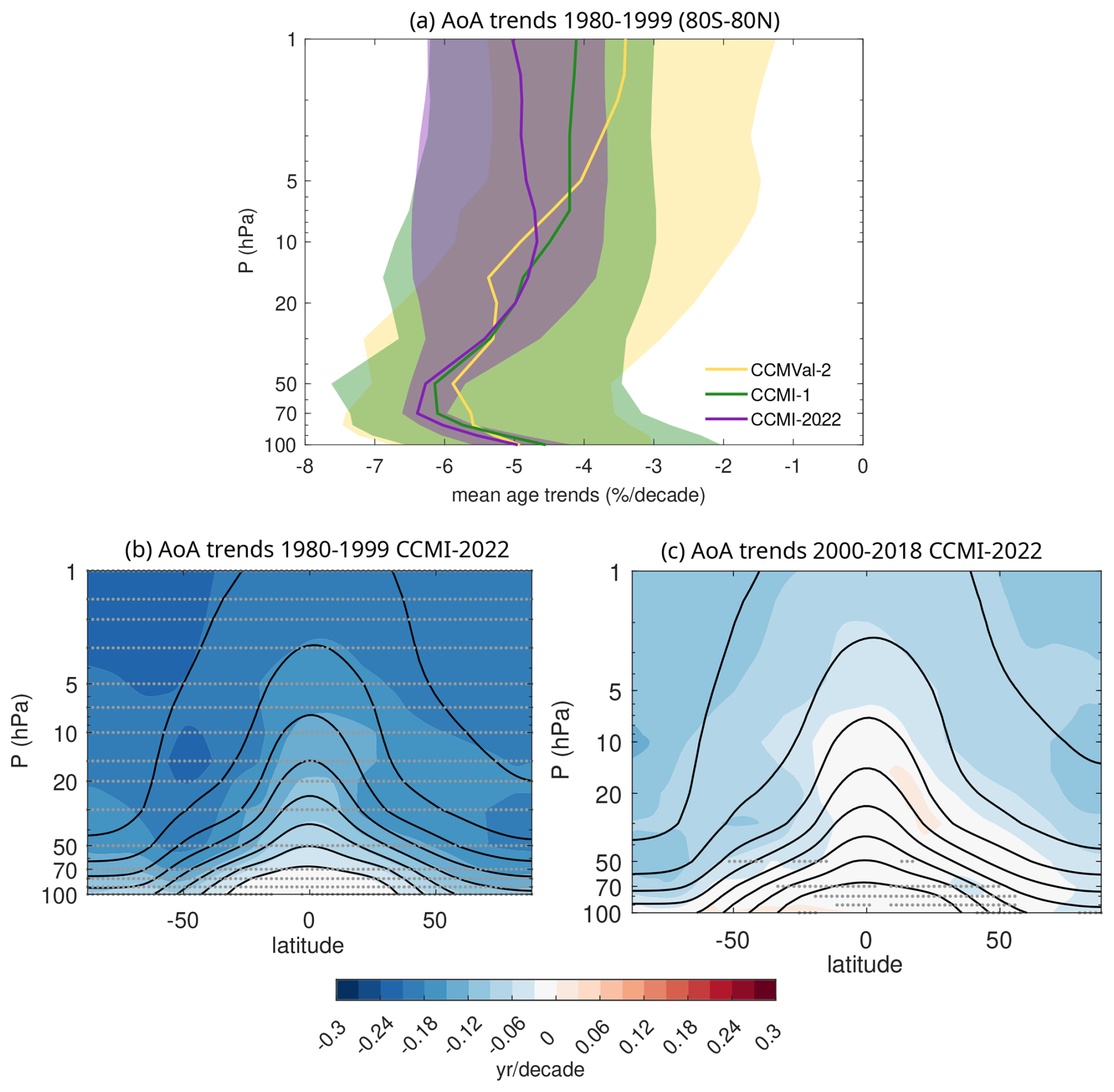
Figure 18(a) Trends in mean age of air for the three generations over the period 1980–1999 (lines show the MMMed and shading the 15th to 85th percentile range). (b, c) cross section of mean age of air trends for the CCMI-2022 MMMed for the ozone depletion (b) and recovery (c) periods. In (b) and (c) the trends are computed after regressing out the natural variability (ENSO, QBO, solar cycle and aerosols; see text for details). Stippling indicates where all the models agree in the sign of the trends.
Previous studies have shown that SH ozone depletion has contributed significantly to enhancing the BDC trends over the last two decades of the 20th century (e.g., Oman et al., 2009; Oberländer et al., 2013; McLandress et al., 2010; Polvani et al., 2018). This is due to the acceleration of the residual circulation forced by the dynamical effects of ozone depletion in the SH polar lower stratosphere (McLandress et al., 2010; Abalos et al., 2019). In order to explore this effect, Fig. 18b and c show the AoA trends in CCMI-2022 over the ODS increase period (1980–1999) and the ODS decline period (2000–2018), which we refer to as ozone depletion and recovery periods, respectively. In order to remove the effect of natural variability on these short-term trends, we have applied a multiple linear regression to the CCMI-2022 AoA using as regressors the Multivariate ENSO Index Version 2 (https://www.psl.noaa.gov/enso/mei, last access: 18 April 2026), two QBO indices corresponding to the two principal components of the equatorial mean wind between 70 and 10 hPa (Wallace et al., 1993), the solar 10.7 flux (https://psl.noaa.gov/data/correlation/solar.data, last access: 18 April 2026), and the Global Space-based Stratospheric Aerosol Climatology Version 2.0 (GloSSAC, 2018). We apply the regression to the newest generation over the period 1980–2018 and compute the trends for the residuals over the shorter periods. The results are qualitatively consistent with those obtained with the full field, in particular the 1980–1999 trends remain practically unchanged (Fig. S43 of Supplement). Consistent with previous literature, the mean age trends are substantially reduced in the latter period compared to the former. The change in the global mean AoA trend from the first to the second period is even larger than found before for longer periods (from 6 % per decade to 1 % per decade). In addition, the trends are much more robust in the first period, with all models presenting negative trends (Supplement, Fig. S42). An additional proof that the Antarctic ozone hole is behind the large trend before 2000 is that the negative AoA trends are larger in the SH hemisphere over the earlier period. This is consistently seen in the three generations (Fig. S44 of Supplement). In the post-2000 period the much smaller trends still display an asymmetry, being more negative in the SH than in the NH, consistent with previous studies (e.g., Ploeger and Garny, 2022).
4.2 Changes in advection by the mean meridional overturning circulation
Figure 19a–c shows the trends of the annual mean upward (Fig. 19b) and downward (Fig. 19a, c) net mass flux of the residual circulation for the three generations and three reanalyses. Again, there is a very good quantitative agreement across generations for the MMMed trends, with a spread that increases with altitude and is reduced in the newest generation. The upward mass flux accelerates 1 %–2 % per decade over the lower and middle stratosphere (below ∼ 5 hPa), and the trends are much reduced and uncertain in the upper stratosphere, although positive for the MMMed in the three generations. Both hemispheres show strengthened downwelling in the lower and middle stratosphere, and the trends are larger and more significant in the SH, especially between ∼ 50 and 10 hPa. At higher levels, there is a larger spread across the model generations and within each generation. The reanalyses show very diverse results. The upward mass flux increases significantly by 4 %–6 % per decade in the lower stratosphere according to MERRA-2 and JRA-3Q, while it decreases up to −2 % per decade in this region in ERA5. This reanalysis discrepancy is consistent with Šácha et al. (2024). The downwelling trends also differ significantly across reanalyses. In the SH, the three reanalyses indicate an acceleration (albeit with very different magnitudes), while in the NH, even the sign is different across the reanalyses.
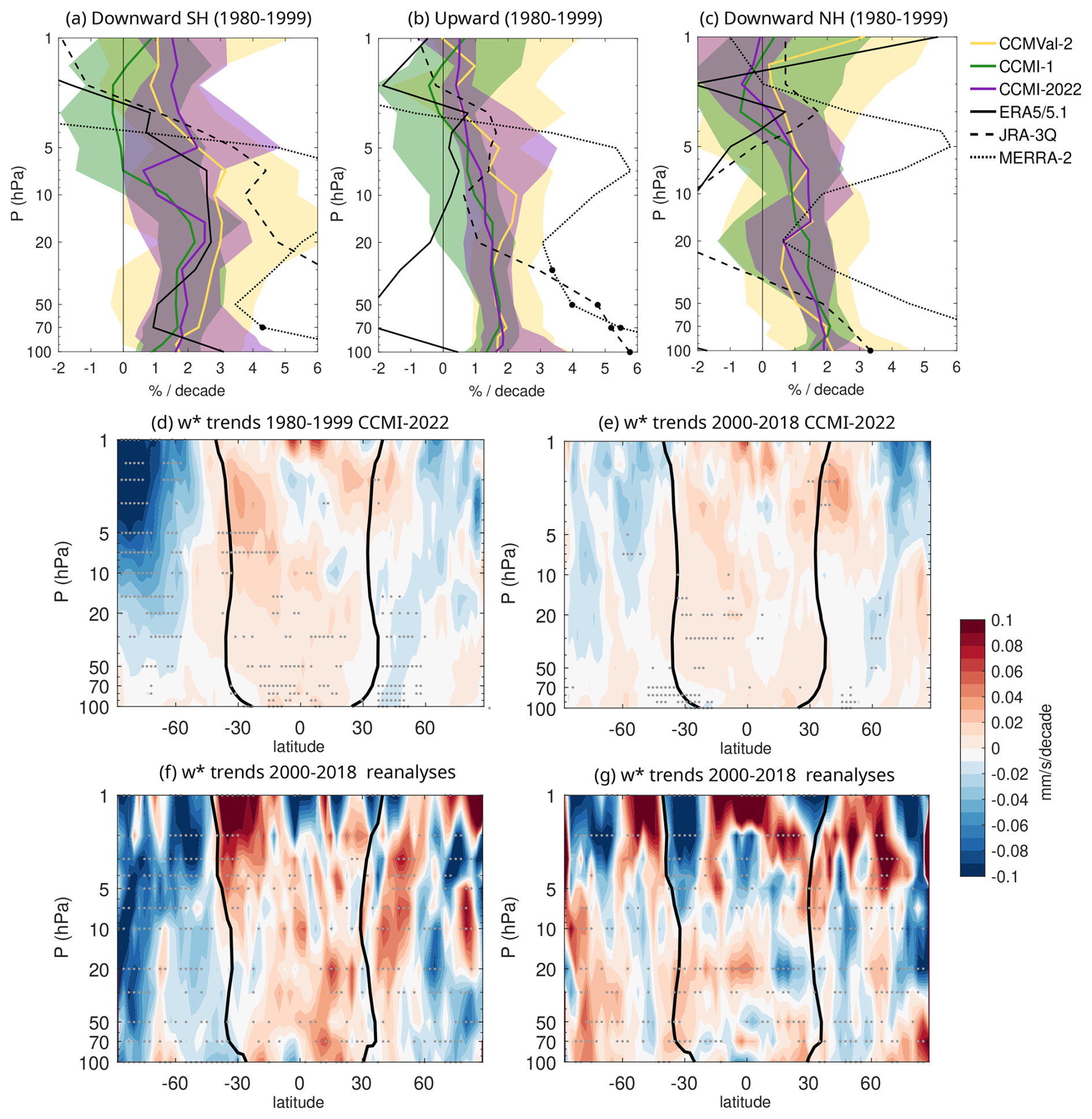
Figure 19(a–c) Trends of upward mass flux (b) and downward mass flux in the SH (a) and NH (c) over 1980–1999 in the 3 generations of models and reanalyses. The only statistically significant trends in the reanalyses are those marked with a closed circle, based on a Student's t test with a 95 % confidence level. (d, e) Cross-sections of the vertical component of the residual circulation trends for the CCMI-2022 MMMed for the ozone depletion (d) and recovery (e) periods. (f, g) Same as (d), (e) but for the multi-reanalysis mean (MRM). In (d)–(g) the trends are computed after regressing out the natural variability (ENSO, QBO, solar cycle and aerosols; see text for details). Black contours show the MMMed (d, e) and the MRM (f, g) turnaround latitudes. Stippling indicates where all the models (d, e) or all the reanalyses (f, g) agree in the sign of the trends.
Figure 19d, e shows the trends of the vertical component of the residual circulation for the periods before and after 2000 in the CCMI-2022 simulations' multi-model median. The model results show an acceleration of tropical upwelling and extratropical downwelling during both periods, with considerably larger SH downwelling acceleration in the first period. While there is no attribution made in this analysis, these results are in line with the large impact of ozone depletion on the acceleration of the residual circulation found in previous studies. Figure 19f, g shows the average of the trends for the three reanalyses. The averaged reanalysis trends are noisier than the model trends, but display an overall consistent behavior, with larger tropical upwelling and polar downwelling in the SH in the ozone depletion period. Again, the results are highly consistent when no variability is removed (Fig. S46 of the Supplement).
One of the most robust atmospheric responses to increasing greenhouse gases is a rise in tropopause height, resulting from the combined effects of tropospheric warming and stratospheric cooling, which jointly shift the lapse-rate boundary between the two layers upward. This is captured by all models, as seen in the timeseries in Fig. 20a. The rise of the tropopause is similar in the three model generations (∼ −0.5 hPa per decade over 1980–2010), consistent with the value given by Gettelman et al. (2010) for CCMVal-2 models, and slightly lower than that in the three reanalyses (∼ −1 hPa per decade).
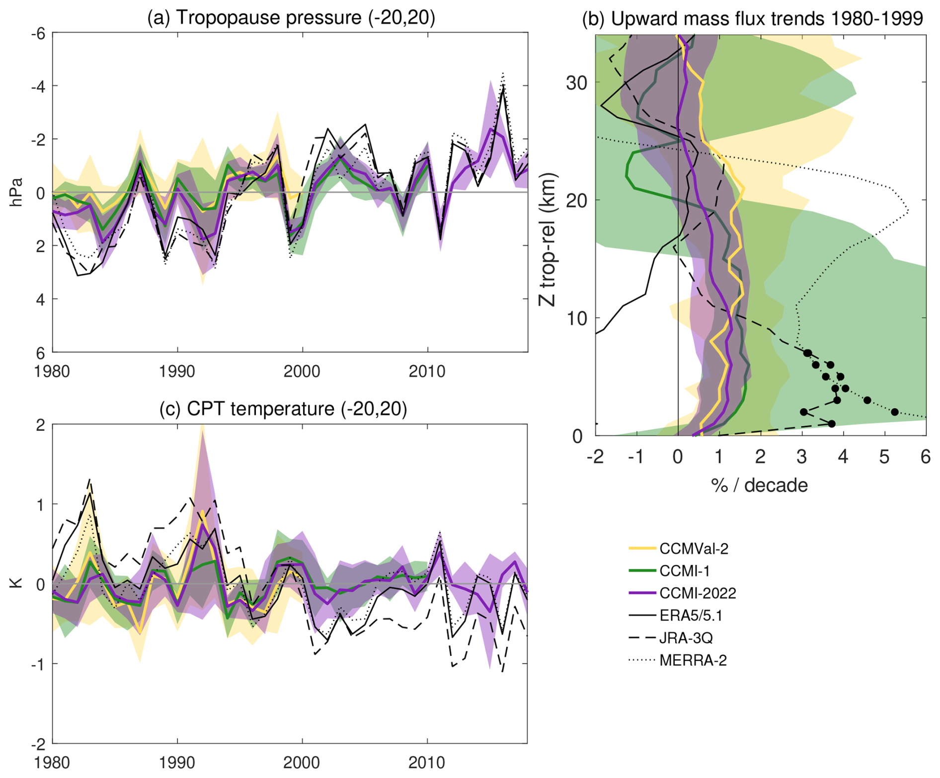
Figure 20(a) Timeseries of CPT pressure (1980–2018). (b) Tropopause-relative trends of upward mass flux over 1980–1999. (c) Time series of CPT temperature (1980–2019).
Previous studies have shown that tropical upwelling trends are significantly different when viewed from a tropopause-relative coordinate (Oberländer-Hayn et al., 2016). Figure 20b shows the trends of the upward mass flux over 1980–1999 (similar to Fig. 19b) in tropopause-relative coordinates. This is computed by regridding the mass flux timeseries at each level into a tropopause-relative log-pressure altitude grid (using the tropopause pressure averaged over 20° S–20° N) and then computing the trends. It is clear that the trends decrease substantially at the tropopause level, where the models simulate near-zero trends in tropopause-relative coordinates, and ∼ 1 %–2 % per decade on pressure coordinates. On the other hand, at higher levels, the trends are only slightly lower than those in Fig. 19b (trend values differ less than 0.5 % per decade). In any case, we note that both the decrease in tropopause pressure and the acceleration of tropical upwelling largely arise from the same primary underlying driver, namely tropospheric warming. Therefore, the rising tropopause should not be considered a cause of tropical upwelling acceleration, but rather both are a common response.
Coupled radiative-dynamical responses to climate-forcing affect tropopause temperature, which in turn determine the transport of water vapor into the stratosphere. Figure 20c shows that the cold point tropopause is cooling in the three reanalyses between 1980 and 2010 (around −0.29 ± 0.14, −0.54 ± 0.16, and −0.13 ± 0.15 K per decade in ERA5/5.1, JRA-3Q and MERRA-2, respectively). On the other hand, the CCM multi-model medians of the three generations show a near-zero trend over this period (0.040 ± 0.25, 0.060 ± 0.082 and 0.035 ± 0.098 K per decade for CCMIVal2 – until 2000 –, CCMI-1 and CCMI-2022, respectively). The trend in the reanalyses is partially explained by a strong drop in cold point temperature after the year 2000, which was a random feature not necessarily to be expected in the model simulations, but which exacerbates the underlying negative trend. Note that future climate simulations project a cold point warming (Gettelman et al., 2010), and a warming has been detected in observations since 2000 (Zolghadrshojaee et al., 2024).
4.3 Changes in mixing
Changes in AoA are not only related to changes of advective transport by the residual circulation, but also to mixing efficiency (Eichinger et al., 2019). Eichinger et al. (2019) show that the contribution of changes in mixing efficiency to the future changes in AoA in CCMI-1 refC2 simulations present a large spread across models, varying between 10 % and 30 %. Moreover, consistent with the results for the climatology obtained by Dietmüller et al. (2018) and captured here in Fig. 2, they show that the spread in mixing efficiency changes is closely correlated with the spread in the magnitude of the AoA decrease over the 21st century. To test this behavior, Fig. 21 shows the scatter plot of changes between the two decades centered in 1980 and 1999 (1975–1984 and 1994–2003) in mean age versus RCTT and mixing efficiency.
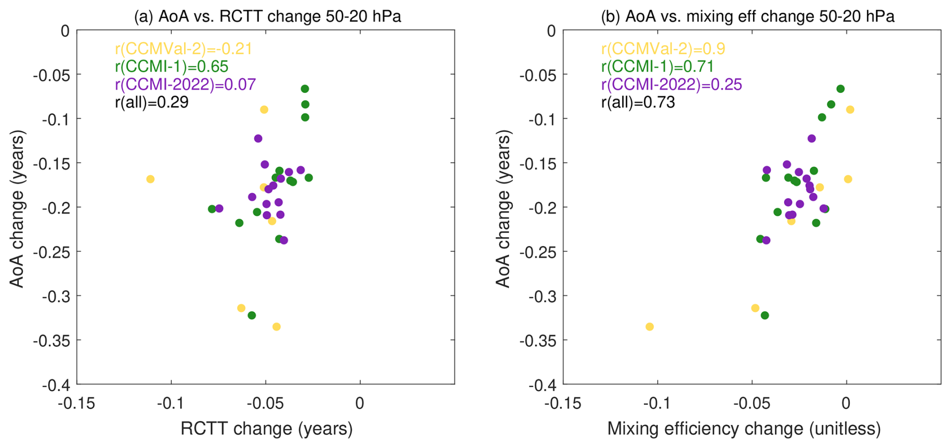
Figure 21Scatter plots of changes between 1975–1984 and 1994–2003 in AoA versus RCTT (a) and AoA versus mixing efficiency (b).
The results show overall higher correlations of the changes in mean age with changes in mixing efficiency than with changes in RCTT, consistent with the results for future climate simulations described above. However, this result is less robust than for the climatology (Fig. 2), because for CCMI-1 the correlation between mean age and RCTT is notably higher than for the other generations. Also, the correlation with mixing efficiency is low in CCMI-2022 (0.25). Nevertheless, for any given generation (including CCMI-1), and for all generations together, the correlations are higher with mixing efficiency than with RCTT. This suggests that the mean age changes are more strongly connected with changes in mixing or diffusion than with the changing strength of the residual circulation.
4.4 Changes in polar processes
Ozone depletion over Antarctica has impacted not only the strength of the residual circulation but also the polar vortex. Specifically, it is known that ozone depletion cooled the polar lower stratosphere in SH spring and strengthened the polar vortex, leading to a delay of the final warming date. Figure 22 shows the trends of the FWD over the period 1980–1999 for the SH polar vortex, computed as the day when the zonal-mean zonal wind reaches a value of 30 m s−1 at 50 hPa.
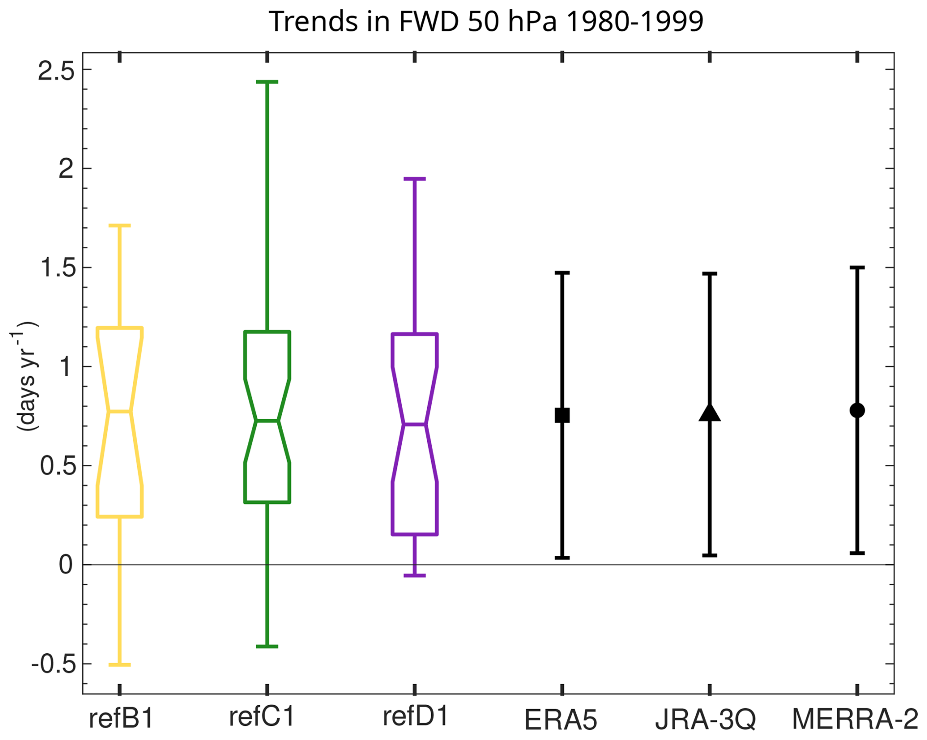
Figure 22Trends of FWD in the SH over the period 1980–1999. The horizontal lines in the boxes show the MMMed, the height of the boxes represents the interquartile (25th–75th percentile) range, and the whiskers extend from the minimum to the maximum values. The error bars for the reanalyses show the 95 % confidence interval based on a Student's t-test distribution for the linear trend.
The reanalyses show a FWD delay of ∼ 8 d per decade, with very good agreement across them and large error bars due to the large interannual variability. The MMMed of the three generations captures this trend very well. Nevertheless, there is a very large spread across the individual models, with some models even producing negative trends. The newest generation performs best in capturing these trends: although it exhibits the largest interquartile range, it produces fewer extreme values, and almost all models show a positive trend.
4.5 Ozone changes
We lastly examine the temporal evolution of the ozone columns analyzed in Sect. 3.5.
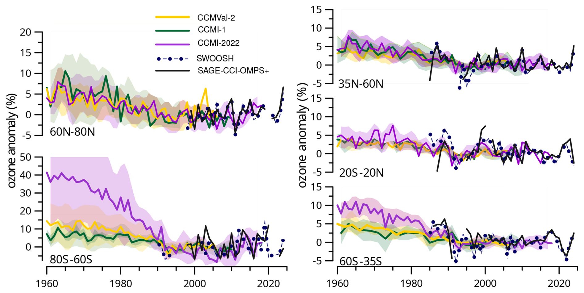
Figure 23Evolution of annual mean O3 partial column anomalies in the lower stratosphere (100–20 hPa in the tropics, 150–20 hPa in the extratropics) from the three generations of models compared to SWOOSH and SAGE-CCI-OMPS+ satellite data. Only common models are included, as identified in Tables 1–3. Anomalies are computed with respect to the base period 2000–2010 (except CCMVal-2, which uses 1990–2000). Observations are not included in the polar regions because there are very few points before 2005.
Figure 23 shows the annual mean ozone anomalies evolution in the lower stratosphere from the three generations of models compared to the SWOOSH and SAGE-CCI-OMPS+ datasets. All three model generations simulate a steady decline of lower-stratospheric ozone from 1960 to the end of the 1990s, with close agreement among models except for the SH polar latitude band (85–60° S), where CCMI-2022 shows a notably larger decline. This difference could be partly due to updated ODS and GHG forcings. However, these are not very different over the historical period (Lickley et al., 2024), and thus it is likely that the newer models are more sensitive to the external forcings. The larger decline in the SH is consistent with the lower climatologically averaged ozone in Fig. 14a in October and November, which is in turn related to the longer-lasting polar vortex in this generation (Fig. 13a). Note that the faster decline in CCMI-2022 is partly driven by the UKESM-StratTrop model (see Supplement Fig. S47), which presents ozone anomalies of 60 up to over 100 DU in the 1960s to 1980s. This model indeed severely overestimates ozone decline (by ∼ 40 DU, see Supplement Fig. S31). However, the other models also show larger ozone column anomalies compared to the previous generations, with most models starting above 20 DU in 1960, while staying below that value in previous generations.
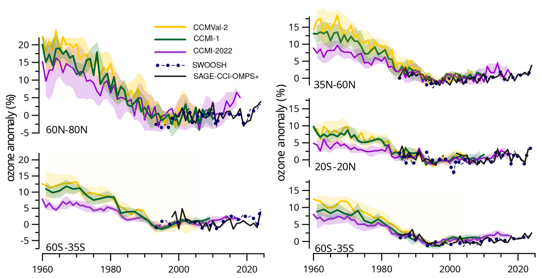
The equivalent plot for the upper stratosphere is shown in Fig. 24. Both satellite and models show a sharp decline from the 1960s up to the end of the 1990s, followed by slightly upward trends, consistent with the statistically significant ozone recovery detected in the upper stratosphere (e.g. WMO, 2022). There is a general agreement across model generations over the satellite era (after 1985). Before then, the depletion is slightly stronger for the oldest generation than the following ones. There is close agreement between the models and the satellite records, with smaller interannual variability than in the lower stratosphere.
In this study, we evaluate several aspects of stratospheric transport and dynamics relevant for the representation of the stratospheric ozone layer in models participating in three most recent CCM intercomparison initiatives, which we denote model generations (CCMVal2, CCMI-1 and CCMI-2022), using the historical simulations (refB1, refC1 and refD1, respectively). Inspired by the SPARC (2010) report and subsequent literature, we select a subset of key diagnostics to evaluate the model results against modern observational (satellite) and reanalysis datasets. Different from the SPARC report, the focus here is not to identify and understand issues in every individual model, but rather to examine the evolution across three CCM generations over the last 15 years, and to provide an assessment of the outstanding weaknesses and strengths in the representation of stratospheric transport. We focus on the climatology and also examine the past trends, which are to a large extent associated with dynamical effects of ozone depletion over the last two decades of the 20th century.
Overall, we find little progress in the representation of key transport processes, and several longstanding biases persist or are even worse, on average, in the newest models (CCMI-2022). In particular, the young bias in mean age of air and the late breakdown of the SH polar vortex are more pronounced in the most recent generation. The ozone concentrations in the SH polar lower stratosphere in spring are biased low in CCMI-2022, while they were in good agreement with observations in the previous generations.
The simulated stratospheric mean age of air is on average too young in the three model generations, especially in the middle to upper stratosphere and at high latitudes. This bias is about one year for the global average between 100 and 15 hPa in the CCMI-2022 multi-model median. This implies that stratospheric transport is too fast. The mean meridional overturning circulation is slightly overestimated (by ∼ 10 %) in the models' lower stratosphere (especially in CCMI-2022), which is qualitatively consistent with a younger mean age. However, the mean age bias is most likely also related to mixing and diffusion effects. Indeed, a large fraction of the spread in mean age of air across the models is correlated with the spread in mixing efficiency in the three model generations, consistent with previous studies. While there is also some evidence pointing to slightly too weak mixing between tropics and extratropics, this is not supported by the N2O structure and could instead reflect excessive vertical diffusion in the tropical stratosphere or other biases. These factors could contribute to explain young bias on average. Nevertheless, note that the age bias could have different origins in the various models. For instance, a recent study relates the young bias in the newest generation of the GEOSCCM model compared to its predecessors to a bias in tropical upwelling arising from differences in the transport scheme (Orbe et al., 2025).
In the polar stratosphere, we find an underestimation of the strength of polar downwelling in spring, which is reflected in insufficient N2O decline and a weak vertical gradient of this tracer in the lower stratosphere. These features are seen in all three generations. This could be linked to an underestimation of the resolved upward wave propagation as identified from the eddy heat flux, although the likely additional role of the gravity wave drag could not be explored in this study due to the insufficient model output. The spring polar vortex breakdown happens too late in both hemispheres in all model generations. In the SH, CCMI-2022 presents the latest final warming dates (approximately 3 weeks). This might be exacerbated by the overly deep minimum in spring ozone mixing ratios in CCMI-2022, which was not seen in previous generations, since low ozone mixing ratios tend to cool and strengthen the vortex in late spring. In turn, the low ozone spring concentrations may be themselves associated with the cold and long-lasting polar vortex, since the amount of active chlorine is actually underestimated, possibly due to too fast transport through the upper stratosphere and/or weak polar downwelling in spring.
The three generations of CCMs overestimate global average stratospheric ozone concentrations in the lower stratosphere (by 10–20 DU or ∼ 10 %) and underestimate it in the upper stratosphere (by 4–7 DU, or ∼ 10 %), with respect to merged satellite observations datasets. The upper stratospheric bias is largest in the most recent generation (∼ 13 %) and present in all latitude bands, while in the SH is similar for the three generations and originates in the tropics and southern midlatitudes.
We examine trends over the common period of the three generations in the satellite era (1980–1999). This period is characterized by severe ozone depletion, which has a strong impact on the stratospheric circulation. The mean age of air decreases over this period by around 5 % per decade globally. The mean meridional overturning circulation accelerates about 1 %–2 % per decade up to ∼ 10–5 hPa in all generations, with larger trends in the middle stratosphere in the SH than in the NH (and more consistent across models and reanalyses). The newest generation simulations extend to the year 2018, and thus, we examine the trends for the pre- and post-2000 periods. The results show a clear reduction of the mean age trends after 2000, associated with a reduction of the acceleration of the residual circulation. This result is consistent with previous studies that have demonstrated that this is due to the dynamical effects of ozone depletion, which ceased after 2000. We also compute the overturning circulation trends in tropopause-relative coordinates to explore the effect of the upward shift of the tropopause and find that they remain consistently positive with similar values except at the tropopause, where they become zero.
The final warming date in the SH is also strongly affected by polar ozone loss, and the model results of the three generations are generally able to capture the delay in the vortex breakdown observed over 1980–1999, with a MMMed highly consistent with reanalyses. Ozone changes are consistent across generations and show a good agreement with the observations, except for overly fast decline in the SH in CCMI-2022 in the lower stratosphere, which is consistent with the low ozone values in the October–November climatology.
There are several caveats in this study that need to be noted. We acknowledge that our analyses touch upon a wide range of processes and reveal non-negligible biases, but we do not carry out in-depth analyses of the causes. We argue that such an investigation would be more productive by considering the performance of individual models, and we certainly encourage further studies to address the issues pointed out, along the lines of Orbe et al. (2025). We did try to make sense of the MMMed behavior, where it was clearly revealing a consistent bias, but this is not always possible, as biases in very different processes can lead to similar biases in mean age, for example. Another limitation of the study is that the different generations have different numbers of models and different families of models participating, so the inter-model spread can reflect the different families of models present in each generation, rather than actual changes in model behavior. We also note that prescribed boundary conditions, including emission inventories, are slightly different across model generations, but differences are minor (Lickley et al., 2024; Acquah et al., 2025) and are unlikely to affect the climatological behavior. Indeed, the long-term trends in mean age, overturning circulation and final warming date are highly consistent across generations. Finally, we note that interannual variability is not examined here and will be the subject of follow-up studies.
We close by highlighting the importance of maintaining global satellite observations with sufficient spatio-temporal resolution and sampling. This statement is especially relevant in light of upcoming gaps in the satellite measurements of trace gases such as N2O or SF6, which are crucial for deriving transport diagnostics (Salawitch et al., 2025). Without such high-quality observations, it will be impossible to adequately evaluate the ability to represent stratospheric transport in future generations of models, as well as its response to external forcings and interannual variability, including unexpected events such as the Hunga volcanic eruption (Zhu et al., 2025a, b), and intensifying wildfires (Santee et al., 2022; Solomon et al., 2023).
This Appendix includes three tables with information on the models used in the study.
Austin and Wilson (2006)Lamarque et al. (2008)Akiyoshi et al. (2009)Scinocca et al. (2008)Teyssèdre et al. (2007)Stenke et al. (2008)Jöckel et al. (2006)Jöckel et al. (2006); Nissen et al. (2007)Pawson et al. (2008)Jourdain et al. (2008)Shibata and Deushi (2008)Schraner et al. (2008); Egorova et al. (2005)Schraner et al. (2008)Pitari et al. (2002)Eyring et al. (2006)Tian and Chipperfield (2005)Morgenstern et al. (2008, 2009)Morgenstern et al. (2009)Garcia et al. (2007)Table A1CCMVal-2 models, resolution, institution and reference.
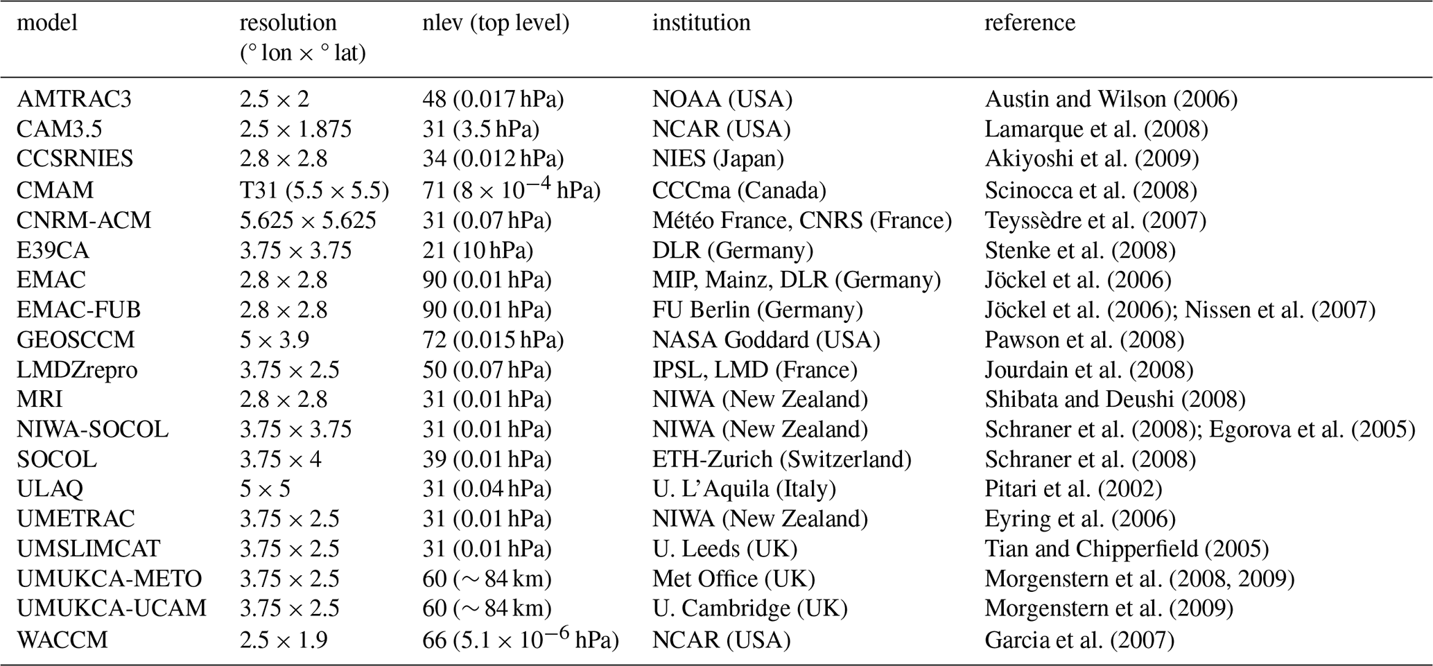
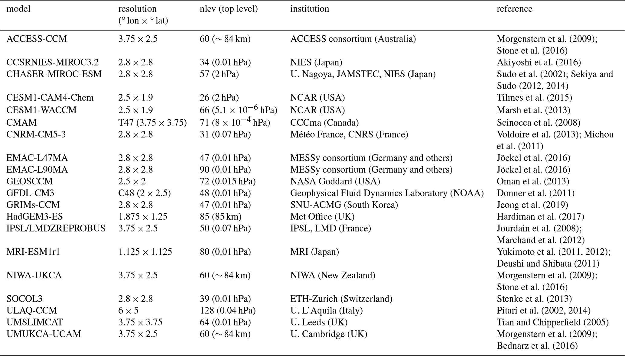
Table A3CCMI-2022 models, resolution, institution and reference.
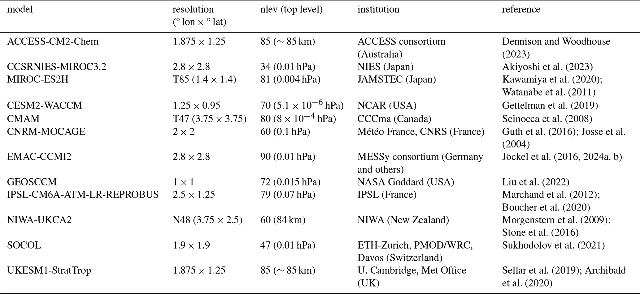
Chemistry-Climate Model output is available online:
-
CCMVal2: https://data.ceda.ac.uk/badc/ccmval/data/CCMVal-2 (last access: 18 April 2026)
-
CCMI: https://data.ceda.ac.uk/badc/wcrp-ccmi/data/CCMI-1/output (last access: 18 April 2026)
-
CCMI-2022: https://data.ceda.ac.uk/badc/ccmi/data/post-cmip6/ccmi-2022 (last access: 18 April 2026)
Satellite and reanalysis data is available online:
-
MLS level2: https://disc.gsfc.nasa.gov/ (last access: 18 April 2026)
-
SWOOSH data are publi Cly available through the web at https://csl.noaa.gov/swoosh (last access: 18 April 2026)
-
Copernicus Climate Change Service (C3S) Climate Data Store (CDS): https://doi.org/10.24381/cds.4ebfe4eb (Copernicus Climate Change Service, 2020).
-
Tropopause dataset Jülich: https://doi.org/10.26165/JUELICH-DATA/UBNGI2 (Hoffmann and Spang, 2021)
-
RID dataset: https://www.jamstec.go.jp/ridinfo/ (last access: 18 April 2026)
-
ACE-FTS: https://databace.scisat.ca/level2/ (last access: 18 April 2026, available via sign-up)
-
satellite-based AoA: https://doi.org/10.5683/SP3/5AC1F0 (Saunders et al., 2025)
The supplement related to this article is available online at https://doi.org/10.5194/acp-26-5249-2026-supplement.
Conceptualization: MA, TB, AC, SDa, AdlC, DH, JK, ML, DM, JN, DP, LS, KS, GS, KT, DW. Formal analysis: MA, AC, SDa, AdlC, HG, OI, JK, ML, DM, LS, KS, KT. Data curation: PM, MC, NLA, HA, MPC, PJ, BJ, MM, OM, TS, SW, YY, SDa, DH, GS. Writing (original draft preparation): MA, TB, SDa, AdlC, MH, ML, DM, DP, LS, KS, DW. Writing (review and editing): All coauthors.
At least one of the (co-)authors is a member of the editorial board of Atmospheric Chemistry and Physics. The peer-review process was guided by an independent editor, and the authors also have no other competing interests to declare.
Publisher's note: Copernicus Publications remains neutral with regard to jurisdictional claims made in the text, published maps, institutional affiliations, or any other geographical representation in this paper. The authors bear the ultimate responsibility for providing appropriate place names. Views expressed in the text are those of the authors and do not necessarily reflect the views of the publisher.
The EMAC simulations have been performed at the German Climate Computing Centre (DKRZ) through support from the Bundesministerium für Bildung und Forschung (BMBF). DKRZ and its scientific steering committee are gratefully acknowledged for providing the HPC and data archiving resources for the consortial project ESCiMo (Earth System Chemistry integrated Modelling). The development of SAGE-CCI-OMPS+ has been supported by the European Space Agency's Climate Change Initiative Ozone ECV Project (CCI, https://climate.esa.int/en/projects/ozone, last access: 18 April 2026); routine generation and procurement of this data record is supported by the Copernicus Climate Change Service (C3S) implemented by the European Centre for Medium-Range Weather Forecasts (ECMWF) on behalf of the European Commission. NEC SX-AURORA TSUBASA at NIES were used to perform CCSRNIES model simulations.
This work has been funded partly by the European Space Agency's Climate Change Initiative Ozone ECV Project, and by the Belgian Federal Science Policy Office (BELSPO) through the Brain-be 2.0 TAPIOWCA project. This research was supported by the International Space Science Institute (ISSI) in Bern, through ISSI International Team project #24-599 (Satellite-Based Evaluation of Stratospheric Transport in Chemistry-Climate Models). MA and OI acknowledge funding from the Spanish national project RecO3very (PID2021-124772OB-I00) and the European Space Agency Contract No. 4000126562/19/I-NB. AC acknowledges funding from the European Research Council within the ERC StG project no. 101078127. SSD and MPC were supported by the Natural Environment Research Council (NERC) LSO3 (NE/V011863/1) and InHALE (NE/X003450/1) projects. SW was supported by MEXT-Program for the advanced studies of climate change projection (SENTAN) Grant Number JPMXD0722681344 and the MIROC-ES2H simulations were performed using the Earth Simulator at JAMSTEC. AdlC acknowledges funding from the Spanish Research Agency grant PID2022‐136316NB‐I00. CCSRNIES modeling group was supported by KAKENHI (JP24K00700, JP24H00751, JP25K07401 and JP25K00377) of the Ministry of Education, Culture, Sports, Science, and Technology, Japan.
This paper was edited by Petr Šácha and reviewed by Kris Wargan and one anonymous referee.
Abalos, M., Legras, B., Ploeger, F., and Randel, W. J.: Evaluating the advective Brewer-Dobson circulation in three reanalyses for the period 1979–2012, J. Geophys. Res.-Atmos., 120, 7534–7554, https://doi.org/10.1002/2015JD023182, 2015. a
Abalos, M., Polvani, L., Calvo, N., Kinnison, D., Ploeger, F., Randel, W., and Solomon, S.: New Insights on the Impact of Ozone-Depleting Substances on the Brewer-Dobson Circulation, J. Geophys. Res.-Atmos., 124, 2435–2451, https://doi.org/10.1029/2018JD029301, 2019. a
Abalos, M., Orbe, C., Kinnison, D. E., Plummer, D., Oman, L. D., Jöckel, P., Morgenstern, O., Garcia, R. R., Zeng, G., Stone, K. A., and Dameris, M.: Future trends in stratosphere-to-troposphere transport in CCMI models, Atmos. Chem. Phys., 20, 6883–6901, https://doi.org/10.5194/acp-20-6883-2020, 2020. a
Abalos, M., Calvo, N., Benito-Barca, S., Garny, H., Hardiman, S. C., Lin, P., Andrews, M. B., Butchart, N., Garcia, R., Orbe, C., Saint-Martin, D., Watanabe, S., and Yoshida, K.: The Brewer–Dobson circulation in CMIP6, Atmos. Chem. Phys., 21, 13571–13591, https://doi.org/10.5194/acp-21-13571-2021, 2021. a, b, c
Acquah, C., Stecher, L., Mertens, M., and Jöckel, P.: Effects of different emission inventories on tropospheric ozone and methane lifetime, Atmos. Chem. Phys., 25, 13665–13686, https://doi.org/10.5194/acp-25-13665-2025, 2025. a
Akinshin, A.: Trimmed Harrell-Davis quantile estimator based on the highest density interval of the given width, Commun. Stat., 53, 1565–1575, https://doi.org/10.1080/03610918.2022.2050396, 2024. a
Akiyoshi, H., Zhou, L. B., Yamashita, Y., Sakamoto, K., Yoshiki, M., Nagashima, T., Takahashi, M., Kurokawa, J., Takigawa, M., and Imamura, T.: A CCM simulation of the breakup of the Antarctic polar vortex in the years 1980–2004 under the CCMVal scenarios, J. Geophys. Res.-Atmos., 114, https://doi.org/10.1029/2007JD009261, 2009. a
Akiyoshi, H., Nakamura, T., Miyasaka, T., Shiotani, M., and Suzuki, M.: A nudged chemistry-climate model simulation of chemical constituent distribution at northern high-latitude stratosphere observed by SMILES and MLS during the 2009/2010 stratospheric sudden warming, J. Geophys. Res.-Atmos., 121, 1361–1380, https://doi.org/10.1002/2015JD023334, 2016. a
Akiyoshi, H., Kadowaki, M., Yamashita, Y., and Nagatomo, T.: Dependence of column ozone on future ODSs and GHGs in the variability of 500-ensemble members, Sci. Rep., 13, 320, https://doi.org/10.1038/s41598-023-27635-y, 2023. a
Andrews, D. G., Holton, J. R., and Leovy, C. B.: Middle Atmosphere Dynamics, Academic Press, San Diego, California, ISBN 9780120585762, 1987. a, b, c
Archibald, A. T., O'Connor, F. M., Abraham, N. L., Archer-Nicholls, S., Chipperfield, M. P., Dalvi, M., Folberth, G. A., Dennison, F., Dhomse, S. S., Griffiths, P. T., Hardacre, C., Hewitt, A. J., Hill, R. S., Johnson, C. E., Keeble, J., Köhler, M. O., Morgenstern, O., Mulcahy, J. P., Ordóñez, C., Pope, R. J., Rumbold, S. T., Russo, M. R., Savage, N. H., Sellar, A., Stringer, M., Turnock, S. T., Wild, O., and Zeng, G.: Description and evaluation of the UKCA stratosphere–troposphere chemistry scheme (StratTrop vn 1.0) implemented in UKESM1, Geosci. Model Dev., 13, 1223–1266, https://doi.org/10.5194/gmd-13-1223-2020, 2020. a
Austin, J. and Wilson, R. J.: Ensemble simulations of the decline and recovery of stratospheric ozone, J. Geophys. Res.-Atmos., 111, https://doi.org/10.1029/2005JD006907, 2006. a
Austin, J., Shindell, D., Beagley, S. R., Brühl, C., Dameris, M., Manzini, E., Nagashima, T., Newman, P., Pawson, S., Pitari, G., Rozanov, E., Schnadt, C., and Shepherd, T. G.: Uncertainties and assessments of chemistry-climate models of the stratosphere, Atmos. Chem. Phys., 3, 1–27, https://doi.org/10.5194/acp-3-1-2003, 2003. a
Bednarz, E. M., Maycock, A. C., Abraham, N. L., Braesicke, P., Dessens, O., and Pyle, J. A.: Future Arctic ozone recovery: the importance of chemistry and dynamics, Atmos. Chem. Phys., 16, 12159–12176, https://doi.org/10.5194/acp-16-12159-2016, 2016. a
Bernath, P. F., McElroy, C. T., Abrams, M. C., Boone, C. D., Butler, M., Camy-Peyret, C., Carleer, M., Clerbaux, C., Coheur, P.-F., Colin, R., DeCola, P., DeMazière, M., Drummond, J. R., Dufour, D., Evans, W. F. J., Fast, H., Fussen, D., Gilbert, K., Jennings, D. E., Llewellyn, E. J., Lowe, R. P., Mahieu, E., McConnell, J. C., McHugh, M., McLeod, S. D., Michaud, R., Midwinter, C., Nassar, R., Nichitiu, F., Nowlan, C., Rinsland, C. P., Rochon, Y. J., Rowlands, N., Semeniuk, K., Simon, P., Skelton, R., Sloan, J. J., Soucy, M.-A., Strong, K., Tremblay, P., Turnbull, D., Walker, K. A., Walkty, I., Wardle, D. A., Wehrle, V., Zander, R., and Zou, J.: Atmospheric Chemistry Experiment (ACE): Mission overview, Geophys. Res. Lett., 32, https://doi.org/10.1029/2005GL022386, 2005. a
Boone, C. D.: Version 3 Retrievals for the Atmospheric Chemistry Experiment Fourier Transform Spectrometer (ACE-FTS), https://api.semanticscholar.org/CorpusID:221710947 (last access: 18 April 2026), 2020. a
Boone, C. D., Walker, K. A., and Bernath, P. F.: Version 3 retrievals for the Atmospheric Chemistry Experiment Fourier Transform Spectrometer (ACE-FTS), in: ACE at 10: A Solar Occultation Anthology, Deepak Publishing, ISBN 978-0-937194-54-9, 2013. a
Boucher, O., Servonnat, J., Albright, A. L., Aumont, O., Balkanski, Y., Bastrikov, V., Bekki, S., Bonnet, R., Bony, S., Bopp, L., Braconnot, P., Brockmann, P., Cadule, P., Caubel, A., Cheruy, F., Codron, F., Cozic, A., Cugnet, D., D'Andrea, F., Davini, P., de Lavergne, C., Denvil, S., Deshayes, J., Devilliers, M., Ducharne, A., Dufresne, J.-L., Dupont, E., Éthé, C., Fairhead, L., Falletti, L., Flavoni, S., Foujols, M.-A., Gardoll, S., Gastineau, G., Ghattas, J., Grandpeix, J.-Y., Guenet, B., Guez, Lionel, E., Guilyardi, E., Guimberteau, M., Hauglustaine, D., Hourdin, F., Idelkadi, A., Joussaume, S., Kageyama, M., Khodri, M., Krinner, G., Lebas, N., Levavasseur, G., Lévy, C., Li, L., Lott, F., Lurton, T., Luyssaert, S., Madec, G., Madeleine, J.-B., Maignan, F., Marchand, M., Marti, O., Mellul, L., Meurdesoif, Y., Mignot, J., Musat, I., Ottlé, C., Peylin, P., Planton, Y., Polcher, J., Rio, C., Rochetin, N., Rousset, C., Sepulchre, P., Sima, A., Swingedouw, D., Thiéblemont, R., Traore, A. K., Vancoppenolle, M., Vial, J., Vialard, J., Viovy, N., and Vuichard, N.: Presentation and Evaluation of the IPSL-CM6A-LR Climate Model, J. Adv. Model. Earth Sy., 12, e2019MS002010, https://doi.org/10.1029/2019MS002010, 2020. a
Brewer, A. W.: Evidence for a world circulation provided by the measurements of helium and water vapour distribution in the stratosphere, Q. J. Roy. Meteor. Soc., 75, 351–363, https://doi.org/10.1002/qj.49707532603, 1949. a
Chipperfield, M. P.: New version of the TOMCAT/SLIMCAT off-line chemical transport model: Intercomparison of stratospheric tracer experiments, Q. J. Roy. Meteor. Soc., 132, 1179–1203, https://doi.org/10.1256/qj.05.51, 2006. a
Chipperfield, M. P., Dhomse, S., Hossaini, R., Feng, W., Santee, M. L., Weber, M., Burrows, J. P., Wild, J. D., Loyola, D., and Coldewey-Egbers, M.: On the Cause of Recent Variations in Lower Stratospheric Ozone, Geophys. Res. Lett., 45, 5718–5726, https://doi.org/10.1029/2018GL078071, 2018. a
Chipperfield, M. P., Santee, M. L. (lead authors), Alexander, S. P., de Laat, A. T. J., Kinnison, D. E., Kuttippurath, J., Langematz, U., and Wargan, K.: Polar Stratospheric Ozone: Past, Present, and Future, in: Scientific Assessment of Ozone Depletion: 2022, chap. 4, World Meteorological Organization, Geneva, ISBN 978-9914-733-97-6, 2022. a
Coddington, O., Lean, J., Pilewskie, P., Snow, M., Richard, E., Kopp, G., Lindholm, C., DeLand, M., Marchenko, S., Haberreiter, M., and Baranyi, T.: Solar Irradiance Variability: Comparisons of Models and Measurements, Earth Space Sci., 6, 2525–2555, https://doi.org/10.1029/2019EA000693, 2019. a
Copernicus Climate Change Service: Ozone monthly gridded data from 1970 to present derived from satellite observations, Copernicus Climate Change Service (C3S) Climate Data Store (CDS) [dadta set], https://doi.org/10.24381/cds.4ebfe4eb, 2020. a
Davis, S. M., Rosenlof, K. H., Hassler, B., Hurst, D. F., Read, W. G., Vömel, H., Selkirk, H., Fujiwara, M., and Damadeo, R.: The Stratospheric Water and Ozone Satellite Homogenized (SWOOSH) database: a long-term database for climate studies, Earth Syst. Sci. Data, 8, 461–490, https://doi.org/10.5194/essd-8-461-2016, 2016. a
de la Cámara, A., Lott, F., and Abalos, M.: Climatology of the middle atmosphere in LMDz: Impact of source-related parameterizations of gravity wave drag, J. Adv. Model. Earth Sy., 8, 1507–1525, https://doi.org/10.1002/2016MS000753, 2016. a
Dennison, F. and Woodhouse, M. T.: ACCESS-CM2-Chem: evaluation of southern hemisphere ozone and its effect on the Southern Annular Mode, Journal of Southern Hemisphere Earth Systems Science, 73, 17–29, https://doi.org/10.1071/ES22015, 2023. a
Deushi, M. and Shibata, K.: Development of a Meteorological Research Institute Chemistry-Climate Model version 2 for the Study of Tropospheric and Stratospheric Chemistry, Pap. Meteorol. Geophys., 62, 1–46, https://doi.org/10.2467/mripapers.62.1, 2011. a
Dhomse, S. S., Feng, W., Montzka, S. A., Hossaini, R., Keeble, J., Pyle, J. A., Daniel, J. S., and Chipperfield, M. P.: Delay in recovery of the Antarctic ozone hole from unexpected CFC-11 emissions, Nat. Commun., 10, 5781, https://doi.org/10.1038/s41467-019-13717-x, 2019. a
Diallo, M., Ern, M., and Ploeger, F.: The advective Brewer–Dobson circulation in the ERA5 reanalysis: climatology, variability, and trends, Atmos. Chem. Phys., 21, 7515–7544, https://doi.org/10.5194/acp-21-7515-2021, 2021. a
Dietmüller, S., Eichinger, R., Garny, H., Birner, T., Boenisch, H., Pitari, G., Mancini, E., Visioni, D., Stenke, A., Revell, L., Rozanov, E., Plummer, D. A., Scinocca, J., Jöckel, P., Oman, L., Deushi, M., Kiyotaka, S., Kinnison, D. E., Garcia, R., Morgenstern, O., Zeng, G., Stone, K. A., and Schofield, R.: Quantifying the effect of mixing on the mean age of air in CCMVal-2 and CCMI-1 models, Atmos. Chem. Phys., 18, 6699–6720, https://doi.org/10.5194/acp-18-6699-2018, 2018. a, b, c, d, e, f, g, h, i
Dobson, G. M. B.: Origin and distribution of the polyatomic molecules in the atmosphere, P. Roy. Soc. A.-Math. Phy., 236, 187–193, https://doi.org/10.1098/rspa.1956.0127, 1956. a
Donner, L. J., Wyman, B. L., Hemler, R. S., Horowitz, L. W., Ming, Y., Zhao, M., Golaz, J.-C., Ginoux, P., Lin, S.-J., Schwarzkopf, M. D., Austin, J., Alaka, G., Cooke, W. F., Delworth, T. L., Freidenreich, S. M., Gordon, C. T., Griffies, S. M., Held, I. M., Hurlin, W. J., Klein, S. A., Knutson, T. R., Langenhorst, A. R., Lee, H.-C., Lin, Y., Magi, B. I., Malyshev, S. L., Milly, P. C. D., Naik, V., Nath, M. J., Pincus, R., Ploshay, J. J., Ramaswamy, V., Seman, C. J., Shevliakova, E., Sirutis, J. J., Stern, W. F., Stouffer, R. J., Wilson, R. J., Winton, M., Wittenberg, A. T., and Zeng, F.: The Dynamical Core, Physical Parameterizations, and Basic Simulation Characteristics of the Atmospheric Component AM3 of the GFDL Global Coupled Model CM3, J. Climate, 24, 3484–3519, https://doi.org/10.1175/2011JCLI3955.1, 2011. a
Douglass, A. R., Stolarski, R. S., Schoeberl, M. R., Jackman, C. H., Gupta, M. L., Newman, P. A., Nielsen, J. E., and Fleming, E. L.: Relationship of loss, mean age of air and the distribution of CFCs to stratospheric circulation and implications for atmospheric lifetimes, J. Geophys. Res.-Atmos., 113, https://doi.org/10.1029/2007JD009575, 2008. a
Douglass, A. R., Prather, M. J., Hall, T. M., Strahan, S. E., Rasch, P. J., Sparling, L. C., Coy, L., and Rodriguez, J. M.: Choosing meteorological input for the global modeling initiative assessment of high-speed aircraft, J. Geophys. Res.-Atmos., 104, 27545–27564, https://doi.org/10.1029/1999JD900827, 1999. a
Dubé, K., Tegtmeier, S., Bourassa, A., Zawada, D., Degenstein, D., Sheese, P. E., Walker, K. A., and Randel, W.: N2O as a regression proxy for dynamical variability in stratospheric trace gas trends, Atmos. Chem. Phys., 23, 13283–13300, https://doi.org/10.5194/acp-23-13283-2023, 2023. a
Egorova, T., Rozanov, E., Zubov, V., Manzini, E., Schmutz, W., and Peter, T.: Chemistry-climate model SOCOL: a validation of the present-day climatology, Atmos. Chem. Phys., 5, 1557–1576, https://doi.org/10.5194/acp-5-1557-2005, 2005. a
Eichinger, R., Dietmüller, S., Garny, H., Šácha, P., Birner, T., Bönisch, H., Pitari, G., Visioni, D., Stenke, A., Rozanov, E., Revell, L., Plummer, D. A., Jöckel, P., Oman, L., Deushi, M., Kinnison, D. E., Garcia, R., Morgenstern, O., Zeng, G., Stone, K. A., and Schofield, R.: The influence of mixing on the stratospheric age of air changes in the 21st century, Atmos. Chem. Phys., 19, 921–940, https://doi.org/10.5194/acp-19-921-2019, 2019. a, b
Engel, A., Bönisch, H., Ostermöller, J., Chipperfield, M. P., Dhomse, S., and Jöckel, P.: A refined method for calculating equivalent effective stratospheric chlorine, Atmos. Chem. Phys., 18, 601–619, https://doi.org/10.5194/acp-18-601-2018, 2018. a
Eyring, V., Butchart, N., Waugh, D. W., Akiyoshi, H., Austin, J., Bekki, S., Bodeker, G. E., Boville, B. A., Brühl, C., Chipperfield, M. P., Cordero, E., Dameris, M., Deushi, M., Fioletov, V. E., Frith, S. M., Garcia, R. R., Gettelman, A., Giorgetta, M. A., Grewe, V., Jourdain, L., Kinnison, D. E., Mancini, E., Manzini, E., Marchand, M., Marsh, D. R., Nagashima, T., Newman, P. A., Nielsen, J. E., Pawson, S., Pitari, G., Plummer, D. A., Rozanov, E., Schraner, M., Shepherd, T. G., Shibata, K., Stolarski, R. S., Struthers, H., Tian, W., and Yoshiki, M.: Assessment of temperature, trace species, and ozone in chemistry-climate model simulations of the recent past, J. Geophys. Res.-Atmos., 111, https://doi.org/10.1029/2006JD007327, 2006. a, b, c, d
Eyring, V., Lamarque, J.-F., Hess, P., Arfeuille, F., Bowman, K., Chipperfield, M. P., Duncan, B., Fiore, A., Gettelman, A., Giorgetta, M. A., Granier, C., Hegglin, M., Kinnison, D., Kunze, M., Langematz, U., Luo, B., Martin, R., Matthes, K., Newman, P. A., Peter, T., Robock, A., Ryerson, T., Saiz-Lopez, A., Salawitch, R., Schultz, M., Shepherd, T. G., Shindell, D., Stahelin, J., Tegtmeier, S., Thomason, L., Tilmes, S., Vernier, J.-P., Waugh, D. W., and Young, P. J.: Overview of IGAC/SPARC Chemistry–Climate Model Initiative (CCMI) Community Simulations in Support of Upcoming Ozone and Climate Assessments, SPARC Newsletter, 40, 48–66, 2013. a, b
Feng, W., Dhomse, S. S., Arosio, C., Weber, M., Burrows, J. P., Santee, M. L., and Chipperfield, M. P.: Arctic Ozone Depletion in 2019/20: Roles of Chemistry, Dynamics and the Montreal Protocol, Geophys. Res. Lett., 48, e2020GL091911, https://doi.org/10.1029/2020GL091911, 2021. a
Fischer, H., Birk, M., Blom, C., Carli, B., Carlotti, M., von Clarmann, T., Delbouille, L., Dudhia, A., Ehhalt, D., Endemann, M., Flaud, J. M., Gessner, R., Kleinert, A., Koopman, R., Langen, J., López-Puertas, M., Mosner, P., Nett, H., Oelhaf, H., Perron, G., Remedios, J., Ridolfi, M., Stiller, G., and Zander, R.: MIPAS: an instrument for atmospheric and climate research, Atmos. Chem. Phys., 8, 2151–2188, https://doi.org/10.5194/acp-8-2151-2008, 2008. a
Fujiwara, M., Martineau, P., Wright, J. S., Abalos, M., Šácha, P., Kawatani, Y., Davis, S. M., Birner, T., and Monge-Sanz, B. M.: Climatology of the terms and variables of transformed Eulerian-mean (TEM) equations from multiple reanalyses: MERRA-2, JRA-55, ERA-Interim, and CFSR, Atmos. Chem. Phys., 24, 7873–7898, https://doi.org/10.5194/acp-24-7873-2024, 2024. a
Garcia, R. R., Marsh, D. R., Kinnison, D. E., Boville, B. A., and Sassi, F.: Simulation of secular trends in the middle atmosphere, 1950–2003, J. Geophys. Res.-Atmos., 112, https://doi.org/10.1029/2006JD007485, 2007. a
Garny, H., Birner, T., Bönisch, H., and Bunzel, F.: The effects of mixing on age of air, J. Geophys. Res.-Atmos., 119, 7015–7034, https://doi.org/10.1002/2013JD021417, 2014. a, b, c, d
Garny, H., Eichinger, R., Laube, J. C., Ray, E. A., Stiller, G. P., Bönisch, H., Saunders, L., and Linz, M.: Correction of stratospheric age of air (AoA) derived from sulfur hexafluoride (SF6) for the effect of chemical sinks, Atmos. Chem. Phys., 24, 4193–4215, https://doi.org/10.5194/acp-24-4193-2024, 2024a. a
Garny, H., Ploeger, F., Abalos, M., Bönisch, H., Castillo, A. E., von Clarmann, T., Diallo, M., Engel, A., Laube, J. C., Linz, M., Neu, J. L., Podglajen, A., Ray, E., Rivoire, L., Saunders, L. N., Stiller, G., Voet, F., Wagenhäuser, T., and Walker, K. A.: Age of Stratospheric Air: Progress on Processes, Observations, and Long-Term Trends, Rev. Geophys., 62, e2023RG000832, https://doi.org/10.1029/2023RG000832, 2024b. a, b, c, d, e, f, g, h, i
Gelaro, R., McCarty, W., Suárez, M. J., Todling, R., Molod, A., Takacs, L., Randles, C. A., Darmenov, A., Bosilovich, M. G., Reichle, R., Wargan, K., Coy, L., Cullather, R., Draper, C., Akella, S., Buchard, V., Conaty, A., da Silva, A. M., Gu, W., Kim, G.-K., Koster, R., Lucchesi, R., Merkova, D., Nielsen, J. E., Partyka, G., Pawson, S., Putman, W., Rienecker, M., Schubert, S. D., Sienkiewicz, M., and Zhao, B.: The Modern-Era Retrospective Analysis for Research and Applications, Version 2 (MERRA-2), J. Climate, 30, 5419–5454, https://doi.org/10.1175/JCLI-D-16-0758.1, 2017. a
Gettelman, A., Hegglin, M. I., Son, S.-W., Kim, J., Fujiwara, M., Birner, T., Kremser, S., Rex, M., Añel, J. A., Akiyoshi, H., Austin, J., Bekki, S., Braesike, P., Brühl, C., Butchart, N., Chipperfield, M., Dameris, M., Dhomse, S., Garny, H., Hardiman, S. C., Jöckel, P., Kinnison, D. E., Lamarque, J. F., Mancini, E., Marchand, M., Michou, M., Morgenstern, O., Pawson, S., Pitari, G., Plummer, D., Pyle, J. A., Rozanov, E., Scinocca, J., Shepherd, T. G., Shibata, K., Smale, D., Teyssèdre, H., and Tian, W.: Multimodel assessment of the upper troposphere and lower stratosphere: Tropics and global trends, J. Geophys. Res.-Atmos., 115, https://doi.org/10.1029/2009JD013638, 2010. a, b, c, d
Gettelman, A., Mills, M. J., Kinnison, D. E., Garcia, R. R., Smith, A. K., Marsh, D. R., Tilmes, S., Vitt, F., Bardeen, C. G., McInerny, J., Liu, H.-L., Solomon, S. C., Polvani, L. M., Emmons, L. K., Lamarque, J.-F., Richter, J. H., Glanville, A. S., Bacmeister, J. T., Phillips, A. S., Neale, R. B., Simpson, I. R., DuVivier, A. K., Hodzic, A., and Randel, W. J.: The Whole Atmosphere Community Climate Model Version 6 (WACCM6), J. Geophys. Res.-Atmos/, 124, 12380–12403, https://doi.org/10.1029/2019JD030943, 2019. a
Glanville, A. A. and Birner, T.: Role of vertical and horizontal mixing in the tape recorder signal near the tropical tropopause, Atmos. Chem. Phys., 17, 4337–4353, https://doi.org/10.5194/acp-17-4337-2017, 2017. a
Glatthor, N., von Clarmann, T., Funke, B., García-Comas, M., Grabowski, U., Höpfner, M., Kellmann, S., Kiefer, M., Laeng, A., Linden, A., López-Puertas, M., and Stiller, G. P.: IMK–IAA MIPAS retrieval version 8: CH4 and N2O, Atmos. Meas. Tech., 17, 2849–2871, https://doi.org/10.5194/amt-17-2849-2024, 2024. a
GloSSAC: Global Space-based Stratospheric Aerosol Climatology Version 2.0, NASA Langley Atmospheric Science Data Center DAAC [data set], https://doi.org/10.5067/GLOSSAC-L3-V2.0, 2018. a
Godin-Beekmann, S., Azouz, N., Sofieva, V. F., Hubert, D., Petropavlovskikh, I., Effertz, P., Ancellet, G., Degenstein, D. A., Zawada, D., Froidevaux, L., Frith, S., Wild, J., Davis, S., Steinbrecht, W., Leblanc, T., Querel, R., Tourpali, K., Damadeo, R., Maillard Barras, E., Stübi, R., Vigouroux, C., Arosio, C., Nedoluha, G., Boyd, I., Van Malderen, R., Mahieu, E., Smale, D., and Sussmann, R.: Updated trends of the stratospheric ozone vertical distribution in the 60° S–60° N latitude range based on the LOTUS regression model , Atmos. Chem. Phys., 22, 11657–11673, https://doi.org/10.5194/acp-22-11657-2022, 2022. a, b
Guth, J., Josse, B., Marécal, V., Joly, M., and Hamer, P.: First implementation of secondary inorganic aerosols in the MOCAGE version R2.15.0 chemistry transport model, Geosci. Model Dev., 9, 137–160, https://doi.org/10.5194/gmd-9-137-2016, 2016. a
Haenel, F. J., Stiller, G. P., von Clarmann, T., Funke, B., Eckert, E., Glatthor, N., Grabowski, U., Kellmann, S., Kiefer, M., Linden, A., and Reddmann, T.: Reassessment of MIPAS age of air trends and variability, Atmos. Chem. Phys., 15, 13161–13176, https://doi.org/10.5194/acp-15-13161-2015, 2015. a
Hall, T. M. and Plumb, R. A.: Age as a diagnostic of stratospheric transport, J. Geophys. Res.-Atmos., 99, 1059–1070, https://doi.org/10.1029/93JD03192, 1994. a
Hall, T. M., Waugh, D. W., Boering, K. A., and Plumb, R. A.: Evaluation of transport in stratospheric models, J. Geophys. Res.-Atmos., 104, 18815–18839, https://doi.org/10.1029/1999JD900226, 1999. a, b
Hardiman, S. C., Butchart, N., and Calvo, N.: The morphology of the Brewer–Dobson circulation and its response to climate change in CMIP5 simulations, Q. J. Roy. Meteor. Soc., 140, 1958–1965, https://doi.org/10.1002/qj.2258, 2014. a, b
Hardiman, S. C., Butchart, N., O'Connor, F. M., and Rumbold, S. T.: The Met Office HadGEM3-ES chemistry–climate model: evaluation of stratospheric dynamics and its impact on ozone, Geosci. Model Dev., 10, 1209–1232, https://doi.org/10.5194/gmd-10-1209-2017, 2017. a
Harrison, J. J.: New infrared absorption cross sections for the infrared limb sounding of sulfur hexafluoride (SF6), J. Quant. Spectrosc. Ra., 254, 107202, https://doi.org/10.1016/j.jqsrt.2020.107202, 2020. a
Hegglin, M. I., Gettelman, A., Hoor, P., Krichevsky, R., Manney, G. L., Pan, L. L., Son, S.-W., Stiller, G., Tilmes, S., Walker, K. A., Eyring, V., Shepherd, T. G., Waugh, D., Akiyoshi, H., Añel, J. A., Austin, J., Baumgaertner, A., Bekki, S., Braesicke, P., Brühl, C., Butchart, N., Chipperfield, M., Dameris, M., Dhomse, S., Frith, S., Garny, H., Hardiman, S. C., Jöckel, P., Kinnison, D. E., Lamarque, J. F., Mancini, E., Michou, M., Morgenstern, O., Nakamura, T., Olivié, D., Pawson, S., Pitari, G., Plummer, D. A., Pyle, J. A., Rozanov, E., Scinocca, J. F., Shibata, K., Smale, D., Teyssèdre, H., Tian, W., and Yamashita, Y.: Multimodel assessment of the upper troposphere and lower stratosphere: Extratropics, J. Geophys. Res.-Atmos., 115, https://doi.org/10.1029/2010JD013884, 2010. a
Hersbach, H., Bell, B., Berrisford, P., Hirahara, S., Horányi, A., Muñoz-Sabater, J., Nicolas, J., Peubey, C., Radu, R., Schepers, D., Simmons, A., Soci, C., Abdalla, S., Abellan, X., Balsamo, G., Bechtold, P., Biavati, G., Bidlot, J., Bonavita, M., De Chiara, G., Dahlgren, P., Dee, D., Diamantakis, M., Dragani, R., Flemming, J., Forbes, R., Fuentes, M., Geer, A., Haimberger, L., Healy, S., Hogan, R. J., Hólm, E., Janisková, M., Keeley, S., Laloyaux, P., Lopez, P., Lupu, C., Radnoti, G., de Rosnay, P., Rozum, I., Vamborg, F., Villaume, S., and Thépaut, J.-N.: The ERA5 global reanalysis, Q. J. Roy. Meteor. Soc., 146, 1999–2049, https://doi.org/10.1002/qj.3803, 2020. a, b
Hoffmann, L. and Spang, R.: Reanalysis Tropopause Data Repository, Juelich DATA [data set], https://doi.org/10.26165/JUELICH-DATA/UBNGI2, 2021. a
Hoffmann, L. and Spang, R.: An assessment of tropopause characteristics of the ERA5 and ERA-Interim meteorological reanalyses, Atmos. Chem. Phys., 22, 4019–4046, https://doi.org/10.5194/acp-22-4019-2022, 2022. a
Hubert, D., Lambert, J.-C., Verhoelst, T., Granville, J., Keppens, A., Baray, J.-L., Bourassa, A. E., Cortesi, U., Degenstein, D. A., Froidevaux, L., Godin-Beekmann, S., Hoppel, K. W., Johnson, B. J., Kyrölä, E., Leblanc, T., Lichtenberg, G., Marchand, M., McElroy, C. T., Murtagh, D., Nakane, H., Portafaix, T., Querel, R., Russell III, J. M., Salvador, J., Smit, H. G. J., Stebel, K., Steinbrecht, W., Strawbridge, K. B., Stübi, R., Swart, D. P. J., Taha, G., Tarasick, D. W., Thompson, A. M., Urban, J., van Gijsel, J. A. E., Van Malderen, R., von der Gathen, P., Walker, K. A., Wolfram, E., and Zawodny, J. M.: Ground-based assessment of the bias and long-term stability of 14 limb and occultation ozone profile data records, Atmos. Meas. Tech., 9, 2497–2534, https://doi.org/10.5194/amt-9-2497-2016, 2016. a
Hurst, D. F., Read, W. G., Vömel, H., Selkirk, H. B., Rosenlof, K. H., Davis, S. M., Hall, E. G., Jordan, A. F., and Oltmans, S. J.: Recent divergences in stratospheric water vapor measurements by frost point hygrometers and the Aura Microwave Limb Sounder, Atmos. Meas. Tech., 9, 4447–4457, https://doi.org/10.5194/amt-9-4447-2016, 2016. a
Jeong, Y.-C., Yeh, S.-W., Lee, S., and Park, R. J.: A Global/Regional Integrated Model System-Chemistry Climate Model: 1. Simulation Characteristics, Earth Space Sci., 6, 2016–2030, https://doi.org/10.1029/2019EA000727, 2019. a
Jöckel, P., Tost, H., Pozzer, A., Brühl, C., Buchholz, J., Ganzeveld, L., Hoor, P., Kerkweg, A., Lawrence, M. G., Sander, R., Steil, B., Stiller, G., Tanarhte, M., Taraborrelli, D., van Aardenne, J., and Lelieveld, J.: The atmospheric chemistry general circulation model ECHAM5/MESSy1: consistent simulation of ozone from the surface to the mesosphere, Atmos. Chem. Phys., 6, 5067–5104, https://doi.org/10.5194/acp-6-5067-2006, 2006. a, b
Jöckel, P., Tost, H., Pozzer, A., Kunze, M., Kirner, O., Brenninkmeijer, C. A. M., Brinkop, S., Cai, D. S., Dyroff, C., Eckstein, J., Frank, F., Garny, H., Gottschaldt, K.-D., Graf, P., Grewe, V., Kerkweg, A., Kern, B., Matthes, S., Mertens, M., Meul, S., Neumaier, M., Nützel, M., Oberländer-Hayn, S., Ruhnke, R., Runde, T., Sander, R., Scharffe, D., and Zahn, A.: Earth System Chemistry integrated Modelling (ESCiMo) with the Modular Earth Submodel System (MESSy) version 2.51, Geosci. Model Dev., 9, 1153–1200, https://doi.org/10.5194/gmd-9-1153-2016, 2016. a, b, c
Jöckel, P., Brinkop, S., Graf, P., Eichinger, R., Garny, H., Mertens, M., Nützel, M., Pozzer, A., Tost, H., and Consortium, T. M.: RD1: EMAC CCMI-2022 free running hindcast simulation 1950–2019, World Data Center for Climate [data set], https://doi.org/10.26050/WDCC/ESCiMo2_RD1, 2024a. a
Jöckel, P., Brinkop, S., Graf, P., Eichinger, R., Garny, H., Mertens, M., Nützel, M., Pozzer, A., Tost, H., and MESSy Consortium, T.: RD1: EMAC CCMI-2022 free running hindcast simulation 1950-2019 (additional data), https://www.wdc-climate.de/ui/entry?acronym=DKRZ_LTA_853_dsg0001 (last access: 18 April 2026), 2024b. a
Josse, B., Simon, P., and Peuch, V.-H.: Radon global simulations with the multiscale chemistry and transport model MOCAGE, Tellus B, 56, 339–356, https://doi.org/10.1111/j.1600-0889.2004.00112.x, 2004. a
Jourdain, L., Bekki, S., Lott, F., and Lefèvre, F.: The coupled chemistry-climate model LMDz-REPROBUS: description and evaluation of a transient simulation of the period 1980–1999, Ann. Geophys., 26, 1391–1413, https://doi.org/10.5194/angeo-26-1391-2008, 2008. a, b
Kawamiya, M., Hajima, T., Tachiiri, K., Watanabe, S., and Yokohata, T.: Two decades of Earth system modeling with an emphasis on Model for Interdisciplinary Research on Climate (MIROC), Prog. Earth Planet. Sci., 7, 64, https://doi.org/10.1186/s40645-020-00369-5, 2020. a
Ko, M. K. W., Jackman, C. H., Plumb, R. A., Kaye, J. A., and Sage, K. H.: The atmosphere effects of stratospheric aircraft: Reports of the 1998 Models and Measurements II Workshop, Tech. Rep. NASA Technical Memorandum 1991–209554, edited by: Park, J., National Aeronautics and Space Administration, NASA/TM—1999-209554, 1999. a
Kobayashi, C. and Iwasaki, T.: The Brewer–Dobson circulation in the JRA-3Q reanalysis and the impact of changes in model physical processes, Q. J. Roy. Meteor. Soc., 150, 5605–5620, https://doi.org/10.1002/qj.4896, 2024. a
Kosaka, Y., Kobayashi, S., Harada, Y., Kobayashi, C., Naoe, H., Yoshimoto, K., Harada, M., Goto, N., Chiba, J., Miyaoka, K., Sekiguchi, R., Deushi, M., Kamahori, H., Nakaegawa, T., Tanaka, T. Y., Tokuhiro, T., Sato, Y., Matsushita, Y., and Onogi, K.: The JRA-3Q Reanalysis, J. Meteorol. Soc. Jpn. Ser. II, 102, 49–109, https://doi.org/10.2151/jmsj.2024-004, 2024. a
Lamarque, J.-F., Kinnison, D. E., Hess, P. G., and Vitt, F. M.: Simulated lower stratospheric trends between 1970 and 2005: Identifying the role of climate and composition changes, J. Geophys. Res.-Atmos., 113, https://doi.org/10.1029/2007JD009277, 2008. a
Lickley, M. J., Daniel, J. S., McBride, L. A., Salawitch, R. J., and Velders, G. J. M.: The return to 1980 stratospheric halogen levels: a moving target in ozone assessments from 2006 to 2022, Atmos. Chem. Phys., 24, 13081–13099, https://doi.org/10.5194/acp-24-13081-2024, 2024. a, b, c
Linz, M., Plumb, R. A., Gerber, E. P., and Sheshadri, A.: The Relationship between Age of Air and the Diabatic Circulation of the Stratosphere, J. Atmos. Sci., 73, 4507–4518, https://doi.org/10.1175/JAS-D-16-0125.1, 2016. a, b, c
Linz, M., Abalos, M., Glanville, A. S., Kinnison, D. E., Ming, A., and Neu, J. L.: The global diabatic circulation of the stratosphere as a metric for the Brewer–Dobson circulation, Atmos. Chem. Phys., 19, 5069–5090, https://doi.org/10.5194/acp-19-5069-2019, 2019. a
Linz, M., Plumb, R. A., Gupta, A., and Gerber, E. P.: Stratospheric Adiabatic Mixing Rates Derived From the Vertical Gradient of Age of Air, J. Geophys. Res.-Atmos., 126, e2021JD035199, https://doi.org/10.1029/2021JD035199, 2021. a, b, c, d, e
Liu, J., Strode, S. A., Liang, Q., Oman, L. D., Colarco, P. R., Fleming, E. L., Manyin, M. E., Douglass, A. R., Ziemke, J. R., Lamsal, L. N., and Li, C.: Change in Tropospheric Ozone in the Recent Decades and Its Contribution to Global Total Ozone, J. Geophys. Res.-Atmos., 127, e2022JD037170, https://doi.org/10.1029/2022JD037170, 2022. a
Livesey, N. J., Read, W. G., Froidevaux, L., Lambert, A., Santee, M. L., Schwartz, M. J., Millán, L. F., Jarnot, R. F., Wagner, P. A., Hurst, D. F., Walker, K. A., Sheese, P. E., and Nedoluha, G. E.: Investigation and amelioration of long-term instrumental drifts in water vapor and nitrous oxide measurements from the Aura Microwave Limb Sounder (MLS) and their implications for studies of variability and trends, Atmos. Chem. Phys., 21, 15409–15430, https://doi.org/10.5194/acp-21-15409-2021, 2021. a
Livesey, N. J., Read, W. G., Wagner, P. A., Froidevaux, L., Santee, M. L., Schwartz, M. J., Lambert, A., Millan Valle, L. F., Pumphrey, H. C., Manney, G. L., Fuller, R. A., Jarnot, R. F., Knosp, B. W., and Lay, R. R.: Earth Observing System (EOS) Microwave Limb Sounder (MLS) Version 5.0x Level 2 and 3 data quality and description document, https://doi.org/10.5067/AURA/MLS/DOC/V5_DATAQUALITYDOCUMENT, 2022. a, b
Loeffel, S., Eichinger, R., Garny, H., Reddmann, T., Fritsch, F., Versick, S., Stiller, G., and Haenel, F.: The impact of sulfur hexafluoride (SF6) sinks on age of air climatologies and trends, Atmos. Chem. Phys., 22, 1175–1193, https://doi.org/10.5194/acp-22-1175-2022, 2022. a
Luo, B.: Stratospheric aerosol data for use in CMIP6 models, dataset documentation, ftp://iacftp.ethz.ch/pub_read/luo/CMIP6/Readme_Data_Description.pdf (last access: 1 April 2020), 2016. a
Marchand, M., Keckhut, P., Lefebvre, S., Claud, C., Cugnet, D., Hauchecorne, A., Lefèvre, F., Lefebvre, M.-P., Jumelet, J., Lott, F., Hourdin, F., Thuillier, G., Poulain, V., Bossay, S., Lemennais, P., David, C., and Bekki, S.: Dynamical amplification of the stratospheric solar response simulated with the Chemistry-Climate Model LMDz-Reprobus, J. Atmos. Sol.-Terr. Phys., 75–76, 147–160, https://doi.org/10.1016/j.jastp.2011.11.008, 2012. a, b
Marsh, D. R., Mills, M. J., Kinnison, D. E., Lamarque, J.-F., Calvo, N., and Polvani, L. M.: Climate Change from 1850 to 2005 Simulated in CESM1(WACCM), J. Climate, 26, 7372–7391, https://doi.org/10.1175/JCLI-D-12-00558.1, 2013. a
Martineau, P., Wright, J. S., Zhu, N., and Fujiwara, M.: Zonal-mean data set of global atmospheric reanalyses on pressure levels, Earth Syst. Sci. Data, 10, 1925–1941, https://doi.org/10.5194/essd-10-1925-2018, 2018. a
McIntyre, M. and Palmer, T.: The “surf zone” in the stratosphere, J. Atmos. Terr. Phys., 46, 825–849, https://doi.org/10.1016/0021-9169(84)90063-1, 1984. a
McLandress, C., Jonsson, A. I., Plummer, D. A., Reader, M. C., Scinocca, J. F., and Shepherd, T. G.: Separating the Dynamical Effects of Climate Change and Ozone Depletion. Part I: Southern Hemisphere Stratosphere, J. Climate, 23, 5002–5020, https://doi.org/10.1175/2010JCLI3586.1, 2010. a, b
McLandress, C., Shepherd, T. G., Polavarapu, S., and Beagley, S. R.: Is Missing Orographic Gravity Wave Drag near 60°S the Cause of the Stratospheric Zonal Wind Biases in Chemistry–Climate Models?, J. Atmos. Sci., 69, 802–818, https://doi.org/10.1175/JAS-D-11-0159.1, 2012. a
Michou, M., Saint-Martin, D., Teyssèdre, H., Alias, A., Karcher, F., Olivié, D., Voldoire, A., Josse, B., Peuch, V.-H., Clark, H., Lee, J. N., and Chéroux, F.: A new version of the CNRM Chemistry-Climate Model, CNRM-CCM: description and improvements from the CCMVal-2 simulations, Geosci. Model Dev., 4, 873–900, https://doi.org/10.5194/gmd-4-873-2011, 2011. a
Minganti, D., Chabrillat, S., Christophe, Y., Errera, Q., Abalos, M., Prignon, M., Kinnison, D. E., and Mahieu, E.: Climatological impact of the Brewer–Dobson circulation on the N2O budget in WACCM, a chemical reanalysis and a CTM driven by four dynamical reanalyses, Atmos. Chem. Phys., 20, 12609–12631, https://doi.org/10.5194/acp-20-12609-2020, 2020. a
Minganti, D., Chabrillat, S., Errera, Q., Prignon, M., Kinnison, D. E., Garcia, R. R., Abalos, M., Alsing, J., Schneider, M., Smale, D., Jones, N., and Mahieu, E.: Evaluation of the N2O Rate of Change to Understand the Stratospheric Brewer-Dobson Circulation in a Chemistry-Climate Model, J. Geophys. Res.-Atmos., 127, e2021JD036390, https://doi.org/10.1029/2021JD036390, 2022. a
Monge-Sanz, B. M. and Birner, T.: Brewer–Dobson Circulation, in: SPARC Reanalysis Intercomparison Project (S-RIP) Final Report, edited by: Fujiwara, M., Manney, G. L., Gray, L. J., and Wright, J. S., SPARC Report No. 10, WCRP-6/2021, Chap. 5, SPARC, https://doi.org/10.17874/800dee57d13, 2022. a
Morgenstern, O., Braesicke, P., Hurwitz, M. M., O'Connor, F. M., Bushell, A. C., Johnson, C. E., and Pyle, J. A.: The World Avoided by the Montreal Protocol, Geophys. Res. Lett., 35, https://doi.org/10.1029/2008GL034590, 2008. a
Morgenstern, O., Braesicke, P., O'Connor, F. M., Bushell, A. C., Johnson, C. E., Osprey, S. M., and Pyle, J. A.: Evaluation of the new UKCA climate-composition model – Part 1: The stratosphere, Geosci. Model Dev., 2, 43–57, https://doi.org/10.5194/gmd-2-43-2009, 2009. a, b, c, d, e, f
Morgenstern, O., Hegglin, M. I., Rozanov, E., O'Connor, F. M., Abraham, N. L., Akiyoshi, H., Archibald, A. T., Bekki, S., Butchart, N., Chipperfield, M. P., Deushi, M., Dhomse, S. S., Garcia, R. R., Hardiman, S. C., Horowitz, L. W., Jöckel, P., Josse, B., Kinnison, D., Lin, M., Mancini, E., Manyin, M. E., Marchand, M., Marécal, V., Michou, M., Oman, L. D., Pitari, G., Plummer, D. A., Revell, L. E., Saint-Martin, D., Schofield, R., Stenke, A., Stone, K., Sudo, K., Tanaka, T. Y., Tilmes, S., Yamashita, Y., Yoshida, K., and Zeng, G.: Review of the global models used within phase 1 of the Chemistry–Climate Model Initiative (CCMI), Geosci. Model Dev., 10, 639–671, https://doi.org/10.5194/gmd-10-639-2017, 2017. a, b
Mote, P. W., Dunkerton, T. J., and Pumphrey, H. C.: Sub-seasonal variations in lower stratospheric water vapor, Geophys. Res. Lett., 25, 2445–2448, https://doi.org/10.1029/98GL51847, 1998. a, b, c
Neu, J. L. and Plumb, R. A.: Age of air in a “leaky pipe” model of stratospheric transport, J. Geophys. Res.-Atmos., 104, 19243–19255, https://doi.org/10.1029/1999JD900251, 1999. a, b, c
Neu, J. L., Sparling, L. C., and Plumb, R. A.: Variability of the subtropical “edges” in the stratosphere, J. Geophys. Res.-Atmos., 108, https://doi.org/10.1029/2002JD002706, 2003. a
Nissen, K. M., Matthes, K., Langematz, U., and Mayer, B.: Towards a better representation of the solar cycle in general circulation models, Atmos. Chem. Phys., 7, 5391–5400, https://doi.org/10.5194/acp-7-5391-2007, 2007. a
Oberländer, S., Langematz, U., and Meul, S.: Unraveling impact factors for future changes in the Brewer-Dobson circulation, J. Geophys. Res.-Atmos., 118, 10296–10312, https://doi.org/10.1002/jgrd.50775, 2013. a
Oberländer-Hayn, S., Gerber, E. P., Abalichin, J., Akiyoshi, H., Kerschbaumer, A., Kubin, A., Kunze, M., Langematz, U., Meul, S., Michou, M., Morgenstern, O., and Oman, L. D.: Is the Brewer-Dobson circulation increasing or moving upward?, Geophys. Res. Lett., 43, 1772–1779, https://doi.org/10.1002/2015GL067545, 2016. a
Oman, L., Waugh, D. W., Pawson, S., Stolarski, R. S., and Newman, P. A.: On the influence of anthropogenic forcings on changes in the stratospheric mean age, J. Geophys. Res.-Atmos., 114, https://doi.org/10.1029/2008JD010378, 2009. a
Oman, L. D., Douglass, A. R., Ziemke, J. R., Rodriguez, J. M., Waugh, D. W., and Nielsen, J. E.: The ozone response to ENSO in Aura satellite measurements and a chemistry-climate simulation, J. Geophys. Res.-Atmos., 118, 965–976, https://doi.org/10.1029/2012JD018546, 2013. a
Orbe, C., Plummer, D. A., Waugh, D. W., Yang, H., Jöckel, P., Kinnison, D. E., Josse, B., Marecal, V., Deushi, M., Abraham, N. L., Archibald, A. T., Chipperfield, M. P., Dhomse, S., Feng, W., and Bekki, S.: Description and Evaluation of the specified-dynamics experiment in the Chemistry-Climate Model Initiative , Atmos. Chem. Phys., 20, 3809–3840, https://doi.org/10.5194/acp-20-3809-2020, 2020. a, b
Orbe, C., Takacs, L. L., El Akkraoui, A., Wargan, K., Molod, A., and Pawson, S.: Changes in Stratospheric Climate and Age-Of-Air in Recent GEOS Systems Since MERRA-2, J. Adv. Model Earth Sy., 17, e2024MS004442, https://doi.org/10.1029/2024MS004442, 2025. a, b, c
Pawson, S., Kodera, K., Hamilton, K., Shepherd, T. G., Beagley, S. R., Boville, B. A., Farrara, J. D., Fairlie, T. D. A., Kitoh, A., Lahoz, W. A., Langematz, U., Manzini, E., Rind, D. H., Scaife, A. A., Shibata, K., Simon, P., Swinbank, R., Takacs, L., Wilson, R. J., Al-Saadi, J. A., Amodei, H., Chiba, M., Coy, L., de Grandpré, J., Eckman, R. S., Fiorino, M., Grose, W. L., Koide, H., Koshyk, J. N., Li, D., Lerner, J., Mahlman, J. D., McFarlane, N. A., Mechoso, C. R., Molod, A., O'Neill, A., Pierce, R. B., Randel, W. J., Rood, R. B., and Wuh, F.: The GCM-Reality Intercomparison Project for SPARC (GRIPS): Scientific issues and initial results, B. Am. Meteorol. Soc., 81, 781–796, https://doi.org/10.1175/1520-0477(2000)081<0781:TGIPFS>2.3.CO;2, 2000. a
Pawson, S., Stolarski, R. S., Douglass, A. R., Newman, P. A., Nielsen, J. E., Frith, S. M., and Gupta, M. L.: Goddard Earth Observing System chemistry-climate model simulations of stratospheric ozone-temperature coupling between 1950 and 2005, J. Geophys. Res.-Atmos., 113, https://doi.org/10.1029/2007JD009511, 2008. a
Pitari, G., Mancini, E., Rizi, V., and Shindell, D. T.: Impact of Future Climate and Emission Changes on Stratospheric Aerosols and Ozone, J. Atmos. Sci., 59, 414–440, https://doi.org/10.1175/1520-0469(2002)059<0414:IOFCAE>2.0.CO;2, 2002. a, b
Pitari, G., Aquila, V., Kravitz, B., Robock, A., Watanabe, S., Cionni, I., Luca, N. D., Genova, G. D., Mancini, E., and Tilmes, S.: Stratospheric ozone response to sulfate geoengineering: Results from the Geoengineering Model Intercomparison Project (GeoMIP), J. Geophys. Res.-Atmos., 119, 2629–2653, https://doi.org/10.1002/2013JD020566, 2014. a
Ploeger, F. and Garny, H.: Hemispheric asymmetries in recent changes in the stratospheric circulation, Atmos. Chem. Phys., 22, 5559–5576, https://doi.org/10.5194/acp-22-5559-2022, 2022. a
Ploeger, F., Abalos, M., Birner, T., Konopka, P., Legras, B., Müller, R., and Riese, M.: Quantifying the effects of mixing and residual circulation on trends of stratospheric mean age of air, Geophys. Res. Lett., 42, 2047–2054, https://doi.org/10.1002/2014GL062927, 2015. a
Plumb, R. A.: Stratospheric Transport, J. Meteorol. Soc. Jpn. Ser. II, 80, 793–809, https://doi.org/10.2151/jmsj.80.793, 2002. a
Plummer, D., Nagashima, T., Tilmes, S., Archibald, A. Chiodo, G., Fadnavis, S., Garny, H., Josse, B., Kim, J., Lamarque, J.-F., Morgenstern, O., Murray, L., Orbe, C., Tai, A., Chipperfield, C., Funke, B., Juckes, M., Kinnison, D., Kunze, M., Luo, B., Matthes, K., Newman, P. A., Pascoe, C., and Peter, T.: CCMI-2022: A new set of Chemistry–Climate Model Initiative (CCMI) community simulations to update the assessment of models and support upcoming Ozone Assessment activities, SPARC Newsletter, 57, 22–30, 2021. a, b
Polvani, L. M., Abalos, M., Garcia, R., Kinnison, D., and Randel, W. J.: Significant Weakening of Brewer-Dobson Circulation Trends Over the 21st Century as a Consequence of the Montreal Protocol, Geophys. Res. Lett., 45, 401–409, https://doi.org/10.1002/2017GL075345, 2018. a
Prather, M. J., Froidevaux, L., and Livesey, N. J.: Observed changes in stratospheric circulation: decreasing lifetime of N2O, 2005–2021, Atmos. Chem. Phys., 23, 843–849, https://doi.org/10.5194/acp-23-843-2023, 2023. a
Rosenlof, K. H.: Seasonal cycle of the residual mean meridional circulation in the stratosphere, J. Geophys. Res.-Atmos., 100, 5173–5191, https://doi.org/10.1029/94JD03122, 1995. a
Šácha, P., Eichinger, R., Garny, H., Pišoft, P., Dietmüller, S., de la Torre, L., Plummer, D. A., Jöckel, P., Morgenstern, O., Zeng, G., Butchart, N., and Añel, J. A.: Extratropical age of air trends and causative factors in climate projection simulations, Atmos. Chem. Phys., 19, 7627–7647, https://doi.org/10.5194/acp-19-7627-2019, 2019. a
Šácha, P., Zajíček, R., Kuchař, A., Eichinger, R., Pišoft, P., and Rieder, H. E.: Disentangling the Advective Brewer-Dobson Circulation Change, Geophys. Res. Lett., 51, e2023GL105919, https://doi.org/10.1029/2023GL105919, 2024. a
Salawitch, R. J., Smith, J. B., Selkirk, H., Wargan, K., Chipperfield, M. P., Hossaini, R., Levelt, P. F., Livesey, N. J., McBride, L. A., Millán, L. F., Moyer, E., Santee, M. L., Schoeberl, M. R., Solomon, S., Stone, K., and Worden, H. M.: The Imminent Data Desert: The Future of Stratospheric Monitoring in a Rapidly Changing World, B. Am. Meteorol. Soc., 106, E540–E563, https://doi.org/10.1175/BAMS-D-23-0281.1, 2025. a
Santee, M. L., Lambert, A., Manney, G. L., Livesey, N. J., Froidevaux, L., Neu, J. L., Schwartz, M. J., Millán, L. F., Werner, F., Read, W. G., Park, M., Fuller, R. A., and Ward, B. M.: Prolonged and Pervasive Perturbations in the Composition of the Southern Hemisphere Midlatitude Lower Stratosphere From the Australian New Year's Fires, Geophys. Res. Lett., 49, e2021GL096270, https://doi.org/10.1029/2021GL096270, 2022. a
Saunders, L. N., Walker, K. A., Stiller, G. P., von Clarmann, T., Haenel, F., Garny, H., Bönisch, H., Boone, C. D., Castillo, A. E., Engel, A., Laube, J. C., Linz, M., Ploeger, F., Plummer, D. A., Ray, E. A., and Sheese, P. E.: Age of air from ACE-FTS measurements of sulfur hexafluoride, Atmos. Chem. Phys., 25, 4185–4209, https://doi.org/10.5194/acp-25-4185-2025, 2025. a, b, c, d, e, f, g
Saunders, L., Walker, K., and Stiller, G.: Stratospheric Age of Air Derived from ACE-FTS and MIPAS SF6, Borealis V1 [data set], https://doi.org/10.5683/SP3/5AC1F0, 2025. a
Schauffler, S. M., Atlas, E. L., Donnelly, S. G., Andrews, A., Montzka, S. A., Elkins, J. W., Hurst, D. F., Romashkin, P. A., Dutton, G. S., and Stroud, V.: Chlorine budget and partitioning during the Stratospheric Aerosol and Gas Experiment (SAGE) III Ozone Loss and Validation Experiment (SOLVE), J. Geophys. Res.-Atmos., 108, https://doi.org/10.1029/2001JD002040, 2003. a
Schraner, M., Rozanov, E., Schnadt Poberaj, C., Kenzelmann, P., Fischer, A. M., Zubov, V., Luo, B. P., Hoyle, C. R., Egorova, T., Fueglistaler, S., Brönnimann, S., Schmutz, W., and Peter, T.: Technical Note: Chemistry-climate model SOCOL: version 2.0 with improved transport and chemistry/microphysics schemes, Atmos. Chem. Phys., 8, 5957–5974, https://doi.org/10.5194/acp-8-5957-2008, 2008. a, b
Scinocca, J. F., McFarlane, N. A., Lazare, M., Li, J., and Plummer, D.: Technical Note: The CCCma third generation AGCM and its extension into the middle atmosphere, Atmos. Chem. Phys., 8, 7055–7074, https://doi.org/10.5194/acp-8-7055-2008, 2008. a, b, c
Sekiya, T. and Sudo, K.: Role of meteorological variability in global tropospheric ozone during 1970–2008, J. Geophys. Res.-Atmos., 117, https://doi.org/10.1029/2012JD018054, 2012. a
Sekiya, T. and Sudo, K.: Roles of transport and chemistry processes in global ozone change on interannual and multidecadal time scales, J. Geophys. Res.-Atmos., 119, 4903–4921, https://doi.org/10.1002/2013JD020838, 2014. a
Sellar, A. A., Jones, C. G., Mulcahy, J. P., Tang, Y., Yool, A., Wiltshire, A., O'Connor, F. M., Stringer, M., Hill, R., Palmieri, J., Woodward, S., de Mora, L., Kuhlbrodt, T., Rumbold, S. T., Kelley, D. I., Ellis, R., Johnson, C. E., Walton, J., Abraham, N. L., Andrews, M. B., Andrews, T., Archibald, A. T., Berthou, S., Burke, E., Blockley, E., Carslaw, K., Dalvi, M., Edwards, J., Folberth, G. A., Gedney, N., Griffiths, P. T., Harper, A. B., Hendry, M. A., Hewitt, A. J., Johnson, B., Jones, A., Jones, C. D., Keeble, J., Liddicoat, S., Morgenstern, O., Parker, R. J., Predoi, V., Robertson, E., Siahaan, A., Smith, R. S., Swaminathan, R., Woodhouse, M. T., Zeng, G., and Zerroukat, M.: UKESM1: Description and Evaluation of the U.K. Earth System Model, J. Adv. Model. Earth Sy., 11, 4513–4558, https://doi.org/10.1029/2019MS001739, 2019. a
Sheese, P. and Walker, K.: Data Quality Flags for ACE-FTS Level 2 Version 4.1/4.2 Data Set, Borealis [data set], https://doi.org/10.5683/SP2/BC4ATC, 2020. a
Sheese, P. E., Boone, C. D., and Walker, K. A.: Detecting physically unrealistic outliers in ACE-FTS atmospheric measurements, Atmos. Meas. Tech., 8, 741–750, https://doi.org/10.5194/amt-8-741-2015, 2015. a
Shibata, K. and Deushi, M.: Long-term variations and trends in the simulation of the middle atmosphere 1980–2004 by the chemistry-climate model of the Meteorological Research Institute, Ann. Geophys., 26, 1299–1326, https://doi.org/10.5194/angeo-26-1299-2008, 2008. a
Simmons, A. J., Soci, C., Nicolas, J., Bell, W., Berrisford, P., Dragani, R., Flemming, J., Haimberger, L., Healy, S., Hersbach, H., Horányi, A., Inness, A., Muñoz-Sabater, J., Radu, R., and Schepers, D.: Global stratospheric temperature bias and other stratospheric aspects of ERA5 and ERA5.1, Tech. Rep. ECMWF Technical Memorandum No. 859, European Centre for Medium-Range Weather Forecasts, https://doi.org/10.21957/rcxqfmg0, 2020. a
Sofieva, V. F., Kyrölä, E., Laine, M., Tamminen, J., Degenstein, D., Bourassa, A., Roth, C., Zawada, D., Weber, M., Rozanov, A., Rahpoe, N., Stiller, G., Laeng, A., von Clarmann, T., Walker, K. A., Sheese, P., Hubert, D., van Roozendael, M., Zehner, C., Damadeo, R., Zawodny, J., Kramarova, N., and Bhartia, P. K.: Merged SAGE II, Ozone_cci and OMPS ozone profile dataset and evaluation of ozone trends in the stratosphere, Atmos. Chem. Phys., 17, 12533–12552, https://doi.org/10.5194/acp-17-12533-2017, 2017. a
Sofieva, V. F., Szelag, M., Tamminen, J., Arosio, C., Rozanov, A., Weber, M., Degenstein, D., Bourassa, A., Zawada, D., Kiefer, M., Laeng, A., Walker, K. A., Sheese, P., Hubert, D., van Roozendael, M., Retscher, C., Damadeo, R., and Lumpe, J. D.: Updated merged SAGE-CCI-OMPS+ dataset for the evaluation of ozone trends in the stratosphere, Atmos. Meas. Tech., 16, 1881–1899, https://doi.org/10.5194/amt-16-1881-2023, 2023. a
Sofieva, V. F., Szelag, M. E., Kramarova, N., Damadeo, R., Steinbrecht, W., Petropavlovskikh, I., Vigouroux, C., Maillard Barras, E., Zawada, D., Tourpali, K., Frith, S. M., Wild, J. D., Davis, S. M., Arosio, C., Weber, M., Rozanov, A., Auffarth, B., Froidevaux, L., Fuller, R., Degenstein, D., Dube, K., Effertz, P., Leblanc, T., Ancellet, G., Godin-Beekmann, S., McConville, G., Querel, R., Smale, D., DeBacker, M.-R., Mahieu, E., and Sussmann, R.: Updated global and regional trends of stratospheric ozone profiles, EGUsphere [preprint], https://doi.org/10.5194/egusphere-2025-5963, 2025. a, b
Solomon, S., Stone, K., Yu, P., Murphy, D. M., Kinnison, D., Ravishankara, A. R., and Wang, P.: Chlorine activation and enhanced ozone depletion induced by wildfire aerosol, Nature, 615, 259–264, https://doi.org/10.1038/s41586-022-05683-0, 2023. a
SPARC: SPARC CCMVal Report on the Evaluation of Chemistry-Climate Models, http://www.aparc-climate.org/publications/ (last access: 18 April 2026), 2010. a, b, c, d, e, f, g, h, i
SPARC: SPARC Data Initiative: Assessment of stratospheric trace gas and aerosol climatologies from satellite limb sounders, http://www.aparc-climate.org/publications/ (last access: 18 April 2026), 2017. a, b
Sparling, L. C.: Statistical perspectives on stratospheric transport, Rev. Geophys., 38, 417–436, https://doi.org/10.1029/1999RG000070, 2000. a
Stenke, A., Grewe, V., and Ponater, M.: Lagrangian transport of water vapor and cloud water in the ECHAM4 GCM and its impact on the cold bias, Clim. Dynam., 31, 491–506, https://doi.org/10.1007/s00382-007-0347-5, 2008. a
Stenke, A., Schraner, M., Rozanov, E., Egorova, T., Luo, B., and Peter, T.: The SOCOL version 3.0 chemistry–climate model: description, evaluation, and implications from an advanced transport algorithm, Geosci. Model Dev., 6, 1407–1427, https://doi.org/10.5194/gmd-6-1407-2013, 2013. a
Stone, K. A., Morgenstern, O., Karoly, D. J., Klekociuk, A. R., French, W. J., Abraham, N. L., and Schofield, R.: Evaluation of the ACCESS – chemistry–climate model for the Southern Hemisphere, Atmos. Chem. Phys., 16, 2401–2415, https://doi.org/10.5194/acp-16-2401-2016, 2016. a, b, c
Strahan, S. E., Douglass, A. R., Stolarski, R. S., Akiyoshi, H., Bekki, S., Braesicke, P., Butchart, N., Chipperfield, M. P., Cugnet, D., Dhomse, S., Frith, S. M., Gettelman, A., Hardiman, S. C., Kinnison, D. E., Lamarque, J.-F., Mancini, E., Marchand, M., Michou, M., Morgenstern, O., Nakamura, T., Olivié, D., Pawson, S., Pitari, G., Plummer, D. A., Pyle, J. A., Scinocca, J. F., Shepherd, T. G., Shibata, K., Smale, D., Teyssèdre, H., Tian, W., and Yamashita, Y.: Using transport diagnostics to understand chemistry climate model ozone simulations, J. Geophys. Res.-Atmos., 116, https://doi.org/10.1029/2010JD015360, 2011. a
Strong, K., Wolff, M. A., Kerzenmacher, T. E., Walker, K. A., Bernath, P. F., Blumenstock, T., Boone, C., Catoire, V., Coffey, M., De Mazière, M., Demoulin, P., Duchatelet, P., Dupuy, E., Hannigan, J., Höpfner, M., Glatthor, N., Griffith, D. W. T., Jin, J. J., Jones, N., Jucks, K., Kuellmann, H., Kuttippurath, J., Lambert, A., Mahieu, E., McConnell, J. C., Mellqvist, J., Mikuteit, S., Murtagh, D. P., Notholt, J., Piccolo, C., Raspollini, P., Ridolfi, M., Robert, C., Schneider, M., Schrems, O., Semeniuk, K., Senten, C., Stiller, G. P., Strandberg, A., Taylor, J., Tétard, C., Toohey, M., Urban, J., Warneke, T., and Wood, S.: Validation of ACE-FTS N2O measurements, Atmos. Chem. Phys., 8, 4759–4786, https://doi.org/10.5194/acp-8-4759-2008, 2008. a
Sudo, K., Takahashi, M., Kurokawa, J.-i., and Akimoto, H.: CHASER: A global chemical model of the troposphere 1. Model description, J. Geophys. Res.-Atmos., 107, ACH 7–1–ACH 7–20, https://doi.org/10.1029/2001JD001113, 2002. a
Sukhodolov, T., Egorova, T., Stenke, A., Ball, W. T., Brodowsky, C., Chiodo, G., Feinberg, A., Friedel, M., Karagodin-Doyennel, A., Peter, T., Sedlacek, J., Vattioni, S., and Rozanov, E.: Atmosphere–ocean–aerosol–chemistry–climate model SOCOLv4.0: description and evaluation, Geosci. Model Dev., 14, 5525–5560, https://doi.org/10.5194/gmd-14-5525-2021, 2021. a
Teyssèdre, H., Michou, M., Clark, H. L., Josse, B., Karcher, F., Olivié, D., Peuch, V.-H., Saint-Martin, D., Cariolle, D., Attié, J.-L., Nédélec, P., Ricaud, P., Thouret, V., van der A, R. J., Volz-Thomas, A., and Chéroux, F.: A new tropospheric and stratospheric Chemistry and Transport Model MOCAGE-Climat for multi-year studies: evaluation of the present-day climatology and sensitivity to surface processes, Atmos. Chem. Phys., 7, 5815–5860, https://doi.org/10.5194/acp-7-5815-2007, 2007. a
Tian, W. and Chipperfield, M. P.: A new coupled chemistry–climate model for the stratosphere: The importance of coupling for future O3-climate predictions, Q. J. Roy. Meteor. Soc., 131, 281–303, https://doi.org/10.1256/qj.04.05, 2005. a, b
Tilmes, S., Lamarque, J.-F., Emmons, L. K., Kinnison, D. E., Ma, P.-L., Liu, X., Ghan, S., Bardeen, C., Arnold, S., Deeter, M., Vitt, F., Ryerson, T., Elkins, J. W., Moore, F., Spackman, J. R., and Val Martin, M.: Description and evaluation of tropospheric chemistry and aerosols in the Community Earth System Model (CESM1.2), Geosci. Model Dev., 8, 1395–1426, https://doi.org/10.5194/gmd-8-1395-2015, 2015. a
Voldoire, A., Sanchez-Gomez, E., Salas y Melia, D., Decharme, B., Cassou, C., Sensi, S., Valcke, S., Beau, I., Alias, A., Chevallier, M., Deque, M., Deshayes, J., Douville, H., Fernandez, E., Madec, G., Maisonnave, E., Moine, M.-P., Planton, S., Saint-Martin, D., Szopa, S., Tyteca, S., Alkama, R., Belamari, S., Braun, A., Coquart, L., and Chauvin, F.: The CNRM-CM5.1 global climate model: description and basic evaluation, Clim. Dynam., 40, 2091–2121, https://doi.org/10.1007/s00382-011-1259-y, 2013. a
Wallace, J. M., Panetta, R. L., and Estberg, J.: Representation of the Equatorial Stratospheric Quasi-Biennial Oscillation in EOF Phase Space, J. Atmos. Sci., 50, 1751–1762, https://doi.org/10.1175/1520-0469(1993)050<1751:ROTESQ>2.0.CO;2, 1993. a
Watanabe, S., Hajima, T., Sudo, K., Nagashima, T., Takemura, T., Okajima, H., Nozawa, T., Kawase, H., Abe, M., Yokohata, T., Ise, T., Sato, H., Kato, E., Takata, K., Emori, S., and Kawamiya, M.: MIROC-ESM 2010: model description and basic results of CMIP5-20c3m experiments, Geosci. Model Dev., 4, 845–872, https://doi.org/10.5194/gmd-4-845-2011, 2011. a
Waugh, D. and Hall, T.: Age of stratospheric air: theory, observations, and models, Rev. Geophys., 40, 1–1–1–26, https://doi.org/10.1029/2000RG000101, 2002. a, b, c
Waugh, D. W. and Eyring, V.: Quantitative performance metrics for stratospheric-resolving chemistry-climate models, Atmos. Chem. Phys., 8, 5699–5713, https://doi.org/10.5194/acp-8-5699-2008, 2008. a
WMO (World Meteorological Organization): Scientific Assessment of Ozone Depletion: 2014, ISBN 978-9966-076-01-4, 2014. a
WMO (World Meteorological Organization): Scientific Assessment of Ozone Depletion: 2018, ISBN 978-1-7329317-1-8, 2018. a
WMO (World Meteorological Organization): Scientific Assessment of Ozone Depletion: 2022, ISBN 978-9914-733-97-6, 2022. a, b, c
Yukimoto, S., Yoshimura, H., Hosaka, M., Sakami, T., Tsujino, H., Hirabara, M., Tanaka, T. Y., Deushi, M., Obata, A., Nakano, H., Adachi, Y., Shindo, E., Yabu, S., Ose, T., and Kitoh, A.: Meteorological Research Institute Earth System Model Version 1 (MRI-ESM1) – Model Description, Tech. Rep. 64, Meteorological Research Institute, https://doi.org/10.2151/jmsj.2019-051, 2011. a
Yukimoto, S., Adachi, Y., Hosaka, M., Sakami, T., Yoshimura, H., Hirabara, M., Tanaka, T. Y., Shindo, E., Tsujino, H., Deushi, M., Mizuta, R., Yabu, S., Obata, A., Nakano, H., Koshiro, T., Ose, T., and Kitoh, A.: A New Global Climate Model of the Meteorological Research Institute: MRI-CGCM3– Model Description and Basic Performance, J. Meteorol. Soc. Jpn. Ser. II, 90A, 23–64, https://doi.org/10.2151/jmsj.2012-A02, 2012. a
Zhu, Y., Akiyoshi, H., Aquila, V., Asher, E., Bednarz, E. M., Bekki, S., Brühl, C., Butler, A. H., Case, P., Chabrillat, S., Chiodo, G., Clyne, M., Colarco, P. R., Dhomse, S., Falletti, L., Fleming, E., Johnson, B., Jörimann, A., Kovilakam, M., Koren, G., Kuchar, A., Lebas, N., Liang, Q., Liu, C.-C., Mann, G., Manyin, M., Marchand, M., Morgenstern, O., Newman, P., Oman, L. D., Østerstrøm, F. F., Peng, Y., Plummer, D., Quaglia, I., Randel, W., Rémy, S., Sekiya, T., Steenrod, S., Sukhodolov, T., Tilmes, S., Tsigaridis, K., Ueyama, R., Visioni, D., Wang, X., Watanabe, S., Yamashita, Y., Yu, P., Yu, W., Zhang, J., and Zhuo, Z.: Hunga Tonga–Hunga Ha′apai Volcano Impact Model Observation Comparison (HTHH-MOC) project: experiment protocol and model descriptions, Geosci. Model Dev., 18, 5487–5512, https://doi.org/10.5194/gmd-18-5487-2025, 2025a. a
Zhu, Y., Mann, G., Newman, P. A., and Randel, W.: The Hunga Volcanic Eruption Atmospheric Impacts Report, https://doi.org/10.34734/FZJ-2025-05237, 2025b. a
Zolghadrshojaee, M., Tegtmeier, S., Davis, S. M., and Pilch Kedzierski, R.: Variability and long-term changes in tropical cold-point temperature and water vapor, Atmos. Chem. Phys., 24, 7405–7419, https://doi.org/10.5194/acp-24-7405-2024, 2024. a
Zou, L., Hoffmann, L., Müller, R., and Spang, R.: Variability and trends of the tropical tropopause derived from a 1980–2021 multi-reanalysis assessment, Front. Earth Sci., 11, https://doi.org/10.3389/feart.2023.1177502, 2023. a