the Creative Commons Attribution 4.0 License.
the Creative Commons Attribution 4.0 License.
 | 31 Jan 2023
Aura/MLS observes and SD-WACCM-X simulates the seasonality, quasi-biennial oscillation and El Niño–Southern Oscillation of the migrating diurnal tide driving upper mesospheric CO primarily through vertical advection
Cornelius Csar Jude H. Salinas
Dong L. Wu
Jae N. Lee
Loren C. Chang
Liying Qian
Hanli Liu
This work uses 17 years of upper mesospheric carbon monoxide (CO) and temperature observations by the microwave limb sounder (MLS) on-board the Aura satellite to present and explain the seasonal and interannual variability of the migrating diurnal tide (DW1) component of upper mesospheric CO. This work then compares these observations to simulations by the specified dynamics – whole atmosphere community climate model with ionosphere/thermosphere extension (SD-WACCM-X). Results show that, for all seasons, MLS CO local-time perturbations peaks above 85 km and has a latitude structure resembling the (1,1) mode in temperature. On the other hand, SD-WACCM-X DW1 also peaks above 85 km and has a latitude structure resembling the (1,1) mode, but it simulates two local maximum of the (1,1) mode between 85 and 92 km. Despite the differences in altitude structure, a tendency analysis and the adiabatic displacement method revealed that, on seasonal and interannual timescales, observed and modeled CO's (1,1) component can be reproduced solely using vertical advection. It was also found that both observed and modeled CO's (1,1) component contains interannual oscillations with periodicities close to that of the quasi-biennial oscillation and the El Niño–Southern Oscillation. From these results, this work concludes that on seasonal and interannual timescales, the observed and modeled (1,1) mode affects the global structure of upper mesospheric CO primarily through vertical advection.
- Article
(18134 KB) - Full-text XML
- BibTeX
- EndNote


The most dominant chemical reaction driving upper mesospheric carbon monoxide (CO) is the photo-dissociation of carbon dioxide (CO2) by solar ultraviolet (UV) radiation (Brasseur and Solomon, 2006):
This reaction makes the timescales of the chemical reactions driving CO's variability (hereafter referred to as chemical timescales) longer than dynamical timescales (Minschwaer et al., 2010). Thus, numerous studies have used CO as a dynamical tracer in the upper mesosphere particularly for the winter residual circulation (Allen et al., 1999, 2000; Manney et al., 2009; Lee et al., 2011; Garcia et al., 2014).
While numerous studies have used CO as a dynamical tracer for the winter residual circulation, nobody has used CO as a dynamical tracer for atmospheric tides. The upper mesosphere is a region where atmospheric tides reach significant amplitudes. The most dominant atmospheric tide is the migrating diurnal tide. For all latitudes and altitudes, the migrating diurnal tide manifests as a westward propagating planetary-scale wave with zonal wavenumber 1 and with a period of 24 h. The common nomenclature for the migrating diurnal tide is DW1. D stands for diurnal or its 24 h period, W stands for westward which is its propagation direction and the number 1 stands for its zonal wavenumber. For semidiurnal tides, we replace D with S, and for eastward propagating tides, we replace W with E. For example, the eastward propagating non-migrating semidiurnal tide with wavenumber 2 is written as SE2.
While the manifestation of DW1 at all latitudes and altitudes is the same in terms of longitudinal propagation direction, wavenumber and period, they can differ in terms of tidal amplitude and phase. The altitude and latitude variation of a tide's amplitude and phase determines what global tidal mode is currently present in the atmosphere. Hough modes mathematically represent global tidal modes (Chapman and Lindzen, 1970; Forbes, 1995). Classical tidal theory derives the Hough modes (Chapman and Lindzen, 1970). The most dominant tidal mode behind the migrating diurnal tide in the upper mesosphere is the (1,1) Hough mode, a symmetric vertically propagating mode. This mode is generated by tropospheric water vapor and stratospheric ozone's absorption of solar radiation as well as by latent heat release from tropical convection (Grove, 1982a, b; Hagan and Forbes, 2002). It then propagates from the lower atmosphere up to the mesosphere and lower thermosphere (MLT) region, where its amplitude peaks before it breaks and dissipates.
Numerous observational studies have already shown that the DW1 component of temperature exhibits significant seasonal and interannual variability. A semi-annual oscillation with primary peaks in the March equinox dominates their seasonal variability (Zhang et al., 2006; Forbes and Wu, 2006; Mukhtarov et al., 2009; Gan et al., 2014). Observations have also shown that the quasi-biennial oscillation (QBO) and the El Niño–Southern Oscillation (ENSO) affects DW1 amplitudes (Burrage et al., 1995; Lieberman, 1997; Vincent et al., 1998; McLandress, 2002a, b; Gurubaran et al., 2005; Mayr and Mengel, 2005; Liebermann et al., 2007; Wu et al., 2008; Gurubaran et al., 2009; Mukhtarov et al., 2009; Pancheva et al., 2009; Xu et al., 2009; Pedatella et al., 2012, 2013; Gan et al., 2014; Liu et al., 2017; Zhou et al., 2018; Kogure et al., 2021; Pramitha et al., 2021; Cen et al., 2022). On the other hand, minimal observational studies have analyzed the seasonal and interannual variability of the DW1 component of other dynamical and chemical parameters because of the lack of long-term reliable observations. To the best of our knowledge, Wu et al. (2008) is the only observational study to show that there is also a possible QBO variation in the DW1 component of horizontal winds. With regards to tracers, previous studies have only shown that DW1 can affect the volume mixing ratio of tracers through transport processes (Akmaev et al., 1980; Angelats i Coll and Forbes, 1998; Marsh et al., 1999; Shepherd et al., 1995; Shepherd et al., 1997; Ward, 1999; Zhang et al., 1998; Marsh and Russell, 2000; Oberheide and Forbes, 2008; Smith et al., 2010; Marsh et al., 2011; Salinas et al., 2020, 2022). However, no observational study has analyzed the seasonal and interannual variabilities in a tracer's DW1 component. Thus, our knowledge of DW1-induced tracer transport is terribly lacking. This hinders us from fully understanding atmosphere–ionosphere coupling in seasonal and interannual timescales, which highly depends on the transport of tracers like atomic oxygen (Jones et al., 2014).
This work helps remedy this issue by taking advantage of 17 years of CO observations provided by the microwave limb sounder (MLS) on-board the Aura satellite to analyze the seasonal and interannual variability of the DW1 component of upper mesospheric CO. This work then compares these observations to simulations by the specified dynamics – whole atmosphere community climate model with ionosphere/thermosphere extension (SD-WACCM-X).
This work uses Aura MLS version 4.2x (V4.2x) carbon monoxide (CO) volume-mixing ratio and temperature vertical profile observations from 2004 to 2021 (Waters et al., 2006). The MLS CO profiles have a vertical resolution of 3–4 km in the stratosphere and lower mesosphere as well as 9 km in the upper mesosphere. With this vertical resolution, MLS CO vertical profiles have 37 data points from the stratosphere to the upper mesosphere. The MLS temperature profiles have a vertical resolution of 4–6 km in the stratosphere and lower mesosphere as well as 8–13 km in the upper mesosphere. With this vertical resolution, MLS temperature vertical profiles have 55 data points from the stratosphere to the upper mesosphere. This work uses these temperature observations to explain CO DW1. More details will be provided on this later. The ascending nodes of the Aura orbit, when the spacecraft is moving toward the north, cross the Equator at 13:45 ± 15 LT (short-handed to 14:00 LT hereafter). Similarly, the descending nodes, when the spacecraft is moving toward the south, cross the Equator at 01:45 ± 15 LT (short-handed to 02:00 LT hereafter). This orbit allows MLS to supply near-global maps of 02:00 LT and 14:00 LT CO and temperature from the stratosphere to the upper mesosphere. Nguyen and Palo (2013) have shown that up to around latitude 50∘, the data points of MLS are at either ∼ 02:00 LT or ∼ 14:00 LT. In our work, our calculations show that this can be extended up to latitudes ∼80∘ in both hemispheres, although the number of data points are not as much as over the low-latitudes. We make sure to note this in the analysis. This sampling hinders us from getting the exact amplitude and phase of any CO and temperature tidal component. However, this sampling still allows us to get the perturbations on CO (hereafter referred to as MLS CO μ′) and temperature (hereafter referred to as MLS T′) that may predominantly be driven by the DW1 tide. To calculate these, we take the difference of the 02:00 LT and 14:00 LT zonal-mean profiles (Oberheide et al., 2003).
These observations are compared to simulations from SD-WACCM-X. WACCM-X is a first-principles physics-based model that simulates the whole atmosphere from the surface to the ionosphere/thermosphere up to around 700 km depending on solar activity, while accounting for the coupling of the atmosphere with the ocean, sea ice and land. It uses elements of both the whole atmosphere community climate model and the thermosphere ionosphere electrodynamics general circulation models (H. L. Liu et al., 2018; J. Liu et al., 2018). This work uses the specified dynamics mode of the model (SD-WACCM-X). SD-WACCM-X is a version of WACCM-X whose temperature and winds from the surface to the stratosphere at ∼50 km is nudged by the modern-era retrospective analysis for research and applications (MERRA) reanalysis dataset (Rienecker et al., 2011; Marsh et al., 2013). By nudging with MERRA, the model's dynamical variables become realistic from the surface to the stratosphere (Kunz et al., 2011). The run has a conventional latitude–longitude grid with horizontal resolution of 1.9∘ in latitude and 2.5∘ in longitude. The vertical resolution is two points per scale height below ∼50 km and increases to four points per scale height above ∼50 km.
Model parameters are output daily in hourly resolution. This work uses model outputs from 2004 to 2019. From these outputs, we calculate the monthly means of dynamical and chemical parameters' the longitude-latitude-pressure-UT profiles. Then, from these 4-dimensional profiles, the 2D least-squares fit is used to calculate their zonal-mean component as well as the DW1 amplitudes and phases (Wu et al., 1995). From these DW1 amplitudes and phases, we reconstruct the zonal-mean profiles of all the parameters at 02:00 LT and 14:00 LT. Finally, the DW1-induced perturbations are calculated by taking the difference of these 02:00 LT and 14:00 LT zonal-mean profiles.
To analyze SD-WACCM-X CO's DW1 component, we first need to assess the model's simulations of CO's daily mean zonal-mean component. This will specifically be important in assessing any differences and/or similarities between MLS and SD-WACCM-X CO μ′. An estimate of the daily mean zonal-mean profile of MLS CO (hereafter referred to as MLS CO ) is calculated by taking the average of the 02:00 LT and 14:00 LT zonal-mean profiles. As already mentioned above, the daily mean zonal-mean profile of SD-WACCM-X CO (hereafter referred to as SD-WACCM-X CO ) is calculated using a 2D least-squares fit.
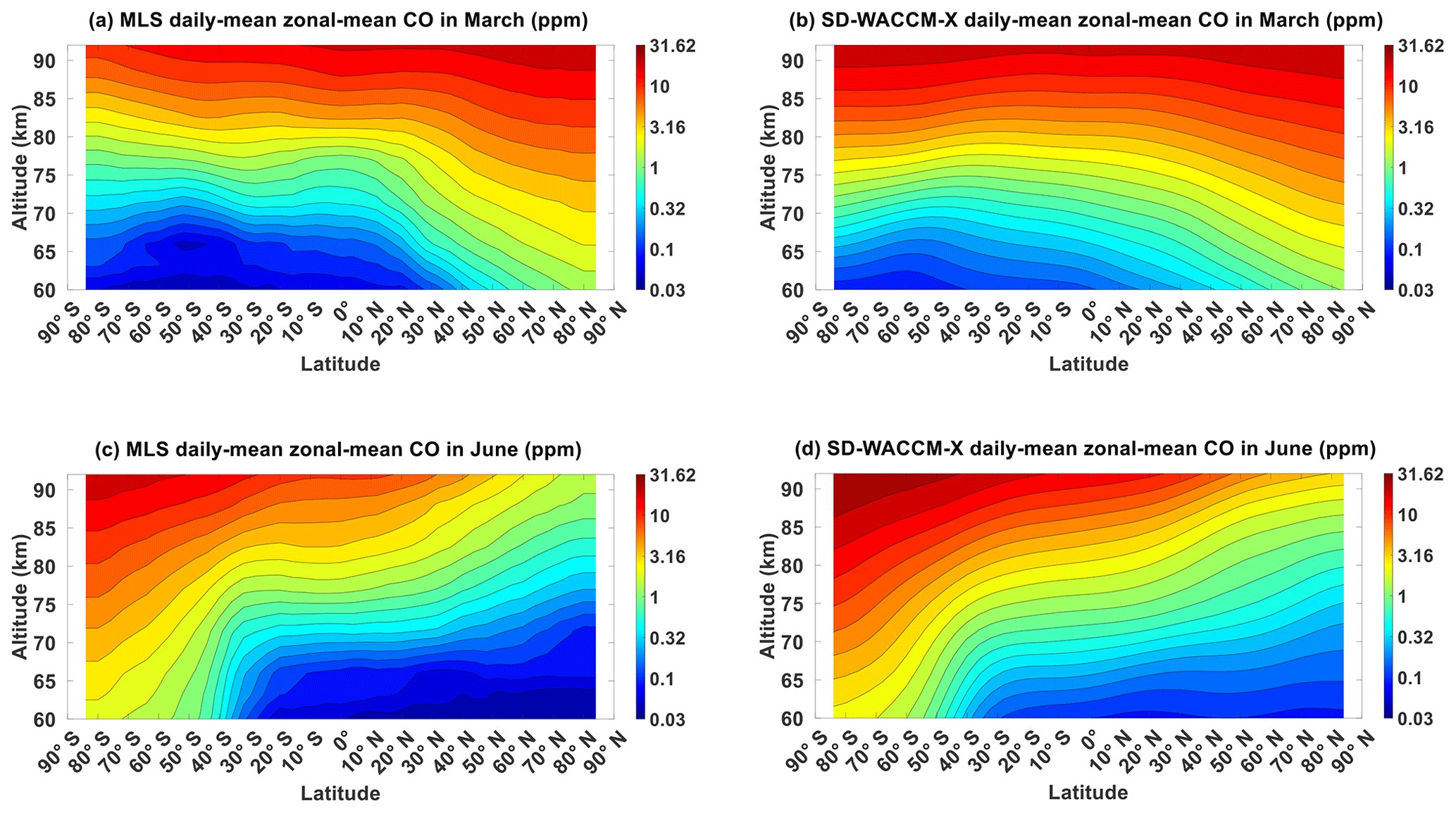
Figure 1Daily mean zonal-mean component of (a) MLS CO in March equinox, (b) SD-WACCM-X CO in March equinox, (c) MLS CO in June solstice and (d) SD-WACCM-X CO in June solstice. All are in units of ppm.
Figure 1 shows the CO averaged for all March equinox and for all June solstice as observed by MLS and as simulated by SD-WACCM-X. In both seasons and in both observations and models, CO shows interhemispheric asymmetry with larger asymmetry during solstice seasons than during equinox seasons (September equinox and December solstice shown in Fig. A1). The interhemispheric asymmetry is characterized by larger CO over the winter (during solstice months) and/or spring (during equinox months) hemispheres than the summer and/or fall hemispheres, respectively. The latitudinal gradient over the winter hemisphere maximizes during solstice seasons. These seasonal morphologies are known to be driven by the seasonality of the residual circulation (Garcia et al., 2014). While these seasonal morphologies are similar in both observations and models, there are still notable differences between them. During equinox seasons, MLS CO above 80 km is larger over the Equator than over the northern and southern low-latitudes. Below 80 km, MLS CO is lower over the Equator than over the northern and southern low-latitudes. This is not reproduced in the model. This may be attributed to the incomplete local-time sampling in MLS. With incomplete local-time sampling, the zonal-mean may have aliases from other tides, particularly the semidiurnal tides. During solstice seasons, the latitudinal (vertical gradient) gradient over the winter hemisphere is larger (weaker) in MLS CO than in SD-WACCM-X CO. This may be attributed to a weaker winter downwelling in the model than observed. These similarities and differences in MLS and SD-WACCM-X CO will be noted in the analyses that follow.
To determine potential issues related to the lack of full local-time sampling in MLS temperatures, this work utilizes temperature observations from the sounding of the atmosphere using broadband emission radiometry (SABER) instrument onboard the thermosphere ionosphere mesosphere energetics and dynamics satellite (Russell et al., 1999). This work specifically utilizes SABER v2.07 operational temperature profiles (Mertens et al., 2001, 2009; Kutepov et al., 2006; Garcia-Comas et al., 2008; Dawkins et al., 2018). Salinas et al. (2020) have pointed out that the assumption of no local-time variation in CO2 may be problematic above 90 km; however, this work focuses on altitudes below 92 km where the CO2 vertical gradient and thus local-time variations are negligible (Garcia et al., 2014). SABER has alternating latitudinal coverage of 82∘ N–53∘ S and 53∘ N–82∘ S that occur due to the spacecraft yaw cycle every ∼60 d. The mission has an orbital period of ∼1.6 h and a local-time precession of 12 min d−1. This orbit allows SABER to achieve full diurnal coverage after 60 d (Zhang et al., 2006). From these SABER temperature observations, we take all the profiles within 30 d before and after the 15th of every month, then bin them into a 30∘ longitude, 5∘ latitude, 2 km altitude and 3 h UT grid. We then use a 2D least-squares fit to calculate SABER temperatures' zonal-mean and DW1 component from these grids. From these DW1 amplitudes and phases, we reconstruct 02:00 LT and 14:00 LT zonal-mean temperature profiles. Finally, we apply the same process as done on the MLS 02:00 LT and 14:00 LT zonal-mean temperature profiles to calculate the SABER DW1 temperature components. However, we only show values between latitudes 50∘ S and 50∘ N because SABER's yaw cycle hinders full local-time coverage at higher latitudes.
In this section, we present the seasonality of CO μ′ and T′as observed by MLS and as simulated by SD-WACCM-X. To calculate the seasonality of MLS CO μ′ and T′, we first construct monthly mean 02:00 LT and 14:00 LT global zonal-mean profiles of CO and temperature. Each profile has a 4∘ latitude bin from latitude 84∘ S to latitude 84∘ N. We then calculate the composite seasonal average of these 02:00 LT and 14:00 LT zonal-mean profiles. Finally, we take the difference between the 02:00 LT and 14:00 LT zonal-mean profiles for each month. To calculate the seasonality of SD-WACCM-X CO μ′ and T′, we first calculate the monthly means of their longitude-latitude-pressure-UT profiles. Then, from these 4-dimensional profiles, a 2D least-squares fit is used to calculate their zonal-mean component as well as the DW1 amplitudes and phases. From these DW1 amplitudes and phases, we reconstruct their zonal-mean profiles at 02:00 LT and 14:00 LT local times. Finally, we apply the same process as done on the MLS 02:00 LT and 14:00 LT zonal profiles to calculate their DW1 components.
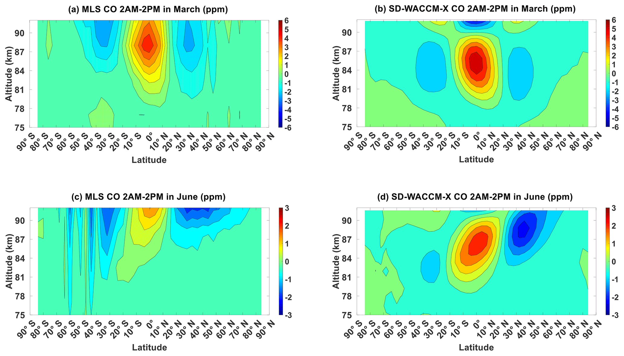
Figure 2Migrating diurnal tide component of (a) MLS CO in March equinox, (b) SD-WACCM-X CO in March equinox, (c) MLS CO in June solstice and (d) SD-WACCM-X CO in June solstice. All are in units of ppm.
Figure 2 shows CO μ′ in March equinox and in June solstice as observed by MLS and as simulated by SD-WACCM-X. For both equinox and solstice seasons, the largest MLS CO μ′ and SD-WACCM-X CO μ′ are found above 80 km (September equinox and December solstice shown in Fig. A2). When a dataset has full local-time coverage, Fig. 2 would come in the form of amplitude contour maps, and it would be accompanied by a phase contour map. The amplitude map will then clearly indicate where exactly the tides are strongest. In contrast, Fig. 2 and the other figures showing μ′ cannot indicate where exactly the tidal amplitudes are strongest. It can only indicate where the tide significantly affects CO (tidal perturbations), but it cannot indicate the relative strength of this influence.
Figure 2a shows that in March equinox, the largest MLS CO μ′ are above 80 km and have a latitude structure consistent with the (1,1) mode in temperature; that is, peak positive anomalies of around +6 ppm over the low-latitudes and peak negative anomalies of around −4 ppm over the mid-latitudes (Forbes, 1995; Mukhartov et al., 2009). The peak negative perturbation over the southern mid-latitudes begins at around 87 km and extends above 92 km, which is beyond MLS observation range. On the other hand, the peak negative perturbation over the northern mid-latitudes is located between 87 and 92 km. Figure 2b shows that in March equinox the largest SD-WACCM-X CO μ′ are also above 80 km and the latitude structure is also consistent with the (1,1) mode in temperature. However, unlike MLS, SD-WACCM-X CO μ′ exhibits two local maximum (hereafter referred to as “pulse”) of the (1,1) mode. The first pulse centered at around 87 km and the second pulse appears to be centered above 92 km. The pulses exhibit opposite phases of the (1,1) mode.
Figure 2c shows that in June solstice, the largest MLS CO μ′ perturbations begin at around 85 km and extend beyond 92 km. MLS CO μ′ has peak positive perturbations of around +2 ppm over the low-latitudes with higher values over the northern low-latitudes than over the southern low-latitudes. Over the Northern Hemisphere, MLS CO μ′ has peak negative perturbations of around −3 ppm extending from latitude 30∘ N to latitude 50∘ N. Over the Southern Hemisphere, the perturbations begin as negative perturbations of around −1 ppm extending from latitude 20∘ S to latitude 40∘ S. Then, it alternates between positive and negative perturbations from latitude 40∘ S to latitude 60∘ S. Ignoring the features poleward of latitude 40∘ S, the latitude structure of MLS CO μ′ in June solstice is consistent with the latitude structure of temperature's (1,1) mode “distorted” by the background atmosphere (Forbes, 1995; Mukhartov et al., 2009). By “distorted”, we hereafter mean the presence of other diurnal Hough modes.
Figure 2d shows that in June solstice SD-WACCM-X CO μ' also has a latitude structure consistent with a distorted (1,1) mode but unlike MLS, the model exhibits two pulses of the distorted (1,1) mode. The first pulse is centered at around 87 km and the second pulse is centered above 92 km. The pulses have opposite phases. In addition, SD-WACCM-X does not simulate the alternating positive and negative perturbations over the winter hemisphere. This could suggest that MLS observes mean-flow changes affecting these structures that are not simulated in the model.
Although the latitude structure of DW1 MLS CO μ′ and SD-WACCM-X CO μ′ have similarities to the DW1 temperature, it has never been proven that the DW1 tide affects CO. To establish this, we first characterize the DW1 component of temperature in the region and later use this to prove that the DW1 and (1,1) tide affects CO.
Figure 3 shows T′ in March equinox and in June solstice as observed by MLS and by SABER and as simulated by SD-WACCM-X (September equinox and December solstice shown in Fig. A3). Since we are focused on relating this to CO μ′, we focus on features above 80 km where CO μ′ is largest for both seasons. Figure 3a shows that in March equinox, MLS T′ has very similar latitude structure to MLS CO μ′; that is, it is consistent with the (1,1) mode. Figure 3c shows SABER T′ also in March equinox. SABER T′ has peak positive perturbations of around 30 K over the Equator which are larger than MLS T′'s. This difference may be attributed to aliasing of other tides on MLS T′ particularly the migrating semidiurnal tides. It may also be attributed to differences in the instruments' vertical resolutions. SABER has a vertical resolution of ∼2 km while MLS has a vertical resolution of ∼10 km (Remsberg et al., 2008; Livesey et al., 2011). Given that DW1 typically has a vertical wavelength of ∼ 25–30 km, MLS's coarser vertical resolution can substantially reduce the amplitudes. SABER T′'s peak negative perturbations over the northern and southern mid-latitudes are both found between 80 and 90 km unlike MLS T′. This difference may also be attributed to the uneven sampling of MLS over the middle to high latitudes and/or the vertical resolution differences. Both MLS T′ and SABER T′ exhibit features consistent with the (1,1) mode although there are clear differences in terms of their structure's hemispheric symmetry (Forbes, 1995; Mukhartov et al., 2009). MLS T′'s (1,1) mode appears tilted upward because its southern mid-latitude peak appears higher than its northern mid-latitude peak. SABER T′'s (1,1) mode's mid-latitude peaks occur in almost the same altitude, but the northern mid-latitude amplitudes are larger than the southern mid-latitude amplitudes. Figure 3e shows that in March equinox SD-WACCM-X T′ has a latitude structure very similar to that of SD-WACCM-X CO μ′.
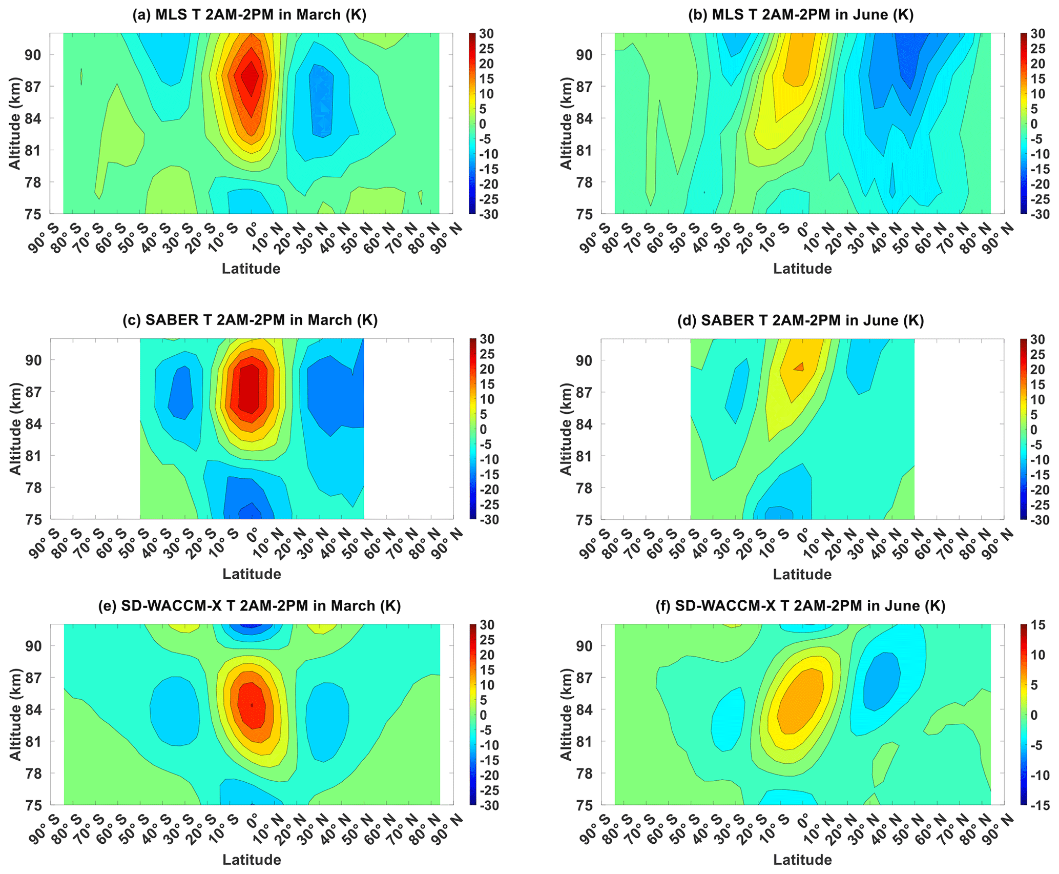
Figure 3Migrating diurnal tide component of (a) MLS temperature in March equinox, (b) MLS temperature in June solstice, (c) SABER temperature in March equinox, (d) SABER temperature in June solstice, (e) SD-WACCM-X temperature in March equinox and (f) SD-WACCM-X temperature in June solstice. All are in units of K.
In March equinox, MLS T′ and SABER T′ observe only one pulse of the (1,1) mode between 80 and 92 km while SD-WACCM-X T′ simulates almost two pulses. This may be attributed to the model inaccurately simulating DW1's altitudinal variations. On the other hand, MLS T′ and SABER T′ are different over the mid-latitudes. This shows that the differences between MLS T′ and SABER T′ over the mid-latitudes may also be attributed to aliasing of the migrating semidiurnal tide into MLS T′.
Figure 3b shows that in June solstice MLS T′ exhibits a latitude structure consistent with the distorted (1,1) mode (Forbes, 1995; McLandress, 1997; Mukhartov et al., 2009). It is very similar with MLS CO μ′. One major difference is that the largest values in MLS CO μ′ are above 85 km. Figure 3d shows SABER T′ also in June solstice. SABER T′ also exhibits features consistent with the distorted (1,1) mode. These differences between MLS T′ and SABER T′ over the mid-latitudes may be a result of MLS inadequate sampling causing significant aliasing from other tides. Our approach in calculating the DW1 component with MLS is susceptible to aliasing from the migrating semidiurnal tide (Oberheide et al., 2003). In solstice, the migrating semidiurnal tide is known to be significant over the winter mid-latitudes (Zhang et al., 2006). These may all contribute to the aliasing in MLS T′. Like MLS T′, these features are also consistent with the presence of a distorted (1,1) mode. Figure 3f shows that in June solstice, unlike MLS T′ and SABER T′, SD-WACCM-X T′ shows two pulses of the distorted (1,1) mode above 80 km. In June solstice, MLS T′ and SABER T′ observe only one pulse of the distorted (1,1) mode between 80 km and 92 km while SD-WACCM-X T′ simulates almost two pulses. This is like the case in March equinox. This indicates that the model's inaccuracies in simulating DW1's altitudinal variations occur in all seasons.
Figures 2 and 3 clearly show that the latitude–altitude structure of CO μ′ and T′ are remarkably similar when looking at either MLS observations or SD-WACCM-X simulations. Since the latitude–altitude structure of observed or simulated T′ is already known to be predominantly driven by DW1, Figs. 2 and 3 suggest that the latitude–altitude structure of CO μ′ may also be driven by DW1. However, the mechanisms of how DW1 can affect CO μ′ have never been determined. In this section, we present the physical mechanisms of how DW1 affects CO. This section is divided into two subsections. One subsection is about the physical mechanisms during March equinox, while the other subsection is about the mechanisms during June solstice.
5.1 March equinox CO DW1
To determine the physical mechanisms, we took a two-step approach. Step 1 is a tendency analysis involving the continuity equation for a tracer given by (Brasseur and Solomon, 2006)
where μ is CO volume mixing ratio, t is time, ϕ is latitude, λ is longitude and z is geopotential height. The variables u, v and w are the neutral zonal, meridional and vertical winds, respectively; Kzz is the eddy diffusion coefficient; Dμ is the molecular diffusion coefficient and wD is its corresponding diffusive separation velocity; P is the chemical production rate; L is the chemical loss rate; ρ0 is the atmospheric neutral density; and a is the radius of the Earth which is 6.37×10⁶ m. Note that the eddy diffusion coefficient is calculated from a gravity wave parameterization (Richter et al., 2010; Garcia et al., 2017). The molecular diffusion coefficient is as defined in Smith et al. (2011). The DW1 component of each term is calculated by fitting the terms into the equation using a 2D least-squares fit. This determines the contributions of zonal advection, meridional advection, vertical advection, eddy diffusion, molecular diffusion and photochemical production to SD-WACCM-X CO μ′'s DW1 component. Comparing these terms will determine the main processes behind SD-WACCM-X CO μ′. Salinas et al. (2020) recently used this to determine the mechanisms of lower thermospheric carbon dioxide's (CO2) local-time variations. The result of this analysis gives us SD-WACCM-X's suggested mechanisms for μ′. This first method is clearly only applicable with model outputs because some of the required parameters cannot currently be observed.
Figures 4a, b and B1 show the results of our tendency analysis for March equinox season. Figure 4a shows the DW1 amplitude of the time-derivative term in the continuity equation. It can be characterized by a primary equatorial peak of around 30 ppm d−1 between 85 and 92 km as well as secondary mid-latitude peaks of around 12 ppm d−1 between similar altitudes. This latitude structure is consistent with that of the (1,1) mode. Figure 4b shows the DW1 amplitude of the vertical advection term in the continuity equation. It exhibits a similar magnitude and latitude–altitude profile to Fig. 4a. Figure B1 shows the DW1 amplitudes of the other terms in the continuity equation. These figures show that in SD-WACCM-X, vertical advection in March equinox has the closest magnitude and latitude–altitude structure to the time-derivative term. Chemical production has a higher magnitude than vertical advection but because, as mentioned earlier, the chemical production timescale is slower than dynamical timescales, its latitude–altitude structure is not similar to the time-derivative term.
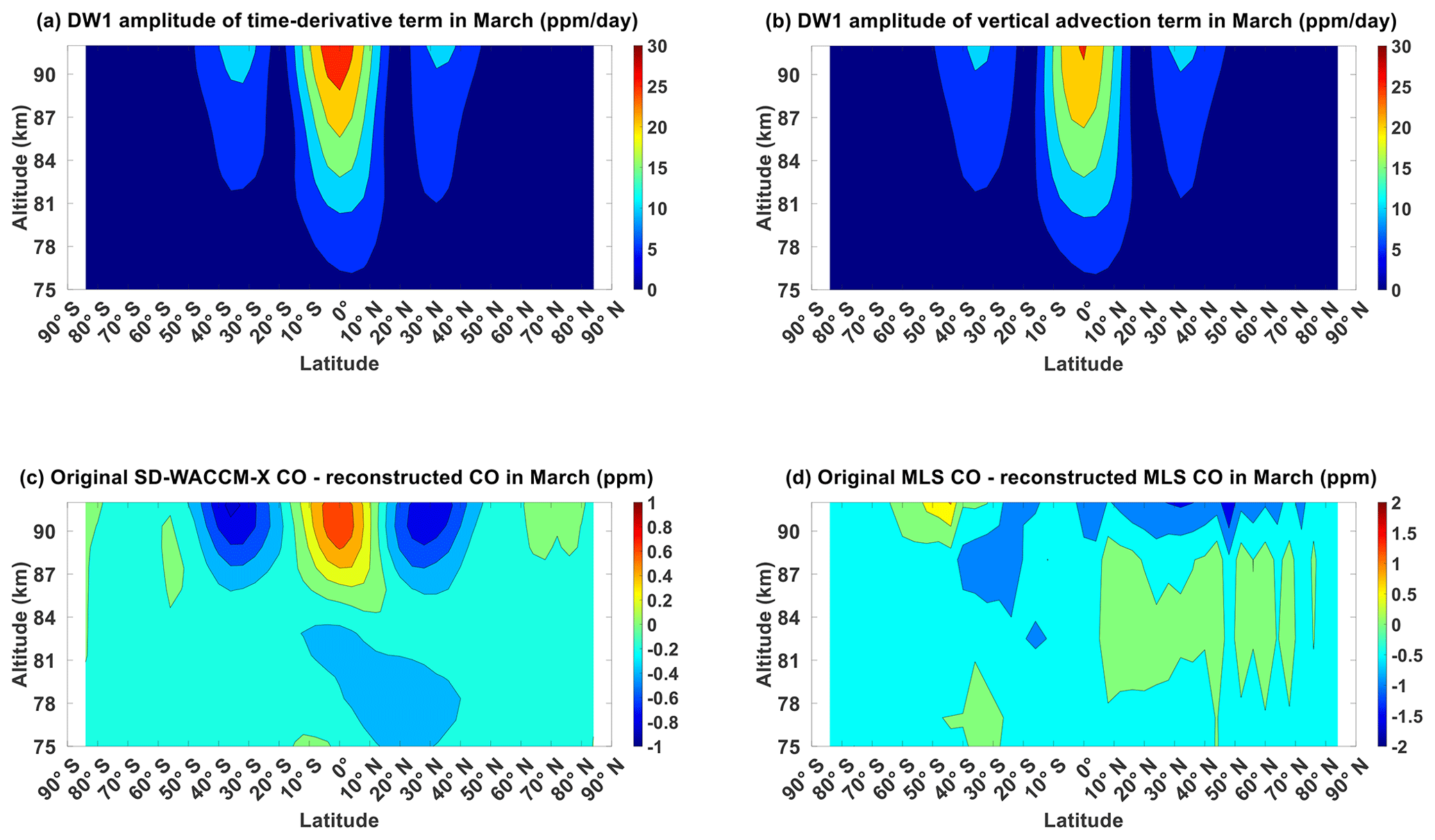
Figure 4Migrating diurnal tide component in March equinox of (a) CO's time-derivative term and (b) CO's vertical advection term. (c) Difference between SD-WACCM-X CO's DW1 component and SD-WACCM-X CO's DW1 component reconstructed using adiabatic displacement method. (d) Difference between MLS CO's DW1 component and MLS CO's DW1 component reconstructed using adiabatic displacement method. Units are specified in the plots.
Now, we need to determine if the same mechanism holds for the observations. This is step 2. A tendency analysis is still currently impossible with observations because we do not have observations of all the needed parameters. However, we can use a method called the adiabatic displacement method to quantify the contributions of vertical advection on CO μ′ as observed by MLS and as simulated by SD-WACCM-X. The adiabatic displacement method involves calculating the perturbation on a tracer due to any tide-induced vertical advection using the following equation:
T′ is the tidal perturbation of temperature. is static stability. g is the acceleration due to gravity (9.8 m s−2). cp is the heat capacity of air at constant pressure (1004 JK−1 kg). is the vertical gradient of a tracer's zonal-mean profile. This equation is derived by first linearizing the continuity equation (Eq. 2). Then, we assume only the vertical advection term is important. Finally, we set all primed variables into the form ei(kx−σt), where k is the zonal wave number and σ is the tidal frequency. This gives us the following equation:
The same can be done to a form of the thermodynamic equation that assumes all temperature changes are due to adiabatic motion. This gives us the following equation:
Combining Eqs. (4) and (5) gives Eq. (3).
Comparing CO μ′ and CO will determine how much of CO μ′ is driven by vertical advection. If CO μ′ and CO μw′ are similar, then we can argue that vertical advection does primarily drive CO μ′. Applying this method on the model outputs will assess the consistency of this method and the previous method with regards the role of vertical advection in μ′. Forms of this method have already been applied on the analysis of the tidal or local-time variations of other tracers (Akmaev et al., 1980; Angelats I Coll and Forbes, 1998; Marsh et al., 1999; Shepherd et al., 1995, 1997; Ward, 1999; Zhang et al., 1998; Marsh and Russell, 2000; Oberheide and Forbes, 2008; Smith et al., 2010; Marsh et al., 2011; Salinas et al., 2022)
Apart from proving that vertical advection primarily drives CO μ′, Eq. (3) will also explain why the latitude and altitude structure of a tracer's DW1 component and temperature's DW1 component may be correlated. Equation (3) indicates that if vertical advection does primarily drive a tracer's DW1 component, and since Fig. 1 has shown that zonal-mean CO's vertical gradient is positive, CO μ′ and T′ are correlated. This also indicates that an increase in μ' requires T′>0, which under adiabatic conditions implies a net downwelling. Conversely, a decrease in μ′ implies T<0′ and net adiabatic upwelling.
Figure 4c shows the differences between SD-WACCM-X CO μ′ and SD-WACCM-X CO μw′. The differences are within ±0.6 ppm. Peak positive difference of around +0.6 ppm is found over the Equator, while peak negative difference of around −0.6 ppm is found over the mid-latitudes. These differences are an order of magnitude lower from the correct values which indicates that SD-WACCM-X CO μw′ is very similar to SD-WACCM-X CO μ′. Thus, Fig. 4a, b and c indicate that in the model, CO μ′ and CO μw′ are very similar in March equinox. This explains the positive correlation between the latitude structure of SD-WACCM-X CO μ′ and SD-WACCM-X T′ in March equinox. We now show MLS CO in Fig. 4d. Figure 4d shows that the largest differences are above 90 km. Below 90 km, the average difference is around −0.5 ppm. This also indicates good similarity in March equinox between MLS CO μ′ and MLS CO μw′. This explains the positive correlation between the latitude structure of MLS CO μ′ and MLS T′ in March equinox. For both MLS CO μ′ and SD-WACCM-X CO μ′, Fig. 4c and d indicate that the positive perturbations are driven by a relative downwelling due to the DW1 tide, while the negative perturbations are driven by a relative upwelling.
5.2 June solstice CO DW1
We now determine the physical mechanisms behind CO μ′ in June solstice. We first show the results of the tendency analysis in SD-WACCM-X. Figure 5a shows the DW1 amplitude of the time-derivative term in the continuity equation. It can be characterized by a primary low-latitude peak of around 8–12 ppm d−1 between 85 and 95 km. Amplitudes are larger over the northern low-latitude than over the southern low-latitude. Mid-latitude peaks are also present, but the northern mid-latitude peak of around 7 ppm d−1 is larger than the southern mid-latitude peak of around 3 ppm d−1. Figure 5b shows the DW1 amplitude of the vertical advection term in the continuity equation. It shows a similar magnitude and latitude–altitude profile to Fig. 5a. Figure B2 shows the DW1 amplitudes of the other terms in the continuity equation. These figures show that in SD-WACCM-X, vertical advection in June solstice has the closest magnitude and latitude–altitude structure to the time-derivative term. Like March equinox, the chemical production also has a higher magnitude than vertical advection, but its latitude–altitude structure also is not similar with the time-derivative term.
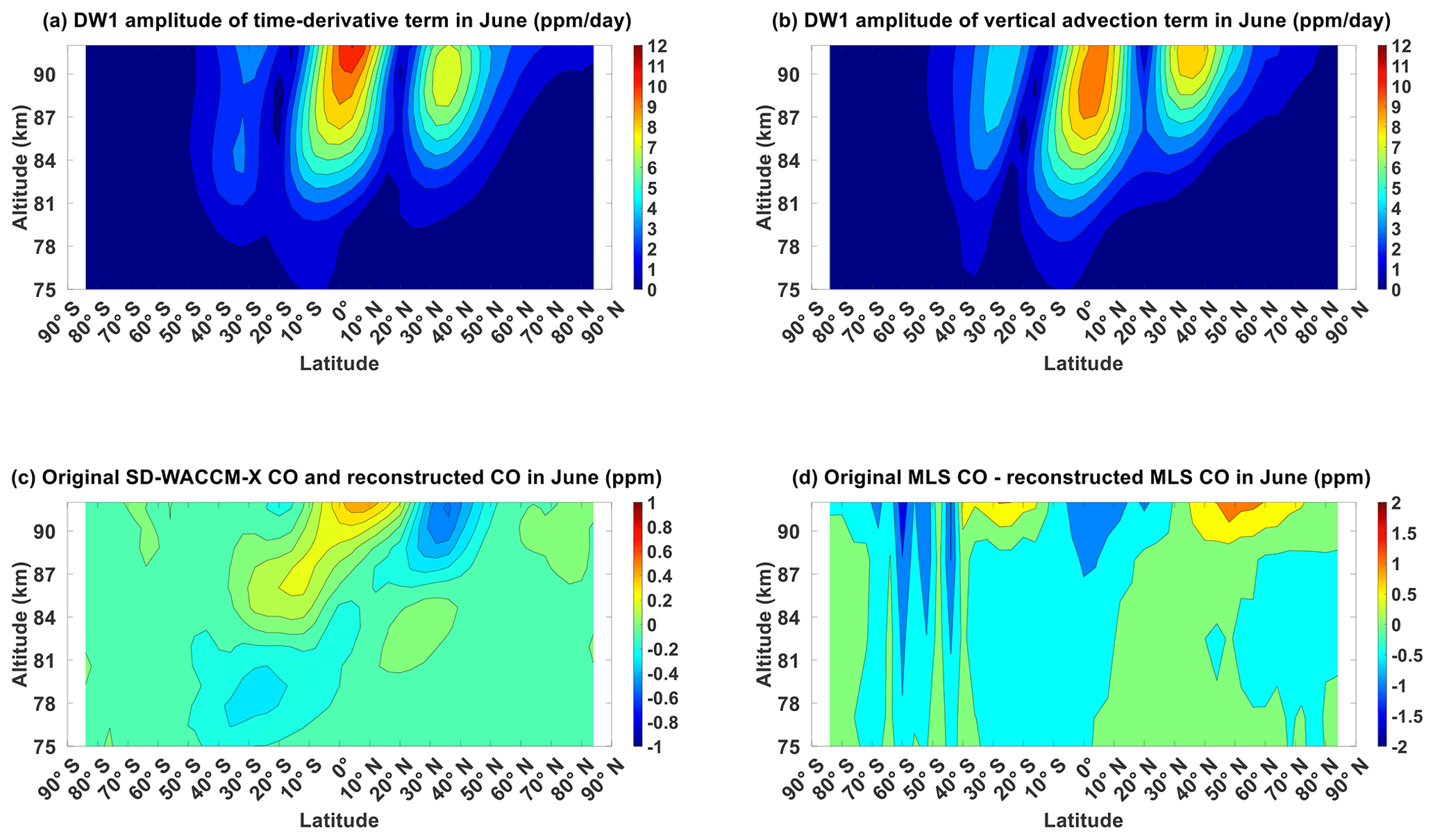
We now also use the adiabatic displacement method to quantify how much CO changes due to DW1-induced vertical advection in June solstice. Figure 5c shows the differences between SD-WACCM-X CO μ′ and SD-WACCM-X CO μw′ for June solstice. The differences are within ±0.5 ppm. Peak positive difference of around +0.5 ppm is found over the Equator above 90 km, while peak negative difference of around −0.4 ppm is found over the northern mid-latitudes. These differences are also an order of magnitude lower than the correct values, which indicates that SD-WACCM-X CO μw′ is very similar to SD-WACCM-X CO μ′. Thus, Fig. 5a, b and c indicate that in the model CO μ′ and CO μw′ are remarkably similar in June solstice. These figures indicate that for SD-WACCM-X in June solstice the positive perturbations are driven by a relative downwelling due to the DW1 tide, while the negative perturbations are driven by a relative upwelling.
We now show June solstice MLS CO in Fig. 5d. Figure 5d shows that the largest differences between latitudes 30∘ S and 60∘ N are above 90 km. Below 90 km, the average difference is around −0.5 ppm. This also indicates good similarity between MLS CO μ′ and MLS CO μw′ in June solstice for regions less than 90 km between latitudes 30∘ S and 60∘ N. On the other hand, between latitudes 30 and 60∘ S, the largest differences are found between 80 and 92 km. This also indicates that, unlike in March equinox, MLS CO μ′ and MLS CO μw′ are not similar throughout all latitudes in June solstice. They are only similar between latitudes 30∘ S and 60∘ N. These figures indicate that for MLS in June solstice not all positive perturbations are driven by a relative downwelling, and not all negative perturbations are driven by a relative upwelling.
The previous sections have shown that for both observations and simulations CO μ′ is predominantly very similar to CO μw′. It is also shown that CO μ′'s latitude–altitude structure appears to be predominantly comprised of the (1,1) mode. In this section, we now focus on determining vertical advection's impact on the seasonal and interannual variabilities of CO's (1,1) mode. To calculate the (1,1) mode of CO μ′ (hereafter referred to as CO hμ′), we project the latitude profiles at each altitude in CO μ′ with the (1,1) Hough mode profile (Forbes, 1995).
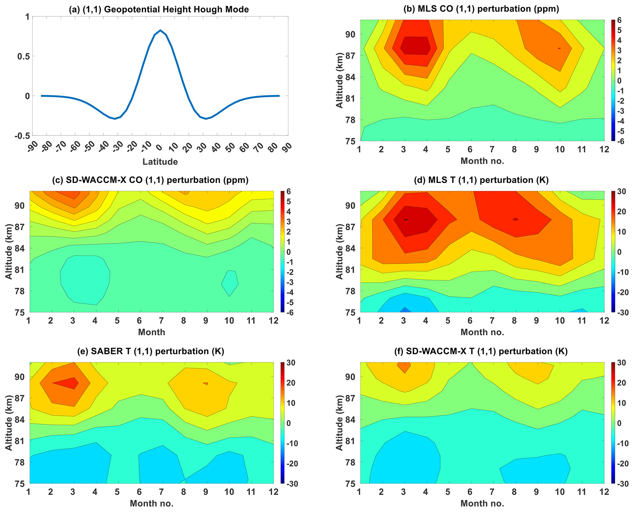
Figure 6(a) (1,1) Hough mode for geopotential height. Seasonality of the (1,1) component of (b) MLS CO, (c) SD-WACCM-X CO, (d) MLS temperature, (e) SABER temperature and (f) SD-WACCM-X temperature. Units are specified in the plots.
6.1 (1,1) Hough mode component's seasonality
This subsection will determine the seasonal and interannual variability of the (1,1) mode of CO. To explain it, we will first compare the (1,1) mode of CO with the (1,1) mode of temperature (hT′). Then, we will determine the role of vertical advection by projecting the latitude profiles at each altitude of CO μw′ (presented in Sect. 5) with the (1,1) Hough function profile. The corresponding projection coefficients will be denoted as CO hw′.
Figure 6 first shows the seasonality of observed and modeled CO hμ′ and hT′. Figure 6a shows the (1,1) mode. Figure 6b shows the seasonality of MLS CO hμ′. The largest coefficients are above 80 km, and they are all positive projection coefficients, indicating that there is a positive correlation between a latitude profile of MLS CO μ′ and the (1,1) Hough mode between 80 and 92 km. This is consistent with the features shown in Fig. 2a and c. Between 80 and 90 km, the seasonality is characterized by a semi-annual oscillation with primary peak of around 4 ppm in March equinox and secondary peak of around 3 ppm in September equinox. Above 90 km, it appears as though the primary peak is moving towards June solstice. Figure 6c shows the seasonality of SD-WACCM-X CO hμ′. The largest coefficients are above 85 km, and they are all also positive projection coefficients. Between 85 and 95 km, the seasonality is also characterized by a semi-annual oscillation with primary peak of around 6 ppm in March equinox and secondary peak of around 5 ppm in September equinox. Figure 6b and c shows that SD-WACCM-X does capture the observed semi-annual oscillation of the projection coefficients. However, the altitudinal variations are different from observed. This is consistent with the differences in MLS CO μ′ and SD-WACCM-X CO μ′. The coefficients of SD-WACCM-X CO hμ′ are also higher than MLS.
Figure 6d shows the seasonality of MLS hT′. Focusing on the coefficients above 80 km, we find that, like MLS CO, they are all positive projection coefficients, indicating that there is a positive correlation between MLS T′ and the (1,1) Hough mode between 80 and 92 km. Between 80 and 90 km, it also has a semi-annual oscillation with primary peak coefficients of around 25 K during March equinox and secondary peak coefficients of around 20 K during September equinox. Above 90 km, the seasonality appears to shift into an annual oscillation with peak amplitudes in June solstice. Figure 6e shows the seasonality of SABER hT′. Between 80 and 95 km, it also has a semi-annual oscillation with primary peak of around 20 K during March equinox and secondary peak of around 15 K during September equinox. Unlike MLS hT′, its seasonality does not seem to change above 90 km. Figure 6f shows the seasonality of SD-WACCM-X hT′. Between 80 and 95 km, it also has a semi-annual oscillation with primary peak of around 27 K during March equinox and secondary peak of around 20 K during September equinox. Unlike MLS hT′, its seasonality does not also seem to change above 90 km. Also, SD-WACCM-X hT′ is consistently larger than SABER hT′, but its coefficients are not too different from MLS hT′.
Figure 6b and d showed that the seasonality of MLS CO hμ′ and MLS hT′ is similar. However, MLS hT′ and SABER hT′ in Fig. 6e have differences. The seasonality of MLS hT′ changes slightly above 90 km, while the seasonality of SABER hT′ does not. Figure 6b, d and e shows that the seasonality of MLS CO hμ′ may be affected by the incomplete local-time sampling of MLS or its coarse vertical resolution. This would be consistent with the results shown in Figs. 2 and 3. Figures 2 and 3 showed that MLS CO μ′ and MLS T′ may be affected by inadequate sampling over the mid-latitudes.
Figure 6b and c showed that MLS CO hμ′ is stronger than SD-WACCM-X CO hμ′. Figure 6e and f also showed that SABER hT′ is stronger than SD-WACCM-X hT′. A larger MLS CO hμ′ than simulated is consistent with a larger realistic MLS or SABER hT′ than simulated. An underestimation of SD-WACCM-X hT′ indicates inaccuracies in the simulated background atmosphere, tidal source or tidal dissipation mechanisms.
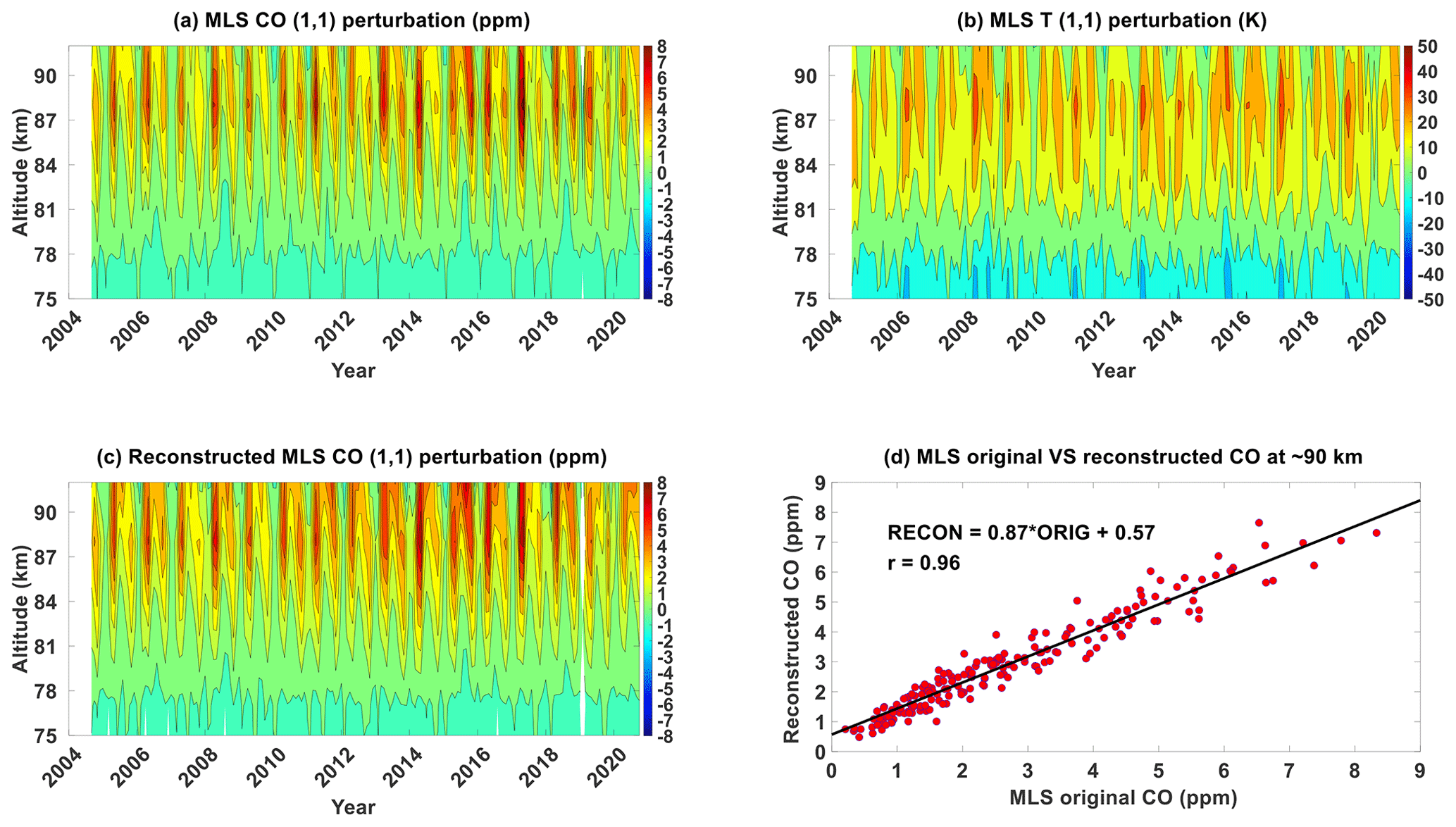
Figure 7(1,1) component of (a) MLS CO, (b) MLS temperature and (c) MLS CO reconstructed using the adiabatic displacement method from 2004 until 2021. (d) Scatter plot between MLS CO's (1,1) component at ∼90 km and that is reconstructed using the adiabatic displacement method. Units are specified in the plots.
6.2 Role of vertical advection on the CO (1,1) mode across interannual timescales
Apart from these differences amongst the datasets, Fig. 6b and d as well as Fig. 6c and f shows that CO hμ′ and hT′ in MLS observations and SD-WACCM-X simulations have similarities in their seasonality. We now check whether this similarity is also found for all months and all years of MLS observations and SD-WACCM-X simulations. We will also check if CO hμ′ is primarily driven by vertical advection across all months and years of observations and simulations. In this subsection, we determine the importance of vertical advection by projecting the latitude profiles at each altitude of the previously calculated CO μw′ with the (1,1) Hough function profile. The corresponding projection coefficients will be denoted as CO hw′.
Figure 7a shows the MLS CO hμ′ from 2004 until 2020. Figure 7b shows MLS CO hT′ from 2004 until 2020. Their overall morphology is similar; that is, for all years, there is a semi-annual oscillation with primary peak in March equinox and secondary peak in September equinox between 80 km and 90 km. Above 90 km, their seasonality shifts into having a primary peak close to June solstice. This could suggest that the latitude structure of DW1's phase during solstice (equinox) causes maximum (minimum) values when taking the difference of values at ∼ 02:00 LT and at ∼ 14:00 LT. This consequently enhances (reduces) MLS CO hμ′. This is difficult to validate, with a very high degree of uncertainty even with SABER data, because of the differences in MLS and SABER's vertical resolution. Figure 7c shows the MLS CO hw′. Comparing Fig. 7a and c shows that most of the seasonal features are indeed captured. Figure 7d shows a scatter plot between CO hμ′ and CO hw′ at ∼90 km, which is the approximate altitude where these MLS parameters attain peak amplitudes. It shows a correlation of 0.97, indicating that the variations of hμ′ and hw′ are very similar.
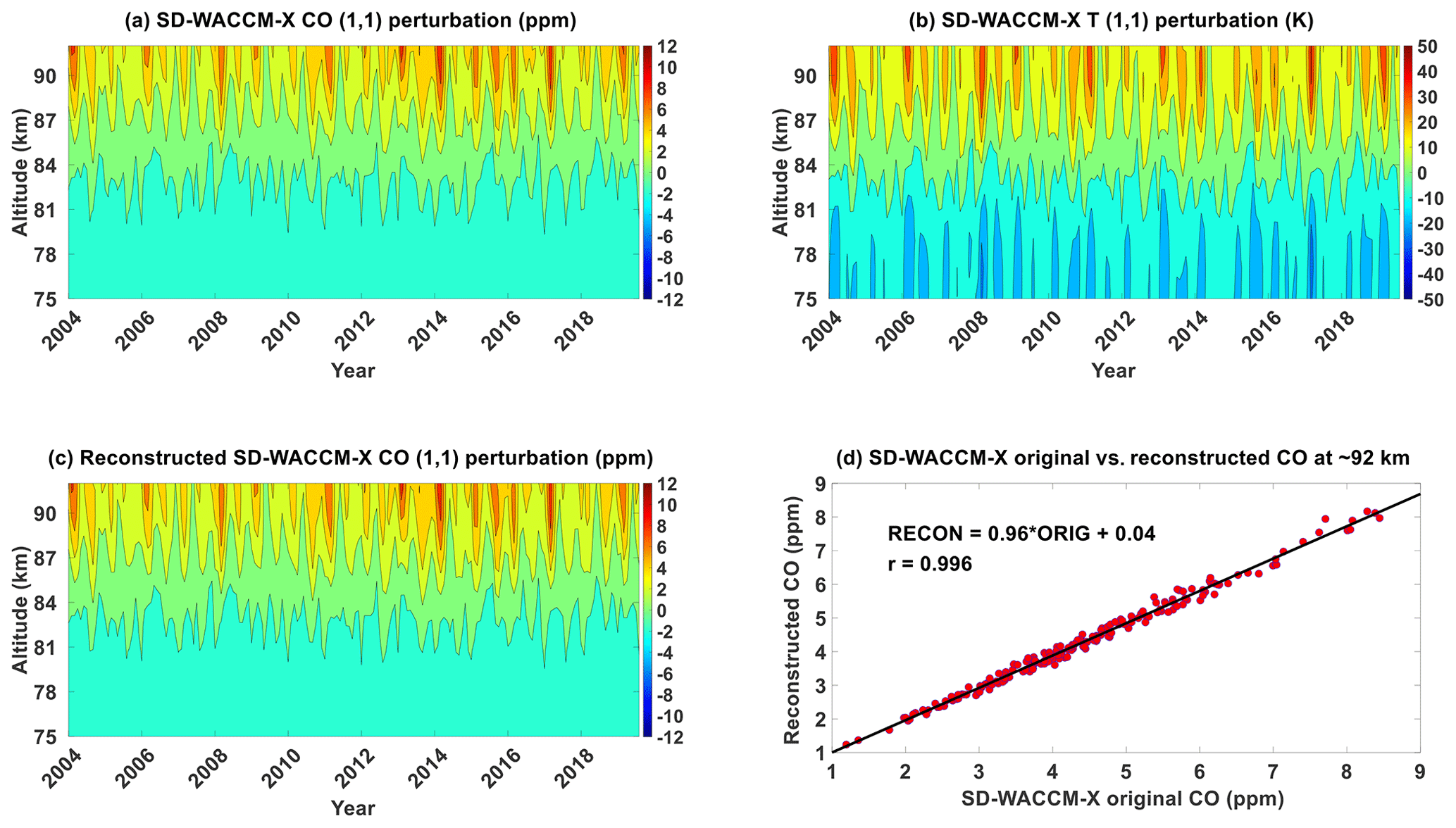
Figure 8(1,1) component of (a) SD-WACCM-X CO, (b) SD-WACCM-X temperature and (c) SD-WACCM-X CO reconstructed using the adiabatic displacement method from 2004 until 2021. (d) Scatter plot between SD-WACCM-X CO's (1,1) component at ∼92 km and that is reconstructed using the adiabatic displacement method. Units are specified in the plots.
Figure 8a shows SD-WACCM-X CO hμ′ from 2004 until 2020. Figure 8b shows SD-WACCM-X hT′ from 2004 until 2020. Their overall morphology is also similar; that is, for all years, there is a semi-annual oscillation with primary peak in March equinox and secondary peak in September equinox. We now calculate SD-WACCM-X CO hw′. Figure 8c shows the SD-WACCM-X CO hw′. Comparing Fig. 8a and c shows that most of the features are indeed captured. Figure 8d shows a scatter plot between SD-WACCM-X CO hμ′ and SD-WACCM-X CO hw′ at ∼92 km, which is the approximate altitude where these SD-WACCM-X parameters reach peak amplitudes. It shows a correlation of 0.996, indicating that the variations of CO hμ′ and CO hw′ are very similar. This correlation is higher than MLS CO hμ′. We suggest that this may be due to the aliasing over the mid-latitudes in MLS CO μ′ Previous studies using this adiabatic displacement method only involved the analysis of tracer observations at one instance in time (Akmaev et al., 1980; Angelats I Coll and Forbes, 1998; Marsh et al., 1999; Shepherd et al., 1995, 1997; Ward, 1999; Zhang et al., 1998; Marsh and Russell, 2000; Oberheide and Forbes, 2008; Smith et al., 2010; Marsh et al., 2011; Salinas et al., 2020, 2022). Our work adds to these studies by presenting an approach involving the adiabatic displacement method that involves proving the importance of vertical advection at both seasonal and interannual timescales.
6.3 Cross-wavelet analysis
Figures 7 and 8 indicate that, across interannual timescales, both observed and modeled CO hμ′ and CO hw′ are highly correlated. In this subsection, we identify the interannual phenomena in CO hμ′ that can apparently also be seen in CO hw′ because they are both highly correlated. We focus on interannual phenomena that are known to already affect the (1,1) mode in temperature: the quasi-biennial oscillation and the El Niño–Southern Oscillation (Lieberman, 1997; Vincent et al., 1998; McLandress, 2002a, b; Gurubaran et al., 2005, 2009; Mayr and Mengel, 2005; Liebermann et al., 2007; Wu et al., 2008; Mukhtarov et al., 2009; Pancheva et al., 2009; Xu et al., 2009; Pedatella et al., 2012, 2013; Gan et al., 2014; Liu et al., 2017; Zhou et al., 2018; Kogure et al., 2021; Pramitha et al., 2021; Cen et al., 2022). We use a cross-wavelet analysis to determine the dominant oscillations in MLS CO hμ′ or SD-WACCM-X CO hμ′ that coincide with the 30 mb QBO index and multi-variate El Niño–Southern Oscillation index (MEI).

Figure 9(a) De-seasonalized time-series of MLS CO (1,1) at ∼90 km, SD-WACCM-X CO (1,1) at ∼92 km and the QBO index. (b) De-seasonalized time-series of MLS CO (1,1) at ∼90 km, SD-WACCM-X CO (1,1) at ∼92 km and the ENSO index. (c) Cross-wavelet (XWT) spectrum between MLS CO (1,1) at ∼90 km and the QBO index. (d) Cross-wavelet spectrum between MLS CO (1,1) at ∼90 km and the ENSO index. (e) Cross-wavelet spectrum between SD-WACCM-X CO (1,1) at ∼92 km and the QBO index. (f) Cross-wavelet spectrum between SD-WACCM-X CO (1,1) at ∼92 km and the ENSO index.
Figure 9 identifies interannual phenomena found in CO hμ′. Figure 9a shows the time-series of MLS CO hμ′ at ∼90 km, SD-WACCM-X CO hμ′ at ∼92 km and the QBO index. Figure 9b shows the time-series of MLS CO hμ′ at ∼90 km, SD-WACCM-X CO hμ′ at ∼92 km and the MEI index. Figure 9c shows the cross-wavelet spectrum between MLS CO hμ′ and the QBO index. In this and the succeeding spectra, encircled regions with the high spectral power correspond to oscillations statistically significant in both time-series (Grinsted et al., 2004). The arrows indicate the phase relationship between the time-series. If the arrow points right, both time-series are in phase. If the arrow points left, both time-series are anti-phase. If the arrow points upward or downward, there is a lag between the time-series. In our case, an upward arrow indicates that both time-series are in phase but the QBO or ENSO index time-series peaks later than the other time-series. A downward arrow indicates that both time-series are also in phase but the QBO or ENSO index time-series peaks ahead of the other time-series. Depending on the arrows, one can deduce the correlations between CO hμ′ amplitude and QBO or ENSO. Consequently, the deduced correlation will imply whether CO hμ′ increases or decreases during, for example, westerly QBO phase.
Figure 9c reveals that both MLS CO hμ′and the QBO index have a statistically significant oscillation with periods of around 24 months. It is statistically significant between 2005 and 2018. The arrows are pointed slightly upward which indicates that MLS CO hμ′ peak slightly ahead of the QBO index. The arrows also indicate that MLS CO hμ′ amplitude increases during the westerly phase of the QBO while it decreases during the easterly phase of the QBO. Remarkably similar features are found in the cross-spectrum between MLS hT′ and the QBO index (Fig. C1c). The QBO's impacts on the (1,1) mode of temperature is well known (Lieberman, 1997; Vincent et al., 1998; Mayr and Mengel, 2005; Wu et al., 2008; Gurubaran et al., 2009; Mukhtarov et al., 2009; Pancheva et al., 2009; Xu et al., 2009; Gan et al., 2014; Pramitha et al., 2021). These studies have shown that the (1,1) mode is enhanced during the westerly phase of the QBO while it is reduced during the easterly phase of the QBO. Our work adds to these previous studies by showing that MLS CO's (1,1) mode is also affected by the QBO in the same way.
Figure 9d shows the cross-wavelet spectrum between MLS CO hμ ′and the MEI index. This spectrum reveals that both MLS CO hμ′ and the MEI index have a statistically significant oscillation of around 30 months between 2008 and 2012. This does coincide with the strong 2010–2011 La Niña event. The arrows are pointed almost fully to the left, which indicates that MLS CO hμ′ and ENSO are anti-correlated during this event; that is, MLS CO hμ′ amplitude increased during this La Niña event. The anti-correlation also indicates that, if we were to solely use this event as a basis, MLS CO hμ′ should decrease during El Niño events. Very similar features are found in the cross-spectrum between MLS hT′ and the ENSO index (Fig. C1d). ENSO's impacts on the (1,1) mode of tide is well explored (Gurubaran et al., 2005; Liebermann et al., 2007; Pedatella et al., 2012, 2013; Liu et al., 2017; Zhou et al., 2018; Kogure et al., 2021; Cen et al., 2022). These studies have shown that the general response is that (1,1) mode is reduced during El Niño, although the reduction is modulated by secondary mechanisms like gravity waves (Cen et al., 2022).
Figure 9e shows the cross-wavelet spectrum between SD-WACCM-X CO hμ′ and the QBO index. This spectrum reveals that both SD-WACCM-X CO hμ′ and the QBO index have a statistically significant oscillation with periods ranging from 20 to 30 months, and the statistical significance is found throughout all years. From 2015 to 2020, both have a statistically significant oscillation with a period of around 15 to 20 months. Very similar features are found in the cross-spectrum between SD-WACCM-X hT′ and the QBO index (Fig. C1e). Like MLS CO hμ′, the arrows are pointed slightly upward, which indicates that SD-WACCM-X CO hμ′ peaks slightly ahead of the QBO index and that SD-WACCM-X CO hμ′ amplitude increases during the westerly phase of the QBO while it decreases during the easterly phase of the QBO. The differences between Fig. 9c and e could suggest that the model may be overestimating the impacts of the QBO during certain periods.
Figure 9f shows the cross-wavelet spectrum between SD-WACCM-X CO hμ′ and the MEI index. This spectrum reveals that both have a statistically significant oscillation with a period of around 24 to 36 months. This period of statistical significance lasts from 2006 to 2016. Unlike MLS CO hμ′, the statistical significance for SD-WACCM-X CO hμ′ includes both the 2010–2011 La Niña and the 2015–2016 El Niño event. The differences between Fig. 9d and f could suggest that the model may be overestimating the impacts of ENSO during certain periods. Very similar features are found in the cross-spectrum between SD-WACCM-X hT′ and the ENSO index (Fig. C1f). Like MLS hμ′, the arrows are pointed almost fully to the left between 2006 to 2013, which indicate that, for the 2010–2011 La Niña period, SD-WACCM-X CO hμ′ also increased. However, between 2013 and 2016, the arrows are pointed almost downward, which indicates that, for the 2015–2016 El Niño period, SD-WACCM-X CO hμ′ increased. In addition, the arrows also indicate that ENSO peaks ahead of SD-WACCM-X CO hμ′. Most studies have found that the (1,1) mode should decrease during El Niño events. However, our results indicate that the effect of ENSO reversed during the 2015 El Niño. Kogure et al. (2021) has explained this. Their work showed that the enhanced (1,1) tide in 2015 was a result of the overlapping occurrence of an easterly QBO phase and an El Niño event. Lieberman et al. (2007) also showed that the (1,1) mode increased during ENSO events because the climatological dry tongue disappears during the El Niño phase, leading to a more longitudinally uniform water vapor distribution and therefore a stronger (1,1) forcing by water vapor heating. Our work adds to these previous studies by showing that MLS CO's (1,1) mode is also affected by ENSO in the same way.
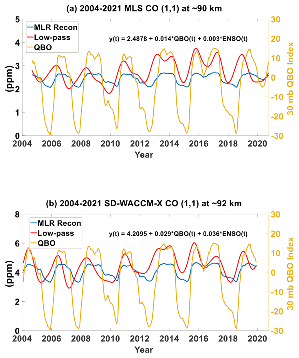
Figure 10(a) MLS CO (1,1) at ∼90 km reconstructed using multiple linear projection (MLR), low pass filtered and the 30 mb QBO index from 2004 until 2020. (b) Same as (a) but for SD-WACCM-X CO (1,1) at ∼92 km. Equations within the subplots are the MLR fits.
6.4 Quantifying the QBO response using multiple linear projection analysis and a low-pass filter
The previous subsection found that QBO and ENSO variabilities are present in both MLS CO hμ′ and SD-WACCM-X CO hμ′. In this section, we quantify the changes in MLS CO hμ′ or SD-WACCM-X CO hμ′ due to QBO. We do not quantify the changes due to ENSO because there were only a few events during our data span. Hence, any estimated response may be biased. We use multiple linear projection (MLR) to estimate the response of MLS CO hμ′ or SD-WACCM-X CO hμ′ to the QBO. Finally, we use the same MLR to reconstruct the time-series with the QBO index and then compare this reconstruction with a low-pass filtered version of the time-series. Note that while an MLR analysis offers an estimate of the response of one parameter to another, the reconstructed time-series using these MLR coefficients constrains the fluctuations to either be in-phase or completely anti-phase of the other parameter. It also assumes that the amplitude fluctuations are the same as that of the other time-series. For example, in the case of MLS CO hμ′ and the QBO index, the MLR reconstruction of MLS CO hμ′ can only be a time-series that is either completely in-phase with the QBO index or completely anti-phase. The overall fluctuation of the reconstruction will also only be a multiple of the QBO index time-series. With the low-pass filtered time-series, we can reconstruct the time-series that accounts for non-in-phase or non-anti-degree phase differences. The low-pass filtered time-series also accounts for the exact amplitude fluctuations as a function of time. Thus, in the case of MLS CO hμ′ and the QBO index, the low-pass filtered MLS CO hμ′ will reveal how dominant QBO periodicities are.
Figure 10 shows our MLR analysis and our low-pass filtering of MLS CO hμ′ and SD-WACCM-X CO hμ′ to quantify the responses of these parameters to QBO and ENSO. Figure 9 showed that the phase-relation between MLS CO hμ′ or SD-WACCM-X CO hμ′ and the QBO index were consistent for all years. However, the phase-relation between MLS CO hμ′ or SD-WACCM-X CO hμ′ and the QBO index changed. In this figure, we separate this analysis. Figure 10a and b focuses on the QBO response, while Fig. 10c to f focuses on the ENSO response.
Figure 10a shows the de-seasonalized MLS CO hμ′ from 2004 until 2020, reconstructed using an MLR (hereafter MLR recon MLS CO hμ′) and filtered with a fifth order low-pass filter with a cut-off period of 6 months (hereafter low-pass filtered MLS CO hμ′). The equation within the plot shows the MLR coefficients between the de-seasonalized MLS CO hμ′ and the QBO and ENSO indices. However, for this plot, we will ignore the coefficients for ENSO because, as mentioned above and as will be shown later, the phase relationship changes. Both reconstructions are overplotted with the QBO index. Figure 10b shows the same as Fig. 10a but for SD-WACCM-X CO hμ′. Figure 10a shows a QBO MLR coefficient of 0.014 for MLS CO hμ′. The MLR fit has p value = 0.002, which is less than 0.05 indicating statistical significance. With this value, MLS CO hμ′ increases by around 0.21 ppm or a +8 % variation ( % variation where 2.49 is the temporal mean included in the MLR equation) when the QBO index is at the typical peak westerly value of around +15 m s−1. On the other hand, MLS CO hμ′ decreases by around −0.42 ppm or a −16 % variation when the QBO index is at the typical peak easterly value of around −30 m s−1. Figure 10a also shows that the low-pass filtered MLS CO hμ′ is dominated by low-frequency periodicities, whose combination yields a time-series that is dominated by QBO-like fluctuations. The time-series looks very similar to MLR recon MLS CO hμ′ and the QBO index. Using the standard deviation of the low-pass filtered MLS CO hμ′ as a measure of the variation, we calculate a variation of ∼0.9 ppm which is slightly higher than the 0.63 ppm variation estimated with the MLR coefficients. Comparing the low pass filtered MLS CO hμ′ and the QBO index further shows that peak westerly phase values in the QBO index occur just after the local maximum values. This is consistent with the cross-wavelet spectrum arrows in Fig. 9c. Figure 10b shows a QBO MLR coefficient of 0.029 for SD-WACCM-X CO hμ′. The MLR fit has p value less than 0.0001, indicating statistical significance (p value <0.05). With this value, SD-WACCM-X CO hμ′ increases by around 0.44 ppm or a +10 % variation when the QBO index is at the typical peak westerly value. SD-WACCM-X CO hμ′ decreases by around 0.88 ppm or a −20 % variation when the QBO index is at the typical peak easterly value.
Figure 10b also shows that the low-pass filtered SD-WACCM-X CO hμ′ is also dominated by QBO-like fluctuations that are like the MLR recon SD-WACCM-X CO hμ′ but slightly larger in variance at around 1.52 ppm and corrected for the phase differences determined by the cross-wavelet spectrum arrows in Fig. 9d.
This work uses 17 years of CO observations provided by the microwave limb sounder (MLS) on-board the Aura satellite to analyze the seasonal and interannual variability of the DW1 component of upper mesospheric CO. These were then compared to simulations by the specified dynamics – whole atmosphere community climate model with ionosphere/thermosphere extension (SD-WACCM-X). Our results showed that the largest MLS CO μ′ and SD-WACCM-X CO μ′ are above 80 km. For MLS CO μ′, its latitude structure in March equinox above 80 km resembles that of the (1,1) mode although there is an interhemispheric asymmetry with the location of their mid-latitude peaks. On the other hand, the latitude structure of MLS CO μ′ in June solstice above 80 km resembles that of the distorted (1,1) mode. For SD-WACCM-X CO μ′, its latitude structure in March equinox above 80 km also resembles that of the (1,1) mode, but there is negligible interhemispheric asymmetry with the location of their mid-latitude peaks. Also, SD-WACCM-X simulates two pulses of this (1,1) mode feature between 80 km and 95 km while MLS observes only one pulse. SD-WACCM-X CO μ′ in June solstice also resembles that of the distorted (1,1) mode, but SD-WACCM-X simulates two pulses of this mode.
To explain MLS CO μ′ and SD-WACCM-X CO μ′, we first looked at MLS T′, SABER T′ and SD-WACCM-X T′. All three show the (1,1) mode in March equinox and the distorted (1,1) mode in June solstice. However, the (1,1) mode in March equinox for MLS T′ shows more interhemispheric asymmetry in terms of the locations of the mid-latitude peaks. Also, SD-WACCM-X T′ showed two pulses of the (1,1) mode and distorted (1,1) mode. These gave hints that the mechanisms driving CO μ′ may indeed be related to the mechanisms behind T′.
To determine what drives CO μ′ and how it relates to T′, we first did a tendency analysis involving the continuity equation. Our tendency analysis revealed that, in SD-WACCM-X, vertical advection in both March equinox and June solstice has the closest magnitude and latitude–altitude structure to the time-derivative term. We then determined if the same mechanism holds for the observations by using the adiabatic displacement method. Our adiabatic displacement method determined that for March equinox CO μ′ and CO μw′ in observations and simulations were very similar. However, for June solstice, MLS CO μ′ and CO μw′ are only similar between latitudes 30∘ S and 60∘ N. The simulations were very similar for all latitudes
After comparing CO μ′ and CO μw′ in observations and simulations, we probed deeper into CO's (1,1) mode. Our results showed that for seasonal and interannual timescales the observed and simulated CO hμ′ and CO hw′ are highly correlated, with correlation coefficients of at least 0.97.
Finally, we characterized the interannual variability present in CO μ′. A cross-wavelet MLR analysis and low-pass filtering indicate that MLS CO hμ′ is enhanced by around 8 % during the westerly phase of the QBO and is reduced by around 16% during the easterly phase of the QBO. SD-WACCM-X CO hμ′ is also enhanced by around 10 % during the westerly phase of the QBO and is also reduced by around 20 % during the easterly phase of the QBO.
A cross-wavelet between MLS CO hμ′ at ∼90 km and the ENSO index shows that MLS CO hμ′ and the ENSO index both have statistically significant oscillations, with periods of around ∼30 months between years 2008 and 2012. This coincides with the strong 2010–2011 La Niña event. On the other hand, a cross-wavelet between SD-WACCM-X CO hμ′ at ∼92 km and the ENSO index shows that SD-WACCM-X CO hμ′ and ENSO index both have statistically significant oscillations with periods between 24 to 36 months from 2006 until 2016. This coincides with both the strong 2010–2011 La Niña event and the strong 2015–2016 El Niño event. However, the lack of ENSO events indicate that these may just be coincidental.
From these results, we can conclude that the global structure of upper mesospheric MLS CO's DW1 component is primarily driven by DW1-induced vertical advection over all latitudes during equinox seasons and over all latitudes except the winter middle to high latitudes during solstice seasons. On the other hand, the global structure of upper mesospheric SD-WACCM-X CO's DW1 component is primarily driven by DW1-induced vertical advection over all latitudes for both equinox and solstice seasons. We also conclude that the dominant DW1 tidal mode in upper mesospheric MLS CO DW1 and SD-WACCM-X CO DW1 is the (1,1) mode. In addition, we find that the interannual variability of MLS CO (1,1) and SD-WACCM-X CO (1,1) is primarily driven by the QBO and ENSO's effects on DW1-induced vertical advection. These conclusions suggest that we can use CO as a tracer for vertical advection due to the DW1 tide and the (1,1) mode on seasonal and interannual timescales.
Figure A1 shows the CO averaged for all September equinox and for all December solstice as observed by MLS and as simulated by SD-WACCM-X. Figure A2 shows CO μ′ in September equinox and in December solstice as observed by MLS and as simulated by SD-WACCM-X. Figure A3 shows T′ in September equinox and in December solstice as observed by MLS and SABER and as simulated by SD-WACCM-X. The similarities and differences of these parameters between September equinox and December solstice are the same as those in the comparison of these parameters between March equinox and June solstice.

Figure A1Daily mean zonal-mean component of (a) MLS CO in September equinox, (b) SD-WACCM-X CO in September equinox, (c) MLS CO in December solstice and (d) SD-WACCM-X CO in December solstice. All are in units of ppm.
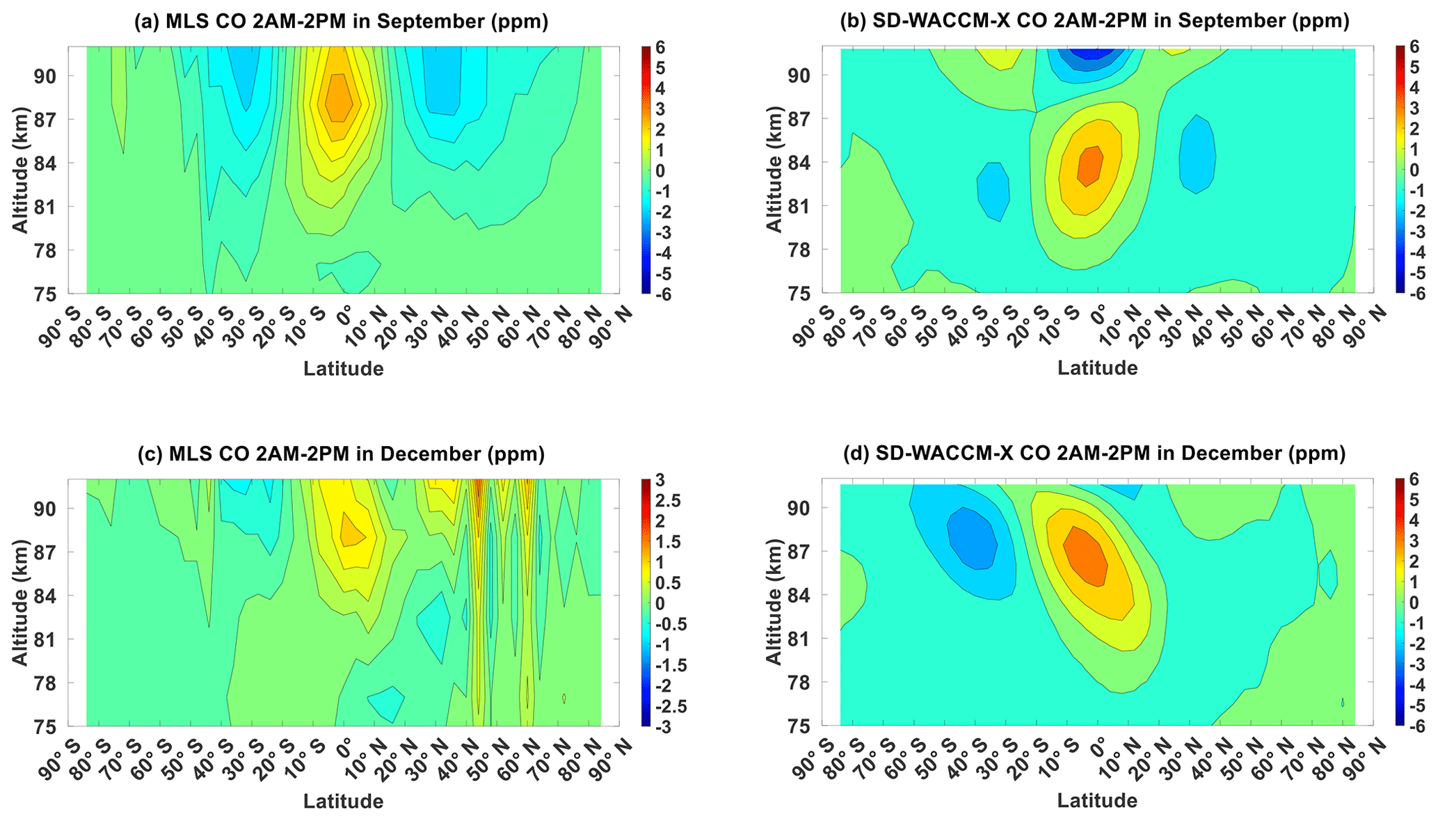
Figure A2Migrating diurnal tide component of (a) MLS CO in September equinox, (b) SD-WACCM-X CO in September equinox, (c) MLS CO in December solstice and (d) SD-WACCM-X CO in December solstice. All are in units of ppm.
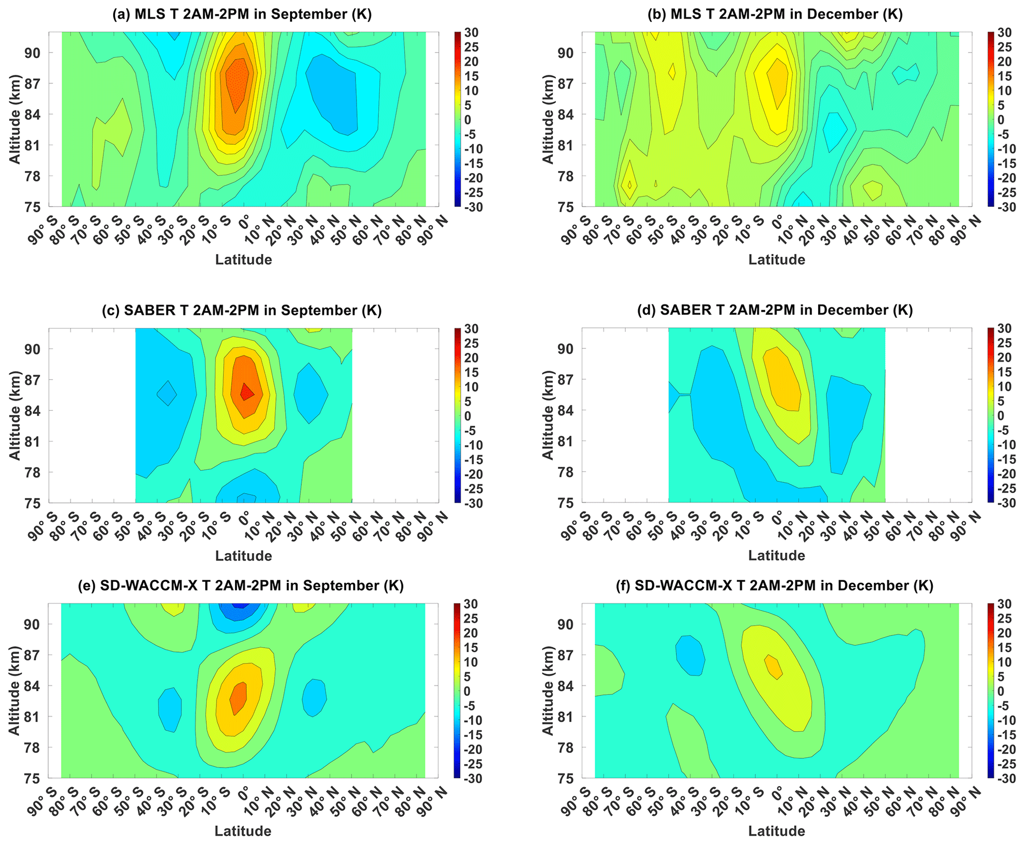
Figure A3Migrating diurnal tide component of (a) MLS temperature in September equinox, (b) MLS temperature in December solstice, (c) SABER temperature in September equinox, (d) SABER temperature in December solstice, (e) SD-WACCM-X temperature in September equinox and (f) SD-WACCM-X temperature in December solstice. All are in units of K.
Figure B1 shows the chemical production term, chemical loss term, zonal advection term, meridional advection term, eddy diffusion term and molecular diffusion term of CO for March equinox. Figure B1a shows the chemical production term peaking to around 2 ppm d−1 over the Equator above 90 km. Figure B1b shows the chemical loss term peaking to around 2 ppm d−1 over the northern high latitudes below 80 km. Figure B1c shows the zonal advection term peaking to around 1 ppm d−1 over the Equator above 85 km. Figure B1d shows the meridional advection term peaking to around 4 ppm d−1 over the mid-latitudes above 90 km. Figure B1e shows the eddy diffusion term peaking to around 0.6 ppm d−1 over the low-latitudes above 90 km. Figure B1f shows the molecular diffusion term peaking to around 0.2 ppm d−1s also over the low-latitudes above 90 km. These values are all clearly significantly lower than the vertical advection term in Fig. 4b.
Figure B2 shows the chemical production term, chemical loss term, zonal advection term, meridional advection term, eddy diffusion term and molecular diffusion term of CO for June solstice. Figure B2a shows the chemical production term peaking to around 4 ppm d−1 also over northern high latitudes above 90 km. Figure B2b shows the chemical loss term peaking to around 3 ppm d−1 also over southern high latitudes below 80 km. Figure B2c shows the zonal advection term peaking to around 0.6 ppm d−1 over the northern mid-latitudes above 85 km. Figure B2d shows the meridional advection term peaking to around 4 ppm d−1 over the mid-latitudes above 80 km. Figure B2e shows the eddy diffusion term peaking to around 0.3 ppm d−1 over the northern low-latitudes above 90 km. Figure B2f shows the molecular diffusion term peaking to around 0.1 ppm d−1s also over the northern low-latitudes above 90 km. Unlike March equinox, there are regions where the chemical production term and meridional advection term are comparable to the vertical advection term. For the chemical production term, its values are not too far from the vertical advection term over the northern high-latitudes above 90 km. For the meridional advection term, its values are not too far from the vertical advection term over the northern mid-latitudes between 80 and 90 km. These terms could function as secondary mechanisms over these regions.
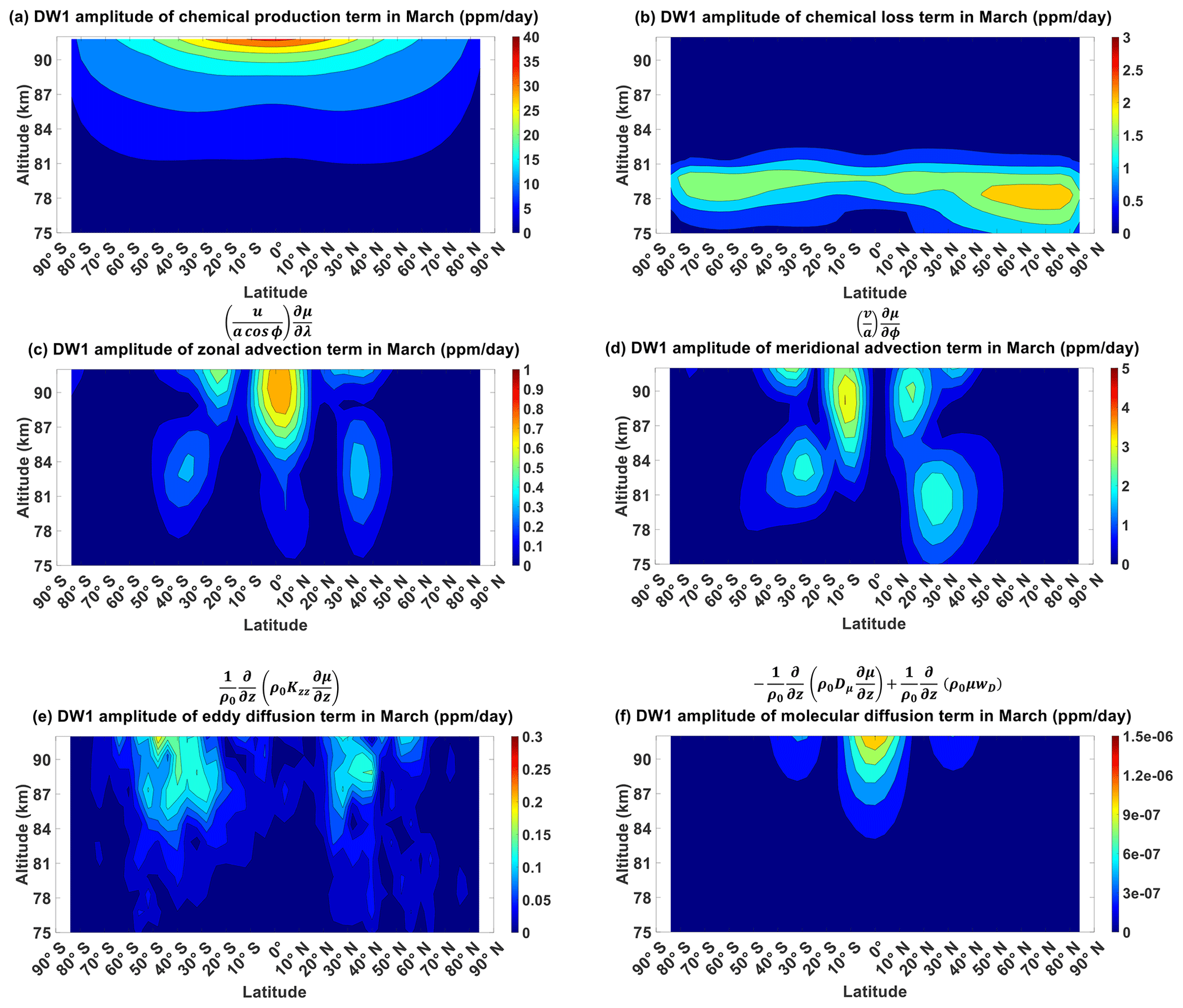
Figure B1Migrating diurnal tide component in March equinox of (a) CO's chemical production term, (b) CO's chemical loss term, (c) CO's zonal advection term, (d) CO's meridional advection term, (e) CO's eddy diffusion term and (f) CO's molecular diffusion term. All are in units of ppm d−1.
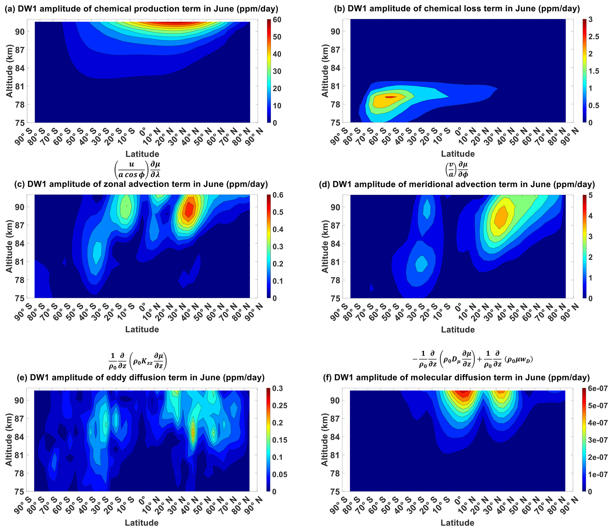
Figure B2Migrating diurnal tide component in June solstice of (a) CO's chemical production term, (b) CO's chemical loss term, (c) CO's zonal advection term, (d) CO's meridional advection term, (e) CO's eddy diffusion term and (f) CO's molecular diffusion term. All are in units of ppm d−1.
Figure C1 identifies interannual phenomena found in hT′, and here we show that the features are very similar to that for hμ′ in Fig. 9. Figure C1a shows the time-series of MLS hT′ at ∼90 km, SD-WACCM-X hT′ at ∼92 km and the QBO index. Figure C1b shows the time-series of MLS hT′ at ∼90 km, SD-WACCM-X hT′ at ∼92 km and the MEI index. Figure C1c shows the cross-wavelet spectrum between MLS hT′ and the QBO index. Figure C1c reveals that both MLS hT′ and the QBO index have a statistically significant oscillation with periods of around 24 months. It is statistically significant between 2005 and 2018. The arrows are pointed slightly upward, which indicate that MLS hT′ peak slightly ahead of the QBO index. The arrows also indicate that MLS hT′ increases during the westerly phase of the QBO while it decreases during the easterly phase of the QBO.
Figure C1d shows the cross-wavelet spectrum between MLS hT′ and the MEI index. This spectrum reveals that both MLS hT′ and the MEI index have a statistically significant oscillation of around 30 months between 2008 and 2012. This does coincide with a strong La Niña event. The arrows are pointed almost fully to the left, which indicate that MLS hT′ and ENSO are anti-correlated. MLS hT′ increases during La Niña, and it decreases during El Niño.
Figure C1e shows the cross-wavelet spectrum between SD-WACCM-X hT′ and the QBO index. This spectrum reveals that both SD-WACCM-X hT′ and the QBO index have a statistically significant oscillation with periods ranging from 20 to 30 months, and the statistical significance is found throughout all years. From 2015 to 2020, both have a statistically significant oscillation with a period of around 15 to 20 months. Like MLS hT′, the arrows are pointed slightly upward, which indicate that SD-WACCM-X hT′ peak slightly ahead of the QBO index and that SD-WACCM-X hT′ increases during the westerly phase of the QBO, while it decreases during the easterly phase of the QBO.
Figure C1f shows the cross-wavelet spectrum between SD-WACCM-X hT′ and the MEI index. This spectrum reveals that both have a statistically significant oscillation with period of around 24 to 36 months. This period of statistical significance lasts from 2006 to 2016. Like MLS hT′, the arrows are pointed almost fully to the left, which indicate that SD-WACCM-X hT′ and ENSO are almost anti-correlated and that SD-WACCM-X hT′ increases during La Niña and it decreases during El Niño.
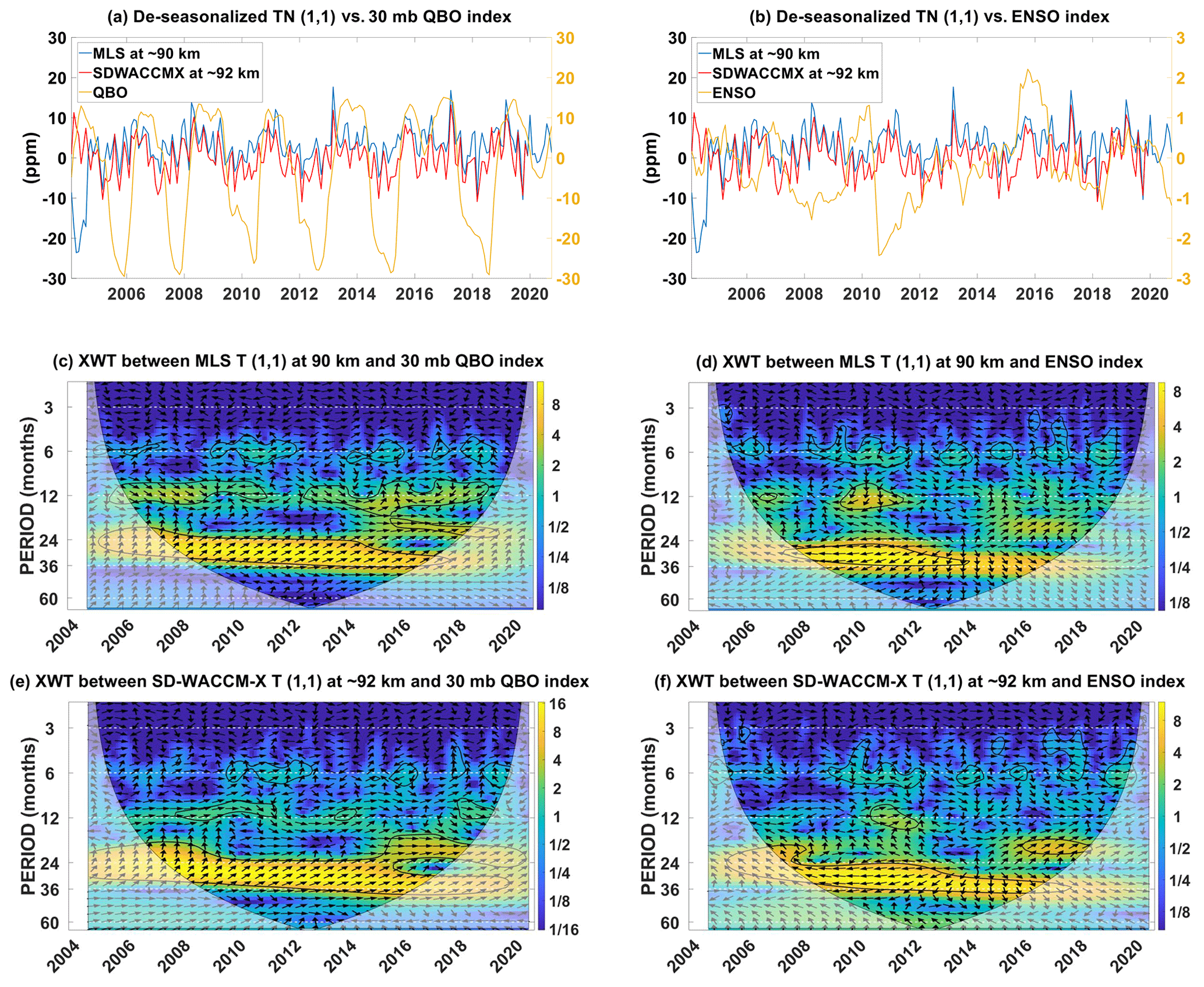
Figure C1(a) De-seasonalized time-series of MLS temperature (1,1) at ∼90 km, SD-WACCM-X temperature (1,1) at ∼92 km and the QBO index. (b) De-seasonalized time-series of MLS temperature (1,1) at ∼90 km, SD-WACCM-X temperature (1,1) at ∼92 km and the ENSO index. (c) Cross-wavelet spectrum between MLS temperature (1,1) at ∼90 km and the QBO index. (d) Cross-wavelet spectrum between MLS temperature (1,1) at ∼90 km and the ENSO index. (e) Cross-wavelet spectrum between SD-WACCM-X temperature (1,1) at ∼92 km and the QBO index. (f) Cross-wavelet spectrum between SD-WACCM-X temperature (1,1) at ∼92 km and the ENSO index.
As a component of the community earth system model, WACCM-X source code are publicly available at http://www.cesm.ucar.edu (NCAR, 2023).
The SABER dataset presented in this paper is accessible from the SABER website: http://saber.gats-inc.com/data.php (SABER GATS, 2022). The MLS dataset presented in this paper is accessible from the MLS website: https://aura.gsfc.nasa.gov/mls.html (NASA Jet Propulsion Laboratory, 2022). QBO index is accessible from http://www.cpc.ncep.noaa.gov/data/indices/qbo.u30.index (National Weather Service Climate Prediction Center, 2022). ENSO/MEI index is accessible from https://psl.noaa.gov/enso/mei/ (Physical Sciences Laboratory, 2022).
Conceptualization and investigation were done by CCJHS, DLW and JNL. Formal analysis and visualization were done by CCJHS with help and supervision from DLW and JNL. Data curation on MLS data was done by JNL. Data curation on SABER data was done by CCJHS. Access to SD-WACCM-X was provided by LQ and HL. SD-WACCM-X was run on Cheyenne (https://doi.org/10.5065/D6RX99HX) provided by NCAR's Computational and Information Systems Laboratory, sponsored by the National Science 510 Foundation. DLW, JNL and LCC provided funding acquisition. CCJHS wrote the original draft of the paper with help from DLW and JNL. All authors reviewed and edited the paper.
The contact author has declared that none of the authors has any competing interests.
Publisher’s note: Copernicus Publications remains neutral with regard to jurisdictional claims in published maps and institutional affiliations.
Cornelius Csar Jude H. Salinas and Loren C. Chang acknowledge the Taiwan National Science and Technology Council as well as the Higher Education SPROUT Project grant to the Center for Astronautical Physics and Engineering from the Taiwan Ministry of Education. The work of Dong L. Wu and Jae N. Lee was supported by NASA’s TSIS project and Sun-Climate research. Liying Qian and Hanli Liu acknowledges support from NASA. The National Center for Atmospheric Research is a major facility sponsored by the National Science Foundation under cooperative agreement no. 1852977.
This research has been supported by the Taiwan National Science and Technology Council grants 111-2636-M-008-004, 107-2923-M-008-001-MY3 and 110-2923-M-008-005-MY3. This research has also been supported by NASA grants 80NSSC19K0278, 80NSSC20K0189, NNH19ZDA001N-HGIO, NNH19ZDA001N-HSR and 80NSSC20K1323.
This paper was edited by John Plane and reviewed by two anonymous referees.
Akmaev, R. A. and Shved, G. M.: Modelling of the composition of the lower thermosphere taking account of the dynamics with applications to tidal variations of the [OI] 5577 Å airglow, J. Atmos. Terr. Phys., 42, 705–716, 1980.
Allen, D. R., Stanford, J. L., López-Valverde, M. A., Nakamura, N., Lary, D. J., Douglass, A. R., Cerniglia, M. C., Remedios, J. J., and Taylor, F. W.: Observations of middle atmosphere CO from the UARS ISAMS during the early northern winter 1991/92, J. Atmos. Sci., 56, 563–583, 1999.
Allen, D. R., Stanford, J. L., Nakamura, N., Lopez-Valverde, M. A., Lopez-Puertas, M., Taylor, F. W., and Remedios, J.J.: Antarctic polar descent and planetary wave activity observed in ISAMS CO from April to July 1992, Geophys. Res. Lett., 27, 665–668, 2000.
Angelats i Coll, M. and Forbes, J. M.: Dynamical influences on atomic oxygen and 5577 Å emission rates in the lower thermosphere, Geophys. Res. Lett., 25, 461–464, 1998.
Brasseur, G. P. and Solomon, S.: Aeronomy of the middle atmosphere: Chemistry and physics of the stratosphere and mesosphere, vol. 32, Springer Science & Business Media, https://doi.org/10.1007/1-4020-3824-0_3, 2006.
Burrage, M. D., Hagan, M. E., Skinner, W. R., Wu, D. L., and Hays, P. B.: Long-term variability in the solar diurnal tide observed by HRDI and simulated by the GSWM, Geophys. Res. Lett., 22, 2641–2644, https://doi.org/10.1029/95GL02635, 1995.
Cen, Y., Yang, C., Li, T., Russell III, J. M., and Dou, X.: Suppressed migrating diurnal tides in the mesosphere and lower thermosphere region during El Niño in northern winter and its possible mechanism, Atmos. Chem. Phys., 22, 7861–7874, https://doi.org/10.5194/acp-22-7861-2022, 2022.
Chapman, S. and Lindzen, R. S.: Atmospheric tides, 200 pp., Reidel, D., Norwell, Mass., ISBN 9789401034012, 1970.
Dawkins, E. C. M., Feofilov, A., Rezac, L., Kutepov, A. A., Janches, D., Höffner, J., Chu, X., Lu, X., Mlynczak, M. G., and Russell III, J.: Validation of SABER v2. 0 operational temperature data with ground-based lidars in the mesosphere-lower thermosphere region (75–105 km), J. Geophys. Res.-Atmos., 123, 9916–9934, 2018.
Forbes, J. M.: Tidal and planetary waves. The Upper Mesosphere and Lower Thermosphere: A Review of Experiment and Theory, Geophys. Monogr. Ser, 87, 67–87, 1995.
Forbes, J. M. and Wu, D.: Solar tides as revealed by measurements of mesosphere temperature by the MLS experiment on UARS, J. Atmos. Sci., 63, 1776–1797, 2006.
Gan, Q., Du, J., Ward, W. E., Beagley, S. R., Fomichev, V. I., and Zhang, S.: Climatology of the diurnal tides from eCMAM30 (1979 to 2010) and its comparison with SABER, Earth Planets Space, 66, 1–24, 2014.
Garcia, R. R., López-Puertas, M., Funke, B., Marsh, D. R., Kinnison, D. E., Smith, A. K., and González-Galindo, F.: On the distribution of CO2 and CO in the mesosphere and lower thermosphere, J. Geophys. Res.-Atmos., 119, 5700–5718, 2014.
Garcia, R. R., Smith, A. K., Kinnison, D. E., Cámara, Á. D. L., and Murphy, D. J.: Modification of the gravity wave parameterization in the Whole Atmosphere Community Climate Model: Motivation and results, J. Atmos. Sci., 74, 275–291, 2017.
García-Comas, M., López-Puertas, M., Marshall, B. T., Wintersteiner, P. P., Funke, B., Bermejo-Pantaleón, D., Mertens, C. J., Remsberg, E. E., Gordley, L. L., Mlynczak, M. G., and Russell III, J. M.: Errors in Sounding of the Atmosphere using Broadband Emission Radiometry (SABER) kinetic temperature caused by non-local-thermodynamic-equilibrium model parameters, J. Geophys. Res.-Atmos., 113, https://doi.org/10.1029/2008JD010105, 2008.
Grinsted, A., Moore, J. C., and Jevrejeva, S.: Application of the cross wavelet transform and wavelet coherence to geophysical time series, Nonlin. Processes Geophys., 11, 561–566, https://doi.org/10.5194/npg-11-561-2004, 2004.
Groves, G. V.: Hough components of ozone heating, J. Atmos. Terr. Phys., 44, 111–121, 1982a.
Groves, G. V.: The vertical structure of atmospheric oscillations formulated by classical tidal theory, Plant. Space Sci., 30, 219–244, 1982b.
Gurubaran, S., Rajaram, R., Nakamura, T., and Tsuda, T.: Interannual variability of diurnal tide in the tropical mesopause region: a signature of the El Niño-Southern Oscillation (ENSO), Geophys. Res. Lett., 32, L13805, https://doi.org/10.1029/2005gl022928, 2005.
Gurubaran, S., Rajaram, R., Nakamura, T., Tsuda, T., Riggin, D., and Vincent, R. A.: Radar observations of the diurnal tide in the tropical mesosphere-lower thermosphere region: Longitudinal variabilities, Earth Planets Space, 61, 513–524, 2009.
Hagan, M. E. and Forbes, J. M.: Migrating and nonmigrating diurnal tides in the middle and upper atmosphere excited by tropospheric latent heat release, J. Geophys. Res.-Atmos., 107, ACL 6-1–ACL 6-15, https://doi.org/10.1029/2001JD001236, 2002.
Jones Jr., M., Forbes, J. M., and Hagan, M. E. Tidal-induced net transport effects on the oxygen distribution in the thermosphere, Geophys. Res. Lett., 41, 5272–5279, 2014.
Kogure, M. and Liu, H.: DW1 tidal enhancements in the equatorial MLT during 2015 El Niño: The relative role of tidal heating and propagation, J. Geophys. Res.-Space, 126, e2021JA029342, https://doi.org/10.1029/2021JA029342, 2021.
Kunz, A., Pan, L. L., Konopka, P., Kinnison, D. E., and Tilmes, S.: Chemical and dynamical discontinuity at the extratropical tropopause based on START08 and WACCM analyses, J. Geophys. Res.-Atmos., 116, https://doi.org/10.1029/2011JD016686, 2011.
Kutepov, A. A., Feofilov, A. G., Marshall, B. T., Gordley, L. L., Pesnell, W. D., Goldberg, R. A., and Russell III, J. M.: SABER temperature observations in the summer polar mesosphere and lower thermosphere: Importance of accounting for the CO2 ν2 quanta V–V exchange, Geophys. Res. Lett., 33, https://doi.org/10.1029/2006GL026591, 2006.
Lee, J. N., Wu, D. L., Manney, G. L., Schwartz, M. J., Lambert, A., Livesey, N. J., Minschwaner, K. R., Pumphrey, H. C., and Read, W. G.: Aura Microwave Limb Sounder observations of the polar middle atmosphere: Dynamics and transport of CO and H2O, J. Geophys. Res.-Atmos., 116, https://doi.org/10.1029/2010JD014608, 2011.
Lieberman, R. S.: Long-term variations of zonal mean winds and (1, 1) driving in the equatorial lower thermosphere, J. Atmos. Sol.-Terr. Phy., 59, 1483–1490, 1997.
Lieberman, R. S., Riggin, D. M., Ortland, D. A., Nesbitt, S. W., and Vincent, R. A.: Variability of mesospheric diurnal tides and tropospheric diurnal heating during 1997–1998, J. Geophys. Res.-Atmos., 112, https://doi.org/10.1029/2007jd008578, 2007.
Liu, H. L., Bardeen, C. G., Foster, B. T., Lauritzen, P., Liu, J., Lu, G., Marsh, D. R., Maute, A., McInerney, J. M., Pedatella, N. M., and Qian, L.: Development and validation of the Whole Atmosphere Community Climate Model with thermosphere and ionosphere extension (WACCM-X 2.0), J. Adv. Model. Earth Sy., 10, 381–402, 2018.
Liu, H., Sun, Y. Y., Miyoshi, Y., and Jin, H.: ENSO effects on MLT diurnal tides: A 21-year reanalysis data-driven GAIA model simulation, J. Geophys. Res.-Space Phys., 122, 5539–5549, https://doi.org/10.1002/2017JA024011, 2017.
Liu, J., Liu, H., Wang, W., Burns, A. G., Wu, Q., Gan, Q., Solomon, S. C., Marsh, D. R., Qian, L., Lu, G., and Pedatella, N. M.: First results from the ionospheric extension of WACCM-X during the deep solar minimum year of 2008, J. Geophys. Res.-Space, 123, 1534–1553, 2018.
Livesey, N. J., Read, W. G., Froidevaux, L., Lambert, A., Manney, G. L., Pumphrey, H. C., Santee, M. L., Schwartz, M. J., Wang, S., Cofield, R. E., Cuddy, D. T., Fuller, R. A., Jarnot, R. F., Jiang, J. H., Knosp, B. W., Stek, P. C., Wagner, P. A., and Wu, D. L.: Version 3.3 Level 2 data quality and description document, JPL D-33509, 3, 4–1, https://mls.jpl.nasa.gov/data/v3-3_data_quality_document.pdf (last access: January 2022), 2011.
Manney, G. L., Schwartz, M. J., Krüger, K., Santee, M. L., Pawson, S., Lee, J. N., Daffer, W. H., Fuller, R. A., and Livesey, N. J.: Aura Microwave Limb Sounder observations of dynamics and transport during the record-breaking 2009 Arctic stratospheric major warming, Geophys. Res. Lett., 36, https://doi.org/10.1029/2009GL038586, 2009.
Marsh, D. R.: Chemical–dynamical coupling in the mesosphere and lower thermosphere, in: Aeronomy of the Earth's Atmosphere and Ionosphere, 3–17, Springer, Dordrecht, https://doi.org/10.1007/978-94-007-0326-1_1, 2011.
Marsh, D. R. and Russell III, J. M.: A tidal explanation for the sunrise/sunset anomaly in HALOE low-latitude nitric oxide observations, Geophys. Res. Lett., 27, 3197–3200, 2000.
Marsh, D. R., Skinner, W. R., and Yudin, V. A.: Tidal influences on O2 atmospheric band dayglow: HRDI observations vs. model simulations, Geophys. Res. Lett., 26, 1369–1372, 1999.
Marsh, D. R., Mills, M. J., Kinnison, D. E., Lamarque, J. F., Calvo, N., and Polvani, L. M.: Climate change from 1850 to 2005 simulated in CESM1 (WACCM), J. Climate, 26, 7372–7391, 2013.
Mayr, H. G. and Mengel, J. G.: Interannual variations of the diurnal tide in the mesosphere generated by the quasi-biennial oscillation, J. Geophys. Res.-Atmos., 110, https://doi.org/10.1029/2004JD005055, 2005.
McLandress, C.: Seasonal variability of the diurnal tide: Results from the Canadian middle atmosphere general circulation model, J. Geophys. Res.-Atmos., 102, 29747–29764, 1997.
McLandress, C.: The seasonal variation of the propagating diurnal tide in the mesosphere and lower thermosphere. Part I: The role of gravity waves and planetary waves, J. Atmos. Sci., 59, 893–906, 2002a.
McLandress, C.: The seasonal variation of the propagating diurnal tide in the mesosphere and lower thermosphere. Part II: The role of tidal heating and zonal mean winds. J. Atmos. Sci., 59, 907–922, 2002b.
Mertens, C. J., Mlynczak, M. G., López-Puertas, M., Wintersteiner, P. P., Picard, R. H., Winick, J. R., Gordley, L. L., and Russell III, J. M.: Retrieval of mesospheric and lower thermospheric kinetic temperature from measurements of CO2 15 µm Earth Limb Emission under non-LTE conditions, Geophys. Res. Lett., 28, 1391–1394, 2001.
Mertens, C. J., Russell III, J. M., Mlynczak, M. G., She, C. Y., Schmidlin, F. J., Goldberg, R. A., López-Puertas, M., Wintersteiner, P. P., Picard, R. H., Winick, J. R., and Xu, X.: Kinetic temperature and carbon dioxide from broadband infrared limb emission measurements taken from the TIMED/SABER instrument, Adv. Space Res., 43, 15–27, 2009.
Minschwaner, K., Manney, G. L., Livesey, N. J., Pumphrey, H. C., Pickett, H. M., Froidevaux, L., Lambert, A., Schwartz, M. J., Bernath, P. F., Walker, K. A., and Boone, C. D.: The photochemistry of carbon monoxide in the stratosphere and mesosphere evaluated from observations by the Microwave Limb Sounder on the Aura satellite, J. Geophys. Res., 115, D13303, https://doi.org/10.1029/2009JD012654, 2010.
Mukhtarov, P., Pancheva, D., and Andonov, B.: Global structure and seasonal and interannual variability of the migrating diurnal tide seen in the SABER/TIMED temperatures between 20 and 120 km, J. Geophys. Res.-Space, 114, https://doi.org/10.1029/2008JA013759, 2009.
NCAR: WACCM-X source code are publicly available at http://www.cesm.ucar.edu (last access: January 2020), 2023.
NASA Jet Propulsion Laboratory: https://mls.jpl.nasa.gov/, last access: January 2022.
National Weather Service Climate Prediction Center: QBO index, http://www.cpc.ncep.noaa.gov/data/indices/qbo.u30.index, last access: January 2022.
Nguyen, V. and Palo, S. E.: Technique to produce daily estimates of the migrating diurnal tide using TIMED/SABER and EOS Aura/MLS, J. Atmos. Sol.-Terr. Phy., 105, 39–53, https://doi.org/10.1016/j.jastp.2013.07.008, 2013.
Oberheide, J. and Forbes, J. M.: Thermospheric nitric oxide variability induced by nonmigrating tides, Geophys. Res. Lett., 35, https://doi.org/10.1029/2008GL034825, 2008.
Oberheide, J., Hagan, M. E., and Roble, R. G.: Tidal signatures and aliasing in temperature data from slowly precessing satellites, J. Geophys. Res.-Space, 108, https://doi.org/10.1029/2002JA009585, 2003.
Pancheva, D., Mukhtarov, P., and Andonov, B.: Global structure, seasonal and interannual variability of the migrating semidiurnal tide seen in the SABER/TIMED temperatures (2002–2007), Ann. Geophys., 27, 687–703, https://doi.org/10.5194/angeo-27-687-2009, 2009.
Pedatella, N. M. and Liu, H. L.: Tidal variability in the mesosphere and lower thermosphere due to the El Niño-Southern Oscillation, Geophys. Res. Lett., 39, L19802, https://doi.org/10.1029/2012gl053383, 2012.
Pedatella, N. M. and Liu, H. L.: Influence of the El Niño Southern Oscillation on the middle and upper atmosphere, J. Geophys. Res.-Atmos., 118, 2744–2755, https://doi.org/10.1002/Jgra.50286, 2013.
Physical Science Laboratory: ENSO/MEI index, https://psl.noaa.gov/enso/mei/, last access: January 2022.
Pramitha, M., Kumar, K. K., Ratnam, M. V., Praveen, M., and Bhaskara Rao, S. V.: Stratospheric Quasi Biennial Oscillation Modulations of Migrating Diurnal Tide in the Mesosphere and Lower Thermosphere Over the Low and Equatorial Latitudes, J. Geophys. Res.-Space, 126, e2020JA028970, https://doi.org//10.1029/2020JA028970, 2021.
Remsberg, E. E., Marshall, B. T., Garcia-Comas, M., Krueger, D., Lingenfelser, G. S., Martin-Torres, J., Mlynczak, M. G., Russell III, J. M., Smith, A. K., Zhao, Y., and Brown, C.: Assessment of the quality of the Version 1.07 temperature-versus-pressure profiles of the middle atmosphere from TIMED/SABER, J. Geophys. Res.-Atmos., 113, https://doi.org/10.1029/2008JD010013, 2008.
Richter, J. H., Sassi, F., and Garcia, R. R.: Toward a physically based gravity wave source parameterization in a general circulation model, J. Atmos. Sci., 67, 136–156, 2010.
Rienecker, M. M., Suarez, M. J., Gelaro, R., Todling, R., Bacmeister, J., Liu, E., Bosilovich, M. G., Schubert, S. D., Takacs, L., Kim, G. K., and Bloom, S.: MERRA: NASA's modern-era retrospective analysis for research and applications, J. Climate, 24, 3624–3648, 2011.
Russell III, J. M., Mlynczak, M. G., Gordley, L. L., Tansock Jr., J. J., and Esplin, R. W.: October. Overview of the SABER experiment and preliminary calibration results, in: Optical spectroscopic techniques and instrumentation for atmospheric and space research III, Vol. 3756, 277–288, SPIE, https://doi.org/10.1117/12.366382, 1999.
SABER GATS: https://saber.gats-inc.com/data.php, last access: January 2022.
Salinas, C. C. J. H., Chang, L. C., Liang, M. C., Yue, J., Qian, L., Gan, Q., Chiu, Y. C., Russell III, J., and Mlynczak, M.: Local-time variabilities of March equinox daytime SABER CO2 in the upper mesosphere and lower thermosphere region, J. Geophys. Res.-Space, 125, p.e2019JA027039, https://doi.org/10.1029/2019JA027039, 2020.
Salinas, C. C. J. H., Chang, L. C., Yue, J., Qian, L., Gan, Q., Russell III, J., and Mlynczak, M.: Estimating the Migrating Diurnal Tide Component of Mesospheric Water Vapor, J. Geophys. Res.-Space, e2021JA030187, https://doi.org/10.1029/2021JA030187, 2022.
Shepherd, G. G., McLandress, C., and Solheim, B. H.: Tidal influence on O (1S) Airglow emission rate distributions at the geographic equator as observed by WINDII, Geophys. Res. Lett., 22, 275–278, 1995.
Shepherd, G. G., Roble, R. G., McLandress, C., and Ward, W. E.: WINDII observations of the 558 nm emission in the lower thermosphere: the influence of dynamics on composition, J. Atmos. Sol.-Terr. Phy., 59, 655–667, 1997.
Smith, A. K., Marsh, D. R., Mlynczak, M. G., and Mast, J. C.: Temporal variations of atomic oxygen in the upper mesosphere from SABER, J. Geophys. Res.-Atmos., 115, https://doi.org/10.1029/2009JD013434, 2010.
Smith, A. K., Garcia, R. R., Marsh, D. R., and Richter, J. H.: WACCM simulations of the mean circulation and trace species transport in the winter mesosphere, J. Geophys. Res.-Atmos., 116, https://doi.org/10.1029/2011JD016083, 2011.
Vincent, R. A., Kovalam, S., Fritts, D. C., and Isler, J. R.: Long-term MF radar observations of solar tides in the low-latitude mesosphere: Interannual variability and comparisons with the GSWM, J. Geophys. Res.-Atmos., 103, 8667–8683, 1998.
Ward, W. E.: A simple model of diurnal variations in the mesospheric oxygen nightglow, Geophys. Res. Lett., 26, 3565–3568, 1999.
Waters, J. W., Froidevaux, L., Harwood, R. S., Jarnot, R. F., Pickett, H. M., Read, W. G., Siegel, P. H., Cofield, R. E., Filipiak, M. J., Flower, D. A., and Holden, J. R.: The earth observing system microwave limb sounder (EOS MLS) on the Aura satellite, IEEE T. Geosci. Remote, 44, 1075–1092, 2006.
Wu, D. L., Hays, P. B., and Skinner, W. R.: A least squares method for spectral analysis of space-time series, J. Atmos. Sci., 52, 3501–3511, 1995.
Wu, Q., Ortland, D. A., Killeen, T. L., Roble, R. G., Hagan, M. E., Liu, H. L., Solomon, S. C., Xu, J., Skinner, W. R., and Niciejewski, R. J.: Global distribution and interannual variations of mesospheric and lower thermospheric neutral wind diurnal tide: 1. Migrating tide, J. Geophys. Res.-Space, 113, https://doi.org/10.1029/2007JA012542, 2008.
Xu, J., Smith, A. K., Liu, H. L., Yuan, W., Wu, Q., Jiang, G., Mlynczak, M. G., Russell Iii, J. M., and Franke, S. J.: Seasonal and quasi-biennial variations in the migrating diurnal tide observed by Thermosphere, Ionosphere, Mesosphere, Energetics and Dynamics (TIMED), J. Geophys. Res.-Atmos., 114, https://doi.org/10.1029/2008JD011298, 2009.
Zhang, S. P., Wiens, R. H., Solheim, B. H., and Shepherd, G. G.: Nightglow zenith emission rate variations in O (1 S) at low latitudes from wind imaging interferometer (WINDII) observations, J. Geophys. Res.-Atmos., 103, 6251–6259, 1998.
Zhang, X., Forbes, J. M., Hagan, M. E., Russell III, J. M., Palo, S. E., Mertens, C. J., and Mlynczak, M. G.: Monthly tidal temperatures 20–120 km from TIMED/SABER, J. Geophys. Res.-Space, 111, https://doi.org/10.1029/2005JA011504, 2006.
Zhou, X., Wan, W., Yu, Y., Ning, B., Hu, L., and Yue, X.: New approach to estimate tidal climatology from ground-and space-based observations, J. Geophys. Res.-Space Phys., 123, 5087–5101, https://doi.org/10.1029/2017JA024967, 2018.
- Abstract
- Introduction
- Satellite datasets and model
- Seasonality of the DW1 component of CO
- DW1 component of temperature
- Physical mechanisms of CO DW1
- (1,1) Hough mode component's seasonal and interannual variability
- Summary and conclusions
- Appendix A: Daily mean zonal-mean CO as well as the CO DW1 and temperature DW1 in September equinox and December solstice
- Appendix B: Tendency analysis terms
- Appendix C: Interannual phenomena in T′
- Code availability
- Data availability
- Author contributions
- Competing interests
- Disclaimer
- Acknowledgements
- Financial support
- Review statement
- References