Trends in measured and modeled lower stratospheric Antarctic vortex ozone over the past two decades

We analyze 2004 to 2023 winter/spring lower stratospheric Antarctic ozone data from the Aura Microwave Limb Sounder (MLS), along with similarly sampled profiles from two simulations from the Whole Atmosphere Community Climate Model (WACCM) run with specified dynamics. One of these simulations uses fixed surface organic halogens from 1998 onward. The interannual variability in MLS vortex-average ozone is well matched by WACCM, although WACCM shows a slightly smaller seasonal decrease. Probability density functions of vortex ozone profiles reveal slow increases in the smallest values; WACCM shows good agreement with MLS distribution shifts and simple linear trends. We also use multivariate linear regression with two periodic functions and a proxy for polar stratospheric clouds to derive trends in vortex-average ozone during September and October. Calculated trends are consistent with slow Antarctic vortex ozone recovery from the impact of ozone-depleting substances, with values between ∼ 5 and 16 ppbv yr⁻¹ in the 56–100 hPa layer. WACCM results agree well with those from MLS. The simulation with fixed surface organic halogens is consistent with zero trend. We also apply the Match technique, which follows MLS-observed parcels along trajectories to estimate vortex-average chemical ozone loss. Match estimates also show slow reductions in seasonal Antarctic ozone loss, although few of the Match results represent greater than two-sigma departures from zero. Our work confirms the emergence of ozone recovery, a key goal of the Aura mission, and underscores the importance of the 1987 Montreal Protocol and its Amendments in curtailing emissions of ozone-depleting substances.

1 Introduction

Early warnings were made in the 1970s (Molina and Rowland, 1974) regarding threats to the Earth's stratospheric ozone (O₃) layer from the decomposition of chlorofluorocarbons (CFCs) emitted at the surface by industrial activities. There were human health implications from increased ultraviolet (UV) radiation at the surface, which would arise from a reduction in UV absorption by stratospheric ozone. The subsequent discovery (Farman et al., 1985) of the recurring winter/spring ozone hole development over Antarctica has made polar ozone the subject of particularly intense studies. The 1987 Montreal Protocol and its subsequent Amendments curtailed the surface emissions of ozone-depleting substances (ODSs). The following decades saw a large increase in the database of polar (and global) ozone observations, as well as in the understanding of the main causes of this phenomenon and its evolution (e.g., Solomon, 1999; Chipperfield et al., 2022). In the polar regions, lower stratospheric ozone is destroyed during the cold winter and spring after the release of active chlorine from its stratospheric reservoir species (mainly HCl and ClONO₂), via heterogeneous chemical reactions enabled on the surfaces of polar stratospheric clouds (PSCs); chlorine and bromine species both contribute to the ozone destruction that peaks in September and October, after the return of sunlight to the polar regions.

As mentioned in recent Ozone Assessment Reports (WMO, 2018, 2022), a consensus has been building that, after a significant slowdown in global decreases of lower stratospheric and total column ozone abundances, we are now in the phase of ozone recovery from the effects of ODSs. The post-2000 period has been characterized by a decline in equivalent effective stratospheric chlorine (EESC), a metric used to represent the combined impact of total stratospheric chlorine and bromine abundances (Newman et al., 2007; Engel et al., 2018). EESC is related, in turn, to ODS emission changes at the surface; Lickley et al. (2024) have recently assessed how and why the estimates of EESC and global ozone recovery dates have evolved over the past two decades. There has been growing evidence for the emergence of lower stratospheric Antarctic ozone healing, although lower stratospheric ozone trends are hard to detect at other latitudes, including in the Arctic region, where larger dynamical variability occurs. Signs of the emergence of Antarctic ozone recovery since about the turn of the 21st century, following global decreases in ODSs, have been reported in analyses of a variety of data sets, including in situ data, satellite-based profiles and column ozone, coupled with model or data assimilation studies (e.g., Solomon et al., 2016; de Laat et al., 2017; Weber et al., 2018; Strahan and Douglass, 2018; Pazmiño et al., 2018; Chipperfield et al., 2022). Antarctic ozone profiles from ozonesondes and satellites showed that very small ozone abundances occurred seasonally after 1987, with destruction processes “saturating,” that is, insensitive to further increases in ODSs because there was no more ozone to destroy. Occurrences of near-zero ozone reached a maximum at the turn of the century, after which there were decreases in the saturation of ozone loss (Kuttippurath et al., 2018; Chipperfield et al., 2022). Quoting the latter reference, new results since 2018 support the findings that “the Antarctic ozone hole has generally diminished in size and depth since the year 2000.” More recent work by Pazmiño et al. (2023) employs a model-based passive ozone tracer and total ozone column observations since 1989 to analyze Antarctic ozone recovery based on three different metrics: maximum ozone loss at the end of winter, the onset dates for ozone loss, and a residual method that is coupled to regression analyses tied to the volume of PSCs (VPSC). Their study confirms the ozone recovery in the Antarctic, despite the increased interannual variability in the last decade compared to earlier periods. Also, according to Strahan et al. (2019), mid-September is when stratospheric ozone over Antarctica shows the largest sensitivity to decreasing ODSs and when Antarctic ozone recovery rates are strongest and most easily detected. The rate of decrease in Antarctic ozone is steepest in September; in October, there are more dynamically induced perturbations to the vortex, before its eventual breakup, typically in November or December.

For this work, we rely upon 20 years of ozone profiles retrieved from Aura Microwave Limb Sounder (MLS) measurements inside the Antarctic vortex, as detailed in Sect. 2. Measurements of global ozone as well as the variability in temperature and chemical processing inside the Arctic and Antarctic stratospheric vortices have been obtained nearly continuously by MLS since the Aura launch in July 2004 (e.g., Santee et al., 2005, 2011, 2024; Manney et al., 2011, 2023; Kuttippurath et al., 2015). By using this unique, continuous, well-sampled and stable ozone dataset, having the same regular data coverage over time, we avoid potential trend uncertainties that could arise from a merged record combining multiple datasets obtained using different measurement techniques with different spatio-temporal coverage within the analysis period. Two decades of high-quality MLS data provide a record of sufficient length for trend analysis. Moreover, we select abundance profiles obtained within the Antarctic vortex. This vortex-centered analysis takes into account variations in the dynamical characteristics (e.g., size, shape, and position) of the Antarctic vortex and thus better isolates the effects of chemical depletion in the ozone hole than the use of geographic latitude bins, which inevitably mix inside-vortex and midlatitude air. We compare the MLS data to results from two simulations from the Whole Atmosphere Chemistry Climate Model (WACCM), both using specified dynamics, but one of them having surface ODSs fixed at 1998 levels; after 4–5 years, the fixed-ODS conditions lead to nearly invariant EESC levels in the polar stratosphere. In Sect. 3, we analyze Antarctic ozone distributions from MLS and the WACCM simulations, with a focus on Probability Density Functions (PDFs) and simple linear trends; the use of these detailed PDFs for weekly data analyses from both MLS and similarly sampled model simulations is a novel approach for Antarctic ozone studies. In addition, we comment briefly on the observed and modeled HCl and HNO₃ distributions inside the Antarctic vortex. Trends in September and October vortex-average ozone profiles are then quantified using Multivariate Linear Regression (MLR), to obtain better fits to the time series and reduce the resulting trend uncertainties. To further motivate this work and distinguish it from past results, we also discuss another metric, namely trends in Antarctic ozone loss over the period from 2005 to 2023 computed using the Match technique, which follows a multitude of air parcels inside the winter/spring lower stratospheric Antarctic vortex to diagnose chemical ozone loss (Livesey et al., 2015). We provide some discussion and conclusions in Sect. 4.

2 Description of datasets and model simulations

2.1 MLS data

The observations of stratospheric ozone by Aura MLS provide the backbone for this work. Aura is in a near-polar sun-synchronous orbit, and the MLS antenna scans the atmosphere vertically in front of the spacecraft from the surface to ∼ 90 km every 24.7 s. MLS obtains atmospheric composition profiles of various species, along with temperature and cloud ice profiles, based on day and night thermal emission measurements near 118, 190, 240, and 640 GHz, and (for parts of the mission) near 2.5 THz. Waters et al. (2006) describe the MLS measurement technique. Read et al. (2006) provide information regarding the simulated MLS forward model and related spectra. The MLS Level 2 retrievals (Livesey et al., 2006) use the optimal estimation approach (Rodgers, 2000); there is no assumption of atmospheric homogeneity along the line of sight (see Livesey and Read, 2000). These retrievals provide nearly 3500 daily profiles for temperature and for each species, day and night, from 82° S to 82° N, with regular temporal and spatial sampling. The MLS data used here are from the version 5 software (Livesey et al., 2022); the standard ozone product is retrieved from the MLS measurements near 240 GHz. Specifics of MLS data characterization and data quality, along with estimated errors and related information, are described by Livesey et al. (2022). We follow all the standard recommendations for data screening. The vertical resolution for ozone profiles is about 2.7 km in the vertical range considered here. Typical single-profile precision estimates for ozone, based on MLS radiance noise, range from 0.02 ppmv in the lowermost stratosphere to 0.2 ppmv at 1 hPa. Estimates of systematic errors were obtained by modeling the impact of individual error sources (e.g., calibration and spectroscopic uncertainties) on the MLS ozone profiles; an accuracy of 5 %–10 % can be expected in the lower stratosphere, consistent with the typical agreement between MLS ozone and correlative datasets (e.g., Froidevaux et al., 2008; Jiang et al., 2007; Livesey et al., 2008). Comparisons of various satellite and ground-based ozone measurements by Hubert et al. (2016) have demonstrated that the MLS capability for detection of vertically resolved ozone trends is among the best in terms of both stability and daily coverage. Furthermore, differences between stratospheric ozone columns from MLS and the Aura Ozone Monitoring Instrument (OMI) show no significant drift (Ziemke et al., 2019). We also note that the recently released version 6 (v6) MLS data changed very little in comparison to v5 data in the lower stratosphere for the species considered here, so significant differences in the results shown here would not be expected if the v5 data were replaced by v6 data.

2.2 Model simulations

For comparison with 20 years of MLS Antarctic polar vortex winter/spring lower stratospheric observations, we have sampled two runs of the Whole Atmosphere Community Climate Model version 6 (WACCM6) at MLS observation times and locations. The first model scenario used here is based on historical forcings (and recent updates) from the Climate Model Intercomparison Project – Phase 6 (CMIP6; Meinshausen et al., 2017). The forcings include greenhouse gases (CH₄, N₂O, and CO₂) and organic halogens. After 2014, the greenhouse gas and organic halogen inputs follow the CMIP6 SSP5-8.5 scenario that projects inputs beyond 2014 (O'Neill et al., 2016; Riahi et al., 2017; Meinshausen et al., 2020). The second simulation differs from the first only by using fixed surface organic halogens at 1998 levels, which leads to stable EESC values within ∼ 4–5 years in the polar stratosphere. In this work, these runs will be denoted as WACCM and WACCM-fix-EESC (or WACCM-fix in the figures), respectively.

WACCM6 is a component of the Community Earth System Model (CESM) version 2.2 (Gettelman et al., 2019; Danabasoglu et al., 2020). WACCM6 uses a “high-top” set of 70 model levels between the surface and the lower thermosphere (∼ 140 km). The model has a horizontal resolution of 0.95° latitude × 1.25° longitude. WACCM6 includes representations of boundary layer processes, shallow convection, liquid cloud macrophysics, and cloud microphysics. The chemical scheme includes the O_x, NO_x, HO_x, ClO_x, and BrO_x families, along with CH₄ and its degradation products, as well as primary non-methane hydrocarbons and related oxygenated organic compounds (Emmons et al., 2020). Reaction rates follow the JPL Publication 19-5 recommendation (Burkholder et al., 2019). The chemical scheme includes a total of 231 species and 583 chemical reactions broken down into 150 photolysis reactions, 403 gas-phase reactions, 13 tropospheric, and 17 stratospheric heterogeneous reactions. The photolytic reactions are based on both inline chemical modules and a lookup table approach (Kinnison et al., 2007).

To accurately represent polar stratospheric temperature and winds, the simulations are run in the “specified dynamics” (SD) mode. The model dynamical constraints are taken from meteorological fields provided by the Modern-Era Retrospective Analysis for Research and Applications version 2 (MERRA-2; Gelaro et al., 2017). The MERRA-2 fields, i.e., zonal and meridional winds and temperature, are first regridded to the model horizontal and vertical grids. The model nudging (Davis et al., 2022) is updated at every (30 min) time step using the closest 3-hourly MERRA-2 fields; nudging timescales are set at 12 h for WACCM6. Both model simulations in this study use identical MERRA-2 meteorological fields and subsequently represent identical dynamical variability. The 11-year solar cycle variability is taken from the Naval Research Laboratory's (NRL) Solar Spectral Irradiance model, version 2 (NRLSSI2; Coddington et al., 2016). WACCM6 incorporates geomagnetic variability that affects the flux of energetic particles precipitating into the atmosphere, ionizing or dissociating major species. Ion-pair production rates (IPR) by galactic cosmic rays, solar protons, and medium-energy electrons are also prescribed, following Matthes et al. (2017). The IPR rates are converted into rates of production for odd-hydrogen and odd-nitrogen species following Jackman et al. (2009). Volcanic SO₂ emissions (used in sulfate aerosol density calculations) are derived for significant volcanic eruptions using the Neely and Schmidt (2016) database updated through the year 2022.

The polar heterogeneous chemistry module that is important for this work is discussed in Wegner et al. (2013), Solomon et al. (2015), Wilka et al. (2021), and Weimer et al. (2023). The Wegner et al. (2013) study used Aura MLS observations of Antarctic HNO₃ and H₂O and PSC distributions from the Cloud-Aerosol Lidar with Orthogonal Polarization (CALIOP) on the Cloud-Aerosol Lidar and Infrared Pathfinder Satellite Observation (CALIPSO) satellite. The CALIOP observations showed that in both polar regions, PSCs throughout the entire winter are mainly a mixture of nitric acid trihydrate (NAT) particles and supercooled ternary solution (STS) droplets. Typical WACCM assumptions about PSC formation at a given NAT supersaturation did not produce such a population of mixed particles and led to earlier removal of HNO₃ from the gas phase compared to Aura MLS observations. Wegner et al. (2013) updated the model's polar stratospheric chemistry scheme, allowing only a fraction of the total available HNO₃ to freeze to NAT, with the remaining HNO₃ forming STS, forcing the formation of mixed PSCs in the model. With this approach, both NAT and STS were present throughout the model polar winter, and the observed gas-phase polar HNO₃ abundance was better represented. Solomon et al. (2015) found that the updated heterogeneous chemistry approach recommended by Wegner et al. (2013) is strongly temperature dependent, where a degree or two difference can cause large changes in chemical reactivity and PSC surface area densities. Therefore, it is necessary to run WACCM6 in specified dynamics mode when comparing with observed ozone depletion.

PSCs not only activate chlorine through heterogeneous chemical processing but also denitrify the atmosphere through removal of HNO₃ from the gas phase and subsequent sedimentation (e.g., Solomon, 1999). Removing HNO₃ reduces the abundance of NO₂, which, in turn, enhances active chlorine (ClO) by reducing ClONO₂ formation rates, thus affecting ozone destruction. Initial comparisons of simulated ozone profiles to both ozonesondes and MLS showed that the model's standard approach with a NAT number density (N_NAT) of 0.01 cm⁻³ (Wegner et al., 2013) was not denitrifying enough. A lower N_NAT corresponds to larger individual particles and leads to more denitrification by increasing the particles' settling velocities. Wilka et al. (2021) found that adopting a value of N_NAT of ∼ 10⁻⁵ cm⁻³ resulted in the closest match to observed ozone profiles over a wide vertical range and also matched the MLS HNO₃ abundances better than other values. A more detailed analysis of the choice of N_NAT was conducted by Weimer et al. (2023). That study compared PDFs of modeled ClONO₂, ozone, and HNO₃ within the polar vortex with data from the Michelson Interferometer for Passive Atmospheric Sounding onboard the Environmental Satellite (MIPAS/Envisat), which operated between 2002 and 2012. Weimer et al. (2023) used the maximum difference between the WACCM and MIPAS cumulative density functions to check whether the distributions were distinguishable in a statistical sense. To identify the impact of NAT on the distributions of the above-mentioned species, Weimer et al. (2023) performed sensitivity simulations varying N_NAT between 10⁻² and 10⁻⁵ cm⁻³ and concluded that a value of N_NAT equal to 5 × 10⁻⁴ cm⁻³ best represented the denitrification parameterization for WACCM. This value is used in the present study.

3 Analyses and results

3.1 Antarctic ozone changes and related Probability Density Functions

The Antarctic vortex edge is defined using a height-dependent threshold of scaled potential vorticity (Lawrence et al., 2018). Specifically, the Antarctic vortex edge at each level is determined from the climatological average over April through November of the maximum PV gradient as a function of equivalent latitude (the latitude that would enclose the same area between it and the pole as a given PV contour, Butchart and Remsberg, 1986). A constant value at each level is used because applying any widely used vortex edge identification method (including those based on PV gradients such as this one) on a daily basis commonly leads to large spurious variations from day to day that may compromise comparisons of different dates and seasons (e.g., Manney et al., 2007; Lawrence and Manney, 2018; Lawrence et al., 2018).

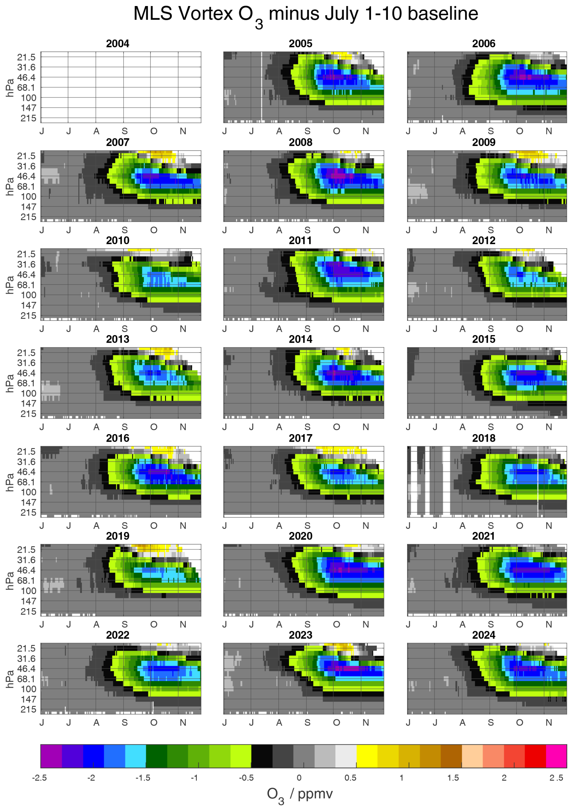
Figure 1 June to November vortex-average lower stratospheric ozone profiles over the range 215–21 hPa for 2005–2024. The respective 1–10 July average is subtracted for each year to remove interannual variability of early-winter (baseline) conditions. Partial 2004 is not included because MLS operations had not begun in July, so this baseline could not be calculated.

Figure 1 shows, for each year of MLS data from 2005 to 2024, time series from austral early winter through spring of weekly vortex-average differences from each year's respective 1–10 July baseline; only a minor amount of ozone loss generally occurs before July, as evidenced by the grey shades in June and July. In Fig. 2, we show the same vortex-average changes over the winter/spring for the (standard) WACCM simulation used in this work. The MLS data show that several years (2006, 2008, 2014, 2020, 2021, 2023, and 2024) have lower average values in October, after most of the chemical loss has occurred, especially in the lower portion of the vortex. Although WACCM generally shows slightly smaller ozone changes from baseline than MLS in September and October, the measured and modeled patterns of interannual variability are similar. The correlation between ozone losses and minimum temperatures in the lower stratospheric Antarctic vortex has been noted before (e.g., Kuttippurath et al., 2015; Roy et al., 2024). We discuss the correlation between temperature and ozone in the Antarctic vortex further below in the context of MLR fits to the MLS vortex-average ozone time series from 2005 to 2023.

Figure 2 Same as Fig. 1, but for the WACCM simulation and without year 2024.

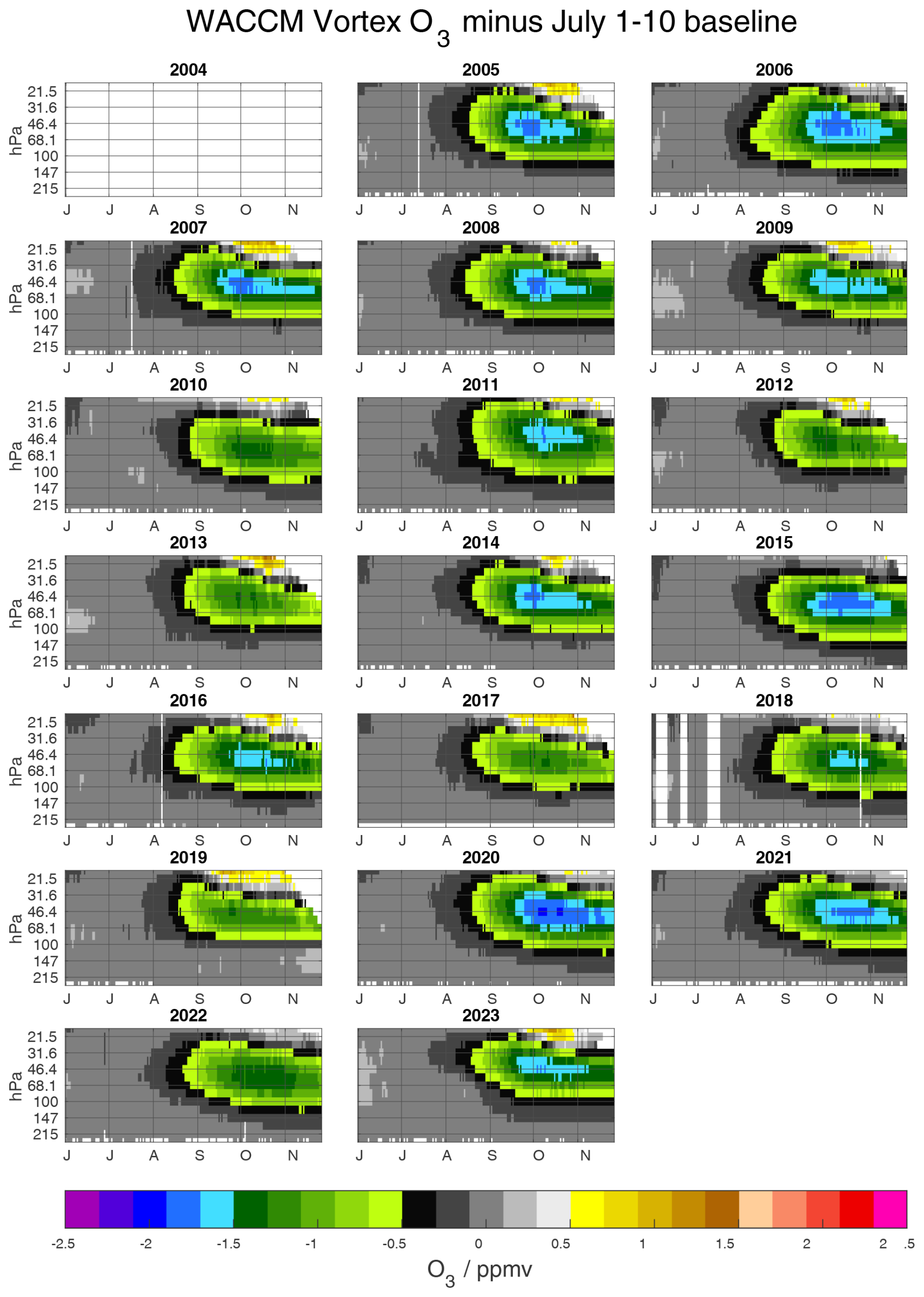
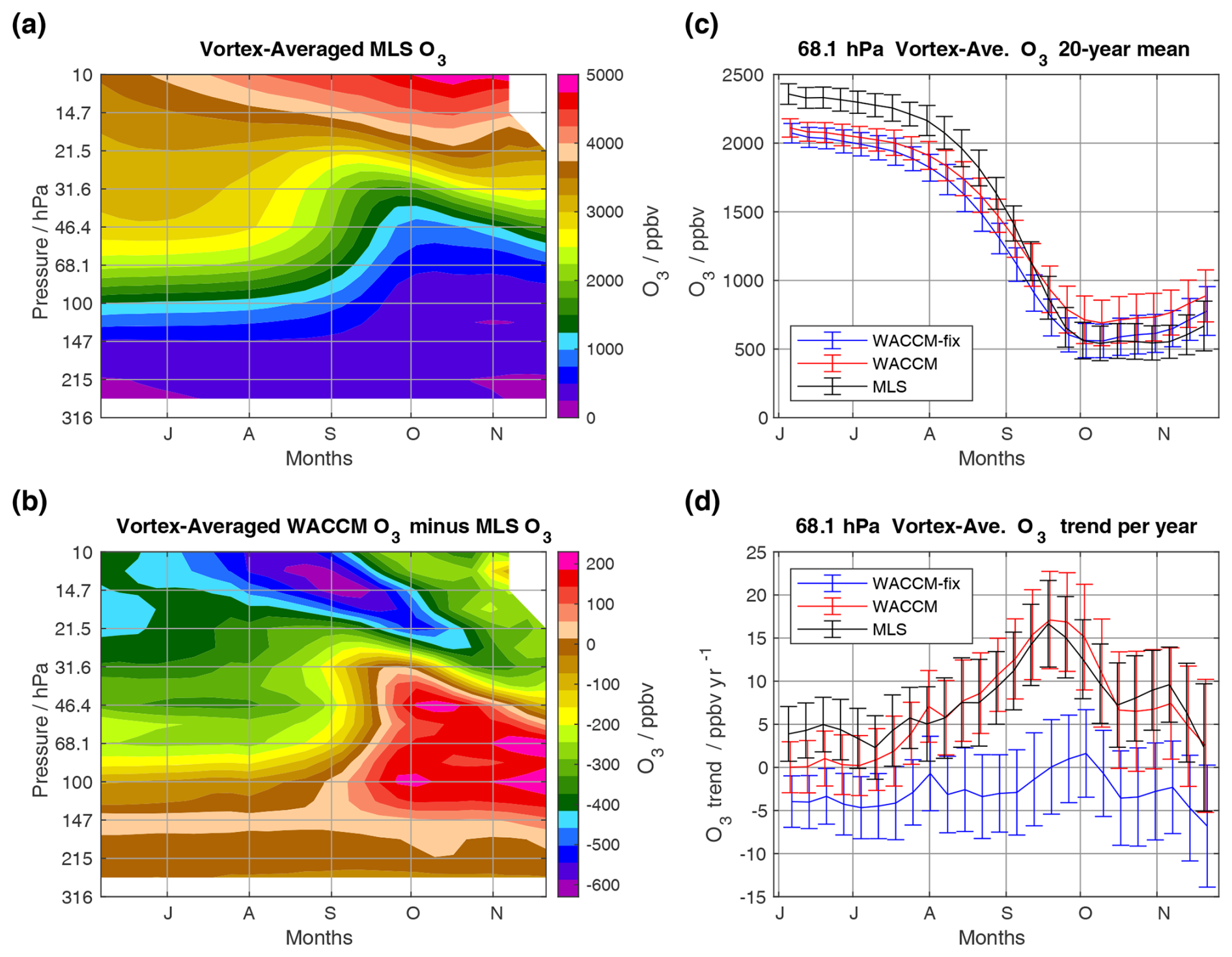
Figure 3 (a) Weekly mean Antarctic vortex-average ozone values from MLS in the lower stratosphere from early June to late November (weeks centered on day of year 157–325) for 2004 through 2023. (b) Average values from WACCM, as in panel (a), minus the MLS values shown in panel (a). (c) Example at 68 hPa of the mean ozone abundances for 2004–2023 from MLS, WACCM, and WACCM-fix-EESC (labelled “WACCM-fix”); the error bars represent the interannual standard deviation about the mean in these weekly average values over all the years. (d) Ozone trends (ppbv yr⁻¹) at 68 hPa obtained by fitting a simple linear trend to the yearly O₃ values contributing to each weekly average. Weeks prior to the start of MLS science data collection on 28 July 2004 are not included in these averages; thus results for the first eight weeks are 19-year averages and trends.

Figure 3a shows the climatological distribution of weekly average MLS ozone values from early-June to late-November for the period 2005–2023, and the difference between WACCM and MLS results is seen in Fig. 3b. The largest decreases in lower stratospheric Antarctic ozone occur during August and September (e.g., Chipperfield et al., 2022; Strahan and Douglass, 2018; Santee et al., 2024). Indeed, Fig. 3a shows that changes in MLS ozone occur mostly at pressures larger than 20 hPa after early to mid-August, with effects of downward transport visible in the contours at smaller pressures. The upper region is where the WACCM values are smaller than the MLS abundances, possibly because the multi-year average downward transport velocities are too small in the model; this conjecture seems to be qualitatively confirmed by a similar plot (not shown here) for N₂O, indicating that WACCM N₂O values are larger than MLS N₂O in the relevant height range. Some of the absolute differences may also come from systematic errors in the MLS data, since systematic uncertainties are as large as 5 %–15 % (Livesey et al., 2022). In the main region of chemical destruction after early September, the WACCM values tend to be larger than MLS data by about 100 ppbv, or ∼ 25 % (Fig. 3b). Figure 3c shows that WACCM O₃ mixing ratios at 68 hPa are ∼ 300 ppbv lower than those observed by MLS in June and July but end up on the higher end in October, implying somewhat smaller modeled seasonal ozone loss than is observed; a systematic bias between modeled and measured ozone would not produce this different behavior in the slope of the ozone change.

Figure 3d shows the slopes of linear fits to the time series of vortex-average ozone from MLS and both WACCM simulations at 68 hPa for 2004 to 2023. The trend estimates track well between MLS and WACCM, with positive trends typically between about 5 and 16 ppbv yr⁻¹, depending upon the date (weekly average) in winter or spring; the trends from MLS and WACCM both peak in mid-September. However, the trends obtained from the WACCM-fix-EESC simulation are consistent with a trend value of zero, as one might expect from such a fixed-EESC scenario. The seasonal patterns of changes in WACCM and MLS-derived trends are generally consistent throughout the winter/spring season from 147–14.7 hPa (not shown). The differences between WACCM and WACCM-fix-EESC trends are largest at 68.1 hPa and lose significance in this analysis by 14.7 hPa. At levels other than 68.1 hPa, there is generally more departure of the WACCM-fix-EESC trends from zero, likely reflecting the impact of changes in dynamics that are generally consistent among WACCM, WACCM-fix-EESC and MLS. More sophisticated ozone trend analyses are pursued in Sect. 3.2.

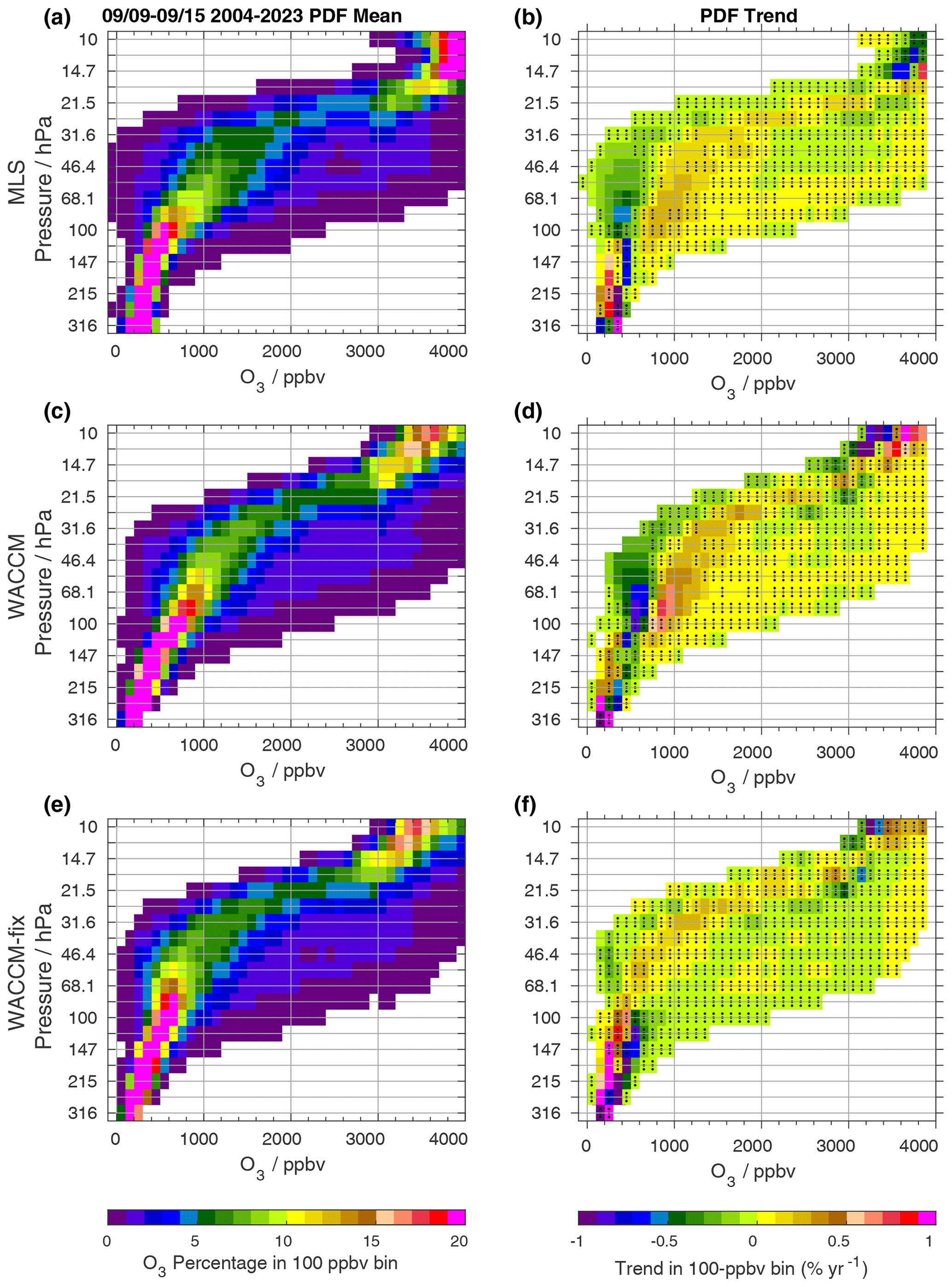
Figure 4 (a) A histogram of all MLS lower-stratospheric vortex O₃ observations from the week of 9–15 September for 2004–2023, normalized separately for each level, representing the underlying PDF. (b) PDF (histogram) trends shown are the slopes from linear fits within each bin to values from histograms prepared as in panel (a), but separately for each year. Bins without black stippling have trends that are larger in magnitude than the 1 uncertainty in the trend. Panels (c) and (d) are the same as panels (a) and (b), respectively, but for the WACCM simulation. Panels (e) and (f) are the same as panels (a) and (b), respectively, but for the WACCM-fix-EESC simulation.

Figure 4 depicts PDFs for vortex-average ozone (Fig. 4a, c, and e) and related trends in these distributions (Fig. 4b, d, and f) for the week centered on 12 September. Figure 4a, c and e all have sharply peaked distributions up to 83 hPa, with the broader distributions at 68–18 hPa reflecting larger spatial and/or interannual variability in lower stratospheric ozone. WACCM generally has slightly larger values than those of MLS at these levels. WACCM also lacks the near-zero values seen in the tail of the MLS PDF at 83–26 hPa, where MLS has observed some cases of early near-complete ozone depletion. At 68–46 hPa, the MLS single-observation precision is ∼ half of the width of a 100 ppmv histogram bin, so the MLS points near zero do not merely reflect random noise. The WACCM-fix-EESC distribution at these levels also has more of the lowest (100–200 ppbv) ozone values than the standard WACCM simulation, suggesting less recovery, as implied also by Fig. 3d; a larger value for EESC would indeed qualitatively account for such a difference between the two model simulations.

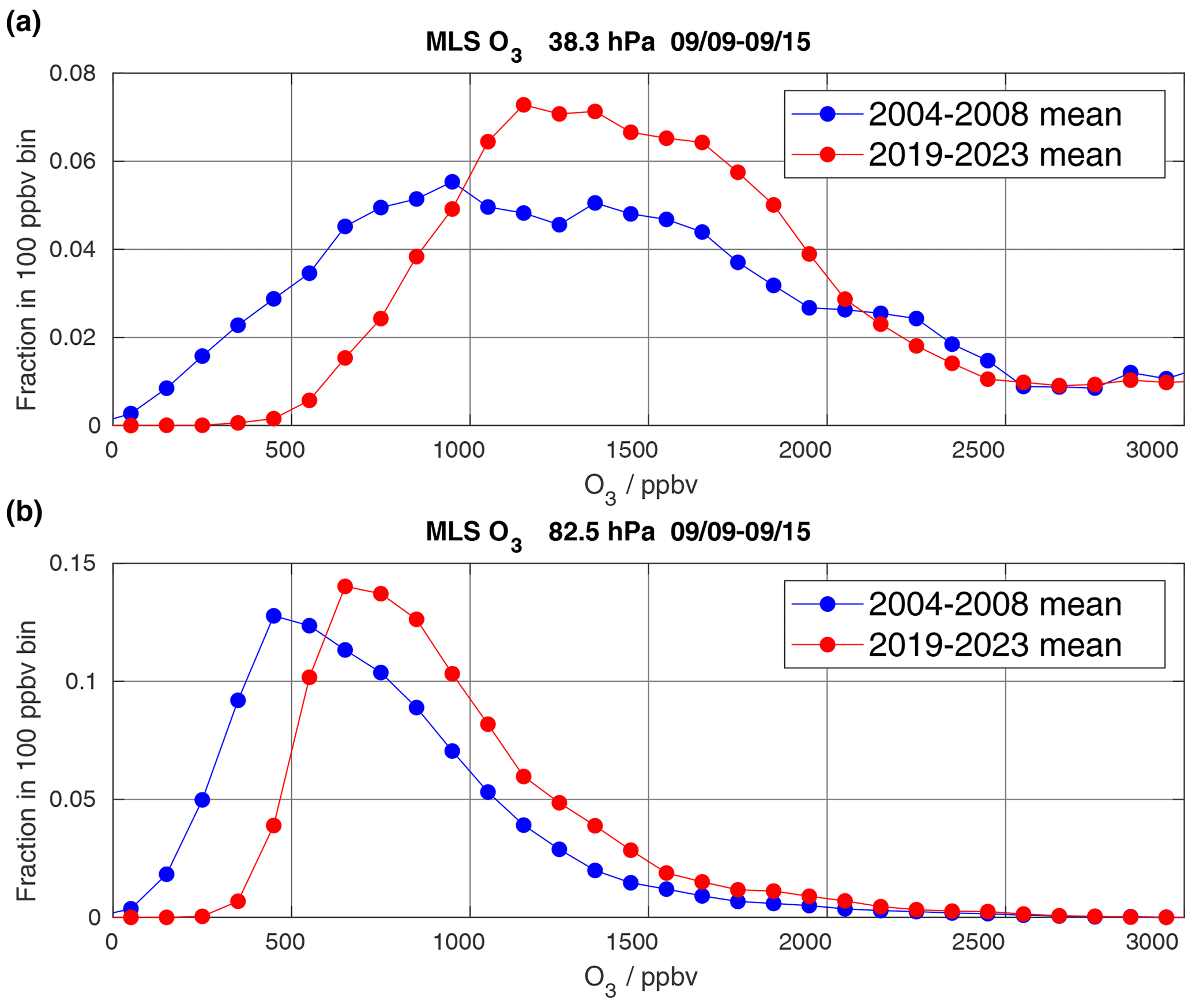
Figure 5 Fraction of the Antarctic vortex-average MLS ozone distributions in each 100 ppbv bin, for the week centered on 12 September for the periods 2004–2008 (blue) and 2019–2023 (red), at (a) 38.3 hPa and (b) 82.5 hPa.

The right side of Fig. 4 shows how the PDFs tend to change over time (from 2005 to 2023), with both MLS and WACCM showing shifts in the peaks of the distributions over the 20-year record, with fewer occurrences of values below 500 ppbv (green and blue areas on the left edge of Fig. 4b and d) and more at 800 ppbv and higher (brown areas of Fig. 4b and d). Bins without black stippling have trends with magnitudes more than twice the uncertainty in the fitted values. PDF trends for WACCM-fix-EESC in Fig. 4f show no shift from lower to higher values at 68–18 hPa, but rather an apparent tightening of the PDF, with brown sandwiched between green where Fig. 4b and d show such a shift. Figure 5 helps to visualize this shift by comparing the MLS PDFs at 38 and 82 hPa for a week in mid-September in two 5-year periods at the beginning (2004–2008, in blue) and end (2019–2023, in red) of the study period; in the later years, the peak of the distributions has clearly shifted towards larger abundances, and there are almost no ozone values below 500 ppbv. This result is consistent with work by Kuttippurath et al. (2018), who demonstrated decreasing saturation in lower stratospheric Antarctic ozone loss. However, if we consider a week in mid-October, results show only subtle changes in the MLS PDF trends (Fig. S1 in the Supplement); the ozone values are too small (and perturbed) during this period to allow for a robust trend detection.

Figure 6 Same as Fig. 3, but for HCl.

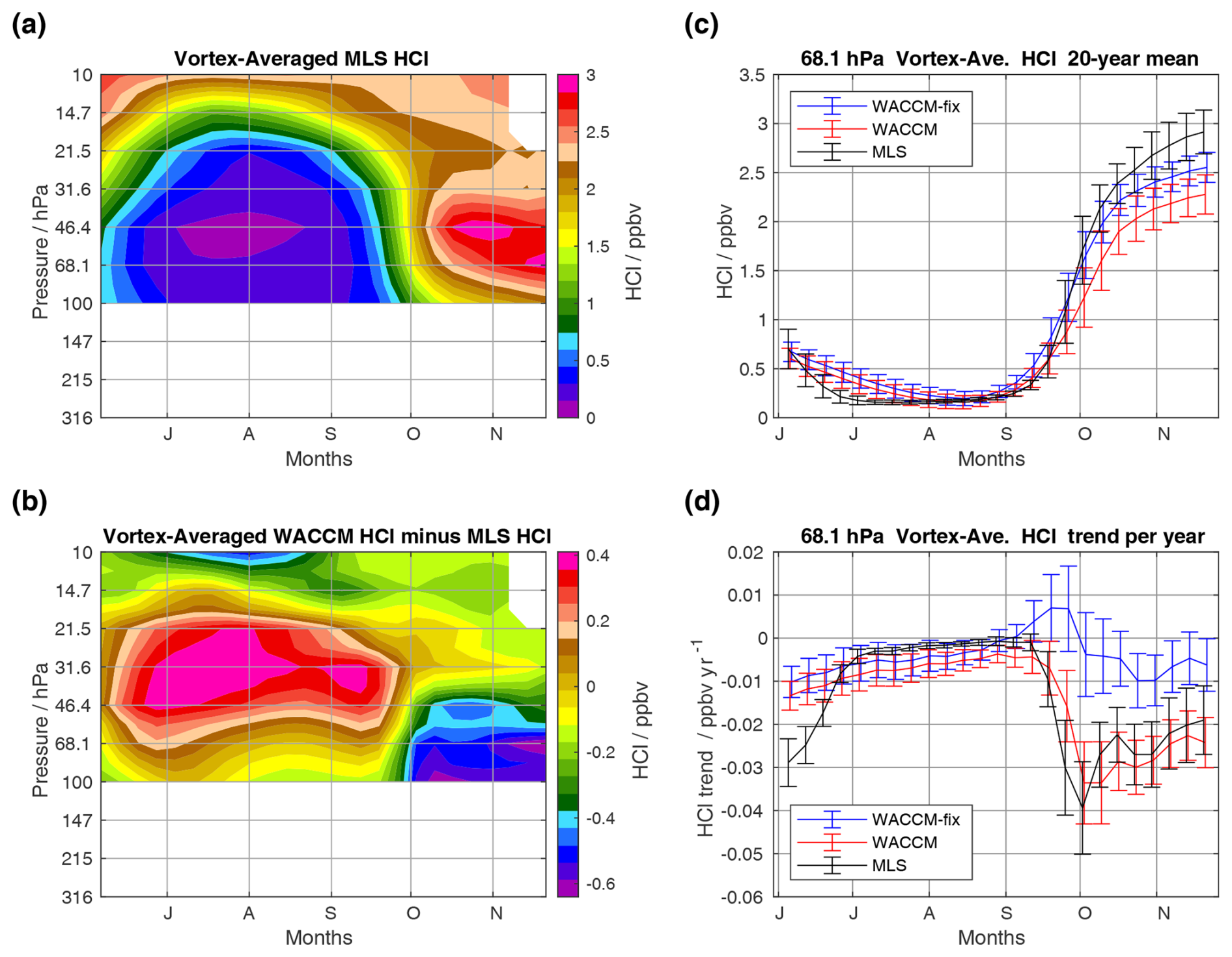
Figure 6 shows MLS HCl in the same format as for O₃ in Fig. 3. MLS shows highly depleted climatological HCl abundances during winter for pressures larger than 20 hPa, with a sharp increase at the end of September towards values between 2.5 and 3 ppbv in the spring (Fig. 6a). The differences in Fig. 6b indicate that WACCM has HCl values that are slightly larger in the winter but recover in the spring to mean values that are slightly smaller than those observed by MLS, as shown also at 68 hPa in Fig. 6c, where modeled HCl does not quite reach 2.5 ppbv at the end of November. The Antarctic early-winter discrepancy between HCl rates of decrease from models and from MLS has been addressed recently by Grooss et al. (2025), who point out that additional chemical mechanisms involving Cl₂O₂, HOOCl, and HOCl could resolve this issue, although there is a need for more laboratory validation regarding the reaction rates of these postulated mechanisms. The fact that WACCM has somewhat less HCl in the polar spring may in part reflect a total inorganic chlorine (Cly) value that is slightly low, possibly because of a deficit in very short-lived substances (VSLSs) and some inaccuracies in repartitioning during chlorine deactivation. Figure 6d shows linear trends of about −0.02 ppbv yr⁻¹ for vortex-average MLS HCl in late spring, when 68.1 hPa HCl abundances (∼ 2.8 ppbv) are comparable to mid-to-upper stratospheric HCl values. These trends correspond to about −0.7 % yr⁻¹, which is somewhat larger than global trends (since the turn of the century) in upper stratospheric HCl of about −0.3 % yr⁻¹ to −0.5 % yr⁻¹ (WMO, 2022). In contrast, the WACCM-fix-EESC simulation leads to HCl trend results that are consistent with zero trend, as one would expect.

Figure 7 Same as Fig. 3, but for HNO₃.

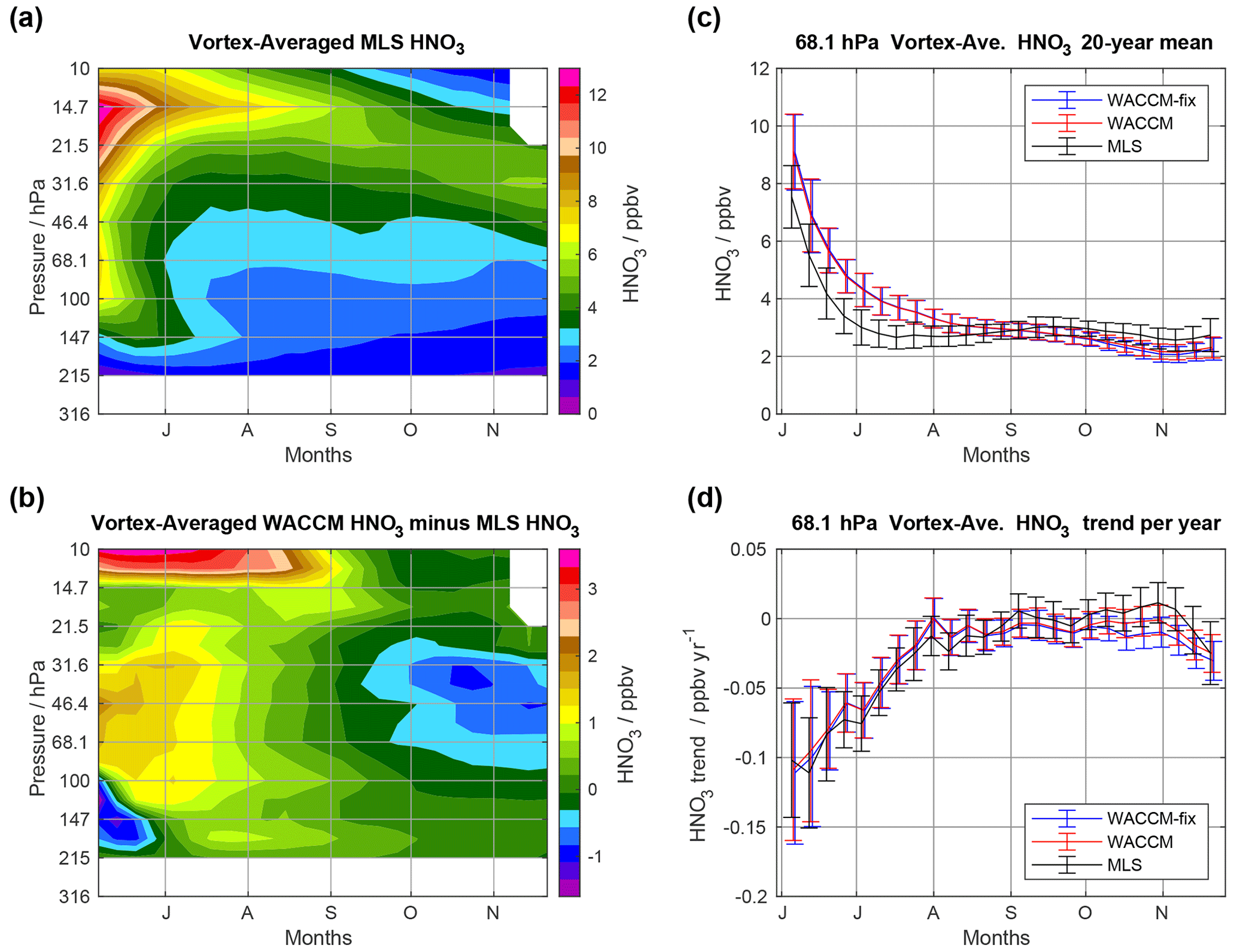
Figure 7 is analogous to Figs. 3 and 6, but for modeled and observed HNO₃. Strong depletion of gaseous HNO₃ is observed in the climatology from MLS (Fig. 7a), with the WACCM simulation (Fig. 7b) showing slightly larger values than the MLS abundances in early winter and slightly lower values in the spring. As mentioned in Sect. 2.2, this WACCM fit to Antarctic HNO₃observations is clearly better than that in previous simulations from WACCM, following improvements in the modeled heterogeneous chemical processing scheme. In Fig. 7d, the MLS and modeled linear trends in HNO₃ from 2005 to 2023 all agree very well, with near-zero trend for most months. During June and July, a negative trend is apparent in MLS data as well as in the model simulations. Investigation of the underlying cause of these apparent trends in early-winter HNO₃ is beyond the scope of this study.

3.2 Further analyses of trends in Antarctic vortex ozone

3.2.1 MLR analyses of vortex-average ozone trends

Here, we use 7 d means of Antarctic vortex-average ozone abundances for 2005–2023 to perform multivariate linear regression analyses to produce better fits to the time series and reduce the error bars compared to a fit with only a linear trend term (and a constant term). We apply the same analyses to both model simulations.

The main regression model used here has two sets of periodic functions, both described by sine and cosine terms, with period 1 and period 2 representing, respectively, a short-term and a decadal-type component. Our standard run has a 2.5-year periodicity for period 1, since we observe (see further below) that most Antarctic time series exhibit short-term variability. Moreover, the quasi-biennial oscillation (QBO) is a well-studied phenomenon in the Earth's stratosphere (e.g., Baldwin et al., 2001; Anstey et al., 2022) that can be represented by such a periodicity; there is evidence of QBO influence on Antarctic temperature and inorganic chlorine (and thus ozone) over Antarctica (Strahan et al., 2014; Strahan and Douglass, 2018). We should note that using a 2- or 3-year periodicity for period 1, rather than 2.5 years, does not lead to major changes in terms of our trend results, given the typical trend uncertainties. We have also varied period 2 (see further below), but our standard retrieval uses a value of 11 years, which can represent solar cycle variability, even if this may not be the main cause of decadal-type variability in Antarctic ozone. The other terms in the MLR analysis are a constant and a linear (trend) term.

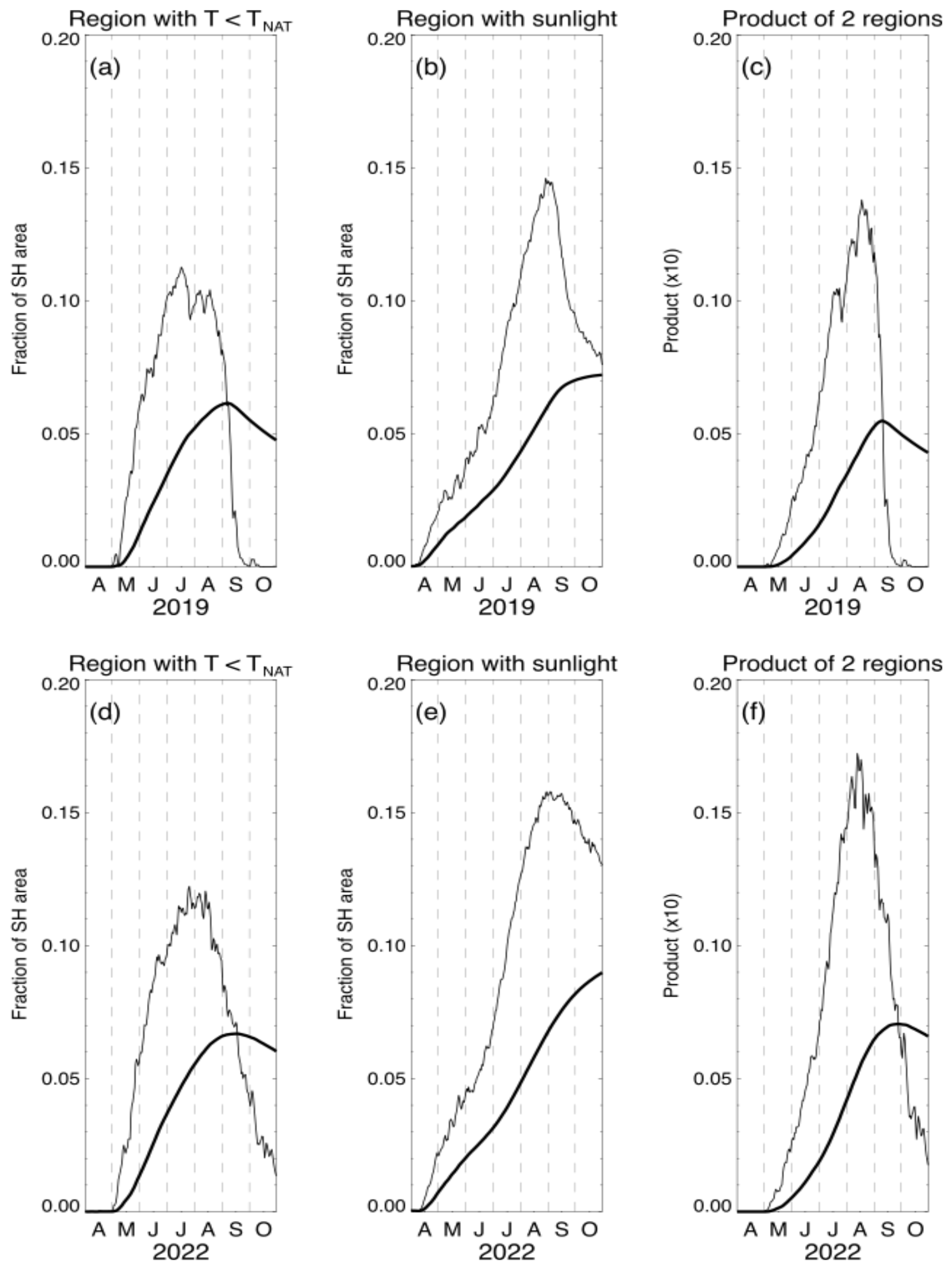
Figure 8 The lower stratospheric layer-average Antarctic vortex area with T < T_NAT for (a) 2019 and (d) 2022; the lower stratospheric layer-average Antarctic vortex area exposed to sunlight for (b) 2019 and (e) 2022; and the product (multiplied by 10) of these two layer-average areas for (c) 2019 and (f) 2022. Layer averages are calculated over potential temperature levels from 330 to 620 K. The thin lines depict daily quantities, whereas the thick lines are time-averaged values of these quantities through each day of the year, from 1 April. The layer-average area diagnostics are expressed as a fraction of the total Southern Hemisphere (SH) area.

Also, we use a proxy term tied to the region within the vortex with temperatures allowing the possible existence of polar stratospheric clouds (PSCs). The volume (VPSC) of air that is exposed to temperatures below T_NAT, the threshold for existence of nitric acid trihydrate (NAT) PSCs, has been shown to be well correlated with springtime ozone loss in the polar vortices (e.g., Rex et al., 2004; Tilmes et al., 2004). Although it is known that liquid-phase particles play a large role in the destruction of polar ozone, the T_NAT threshold is often used as a first-order estimate of the conditions necessary for significant chemical ozone destruction inside the polar vortex. To describe the proxy we use for the VPSC term, we show in Fig. 8 the area with temperatures below T_NAT and the area of the vortex exposed to sunlight (Lawrence et al., 2015, 2018), since sunlight is required for the photochemical processes involved in Antarctic vortex ozone destruction (see the review by Solomon, 1999). In Fig. 8a and d, the areas (expressed as a fraction of the SH hemisphere area) from different potential temperature levels (from 330 to 620 K) are averaged to obtain a lower stratospheric layer-average area, which is akin to a summation (or volume, VPSC). The second variable represents the lower stratospheric layer-average sunlit vortex area (also as a fraction of the SH hemisphere area) , which is then multiplied by VPSC. This product (Fig. 8, right-hand panels) is used as a proxy term (labeled VPSC_sun in the fitting function below) for our MLR analysis of ozone vortex-average abundances. The 2019 vortex was significantly perturbed by a September sudden stratospheric warming event, leading to an anomalously small Antarctic vortex and column ozone destruction (e.g., Wargan et al., 2020; Roy et al., 2024). Figure 8 shows that the lower stratospheric layer-average vortex area with temperatures below T_NAT drops much faster in 2019 (Fig. 8a) than in a representative year like 2022 (see Fig. 8d); this also affects the time-averaged (mean from 1 April to date) layer-average diagnostic values (thick lines) in September and October, as well as the final proxy values in Fig. 8c and f, even if the averaged effect is dampened compared to the daily values (thin lines).

The MLR time series function to be fitted for coefficients a, b, c_n, d_n, and f has the following form:

$$\begin{array}{}\text{(1)}& \begin{array}{rl}y\left(t\right)=& a+b\left(t-t_{\mathrm{m}}\right)+\sum _n\left(c_n\sin \mathrm{2}\mathit{\pi }t/P_n\right.\\ & \left.+d_n\cos \mathrm{2}\mathit{\pi }t/P_n\right)+f{\mathrm{VPSC}}_{\mathrm{sun}}\left(t\right)\end{array}\end{array}$$

with the yearly time series values expressed by time (t); t_m refers to the series mid-point, and the linear trend term is coefficient b. The sine and cosine functions provide for periodic variations with periods P_n. As mentioned above, we use two periods in the MLR equation – a short-term (QBO-type) period (P₁) and a longer-term (decadal-type) period (P₂); in a sensitivity study discussed later, we add a term relating to the Antarctic Oscillation.

In Fig. 9, we show examples of the year-to-year relative changes in the lower stratospheric VPSC_sun proxy from 2005–2023 for the week centered on 19 September, along with the vortex-average ozone abundances from MLS for that week. As indicated by the values of the correlation coefficient (R), there is an anti-correlation between mean ozone and the VPSC_sun proxy; for example, the 2019 vortex, with its larger-than-usual ozone values in late September, shows a positive peak, whereas the proxy indicates a low value for that year. An expanded view of this correlation coefficient versus pressure level for various weeks in September and October is provided in Fig. 10, which shows that the anti-correlation between ozone and VPSC_sun grows between early September and late October, when the cumulative impact of chemical ozone destruction peaks. To first order, we expect that a polar vortex winter/spring with lower-than-average temperatures will lead to more chemical processing and larger chemical ozone destruction, with relatively smaller vortex-average ozone values in the spring.

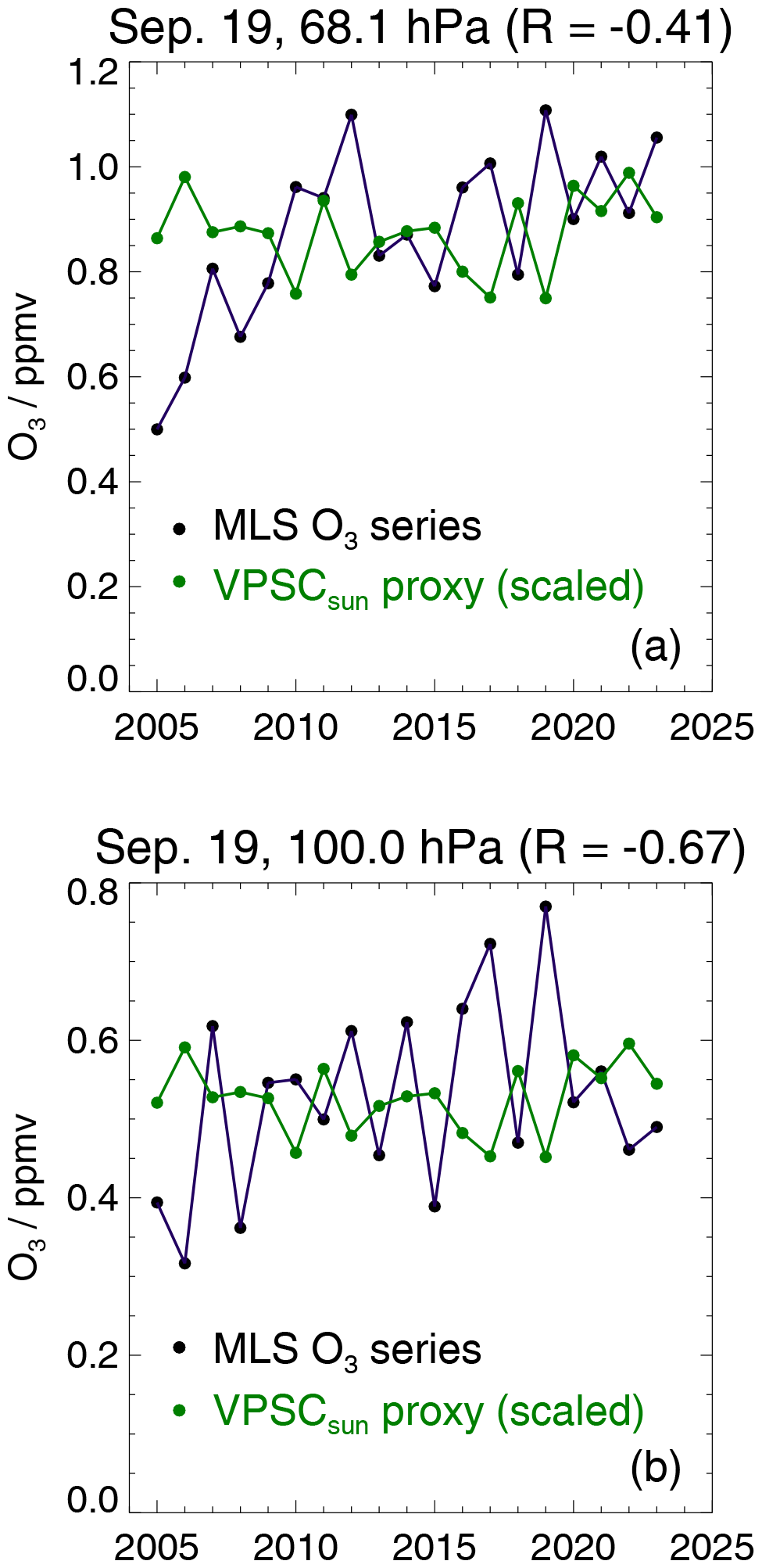
Figure 9 Vortex-average Antarctic ozone variations from MLS (black) over 2005–2023 for the week centered on 19 September at (a) 68 hPa and (b) 100 hPa. The green lines are a scaled version of the variability in the VPSC_sun proxy term described in the text (in relation to Fig. 8); the scaling (using the average ozone value over the years divided by the average relative change in the proxy) is applied here to show the relative changes in this proxy from year to year on the same scale as the ozone ranges in each panel.

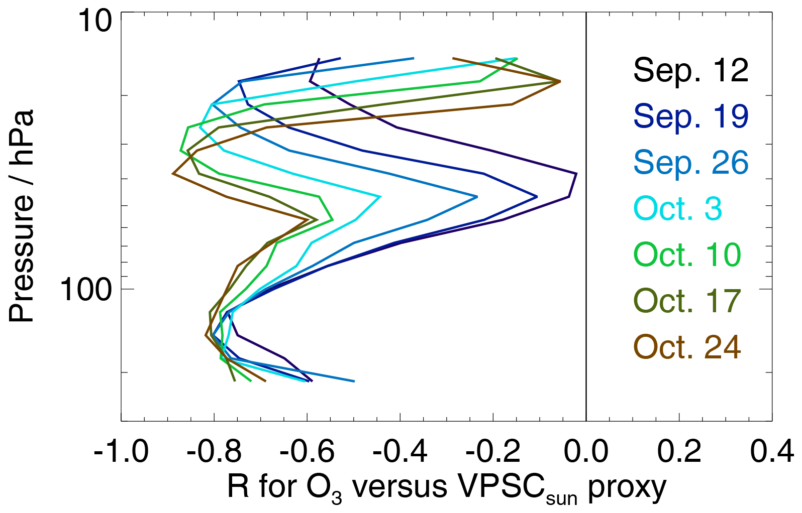
Figure 10 An expanded view of the correlation coefficient (R) between the ozone vortex-average time series and the lower stratospheric VPSC_sun proxy described in the text and in Fig. 8. Results are shown as a function of pressure for each of the September and October weeks considered here, as labeled on the right side of this plot.

In Fig. S2, we show that use of longer periods (9 to 11 years) for P₂ enables the MLR analysis to explain a larger fraction of the variance at pressures between 56 and 100 hPa, in comparison to 4- to 8-year periods; choices of 9, 10, or 11 years do not lead to very different correlations. We have chosen to use 11 years for our standard MLR retrievals. The 11-year solar cycle can impact ozone through standard photochemistry (related to solar ultraviolet flux) or energetic particle precipitation (EPP) (e.g., Gordon et al., 2021). EPP can have a direct impact on ozone in the upper stratosphere and mesosphere, as well as indirect effects from downward transport of nitrogen oxides to lower altitudes, although the likely long-term impact of EPP on lower stratospheric Antarctic ozone is difficult to ascertain (Maliniemi et al., 2022). However, we note that the phase of the solar cycle itself does not agree with the typical phase of the proxy term that we derive from the MLR fits. The correlation between the 11-year fitted component and the solar cycle variation itself changes with pressure, with a range of positive, negative, or near-zero correlations; elucidating a causal relationship would require modeling that is beyond the scope of this paper. Transport variability is another factor that can modulate Antarctic vortex ozone abundances (e.g., Kessenich et al., 2023). More generally, there is evidence for multi-year variability and hemisphere-dependent changes in HCl (Mahieu et al., 2014) and HNO₃ (Strahan et al., 2020), with changes in the circulation invoked as a likely driver; these variations could also influence the variability in Antarctic ozone. Some transport-related variability is included in the VPSC_sun proxy through the influence of temperatures and vortex area. However, we focus on winter/early spring periods when chlorine and bromine chemical effects are at their strongest over the well-isolated lower stratospheric Antarctic vortex.

We show in Fig. S3 the same plots as in Fig. S2, but for P₁, the 2.5-year period we have used in our standard MLR fits. As one might expect, the fraction of variance explained by the short-term period does not have sensitivity to the value of P₂. This is shown mainly to contrast the R² values from P₁ with those from P₂. For 56 and 68 hPa, the P₂ term explains more of the variance in the ozone time series, whereas the short-term period explains more of the variance at 82 and 100 hPa.

We have applied the MLR analysis described above, including the VPSC_sun variability term, to the MLS-derived Antarctic vortex-average values from different September and October weeks over 2005–2023. Examples of the ozone time series and the fits are shown in Fig. 11 at 68 and 100 hPa for the week centered on 19 September. Both the linear component (slope of the fit) and the full fit to the time series are shown; as expected, much better results are obtained with the full fit. Figure 12 compares the overall results at 68 hPa for the MLR-based MLS vortex-average ozone trends in September and October to the trends obtained from simple linear regression. Although the trends themselves do not change very much, the trend error bars are significantly reduced in the MLR case (Fig. 11a); on average, there is a 20 %–25 % reduction in the error bars, with a reduction of ∼ 40 % at 121 hPa and ∼ 10 % at 46 hPa. In Fig. 12b and c, we also show how diagnostics of the fit quality change between these two regression methods. The MLR fits, in comparison to simple linear trend analysis, yield much larger correlation coefficients (0.8 to 0.95 rather than 0.4 to 0.5) and smaller RMS residuals (by a factor of 30 %–50 %). Figure S4 provides the same information for 100 hPa, with similarly improved results for the MLR case.

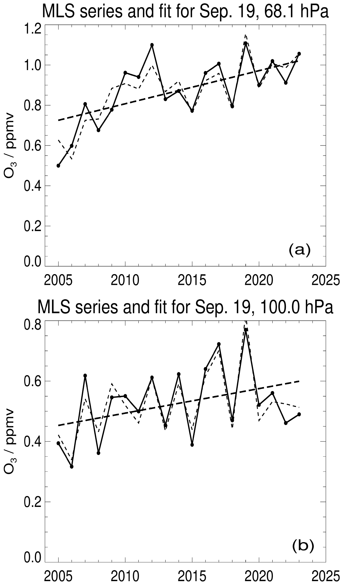
Figure 11 Examples of MLR fits to the MLS vortex-average ozone time series at (a) 68 hPa and (b) 100 hPa for the week centered on 19 September. The MLS ozone averages are given by the solid line, the ozone trend (slope component of the MLR fit) is shown by the thick dashed line, and the thin dashed line gives the full fit from the MLR analysis.

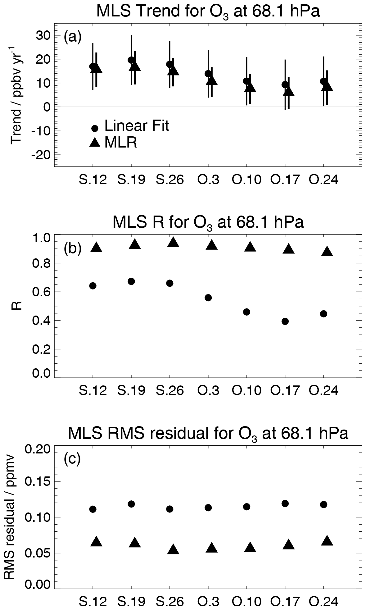
Figure 12 Results at 68 hPa for (a) the trends in MLS vortex-average ozone over Antarctica, (b) the correlation coefficients between the fits and the MLS O₃ series and (c) the RMS residuals for these fits, as a function of weeks in September and October (centered on 12 September, labeled S.12, to 24 October, labeled O.24). The filled circles and filled triangles represent results from a simple linear fit and MLR, respectively, for 2005–2023. Trend error bars in panel (a) represent 2σ.

Figure 13 shows the MLR-based trends for 2005–2023 at 46, 68, and 100 hPa for MLS and the two WACCM simulations of Antarctic vortex ozone (sampled following the MLS viewing pattern). We find that some of these lower stratospheric Antarctic vortex-average ozone trends in September and October are significantly different from zero (taken here to mean further from zero than the 2σ error bar) for pressures larger than 50 hPa. For example, the mid-September to early October MLS ozone trends (black points) are significantly different from zero at 68 and 100 hPa. Typical September MLS trends are ∼ 15 ppbv yr⁻¹ at 68 hPa and ∼ 7 ppbv yr⁻¹ at 100 hPa, while October trends at these two levels are mostly between zero and 10 ppbv yr⁻¹. The WACCM simulation (red points) generally matches the MLS results quite well, although the error bars are slightly larger. Also, as for MLS, most of the WACCM trends in October are not significantly different from zero. The WACCM-fix-EESC simulation (blue points) yields lower stratospheric ozone trends that are consistent with zero, as one might expect from a fixed-EESC scheme. We provide in Figs. 14 and 15, respectively, the correlation coefficients and the RMS residuals, as introduced in Fig. 12 for MLS, for the results from MLS, WACCM, and WACCM-fix-EESC at 46, 68, and 100 hPa. At 68 and 100 hPa, the R values typically lie between 0.8 and 0.95 for MLS and WACCM, with slightly lower values for WACCM-fix-EESC. Correlation coefficients are somewhat lower in general at 46 hPa, a region where the trends are most often found to be not significant. The variation of the WACCM RMS residuals as a function of pressure follows that obtained for MLS; there is not much variation in these, or in the R values, as a function of the September and October dates.

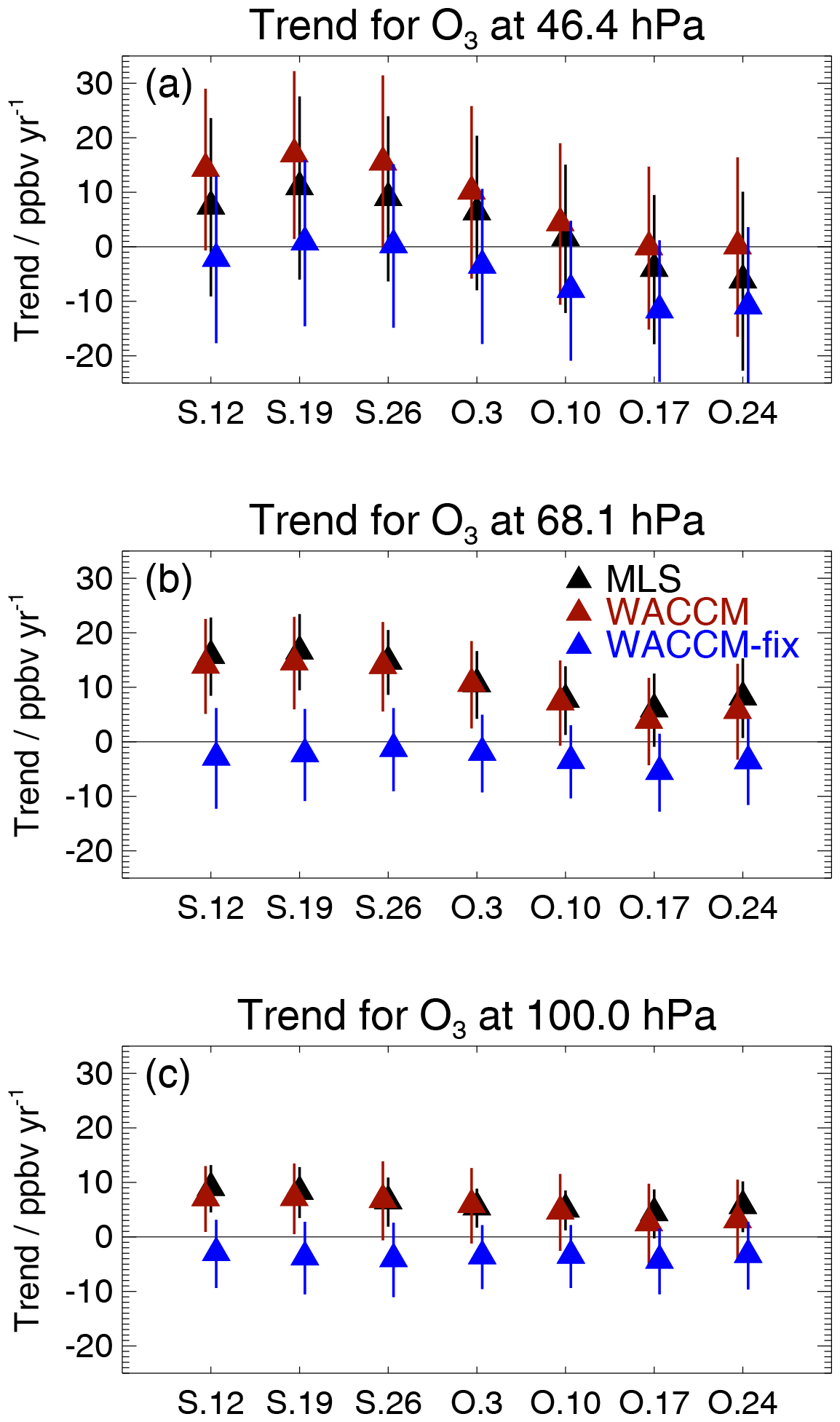
Figure 13 A comparison of the vortex-average trends for 2005–2023 based on MLR analyses from MLS, WACCM, and WACCM-fix-EESC (labeled WACCM-fix) for the weeks from 12 September through 24 October for (a) 46 hPa, (b) 68 hPa, and (c) 100 hPa.

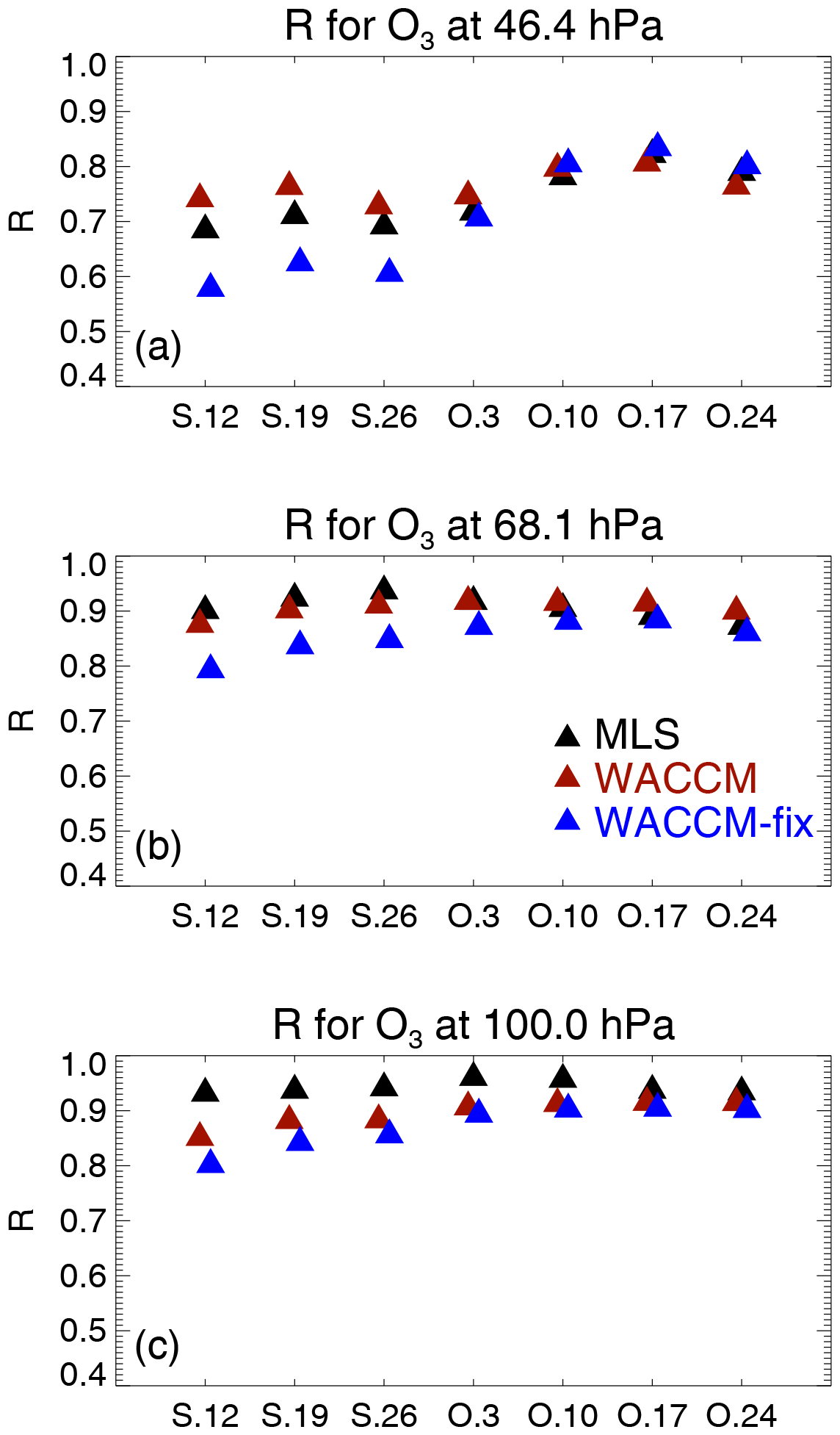
Figure 14 Same as Fig. 13, but for the correlation coefficients (R) calculated for the MLR fits to the vortex-average ozone time series.

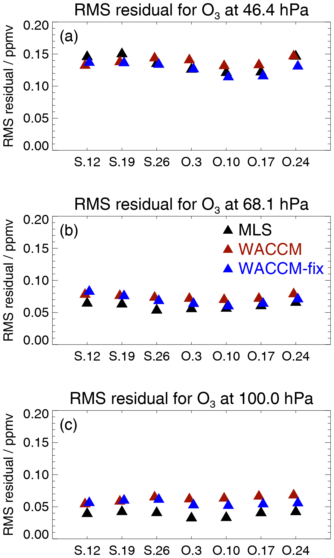
Figure 15 Same as Fig. 13, but for the RMS residuals of the MLR fits to the vortex-average ozone time series.

We also provide another way of roughly estimating the changes that occur in winter/spring inside the Antarctic vortex, by taking the differences (ΔO₃) between the vortex-average ozone values in September or October and the mean vortex ozone values from the first week in July, before substantial chemical ozone loss has occurred, especially in the lower stratosphere, where the positive trends are most significant. This approach is commonly employed to partially mitigate the effects on ozone arising from transport-related variability. For example, Strahan et al. (2019) used this methodology and noted that the majority of ozone loss occurs after early July. Figure 16 gives trends in the lower stratosphere for the MLS, WACCM, and WACCM-fix-EESC cases; values are close to and consistent with the results in Fig. 13, which considers the actual ozone values rather than differences from an early winter baseline.

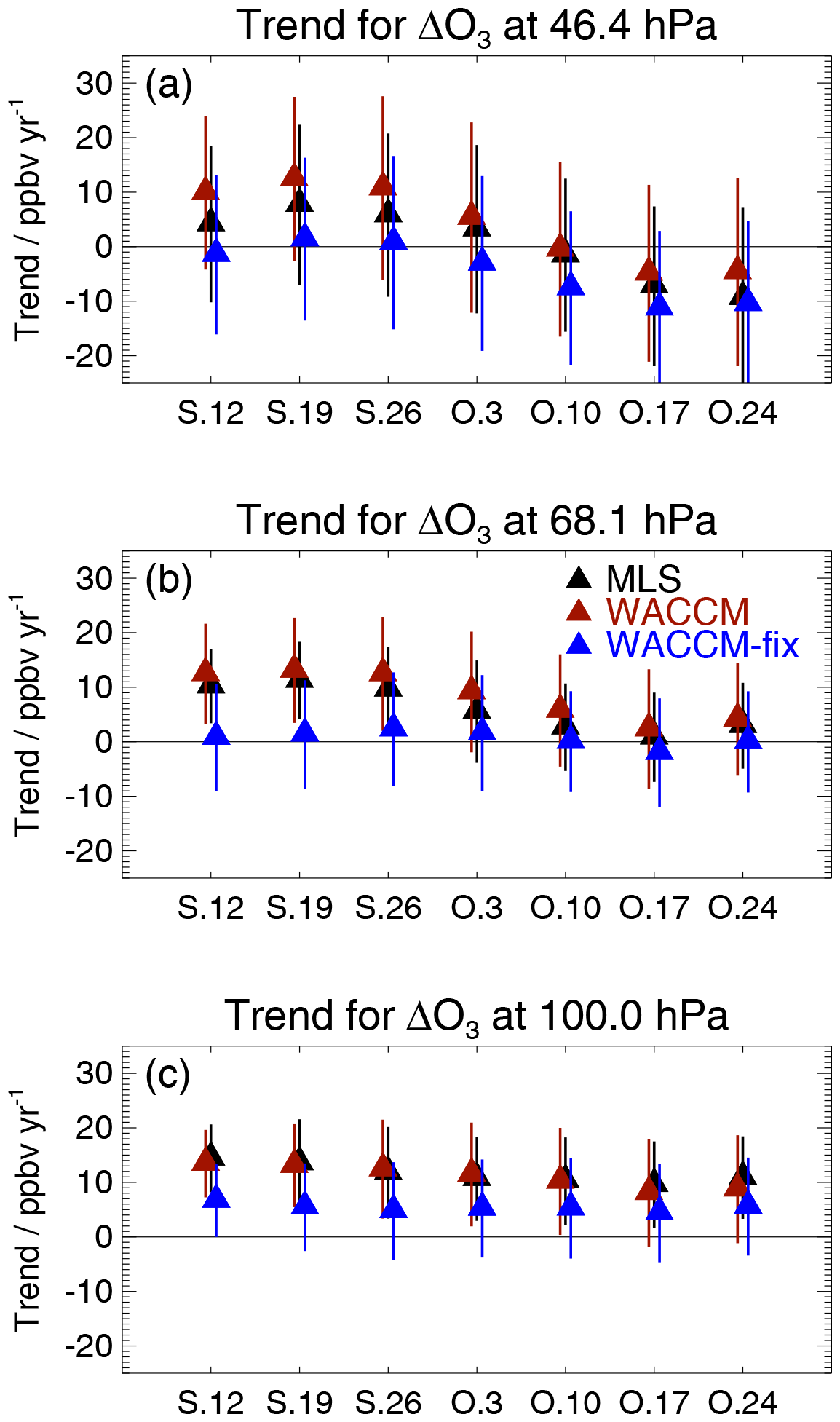
Figure 16 Same as Fig. 13, but for MLR analysis results from time series of vortex-average ozone in the first week of July subtracted from the September and October weekly average ozone values; we refer to this methodology as ΔO₃ analyses rather than O₃ analyses.

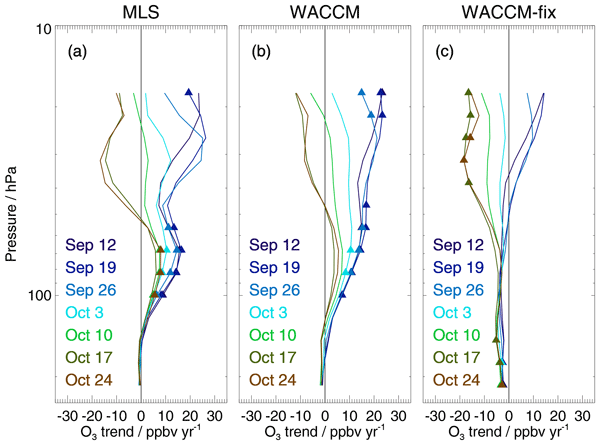
Figure 17 provides a summary of the MLS, WACCM, and WACCM-fix-EESC Antarctic vortex-average ozone trend profiles in the lower stratosphere for each of the September and October weeks that we analyzed, with triangles marking trends found to be significantly different from zero. The trends for MLS and WACCM that are significantly different from zero are all positive, with September trends of order 5–15 ppbv yr⁻¹ peaking at 68 hPa and with somewhat smaller trends (5–10 ppbv yr⁻¹) in October, which usually brings more perturbed conditions as the vortex weakens.

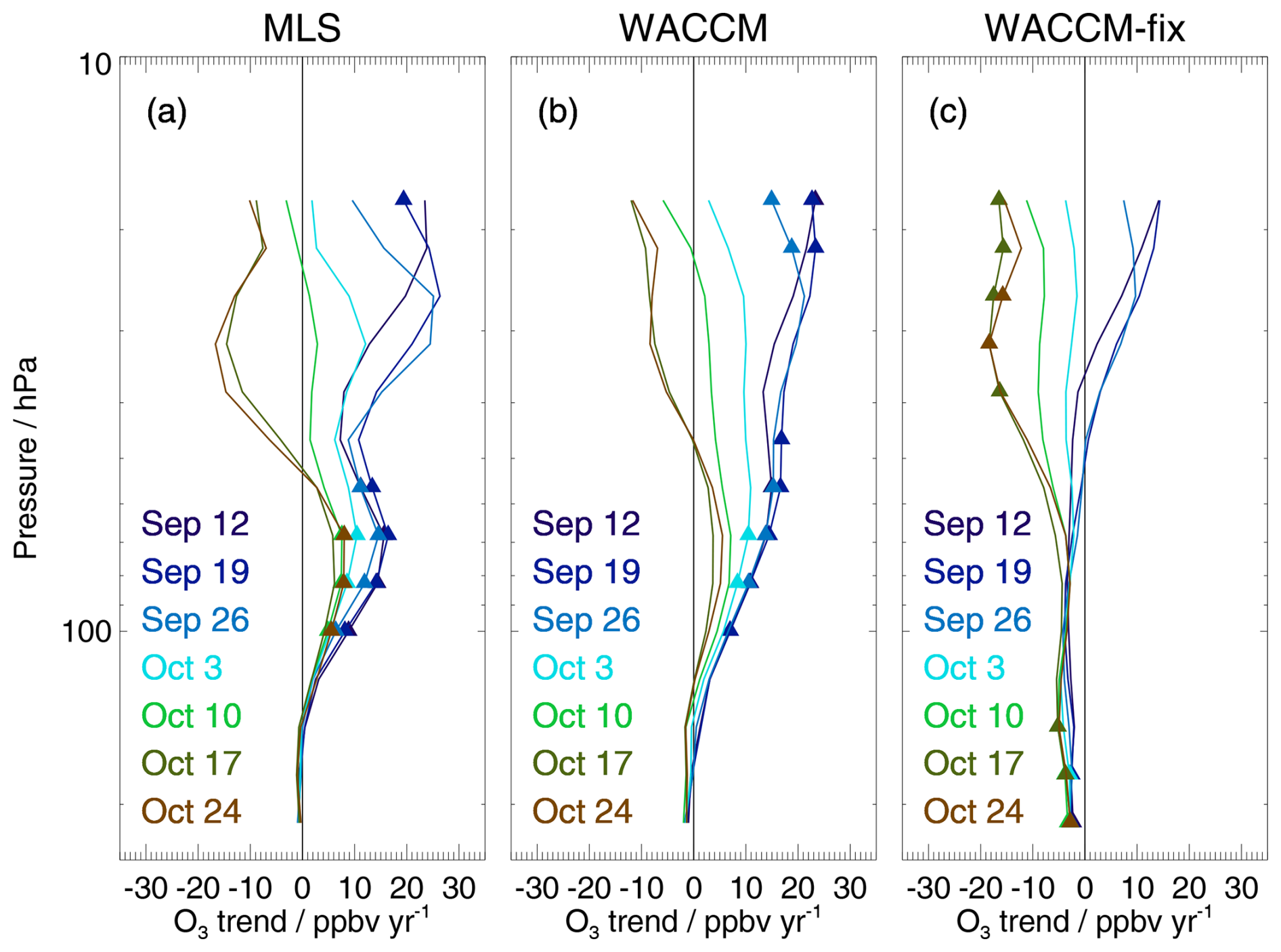
Figure 17 Trends in Antarctic vortex-average ozone from (a) MLS, (b) WACCM, and (c) WACCM-fix-EESC (labeled WACCM-fix) based on MLR analyses from 2005 to 2023. The different curves depict weekly averages centered on the dates shown. The trends that exhibit statistical significance (based on our definition at the 2σ level) are marked by triangles.

For pressures larger than 50 hPa, the analyses of 75–82° S zonal mean MLS daily data from 2004 to 2022 by Kessenich et al. (2023) also show some significant positive trends of 10–20 ppbv yr⁻¹ in September. Similarly, positive (and significant) September trends of 15–30 ppbv yr⁻¹ are obtained for 2001–2023 in this pressure range by He et al. (2026), who recently analyzed zonal mean values in the broader 60–90° S region from the chemistry transport model TOMCAT. Wang et al. (2025) obtained significant September vortex-average trends in MLS ozone of 15–20 ppbv yr⁻¹ in the same pressure range for a shorter time period (2005–2018), but this trend would probably have been slightly smaller if the period under consideration had included more of the recent years with a colder than usual lower stratospheric vortex.

For pressures less than 50 hPa, significant mean September trend values in vortex-average ozone obtained by Wang et al. (2025) peak at ∼ 40 ppbv yr⁻¹ (near 20–30 hPa). These trends are significantly larger than our weekly mean MLS September trend results at those pressures (with trends peaking at ∼ 20 ppbv yr⁻¹ but generally not significant). This apparent discrepancy in derived ozone trends is likely largely attributable to differences in the analysis periods used. Also, the 20–30 hPa (∼ 540–620 K, ∼ 22–25 km) layer, which lies just above the region of strongest chemical processing in the heart of the ozone hole, is subject to large interannual variability in the relative interplay between dynamical and chemical effects in September and October. Thus, as illustrated in Fig. S5, it is particularly sensitive to the interval chosen (both start and end dates) for ozone trend estimation; trend uncertainties are also large in this region. At pressures smaller than 50 hPa, the WACCM simulation with fixed EESC gives results that scatter about zero and are generally not significantly different from zero, although there are a few significantly negative values in late October that might be associated with transport-related changes during the more dynamically perturbed conditions. Indeed, even the MLS (Fig. 17a) and WACCM (Fig. 17b) results show more variability in the mid-stratosphere, with some non-significant negative late-October trend values. For this region, Kessenich et al. (2023) obtained significant (and large) negative October trends, mostly in the range of −50 to −100 ppbv yr⁻¹. These authors have argued that negative trends in October could be the result of a slight delay in the ozone hole spring break up as a function of year. The TOMCAT trends obtained by He et al. (2026) in this pressure range are also negative in October, with values between about −30 and −80 ppbv yr⁻¹; the earlier starting year (2021) used by these authors could lead to some differences in results. Also, Wang et al. (2025) point out that ozone trends over Antarctica are shifted towards zero or more negative trends if zonal-mean polar ozone data are used rather than vortex averages.

In addition, we tested a regression including a term for the variability that arises at high southern latitudes in connection with the Antarctic Oscillation (AAO), which characterizes atmospheric mass and pressure changes between the southern midlatitudes and the Antarctic region (e.g., Gong and Wang, 1999). More information on the estimation of the AAO index can be found at https://www.cpc.ncep.noaa.gov/ (last access: 13 August 2026). The AAO appears to have several multi-year variability components, including a periodicity of about 6 years and other longer-term periodicities (Zhang et al., 2010). If we add the winter/spring average AAO index changes as a function of year to the previously described regression fits, the results are similar to and consistent with the MLR results for MLS, WACCM, and WACCM-fix-EESC shown above, both in terms of trends and their corresponding error bars (Fig. S6). The addition of such an AAO proxy does not substantially change the total explained variance or the RMS residuals of the fits (not shown).

Finally, we comment briefly on the upper stratospheric Antarctic vortex from our simple linear trend analyses, as MLR analyses including a VPSC proxy are not appropriate for that region. Essentially no significant upper stratospheric trends are found for the three weeks in September considered (Fig. S7). The October trends (not shown) are most often not significant in the lower stratosphere and have even more scatter in the upper stratosphere, where MLS and both WACCM simulations show a negative but generally not significant trend. Dynamical changes may be the reason for this behavior, further analysis of which is beyond the scope of this study.

3.2.2 Ozone loss trends from Match analyses of MLS data

We now turn to an ozone trend analysis that focuses more specifically on the winter/spring chemical ozone losses inside the Antarctic vortex and better accounts for transport-related changes, including descent across pressure surfaces or leakage into or out of the vortex. The so-called Match technique was pioneered by von der Gathen et al. (1995), who used multiple ozonesonde profiles within the Arctic vortex to quantify chemical ozone loss. This methodology has been applied (e.g., Livesey et al., 2015; Santee et al., 2024) to Aura MLS ozone within the polar winter vortices; chemical ozone loss is estimated by tracking a multitude of observed parcels using trajectory calculations along potential temperature surfaces and matching the parcels to subsequent MLS measurements during winter and spring.

Figure S8 shows daily cumulative ozone losses for each year from 2005 to 2023 from Match results inside the Antarctic vortex during May to October at four different potential temperature levels between 350 and 700 K; given that noise in these calculations leads to positive and negative changes in May and June, we focus on the net negative changes (chemical losses), which typically occur after 1 July. In October, there can be a slight turnaround in the cumulative changes, as the vortex becomes more affected by mixing across its boundary. The Match profiles of maximum (cumulative) Antarctic ozone loss, which typically occurs in early October (although the date does change from year to year), are shown in Fig. 18. Chemical losses as large as 4 ppmv are obtained in some of the early years of the Aura mission. As we already mentioned, the well-known September perturbation in 2019 led to some of the weakest ozone destruction in the MLS record, as can also be seen in these plots, where the 2019 maximum lower stratospheric loss only reaches ∼ 2.5 ppmv. The loss values here are slightly different (and generally larger) than the Match-based losses reported by Santee et al. (2024); for the most part, these differences are caused by our use of maximum losses in Fig. 18, rather than calculating the cumulative chemical changes over fixed start and end dates as done by Santee et al., and we also use a more conservative threshold (10 % vs. 25 %) for the allowed magnitude of along‐trajectory PV variability.

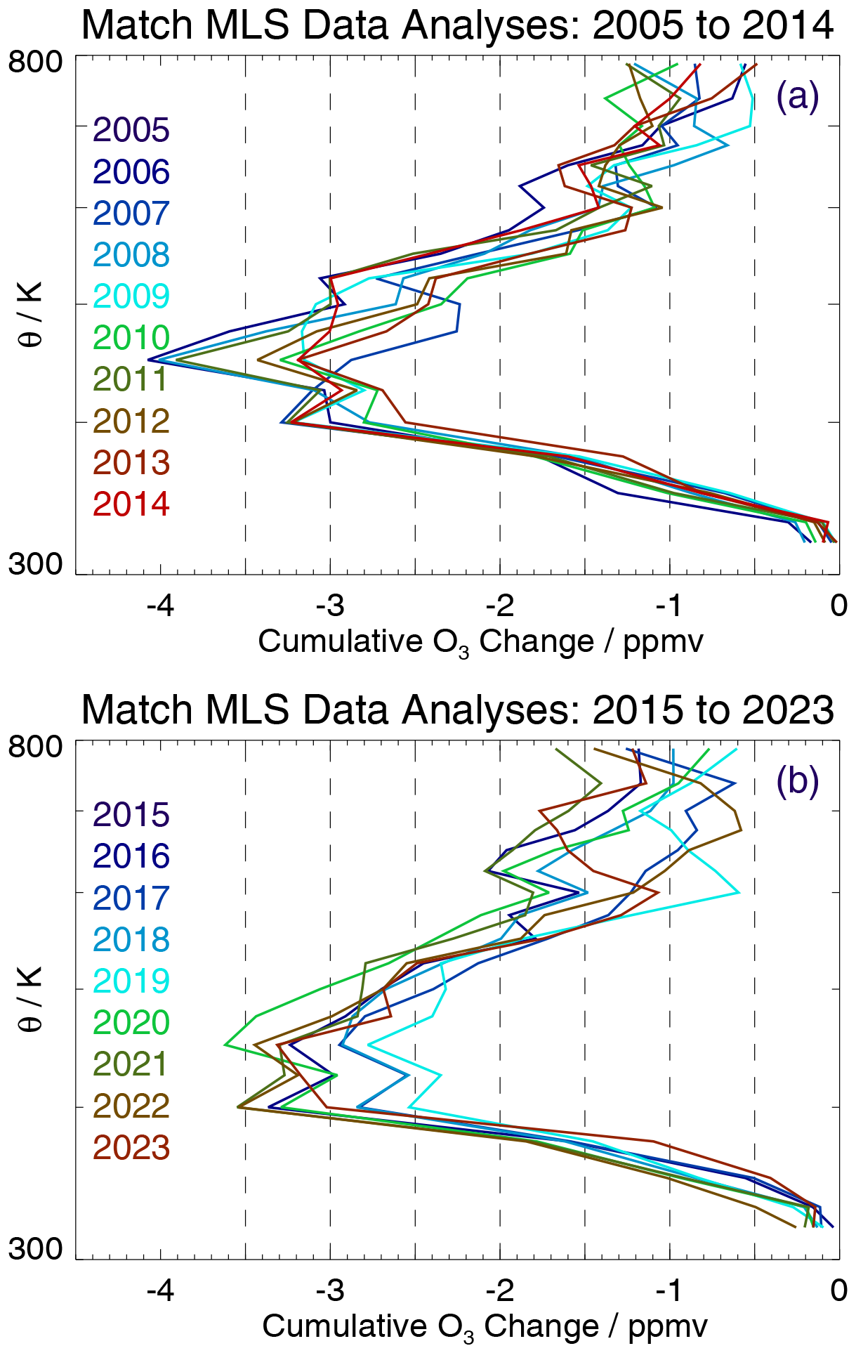
Figure 18 Profiles of maximum cumulative ozone change (with a negative value representing a loss) from the Match technique inside the Antarctic vortex, based on weekly averages in the winter/spring for (a) 2005–2014 and (b) 2015–2023.

We then use the ozone loss values for different dates in September and October to calculate weekly average losses, as we did for earlier analyses presented here. A time series example of the inferred chemical losses from 2005 to 2023 for the week centered on 19 September is provided in Fig. S9, along with a simple linear fit to that series; the positive trend indicated by this linear fit implies smaller chemical losses over time. Figure 19 shows that, while these linear fits lead to some positive trends in the lower part of the Antarctic vortex, there are also oscillations in the loss profiles, and only a few trends are significantly different from zero; we only show the error bars when the trends are deemed to be significant (i.e., further away from zero than the 2σ error values). We also show the trends obtained from fits to the maximum ozone losses from every year between 2005 and 2023; none of these trends are significantly different from zero. Given the small number of Match-derived trends with significant values, we have not pursued any other fits to these chemical ozone loss time series, as we do not expect greater significance from more elaborate MLR fits. The few significant trends obtained from this Match analysis agree, to first order, with the linear trends obtained from our analyses of vortex-average ozone (see the September linear trends in Fig. 12, which are all between 15 and 20 ppbv yr⁻¹). A layer-average of all the September Match trends in chemical ozone loss for potential temperatures below 600 K is slightly less than 10 ppbv yr⁻¹ (not shown), which is somewhat smaller than the September vortex-average trends obtained in the previous section.

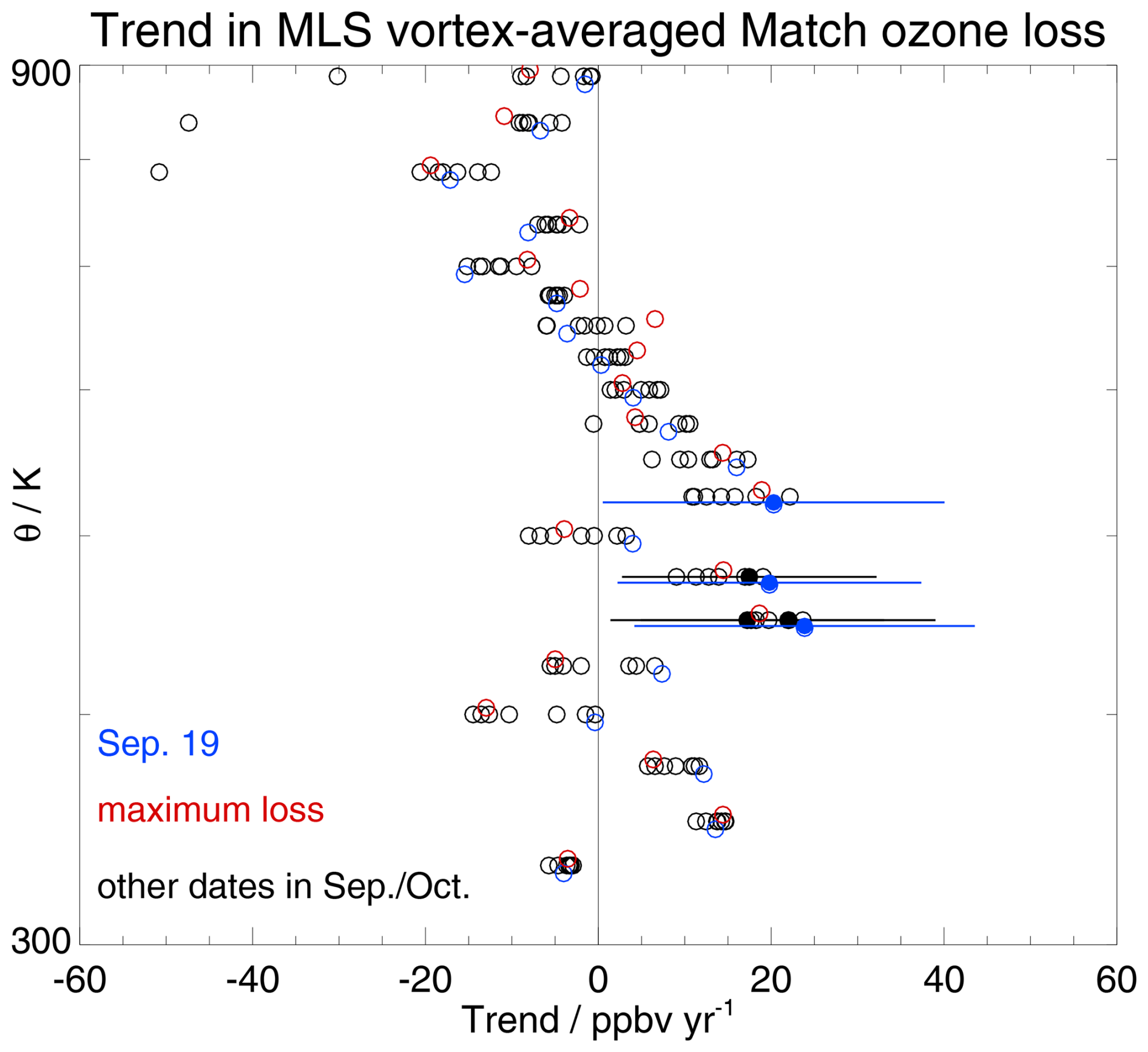
Figure 19 Chemical ozone loss trend profiles inside the Antarctic lower stratospheric vortex from Match-based analyses of MLS data from May through October, for 2005–2023. Only a few trends, marked by the filled circles with associated (2σ) error bars, are significant; for clarity, other error bars are omitted. The blue circles are for the week centered on 19 September, the red circles are trends based on the maximum cumulative losses for each year, and the other points (in black) represent trend values for the other analyzed weeks, from 12 September to 24 October.

4 Discussion and Conclusions

Aura MLS measurements of ozone and other species have played a prominent role in the characterization of global stratospheric change since 2004. Here, we have analyzed the MLS distributions of lower stratospheric Antarctic vortex-average ozone profiles from June to November, along with similarly sampled profiles from two WACCM simulations, driven by MERRA-2 meteorological fields with realistic dynamical and temperature information. One of these simulations uses a scheme with surface ODSs fixed at 1998 values. These chemistry-climate model simulations include effects from downward transport within the vortex, temperature changes and related changes in PSC activity and heterogeneous chemistry, solar flux and EPP variations, and slow changes in greenhouse gas abundances. Wang et al. (2025) have pointed out that Antarctic ozone changes arising from reductions in ODSs should dominate the impacts from greenhouse gases, for now.

The interannual variability in MLS-derived weekly averaged ozone abundances inside the Antarctic vortex is generally well matched by WACCM, although the magnitude of the winter-to-spring ozone decrease is typically slightly smaller in the model. Analyses of probability density functions of ozone profile distributions inside the lower stratospheric Antarctic vortex from 2004 to 2023 reveal shifts as a function of year; in particular, there are some relative decreases in the bins with the smallest ozone abundances. The standard WACCM simulation shows similar shifts and good overall agreement with MLS in lower stratospheric vortex-average ozone linear trends from July to November. Such shifts are qualitatively consistent with past findings of changes in ozone loss saturation over Antarctica (Kuttippurath et al., 2018), based mainly on sonde profile data (and partly on MLS data). The fixed-EESC simulation from WACCM shows no significant trends in lower stratospheric ozone and HCl, as one might expect. We also include MLS and WACCM Antarctic vortex profile comparisons for HNO₃; these show good agreement and no significant trends, except for a negative trend in June–July that requires further investigation.

As has been commented on previously (WMO, 2022), differences in the various approaches used to quantify Antarctic ozone trends make comparisons of trend estimates from different studies problematic. We note that recent Antarctic vortex analyses by Chang et al. (2025) lead to lower stratospheric vortex-average trends of 10 ppbv yr⁻¹ in mid-to-late September and 7 ppbv yr⁻¹ in early October, based on MLS ozone data from 2005 to 2022; this is in good accord with our analyses from 2005 to 2023, both in absolute value and in the sense that October shows smaller trends than September, as has been shown previously (WMO, 2022). Other recent Antarctic trend results (see Sect. 3.2.1) show broad agreement with the positive September trends obtained here for pressures larger than 50 hPa; however, more detailed investigations into some of the larger differences are beyond the scope of this work.

We also used multivariate linear regression fits to weekly mean lower stratospheric vortex-average ozone profiles from MLS and the two WACCM simulations to calculate trends during September and October, when the fastest chemical destruction of ozone occurs. It is useful to analyze both the absolute ozone abundances and the seasonal changes (from early July) in our trend analyses, since both diagnostics should ultimately show robust signs of recovery from the effect of diminishing ODSs. A metric relating to the volume of the sunlit vortex with temperatures low enough to enable NAT PSC formation explains a large part of the year-to-year variability in MLS vortex-average ozone observations. Other proxies used in the regression include two sets of cosine and sine functions with periods of 2.5 and 11 years to represent effects from the quasi-biennial oscillation and longer-term variations, such as the solar cycle (possibly in relation to particle precipitation) or the Antarctic Oscillation; these proxies showed smaller individual impacts on the fits. Reducing the long-term periodicity to 9 or 10 years does not change the trend results appreciably. Regardless of the exact causal links between geophysical variability and Antarctic vortex ozone, we show that applying MLR analyses rather than simple linear regression decreases lower stratospheric Antarctic ozone trend errors by as much as 40 %, while also, as expected, improving the regression fit diagnostics.

Overall, our results indicate that lower stratospheric Antarctic ozone values and seasonal changes through mid-September to mid-October are consistent with a recovery from the impact of ODSs, with significant positive trends between 5 and 16 ppbv yr⁻¹ at 56 to 100 hPa; trend uncertainties (2σ) range from ∼ 8 ppbv yr⁻¹ at 68–56 hPa to ∼ 4 ppbv yr⁻¹ at 100 hPa. The WACCM results agree well with those from MLS. As expected, the model simulation with fixed ODSs leads to Antarctic ozone trends in the lower stratosphere that are consistent with zero trend. We estimate that the positive ozone trends we obtain for mid-September correspond to an average partial lower stratospheric (pressures larger than 46 hPa) column change of 1 to 1.5 DU yr⁻¹. These values are within the range of Antarctic total column ozone change (∼ 25–30 DU between 2000 and 2025, or ∼ 1–1.2 DU yr⁻¹) obtained from various models (e.g., Dhomse et al., 2018; Amos et al., 2020). However, partial column ozone changes of this magnitude are still less than half of the amount needed for ozone to return to pre-ozone-hole values over Antarctica, which models predict will occur shortly after mid-century (WMO, 2022).

Finally, we explored trends in chemical ozone loss as quantified by the Match technique, whereby MLS measurements of ozone are tracked along trajectories to estimate vortex-average chemical ozone loss during winter/spring. While the Match results show some reductions in seasonal lower stratospheric Antarctic chemical ozone loss over the 2005 to 2023 period, consistent with a positive trend (based on simple linear regression) of order 5–15 ppbv yr⁻¹, we obtain statistical significance (as defined in this work) for only a limited subset of cases in mid-to-late September. However, many of the lower stratospheric Match results are consistent with a zero trend; there is also a large spread in these trend results as a function of height (potential temperature) inside the vortex. We do not expect that use of a more sophisticated regression fit would produce much improvement in the significance of trends in chemical ozone loss, given the values of the linear-only regression trends and their error bars.

These analyses represent new facets of the characterization of the recovery of Antarctic vortex ozone as ODSs diminish, which has been a key goal of the Aura mission. Our results support the robust detection of significant recovery in lower stratospheric Antarctic ozone during parts of September and October over the 2005–2023 period, at pressures larger than 50 hPa. This work adds to the body of evidence underscoring the importance of the 1987 Montreal Protocol and its Amendments, as this international agreement has been a shining example of how policymakers around the world can come together to solve a global environmental problem. However, the upcoming dearth of daily global height-resolved stratospheric composition measurements after the end of the Aura mission (Salawitch et al., 2025) will greatly hinder the ability to detect and understand short- and longer-term changes in stratospheric composition and their effects on the Antarctic ozone hole.