the Creative Commons Attribution 4.0 License.
the Creative Commons Attribution 4.0 License.
 | 15 Jan 2024
Exploring the ENSO modulation of the QBO periods with GISS E2.2 models
Kevin J. DallaSanta
Clara Orbe
David H. Rind
Jeffrey A. Jonas
Larissa Nazarenko
Gavin A. Schmidt
Gary Russell
Observational studies have shown that the El Niño–Southern Oscillation (ENSO) exerts an influence on the Quasi-Biennial Oscillation (QBO). The downward propagation of the QBO tends to speed up and slow down during El Niño and La Niña, respectively. Recent results from general circulation models have indicated that the ENSO modulation of the QBO requires a relatively high horizontal resolution, and that it does not show up in the climate models with parameterized but temporally constant gravity wave sources. Here, we demonstrate that the NASA Goddard Institute for Space Studies (GISS) E2.2 models can capture the observed ENSO modulation of the QBO period with a horizontal resolution of 2∘ latitude by 2.5∘ longitude but with its gravity wave sources being parameterized interactively. This is because El Niño events lead to more vigorous gravity wave sources generating more absolute momentum fluxes over the equatorial belt, as well as less filtering of these waves into the tropical lower stratosphere through a weakening of the Walker circulation. Various components of the ENSO system, such as the sea surface temperatures, the convective activities, and the Walker circulation, are intimately involved in the generation and propagation of parameterized gravity waves, through which ENSO modulates the QBO period in GISS E2.2 models.
- Article
(8598 KB) - Full-text XML
-
Supplement
(1736 KB) - BibTeX
- EndNote


The Quasi-Biennial Oscillation (QBO) dominates the interannual variability in the tropical stratosphere (Baldwin et al., 2001), whereas the El Niño–Southern Oscillation (ENSO) is the primary mode of interseasonal–interannual variability over the tropical Pacific Ocean (Wang et al., 2017). It is well known that both the QBO and the ENSO have far-reaching implications for global weather and climate systems (Hamilton et al., 2015; Philander, 1990; Sarachik and Cane, 2010; Domeisen et al., 2019).
The QBO and the ENSO defy linear relationships (Angell, 1986; Xu, 1992; Hu et al., 2012) as highlighted by that fact that while the QBO and ENSO indices are negatively correlated before the 1980s and positively correlated after the 1980s (Garfinkel and Hartmann, 2007; Domeisen et al., 2019; Rao et al., 2020c), they are virtually uncorrelated over the longer periods from 1953 to recent times (Garfinkel and Hartmann, 2007; Geller et al., 2016b, see their Fig. 5 for details). However, Maruyama and Tsuneoka (1988) spotted an intriguing connection between the anomalously short easterly phase of the QBO at 50 hPa in 1987 and the El Niño event that persisted throughout that year. Based on the results from a mechanistic model, Geller et. al. (1997) suggested that the equatorial sea surface temperatures (SSTs) modulate the wave momentum fluxes into the stratosphere and thus the QBO. Remarkably, an observational study conducted by Taguchi (2010) demonstrated that the downward propagation of the QBO tends to speed up during El Niño and slow down during La Niña, whereas the amplitude of the QBO tends to be smaller during El Niño and larger during La Niña, respectively. Using radiosonde data from 10 near-equatorial stations distributed along the Equator, Yuan et al. (2014) found that the ENSO modulation of the QBO period is more robust than that of the QBO amplitude, which is likely due to the fact that the QBO periods are characterized by a high degree of zonal uniformity, whereas the QBO amplitudes exhibit zonal asymmetries of about 10 % (Hamilton et al., 2004, see their Fig. 15).
The QBO influences the distribution and transport of various chemical constituents (Zawodny and McCormick, 1991; Trepte and Hitchman, 1992; Hasebe, 1994; Kawatani et al., 2014): the extratropical circulation in the winter stratosphere (Holton and Tan, 1980; Labitzke, 1982; Rao et al., 2020a, b, 2021), tropical moist convection (Collimore et al., 2003; Liess and Geller, 2012), the activities of tropical cyclones (Gray, 1984; Ho et al., 2009), the ENSO (Gray et al., 1992; Huang et al., 2012; Hansen et al., 2016), the Hadley circulation (Hitchman and Huesmann, 2009), the tropospheric subtropical jet (Garfinkel and Hartmann, 2011a, b; Kumar et al., 2022), the boreal summer monsoon (Giorgetta et al., 1999; Yoden et al., 2023), and the Madden–Julian Oscillation (Yoo and Son, 2016). Thus, it is imperative that weather and climate models have the capacity to simulate the ENSO modulation of the QBO.
Various studies have investigated how the ENSO exerts its influence over the QBO in climate models. Schirber (2015) conducted two sets of experiments to explore this issue using the general circulation model European Centre/Hamburg 6 (ECHAM6) wherein a convection-based gravity wave (GW) scheme was newly implemented. The first set of experiments was called QBOW where the initial QBO configurations consisted of a westerly jet above the 10 hPa level and an easterly jet below that level. Likewise, in the second set of experiments named as QBOE, the initial QBO conditions included an easterly and westerly jet above and below the 10 hPa level, respectively. Schirber showed that for QBOW, the ensemble mean period of the QBO from the El Niño runs is shorter than that from the La Niña runs, whereas for QBOE the ensemble mean periods are comparable between the El Niño and the La Niña runs. Schirber also noted that there is no systematic change in amplitude of the QBO jets between the El Niño and La Niña runs. Using version 3 of the EC-Earth Consortium's climate model with a triangular spectral truncation at total wavenumber 255 (T255, horizontal resolution of ∼ 0.54∘), Christiansen et al. (2016) reported that each of 10 ensemble members simulated a faster QBO descent rate during El Niño than during La Niña, and that their ensemble mean QBO phase speeds were comparable to those derived from the reanalyses.
Employing two atmospheric general circulation models (AGCM) developed under the Model for Interdisciplinary Research on Climate (MIROC) framework, Kawatani et al. (2019) investigated the possible mechanism of the ENSO modulation of the QBO. They first compared a 100-year perpetual El Niño run with a 100-year perpetual La Niña run from the MIROC-AGCM with T106 horizontal resolution and 500 m vertical spacing in the stratosphere without any nonorographic GW parameterizations. Then they repeated the two AMIP-style perpetual El Niño and La Niña experiments but using the atmospheric part of the Model for Interdisciplinary Research on Climate, Earth System Model (MIROC-ESM) with T42 horizontal resolution and 700 m vertical spacing in the stratosphere where the effects of nonorographic GWs are parameterized and the GW sources are held constant in time. They found that the MIROC-AGCM simulates shorter QBO periods during El Niño than during La Niña because of the larger equatorial vertical wave fluxes of zonal momentum in the uppermost troposphere and consequently the much larger resolved GW forcing in the stratosphere during warm ENSO phase. However, they found almost no difference in the average QBO periods simulated by the MIROC-ESM between El Niño and La Niña because the QBO was generated by the parameterized nonorographic GW forcing in the model where the GW sources were held constant in time and thus did not respond to the SST changes associated with the ENSO cycle. (See their Figs. 16 and 18 for more details.)
Using more than a dozen models from five modeling centers with their horizontal resolutions ranging from T42 (∼ 2.79∘) to T1279 (∼ 0.14∘), Serva et al. (2020) found that a relatively high horizontal resolution above T159 (∼ 0.75∘) was desirable to simulate the observed modulation of the QBO descent rate under strong ENSO events, whereas the amplitude response is generally weak at any horizontal resolution. They also pointed out that over-dependence on parameterizing the effects of GWs with temporally invariant sources is detrimental to the realistic simulation of the coupling between the ocean and the tropical stratosphere in current climate models.
As far as the ENSO modulation of the QBO period is concerned, both Kawatani et al. (2019) and Serva et al. (2020) emphasized the importance of a relatively high horizontal resolution and the inadequacy of noninteractive GW sources. However, the exploratory work of Schirber (2015) shows that the ENSO modulation of the QBO period can, to some extent, be simulated in the GCM ECHAM6 with T63 and an associated Gaussian grid of ∼ 1.9∘ horizontal resolution, because rather than being held constant in time, the properties of noninteractive GW sources in the tropics are determined by the simulated convection which is modulated by ENSO phases.
Rind et al. (1988) pioneered the use of meteorologically interactive GW sources in the Goddard Institute for Space Studies (GISS) climate models. These sources included flow over topography, convection, wind shear, and, in Rind et al. (2007), wind deformation. By increasing the vertical resolution and revising the formulations, various versions of the GISS models subsequently simulate a spontaneous QBO (Rind et al., 2014, 2020; DallaSanta et al., 2021). The GISS E2.2 models are comprehensive climate models optimized for the middle atmosphere (Rind et al., 2020; Orbe et al., 2020). Their outputs have been submitted to the archive of the Coupled Model Intercomparison Project Phase 6 (CMIP6). Bushell et al. (2022) pointed out that most of the current climate models are highly dependent on parameterized nonorographic GW forcing to simulate a QBO. Unsurprisingly, DallaSanta et al. (2021) found that the parameterized convective GWs play a dominant role in generating the spontaneous QBO in the GISS E2.2 models.
High-resolution AGCMs can realistically simulate atmospheric structure without resorting to parameterized GWs (e.g., Watanabe et al., 2008), but the associated computational cost is too high for the earth system modeling at the present time. Thus, most climate models still require GW parameterization schemes. What is more, Fig. 4c in Serva et al. (2020) shows that two different GW parameterization schemes employed by the same T255 model make a drastic difference in the ENSO modulation of the QBO period. Specifically, one scheme makes a difference of about 10 months in the ensemble mean QBO period between El Niño and La Niña episodes while the other hardly makes an appreciable difference. In other words, improperly parameterized GW forcing could destructively interfere with the ENSO modulation of the QBO period in high-resolution climate models. Therefore, it is imperative that GW forcing be parameterized properly in climate models with a variety of horizontal resolutions.
In this paper, we will evaluate the ENSO modulation of the QBO simulated by the GISS E2.2 models against the observed modulation and explore how the ENSO modulates the QBO period in those models. Section 2 describes the observations and GISS E2.2 models used in this study and outlines our methods of analyses. Section 3 revisits the ENSO modulation of the QBO from the observational point of view. Section 4 evaluates the ENSO modulation of the QBO period in the historical runs simulated by four versions of the GISS E2.2 models. Section 5 explores the physical mechanisms underlying the simulated modulation. Conclusions and discussion are presented in Sect. 6.
2.1 Observations
To study the observed QBO, we use the monthly mean zonal winds provided by Free University of Berlin (FUB). The FUB data were produced by combining the radiosonde observations at the following three equatorial stations: Canton Island near 172∘ W, 3∘ S (closed in 1967), Gan/Maldive Islands near 73∘ E, 1∘ S (closed in 1975), and Singapore near 104∘ E, 1∘ N (Naujokat, 1986). We use 63 years (i.e., 756 months) of the FUB data ranging from 1953 to 2015 at the following seven pressure levels: 70, 50, 40, 30, 20, 15, and 10 hPa.
The observed ENSO index is derived from the National Oceanic and Atmospheric Administration (NOAA) Extended Reconstructed SST (ERSST) v5 datasets (Huang et al., 2017a) provided by National Centers for Environmental Information (NCEI). ERSST produced on a 2∘ × 2∘ grid is derived from the International Comprehensive Ocean–Atmosphere Data Set (ICOADS). The latest version of ERSST, version 5, uses new datasets from ICOADS release 3.0 SST, combining information from Argo floats above 5 m and Hadley Centre Ice-SST version 2 ice concentrations.
The monthly outgoing longwave radiation (OLR) on a 2.5∘ × 2.5∘ grid from NCEI (Liebmann and Smith, 1996) is used as a proxy for tropical convection since cloud top temperatures are negatively correlated with cloud height in the tropics (Salby, 2012). The ERA5 (Hersbach et al., 2020) monthly mean zonal winds were employed to depict the observed Walker circulation against which we evaluate those simulated by GISS E2.2 models. The employed OLR and zonal winds range from 1979 to 2015.
2.2 Description of the models and simulations
GISS E2.2 is a climate model specially optimized for the middle atmosphere (Rind et al., 2020; Orbe et al., 2020) and its output was submitted to the Coupled Model Intercomparison Project Phase 6 (CMIP6) archive. The horizontal resolution of all GISS E2.2 models is 2∘ (latitude) by 2.5∘ (longitude) for the atmosphere and the model extends from the surface to 0.002 hPa (∼ 89 km) with 102 vertical layers. (For more details, see Table 1 in Rind et al., 2020.) Note that an adequate vertical resolution is necessary for climate models to internally generate a spontaneous QBO (Scaife et al., 2000; Richter et al., 2014; Rind et al., 2014, 2020; Geller et al., 2016a; Butchart et al., 2018).
With respect to atmospheric chemistry, the atmospheric component of the GISS E2.2 models was configured in two ways for CMIP6. The first configuration is denoted as NonINTeractive (NINT) where the fields of radiatively active components, such as ozone and multiple aerosol species, are specified from previously calculated offline fields (Kelley et al., 2020; Miller et al., 2021). The second configuration includes interactive gas-phase chemistry and a mass-based (one-moment aerosol (OMA)) aerosol module, where aerosols and ozone are driven by emissions and calculated prognostically (Bauer et al., 2020; Nazarenko et al., 2022). The above-mentioned NINT and OMA configurations correspond to physics-version = 1 (“p1”) and physics-version = 3 (“p3”), respectively, in the CMIP6 archive.
The basic dynamics and tropospheric physics structure of the GISS E2.2 models were based on the GISS E2.1 model (Kelley et al., 2020). One version of the cloud parameterization schemes used in E2.2, termed as “standard physics” (SP), has not been fully upgraded to the state-of-the-art module customized for E2.1 which has only 40 vertical layers up to 0.1 hPa (Rind et al., 2020). Accordingly, E2.2–SP has a younger sibling, E2.2–AP, whose cloud parameterization schemes, termed as “altered physics” (AP), are more aligned with those in E2.1 and whose outputs were thus favored for the submission to the CMIP6 archive. “Altered physics” in E2.2–AP brings about a somewhat different response to SST as compared with the “standard physics” in E2.2–SP.
The QBO in the GISS models are mainly driven by GWs (DallaSanta et al., 2021). The phase velocities and momentum fluxes of GW sources are coupled to convective cloud-top-pressure altitudes, convective mass fluxes, background wind fields, and so on (Rind et al., 1988, 2014, 2020). Specifically, intrinsic phase velocities ±10 and ±20 m s−1 of GWs generated by convection are Doppler-shifted by local background winds for shallow convection and for convection penetrating above the altitudes of the 400 hPa pressure level, respectively. Convective gravity wave momentum flux magnitude is determined by the density and Brunt–Vaisala frequency at the top of convective region and the vertically integrated mass flux over the convective region. The mass flux in the model is strongly related to the depth of penetration, and thus this parameterization is somewhat similar to that of the other models that use convective sources. (See Eq. 7 in Rind et al., 1988, and the further discussion in Rind et al., 2014.)
Using the same GW parameterization scheme, both E2.2–SP and E2.2–AP are included in this study to gain insight into the mechanisms through which ENSO modulates the QBO period despite the fact that the outputs of E2.2–SP were not submitted to the CMIP6 archive.
Table 1The model configurations and respective ensemble simulations. Note: n/a – not applicable.
∗ E2-2-G.amip.r[1–5]i1p3f1 in the CMIP6 archive are the outputs of the same model but range from 1979 to 2014.
We will look into two atmosphere-only (AMIP) ensemble simulations where the evolution of SST and sea ice fraction (SIF) is specified and two coupled ensembles where the respective model atmosphere interacts with the ocean component termed as the GISS Ocean v1 (GO1), which extends from the surface to the ocean floor with 40 vertical layers and has a horizontal resolution of 1∘ latitude by 1.25∘ longitude (Schmidt, et al., 2014; Kelley et al., 2020). Table 1 lists the four model configurations and their respective ensemble simulations investigated in this study.
The first two ensembles in Table 1 were generated by AMIP–OMA–SP and AMIP–OMA–AP models where the SST and SIF from the HadISST1 dataset (Rayner et al., 2003) were prescribed for the simulations between 1870 and 2014, whereas their climatological annual cycles over the 1876–1885 period were specified for the earlier simulations between 1850 and 1869. Both AMIP–OMA–SP and AMIP–OMA–AP prognostically calculate the concentrations of ozone, methane, chlorofluorocarbons, aerosols, and so on. The main differences between AMIP–OMA–SP and AMIP–OMA–AP reside in the package of cloud parameterization schemes, which leads to their different responses to SST and thus may have important implications for simulating the ENSO modulation of the QBO period. We discarded the simulations ranging from 1850 to 1869 in this study because they are irrelevant to the ENSO modulation of the QBO in the absence of interannual variations in the prescribed SST over that period. Note that the two extended historical AMIP simulations from 1870 to 2014 listed in Table 1 were not submitted to the CMIP6 archive. However, AMIP–OMA–AP did generate a five-member ensemble over the 1979–2014 period that was submitted to the CMIP6 archive and tagged as E2-2-G.amip.r[1–5]i1p3f1. It is worth noting that the climatological characteristics over the 1979–2014 period derived from the AMIP–OMA–AP ensemble listed in Table 1 are comparable to those derived from E2-2-G.amip.r[1–5]i1p3f1, albeit the climate trajectories of the individual ensemble members over the 1979–2014 period are expected to differ between those two ensembles starting from January 1850 and January 1979, respectively, due to the chaotic nature of climate systems.
The other two ensembles in Table 1 were generated by the Coupled–NINT–SP and Coupled–NINT–AP where the respective atmospheric components are coupled with GO1. Both the Coupled–NINT–SP and Coupled–NINT–AP simulations were performed with the prescribed atmospheric composition generated from the AMIP-style OMA simulations using the historical forcings over the 1850–2014 period. As mentioned earlier with regard to the AMIP–OMA–SP and AMIP–OMA–AP runs, the difference in cloud physics between the Coupled–NINT–SP and Coupled–NINT–AP models is exploited to gain a deeper insight into the mechanisms through which the ENSO modulates the QBO periods. Both Coupled–NINT–SP and Coupled–NINT–AP ensemble runs started from January 1850 and ended in December 2014.
Since there are no interannual variations in the prescribed SST over the 1850–1869 period for both the AMIP–OMA–SP and AMIP–OMA–AP runs, our analyses focus on the 1870–2014 period for those two ensembles. For the sake of conciseness and consistency, we also discarded the outputs from two coupled runs over the 1850–1869 period. In short, we only use the data over the 1870–2014 period from the ensemble simulations listed in Table 1.
2.3 Methods
2.3.1 Data processing
We first fill the missing FUB zonal winds at the 10 hPa level for the first 3 years by linear extrapolation in log-pressure height. Then, we remove the climatological mean zonal winds from the resultant monthly zonal winds to obtain the monthly anomalies of zonal winds. These anomalous monthly zonal winds will be used for our observational study in this paper.
To obtain the ENSO index from the ERSSTv5 data ranging from 1953 to 2015, we use the same method to calculate the Oceanic Niño Index (ONI) as the Climate Prediction Center (CPC) of NOAA. Namely, the ONI is defined as a 3-month running mean of ERSSTv5 SST anomalies in the Niño 3.4 region (5∘ S–5∘ N, 120–170∘ W) based on centered 30-year base periods updated every 5 years (see https://origin.cpc.ncep.noaa.gov/products/analysis_monitoring/ensostuff/ONI_v5.php, last access: 6 November 2023). This method ensures a proper identification of El Niño and La Niña by taking the secular changes in SSTs into account. The SST anomalies (SSTA) are defined as the deviations of the SST from its climatological annual cycle over a selected base period. Specifically, the SSTA during 1951–1955 are based on the 1936–1965 base period, the SSTA during 1956–1960 are based on the 1941–1970 base period, and so on. Thus, as the CPC of NOAA we used the ERSSTv5 SST from January 1936 to January 2016 period to obtain the ONI from January 1953 to December 2015.
Following the CPC of NOAA, we refer to El Niño or La Niña episodes as the periods when the ONIs are greater than +0.5 ∘C or less than −0.5 ∘C for at least 5 consecutive months, respectively. Since the temperature measurement is only accurate to the tenths place, all our calculated ONIs are rounded to the nearest tenth. Based on the rounded ONIs, our identified El Niño and La Niña episodes are almost identical to those listed at the above-mentioned website of NOAA CPC. Accordingly, we identified 21 El Niño and 15 La Niña events between 1953 and 2015.
Similarly, when we explore how GISS E2.2 models simulate the ENSO modulation of the QBO we define the ONI as a 3-month running mean of prescribed SSTA from the AMIP–OMA–SP and AMIP–OMA–AP runs, or simulated SSTA from the Coupled–NINT–SP and Coupled–NINT–AP runs in the Niño 3.4 region (5∘ S–5∘ N, 120–170∘ W) based on centered 30-year base periods updated every 5 years. Here, the SSTA are also defined as the deviations of the SST from its climatological annual cycle over a selected base period. Specifically, the SSTA during 1886–1890 are based on the 1871–1900 base period, the SSTA during 1891–1895 are based on the 1876–1905 base period, the SSTA during 1991–1995 are based on the 1976–2005 base period, and the SSTA during 1996–2000 are based on the 1981–2010 base period. In addition, the SSTA during the earliest 1870–1885 and latest 2011–2014 spans are ad hoc based on the 1870–1899 and 1985–2014 base periods, respectively. Thus, we used the specified or simulated SSTs over the 1870–2014 period to obtain the ONI from February 1870 to November 2014.
For the sake of consistency, we also apply this same filtering procedure to all other fields simulated by GISS E2.2 models such as OLR, zonal winds, resolved wave forcing, parameterized GW forcing, absolute convective momentum flux, and so on. Thus, the simulated zonal winds and other quantities were subjected to a 3-month moving averaging. In addition, the secular trends of zonal winds and those other quantities were also removed due to the adoption of the consecutive 5-year base periods. To further simplify our analyses, all processed model outputs used in this study range from 1871 to 2013. In other words, we also discarded the processed model outputs over the period between February 1870 and December 1870 and that between January 2014 and November 2014.
Employing the above-mentioned criteria that were used to identify the observed ENSO events between 1953 and 2015, we identified 34 El Niño and 30 La Niña events over the period from 1871 to 2013 from the specified HadISST1 dataset. We further found that the five members of the Coupled–NINT–SP ensemble simulations generated 31, 31, 29, 35, and 36 El Niño events and produced 34, 34, 35, 37, and 35 La Niña events, respectively, over the period from 1871 to 2013. In parallel, we identified 37, 42, 40, 37, and 38 El Niño events and 38, 43, 37, 40, and 39 La Niña events from the SSTs simulated by the five members of the Coupled–NINT–AP ensemble, respectively, over the same period.
2.3.2 Statistical analysis
Following Wallace et al. (1993), we decomposed both the observed and simulated equatorial zonal winds between 10 and 70 hPa pressure levels into two leading pairs of empirical orthogonal functions (EOFs) and principal components (PCs) because they typically account for more than 90 % of the vertical structure variance (Wallace et al., 1993; DallaSanta et al., 2021). For the sake of robustness, we excluded the FUB data after 2015 because the first two EOFs explain no more than 60 % of total variance during the 2016 and 2019/2020 QBO disruptions (Anstey et al., 2021). As a result, the QBO variability can be, to a very good approximation, compactly depicted by the trajectory of (PC1(t),PC2(t)) in a linear space spanned by the first two orthonormal EOFs.
As in previous studies (Wallace et al., 1993; Taguchi, 2010; Christiansen et al., 2016; Serva et al., 2020; DallaSanta et al., 2021), the instantaneous amplitude (am) and phase (ψ) of the QBO are defined as
Differentiating Eq. (2) with respect to time yields the instantaneous phase speed of the QBO:
Using Eqs. (1)–(3) and the monthly processed FUB data from 1953 to 2008, Taguchi (2010) obtained 672 months of am and ψ′ and partitioned each time series of {am} and {ψ′} into 16 categories. The 16 categories correspond to the 16 combinations of four QBO phase quadrants at the 50 hPa level and four seasons. Using a bootstrap (Chernick, 2007) method, Taguchi (2010) seminally illuminated the annual synchronization of the QBO. Taguchi (2010) further used the bootstrap method to show that the QBO signals during El Niño episodes exhibit weaker amplitude in 6 out of 16 categories and faster phase propagation in 8 out of 16 categories at a 90 % or 95 % confidence level (refer to Fig. 6 in Taguchi, 2010).
It is worth pointing out that while Taguchi's conclusion is physically meaningful, his statistical analysis is not robust concerning the ENSO influence on the QBO. For instance, there are 18 sample points in the (MAM, E) category where MAM stands for the months of boreal spring, i.e., March, April, and May, while E indicates that the QBO winds at the 50 hPa level are easterly. As Taguchi (2010) mentioned, the actual (i.e., effective) sample size should be 6 rather than 18, due to the data clustering. Among those 18 months of data, there are 6 months for El Niño conditions and 1 month for La Niña conditions. Also pointed out by Taguchi (2010), actual sample sizes are two and one for El Niño and La Niña conditions, respectively, in the (MAM, E) category. It is hard to imagine that we can infer any meaningful result from one La Niña sample point and two El Niño sample points out of the sample with its size being six, because Chernick (2007) points out that sample sizes less than 10 are too small for sample estimates to be reliable, even in “nice” parametric cases, and that such sample sizes are, as expected, also too small for bootstrap estimates to be of much use (see Chernick, 2007, p. 174). With regard to the above-mentioned (MAM, E) category, the following conclusion is evidently not robust: the QBO amplitude during El Niño episodes is weaker than that during La Niña episodes at a 95 % confidence level (refer to Fig. 6b in Taguchi, 2010), because one extreme La Niña sample point and/or a couple of extreme El Niño sample points can influence the outcome of the statistical test.
Since we have observed 21 El Niño and 15 La Niña events between 1953 and 2015, the sample sizes of El Niño and La Niña appear large enough for us to conduct a classical parametric test. Namely, we have two samples: one consists of 21 independent El Niño events and the other contains 15 independent La Niña events. For each ENSO event, we define the amplitude [am] and phase speed [ψ′] of the QBO as the monthly am in Eq. (1) and the monthly ψ′ in Eq. (3) that are averaged over the number of months of that event. Thus, both the El Niño sample and the La Niña sample are described by two statistics [am] and [ψ′], namely, the mean amplitude and mean phase speed of the QBO for an ENSO event. (Note that in this paper, a quantity enclosed by a pair of square brackets denotes the average value of that quantity over the duration (i.e., the total number of months) of an ENSO event.)
We employ Welch's t test (Moser and Stevens, 1992) to infer whether there is a significant difference in [am] or [ψ′] between the El Niño and La Niña population means. For the sake of conciseness, we will refer to [am] and [ψ′] as A and Ψ′, respectively, in this subsection and Sect. 3. (In other words, we will no longer use the mnemonic notations [am] and [ψ′] in this subsection and Sect. 3 wherein we will instead employ A and Ψ′, respectively, for brevity.)
To examine whether the sample mean QBO amplitude is significantly different between El Niño and La Niña, we first construct the statistic,
where and are the values of As that are averaged over the number of the El Niño and La Niña events, respectively, with the standard error of their difference being
where and are the corrected sample standard deviation of A for El Niño and La Niña, respectively, while N1 and N2 are the sample sizes of El Niño and La Niña events. According to Moser and Stevens (1992), the degrees of freedom for the t distribution is
2.3.3 Analysis of the QBO forcings
The QBO owes its existence to wave-mean flow interaction (Lindzen and Holton, 1968; Holton and Lindzen, 1972; Plumb, 1977). The evolution of zonal mean zonal winds is governed by the transformed Eulerian mean (TEM) momentum equation formulated in pressure coordinates on a sphere (Andrews et al., 1983):
where the Eliassen–Palm flux F is defined as
and its divergence as
In Eq. (7), t denotes time, p pressure, φ latitude, (uvω) “velocity” in (longitude, latitude, pressure) coordinates, a the mean radius of earth, ρ0 pressure-dependent basic density, and f the Coriolis parameter. In Eq. (8), ε is defined as
where θ denotes potential temperature, T temperature, and κ the ratio of the gas constant to the specific heat at constant pressure. Note that in Eqs. (7)–(10) primes denote departures from the zonal means which are represented by overbars, and residual meridional and vertical velocities, i.e., and , are defined as and , respectively.
On the right side of Eq. (7), the first term, , is the forcing from the GWs parameterized in E2.2 models; the second term, , is the forcing driven by the waves resolved by GISS E2.2 models; the third term, , is associated with the TEM advection; and the last term, , is the zonal component of friction or other nonconservative mechanical forcings (Andrews et al., 1987). Since is small as far as the QBO is concerned, we will focus on analyzing the first three terms of Eq. (7) and ignore the last term of that equation in this study.
In the era of big data, bootstrap methods are a powerful tool that is used to analyze uncertainties for any machine learning model. However, the bootstrap methods cannot get something for nothing. They are not reliable if the sample size is too small. In this section, we will use the classical parametric method outlined in Sect. 2.3.2 to revisit the ENSO modulation of the QBO using the FUB data described in Sect. 2.1.
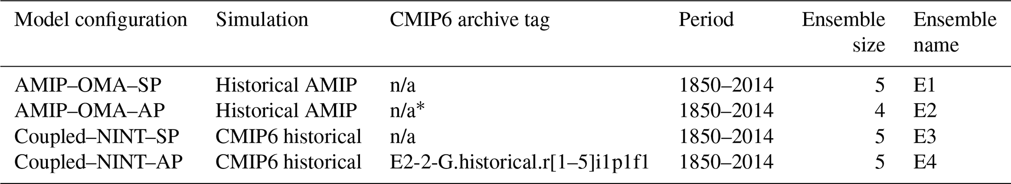
The solid and dashed black lines in Fig. 1 depict the two leading EOFs derived from the monthly anomalies of the FUB zonal winds between 1953 and 2015. The vertical structures of those two EOFs are very similar to those depicted in Fig. 2a of Taguchi (2010) who used the FUB zonal winds from 1953 to 2008. Our calculated two leading EOFs account for 92.6 % of the vertical structure variance (57.1 % by EOF1 and 35.5 % by EOF2) which is slightly smaller than the value of 96.1 % shown in Taguchi (2010). Note that this discrepancy is not mainly due to the difference in the adopted time spans. When we use the monthly anomalies of the FUB zonal winds between 1953 and 2008, the resultant two leading EOFs account for 92.9 % of the vertical structure variance (57.0 % by EOF1 and 35.9 % by EOF2). Coy et al. (2020) pointed out that the descent of the QBO winds varies at intraseasonal, seasonal, and interannual timescales (see their Fig. 1 for more details). Thus, it is natural that two leading EOFs explain more variance in the FUB zonal winds when those winds have been deseasonalized and subjected to a 5-month running averaging.
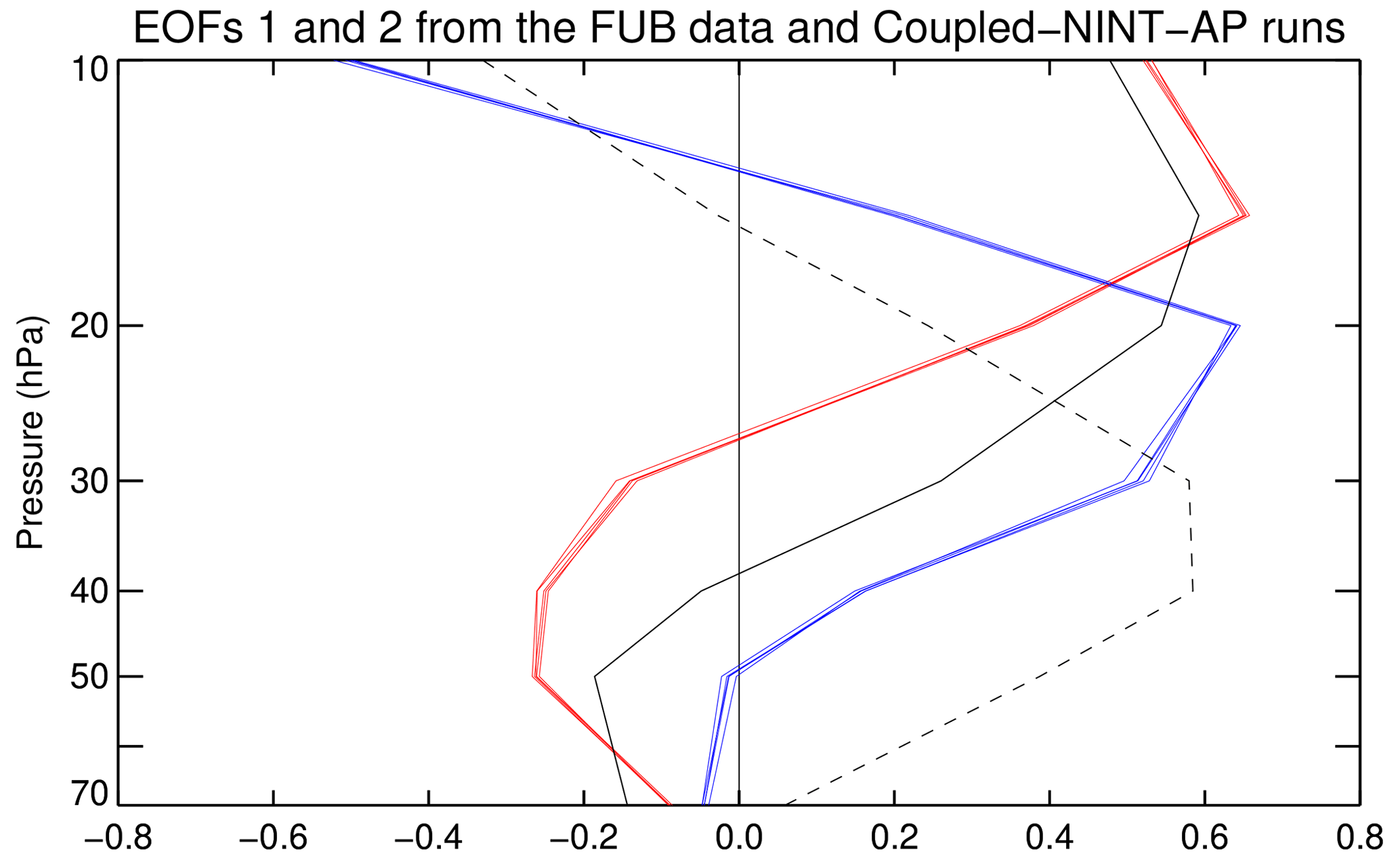
Figure 1Black lines depict the first (solid) and second (dashed) orthonormal eigenvectors derived from the monthly FUB zonal wind anomalies between 1953 and 2015. Colored lines delineate the first (red) and second (blue) orthonormal eigenvectors derived from the deseasonalized and smoothed equatorial zonal mean zonal winds between 1873 and 2013 from the five Coupled–NINT–AP runs.
As mentioned before, there are 21 El Niño and 15 La Niña episodes between 1953 and 2015, i.e., N1=21 and N2=15. Our calculations yield m s−1, m s−1, ν=33, and . Apparently, , which suggests that the QBO amplitude is smaller during El Niño than during La Niña. Performing a two-tailed test, however, we find that the QBO amplitudes during El Niño episodes are not statistically different from those during La Niña episodes at the 5 % significance level. This is consistent with the finding of the observational study by Yuan et al. (2014), namely, the ENSO modulation of the QBO amplitude is less robust than that of the QBO period. This is also consistent with the findings of the modeling studies conducted by Schirber (2015) and Serva et al. (2020).
Note that when we use the FUB zonal winds and the ERSSTv5 data over the 1953–2008 period as did Taguchi (2010), our calculations yield N2=13, m s−1, m s−1, ν=29, and . A two-tailed test shows that the difference in the QBO amplitude between El Niño and La Niña is not statistically significant at the 5 % significance level either.
Apparently, no matter whether we use the FUB data over the 1953–2008 period or over the 1953–2015 period, the influence of the ENSO on the QBO amplitude is not statistically significant at the 5 % significance level. Thus, we will not further explore whether GISS E2.2 models can simulate the ENSO modulation of the QBO amplitude in this study.
To examine whether the sample mean QBO phase speed is significantly different between El Niño and La Niña, we similarly use Eqs. (4)–(6) except that and are replaced by and , respectively. Based on the data from 1953 to 2015, we obtained N1=21 and N2=15, radians per month, radians per month, ν=28, and t=2.36. Evidently, , indicating that the phase speed of the QBO is greater during El Niño than during La Niña. Performing a two-tailed test, we ascertain that the phase speed of QBO during El Niño episodes are statistically different from those during La Niña episodes at the 5 % significance level. Put in another way, the mean QBO period of 25.6 months (i.e., ) during El Niño is statistically shorter than that of 34.3 months (i.e., ) during La Niña over the 1953–2015 period. Furthermore, when we use the FUB zonal winds and the ERSSTv5 data over the 1953–2008 period as did Taguchi (2010), our calculations yield N1=19 and N2=13, radians per month, radians per month, ν=25, and t=2.87. Apparently, we reach a similar conclusion that the mean QBO period of 24.8 months (i.e., ) during El Niño is statistically shorter than that of 34.9 months (i.e., ) during La Niña at the 5 % significance level.
Thus, no matter whether we use the FUB data over the 1953–2008 period or over the 1953–2015 period, the influence of the ENSO on the QBO phase speed is statistically significant at the 5 % significance level. In other words, our observational study robustly buttresses the following conclusion of Taguchi (2010): the QBO descent is faster during El Niño than during La Niña. Henceforth, we will focus only on the ENSO modulation of the QBO period in this study.
To facilitate comparison with other studies (e.g., Taguchi, 2010; Christiansen et al., 2016; Serva et al., 2020), we also calculate the mean phase speed of the QBO by averaging monthly ψ′ in Eq. (3) over all the 210 months of the El Niño episodes and over all the 201 months of the La Niña episodes between 1953 and 2015. Subsequently, we obtain the mean QBO period of 25.6 months during El Niño and of 32.2 months during La Niña for the 1953–2015 period. Similarly, we obtain the mean phase speed of the QBO by averaging monthly ψ′ in Eq. (3) over all the 186 months of the El Niño episodes and over all the 174 months of the La Niña episodes for the 1953–2008 period. The resultant values are 24.9 and 32.2 months, respectively, which are very close to the 25 and 32 months inferred by Taguchi (2010). No matter whether the selected FUB data span from 1953 to 2008 or 1953 to 2015, we robustly conclude that the QBO descent rate is faster during El Niño than during La Niña.
Note that it is difficult to rigorously determine the degrees of freedom for a t test when we choose the monthly data as sample points which share some common characteristics, e.g., they are not independent of each other during an ENSO event. (For more details, refer to Taguchi, 2010.) In the remainder of this paper, when we need to conduct a Welch's t test we choose the QBO phase speed averaged over each ENSO episode as a sample point. Otherwise, we choose the monthly instantaneous QBO phase speed as a sample point. In alignment with previous works conducted by Taguchi (2010), Christiansen et al. (2016), and Serva et al. (2020), the mean values during El Niño or La Niña episodes are referred to as quantities averaged over all months of the El Niño or La Niña category.
The QBO is mainly driven by tropical waves (Lindzen and Holton, 1968; Holton and Lindzen, 1972; Plumb, 1977) of which tropical convection is an important source (Holton, 1972; Salby and Garcia, 1987; Bergman and Salby, 1994; Tsuda et al., 2009; Alexander et al., 2017). To investigate how tropical convection is influenced by the ENSO, we first produce the monthly anomalies of OLR from NOAA NCEI over the 1979–2015 period. Then we obtain the mean OLR anomalies (OLRA) for La Niña and El Niño conditions by averaging the monthly OLRA over all the months that fall into La Niña and El Niño categories, respectively. Figure 2a shows that mean OLRA exhibit a broad and positive pattern that spans the central and eastern equatorial Pacific and a negative pattern in the maritime continent for the La Niña conditions. In contrast, Fig. 2b shows that they exhibit a broad and negative pattern that spans the central and eastern equatorial Pacific and a positive pattern in the maritime continent for the El Niño conditions. The large differences in the mean OLRA in Fig. 2c between El Niño and La Niña conditions are closely related with the contrast in the SSTA patterns shown in Fig. 3. Namely, the distinctive patterns of positive and negative SSTA extend over the central and eastern Pacific during the El Niño and La Niña episodes, respectively, which not only gives rise to the corresponding positive and negative rainfall anomalies (Philander, 1990) and the concomitant OLRA shown in Fig. 2, but also leads to various teleconnections outside the tropics (Domeisen et al., 2019).
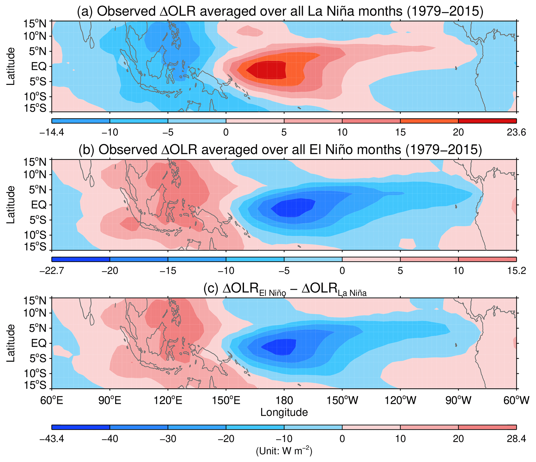
Figure 2Mean OLR deviations from climatology for (a) La Niña and (b) El Niño conditions over the tropical Indian and Pacific oceans. Panel (c) shows differences in the mean OLRA between El Niño and La Niña conditions. The mean composite OLRA and their differences are derived from the datasets provided by NOAA NCEI.
Figure 3Mean SST deviations from climatology for (a) La Niña and (b) El Niño conditions over the tropical Indian and Pacific oceans. Panel (c) shows differences in the mean SSTA between El Niño and La Niña conditions. The mean composite SSTA and their differences are derived from the NOAA ERSSTv5 SST.
In order to test whether the difference patterns of OLRA and SSTA shown in Figs. 2c and 3c are statistically robust, we use [OLRA] and [SSTA] as our sample points to perform two-tailed tests. Figures S1 and S2 in the Supplement demonstrate that the difference patterns are statistically significant at the 5 % significance level.
In the next section, we will evaluate how the ENSO modulates the QBO periods in the E2.2 models and whether those models can realistically capture the contrast in the OLR (and convection) patterns that generally underlies the difference in wave driving of the QBO between warm and cold ENSO conditions.
Now we investigate the ENSO modulation of the QBO period in the ensemble simulations listed in Table 1.
We first calculate the monthly mean anomalies of zonal winds using the method outlined in Sect. 2.3.1. Then we average those monthly mean anomalous zonal winds over the latitudinal belt from 5∘ S to 5∘ N to obtain the monthly QBO winds over the 1871–2013 period at the following seven pressure levels: 70, 50, 40, 30, 20, 15, and 10 hPa.
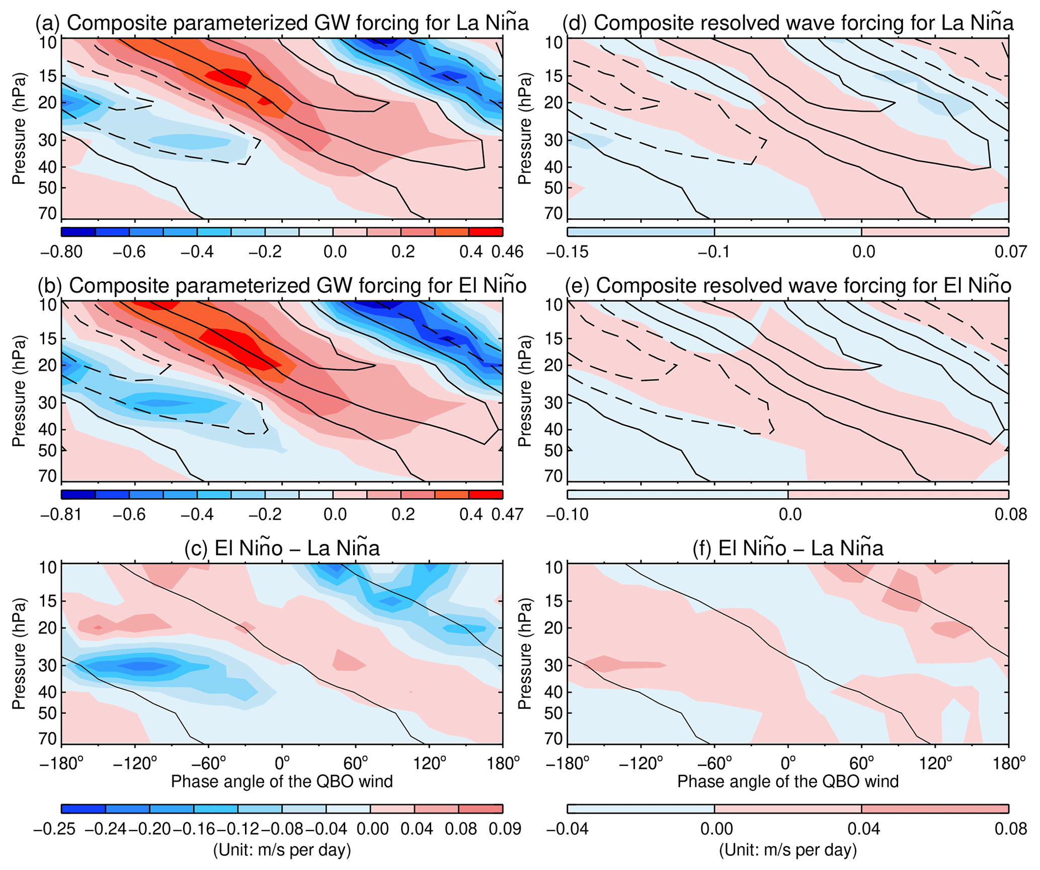
Figure 4Ensemble average of the composite QBO winds simulated by the Coupled–NINT–AP model during La Niña (a, d) and El Niño (b, e) is depicted by contoured black lines where the contour interval is 10 m s−1 with dashed lines denoting negatives and solid lines denoting positives and zero. The location of strong shear zones of the QBO winds during ENSO extremes is delineated by the zero wind contour lines in (c) and (f). For color filled contours, left panels depict the ensemble average of the composite parameterized GW forcing simulated by the Coupled–NINT–AP model averaged from 5∘ S to 5∘ N during La Niña (a) and El Niño (b) and its composite difference between El Niño and La Niña (c), and right panels depict the ensemble average of the composite resolved wave forcing simulated by the Coupled–NINT–AP model during La Niña (d) and El Niño (e) and its composite difference between El Niño and La Niña (f).
As in Sect. 3, we decompose the QBO winds from 10 to 70 hPa over the 1871–2013 period into two leading pairs of EOFs and principal components (PCs). For each of the 19 ensemble simulations listed in Table 1, the first two leading EOFs account for at least 92.9 % of the vertical structure variance, which is comparable to the value derived from the observations discussed in Sect. 3. Since coupled models encounter more difficulties in simulating the ENSO modulations of the QBO (Serva et al., 2020, see their Fig. 4 for more details), we first look into the ensemble simulations from the Coupled–NINT–AP model, which incorporates the most up-to-date cloud parameterization schemes. The red and blue lines in Fig. 1 depict the first two leading EOFs from each of all five Coupled–NINT–AP runs. For each of those five runs, the first two leading EOFs account for at least 93.8 % of the vertical structure variance. The vertical structures of those two EOFs from each Coupled–NINT–AP run are broadly similar to the solid and dashed black lines derived from observations in Fig. 1. The respective vertical structures of the first two leading EOFs are almost identical among all five Coupled–NINT–AP ensemble runs, which is expected because all runs share the same model and differ from each other only in their initial conditions. It is worth noting that the vertical structures of the first two leading EOFs simulated by Coupled–NINT–AP are somewhat different from those observed below the 20 hPa level, because none of the CMIP models could simulate a QBO in the lower stratosphere that was as strong as the observed QBO (Richter et al., 2020). In addition, we find that the vertical structures of the first two leading EOFs from the other three ensemble simulations listed in Table 1 (figures not shown) are comparable to those from the Coupled–NINT–AP runs.
For the ensemble simulations listed in Table 1, we define an El Niño or La Niña event according to the criterion described in Sect. 2.3.1. Similarly, Eq. (3) is used to calculate the instantaneous (i.e., monthly) phase speed of the simulated QBO. For each El Niño or La Niña event, the mean phase speed of the simulated QBO from any individual run listed in Table 1 is obtained by averaging the instantaneous phase speeds of the simulated QBO over the number of months of that event. Accordingly, we have one sample consisting of independent El Niño events and the other consisting of independent La Niña events. In addition, we employ a two-tailed Welch's t test, outlined in Sect. 2.3.2, to examine whether there is a significant difference in the phase speed of the simulated QBO between the El Niño and La Niña population means.
Table 2The ENSO influence on the QBO period. Note: n/a – not applicable.
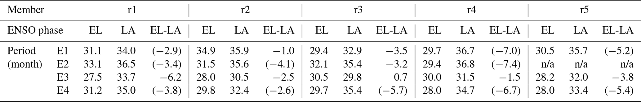
E[1–4] denote the ensemble simulations AMIP-OMA-SP, AMIP-OMA-AP, Coupled-NINT-SP, and Coupled-NINT-AP, respectively. r[1–5] indicate the ensemble members of those simulations. EL and LA are short for El Niño and La Niña, respectively. The numbers in parentheses denote being statistically significantly different from zero at the 5 % significance level.
Table 2 describes how the ENSO influence the QBO period in each member of all ensembles, where E[1–4] represent AMIP–OMA–SP, AMIP–OMA–AP, Coupled–NINT–SP, and Coupled–NINT–AP ensembles, respectively, while r[1–5] indicate its respective member of each ensemble. As we mentioned in Sect. 2.3.1, for the member r1 of E1, i.e., the first run of the AMIP–OMA–SP ensemble, there are 34 El Niño and 30 La Niña events between 1871 and 2013, i.e., N1=34 and N2=30 in Eqs. (5) and (6). Then we obtained the phase speed of the QBO for each episode of those 34 El Niño and 30 La Niña events, from which we derived the mean phase speed of the QBO averaged over the 34 El Niño and 30 La Niña events, respectively. Accordingly, our mean phase speeds of the QBO simulated by r1 of E1 averaged over the El Niño and La Niña events are obtained as 0.202 radians per month and 0.185 radians per month, respectively, and the standard deviations about those mean phase speeds as 0.0345 radians per month and 0.0275 radians per month, respectively. Substituting those numbers into Eqs. (4)–(6) yields ν=61 and t=2.25. Therefore, the phase speed of the QBO simulated by r1 of E1 is statistically significantly greater during El Niño than during La Niña at the 5 % significance level. Accordingly, we register the mean QBO period of 31.1 months (i.e., ) during the El Niño episodes and 34.0 months (i.e., ) during the La Niña episodes as the entries for r1 of E1 in Table 2. Since the phase speeds of the QBO simulated by r1 of E1 are statistically significantly different between the El Niño and La Niña categories at the 5 % significance level, we can regard the QBO periods as being statistically significantly different between El Niño and La Niña episodes and register their difference, −2.9 months, in Table 2 with a pair of parentheses indicating this significance. Similarly, we calculated the QBO periods during ENSO extremes and their difference simulated by every member of all ensembles and registered them in Table 2 where the numbers in the parentheses indicate that the phase speed of the simulated QBO is statistically significantly greater during El Niño than during La Niña at the 5 % significance level.
Table 2 shows that 18 of 19 runs from the four GISS E2.2 models listed in Table 1 can simulate the ENSO modulation of the QBO period discussed in Sect. 3. For each Coupled–NINT–AP ensemble run, the phase speed of the simulated QBO is statistically significantly greater during El Niño than during La Niña at the 5 % significance level. For the AMIP–OMA–SP and AMIP–OMA–AP ensembles, most members also generate a spontaneous QBO whose phase speed is statistically significantly greater during El Niño than during La Niña at the 5 % significance level. Intriguingly, in none of the Coupled–NINT–SP ensemble runs is the phase speed of the simulated QBO statistically significantly different between El Niño and La Niña episodes at the 5 % significance level albeit the contrast in the QBO periods between the two categories simulated by r1 of E3 (i.e., Coupled–NINT–SP) is equal to −6.2 months and greater than that simulated by most members of Coupled–NINT–AP. We will look further into this issue in Sect. 6.
5.1 ENSO modulation of the QBO forcings
Section 4 shows that the ENSO modulation of the QBO period can be simulated by each of the AMIP–OMA–SP, AMIP–OMA–AP, and Coupled–NINT–AP models. The difference in the phase speed of the simulated QBO between ENSO extremes is statistically significant at the 5 % significance level for most of those model runs. For Coupled–NINT–SP, one of its historical runs exhibits an opposite response, namely, the simulated QBO propagates downward slower during El Niño than during La Niña, whereas the other four runs from the identical model configuration do bring about a faster phase speed of the QBO during warm ENSO events. However, no matter whether the difference in the QBO period simulated by Coupled–NINT–SP is positive or negative between ENSO extremes, it is not statistically significant at the 5 % significance level. In this section, we start with investigating how the first three terms in Eq. (7), i.e., the parameterized GW forcing, the resolved wave forcing, and the TEM advection, respond to ENSO extremes and how their evolutions are related with those of the simulated QBO winds.
As shown in Sects. 3 and 4, both the observed and simulated QBO can be very well represented by the trajectory of (PC1(t),PC2(t)) in a linear space spanned by the first two orthonormal EOFs. In other words, at any time t, the QBO wind profile, , is very close to the following linear combination: . Here, the QBO wind, U′, refers to the deseasonalized and smoothed monthly mean zonal winds averaged over the zonal belt from 5∘ S to 5∘ N. We construct the composite fields of the QBO winds, the GW forcing, the resolved wave forcing, and the TEM advection according to the phase angle of the QBO wind profiles. For each month that falls into the El Niño or La Niña category, we use Eq. (2) to calculate the phase angle of the QBO wind profile, each cycle of which over the 1871–2013 period is divided into 24 bins with the bin size of 15∘. Note that if two QBO wind profiles belong in the same bin, they look similar because any one of them can be approximated by the other multiplied by a scalar factor. Therefore, for each of the El Niño and La Niña categories, it is very natural for us to generate the composite QBO winds for that category by averaging all wind profiles in each bin and produce the concomitant composite fields of the GW forcing, the resolved wave forcing, and the TEM advection in the corresponding bin.
Figure 4 depicts the composite fields of the QBO winds (black contours) and parameterized (left panels) and resolved (right panels) wave forcing averaged over all realizations of the Coupled–NINT–AP ensemble. All composite fields in this section have been subjected to the averaging over the latitudinal belt from 5∘ S to 5∘ N.
The ensemble average is achieved on the basis that the respective vertical structures of the first two leading EOFs are almost identical among all five Coupled–NINT–AP ensemble runs as demonstrated in Fig. 1. Both Fig. 4a and b show a characteristic feature of the QBO. Namely, the maximum eastward and westward wave forcing from parameterized GWs are located below and propagate downward with the westerly and easterly QBO jets. Figure 4c reveals the stronger parameterized GW forcing in both eastward and westward shear zones of the QBO winds during El Niño than during La Niña, which gives rise to the faster phase speed of the QBO during warm ENSO episodes than during its cold counterparts. Figure 4d and e show that the relationship between resolved wave forcing and the QBO winds are somewhat more complex. When zonal wind anomalies are close to zero, the coherent and modest resolved westward wave forcing helps the easterly shear zone of the QBO winds to propagate downwards from the 10 hPa level to the 70 hPa level during both the cold and warm ENSO episodes, whereas the coherent and modest resolved eastward wave forcing helps the westerly shear zone of the QBO winds to propagate downwards only from the 20 hPa level to the 70 hPa level during both the cold and warm ENSO episodes. At altitudes above the 20 hPa level, easterly jet cores are modestly weakened by the resolved eastward wave forcing during the two extreme ENSO phases. In particular, Fig. 4f indicates that at altitudes above the 30 hPa level the response of the resolved wave forcing to the ENSO acts to slow down the downward propagation of the QBO during El Niño than during La Niña. However, the parameterized GW forcing shown in Fig. 4 clearly dominates over the resolved wave forcing, which is consistent with the finding of DallaSanta et al. (2021) that the parameterized convective GWs play a dominant role in generating the spontaneous QBO in the GISS E2.2 models.
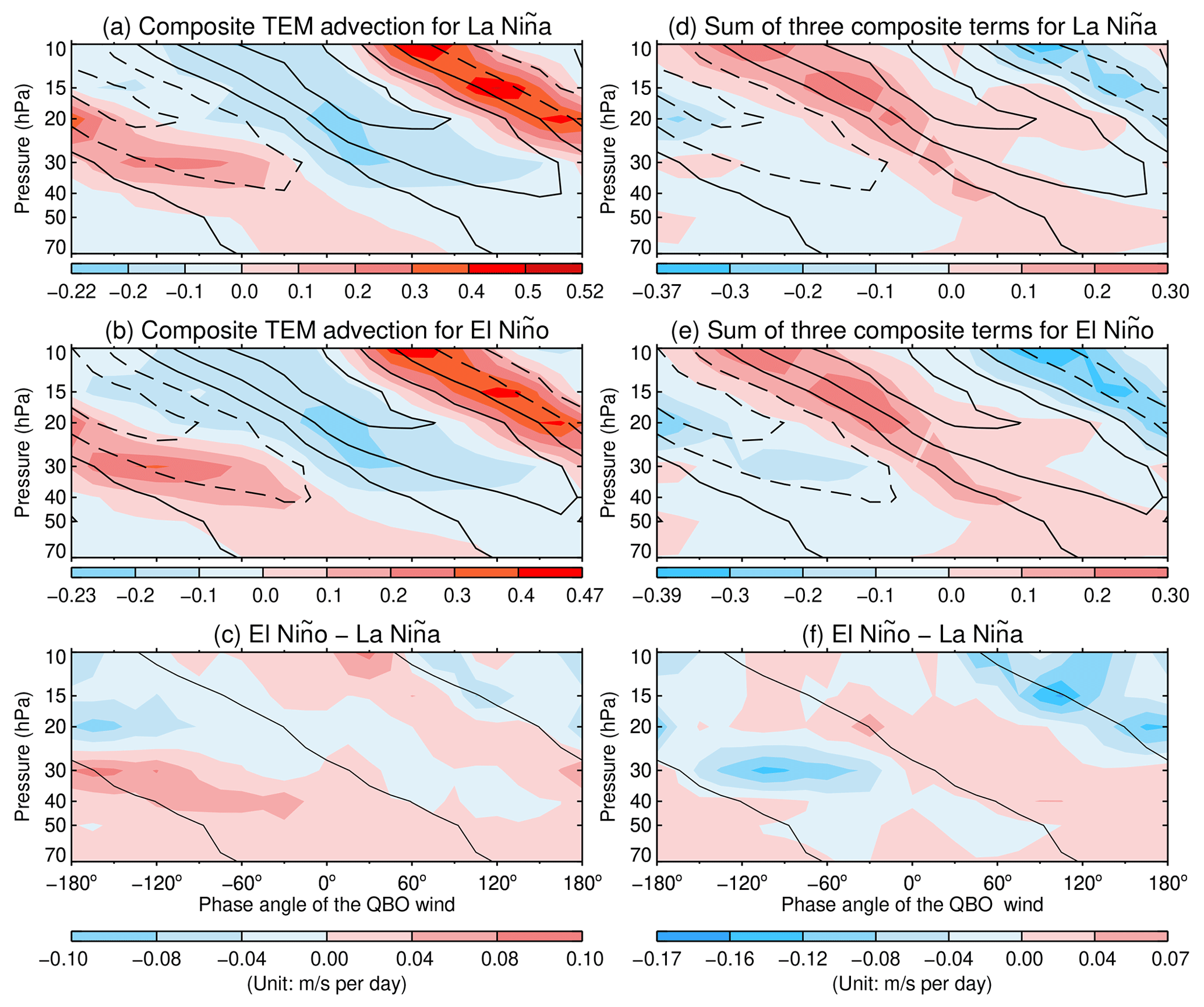
Figure 5The black contour lines are the same as those in Fig. 4. For color filled contours, left panels depict the ensemble average of the composite TEM advection simulated by the Coupled–NINT–AP model averaged from 5∘ S to 5∘ N during La Niña (a) and El Niño (b) and the composite difference between El Niño and La Niña (c); right panels depict the ensemble mean totaling of the composite fields of GW forcing, resolved wave forcing, and TEM advection simulated by the Coupled–NINT–AP model during La Niña (d) and El Niño (e) and the composite difference between El Niño and La Niña (f).
Figure 5a–c depict the composite fields of the QBO winds (black contours) and TEM advection averaged over all realizations of the Coupled–NINT–AP ensemble. Comparing Fig. 5a–c with Fig. 4 reveals that the TEM advection composite is also larger than composite resolved wave forcing in the Coupled–NINT–AP model. Thus, the QBO simulated by this model is intimately related to the parameterized GW forcing and the TEM advection. It is well known that while wave forcing is largely balanced out by the TEM advection in the extratropical stratosphere (Haynes, et al., 1991), tropical wave forcing not only drives internal variabilities of zonal winds but also cancels out the TEM advection in the stratosphere (Scott and Haynes, 1998). Figure 5a and b also show that the maximum positive and negative advective tendencies are located above rather than below and propagate downward with the westerly and easterly QBO jets, thus acting to slow down the downward propagation of the QBO, which is mainly caused by the persistent tropical upwelling and a general feature of the QBO (Giorgetta et al., 2006; Rind et al., 2014). Figure 5c indicates that there exist stronger positive and negative advective tendencies above the westerly and easterly QBO jets during El Niño than during La Niña. In other words, the TEM advection alone leads to a slower phase speed of the QBO during El Niño than during La Niña. This is not surprising because El Niño gives rise to a stronger tropical upwelling in the lower stratosphere (Calvo et al., 2010; Simpson et al., 2011; Domeisen et al., 2019).
Figure 5d–f show the composite QBO winds (black contours) and the composite sum of parameterized GW forcing, resolved wave forcing, and TEM advection averaged over all realizations of the Coupled–NINT–AP ensemble. In other words, the upper, middle, and lower panels depict the sum of the fields shown in all the corresponding panels of Figs. 4 and 5a–c. The pattern of the composite sum is generally determined by the pattern of parameterized GW forcing, even though the latter is more coherent than the former. Thus, we conclude that the shorter QBO period during El Niño simulated by Coupled–NINT–AP is mainly caused by stronger parameterized GW forcing during warm ENSO episodes. We also find that stronger parameterized GW forcing during warm ENSO events is simulated by AMIP–OMA–SP and AMIP–OMA–AP models (figures not shown), which helps us understand why most members from each of those three ensembles generate a spontaneous QBO whose phase speed is statistically significantly greater during El Niño than during La Niña at the 5 % significance level.
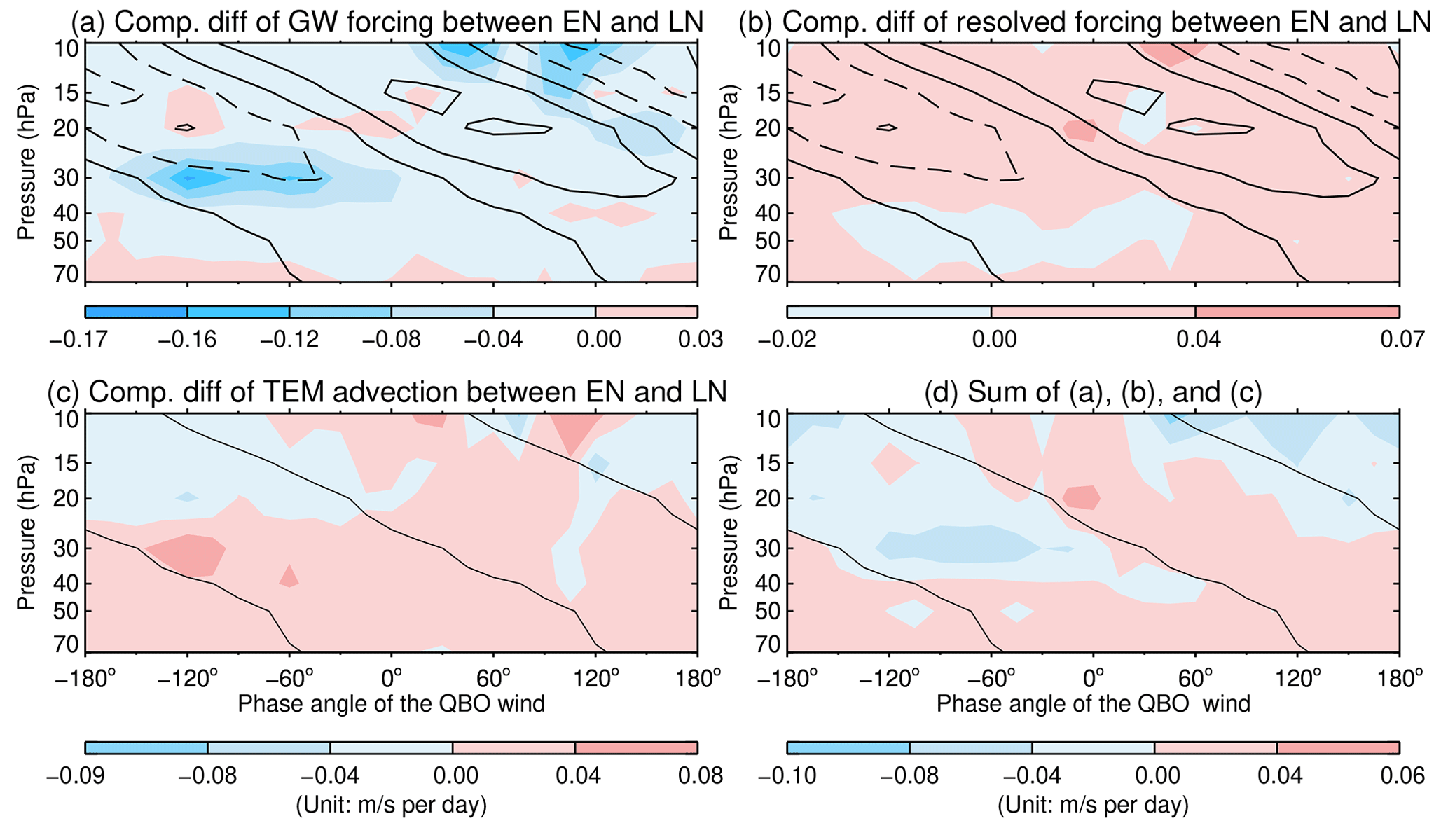
Figure 6Panels (a) and (b) are the same as in Fig. 4c and f except for the Coupled–NINT–SP model. Panels (c) and (d) are the same as in Fig. 5c and f except for the Coupled–NINT–SP model.
Now we explore how ENSO influences parameterized GW forcing, resolved wave forcing, and TEM advection simulated by the Coupled–NINT–SP model, i.e., the remaining model listed in Tables 1 and 2. Contrasting between Figs. 6a and 4c reveals that the ensemble mean composite response to the ENSO of parameterized GW forcing simulated by Coupled–NINT–SP is substantially weaker than that simulated by Coupled–NINT–AP. Although the Coupled–NINT–SP simulations still bring about enhanced westward parameterized GW forcing in the easterly shear zones of the simulated QBO winds during El Niño in contrast to La Niña, the magnitude of the reinforcement is only about two-thirds of that simulated by Coupled–NINT–AP. In particular, in Fig. 6a there is no coherent pattern of enhanced eastward parameterized GW forcing in the westerly shear zones of the QBO winds simulated by Coupled–NINT–SP, which is in glaring contrast to the coherent pattern of positive enhancement shown in Fig. 4c generated from the Coupled–NINT–AP ensemble. Figure 6b and c show that both resolved wave forcing and TEM advection respond to the ENSO weakly and uniformly in the Coupled–NINT–SP ensemble simulations. Combining all three composite fields together, Fig. 6d demonstrates that the ensemble mean of the Coupled–NINT–SP simulations still simulates a coherent but much weaker response to the ENSO of resultant forcing at altitudes above the 40 hPa level, which helps us to explain why only some of the Coupled–NINT–SP ensemble runs can simulate a faster QBO descent rate during El Niño than during La Niña and the ENSO does not make a difference in the phase speed of the QBO that is statistically significant at the 5 % significance level in any of those Coupled–NINT–SP runs.
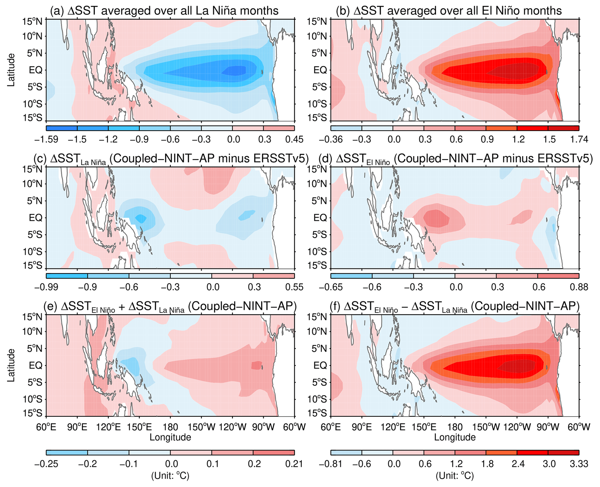
Figure 7Ensemble mean of the composite SSTA from the Coupled–NINT–AP runs averaged over all La Niña (a) and El Niño (b) months, respectively, over the 1871–2013 period. Differences from observations are shown in (c) and (d). The sum and difference of model derived El Niño and La Niña SSTA are shown in (e) and (f), respectively.
5.2 ENSO modulation of the generation and propagation of parameterized gravity waves
A natural question that arises is how the parameterized GW forcing relates to the SSTA of ENSO extremes specified in or simulated by the GISS E2.2 models listed in Table 1. Figure 7a and b show the ensemble averages of the composite SSTA averaged over all La Niña and El Niño months, respectively, over the 1871–2013 period simulated by Coupled–NINT–AP. Comparing Fig. 7a and b with Fig. 3a and b reveals that the amplitude of the ENSO simulated by Coupled–NINT–AP is larger than the observed ENSO. Figure 7c and d show the differences between the simulated SSTA arising from the ENSO events shown in Fig. 7a and b and the observed SSTA shown in Fig. 3a and b, indicating that the largest discrepancies occur over the western and eastern equatorial Pacific. Figure 7a and b also demonstrate that the model has a capability to simulate the ENSO amplitude asymmetry (Cane and Zebiak, 1987; Yu and Mechoso, 2001), namely, the amplitudes of the ENSO are relatively larger during warm episodes than during cold episodes. As in Fig. 3 of Zhao and Sun (2022), Fig. 7e depicts the sum of the composite SSTA shown in Fig. 7a and b that they used to characterize the ENSO amplitude asymmetry, whereas Fig. 7f shows their difference. Their Fig. 3 reveals that most CMIP6 models cannot simulate the pattern of a positive residual in the sum of the composites of ENSO extremes in the tropical eastern Pacific. Further comparison between Fig. 3 in Zhao and Sun (2022) and Fig. 7e indicates that the ENSO amplitude asymmetry simulated by Coupled–NINT–AP is only about 50 % of that simulated by the GISS-E2-1-H model discussed in their study whose ENSO amplitude asymmetry is comparable to the observed amplitude asymmetry.
Since this study is chiefly concerned with the ENSO modulation of the QBO period, we focus on the ensemble mean difference between the composite SSTA of ENSO extremes, which can be interpreted as the trough-to-crest amplitude of the ENSO cycle. Comparing Fig. 8a with Fig. 3c indicates that the trough-to-crest ENSO amplitude derived from the HadISST1 dataset over the 1871–2013 period is somewhat smaller than that derived from the ERSSTv5 dataset over the 1953–2015 period, which is consistent with the finding by Grothe et al. (2019) that the increase in the ENSO variability is statistically significant (> 95 % confidence) from the preindustrial to recent era, no matter whether the latter is defined by the previous 30, 50, 75, or 100 years before 2016. Figures 7f and 8 also reveal that the ENSO amplitude simulated by Coupled–NINT–AP is substantially greater than that simulated by Coupled–NINT–SP, which was previously revealed in Rind et al. (2020). The tendency to generate stronger ENSO oscillations means that the Coupled-NINT-AP runs will also more readily exceed the ±0.5 ∘C criteria for El Niño and La Niña events, and the Coupled–NINT–AP runs do simulate more ENSO events over the 1871–2013 period than the Coupled–NINT–SP runs as indicated in Sect. 2.3.1. Figure 8 further shows that the ENSO amplitude simulated by Coupled–NINT–SP is noticeably greater than those specified in the AMIP–OMA–SP and AMIP–OMA–AP models (which, being derived from observations, are identical), even though it is substantially weaker than that simulated by Coupled–NINT–AP.
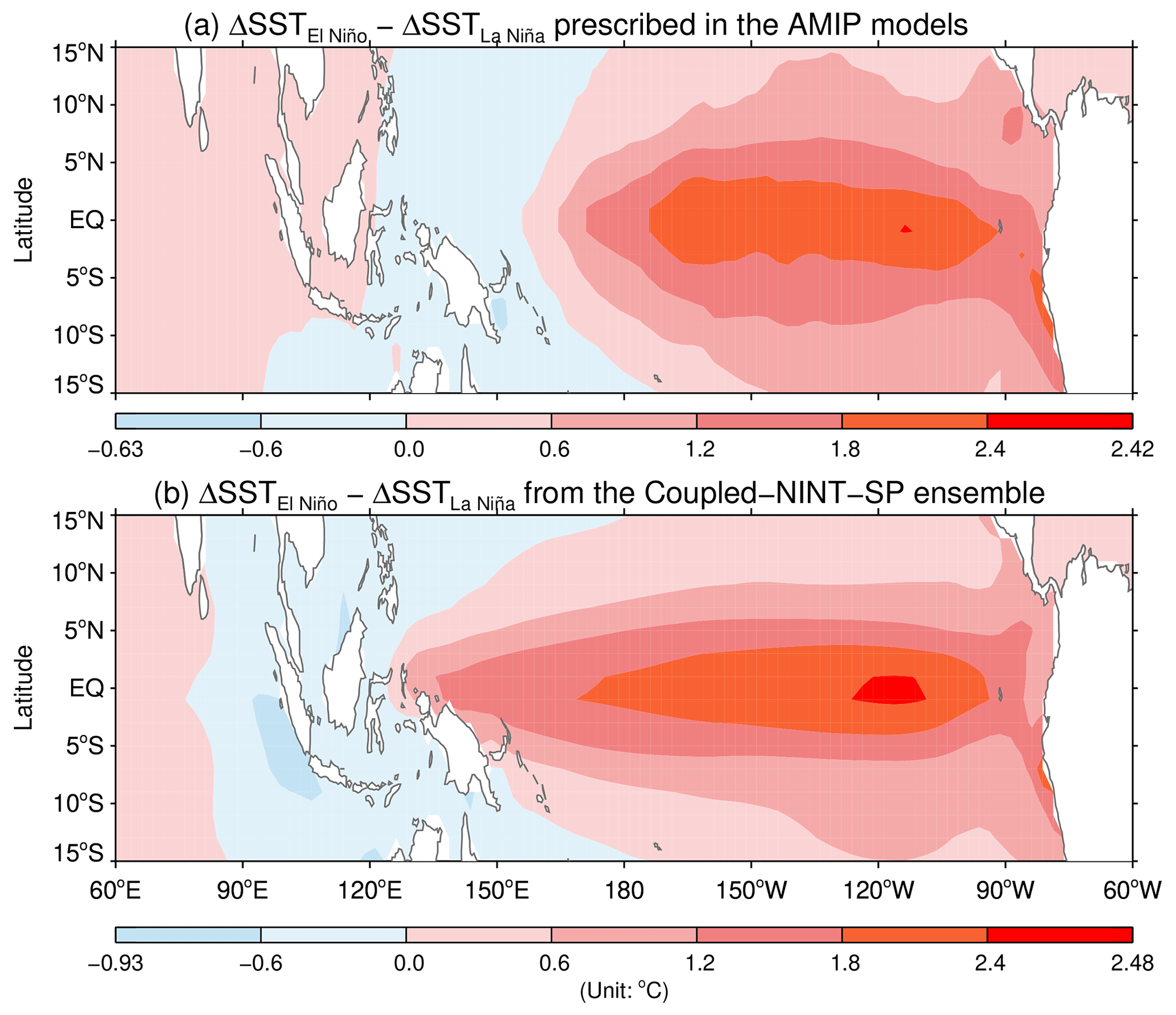
Figure 8Difference in the composite SSTA between El Niño and La Niña over the 1871–2013 period specified in the AMIP–OMA–SP and AMIP–OMA–AP models (a) and that simulated by the Coupled–NINT–SP model (b).
We also ascertain that the Hadley circulation simulated by each of the four models listed in Table 1 strengthens and weakens during warm and cold ENSO episodes, respectively (figure not shown), which is consistent with the findings of Oort and Yienger (1996).
Schirber (2015) discovered that the parameterized GW mean momentum source is about 15 % larger in the El Niño ensemble than in the La Niña ensemble because the El Niño leads to enhanced precipitation and convective heating. Similarly, we calculate the absolute value of convective momentum fluxes (ACMF) at the source altitude and composite the ACMF anomalies averaged over the latitudinal belt between 5∘ S and 5∘ N from El Niño and La Niña categories, respectively, over the 1871–2013 period. Figure 9 shows the composite difference in the equatorial mean ACMF anomalies between El Niño and La Niña over the 1871–2013 period, indicating that the absolute momentum fluxes at the source levels over the equatorial belt is larger during El Niño episodes than during La Niña episodes for each of 19 runs listed in Table 1. This finding is consistent with that of Geller et al. (2016b), Alexander et al. (2017), and Kang et al. (2018), namely, both convective GW momentum fluxes and convective GW wave forcing are generally stronger during El Niño than during La Niña in the equatorial region. The ensemble mean difference in the absolute momentum fluxes at the source levels averaged over that equatorial belt between El Niño and La Niña is obtained as 0.07, 0.15, 0.10, and 0.12 mPa for AMIP–OMA–SP, AMIP–OMA–AP, Coupled–NINT–SP, and Coupled–NINT–AP, respectively. Note that these composite differences in ACMF between El Niño and La Nina translate into ACMF being about 10 %–20 % larger in the El Niño ensembles than in the La Niña ensembles and thus agree with the Schirber (2015). Since the QBO period is inversely dependent on the momentum flux (Plumb, 1977), the differences in equatorial absolute momentum fluxes at the source altitude contribute to shortening and lengthening of the simulated QBO period during warm and cold ENSO phases, respectively.
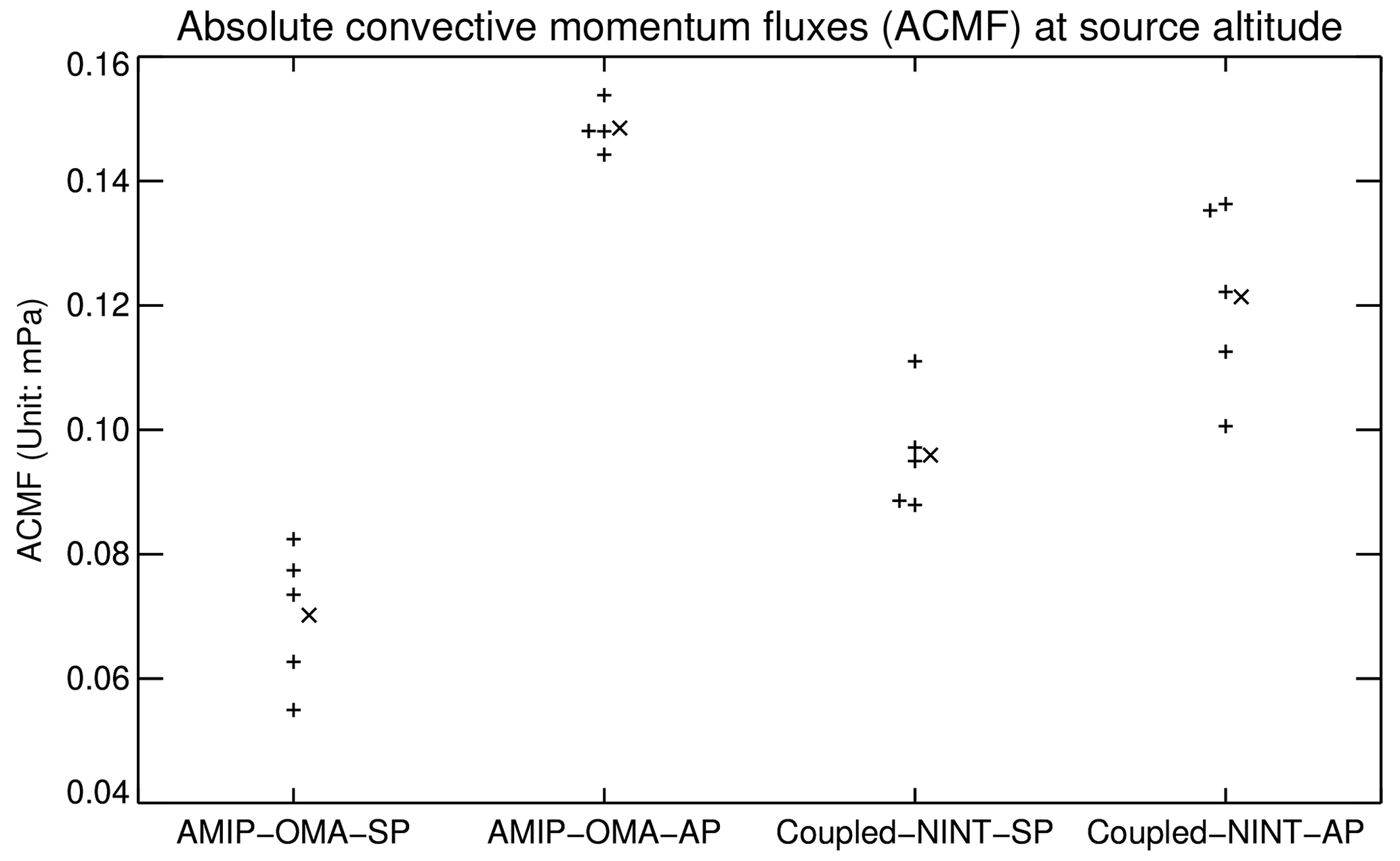
Figure 9Difference in the composite ACMF anomalies at the source altitude averaged over the 5∘ S to 5∘ N latitudinal belt between El Niño and La Niña over the 1871–2013 period. Plus symbol (+) denotes the difference from individual runs and cross symbol (×) represents each ensemble mean difference. Some symbols are slightly shifted leftward or rightward to avoid overlapping with other symbols.
Figure 3 shows that the locations of the warmest SSTs shift from the maritime continent during La Niña episodes to the central and eastern equatorial Pacific during El Niño episodes. Since strong convective activities over tropical oceans are generally located above the regions where the SSTs exceed 26–28 ∘C (Graham and Barnett, 1987; Zhang, 1993), strong convective activities also shift eastward from cold to warm ENSO phases, as illustrated in Fig. 2. Using satellite data, the climatological study by Sullivan et al. (2019) demonstrated that the occurrence of organized deep convection during El Niño events increases 3-fold in the central and eastern Pacific and decreases 2-fold outside of these regions, in contrast to that during La Niña events. It is well established that the Walker circulation strengthens during La Niña and weakens during El Niño (Bjerknes, 1969).
Next, we construct the equatorial zonal winds as the zonal winds averaged from 5∘ S to 5∘ N. Then we define the equatorial winds during La Niña and El Niño as the equatorial winds averaged over all months that fall into the La Niña and El Niño categories, respectively. Figure 10 illuminates that the Walker circulation derived from ERA5 reanalysis during El Niño is substantially weaker than its counterpart during La Niña over the equatorial Pacific and the eastern equatorial Indian Ocean. Particularly in the upper equatorial troposphere, the westerlies above the central and eastern Pacific during El Niño episodes are decreased by more than 50 % as compared with those during La Niña episodes, whereas the easterlies above the equatorial Indian Ocean and the maritime continent during El Niño conditions are weakened by more than 30 % as compared with those during La Niña conditions. Kawatani et al. (2019) argue that the weaker upper tropospheric winds during El Niño episodes enable a greater amount of GW momentum fluxes to be transferred from the troposphere into the stratosphere because fewer GWs are filtered out. This argument assumes critical-level absorption of otherwise weakly damped, vertically propagating GWs, which was adopted by Lindzen and Holton (1968). The weaker Walker circulation leads to a shorter QBO period during El Niño, whereas the stronger Walker circulation results in a longer QBO period during La Niña.
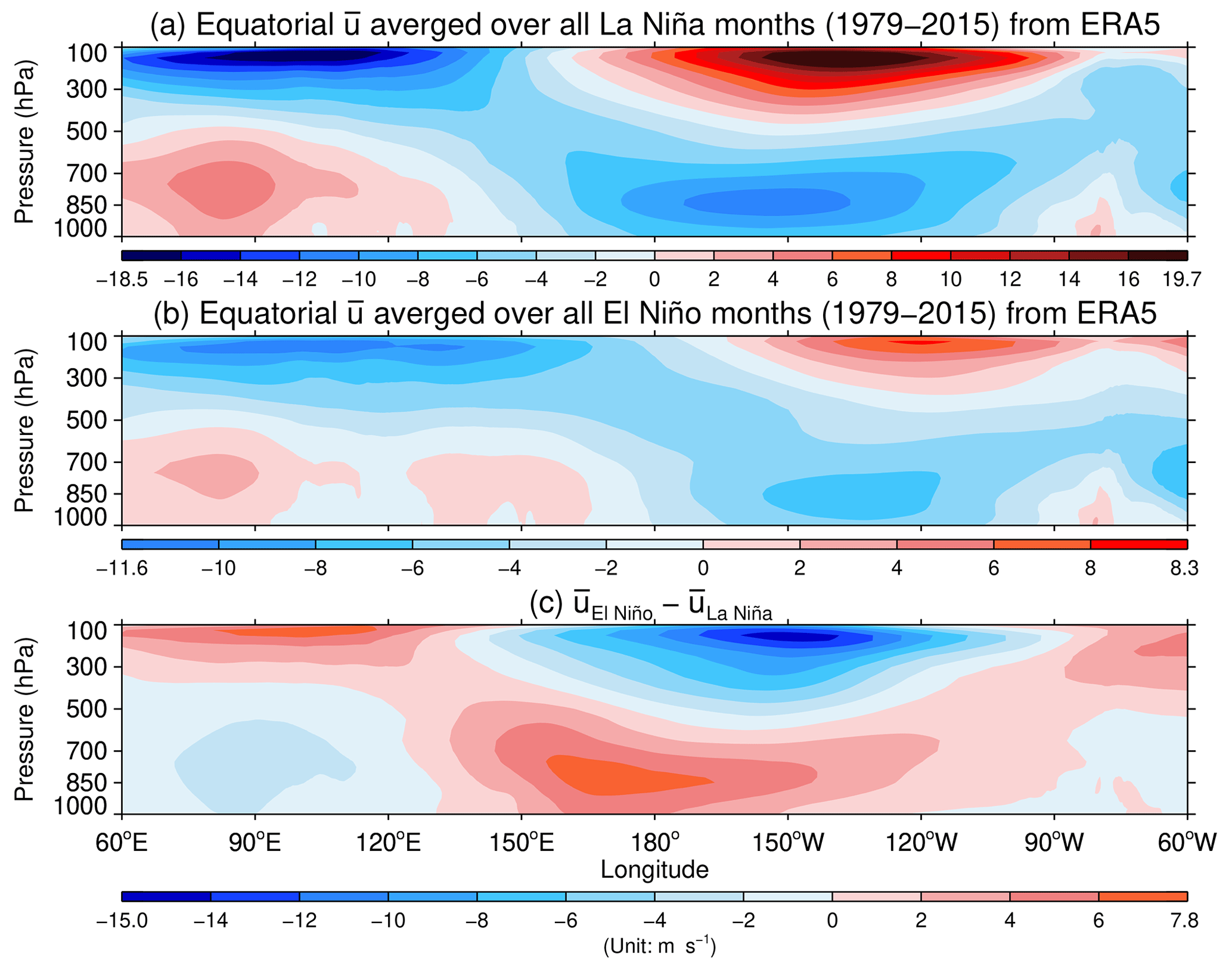
Figure 10Zonal winds from ERA5 averaged from 5∘ S to 5∘ N that are further averaged over all La Niña (a) and El Niño (b) months between 1979 and 2015, respectively, and their differences (c).
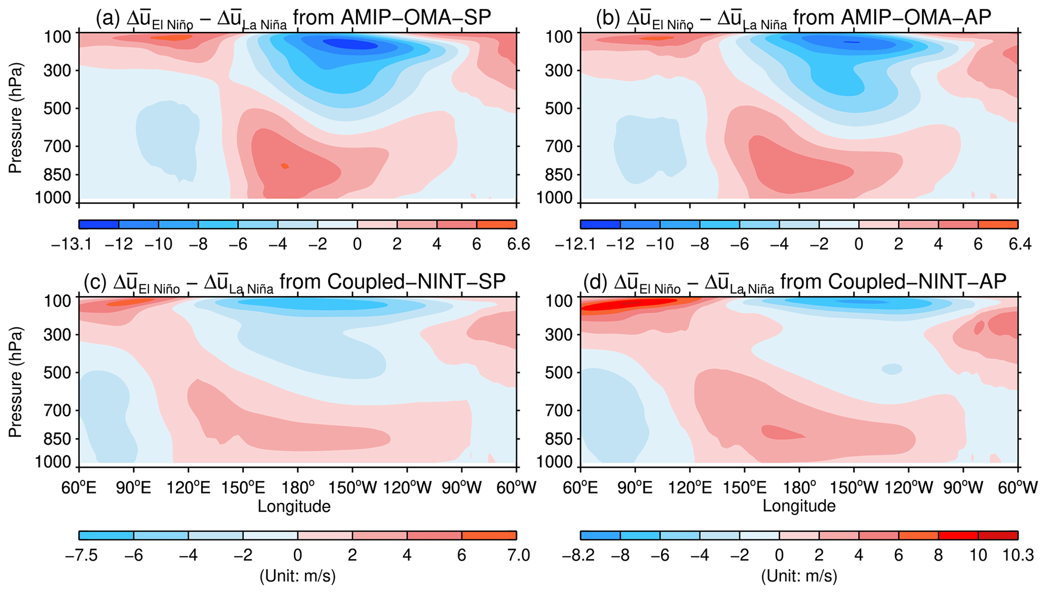
Figure 11Same as Fig. 10c but for the ensemble averages of the composite difference in zonal wind anomalies between El Niño and La Niña simulated by AMIP–OMA–SP (a), AMIP–OMA–AP (b), Coupled–NINT–SP (c), and Coupled–NINT–AP (d).
Figure 11 depicts the ensemble mean composite difference in the equatorial zonal wind anomalies between warm and cold ENSO extremes simulated by the E2.2 models listed in Table 1. The patterns of the simulated wind anomalies shown in Fig. 11 are very similar to those derived from the ERA5 reanalysis shown in Fig. 10c. Namely, the weakened Walker circulation simulated by the E2.2 models during El Niño episodes results in weaker upper tropospheric westerlies over the central and eastern equatorial Pacific and weaker upper tropospheric easterlies over the maritime continent and equatorial Indian Ocean while the intensified Walker circulation simulated by the E2.2 models during La Niña episodes leads to stronger upper tropospheric westerlies over the central and eastern equatorial Pacific and stronger upper tropospheric easterlies over the maritime continent and equatorial Indian Ocean. The difference in the wind filtering of upward propagating GWs causes a greater transfer of GW momentum fluxes into the tropical stratosphere during El Niño episodes than during La Niña episodes, leading to a shorter QBO period during El Niño events than during La Niña events. Figure 11 reveals that the maximum contrast in the upper tropospheric zonal winds between warm and cold ENSO extremes simulated by two AMIP models, i.e., AMIP–OMA–SP and AMIP–OMA–AP, reaches −13.1 and −12.1 m s−1, respectively, over the central and eastern equatorial Pacific, and attains 6.6 and 6.4 m s−1, respectively, over the maritime continent and equatorial Indian Ocean. Those maximum contrasts are somewhat smaller than what is derived from the ERA5 reanalysis shown in Fig. 10, namely, −15.0 m s−1 over the central and eastern equatorial Pacific and 7.8 m s−1 over the maritime continent and equatorial Indian Ocean. However, the maximum contrast in the upper tropospheric zonal winds over the central and eastern equatorial Pacific between warm and cold ENSO extremes simulated by two coupled ocean–atmosphere models, i.e., Coupled–NINT–SP and Coupled–NINT–AP, only reaches −7.5 and −8.2 m s−1, respectively, and thus is substantially smaller than that derived from the ERA5 reanalysis. Meanwhile, the maximum contrast in the upper tropospheric zonal winds over the maritime continent and equatorial Indian Ocean between warm and cold ENSO extremes simulated by those two coupled models reaches 7.0 and 10.3 m s−1, respectively, which is slightly smaller than and somewhat larger than the observed values, respectively.
The comparison of the observed and simulated changes in the Walker circulation between warm and cold ENSO extremes shown in Figs. 10 and 11 can both account for a shorter QBO period simulated by all GISS E2.2 models and explain why the two AMIP models can better capture the ENSO modulation of the QBO period than the Coupled–NINT–SP model as indicated in Table 2. However, it can neither explain why the Coupled–NINT–AP model can capture the ENSO modulation of the QBO period as two AMIP models nor illuminate why the coupled model with the “altered physics” (i.e., Coupled–NINT–AP) performs better than the coupled model with the “standard physics” (i.e., Coupled–NINT–SP). Further comparing the simulated SST changes between warm and cold ENSO extremes shown in Figs. 7 and 8 hints that the unduly amplified ENSO in the coupled AP runs holds the key to those unsettled issues which are detailed next.
Using a large ensemble of multiple climate models, Serva et al. (2020) discovered that the AMIP historical runs generally better capture the ENSO modulation of the QBO period than the coupled ocean–atmosphere historical simulations. In particular, among a few coupled ocean–atmosphere models that do, to various extents, capture the ENSO modulation of the QBO period, the common feature is that each of them can largely simulate the observed OLR anomaly pattern shown in Fig. 2c, albeit the magnitudes of those simulated OLRA from their historical runs are roughly 50 % stronger than the observed OLRA. (For more details, refer to Fig. 8 in Serva et al., 2020.) For the sake of comparison, we construct the ensemble mean composite difference in the OLRA between warm and cold ENSO extremes in the same way we constructed the ensemble mean composite difference in the zonal wind anomalies depicted in Fig. 11.
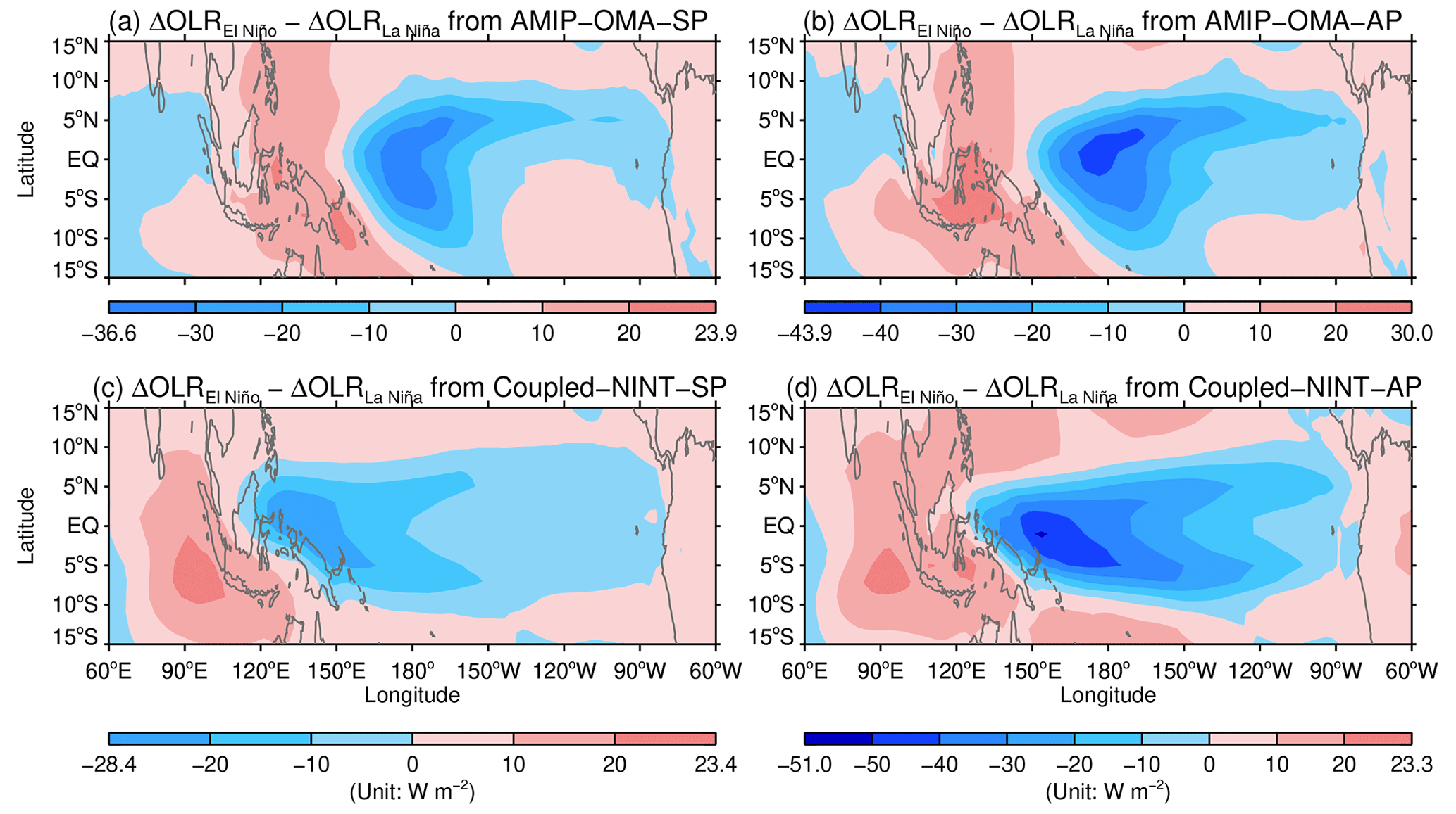
Figure 12Same as Fig. 11 but for the ensemble averages of the composite difference in OLRA between El Niño and La Niña simulated by AMIP–OMA–SP (a), AMIP–OMA–AP (b), Coupled–NINT–SP (c), and Coupled–NINT–AP (d).
Figure 12a and b show that the patterns of the OLRA simulated by AMIP–OMA–SP and AMIP–OMA–AP largely resemble the observed pattern shown in Fig. 2c. Although the pattern simulated by AMIP–OMA–AP matches better with the observed pattern, the convective activities during El Niño episodes simulated by AMIP–OMA–SP and AMIP–OMA–AP are apparently inadequate over the region where the upper tropospheric westerlies weaken most conspicuously during the warm ENSO extremes shown in Fig. 11a and b, respectively. Thus, although the contrast in the wind filtering of GWs between El Niño and La Niña episodes simulated by the two AMIP E2.2 models are comparable to the observed episodes, the difference in the GW momentum flux transferred into the equatorial stratosphere between warm and cold ENSO extremes may well be smaller than the observed difference with the correct SSTs. This partly explains why the contrast between the observed mean QBO period during El Niño episodes (i.e., 25.6 months) and the observed mean QBO period during La Niña episodes (i.e., 34.3 months) is higher than that simulated by the two AMIP models shown in Table 2 (i.e., E1 and E2 in Table 2). As exhibited by the coupled model capable of simulating the ENSO modulation of the QBO period, Fig. 12d shows that the contrast in the OLRA between warm and cold ENSO extremes simulated by Coupled–NINT–AP is apparently sharper than the observed contrast shown in Fig. 2c. In particular, the tropical convection in the central and eastern Pacific during El Niño episodes simulated by Coupled–NINT–AP is both more extensive and more intensive than that simulated by the two AMIP models shown in Fig. 12a and b, which is consistent with the fact that the composite contrast in the SSTA simulated by Coupled–NINT–AP shown in Fig. 7d is substantially sharper than that prescribed in the two AMIP models shown in Fig. 8a. Thus, even though the wind filtering of GWs during El Niño episodes simulated by Coupled–NINT–AP shown in Fig. 12d is significantly smaller than that simulated by AMIP–OMA–SP and AMIP–OMA–AP shown in Fig. 12a and b, respectively, the combined effect of the lower contrast in the wind filtering and the higher contrast in the amount of GW momentum fluxes generated by convective activities between warm and cold ENSO extremes over the central and eastern tropical Pacific results in a comparable ENSO modulation of the QBO period simulated by Coupled–NINT–AP to that simulated by the two AMIP models as illustrated in Table 2.
Finally, comparing Fig. 12c with Fig. 2c and the other three panels in Fig. 12 reveals that convective activities during the warm ENSO phase simulated by the Coupled–NINT–SP model are substantially weaker than both the observed convective activities and those simulated by the other three models listed in Table 1. Combining the small composite OLR difference shown in Fig. 12c and the small difference in the wind filtering shown in Fig. 8c between warm and cold ENSO extremes over the central and eastern equatorial Pacific results in a low contrast in GW forcing between the warm and cold ENSO phases shown in Fig. 6a, which, short of the compensating effect of the excessively amplified ENSO in Coupled–NINT–AP ensemble runs, should lead to a relatively weaker ENSO modulation of the QBO period simulated by the Coupled–NINT–SP model as illustrated in Table 2. However, this is not the whole story, and we will return to this subject in the next section1.
Both Kawatani et al. (2019) and Serva et al. (2020) pointed out that a relatively high horizontal resolution is necessary to simulate the ENSO modulation of the QBO period. Employing an earth system model with T42 (∼ 2.79∘) horizontal resolution, Kawatani et al. (2019) further demonstrated that the ENSO modulation of the QBO could not be simulated with their fixed GW sources. Serva et al. (2020) also pointed out that the reliance on stationary parameterizations of GWs is partly responsible for failing to simulate the observed modulation of the QBO by the ENSO in current climate models.
Rind et al. (1988) implemented various interactive GW sources in the GISS climate models. With the momentum flux of the parameterized convective waves dependent on the convective mass flux, buoyancy frequency and density at the top of the convective region, wind velocity averaged over the convective layers, and with a horizontal resolution of 2∘ latitude by 2.5∘ longitude, all four versions of the GISS E2.2 models in this study can simulate the ENSO modulation of the QBO period to various degrees. For each of 19 runs conducted in this study, the absolute momentum fluxes at the source levels over the equatorial belt are larger during El Niño episodes than during La Niña episodes, leading to a shorter and longer QBO period, respectively.
Realistic simulation of the ENSO modulation of the QBO periods entails realistic simulation of both the ENSO and the QBO. With the realistic SSTs specified, both the composite difference in the Walker circulation and the composite OLR difference between warm and cold ENSO extremes simulated by the two AMIP E2.2 models are close to the observed extremes. Since the AMIP model with the “altered physics” performs better than that with the “standard physics” as far as the simulated OLR is concerned, the ensemble mean difference in the QBO period between La Niña and El Niño episodes (i.e., ∼ 4.5 months) simulated by AMIP–OMA–AP is larger than that simulated by AMIP–OMA–SP (i.e., ∼ 3.9 months), which indicates that a convective parameterization scheme is important not only for simulating the resolved waves, as pointed out by Horinouchi et al. (2003) and Lott et al. (2014), but also for parameterizing GWs. However, the convective activities simulated by both AMIP E2.2 models are still inadequate over the central and eastern equatorial Pacific as compared with the observed convective activities, which may partly account for why the ensemble mean differences in the QBO period between La Niña and El Niño episodes simulated by both AMIP models are smaller than the observed difference (i.e., ∼ 8.7 months).
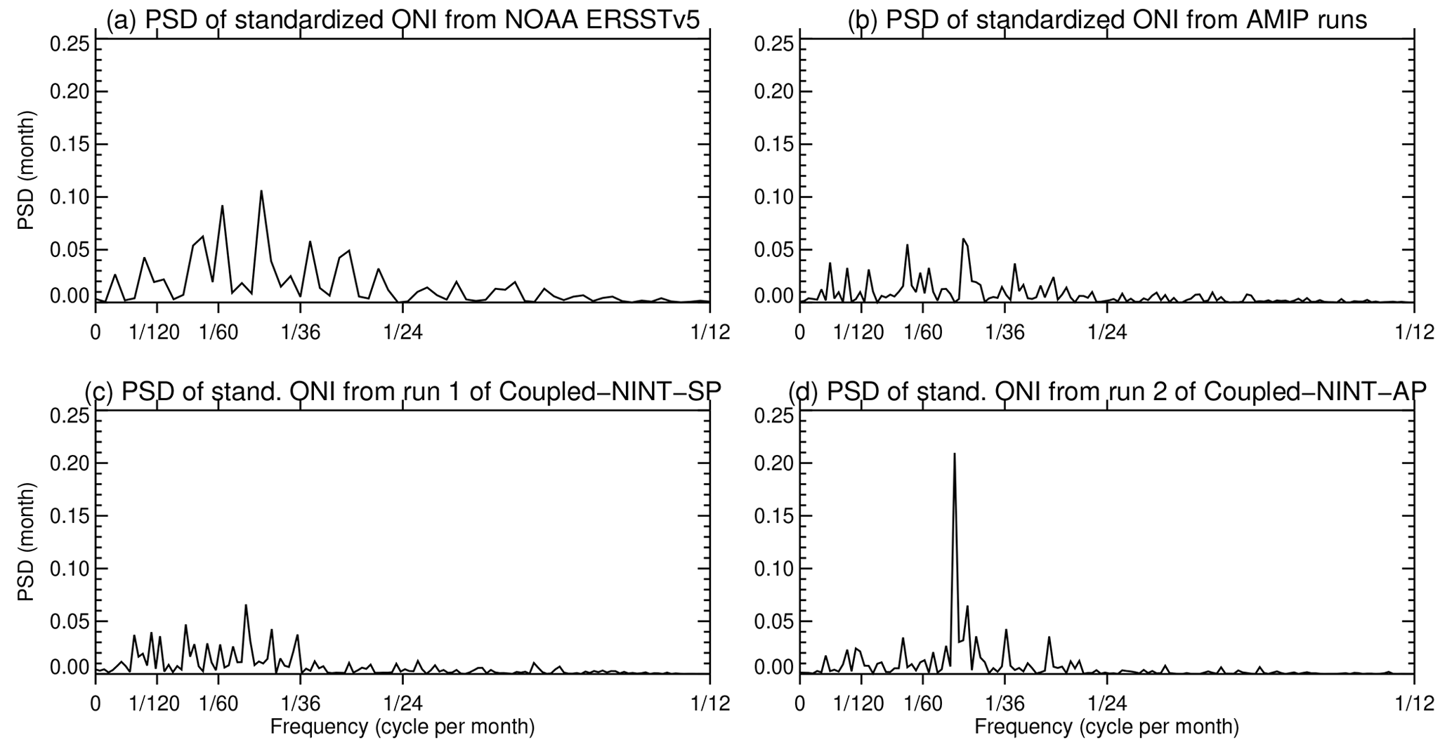
Figure 13Power spectral densities (PSD) of the standardized ONI between 1953 and 2015 derived from the NOAA ERSSTv5 SST (a), of standardized ONI between 1871 and 2013 derived from the HadISST1 dataset as used in the AMIP runs (b), of standardized ONIs between 1871 and 2013 simulated by the first realization of Coupled–NINT–SP (c), and the second realization of Coupled–NINT–AP (d), respectively.
Although the simulated Walker circulation associated with the ENSO cycle is comparable among the two coupled ocean–atmosphere models in this study, the E2.2 model with the “standard physics” performs well in its simulated SSTs, which are very close to the observed SSTs, whereas the ENSO amplitudes simulated by the other model with the “altered physics” are substantially greater than the observed ENSO amplitudes. Yet the model with the “standard physics” not only fails to properly simulate the shift of the strongest convection from the maritime continent during La Niña to the central and eastern equatorial Pacific during El Niño, but also grossly fails to simulate the sufficient amplitude of the OLR concomitant with the ENSO cycle. The weaker response of the Walker circulation and convective activities to the ENSO cycle together with the dislocated centers of convection concomitant to cold and warm ENSO extremes leads to the smallest ensemble mean difference in the QBO period between La Niña and El Niño episodes (i.e., ∼ 2.7 months) simulated by the Coupled–NINT–SP model. The weaker variation in the Walker circulation and the excessive change in convection compensate to give an impression of realistically simulating the ENSO modulation of the QBO period by the other model with the “altered physics”, i.e., Coupled–NINT–AP, with its ensemble mean differences in the QBO period between La Niña and El Niño episodes being ∼ 4.8 months. However, it is worth pointing out that we do not regard that model as the best among the four models listed in Table 1 because the relatively satisfactory results are achieved in a compensatory, and thus unrealistic, way. Serva et al. (2020) conducted both the atmosphere-only and coupled historical simulations and found that the trough-to-crest amplitudes of the OLR associated with the ENSO cycle are two times larger than the observed amplitudes for a few models that capture relatively well the ENSO modulation of the QBO period, which together with our results suggests that the parameterized convection is a linchpin of realistically simulating the ENSO, the QBO, and the ENSO modulation of the QBO.
Intriguingly, the simulated difference in the QBO period between La Niña and El Niño is 6.2 months from the first realization simulated by Coupled–NINT–SP. However, it is not statistically significant at the 5 % significance level. Meanwhile, the differences in the QBO period between La Niña and El Niño from most of the realizations simulated by Coupled–NINT–AP are apparently less than 6.2 months but are all statistically significant. To gain a deeper insight, we calculate the frequency power spectra of standardized ONIs derived from the observed and simulated SSTs. Figure 13a depicts the power spectral densities (PSD) of standardized ONI between 1953 and 2015 derived from the NOAA ERSSTv5 SST and Fig. 13b delineates the PSD of standardized ONI between 1871 and 2013 derived from the HadISST1 dataset as used in the AMIP runs. Figure 13a and b show that although ENSO accounts for the lion's share of SST variabilities, there is a good amount of SST variabilities on the decadal and multidecadal timescales. Figure 13d illustrates the PSD of standardized ONI between 1871 and 2013 simulated by the second realization of Coupled–NINT–AP, which demonstrates that the ENSO overwhelmingly dominates over any other noises in SST variabilities simulated by those E2.2 models with the “altered physics”. Furthermore, Fig. 13c shows the PSD of standardized ONI between 1871 and 2013 simulated by the first realization of Coupled–NINT–SP. Apparently, the SST variabilities simulated by the E2.2 model with the “standard physics” are comparable to the observed SST variabilities and, thus, more realistic. The smaller ratio of the ENSO signal to the noise simulated by the first realization of Coupled–NINT–SP and the much larger ratio simulated by the second realizations of the E2.2 models with “altered physics” explain why the difference of 6.2 months in the QBO period between La Niña and El Niño from the former is not statistically significant, whereas the differences of 2.6 and 4.8 months from the latter are statistically significant as shown in Table 2.
The rich spectrum of internal variabilities simulated by Coupled–NINT–SP, to a large degree, reflects the observed variabilities shown in Fig. 13a and b. Those large internal variabilities likely underlie why one of the historical runs simulated by Coupled–NINT–SP gives rise to a slower mean QBO phase speed during El Niño than during La Niña, whereas the other four runs from Coupled–NINT–SP do simulate a faster phase speed of the QBO during warm ENSO events. Kawatani et al. (2019) conducted two 100-year experiments: one for a perpetual El Niño condition and the other for a perpetual La Niña condition. Their Fig. 3 shows that although the long-term mean QBO period from the El Niño run is shorter than that from the La Niña run, this is not the case for each individual year. This is because various internal variabilities exert their influence over the QBO period.
None of the E2.2 configurations robustly simulate an ENSO modulation of QBO amplitude, consistent with the weaker signal present in observations (Yuan et al., 2014). It is not surprising because our observational analyses show that the ENSO modulation of the QBO amplitude is not statistically significant at the 95 % confidence level. In order to realistically simulate the ENSO modulation of the QBO, various aspects of climate models, such as SSTs, the Walker circulation, the parameterizations of convection, and GWs, need to be further improved, which is fortunately ongoing under the auspices of the SPARC Quasi-Biennial Oscillation initiative (Butchart et al., 2018).
The monthly mean zonal winds from Free University of Berlin are obtainable from https://www.geo.fu-berlin.de/en/met/ag/strat/produkte/qbo/index.html (Naujokat, 1986). The NOAA ERSSTv5 SST is obtainable from https://doi.org/10.7289/V5T72FNM (Huang et al., 2017b). The NCEI OLR is obtainable from https://doi.org/10.7289/V5W37TKD (Lee and NOAA CDR Program, 2018). The ERA5 monthly mean zonal winds are obtainable from the ECMWF C3S at Climate Data Store: https://doi.org/10.24381/cds.6860a573 (Hersbach et al., 2023, 2020). The Coupled–NINT–AP outputs are available from the Earth System Grid Federation (ESGF; https://doi.org/10.22033/ESGF/CMIP6.2081, NASA/GISS, 2019). The data used in this paper from the other three E2.2 models are accessible at https://doi.org/10.5281/zenodo.8360291 (Zhou, 2023).
Figures S1–S5 are supplementary to Figs. 2–6, respectively. Figure S6 is supplementary to Fig. 8. Figures S7–S9 are supplementary to Figs. 10–12, respectively. The supplement related to this article is available online at: https://doi.org/10.5194/acp-24-509-2024-supplement.
Conceptualization: CO, TZ, KJD, DHR, GAS, GR. Formal analysis: TZ, KJD, CO, DHR, JAJ, LN, GAS, GR. Funding acquisition: GAS. Investigation: TZ, KJD, CO, DHR, JAJ, LN, GAS, GR.
The contact author has declared that none of the authors has any competing interests.
Publisher’s note: Copernicus Publications remains neutral with regard to jurisdictional claims made in the text, published maps, institutional affiliations, or any other geographical representation in this paper. While Copernicus Publications makes every effort to include appropriate place names, the final responsibility lies with the authors.
Climate modeling at GISS is supported by the NASA Modeling, Analysis and Prediction Program, and resources supporting this work were provided by the NASA High-End Computing (HEC) Program through the NASA Center for Climate Simulation (NCCS) at Goddard Space Flight Center. The authors thank three anonymous reviewers for their constructive comments, which led to a significantly improved paper.
This research has been supported by the National Aeronautics and Space Administration.
This paper was edited by Peter Haynes and reviewed by Vinay Kumar and two anonymous referees.
Alexander, M. J., Ortland, D. A., Grimsdell, A. W., and Kim, J.-E.: Sensitivity of Gravity Wave Fluxes to Interannual Variations in Tropical Convection and Zonal Wind, J. Atmos. Sci., 74, 2701–2716, https://doi.org/10.1175/JAS-D-17-0044.1, 2017.
Andrews, D. G., Mahlman, J. D., and Sinclair, R. W.: Eliassen–Palm diagnostics of wave-mean flow interaction in the GFDL” SKYHI” general circulation model, J. Atmos. Sci., 40, 2768–2784, https://doi.org/10.1175/1520-0469(1983)040<2768:ETWATM>2.0.CO;2, 1983.
Andrews, D. G., Holton, J. R., and Leovy, C. B.: Middle Atmosphere Dynamics, Academic Press, 489 pp., ISBN 0-12-058576-6, 1987.
Angell, J. K.: On the variation in period and amplitude of the quasi-biennial oscillation in the equatorial stratosphere, 1951–85, Mon. Weather Rev., 114, 2272–2278, https://doi.org/10.1175/1520-0493(1986)114<2272:OTVIPA>2.0.CO;2, 1986.
Anstey, J. A., Banyard, T. P., Butchart, N., Coy, L., Newman, P. A., Osprey, S., and Wright, C. J.: Prospect of Increased Disruption to the QBO in a Changing Climate, Geophys. Res. Lett., 48, e2021GL093058, https://doi.org/10.1029/2021GL093058, 2021.
Baldwin, M. P., Gray, L. J., Dunkerton, T. J., Hamilton, K., Haynes, P. H., Randel, W. J., Holton, J. R., Alexander, M. J., Hirota, I., Horinouchi, T., Jones, D. B. A., Kinnersley, J. S., Marquardt, C., Sato, K., and Takahashi, M.: The Quasi-biennial oscillation, Rev. Geophys., 39, 179–229, https://doi.org/10.1029/1999RG000073, 2001.
Bauer, S. E., Tsigaridis, K., Faluvegi, G., Kelley, M., Lo, K. K., Miller, R. L., Nazarenko, L., Schmidt, G. A., and Wu, J.: Historical (1850–2014) Aerosol Evolution and Role on Climate Forcing Using the GISS ModelE2.1 Contribution to CMIP6, J. Adv. Model. Earth Sy., 12, e2019MS001978, https://doi.org/10.1029/2019ms001978, 2020.
Bergman, J. W. and Salby, M. L.: Equatorial wave activity derived from fluctuations in observed convection, J. Atmos. Sci. 51, 3791–3806, https://doi.org/10.1175/1520-0469(1994)051<3791:EWADFF>2.0.CO;2, 1994.
Bjerknes, J.: Atmospheric teleconnections from the equatorial Pacific, Mon. Weather Rev., 97, 163–172, https://doi.org/10.1175/1520-0493(1969)097<0163:ATFTEP>2.3.CO;2, 1969.
Bushell, A. C., Anstey, J. A., Butchart, N., Kawatani, Y., Osprey, S. M., Richter, J. H., Serva, F., Braesicke, P., Cagnazzo, C., Chen, C.-C., Chun, H.-Y., Garcia, R. R., Gray, L. J., Hamilton, K., Kerzenmacher, T., Kim, Y.-H., Lott, F., McLandress, C., Naoe, H., Scinocca, J., Smith, A. K., Stockdale, T. N., Versick, S., Watanabe, S., Yoshida, K., and Yukimoto, S.: Evaluation of the Quasi-Biennial Oscillation in global climate models for the SPARC QBO-initiative, Q. J. Roy. Meteor. Soc., 148, 1459–1489, https://doi.org/10.1002/qj.3765, 2022.
Butchart, N., Anstey, J. A., Hamilton, K., Osprey, S., McLandress, C., Bushell, A. C., Kawatani, Y., Kim, Y.-H., Lott, F., Scinocca, J., Stockdale, T. N., Andrews, M., Bellprat, O., Braesicke, P., Cagnazzo, C., Chen, C.-C., Chun, H.-Y., Dobrynin, M., Garcia, R. R., Garcia-Serrano, J., Gray, L. J., Holt, L., Kerzenmacher, T., Naoe, H., Pohlmann, H., Richter, J. H., Scaife, A. A., Schenzinger, V., Serva, F., Versick, S., Watanabe, S., Yoshida, K., and Yukimoto, S.: Overview of experiment design and comparison of models participating in phase 1 of the SPARC Quasi-Biennial Oscillation initiative (QBOi), Geosci. Model Dev., 11, 1009–1032, https://doi.org/10.5194/gmd-11-1009-2018, 2018.
Calvo, N., Garcia, R. R., Randel, W. J., and Marsh, D. R.: Dynamical mechanism for the increase in tropical upwelling in the lowermost tropical stratosphere during warm ENSO events, J. Atmos. Sci., 67, 2331–2340, https://doi.org/10.1175/2010JAS3433.1, 2010.
Cane, M. and Zebiak, S. E.: Prediction of El Niño events using a physical model, in Atmospheric and Oceanic Variability, edited by: Cattle, H., Royal Meteorological Society Press, London, 153–182, ISBN 0948090030, 1987.
Chernick, M. R.: Bootstrap methods: A guide for practitioners and researchers, Wiley-Interscience, 369 pp., ISBN 978-0-471-75621-7, 2007.
Christiansen, B., Yang, S., and Madsen, M. S.: Do strong warm ENSO events control the phase of the stratospheric QBO?, Geophys. Res. Lett., 43, 10489–10495, https://doi.org/10.1002/2016GL070751, 2016.
Collimore, C. C., Martin, D. W., Hitchman, M. H., Huesmann, A., and Waliser, D. E.: On the relationship between the QBO and tropical deep convection, J. Climate, 16, 2552–2568, https://doi.org/10.1175/1520-0442(2003)016<2552:OTRBTQ>2.0.CO;2, 2003.
Coy, L., Newman, P. A., Strahan, S., and Pawson, S.: Seasonal variation of the quasi-biennial oscillation descent, J. Geophys. Res.-Atmos., 125, e2020JD033077, https://doi.org/10.1029/2020JD033077, 2020.
DallaSanta, K., Orbe, C., Rind, D., Nazarenko, L., and Jonas, J.: Dynamical and trace gas responses of the Quasi-Biennial Oscillation to increased CO2, J. Geophys. Res.-Atmos., 126, e2020JD034151. https://doi.org/10.1029/2020JD034151, 2021.
Domeisen, D. I. V., Garfinkel, C. I., and Butler, A. H.: The Teleconnection of El Niño Southern Oscillation to the Stratosphere, Rev. Geophys., 57, 5–47, https://doi.org/10.1029/2018RG000596, 2019.
Garfinkel, C. I. and Hartmann, D. L.: Effects of El Nino – Southern Oscillation and the Quasi-Biennial Oscillation on polar tem- peratures in the stratosphere, J. Geophys. Res., 112, D19112, https://doi.org/10.1029/2007JD008481, 2007.
Garfinkel, C. I. and Hartmann, D. L.: The influence of the quasi-biennial oscillation on the troposphere in winter in a hierarchy of models. Part I: Simplified dry GCMs, J. Atmos. Sci., 68, 1273–1289, https://doi.org/10.1175/2011JAS3665.1, 2011a.
Garfinkel, C. I. and Hartmann, D. L.: The influence of the quasi-biennial oscillation on the troposphere in winter in a hierarchy of models. Part II: Perpetual winter WACCM runs, J. Atmos. Sci., 68, 2026–2041, https://doi.org/10.1175/2011JAS3702.1, 2011b.
Geller, M. A., Shen, W., Zhang, M., and Tan, W.-W.: Calculations of the stratospheric quasi-biennial oscillation for time-varying wave forcing, J. Atmos. Sci., 54, 883–894, https://doi.org/10.1175/1520-0469(1997)054<0883:COTSQB>2.0.CO;2, 1997.
Geller, M. A., Zhou, T., Shindell, D., Ruedy, R., Aleinov, I., Nazarenko, L., Tausnev, N. L., Kelley, M., Sun, S., Cheng, Y., Field, R. D., and Faluvegi, G.: Modeling the QBO-improvements resulting from higher-model vertical resolution, J. Adv. Model. Earth Syst., 8, 1092–1105, https://doi.org/10.1002/2016MS000699, 2016a.
Geller, M. A., Zhou, T., and Yuan, W.: The QBO, gravity waves forced by tropical convection, and ENSO, J. Geophys. Res.-Atmos., 121, 8886–8895, https://doi.org/10.1002/2015JD024125, 2016b.
Giorgetta, M. A., Bengtson, L., and Arpe, K.: An investigation of QBO signals in the east Asian and Indian monsoon in GCM experiments, Clim. Dynam., 15, 435–450, https://doi.org/10.1007/s003820050292, 1999.
Giorgetta, M. A., Manzini, E., and Roeckner, E., Esch, M., and Bengtsson, L.: Climatology and forcing of the quasi-biennial oscillation in the MAECHEM5 model, J. Climate, 19, 3882–3901, https://doi.org/10.1175/JCLI3830.1, 2006.
Graham, N. E. and Barnett, T. P.: Sea surface temperature, surface wind divergence, and convection over tropical oceans, Science, 238, 657–659, https://doi.org/10.1126/science.238.4827.657, 1987.
Gray, W. M.: Atlantic seasonal hurricane frequency. Part I: El Niño and 30-mb quasi-biennial oscillation influences, Mon. Weather Rev., 112, 1649–1688, https://doi.org/10.1175/1520-0493(1984)112<1649:ASHFPI>2.0.CO;2, 1984.
Gray, W. M., Sheaffer, J. D., and Knaff, J.: Influence of the stratospheric QBO on ENSO variability, J. Meteorol. Soc. Jpn., 70, 975–995, https://doi.org/10.2151/jmsj1965.70.5_975, 1992.
Grothe, P. R., Cobb, K. M., Liguori, G., Di Lorenzo, E., Capotondi, A., Lu, Y., Cheng, H., Edwards, R. L., Southon, J. R., Santos, G. M., Deocampo, D. M., Lynch-Stieglitz, J., Chen, T., Sayani, H. R., Thompson, D. M., Conroy, J. L., Moore, A. L., Townsend, K., Hagos, M., O'Connor, G., and Toth, L. T.: Enhanced El Niño–Southern oscillation variability in recent decades, Geophys. Res. Lett., 47, e2019GL083906, https://doi.org/10.1029/2019GL083906, 2019.
Hamilton, K., Hertzog, A., Vial, F., and Stenchikov, G.: Longitudinal variation of the stratospheric Quasi-Biennial Oscillation, J. Atmos. Sci., 61, 383–402, https://doi.org/10.1175/1520-0469(2004)061<0383:LVOTSQ>2.0.CO;2, 2004.
Hamilton, K., Osprey, S., and Butchart, N.: Modeling the stratosphere's “heartbeat”, Eos, 96, p. 8, https://doi.org/10.1029/2015EO032301, 2015.
Hansen, F., Matthes, K., and Wahl, S.: Tropospheric QBO–ENSO interactions and differences between the Atlantic and Pacific, J. Climate, 29, 1353–1368, https://doi.org/10.1175/JCLI-D-15-0164.1, 2016.
Hasebe, F.: Quasi-biennial oscillations of ozone and diabatic circulation in the equatorial stratosphere, J. Atmos. Sci., 51, 729–745, https://doi.org/10.1175/1520-0469(1994)051<0729:QBOOOA>2.0.CO;2, 1994.
Haynes, P. H., McIntyre, M. E., Shepherd, T. G., Marks, C. J., and Shine, K. P.: On the “Downward Control” of Extratropical Diabatic Circulations by Eddy-Induced Mean Zonal Forces, J. Atmos. Sci., 48, 651–678, https://doi.org/10.1175/1520-0469(1991)048<0651:OTCOED>2.0.CO;2, 1991.
Hersbach, H., Bell, B., Berrisford, P., Hirahara, S., Horányi, A., Muñoz-Sabater, J., Nicolas, J., Peubey, C., Radu, R., Schepers, D., Simmons, A., Soci, C., Abdalla, S., Abellan, X., Balsamo, G., Bechtold, P., Biavati, G., Bidlot, J., Bonavita, M., Chiara, G., Dahlgren, P., Dee, D., Diamantakis, M., Dragani, R., Flemming, J., Forbes, R., Fuentes, M., Geer, A., Haimberger, L., Healy, S., Hogan, R. J., Hólm, E., Janisková, M., Keeley, S., Laloyaux, P., Lopez, P., Lupu, C., Radnoti, G., Rosnay, P., Rozum, I., Vamborg, F., Villaume, S., and Thépaut, J.-N.: The ERA5 global reanalysis, Q. J. Roy. Meteor. Soc., 146, 1999–2049, https://doi.org/10.1002/qj.3803, 2020.
Hersbach, H., Bell, B., Berrisford, P., Biavati, G., Horányi, A., Muñoz Sabater, J., Nicolas, J., Peubey, C., Radu, R., Rozum, I., Schepers, D., Simmons, A., Soci, C., Dee, D., and Thépaut, J.-N.: ERA5 monthly averaged data on pressure levels from 1940 to present, Copernicus Climate Change Service (C3S) Climate Data Store (CDS) [data set], https://doi.org/10.24381/cds.6860a573, 2023.
Hitchman, M. H. and Huesmann, A. S.: Seasonal influence of the quasi-biennial oscillation on stratospheric jets and Rossby wave breaking, J. Atmos. Sci., 66, 935–946, https://doi.org/10.1175/2008JAS2631.1, 2009.
Ho, C.-H., Kim, H.-S., Jeong, J.-H., and Son, S.-W.: Influence of stratospheric quasi-biennial oscillation on tropical cyclone tracks in the western North Pacific, Geophys. Res. Lett., 36, L06702, https://doi.org/10.1029/2009GL037163, 2009.
Holton, J.: Waves in the equatorial stratospheric generated by tropospheric heat resources, J. Atmos. Sci., 27, 368–375, https://doi.org/10.1175/1520-0469(1972)029<0368:WITESG>2.0.CO;2, 1972.
Holton, J. R. and Lindzen, R. S.: An updated theory for the quasi-biennial cycle of the tropical stratosphere, J. Atmos. Sci., 29, 1076–1080, https://doi.org/10.1175/1520-0469(1972)029<1076:AUTFTQ>2.0.CO;2, 1972.
Holton, J. R. and Tan, H.: The Influence of the equatorial quasi-biennial oscillation on the global circulation at 50 mb, J. Atmos. Sci., 37, 2200–2208, https://doi.org/10.1175/1520-0469(1980)037<2200:TIOTEQ>2.0.CO;2, 1980.
Horinouchi, T., Pawson, S., Shibata, K., Manzini, E., Giorgetta, M., and Sassi, F.: Tropical cumulus convection and upward propagating waves in middle-atmospheric GCMs, J. Atmos. Sci., 60, 2765–2782, https://doi.org/10.1175/1520-0469(2003)060<2765:TCCAUW>2.0.CO;2, 2003.
Hu, Z.-Z., Huang, B., Kinter, J. L., Wu, Z., and Kumar, A.: Connection of the stratospheric QBO with global atmospheric general circulation and tropical SST. Part II: Interdecadal variations, Clim. Dynam., 38, 25–43, https://doi.org/10.1007/s00382-011-1073-6, 2012.
Huang, B., Hu, Z. Z., Kinter, J. L., Wu, Z., and Kumar, A.: Connection of stratospheric QBO with global atmospheric general circulation and tropical SST. Part I: Methodology and composite life cycle, Clim. Dynam., 38, 1–23, https://doi.org/10.1007/s00382-011-1250-7, 2012.
Huang, B., Thorne, P. W., Banzon, V. F., Boyer, T., Chepurin, G., Lawrimore, J. H., Menne M. J., Smith, T. M., Vose R. S., and Zhang, H. M.: Extended reconstructed sea surface temperature, version 5 (ERSSTv5): upgrades, validations, and intercomparisons, J. Climate, 30, 8179–8205, https://doi.org/10.1175/JCLI-D-16-0836.1, 2017a.
Huang, B., Thorne, P. W., Banzon, V. F., Boyer, T., Chepurin, G., Lawrimore, J. H., Menne M. J., Smith, T. M., Vose R. S., and Zhang, H. M.: NOAA Extended Reconstructed Sea Surface Temperature (ERSST), Version 5, NOAA National Centers for Environmental Information [data set], https://doi.org/10.7289/V5T72FNM, 2017b.
Kang, M.-J., Chun, H.-Y., Kim, Y.-H., Preusse, P., and Ern, M.: Momentum flux of convective gravity waves derived from an offline gravity wave parameterization. Part II: Impacts on the Quasi-Biennial Oscillation, J. Atmos. Sci., 75, 3753–3775, https://doi.org/10.1175/JAS-D-18-0094.1, 2018.
Kawatani, Y., Lee, J. N., and Hamilton, K.: Interannual variations of stratospheric water vapor in MLS observations and climate model simulations, J. Atmos. Sci., 71, 4072–4085, https://doi.org/10.1175/JAS-D-14-0164.1, 2014.
Kawatani, Y., Hamilton, K., Sato, K., Dunkerton, T. J., Watanabe, S., and Kikuchi, K.: ENSO Modulation of the QBO: Results from MIROC Models with and without Nonorographic Gravity Wave Parameterization, J. Atmos. Sci., 76, 3893–3917, https://doi.org/10.1175/JAS-D-19-0163.1, 2019.
Kelley, M., Schmidt, G. A., Nazarenko, L. S., Bauer, S. E., Ruedy, R., Russell, G. L., Ackerman, A. S., Aleinov, I., Bauer, M., Bleck, R., Canuto, V., Cesana, G., Cheng, Y., Clune, T. L., Cook, B. I., Cruz, C. A., Del Genio, A. D., Elsaesser, G. S., Faluvegi, G., Kiang, N. Y., Kim, D., Lacis, A. A., Leboissetier, A., LeGrande, A. N., Lo, K. K., Marshall, J., Matthews, E. E., McDermid, S., Mezuman, K., Miller, R. L., Murray, L. T., Oinas, V., Orbe, C., Pérez, C., García-Pando, C., Perlwitz, J. P., Puma, M. J., Rind, D., Romanou, A., Shindell, D. T., Sun, S., Tausnev, N., Tsigaridis, K., Tselioudis, G., Weng, E., Wu, J., and Yao, M.-S.: GISS-E2.1: Configurations and climatology, J. Adv. Model. Earth Sy., 12, e2019MS002025, https://doi.org/10.1029/2019MS002025, 2020.
Kumar V., Yoden, S., and Hitchman, M. H.: QBO and ENSO effects on the mean meridional circulation, polar vortex, subtropical westerly jets, and wave patterns during boreal winter, J. Geophys. Res., 127, e2022JD036691, https://doi.org/10.1029/2022JD036691, 2022.
Labitzke, K.: On the interannual variability of the middle stratosphere during the northern winters, J. Meteorol. Soc. Jpn., 80, 963–971, https://doi.org/10.2151/jmsj1965.60.1_124, 1982.
Lee, H.-T. and NOAA CDR Program: NOAA Climate Data Record (CDR) of Monthly Outgoing Longwave Radiation (OLR), Version 2.7, NOAA National Centers for Environmental Information [data set], https://doi.org/10.7289/V5W37TKD, 2018.
Liebmann, B. and Smith, C. A.: Description of a complete (interpolated) outgoing longwave radiation dataset, B. Am. Meteorol. Soc., 77, 1275–1277, 1996 (data available at: https://www.ncei.noaa.gov/products/climate-data-records/outgoing-longwave-radiation-monthly, last access: 6 November 2023).
Liess, S. and Geller, M. A.: On the relationship between QBO and distribution of tropical deep convection, J. Geophys. Res., 117, D03108, https://doi.org/10.1029/2011JD016317, 2012.
Lindzen, R. S. and Holton, J. R.: A theory of the quasi-biennial oscillation, J. Atmos. Sci., 25, 1095–1107, https://doi.org/10.1175/1520-0469(1968)025<1095:ATOTQB>2.0.CO;2, 1968.
Lott, F., Denvil, S., Butchart, N., Cagnazzo, C., Giorgetta, M. A., Hardiman, S. C., Manzini, E., Krismer, T., Duvel, J.-P., Maury, P., Scinocca, J. F., Watanabe, S., and Yukimoto, S.: Kelvin and Rossby-gravity wave packets in the lower stratosphere of some high-top CMIP5 models, J. Geophys. Res., 119, 2156–2173, https://doi.org/10.1002/2013JD020797, 2014.
Maruyama, T. and Tsuneoka, Y.: Anomalously short duration of the QBO at 50 hPa of the easterly wind phase in 1987 and its relationship to an El Niño event, J. Meteorol. Soc. Jpn., 66, 629–634, https://doi.org/10.2151/jmsj1965.66.4_629, 1988.
Miller, R. L., Schmidt, G. A., Nazarenko, L. S., Bauer, S. E., Kelley, M., Ruedy, R., Russell, G. L., Ackerman, A. S., Aleinov, I., Bauer, M., Bleck, R., Canuto, V., Cesana, G., Cheng, Y., Clune, T. L., Cook, B. I., Cruz, C. A., Del Genio, A. D., Elsaesser, G. S., Faluvegi, G., Kiang, N. Y., Kim, D., Lacis, A. A., Leboissetier, A., LeGrande, A. N., Lo, K. K., Marshall, J., Matthews, E. E., McDermid, S., Mezuman, K., Murray, L. T., Oinas, V., Orbe, C., Pérez García-Pando, C., Perlwitz, J. P., Puma, M. J., Rind, D., Romanou, A., Shindell, D. T., Sun, S., Tausnev, N., Tsigaridis, K., Tselioudis, G., Weng, E., Wu, J., and Yao, M. S.: CMIP6 Historical Simulations (1850–2014) With GISS-E2.1, J. Adv. Model. Earth Syst., 13, e2019MS002034, https://doi.org/10.1029/2019MS002034, 2021.
Moser, B. K. and Stevens, G. R.: Homogeneity of variance in the two-sample means test, Am. Stat., 46, 19–21, https://doi.org/10.1080/00031305.1992.10475839, 1992.
NASA Goddard Institute for Space Studies (NASA/GISS): NASA-GISS GISS-E2-2-G model output prepared for CMIP6 CMIP, Earth System Grid Federation [data set], https://doi.org/10.22033/ESGF/CMIP6.2081, 2019.
Naujokat, B.: An update of the observed quasi–biennial oscillation of the stratospheric winds over the tropics, J. Atmos. Sci., 43, 1873–1877, https://doi.org/10.1175/1520-0469(1986)043<1873:AUOTOQ>2.0.CO;2, 1986 (data available at: https://www.geo.fu-berlin.de/en/met/ag/strat/produkte/qbo/index.html, last access: 6 November 2023).
Nazarenko, L. S., Tausnev, N., Russell, G. L., Rind, D., Miller, R. L., Schmidt, G. A., Bauer, S. E., Kelley, M., Ruedy, R., Ackerman, A. S., Aleinov, I., Bauer, M., Bleck, R., Canuto, V., Cesana, G., Cheng, Y., Clune, T. L., Cook, B. I., Cruz, C. A., Del Genio, A. D., Elsaesser, G. S., Faluvegi, G., Kiang, N. Y., Kim, D., Lacis, A. A., Leboissetier, A., LeGrande, A. N., Lo, K. K., Marshall, J., Matthews, E. E., McDermid, S., Mezuman, K., Murray, L. T., Oinas, V., Orbe, C., Pérez García-Pando, C., Perlwitz, J. P., Puma, M. J., Romanou, A., Shindell, D. T., Sun, S., Tsigaridis, K., Tselioudis, G., Weng, E., Wu, J., and Yao, M.-S.: Future Climate Change Under SSP Emission Scenarios With GISS-E2.1, J. Adv. Model. Earth Syst., 14, e2021MS002871, https://doi.org/10.1029/2021MS002871, 2022.
Oort, A. H. and Yienger, J. J.: Observed interannual variability in the Hadley circulation and its connection to ENSO, J. Climate, 9, 2751–2767, https://doi.org/10.1175/1520-0442(1996)009<2751:Oivith>2.0.Co;2, 1996.
Orbe, C., Rind, D., Jonas, J., Nazarenko, L., Faluvegi, G., Murray, L.T., Shindell, D.T., Tsigaridis, K., Zhou, T., Kelley, M., and Schmidt, G.: GISS Model E2.2: A climate model optimized for the middle atmosphere. Part 2: Validation of large-scale transport and evaluation of climate response, J. Geophys. Res.-Atmos., 125, e2020JD033151, https://doi.org/10.1029/2020JD033151, 2020.
Philander, S. G. H.: El Niño, La Niña, and the Southern Oscillation, Academic Press, San Diego, 293 pp., ISBN 0-12-553235-0, 1990.
Plumb, R. A.: The interaction of two internal waves with the mean flow: Implications for the theory of the quasi-biennial oscillation, J. Atmos. Sci., 34, 1847–1858, https://doi.org/10.1175/1520-0469(1977)034<1847:TIOTIW>2.0.CO;2, 1977.
Rao, J., Garfinkel, C. I., and White, I. P.: Impact of the Quasi-Biennial Oscillation on the Northern Winter Stratospheric Polar Vortex in CMIP5/6 Models, J. Climate, 33, 4787–4813, https://doi.org/10.1175/JCLI-D-19-0663.1, 2020a.
Rao, J., Garfinkel, C. I., and White, I. P.: Projected strengthening of the extratropical surface impacts of the stratospheric quasi-biennial oscillation, Geophys. Res. Lett., 47, e2020GL089149, https://doi.org/10.1029/2020GL089149, 2020b.
Rao, J., Garfinkel, C. I., White, I. P., and Schwartz, C.: How does the Quasi-Biennial Oscillation affect the boreal winter tropospheric circulation in CMIP5/6 models?, J. Climate, 33, 8975–8996, https://doi.org/10.1175/JCLI-D-20-0024.1, 2020c.
Rao, J., Garfinkel, C. I., and White, I. P.: Development of the Extratropical Response to the Stratospheric Quasi-Biennial Oscillation, J. Climate, 34, 7239–7255, https://doi.org/10.1175/JCLI-D-20-0960.1 2021.
Rayner, N. A., Parker, D. E., Horton, E. B., Folland, C. K., Alexander, L. V., Rowell, D. P., Kent, E. C., and Kaplan, A.: Global analyses of sea surface temperature, sea ice, and night marine air temperature since the late nineteenth century, J. Geophys. Res., 108, 4407, https://doi.org/10.1029/2002JD002670, 2003.
Richter, J. H., Solomon, A., and Bacmeister, J. T.: On the simulation of the quasi-biennial oscillation in the Community Atmosphere Model, version 5, J. Geophys. Res.-Atmos., 119, 3045–3062, https://doi.org/10.1002/2013JD021122, 2014.
Richter, J. H., Anstey, J. A., Butchart, N., Kawatani, Y., Meehl, G. A., Osprey, S., and Simpson, I. R.: Progress in simulating the quasi-biennial oscillation in CMIP models, J. Geophys. Res.-Atmos., 125, e2019JD032362, https://doi.org/10.1029/2019JD032362, 2020.
Rind, D., Suozzo, R., Balachandran, N. K., Lacis, A., and Russell, G.: The GISS global climate-middle atmosphere model. Part I: Model structure and climatology, J. Atmos. Sci., 45, 329–370, https://doi.org/10.1175/1520-0469(1988)045<0329:TGGCMA>2.0.CO;2, 1988.
Rind, D., Lerner, J., Jonas, J., and McLinden, C.: Effects of resolution and model physics on tracer transports in the NASA Goddard Institute for Space Studies general circulation models, J. Geophys. Res., 112, D09315, https://doi.org/10.1029/2006JD007476, 2007.
Rind, D., Jonas, J., Balachandran, N., Schmidt, G., and Lean, J.: The QBO in two GISS global climate models: 1. Generation of the QBO, J. Geophys. Res.-Atmos., 119, 8798–8824, https://doi.org/10.1002/2014JD021678, 2014.
Rind, D., Orbe, C., Jonas, J., Nazarenko, L., Zhou, T., Kelley, M., Lacis, A., Shindell, D., Faluvegi, Russell, G., Bauer, M., Schmidt, G., Romanou, A., and Tausnev, N.: GISS Model E2.2: A climate model optimized for the middle atmosphere – Model structure, climatology, variability and climate sensitivity, J. Geophys. Res.-Atmos., 125, e2019JD032204, https://doi.org/10.1029/2019JD032204, 2020.
Salby, M. L.: Physics of the Atmosphere and Climate, Cambridge University Press, New York, https://doi.org/10.1017/CBO9781139005265, 2012.
Salby, M. L. and Garcia, R. R.: Transient response to localized episodic heating in the tropics, Part 1: excitation and short-time near-field behavior, J. Atmos. Sci., 44, 458–498, https://doi.org/10.1175/1520-0469(1987)044<0458:TRTLEH>2.0.CO;2, 1987.
Sarachik, E. S. and Cane, M. A.: The El Niño-Southern Oscillation Phenomenon, Cambridge University Press, Cambridge, 364 pp., ISBN 978-0-521-84786-5, 2010.
Scaife, A. A., Butchart, N., Warner, C. D., Stainforth, D., Norton, W., and Austin, J.: Realistic quasi-biennial oscillations in a simulation of the global climate, Geophys. Res. Lett., 27, 3481–3484, https://doi.org/10.1029/2000GL011625, 2000.
Schirber, S.: Influence of ENSO on the QBO: Results from an ensemble of idealized simulations, J. Geophys. Res.-Atmos., 120, 1109–1122, https://doi.org/10.1002/2014JD022460, 2015.
Schmidt, G. A., Kelley, M., Nazarenko, L., Ruedy, R., Russell, G. L., Aleinov, I., Bauer, M., Bauer, S. E., Bhat, M. K., Bleck, R., Canuto, V., Chen, Y.-H., Cheng, Y., Clune, T. L., Del Genio, A., de Fainchtein, R., Faluvegi, G., Hansen, J. E., Healy, R. J., Kiang, N. Y., Koch, D., Lacis, A. A., LeGrande, A. N., Lerner, J., Lo, K. K., Matthews, E. E., Menon, S., Miller, R. L., Oinas, V., Oloso, A. O., Perlwitz, J. P., Puma, M. J., Putman, W. M., Rind, D., Romanou, A., Sato, M., Shindell, D. T., Sun, S., Syed, R. A., Tausnev, N., Tsigaridis, K., Unger, N., Voulgarakis, A., Yao, M.-S., and Zhang, J.: Configuration and assessment of the GISS ModelE2 contributions to the CMIP5 archive, J. Adv. Model. Earth Syst., 6, 141–184, https://doi.org/10.1002/2013MS000265, 2014.
Scott, R. K. and Haynes, P. H.: Internal interannual variability of the extratropical stratospheric circulation: The low-latitude flywheel, Q. J. Roy. Meteor. Soc., 124, 2149–2173, https://doi.org/10.1002/qj.49712455016, 1998.
Serva, F., Cagnazzo, C., Christiansen, B., and Yang, S.: The influence of ENSO events on the stratospheric QBO in a multi-model ensemble, Clim. Dynam., 54, 2561–2575, https://doi.org/10.1007/s00382-020-05131-7, 2020.
Simpson, I. R., Shepherd, T. G., and Sigmond, M.: Dynamics of the lower stratospheric circulation response to ENSO, J. Atmos. Sci., 68, 2537–2556, https://doi.org/10.1175/JAS-D-11-05.1, 2011.
Sullivan, S. C., Schiro, K. A., Stubenrauch, C., and Gentine, P.: The response of tropical organized convection to El Niño warming, J. Geophys. Res.-Atmos., 124, 8481–8500, https://doi.org/10.1029/2019JD031026, 2019.
Taguchi, M.: Observed connection of the stratospheric quasi-biennial oscillation with El Niño–Southern Oscillation in radiosonde data, J. Geophys. Res., 115, D18120, https://doi.org/10.1029/2010JD014325, 2010.
Trepte, C. R. and Hitchman, M. H.: Tropical stratospheric circulation deduced from satellite aerosol data, Nature, 355, 626–628, https://doi.org/10.1038/355626a0, 1992.
Tsuda, T., Ratnam, M. V., Alexander, S. P., Kozu, T., and Takayabu, Y.: Temporal and spatial distributions of atmospheric wave energy in the equatorial stratosphere revealed by GPS radio occultation temperature data obtained with the CHAMP Satellite during 2001–2006, Earth Planets Space, 61, 525–533, https://doi.org/10.1186/BF03353169, 2009.
Wallace, J., Panetta, R., and Estberg, J.: Representation of the equatorial stratospheric quasi-biennial oscillation in EOF phase space, J. Atmos. Sci., 50, 1751–1762, https://doi.org/10.1175/1520-0469(1993)050<1751:ROTESQ>2.0.CO;2, 1993.
Watanabe, S., Kawatani, Y., Tomikawa, Y., Miyazaki, K., Takahashi, M., and Sato, K.: General aspects of a T213L256 middle atmosphere general circulation model, J. Geophys. Res.-Atmos., 113, D12110, https://doi.org/10.1029/2008JD010026, 2008.
Wang, C., Deser, C., Yu, J.-Y., DiNezio, P., and Clement, A.: El Niño–Southern Oscillation (ENSO): A review, in: Coral Reefs of the Eastern Tropical Pacific. Coral Reefs of the World, edited by: Glynn, P., Manzello, D., and Enochs, I., Springer, Dordrecht, 8, 85–106, https://doi.org/10.1007/978-94-017-7499-4_4, 2017.
Xu, J.-S.: On the relationship between the stratospheric quasi-biennial oscillation and the tropospheric southern oscillation, J. Atmos. Sci., 49, 725–734, https://doi.org/10.1175/1520-0469(1992)049<0725:OTRBTS>2.0.CO;2, 1992.
Yoden, S., Kumar, V., Dhaka, S., and Hitchman, M.: Global monsoon systems and their modulation by the equatorial Quasi-Biennial Oscillation, MAUSAM, 74, 239–252, https://doi.org/10.54302/mausam.v74i2.5948, 2023.
Yoo, C. and Son, S.-W.: Modulation of the boreal wintertime Madden-Julian oscillation by the stratospheric quasi-biennial oscillation, Geophys. Res. Lett., 43, 1392–1398, https://doi.org/10.1002/2016GL067762, 2016.
Yu, J.-Y. and Mechoso, C. R.: A coupled atmosphere–ocean GCM study of the ENSO, J. Climate, 14, 2329–2350, https://doi.org/10.1175/1520-0442(2001)014<2329:ACAOGS>2.0.CO;2, 2001.
Yuan, W., Geller, M. A., and Love, P. T.: ENSO influence on QBO modulations of the tropical tropopause, Q. J. Roy. Meteorol. Soc., 140, 1670–1676, https://doi.org/10.1002/qj.2247, 2014.
Zawodny, J. M. and McCormick, M. P.: Stratospheric Aerosol and Gas Experiment II measurements of the quasi-biennial oscillations in ozone and nitrogen dioxide, J. Geophys. Res., 96, 9371–9377, https://doi.org/10.1029/91JD00517, 1991.
Zhao, Y. and Sun, D.-Z.: ENSO asymmetry in CMIP6 models, J. Climate, 35, 5555–5572, https://doi.org/10.1175/JCLI-D-21-0835.1, 2022.
Zhang, C.: Large-scale variability of atmospheric deep convection in relation to sea surface temperature in the tropics, J. Climate, 6, 1898–1913, https://doi.org/10.1175/1520-0442(1993)006<1898:LSVOAD>2.0.CO;2, 1993.
Zhou, T.: Exploring the ENSO Modulation of the QBO Periods with GISS E2.2 Models, Zenodo [data set], https://doi.org/10.5281/zenodo.8360291, 2023.
In order to test whether the difference patterns shown in Sect. 5 are statistically robust, we also use the statistics averaged over an ENSO event as our sample points to perform two-tailed tests. Figures S3–S9 in the Supplement demonstrate that those difference patterns are statistically significant at the 5 % significance level to a large extent.
- Abstract
- Introduction
- Observations, model simulations, and methods
- Revisiting the ENSO modulation of the QBO from observations
- ENSO modulation of the QBO period in GISS E2.2 models
- Mechanisms of the ENSO modulation of the QBO period in GISS E2.2 models
- Discussion and conclusions
- Data availability
- Author contributions
- Competing interests
- Disclaimer
- Acknowledgements
- Financial support
- Review statement
- References
- Supplement