Estimations of global shortwave direct aerosol radiative effects above opaque water clouds using a combination of A-Train satellite sensors

All-sky direct aerosol radiative effects (DARE) play a significant yet still uncertain role in climate. This is partly due to poorly quantified radiative properties of aerosol above clouds (AAC). We compute global estimates of shortwave top-of-atmosphere DARE over opaque water clouds (OWCs), DARE_OWC, using observation-based aerosol and cloud radiative properties from a combination of A-Train satellite sensors and a radiative transfer model. There are three major differences between our DARE_OWC calculations and previous studies: (1) we use the depolarization ratio method (DR) on CALIOP (Cloud–Aerosol Lidar with Orthogonal Polarization) Level 1 measurements to compute the AAC frequencies of occurrence and the AAC aerosol optical depths (AODs), thus introducing fewer uncertainties compared to using the CALIOP standard product; (2) we apply our calculations globally, instead of focusing exclusively on regional AAC “hotspots” such as the southeast Atlantic; and (3) instead of the traditional look-up table approach, we use a combination of satellite-based sensors to obtain AAC intensive radiative properties. Our results agree with previous findings on the dominant locations of AAC (south and northeast Pacific, tropical and southeast Atlantic, northern Indian Ocean and northwest Pacific), the season of maximum occurrence and aerosol optical depths (a majority in the 0.01–0.02 range and that can exceed 0.2 at 532 nm) across the globe. We find positive averages of global seasonal DARE_OWC between 0.13 and 0.26 W m⁻² (i.e., a warming effect on climate). Regional seasonal DARE_OWC values range from −0.06 W m⁻² in the Indian Ocean offshore from western Australia (in March–April–May) to 2.87 W m⁻² in the southeast Atlantic (in September–October–November). High positive values are usually paired with high aerosol optical depths (>0.1) and low single scattering albedos (<0.94), representative of, for example, biomass burning aerosols. Because we use different spatial domains, temporal periods, satellite sensors, detection methods and/or associated uncertainties, the DARE_OWC estimates in this study are not directly comparable to previous peer-reviewed results. Despite these differences, we emphasize that the DARE_OWC estimates derived in this study are generally higher than previously reported. The primary reasons for our higher estimates are (i) the possible underestimate of the number of dust-dominated AAC cases in our study; (ii) our use of Level 1 CALIOP products (instead of CALIOP Level 2 products in previous studies) for the detection and quantification of AAC aerosol optical depths, which leads to larger estimates of AOD above OWC; and (iii) our use of gridded $\mathrm{4}{}^{\circ }\times \mathrm{5}{}^{\circ }$ seasonal means of aerosol and cloud properties in our DARE_OWC calculations instead of simultaneously derived aerosol and cloud properties from a combination of A-Train satellite sensors. Each of these areas is explored in depth with detailed discussions that explain both the rationale for our specific approach and the subsequent ramifications for our DARE calculations.

1 Introduction

The direct aerosol radiative effect (DARE) is defined as the change in the upwelling radiative flux (F^↑) at the top of the atmosphere (TOA) due to aerosols. Measured values of DARE depend on the accuracy and the geometry of the observation(s), the concentrations of various atmospheric constituents (e.g., aerosols, clouds and atmospheric gases) and their radiative properties, and the Earth's surface reflectance. All-sky DARE (DARE_all-sky) combines contributions from DARE under cloudy conditions (DARE_cloudy) and DARE under cloud-free conditions (DARE_non-cloudy):

$$\begin{array}{ll}\text{(1)}& {\displaystyle }{\text{DARE}}_{\text{all-sky}}=& {\displaystyle }{\text{DARE}}_{\text{cloudy}}\times \text{cloud fraction}{\displaystyle }& {\displaystyle }+{\text{DARE}}_{\text{non-cloudy}}\times (\mathrm{1}-\text{cloud fraction})\end{array}$$

According to Yu et al. (2006), substantial progress has been made in the assessment of DARE_non-cloudy using satellite and in situ data. Further evidence is provided in a companion to our study (Redemann et al., 2019), which uses A-Train aerosol observations to constrain DARE_non-cloudy and compares the results with AeroCom (Aerosol Comparisons between Observations and Models) results (see Appendix A for further details). However, traditional passive aerosol remote sensing techniques are limited only to clear-sky conditions and significant efforts are required to estimate DARE_cloudy. Moreover, simulations of DARE_cloudy from various AeroCom models in Schulz et al. (2006) (see their Fig. 6) show large disparities. Our study focuses on aerosol above cloud (AAC) scenes across the globe and subsequent estimates of DARE_cloudy (i.e., the instantaneous shortwave (SW) upwelling TOA reflected radiative fluxes due to clouds only minus SW upwelling TOA fluxes due to clouds with overlying aerosols). Let us note that, ideally, TOA DARE_cloudy should include aerosols below, in between and above clouds. Here we assume that TOA DARE_cloudy is only caused by aerosols above clouds. Table 1 lists TOA SW DARE_cloudy results that use satellite observations in the literature, together with assumptions in their calculations. Compared to the peer-reviewed studies of Table 1, our study marks a departure on three accounts. First, most peer-reviewed DARE_cloudy calculations focus primarily on the southeast Atlantic (SEAt e.g., Chand et al., 2009; Wilcox et al., 2012; Peters et al., 2011; De Graaf et al., 2012, 2014; Meyer et al., 2013, 2015; Peers et al., 2015; Feng and Christopher, 2015; in Table 1). Second, our results use a combination of A-Train satellite sensors (i.e., MODIS–OMI–CALIOP), instead of the look-up-table (LUT) approach used in the other studies of Table 1, to obtain estimates of the intensive aerosol radiative properties above clouds. Third, the peer-reviewed global DARE_cloudy calculations in Table 1 use standard products from the active satellite sensor Cloud–Aerosol Lidar with Orthogonal Polarization (CALIOP) for either AAC aerosol optical depth (AOD) and/or aerosol and cloud vertical distribution information in the atmosphere (Zhang et al., 2014, 2016; Matus et al., 2015; Oikawa et al., 2013). In our case, we estimate DARE_cloudy globally by using an alternate method applied to CALIOP Level 1 measurements (Hu et al., 2007b; Chand et al., 2008; Liu et al., 2015) to obtain AAC AOD and the AAC frequency of occurrence. In the sections below, we explain why we have used such a method, instead of other passive or active satellite sensor techniques.

Table 1 TOA SW DARE_cloudy calculations that use satellite observations in the literature and specific assumptions in the calculations. See also the theoretical study by Chang and Christopher et al. (2017) (i.e., they impose fixed COD, Re, AOD, aerosol radiative properties, and aerosol/cloud vertical distribution) and the study by Costantino and Bréon et al. (2013) (their method uses MODIS-derived cloud microphysics that are not corrected for overlying aerosols). When not specified, the study uses the standard CALIOP data product; otherwise, it uses the DR (depolarization ratio) or CR (color ratio) technique on CALIOP measurements. MODIS^A and MODIS^T denote the AQUA and TERRA platform respectively. SEAt: southeast Atlantic. LUT: look-up table. See acronyms for satellite sensors MODIS, CALIOP, CloudSat, POLDER, CERES and AMSR-E.

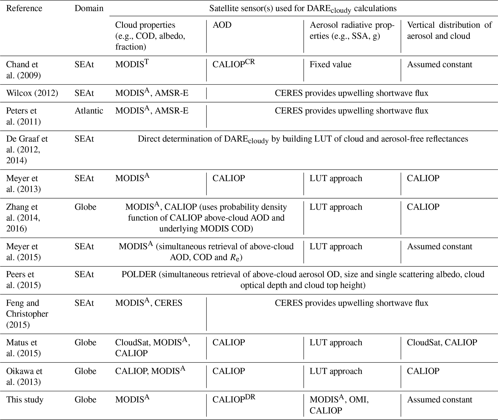
Table 2 lists some passive (i.e., Spinning Enhanced Visible and InfraRed Imager, SEVIRI; Moderate Resolution Imaging Spectroradiometer, MODIS; Polarization and Directionality of Earth's Reflectances, POLDER; Ozone Monitoring Instrument, OMI; or the Scanning Imaging Absorption Spectrometer for Atmospheric Chartography, SCIAMACHY) and active (i.e., CALIOP and CloudSat) satellite sensors that were used to detect and quantify the AAC AODs. Among the peer-reviewed studies of Table 2, those few that present DARE_cloudy results (see Table 1) are denoted by a “+” sign in the first column.

Table 2 Studies that observe AAC using passive and active satellite sensors (i.e., from left to right, SEVIRI, POLDER, CloudSat, OMI, MODIS, SCIAMACHY, CALIOP; see Appendix C for acronyms). When using CALIOP, the authors either use the standard Level 2 products (Std), the Depolarization method (DR) (Hu et al., 2007b) or the color ratio method (CR) (Chand et al., 2008). SEAt stands for southeast Atlantic, SEAs for SE Asia, NEAs for NE Asia and TAt for tropical Atlantic.

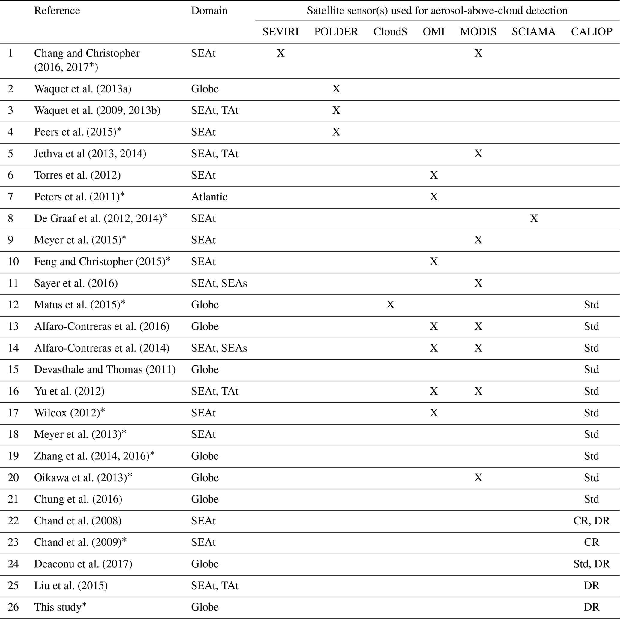
The ^* sign in the first column denotes the presence of DARE_cloudy calculations.

The brightening of clear patches near clouds (Wen et al., 2007) (i.e., “3-D cloud radiative effect” or “cloud adjacency effect”) can introduce biases into the current passive satellite AAC retrieval techniques (i.e., lines 1–11 of Table 2). To minimize these biases, this study relies primarily on CALIOP observations (Winker et al., 2009). CALIOP is a three-channel elastic backscatter lidar with a narrow field of view and a narrow source of illuminating radiation, which limits cloud adjacency effects and the subsequent cloud contamination of aerosol data products (Zhang et al., 2005; Wen et al., 2007; Várnai and Marshak, 2009). CALIOP measures high-resolution (1∕3 km in the horizontal and 30 m in the vertical in low and middle troposphere) profiles of the attenuated backscatter from aerosols and clouds at visible (532 nm) and near-infrared (1064 nm) wavelengths along with polarized backscatter in the visible channel (Hunt et al., 2009). These data are distributed as part of the Level 1 CALIOP products. The Level 2 products are derived from the Level 1 products using a succession of sophisticated retrieval algorithms (Winker et al., 2009). The Level 2 processing is composed of a feature detection scheme (Vaughan et al., 2009), a module that classifies features according to layer type (i.e., cloud versus aerosol) (Liu et al., 2010) and subtype (i.e., aerosol species) (Omar et al., 2009), and, finally, an extinction retrieval algorithm (Young and Vaughan, 2009) that retrieves profiles of aerosol backscatter and extinction coefficients and the total column AOD based on modeled values of the extinction-to-backscatter ratio (also called lidar ratio and represented by the symbol S_a) inferred for each detected aerosol layer subtype.

A few studies use standard CALIOP Level 2 aerosol and cloud layer products to determine AAC occurrence across the globe (see lines 12–21 in Table 2). However, a study by Kacenelenbogen et al. (2014) demonstrates that the standard version 3 CALIOP aerosol products substantially underreport the occurrence frequency of AAC when aerosol optical depths are less than ∼0.02, mostly because these tenuous aerosol layers have attenuated backscatter coefficients less than the CALIOP detection threshold. CALIOP's standard extinction (and optical depth) data products are only retrieved between the tops and bases of detected features, and these boundaries may significantly underestimate the full vertical extent of the layer (Kim et al., 2017; Thorsen et al., 2017; Toth et al., 2018). Furthermore, the Kacenelenbogen et al. (2014) study found essentially no correlation between AAC AOD results reported by the CALIOP and collocated NASA Langley airborne high spectral resolution lidar (HSRL). A subsequent study by Liu et al. (2015) shows that the CALIOP Level 2 standard aerosol data products underestimate dust AAC AOD by ∼26 % over the tropical Atlantic and smoke AAC AOD by ∼39 % over the southeast Atlantic.

For these reasons, a few studies in Table 2 (see lines 22–26) use alternate methods on Level 1 CALIOP products, such as the color ratio (CR) (Chand et al., 2008) or the depolarization ratio (DR) (Hu et al., 2007b; Liu et al., 2015) methods, instead of using the AOD reported in the CALIOP standard Level 2 products.

In this study, we use the DR method and a combination of CALIOP Level 1 and Level 2 data products to compute global estimates of the AAC frequency of occurrence (i.e., f_AAC) and the AAC AOD (i.e., ${\mathit{\tau }}_{\text{AAC}}^{\text{DR}}$) (Sect. 2.1). We then use CALIOP results of f_AAC, ${\mathit{\tau }}_{\text{AAC}}^{\text{DR}}$ and other A-Train satellite products to compute global DARE_cloudy (Sect. 2.2). Section 3 describes the geographical and seasonal distribution of global f_AAC (Sect. 3.1), ${\mathit{\tau }}_{\text{AAC}}^{\text{DR}}$ (Sect. 3.2) and DARE_cloudy results (Sect. 3.3). Section 4 revisits some of the limitations in the method and proposes ways to improve on these DARE_cloudy calculations.

2 Method

2.1 AAC optical depth

Because the CALIOP backscatter signal is totally attenuated below the lowest “feature” detected within any profile (Vaughan et al., 2009), this lowest feature is defined as being opaque. Approximately 69 % of the time, the opaque feature detected in a profile is the Earth's surface (Guzman et al., 2017). In the remainder of the cases, the opaque feature is either a water cloud, an ice cloud or, very rarely, an aerosol layer.

The DR method, which is also known as the “constrained opaque water cloud method” (Liu et al, 2015), relies on opaque water clouds (OWCs) as reflectivity targets. The OWCs in this study are selected using the five criteria listed in Table B2. Most importantly, (1) only one cloud can be detected within a 5 km (15 shot) along-track average (which means, for example, that marine stratus below thin cirrus are excluded), and (2) this one cloud must be opaque (i.e., lowest feature detected in a column, and not subsequently classified as a surface return). Furthermore, all OWCs must be (3) spatially uniform (i.e., detected at single-shot resolution within every laser pulse included in the 5 km averaging interval), (4) assigned a high-confidence score by the CALIOP cloud–aerosol discrimination (CAD) algorithm and (5) identified as a high-confidence water cloud by the CALIOP cloud phase identification algorithm. When there is aerosol above OWCs, the lidar backscatter signal received from the underlying water cloud is reduced in direct proportion to the two-way transmittance of the aerosol layer above. However, because the DR retrieval technique requires backscatter measurements from opaque water clouds (Hu et al., 2007b), it cannot be used to retrieve AOD from aerosols lying above the low, transparent water clouds that are frequently observed over remote oceans, especially in the Southern Hemisphere (e.g., Leahy et al., 2012; Mace and Protat, 2018; O et al., 2018).

Based on Hu et al. (2007a, b), Eq. (2) describes how we compute ${\mathit{\tau }}_{\text{AAC}}^{\text{DR}}$ using the DR method above OWCs.

$$\begin{array}{}\text{(2)}& {\mathit{\tau }}_{\text{AAC}}^{\text{DR}}=-\mathrm{0.5}\times \ln \left[{\text{IAB}}_{\text{SS,AAC}}^{\text{OWC}}/{\text{IAB}}_{\text{SS,CAC}}^{\text{OWC}}\right]\end{array}$$

Here IAB${}_{\text{SS,AAC}}^{\text{OWC}}$ is the single scattering value (subscript SS) of the layer-integrated attenuated backscatter (IAB) for an OWC underlying one or more aerosol layer(s) above the cloud. IAB${}_{\text{SS,CAC}}^{\text{OWC}}$ is the single scattering value of the IAB for an OWC underlying clear air above clouds (CAC). By CAC, we mean that there are no aerosols detected above the OWC. In this study, we consider ${\mathit{\tau }}_{\text{AAC}}^{\text{DR}}$ valid when positive. According to Eq. (2), this means that IAB${}_{\text{SS,AAC}}^{\text{OWC}}$ needs to always be smaller in magnitude than IAB${}_{\text{SS,CAC}}^{\text{OWC}}$ and ${\mathit{\tau }}_{\text{AAC}}^{\text{DR}}$ equals zero when IAB${}_{\text{SS,AAC}}^{\text{OWC}}$ equals IAB${}_{\text{SS,CAC}}^{\text{OWC}}$.

Appendix B provides additional information about the application of Eq. (2) and the various steps needed to derive ${\mathit{\tau }}_{\text{AAC}}^{\text{DR}}$. We list the selection criteria used to identify the OWC dataset in this study and describe the corrections required to obtain single-scattering estimates of IAB from measurements that contain substantial contributions from multiple scattering (Appendix B1). We also describe the technique used for distinguishing between CAC and AAC conditions (Appendix B2) and illustrate our derivation of an empirical parameterization of IAB${}_{\text{SS,CAC}}^{\text{OWC}}$ as a global function of latitude and longitude (Appendix B3).

As reported in Table 2, the CALIOP DR method was used to study the African dust transport pathway over the tropical Atlantic (Liu et al., 2015) and the African smoke transport pathway over the southeast Atlantic (Liu et al., 2015; Chand et al., 2008, 2009). More recently, the CALIOP DR method was also used by Deaconu et al. (2017) to assess POLDER AAC AOD values (Waquet et al., 2009, 2013b; Peers et al., 2015) across the globe. In this study, we extend the previous regional studies of Liu et al. (2015) and Chand et al. (2008, 2009) to derive global CALIOP-based AAC AOD estimates. Let us note that, in our study, the accuracy of ${\mathit{\tau }}_{\text{AAC}}^{\text{DR}}$ depends on measurements of targets of very high signal-to-noise ratio (SNR) such as OWCs in clear skies and OWCs underlying aerosol layers.

2.2 AAC direct aerosol radiative effects

Having first retrieved global values of ${\mathit{\tau }}_{\text{AAC}}^{\text{DR}}$ from the CALIOP measurements, we then compute global estimates of DARE_cloudy using DISORT (DIScrete ORdinate Radiative Transfer; Stamnes et al., 1988; Buras et al., 2011), a six-stream plane-parallel radiative transfer model with molecular absorption characterized by a correlated-k distribution scheme (Fu and Liou, 1992) that is embedded within the LibRadtran Radiative Transfer (RT) package (Emde et al., 2016). Hereafter, our seasonally and spatially gridded ($\mathrm{4}{}^{\circ }\times \mathrm{5}{}^{\circ }$) averaged SW (250 to 5600 nm) global TOA DARE_cloudy results will be called DARE_OWC, as they pertain to a specific category of clouds (i.e., OWCs) defined according to the CALIOP data selection criteria set forth in Table B2. We list the following input parameters to DISORT in order to derive estimates of DARE_OWC:

1. Atmospheric profiles of pressure, temperature, air density, ozone, water vapor, CO₂ and NO₂ use standard US atmosphere profiles (Anderson et al., 1986).

2. Aerosol intensive radiative properties (i.e., properties that depend solely on aerosol species and are unrelated to the aerosol amount) are informed by seasonal maps ($\mathrm{4}{}^{\circ }\times \mathrm{5}{}^{\circ }$, daytime in 2007) of combined MODIS–OMI–CALIOP (MOC) retrieved median spectral extinction coefficients, single scattering albedos and asymmetry parameters at 30 different wavelengths. As an example, Fig. A1 in the Appendix shows the seasonal maps of MOC SSA at 546.3 nm that were used in the calculation of DARE_OWC. These MOC retrievals, described in Appendix A, are the basis of a companion study (Redemann et al., 2019). Let us note that we only use the shape of the MOC extinction coefficient spectrum and not its actual magnitude; the MOC spectral extinction coefficient spectra is normalized to the seasonal 2008–2012 average value of either ${\mathit{\tau }}_{\text{AAC}}^{\text{DR}}$ or ${\mathit{\tau }}_{\text{AAC}}^{\text{DR}}\times f_{\text{AAC}}$ within each grid cell. Our method assumes similar aerosol radiative properties above clouds and in nearby clear-sky regions.

3. Aerosol extensive radiative properties (i.e., properties that depend on the aerosol amount present in the atmosphere) are informed by seasonal maps ($\mathrm{4}{}^{\circ }\times \mathrm{5}{}^{\circ }$, nighttime from 2008 to 2012) of either CALIOP ${\mathit{\tau }}_{\text{AAC}}^{\text{DR}}$ (see Eq. 2) or CALIOP ${\mathit{\tau }}_{\text{AAC}}^{\text{DR}}\times f_{\text{AAC}}$. We chose to use nighttime CALIOP ${\mathit{\tau }}_{\text{AAC}}^{\text{DR}}$ or ${\mathit{\tau }}_{\text{AAC}}^{\text{DR}}\times f_{\text{AAC}}$ results in the estimation of DARE_OWC because, at nighttime, the CALIOP SNR is not affected by ambient solar background and leads to a more accurate measurement of the aerosol signal (compared to daytime). By doing this, we implicitly chose a better accuracy in the aerosol extensive radiative properties over a temporal overlap between aerosol extensive (nighttime) and intensive (daytime) radiative properties.

4. Cloud albedos are computed from cloud droplet effective radius (R_e) and cloud optical depth (COD) information inferred from MODIS averaged monthly $\mathrm{1}{}^{\circ }\times \mathrm{1}{}^{\circ }$ grids (i.e., liquid water cloud products of MYD08_M3: “Cloud Effective Radius Liquid Mean Mean” and “Cloud Optical Thickness Liquid Mean Mean”, Platnick 2015) from 2008 to 2012 (see Eqs. 1–9 of Peng et al., 2002). These maps are then further gridded (to $\mathrm{4}{}^{\circ }\times \mathrm{5}{}^{\circ }$) and seasonally averaged to match the format of the aerosol radiative properties. Figure A2 shows the seasonal maps of MODIS COD that were used in the calculation of DARE_OWC.

5. Aerosol and cloud layer heights are assumed constant across the globe (between 3–4 and 2–3 km respectively in this study), similar to other studies in Table 1 (e.g., Meyer et al., 2015).

6. Earth's surface albedo uses global gap-filled Terra and Aqua combined MODIS BRDF–albedo products. It uses the 16-day closest product (i.e., MCD43GF) to the middle of each season (i.e., 15 January for DJF, 15 April for MAM, 15 July for JJA and 15 October for SON). In the open ocean, the Cox and Munk (1954) sea surface albedo parameterization is applied with a wind speed of 10 m s⁻¹.

Using these inputs, Daily DARE_OWC results for each of the $\mathrm{4}{}^{\circ }\times \mathrm{5}{}^{\circ }$ grid cells are obtained by averaging 24 LibRadtran RT calculations, corresponding to 24 different sun positions at each hour of the day.

3 Results

3.1 AAC occurrence frequencies

To provide the necessary context for interpreting our TOA radiative transfer calculations, we first establish the observational AAC occurrence frequencies from which we will subsequently compute estimates of DARE_OWC. Figure 1 illustrates the annual gridded mean (5 years) global occurrence frequencies of single-layer clouds (panel a), opaque water clouds that are suitable for the DR method (panel b) and aerosol-above-clouds cases using the DR method (panel c). Figure 1d shows the difference between the number of AAC cases using the DR method (i.e., number of cases with ${\mathit{\tau }}_{\text{AAC}}^{\text{DR}}>\mathrm{0}$) and the number of AAC cases using the standard Version 3 CALIOP product.

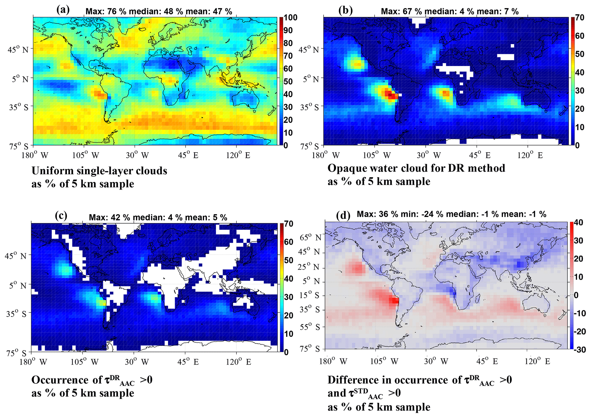
Figure 1 During nighttime, from 2008 to 2012 on a $\mathrm{4}{}^{\circ }\times \mathrm{5}{}^{\circ }$ grid: occurrence frequencies of (a) uniform single-layer clouds (C1–C3 of Table B2), (b) opaque water clouds suitable for the DR method (C1–C5 of Table B2; these clouds can be obstructed or unobstructed) and (c) AAC cases that show a positive ${\mathit{\tau }}_{\text{AAC}}^{\text{DR}}$ at 532 nm. Panel (d) shows the difference between the number of AAC cases using the DR method (i.e., number of cases with ${\mathit{\tau }}_{\text{AAC}}^{\text{DR}}>\mathrm{0}$) and the number of AAC cases using the standard Version 3 CALIOP product (i.e., number of cases with ${\mathit{\tau }}_{\text{AAC}}^{\text{STD}}>\mathrm{0}$); CALIOP AAC cases using the standard algorithm are defined as 5 km columns showing an uppermost layer classified as aerosols and a cloud layer anywhere below that aerosol layer; the cloud itself does not have to satisfy any of the criteria of Table B2. Grid cells are $\mathrm{4}{}^{\circ }\times \mathrm{5}{}^{\circ }$ latitude–longitude. The percentages in (a)–(d) use the number of 5 km CALIOP samples within each grid cell as a reference. White pixels show either no CALIOP observations, no CALIOP OWC detection, a small number of CALIOP unobstructed OWCs or a small number of positive ${\mathit{\tau }}_{\text{AAC}}^{\text{DR}}$ values. The title of each map shows the global maximum, median and mean values.

Uniform single-layer clouds (i.e., C1–C3 of Table B2) are detected in ∼47 % of all 5 km CALIOP samples across the globe (see Fig. 1a). In other words, at any one time, approximately half of the globe is covered by uniform single-layer clouds. As expected, the highest occurrence of those clouds is in the high- and low-latitude bands and especially over the southern oceans. According to Fig. 1b, OWCs suitable for the DR method (i.e., C1–C5 of Table B2) are mostly in the marine stratocumulus regions and represent a mean of 7 % of all 5 km CALIOP samples across the globe. This significant reduction from half-the-globe coverage is explained by the five criteria used to select OWCs for the application of the DR method (i.e., C1–C5 of Table B2). The highest occurrence of OWCs can be found offshore from the west coasts of North and South America, southwest Africa and Australia. In particular, OWC cover ranges from 60 % to 75 % over the region of the southeast Atlantic in August (Klein and Hartmann, 1993). Also, the southeastern Pacific region off the Peruvian and Chilean coasts is the location of the largest and most persistent stratocumulus deck in the world (Klein and Hartmann, 1993). The percentage of AAC cases (i.e., AAC cases showing positive ${\mathit{\tau }}_{\text{AAC}}^{\text{DR}}$) at the basis of our study is very small compared to the total number of 5 km CALIOP profiles per grid cell (i.e., mean of 5 % in Fig. 1c). This is primarily due to a small number of low OWC used for the DR method across the globe (when comparing Fig. 1a and b).

Figure 1d illustrates the difference in occurrence frequencies of AAC cases using the DR method compared to the standard Version 3 CALIOP product. Negative values, shown in blue, indicate the fraction of cases for which the DR method fails to detect above-cloud aerosols that are reported in the standard CALIOP product. Similarly, positive values, shown in red, indicate the number of cases for which above-cloud aerosols are detected by the DR method but not reported in the standard CALIOP data product. Unlike the AAC cases detected using the DR method, the AAC cases obtained from the CALIOP standard product do not impose any restrictions on the nature of the underlying clouds. Instead, the CALIOP standard product reports aerosol detected above both opaque and transparent clouds, irrespective of cloud thermodynamic phase. The blue regions in Fig. 1d show that, relative to the CALIOP standard product, our implementation of the DR method could be failing to detect AAC cases over most of the land surfaces and over the Arabian Sea, the tropical Atlantic and the southeast Atlantic regions. The lack of AAC cases offshore from the southwest coast of Africa in the DR method dataset is the result of our conservative data filtering strategy. Because the IABs of aerosol-contaminated OWCs can differ significantly from those measured in pristine, aerosol-free conditions, OWCs suspected of being aerosol-contaminated (which are ubiquitous in this part of the world and very common over continents) are specifically excluded from our DR method analyses (see Appendix B3 for more details). However, some regions such as the NE and SE Pacific exhibit up to 40 % more AAC cases when using the DR method. The SE Pacific region, especially offshore from Chile, shows particularly tenuous aerosols, with attenuated backscatter values that typically fall below the CALIOP detection limit, thus hampering the detection of AAC using the standard CALIOP algorithm (Kacenelenbogen et al., 2014).

In the rest of this study, the frequency of occurrence of AAC, f_AAC, is defined as follows:

$$\begin{array}{}\text{(3)}& {\displaystyle }{f}_{\text{AAC}}=N_{\text{AAC}}/N_{\text{OWC}},\end{array}$$

where N_AAC is the number of AAC cases (i.e., cases showing a positive ${\mathit{\tau }}_{\text{AAC}}^{\text{DR}}$ at 532 nm) and N_OWC is the number of OWCs within each $\mathrm{4}{}^{\circ }\times \mathrm{5}{}^{\circ }$ grid cell. Let us note that different studies use different references when computing the frequency of occurrence of AAC. The definition in Eq. (3) is similar to the one in Zhang et al. (2016) (see their Eq. 1) and different from Devasthale and Thomas (2011), where f_AAC is defined as the ratio of AAC cases to the total number of CALIOP observations (similar to what is shown in Fig. 1c).

Figure 2 illustrates the global seasonal f_AAC (see Eq. 3) from 2008 to 2012. We find a median global f_AAC of 58 % to 61 % with regional values that can reach more than 80 % in some regions such as the southeast Atlantic, especially during the JJA season. The AAC occurrence frequencies in Fig. 2 generally agree with previous findings (Zhang et al., 2016; Devasthale and Thomas, 2011) on the location and season of highest f_AAC.

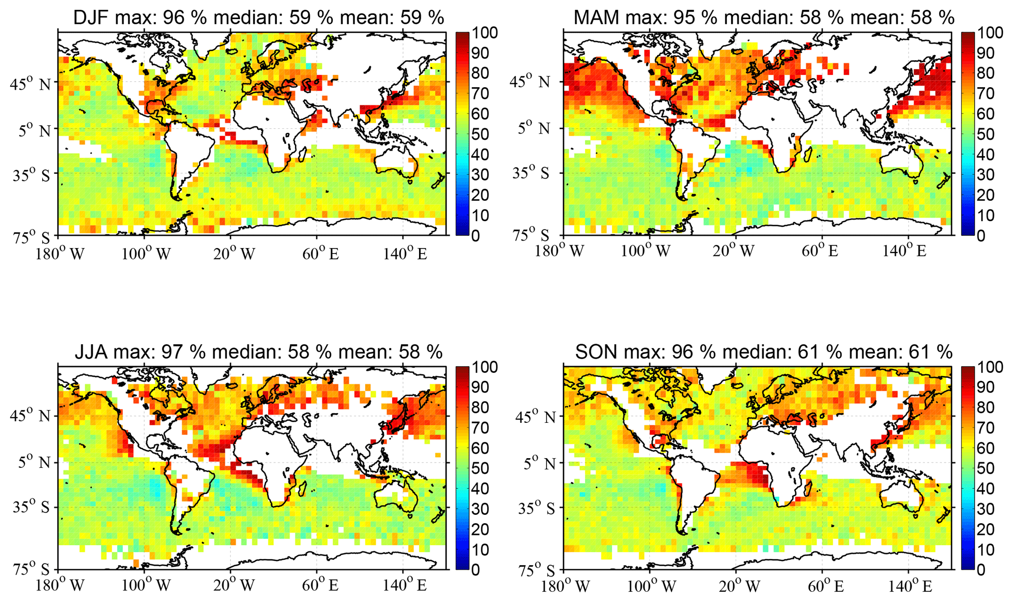
Figure 2 Global seasonal $\mathrm{4}{}^{\circ }\times \mathrm{5}{}^{\circ }$ nighttime AAC occurrence frequency (noted f_AAC; see Eq. 3) from 2008 to 2012. White pixels show either no CALIOP observations, a limited number of CALIOP unobstructed OWCs or a limited number of positive ${\mathit{\tau }}_{\text{AAC}}^{\text{DR}}$ values. White pixels are not considered in the global mean and median f_AAC values in the title of each map. The title of each map shows the global maximum, median and mean values.

3.2 AAC optical depths

Figure 3 introduces the global, nighttime and multiyear (2008–2012) AAC optical depths (${\mathit{\tau }}_{\text{AAC}}^{\text{DR}}$; see Eq. 2) dataset that was computed in this study.

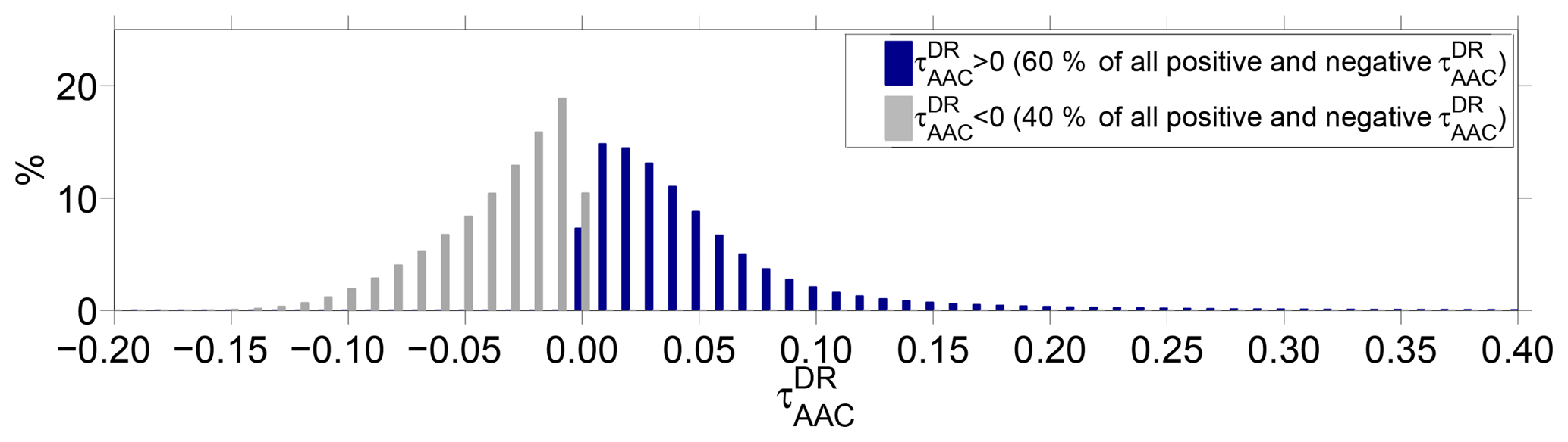
Figure 3 Global distribution of ${\mathit{\tau }}_{\text{AAC}}^{\text{DR}}$ at 532 nm. Positive (i.e., valid) ${\mathit{\tau }}_{\text{AAC}}^{\text{DR}}$ values are in dark blue (N∼3.4 million) and negative ${\mathit{\tau }}_{\text{AAC}}^{\text{DR}}$ values in grey (N∼2.2 million). These are nighttime CALIOP measurements from 2008 to 2012.

About 40 % (i.e., 2.2 million data points) of the initial dataset (i.e., N∼5.6 million) shows negative ${\mathit{\tau }}_{\text{AAC}}^{\text{DR}}$ values and were flagged as invalid data (see grey values in Fig. 3). When looking at all valid (i.e., positive) ${\mathit{\tau }}_{\text{AAC}}^{\text{DR}}$ values (blue), we show a majority of very small ${\mathit{\tau }}_{\text{AAC}}^{\text{DR}}$ values in the 0.01–0.02 AOD range. This agrees with the findings of Devasthale and Thomas (2011). Let us note that averaging all data points per $\mathrm{4}{}^{\circ }\times \mathrm{5}{}^{\circ }$ grid cell (instead of the native resolution shown in Fig. 3) increases the AOD bin of maximum AAC occurrence globally from 0.01 (Fig. 3) to 0.03.

Table 3 shows four different ways of computing global seasonal and annual averages of aerosol optical depth above clouds: we use either ${\mathit{\tau }}_{\text{AAC}}^{\text{DR}}$ or ${\mathit{\tau }}_{\text{AAC}}^{\text{DR}}\times f_{\text{AAC}}$ (see Case I–II or III–IV) and then either (i) exclude all cases of ${\mathit{\tau }}_{\text{AAC}}^{\text{DR}}<\mathrm{0}$ from the average (i.e., as in Case I and Case III), or (ii) set all cases of ${\mathit{\tau }}_{\text{AAC}}^{\text{DR}}<\mathrm{0}$ to zero, and include these samples in the averages (i.e., as in Case II and IV). Let us note that using ${\mathit{\tau }}_{\text{AAC}}^{\text{DR}}\times f_{\text{AAC}}$ (instead of ${\mathit{\tau }}_{\text{AAC}}^{\text{DR}}$) acknowledges the fact that some OWCs present no overlying aerosols. In this case, we assume that when the DR technique retrieves an invalid AAC measurement, f_AAC=0 and there are no aerosols above the cloud.

Table 3 Global seasonal and annual averages of ${\mathit{\tau }}_{\text{AAC}}^{\text{DR}}$ (Case I and II) or ${\mathit{\tau }}_{\text{AAC}}^{\text{DR}}\times f_{\text{AAC}}$ (Case III and IV) when assuming either (i) ${\mathit{\tau }}_{\text{AAC}}^{\text{DR}}<\mathrm{0}$ cases are excluded from the averages (Case I and III) or (ii) ${\mathit{\tau }}_{\text{AAC}}^{\text{DR}}<\mathrm{0}$ cases are set to zero and included in the averages (Case II and IV). Annual averages here (last column) are the mean of the seasonal averages.

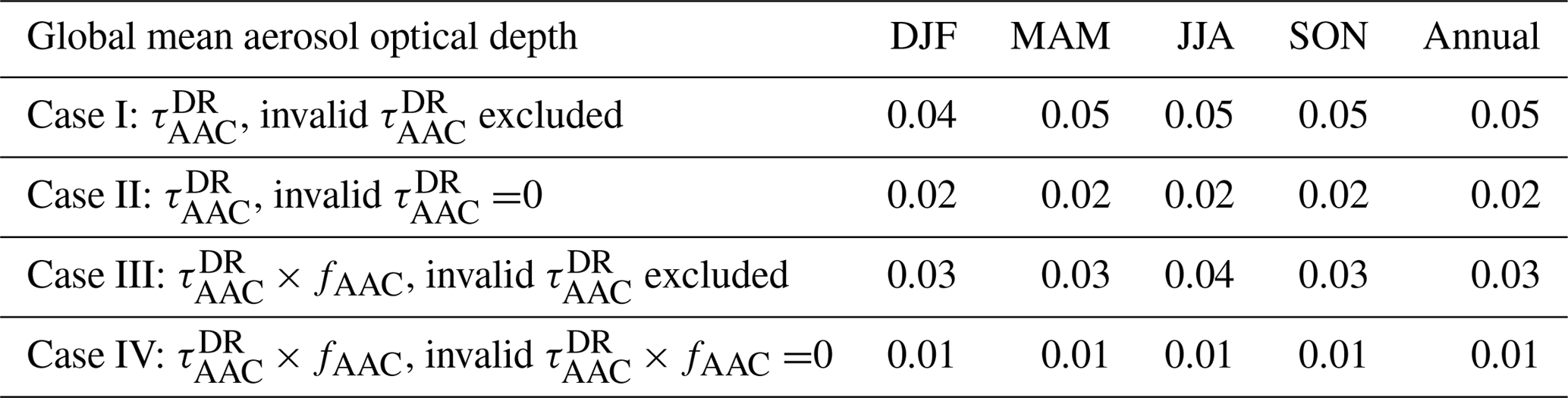
Figure 4 shows global seasonal nighttime median ${\mathit{\tau }}_{\text{AAC}}^{\text{DR}}\times f_{\text{AAC}}$ from 2008 to 2012 (i.e., as in Case III of Table 3). The title of each seasonal map (DJF, MAM, JJA, SON respectively) in Fig. 4 shows the global maximum (0.11, 0.13, 0.22, 0.20 respectively), median (0.02 for all seasons) and mean (0.03 in DJF, MAM and SON and 0.04 in JJA) ${\mathit{\tau }}_{\text{AAC}}^{\text{DR}}\times f_{\text{AAC}}$ values.

We do not expect the ${\mathit{\tau }}_{\text{AAC}}^{\text{DR}}\times f_{\text{AAC}}$ values of Fig. 4 to be similar to the results of Zhang et al. (2014), Devasthale and Thomas (2011), Alfaro-Contreras et al. (2016) or Yu and Zhang (2013) (see Table 2) as these studies use standard CALIOP Level 2 aerosol and cloud layer products for AAC observations, instead of using the DR method. On the other hand, the results of Fig. 4 seem to be in qualitative agreement with the global AAC AOD derived from spaceborne POLDER observations (Waquet et al., 2013a). Let us note that Waquet et al. (2013a) have to assume an underlying COD larger than 3 to ensure the saturation of the polarized light scattered by the cloud layer. Although Deaconu et al. (2017) make different assumptions in the application of the DR method on CALIOP measurements (e.g., they impose a constant cloud lidar ratio for OWCs with clear air above), they find that POLDER and CALIOP ${\mathit{\tau }}_{\text{AAC}}^{\text{DR}}$ are in good agreement over the southeast Atlantic (R²=0.83) and over the tropical Atlantic (R²=0.82) from May to October 2008.

3.3 AAC direct aerosol radiative effects

3.3.1 Global results of DARE_OWC

Figure 5 shows the seasonal TOA SW DARE_OWC estimates (W m⁻²) that use CALIOP ${\mathit{\tau }}_{\text{AAC}}^{\text{DR}}\times f_{\text{AAC}}$ (see Fig. 4) as input to a radiative transfer model, together with the other parameters described in Sect. 2.2. DARE_OWC in Fig. 5 is set equal to zero (i.e., white pixels) if DARE_OWC is invalid or missing.

Figure 4 Global seasonal $\mathrm{4}{}^{\circ }\times \mathrm{5}{}^{\circ }$ nighttime median ${\mathit{\tau }}_{\text{AAC}}^{\text{DR}}\times f_{\text{AAC}}$ from 2008 to 2012. Underlying clouds satisfy the criteria in Table B2. White pixels show either no CALIOP observations, a limited number of CALIOP unobstructed OWCs or a limited number of positive ${\mathit{\tau }}_{\text{AAC}}^{\text{DR}}$ values. White pixels are not included when calculating the global mean and median ${\mathit{\tau }}_{\text{AAC}}^{\text{DR}}$ values in the title of each map (i.e., as in Case III in Table 3). Note that if the white pixels were set equal to zero, the seasonal and annual global ${\mathit{\tau }}_{\text{AAC}}^{\text{DR}}$ values would correspond to Case IV in Table 3. The title of each map shows the global maximum, median and mean values.

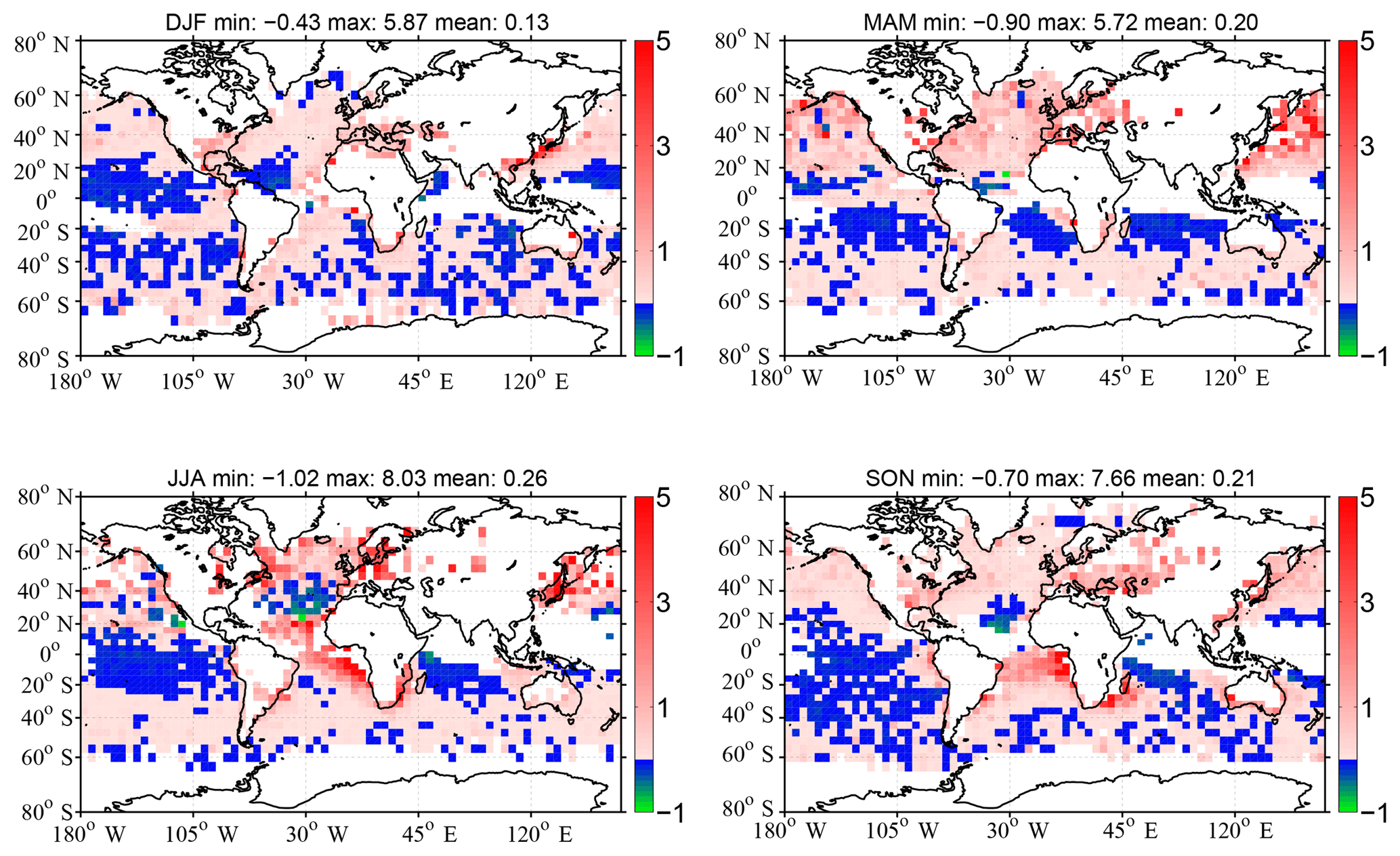
Figure 5 Global seasonal $\mathrm{4}{}^{\circ }\times \mathrm{5}{}^{\circ }$ TOA SW DARE_OWC estimates (W m⁻², as described in Sect. 2.2). A white pixel is counted as DARE_OWC=0 in the global mean DARE_OWC values in the title of each map. White pixels show a limited number of CALIOP OWCs, positive ${\mathit{\tau }}_{\text{AAC}}^{\text{DR}}$ values or auxiliary MODIS–OMI–CALIOP combined satellite observations. The title of each map shows the global minimum, maximum and mean values.

Similar to TOA DARE_cloudy values from combined A-Train satellites in Oikawa et al. (2013) (see their Fig. 10) and from general circulation models (GCMs) (e.g., SPRINTARS) in Shulz et al. (2006) (see their Figs. 6 and 7), TOA DARE_OWC values in Fig. 5 are mostly positive (i.e., a warming effect due to less energy leaving the climate system) across the globe. We find, globally, 72 % positive $\mathrm{4}{}^{\circ }\times \mathrm{5}{}^{\circ }$ DARE_OWC values (i.e., N=4045) against 28 % negative values (i.e., N=1581) when considering all four seasons in Fig. 5. On the other hand, the highest negative TOA DARE_OWC values in Fig. 5 (i.e., cooling effects shown in green pixels) are over the tropical Atlantic (in MAM, JJA and SON), in the Pacific Ocean offshore from Mexico (in JJA) and at the periphery of the Arabian Sea (in JJA).

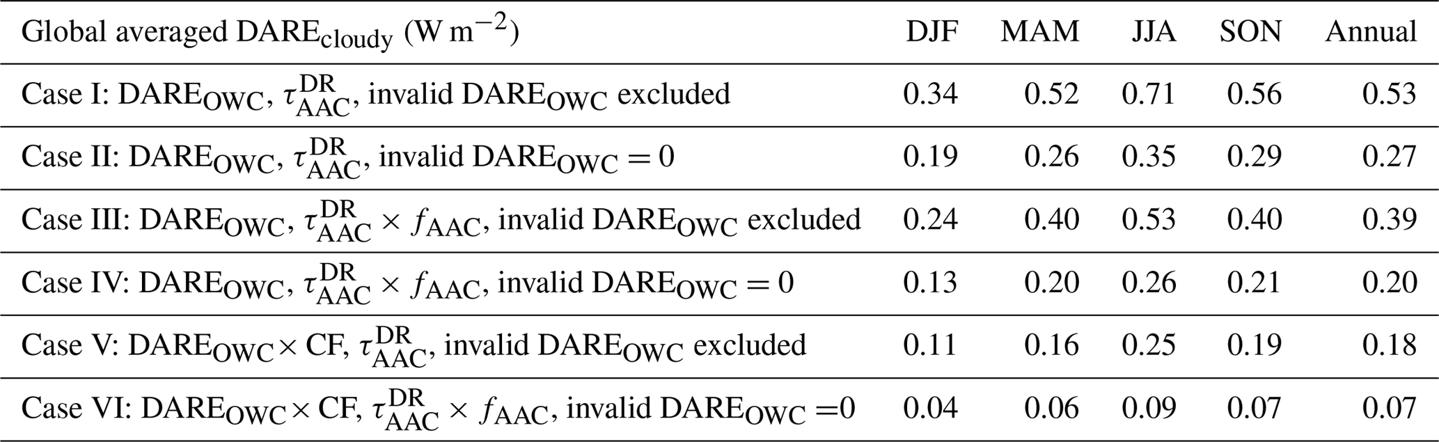
There are multiple ways to compute the global seasonal and annual DARE_cloudy averages (i.e., DARE_OWC in our case), and it is not clear which method would bring us closer to the true DARE_cloudy state of the planet. For this reason, we list several different methods in Table 4. We either use CALIOP ${\mathit{\tau }}_{\text{AAC}}^{\text{DR}}$ or CALIOP ${\mathit{\tau }}_{\text{AAC}}^{\text{DR}}\times f_{\text{AAC}}$ (Case I–II or III–IV) and we either exclude invalid DARE_OWC values or set invalid DARE_OWC=0 (Case I–III or II–IV). For completeness and as an intermediate step towards DARE_all-sky (see Eq. 1), Case V and VI show the global seasonal averages of DARE_OWC× cloud fraction (CF), instead of DARE_OWC. The CF values use monthly MODIS AQUA MYD08_M3 products (variable “Cloud_Retrieval_Fraction_Liquid_FMean”), which are seasonally averaged and gridded to $\mathrm{4}{}^{\circ }\times \mathrm{5}{}^{\circ }$.

Table 4 Global seasonal and annual averages of TOA SW DARE_OWC estimates (W m⁻², as described in Sect. 2.2). Annual averages (last column) are the mean of the seasonal averages (e.g., 0.53 for Case I is the average of 0.34, 0.52, 0.71 and 0.56); CF stands for cloud fraction.

Global seasonal and annual DARE_OWC averages (see titles in Fig. 5 and Table 4) in our study represent the surface area of each grid cell. Each valid DARE_OWC value per pixel on each map of Fig. 5 is multiplied by the surface of the pixel. These values per grid cell are then summed up and divided by the sum of the surface of all valid grid cells.

Figure 5 corresponds to the setting of Case IV in Table 4. The reason why we have decided to showcase this setting is because it closely resembles the settings of the DARE_cloudy calculations in Zhang et al. (2016); i.e., it assumes DARE = 0 when CALIOP cannot detect an aerosol layer. Figure 5 shows positive global seasonal DARE_OWC averages between 0.13 and 0.26 W m⁻² (and an annual average of 0.20 W m⁻² in Table 4) as well as the lowest DARE_OWC values when compared to DARE_OWC values from Case I through Case IV in Table 4. These values are nonetheless much larger than the global annual ocean DARE_cloudy values reported in Zhang et al. (2016) and Schulz et al. (2006) (e.g., annual average of 0.015 W m⁻² reported over ocean in Zhang et al., 2016). Moreover, Matus et al. (2015) find (see their Table 2) a global TOA DARE_cloudy value of 0.1 W m⁻² over thick clouds (these clouds are similar to our study), compensated by a global TOA DARE_cloudy value of −2 W m⁻² over thin clouds.

Section 3.3.2 further analyzes DARE_OWC, together with f_AAC, ${\mathit{\tau }}_{\text{AAC}}^{\text{DR}}$, SSA and COD results in a few selected regions and compares these results to previous studies.

3.3.2 Regional results of DARE_OWC

The f_AAC results in Fig. 2 help us define six major AAC “hotspots” over the northeast Pacific (NEPa), southeast Pacific (SEPa), tropical Atlantic (TAt), southeast Atlantic (SEAt), Indian ocean, offshore from western Australia (InWA) and northwest Pacific (NWPa). To assist in the analysis of the remaining figures in this study, Figure 6 and Table 5 briefly describe these six AAC hotspots.

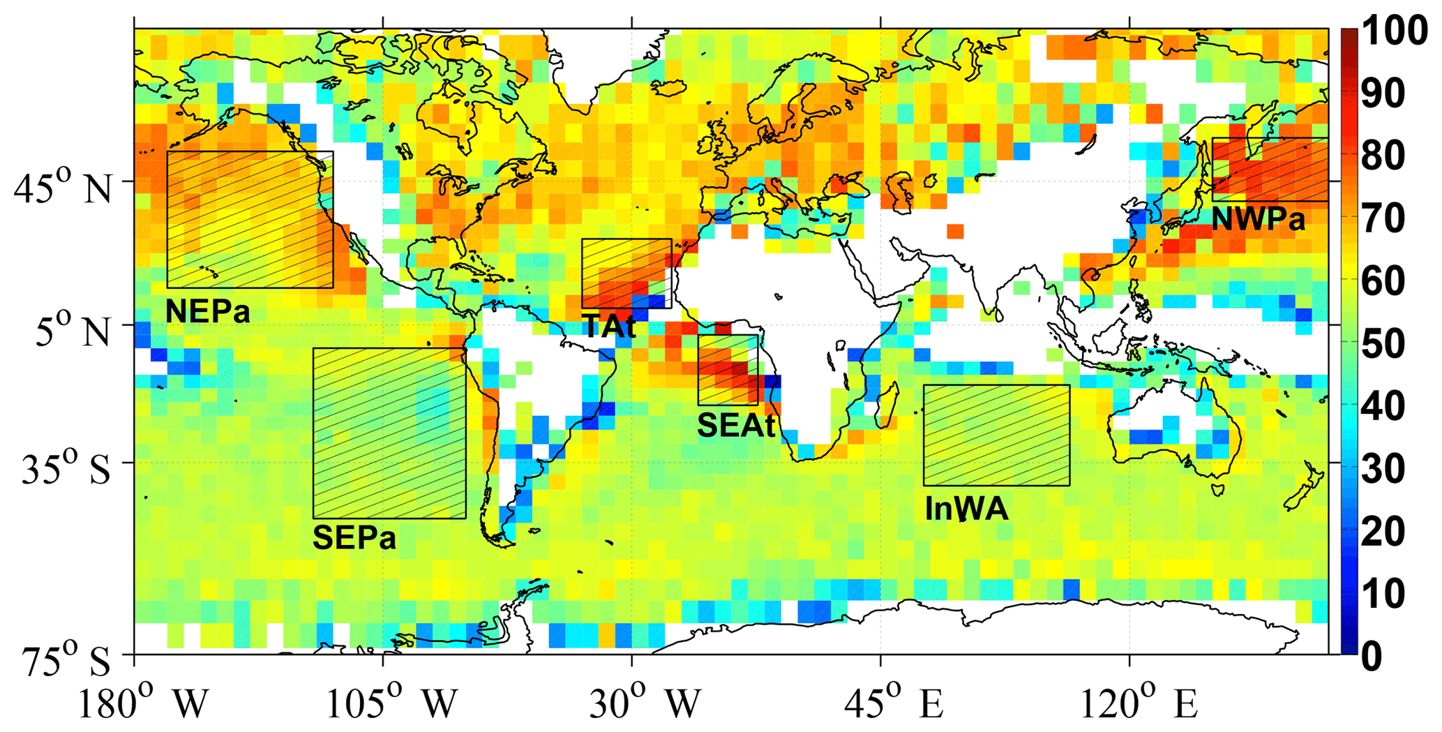
Figure 6 Six regions of high AAC occurrence, further defined in Table 5. Background map is the global annual $\mathrm{4}{}^{\circ }\times \mathrm{5}{}^{\circ }$ nighttime AAC occurrence frequency (f_AAC; see Eq. (3) and Fig. 2 for seasonal f_AAC maps). Global annual maximum, median and mean f_AAC values are respectively 93 %, 57 % and 57 %.

Table 5 Six regions of high AAC occurrence (see Fig. 6), their season of highest AAC occurrence and its corresponding mean f_AAC value.

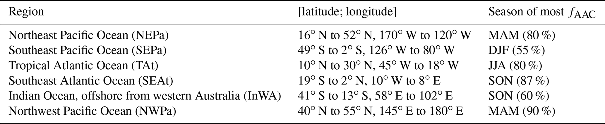
Figure 7a illustrates the mean regional, seasonal or annual estimates of SW TOA DARE_OWC (W m⁻²) in each region of Table 5. Figure 7b–f show the primary parameters used in the DARE_OWC calculations (see Sect. 2.2): the mean regional, seasonal or annual (panel b) percentage of grid cells that show valid (i.e., positive) $f_{\text{AAC}}\times {\mathit{\tau }}_{\text{AAC}}^{\text{DR}}$ values compared to the total number of $\mathrm{4}{}^{\circ }\times \mathrm{5}{}^{\circ }$ pixels in each region; (panel c) CALIOP f_AAC values; (panel d) CALIOP $f_{\text{AAC}}\times {\mathit{\tau }}_{\text{AAC}}^{\text{DR}}$ values; (panel e) assumed overlying SSA values at 546.3 nm; and (panel f) assumed underlying COD values from MODIS.

Figure 7 Mean regional, seasonal or annual (a) estimated SW TOA DARE_OWC (W m⁻², calculation is described in Sect. 2.2), (b) percentage of grid cells that show valid $f_{\text{AAC}}\times {\mathit{\tau }}_{\text{AAC}}^{\text{DR}}$ (i.e., positive) values compared to the total number of $\mathrm{4}{}^{\circ }\times \mathrm{5}{}^{\circ }$ pixels in each region, (c) CALIOP f_AAC (%), (d) $f_{\text{AAC}}\times {\mathit{\tau }}_{\text{AAC}}^{\text{DR}}$ (no unit), (e) assumed overlying SSA at 546.3 nm from a combination of MODIS–OMI–CALIOP and (f) assumed underlying COD from MODIS in each region of Table 5. DARE_OWC in (a) is computed using the Case IV of Table 4.

Table 6 reports the estimated seasonal or annual regional minimum, maximum, mean and standard deviations of our TOA DARE_OWC dataset (i.e., values of Fig. 7a).

Table 6 Estimated SW TOA DARE_OWC (W m⁻², setting is Case IV of Table 4) in each region of Table 5.

We record positive TOA DARE_OWC values above 1 W m⁻² in Fig. 7a over TAt in JJA (1.08±1.66), SEAt in JJA and SON (2.49±2.54 and 2.87±2.33), and NWPa in MAM (1.98±1.85). Let us note that the highest positive TOA DARE_OWC values in Fig. 7a and in Table 6 may not be entirely representative of each region, because they are based on a smaller number of valid DARE_OWC results (86 % valid values in JJA in TAt, 58 %–88 % in JJA–SON in SEAt and 69 % in MAM in NWPa). SEAt and NWPa are the only regions showing an all-positive range of DARE_OWC values in Table 6 (i.e., within 0.20 and 7.59 and within 0.07 and 5.72 W m⁻² respectively). The spread (i.e., standard deviation) of those mean regional DARE_OWC is of the same order of magnitude as the mean values themselves. For example, although TAt shows an annual mean DARE_OWC value of 0.41 W m⁻², most points (i.e., about 68 %, assuming a normal distribution of DARE_OWC) are within 0.41±0.74 W m⁻² (see Table 6). Those regions and seasons of highly positive DARE_OWC values are associated with the highest CALIOP ${\mathit{\tau }}_{\text{AAC}}^{\text{DR}}\times f_{\text{AAC}}$ values (see Fig. 7d: 0.12 in JJA in TAt, 0.12–0.13 in JJA–SON in SEAt and 0.10 in MAM in NWPa). They are also associated with lower SSA values (i.e., <0.94 in Fig. 7e), typical of more light-absorbing aerosols such as biomass burning. The underlying COD values are fairly constant (between ∼5 and 10 in Fig. 7f), except for a noticeably higher COD over the NWPa region (between ∼15 and 25 in Fig. 7f). NWPa is the region of highest latitudes in our study (i.e., between 40 and 55^∘ N). More variation in the COD at higher latitudes is also observed in Fig. A2 in the Appendix. This agrees with King et al. (2013), who show a larger zonal variation of COD (and increased uncertainty in the MODIS cloud property retrievals) in the higher latitudes of both hemispheres, particularly in winter (see their Fig. 12b).

When computing mean DARE_OWC results within the “southeast Atlantic” region defined in Zhang et al. (2016) (i.e., 30^∘ S to 10^∘ N; 20^∘ W to 20^∘ E instead of 19^∘ S to 2^∘ N; 10^∘ W to 8^∘ E in our study), we find a small fraction of valid pixels (i.e., an average of ∼37 %) but a mean annual DARE_OWC value of 0.57 W m⁻², which resides within their range of annual DARE_cloudy values (i.e., 0.1–0.68 W m⁻² in Zhang et al., 2016). Similar to Matus et al. (2015), the season of highest DARE_OWC is SON over the southeast Atlantic (they find 10 % of DARE_OWC larger than 10 W m⁻² over thick clouds with COD > 1; see their Fig. 9d). However, our DARE_OWC results are significantly higher than the ones in Zhang et al. (2016) in our SEAt region (defined as a smaller region and offshore from the “southeast Atlantic” region in Zhang et al., 2016) as well as in the TAt (similar latitude–longitude boundaries to the ones of region “TNE Atlantic” in Zhang et al., 2016) and the NWPa (similar boundaries to “NW Pacific” in Zhang et al., 2016) regions.

We emphasize that the DARE_OWC estimates in this study are not directly comparable to many previous studies (see Table 1) because of different spatial domain, period, satellite sensors and associated uncertainties. This will lead to the detection of different fractions of AAC above different types of clouds and different AAC types across the globe. The calculations of DARE_cloudy can also differ greatly depending on different AAC aerosol radiative properties assumptions above clouds (especially absorption) and different assumptions in aerosol and cloud vertical heights (see Table 1).

Apart from the major differences in methods and sensors, it seems reasonable to say that we are missing AAC cases over pure dust-dominant regions such as the Arabian Sea or the TAt region (compared to Zhang et al., 2016, and Matus et al., 2015, for example). Both Matus et al. (2015) and Zhang et al. (2016) use the CALIOP Level 2 standard products to distinguish among a few aerosol types and infer specific aerosol optical properties in their DARE_cloudy. According to Fig. 1d, SEAt, TAt and the Arabian Sea are regions where we might be missing up to 40 % of AAC cases when using the DR technique compared to the CALIOP standard products. The number of potentially missing AAC cases in our study is larger over the Arabian sea (0–30^∘ N and 40–80^∘ E due to the limited number of OWCs suitable for the DR method (see Appendix B1). Zhang et al. (2016) show that pure dust aerosols over these dust-dominant regions tend to produce a negative DARE_cloudy when the underlying COD is below ∼7 and this is the case for most of the clouds over these regions in their study. In summary, two factors in the DR method seem to hamper the detection of AAC in these regions: the low cloud optical depths of underlying clouds and very few cases of “clear air” above clouds. As a consequence, we propose that the positive DARE_OWC values in our study should, in reality, be counter-balanced by more negative dust-driven DARE_cloudy values over regions such as TAt and the Arabian Sea. On the other hand, the DARE_cloudy results from Matus et al. (2015) and Zhang et al. (2016) might also differ from the true global DARE_cloudy state of the planet for different reasons. As described in Matus et al. (2015), using CALIOP Level 2 standard products as in Matus et al. (2015) and Zhang et al. (2016) could lead to possible misclassification of dust aerosols as clouds (Omar et al., 2009), specifically around cloud edges in the TAt region. Moreover, even if the AAC is correctly detected in Matus et al. (2015) and Zhang et al. (2016), the amount of AAC AOD might be biased low due to their use of the CALIOP Level 2 standard products (Kacenelenbogen et al., 2014).

4 Uncertainties in our DARE above-cloud results and the path forward

4.1 Detecting and quantifying the true amount of AAC cases

Our study mainly uses CALIOP Level 1 measurements to detect aerosols above specific OWCs that satisfy the criteria given in Table B2. We suggest that the number of CALIOP profiles that contain aerosols over any type of cloud (instead of only OWCs in this study) should be informed by a combination of different techniques applied to CALIOP observations (e.g., the standard products, the DR and the CR technique). Airborne observations such as those from the ObseRvations of Aerosols above Clouds and their intEractionS (ORACLES) field campaigns (Zuidema et al., 2016) are well suited for providing further guidance on when to apply which technique.

To the best of our knowledge, the true global occurrence of aerosols above any type of cloud remains unknown. This question cannot be entirely answered with the use of CALIOP observations only. We suggest that a more complete global quantification and characterization of aerosol above any type of cloud should be informed by a combination of AAC retrievals from CALIOP, passive satellite sensors (e.g., POLDER (Waquet et al., 2013a, b; Peers et al., 2015; Deaconu et al., 2017), MODIS (Meyer et al., 2013; Zhang et al., 2014, 2016; see Table 2) and model simulations (Schulz et al., 2006).

4.2 Considering the diurnal variability of aerosol and cloud properties

While we consider the diurnal cycle of solar zenith angles in our DARE_cloudy calculations, we use MODIS for underlying COD and cloud R_e information as well as a combination of MODIS, OMI and CALIOP for overlying aerosol properties (see Sect. 2.2). By using A-Train satellite observations (i.e., the AQUA, AURA and CALIPSO platforms), with an overpass time of 13:30 local time at the Equator, we are only using a daily snapshot of cloud and aerosol properties and not considering their daily variability.

Min and Zhang (2014) show a strong diurnal cycle of cloud fraction over the SEAt region (i.e., a 5-year mean trend of diurnal cloud fraction using SEVIRI that varies from ∼60 % in the late afternoon to 80 % in the early morning on their Fig. 4). According to Min and Zhang (2014) (see their Table 2), assuming a constant cloud fraction derived from MODIS/AQUA generally leads to an underestimation (less positive) by ∼16 % in the DARE_all-sky calculations (see Eq. 1). Further studies should explore the implications of diurnal variations of COD and cloud R_e on DARE_cloudy results using, for example, geostationary observations from SEVIRI.

Daily variations of aerosol (intensive and extensive) radiative properties above clouds cannot be ignored either. Arola et al. (2013) and Kassaniov et al. (2013) both show that even when the AOD varies strongly during the day, the accurate prediction of 24 h average DARE_non-cloudy requires only daily averaged properties. However, in the case of under-sampled aerosol properties, such as when using A-Train derived aerosol properties (this study), the error in the 24 h DARE_non-cloudy can be as large as 100 % (Kassaniov et al., 2013). Xu et al. (2016) show that the daily mean TOA DARE_non-cloudy is overestimated by up to 3.9 W m⁻² in the summertime in Beijing if they use a constant MODIS AQUA AOD value, compared to accounting for the observed hourly-averaged daily variability. Kassaniov et al. (2013) propose that using a simple combination of MODIS TERRA and AQUA products would offer a reasonable assessment of the daily averaged aerosol properties for an improved estimation of 24 h DARE_non-cloudy.

4.3 Considering the spatial and temporal variability of cloud and aerosol fields

We have used coarse-resolution (i.e., $\mathrm{4}{}^{\circ }\times \mathrm{5}{}^{\circ }$) seasonally gridded aerosol and cloud properties in our DARE_OWC calculations (see Sect. 2.2). As a consequence, subgrid-scale variability (or heterogeneity) of cloud and aerosol properties has not been considered. This approach is similar to assuming spatially and temporally homogeneous cloud and aerosol fields in our DARE_OWC results.

Marine boundary layer (MBL) clouds show significant small-scale horizontal variability (Di Girolamo et al., 2010; Zhang et al., 2011). Using mean gridded COD in DARE_cloudy calculations, for example, can lead to significant biases in DARE_cloudy calculations, an effect called the “plane-parallel albedo bias” (e.g., Oreopoulos et al., 2007; Di Girolamo et al., 2010; Zhang et al., 2011, 2012). Min and Zhang (2014) show that using a mean gridded COD significantly overestimates (by ∼10 % over the SEAt region) the DARE_cloudy results when the cloud has significant subgrid horizontal heterogeneity. Furthermore, this overestimation increases with increasing AOD, COD and cloud inhomogeneity. Future studies should examine the difference between DARE_cloudy results calculated with gridded mean COD and cloud R_e values (this study) and DARE_cloudy results calculated with MODIS Level 3 joint histograms of MODIS COD and cloud R_e (e.g., similar to Min and Zhang, 2014).

Aerosol spatial variation can be significant over relatively short distances of 10 to 100 km, depending on the type of environment (Anderson et al., 2003; Kovacs, 2006; Santese et al., 2007; Shinozuka and Redemann, 2011; Schutgens et al., 2013). Shinozuka and Redemann (2011) argue that only a few environments can be more heterogeneous than the Canadian phase of the ARCTAS (Arctic Research of the Composition of the Troposphere from Aircraft and Satellites) experiment, where the air mass was subject to fresh local biomass emissions. In this type of environment, they observed a 19 % variability of the AOD over a 20 km length (comparable in scale to a $\sim \mathrm{0.1}{}^{\circ }\times \mathrm{0.1}{}^{\circ }$ area). They also found a 2 % variability in the AOD over the same length in a contrasting homogeneous environment that occurred after a long-range aerosol transport event. As a consequence, similar to using a mean gridded underlying COD and cloud R_e, using mean gridded overlying aerosol radiative properties could very well bias our DARE_OWC results.

As a preliminary investigation into the sources and magnitudes of these potential biases, we have used TOA DARE_non-cloudy (see Eq. 1) estimates derived using well-collocated aerosol properties (hereafter called “retrieve-then-average” or R-A) from a companion study (Redemann et al., 2019; see Appendix A) and compared those to DARE_non-cloudy estimates computed using seasonally gridded mean aerosol properties at seasonally gridded mean vertical heights (hereafter called “average-then-retrieve” or A-R). Both DARE_non-cloudy results obtained with the two methods are compared over ocean and at a resolution of $\mathrm{4}{}^{\circ }\times \mathrm{5}{}^{\circ }$.

A majority (i.e., ∼58 %) of A-R DARE_non-cloudy results are within ±35 % of the R-A DARE_non-cloudy results. We find very few (i.e., ∼1 %) negative R-A DARE_non-cloudy values paired with positive A-R DARE_non-cloudy values and very few large differences between both methods (i.e., less than 1 % of the differences are above ±10 W m⁻²). However, we find a weak agreement between A-R and R-A DARE_non-cloudy values during each of the seasons (i.e., a correlation coefficient between 0.21 and 0.34). The A-R DARE_non-cloudy values are generally biased high relative to the R-A calculations, as illustrated by positive mean and median values of the A-R to R-A differences (0.64 and 0.92 W m⁻² respectively; standard deviation of 2.25). When computing the global seasonal mean A-R and R-A DARE_non-cloudy values separately, we find that the global seasonal A-R DARE_non-cloudy values overestimate the global seasonal R-A DARE_non-cloudy values by 17 %, 19 %, 21 % and 17 % in DJF, MAM, JJA and SON. Moreover, the seasonal median A-R DARE_non-cloudy values overestimate the seasonal median R-A DARE_non-cloudy values in all six regions of Table 5 (i.e., median differences between 0.28 W m⁻² in NWPa in SON and 3.05 W m⁻² in SEAt in JJA). The geospatial distributions of these differences in DARE calculation strategies are illustrated in Fig. 8.

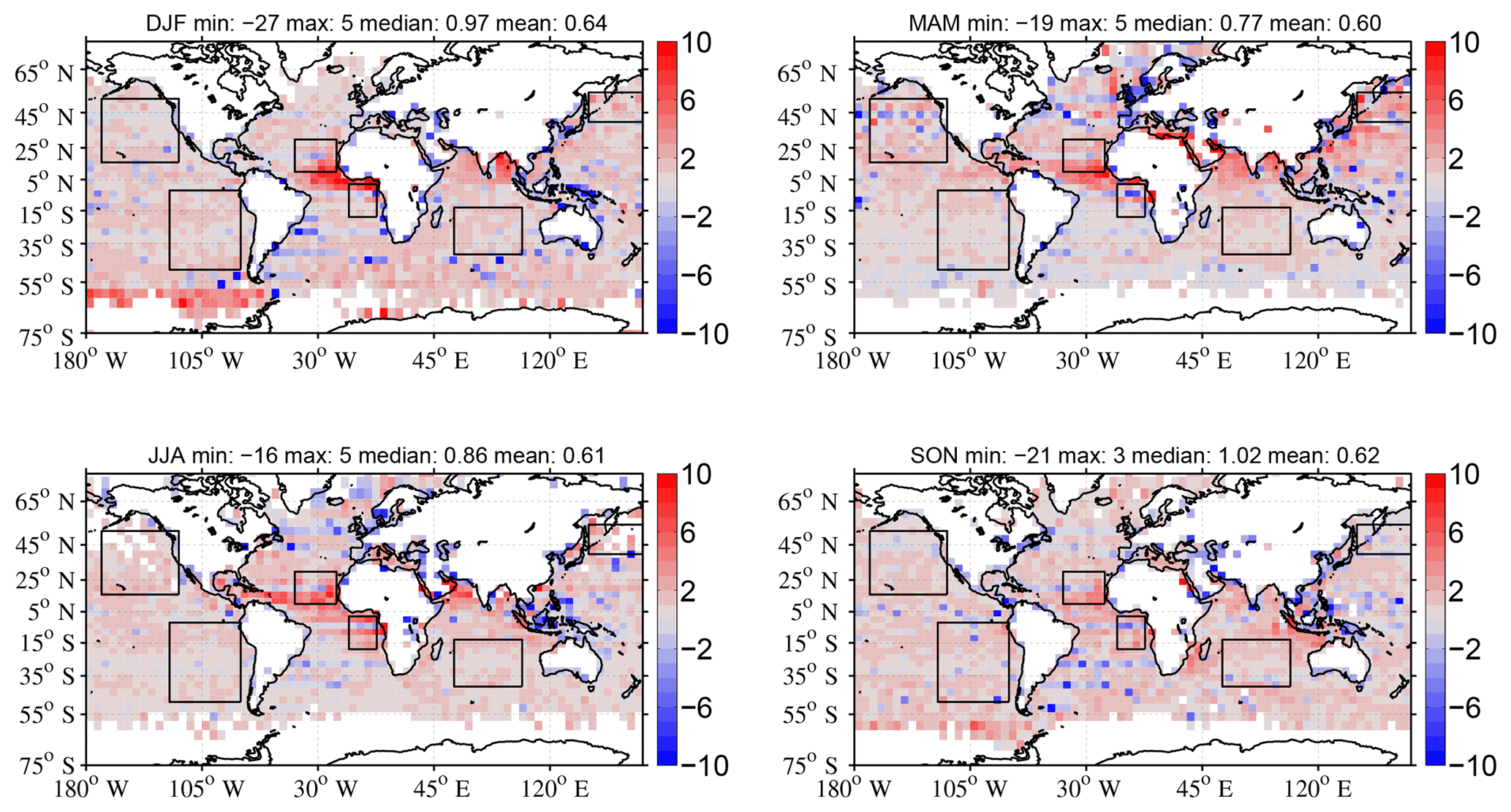
Figure 8 Seasonal maps showing the differences in SW TOA DARE_non-cloudy computed using the average-then-retrieve (A-R) and the retrieve-then-average (R-A) strategies. Positive values (in red) show regions where the A-R DARE calculations are larger, whereas negative values (in blue) show regions where the R-A DARE calculations are larger. The squares show different regions defined in Table 5. The title of each map shows the global minimum, maximum, median and mean values.

4.4 Assuming similar intensive aerosol properties above clouds and in nearby cloud-free skies

In the calculation of DARE_OWC, we assume similar intensive aerosol properties above clouds and in nearby clear skies. This assumption might not be valid and should be investigated in future studies by comparing aerosol properties and their probability distributions over clear and cloudy conditions using observations from the ORACLES field campaign.

4.5 Assuming fixed aerosol and cloud vertical layers

Finally, longwave (LW) radiative forcing is particularly dependent on the vertical distribution of aerosols, especially for light-absorbing aerosols (Chin et al., 2009). This is because the energy these aerosols reradiate depends on the temperature, and hence their altitude. For example, Penner et al. (2003) emphasize the importance of soot and smoke aerosol injection height in LW TOA DARE_all-sky (see Eq. 1) simulations (higher injection heights tend to enhance the negative LW radiative forcing).

Quijano et al. (2000), Chung et al. (2005) and Chin et al. (2009) demonstrate the importance of an aerosol height, in relation to a cloud height (i.e., the aerosols located above, within or below the clouds) in an accurate estimation of SW TOA DARE_all-sky. Chung et al. (2005), for example, show that varying the relative vertical distribution of aerosols and clouds leads to a range of global anthropogenic SW TOA DARE_all-sky from −0.1 to −0.6 W m⁻² (using a combination of MODIS satellite, AERONET ground-based observations and CTM simulations; see their Table 2).

However, here, we concentrate on cases of aerosol layers overlying clouds in order to compute SW TOA DARE_cloudy. Aerosol and cloud layer heights are assumed constant across the globe in our study (see Sect. 2.2). Future studies should incorporate mean gridded (i.e., $\mathrm{4}{}^{\circ }\times \mathrm{5}{}^{\circ }$ in this study) seasonal CALIOP Level 2 aerosol and cloud vertical profiles into the calculation of DARE_OWC.

However, constraining clouds between 2 and 3 km in our study does not seem unreasonable as our AAC AOD calculations using the DR method can only be applied to aerosols overlying specific low opaque water clouds with, among other criteria, an altitude below 3 km (see Table B2). On the other hand, constraining aerosols between 3 and 4 km in our study is not realistic over many parts of the globe (e.g., see Fig. 7 of Devasthale et al., 2011). For example, over the region of the southeast Atlantic during the ORACLES campaign, the HSRL team observed an aerosol layer located on average between 2 and 5 km, and overlying a cloud at an average altitude of 1.2 km.

According to Zarzycki et al. (2010), the underlying cloud properties are orders of magnitude more crucial to the computation of DARE_cloudy than the location of the aerosol layer relative to the cloud, as long as the aerosol is above the cloud. In other words, the forcing does not seem to depend on the height of the aerosols above clouds as much as other parameters such as the AOD, SSA or cloud albedo. Zarzycki et al. (2010) investigated this assumption and found that over low and middle clouds, forcing changed by ∼1 %–3 % through the heights where the Black Carbon burden was the largest. These small changes in forcing are likely products of a change in atmospheric transmission above the aerosol layer (Haywood and Ramaswamy, 1998) (e.g., a change in the aerosol height is linked to a change in the integrated column water vapor above the aerosol layer and this, in turn, would alter the incident solar radiation).

5 Conclusions

We have computed a first approximation of global seasonal TOA shortwave direct aerosol radiative effects (DARE) above opaque water clouds (OWCs), DARE_OWC, using observation-based aerosol and cloud radiative properties from a combination of A-Train satellite sensors and a radiative transfer model. Our DARE_OWC calculations make three major departures from previous peer-reviewed results: (1) they use extensive aerosol properties derived from the depolarization ratio (DR) method applied to Level 1 CALIOP measurements, whereas previous studies often use CALIOP Level 2 standard products which introduce higher uncertainties and known biases; (2) our DARE_OWC calculations are applied globally, while most previous studies focus on specific regions of high AAC occurrence such as the southeast Atlantic; and (3) our calculations use intensive aerosol properties retrieved from a combination of A-Train satellite sensor measurements (e.g., MODIS, OMI and CALIOP).

Our study agrees with previous findings on the locations and seasons of the maximum occurrence of AAC across the globe. We identify six regions of high AAC occurrence (i.e., AAC hotspots): South and North East Pacific (SEAt and NEPa), tropical and southeast Atlantic (TAt and SEAt), Indian Ocean offshore from western Australia (InWA), and northwest Pacific (NWPa). We define ${\mathit{\tau }}_{\text{AAC}}^{\text{DR}}$, the aerosol optical depth (AOD) above OWCs, using the DR method on CALIOP measurements, f_AAC, and the frequency of occurrence of AAC cases. We record a majority of ${\mathit{\tau }}_{\text{AAC}}^{\text{DR}}\times f_{\text{AAC}}$ values at 532 nm in the 0.01–0.02 range and that can exceed 0.2 over a few AAC hotspots.

We find positive averages of global seasonal DARE_OWC between 0.13 and 0.26 W m⁻² and an annual global mean DARE_OWC value of 0.20 W m⁻² (i.e., a warming effect on climate). Regional seasonal DARE_OWC values range from −0.06 W m⁻² in the Indian Ocean, offshore from western Australia (in March–April–May), to 2.87 W m⁻² in the southeast Atlantic (in September–October–November). High positive values are usually paired with high aerosol optical depths (>0.1) and low single scattering albedos (<0.94), representative of biomass burning aerosols, for example.

Although the DARE_OWC estimates in this study are not directly comparable to previous studies because of different spatial domains, periods, satellite sensors, detection methods and/or associated uncertainties, we emphasize that they are notably higher than the ones from Zhang et al. (2016), Matus et al. (2015) and Oikawa et al. (2013). In addition to differences in satellite sensors, AAC detection methods and the assumptions enforced in the calculation of DARE_cloudy, there are several other factors that may contribute to the overall higher DARE_OWC values we report in this study. The most likely contributors are (1) a possible underestimate of the number of dust-dominated AAC cases; (2) our use of the DR method on CALIOP Level 1 data to quantify the AAC AOD; and, in particular, (3) the technique we have chosen for aggregating subgrid aerosol and cloud spatial and temporal variability. We discuss each of these in turn in the following paragraphs.

Two factors seem to be preventing the DR method from recording enough AAC cases in these regions: the low cloud optical depths of underlying clouds and very few cases of “clear air” above clouds. The DR method used in this study is restricted to aerosols above OWCs that satisfy a long list of criteria. The AAC dataset in this study underestimates (i) the total number of CALIOP 5 km profiles that contain AAC over all OWCs (i.e., not just suitable to the DR technique), (ii) the total number of CALIOP 5 km profiles that contain AAC over any type of clouds across the globe and (iii) the true global occurrence of AAC over any type of clouds. To the best of our knowledge, the true amount of AAC in (i), (ii) and (iii) remains unknown. A better characterization of the “unobstructed” OWCs in the application of the DR technique on CALIOP measurements might bring us closer to answering (i). A combination of CALIOP standard, DR and CR techniques together with airborne observations (e.g., from the ORACLES field campaign) might answer (ii). Finally, (iii) cannot be answered with only the use of CALIOP observations. The results in this study should be combined with aerosol-above-cloud retrievals from passive satellite sensors (e.g., POLDER, Waquet et al., 2013a, b; Peers et al., 2015; Deaconu et al., 2017, or MODIS, Meyer et al., 2013; Zhang et al., 2014, 2016) and model simulations (Schulz et al., 2006) to obtain a more complete global quantification and characterization of aerosol above any type of clouds.

Compared to other methods, the DR technique applied to CALIOP measurements retrieves ${\mathit{\tau }}_{\text{AAC}}^{\text{DR}}$ with fewer assumptions and lower uncertainties. Other global DARE_cloudy results (e.g., Matus et al., 2015, and Zhang et al., 2016) use CALIOP standard products to detect the AAC cases, quantify the AAC AOD and define the aerosol type (and specify the aerosol intensive properties). These studies rely on the presence of aerosol in concentrations sufficient to be identified by the CALIOP layer detection scheme, and on the ability of the CALIOP aerosol subtyping algorithm to correctly identify the aerosol type and thus select the correct lidar ratio for the AOD retrieval. While several recent studies have taken various approaches to quantifying the amount of aerosol that is not currently being detected in the CALIOP backscatter signals, their general conclusions are unanimous. The CALIOP standard products underestimate above-cloud aerosol loading and the corresponding AAC AOD (Kacenelenbogen et al., 2014; Kim et al., 2017; Toth et al., 2018; Watson-Parris et al., 2018), and this in turn leads to underestimates of both DARE_non-cloudy and DARE_cloudy (Thorsen and Fu, 2015; Thorsen et al., 2017).

In this study, we have assumed spatially and temporally homogeneous clouds and aerosols in our DARE_OWC calculations. As a preliminary investigation of such effects on our calculations, we have compared DARE calculations derived from well collocated aerosol properties (retrieve-then-average) to DARE calculations using seasonally gridded mean aerosol properties (average-then-retrieve). We have shown that the average-then-compute DARE results generally overestimate the retrieve-then-average results both on a global scale and in each of our selected regions. Further research and analysis are required to determine which of these two computational approaches provides the most accurate estimates of real-world DARE.

Appendix A: Method to obtain aerosol radiative properties in non-cloudy (i.e., clear-sky) conditions using MODIS, OMI and CALIOP and to estimate DARE_non-cloudy

A companion paper, Redemann et al. (2019), develops and refines a method for retrieving full spectral (i.e., at 30 different wavelengths) extinction coefficients, single scattering albedo (SSA) and asymmetry parameters from satellite aerosol products in non-cloudy (i.e., clear-sky) conditions. The method requires collocation of quality-screened satellite data, selection of aerosol models that reproduce the satellite observations within stated uncertainties and forward calculation of aerosol radiative properties based on the selected aerosol models. They use MODIS-Aqua AOD at 550 and 1240 nm, CALIPSO integrated backscattering (IBS) at 532 nm and OMI absorption aerosol optical depth (AAOD) at 388 nm (see Table A1). The aerosol radiative properties resulting from this method are called MOC retrievals (for MODIS–OMI–CALIOP).

Table A1 Datasets currently used for global MODIS–OMI–CALIOP (MOC) retrievals of aerosol radiative properties (Redemann et al., 2019); DT: Dark Target; EDB: Enhanced Deep Blue.

¹ For the values after division by CALIPSO layer depth. ² The weight, w_i, is used to calculate the cost function $X=\left(\mathrm{\Sigma }{w}_i\right((x_i-{\widehat{x}}_i)/\mathit{\delta }{\widehat{x}}_i{)}^{\mathrm{2}}{)}^{\mathrm{1}/\mathrm{2}}$, where x_i denotes the retrieved parameters, ${\widehat{x}}_i$ denotes the observables, and $\mathit{\delta }{\widehat{x}}_i$ denotes the uncertainties in the observables.

The choice of OMI satellite algorithms (see Table A1) reflects their assessment of the representativeness of subsampling OMI data along the CALIPSO track; i.e., they compared the probability distribution function (PDF) of the OMI retrievals along the CALIPSO track to the global PDF and chose the dataset that had the best match between global and along-track PDF for the over-ocean and two over-land datasets, the latter being different in their use of MODIS Dark Target (DT) versus Enhanced Deep Blue (EDB) data as the source of AOD. They collocate the MODIS and OMI products within a 40 km × 40 km box centered at each CALIPSO 5 km profile location after Redemann et al. (2012). For the OMAERUV dataset, they choose the SSA product for the layer height indicated by the collocated CALIOP backscatter profile. Their aerosol models emulate those of the MODIS aerosol over-ocean algorithm (Remer et al., 2005). Like the MODIS algorithm, they define each model with a lognormal size distribution and wavelength-dependent refractive index. They then combine two of these models, weighted by their number concentration, and compute optical properties for the bi-modal lognormal size distribution. Unlike the MODIS algorithm, they allow combinations of two fine-mode or two coarse-mode models. They use 10 different aerosol models, which stem from some of the MODIS over-ocean models (Remer et al., 2005) but include more absorbing models, which was motivated by application of their methodology to the Arctic Research of the Composition of the Troposphere from Aircraft and Satellites (ARCTAS) field campaign data, requiring more aerosol absorption than included in the current MODIS over-ocean aerosol models. They use MOC spectral aerosol radiative properties to then calculate direct aerosol radiative effects (i.e., DARE_non-cloudy; see Eq. 1) through a delta-four stream radiative transfer model with 15 spectral bands from 0.175 to 4.0 µm in SW and 12 longwave (LW) spectral bands between 2850 and 0 cm⁻¹ (Fu and Liou, 1992).

In order to use these MOC parameters (retrieved in clear-skies) in our DARE_OWC calculations, we need to assume similar aerosol intensive properties in clear skies compared to above clouds and we need to spatially and/ or temporally grid these MOC parameters. As discussed in Sect. 2.2, we use seasonally averaged MOC spectral SSA, aerosol asymmetry parameter and extinction retrievals on $\mathrm{4}{}^{\circ }\times \mathrm{5}{}^{\circ }$ grids. Figure A1 illustrates seasonal maps of MOC SSA used in our calculations of DARE_OWC.

The DARE_OWC calculations in our study also require information about the underlying cloud optical properties. As discussed in Sect. 2.2, we use seasonally mean gridded COD from MODIS such as illustrated in Fig. A2.

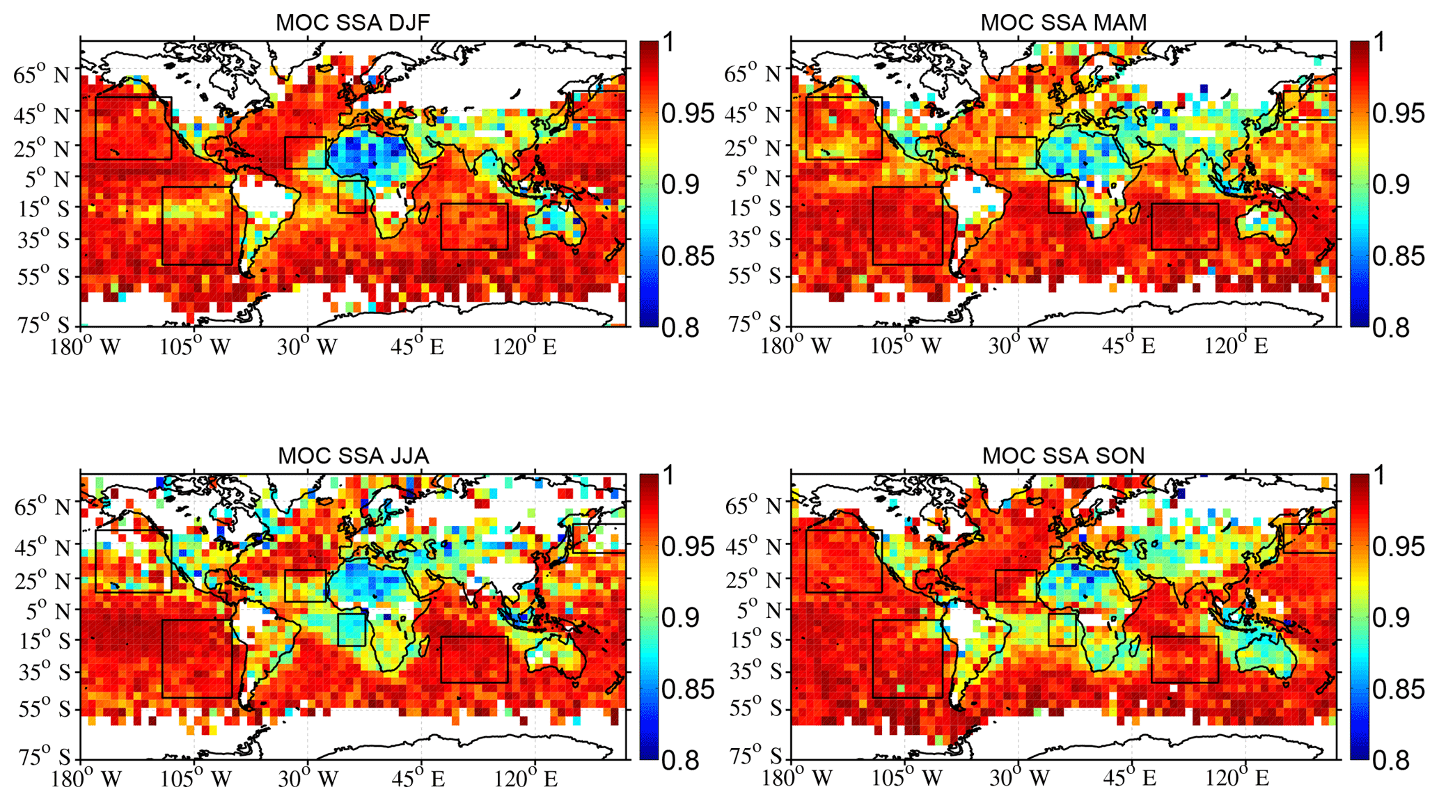
Figure A1 Seasonal maps of MOC SSA at 546.3 nm in 2007 used in the calculations of DARE_OWC. The squares show different regions defined in Table 5.

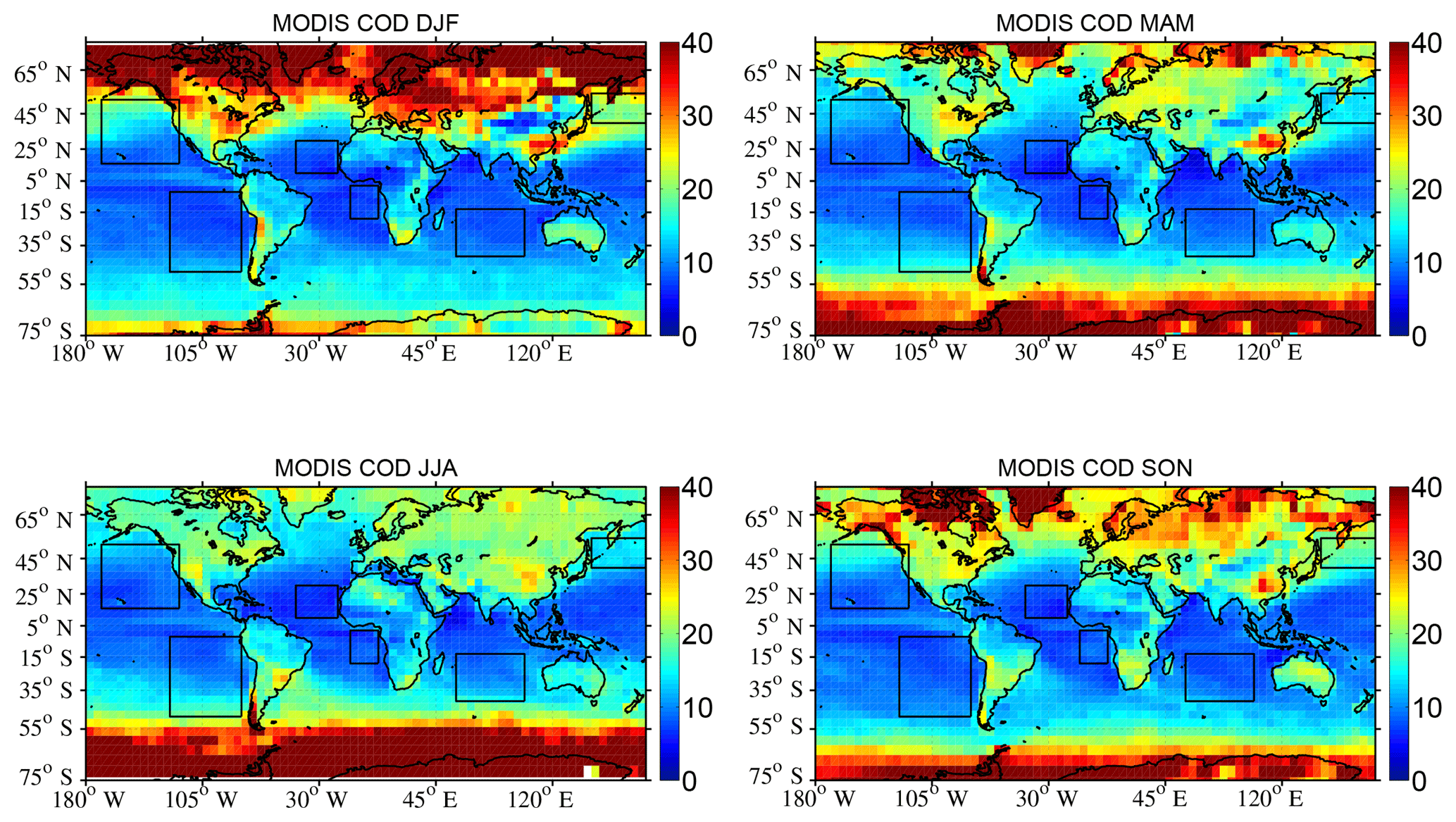
Figure A2 Seasonal maps of COD used in the calculations of DARE_OWC. COD information is inferred from MODIS seasonally averaged monthly $\mathrm{1}{}^{\circ }\times \mathrm{1}{}^{\circ }$ grids (i.e., liquid water cloud products of MYD08_M3: “Cloud Effective Radius Liquid Mean Mean” and “Cloud Optical Thickness Liquid Mean Mean”; Platnick et al., 2015) from 2008 to 2012. The squares show different regions defined in Table 5.

Appendix B: Method for AAC detection and AAC AOD computation

Table B1 Steps required to compute ${\mathit{\tau }}_{\text{AAC}}^{\text{DR}}$.

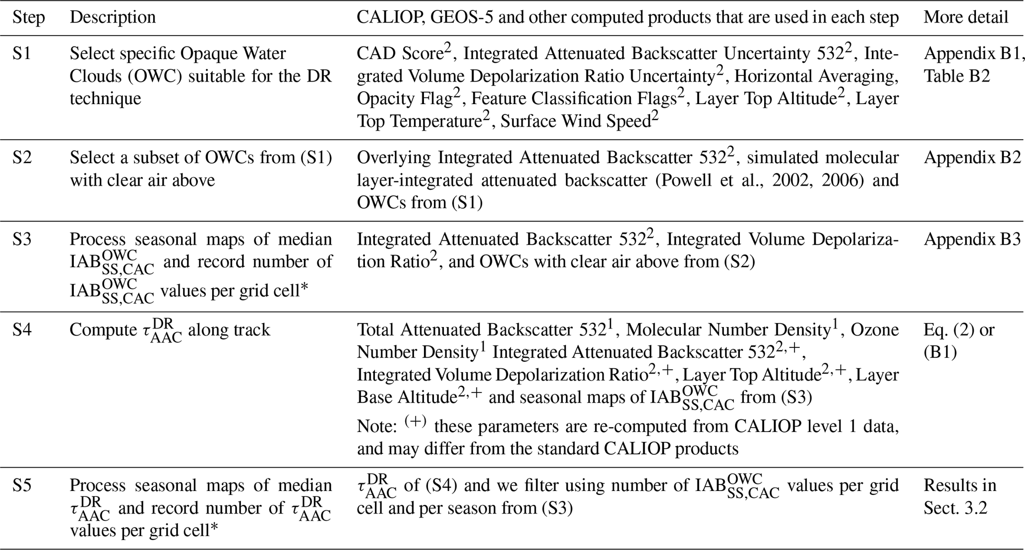
^* We construct global maps of 4×5^∘ pixels using median values. Superscripts 1 and 2 denote respectively CALIOP Level 1 and Level 2 aerosol or cloud layer products.

The depolarization ratio (DR) method (Hu et al., 2007b) used to derive estimates of the optical depths (τ) of aerosols above clouds (AAC) is given in Eq. (2) and repeated here for convenience:

$$\begin{array}{}\text{(B1)}& {\displaystyle }{\mathit{\tau }}_{\text{AAC}}^{\text{DR}}=-\mathrm{0.5}\times \ln \left[{\text{IAB}}_{\text{SS,AAC}}^{\text{OWC}}/{\text{IAB}}_{\text{SS,CAC}}^{\text{OWC}}\right].\end{array}$$

The subscripts SS and CAC represent, respectively, “single scattering” and “clear above clouds”. IAB${}_{\text{SS}}^{\text{OWC}}$ (i.e., either IAB${}_{\text{SS,AAC}}^{\text{OWC}}$ or IAB${}_{\text{SS,CAC}}^{\text{OWC}}$) is the single scattering integrated attenuated backscatter (IAB), derived from the product of the measured 532 nm attenuated backscatter coefficients integrated from cloud top to cloud base, IAB^OWC, and a layer effective multiple scattering factor, η^OWC, derived from the layer-integrated volume depolarization ratio of the water cloud (called δ^OWC) using the following:

$$\begin{array}{}\text{(B2)}& {\displaystyle }{\mathit{\eta }}^{\text{OWC}}={\left[\left(\mathrm{1}-{\mathit{\delta }}^{\text{OWC}}\right)/\left(\mathrm{1}+{\mathit{\delta }}^{\text{OWC}}\right)\right]}^{\mathrm{2}}\end{array}$$

(Hu et al., 2007a). The single scattering IAB is thus derived using the following:

$$\begin{array}{}\text{(B3)}& {\displaystyle }{\text{IAB}}_{\text{SS},X}^{\text{OWC}}={\mathit{\eta }}^{\text{OWC}}\times {\text{IAB}}_{\text{measured},X}^{\text{OWC}}\end{array}$$

for both aerosol above cloud cases (X= AAC) and those cases with clear skies above (X= CAC). An assumption of the DR method is that δ^OWC is negligibly affected by any aerosols that lie in the optical path between the OWC and the lidar.

Table B1 provides a high-level overview of the procedure we use to compute aerosol optical depth (${\mathit{\tau }}_{\text{AAC}}^{\text{DR}}$) above OWCs across the globe. We chose to concentrate on nighttime CALIOP observations only, as they have substantially higher signal-to-noise ratios (SNRs) than the daytime measurements (Hunt et al., 2009).

The first step (S1) is to identify OWCs that are suitable for the application of the DR method. The acceptance criteria used to identify these clouds are described below in Appendix B1 and listed in Table B2. In the second step (S2), we use the overlying integrated attenuated backscatter (i.e., the 532 nm attenuated backscatter coefficients integrated from TOA to the OWC cloud tops) to partition the OWC into two classes: (i) “unobstructed” clouds, for which the magnitude of the overlying IAB suggests that only aerosol-free clear skies lie above and (ii) “obstructed” clouds for which we expect to be able to retrieve positive estimates of ${\mathit{\tau }}_{\text{AAC}}^{\text{DR}}$. Section B2 describes the objective method we have developed to separate unobstructed clouds (for which we can compute IAB${}_{\text{SS,CAC}}^{\text{OWC}}$) from obstructed clouds (for which we calculate IAB${}_{\text{SS,AAC}}^{\text{OWC}})$.

In step (S3), we construct global seasonal maps of median IAB${}_{\text{SS,CAC}}^{\text{OWC}}$ using 5 consecutive years (2008–2012) of CALIOP nighttime data (see Appendix B3). By doing this we can subsequently compute estimates of ${\mathit{\tau }}_{\text{AAC}}^{\text{DR}}$ without invoking assumptions about the lidar ratios of water clouds in clear skies (Hu et al., 2007). Throughout this study, we chose to compute global median values within each grid cell (instead of mean values) to limit the impact of particularly high or low outliers on our statistics.

In step (S4), we compute estimates of ${\mathit{\tau }}_{\text{AAC}}^{\text{DR}}$ for all obstructed OWC within each grid cell using Eq. (2) or (B1) and the 5-year nighttime seasonal median values of IAB${}_{\text{SS,CAC}}^{\text{OWC}}$ from (S3) (i.e., each ${\mathit{\tau }}_{\text{AAC}}^{\text{DR}}$ value along the CALIOP track is computed using one median value of IAB${}_{\text{SS,CAC}}^{\text{OWC}}$ per $\mathrm{4}{}^{\circ }\times \mathrm{5}{}^{\circ }$ pixel and per season).

For the OWCs considered in this study, true layer base cannot be measured by CALIOP, simply because the signal becomes totally attenuated at some point below the layer top. Instead, what is reported in the CALIOP data products is an apparent base, which indicates the point at which the signal was essentially indistinguishable from background levels. Numerous validation studies have established the accuracy of the CALIOP cloud layer detection scheme (e.g., McGill et al., 2007; Kim et al., 2011; Thorsen et al., 2011; Yorks et al., 2011; Candlish et al., 2013). Strong attenuation of the signal by optically thick aerosols above an OWC can, in some cases, introduce biases into the cloud height determination, which would lead to misestimating IAB${}_{\text{SS,AAC}}^{\text{OWC}}$ and subsequent errors in ${\mathit{\tau }}_{\text{AAC}}^{\text{DR}}$. To ensure the use of consistent data processing assumptions throughout our retrievals of ${\mathit{\tau }}_{\text{AAC}}^{\text{DR}}$, we recalculated the components of IAB${}_{\text{SS,AAC}}^{\text{OWC}}$ (i.e., the “Integrated Attenuated Backscatter 532” and “Integrated Volume Depolarization Ratio”) using parameters in the CALIOP Level 1 product (“Total Attenuated Backscatter 532”, “Molecular Number Density” and “Ozone Number_Density”) and optimized estimates of cloud top and base altitudes based on the “Layer Top Altitude” and “Layer Base Altitude” values reported in the CALIOP Level 2 layer product.

Apart from the identification of specific OWCs in step (S1), the primary Level 2 CALIOP parameters used to calculate ${\mathit{\tau }}_{\text{AAC}}^{\text{DR}}$ (S2–S4 in Table B1) are (i) the integrated attenuated backscatter above cloud top to detect “clear air” cases (i.e., “Overlying Integrated Attenuated Backscatter 532” in step S2), (ii) the layer integrated attenuated backscatter of the OWC with clear air above (i.e., “Integrated Attenuated Backscatter 532” in step S3) and (iii) the cloud multiple scattering factor, derived as a function of the layer integrated volume depolarization ratio (i.e., the “Integrated Volume Depolarization Ratio” in S3 and S4).

Below, we list the potential sources of errors associated with those three products:

• a.

  the accuracy of the 532 nm channel calibrations,

• b.

  the SNR of the backscatter data within the layer,

• c.

  the estimation of molecular scattering in the integrated attenuated backscatter (Sect. 3.2.9.1 of the CALIPSO Feature Detection ATBD, http://www-calipso.larc.nasa.gov/resources/pdfs/PC-SCI-202_Part2_rev1x01.pdf, last access: 27 September 2005) and

• d.

  the accuracy of the depolarization calibration (see Sect. 5 in Powell et al., 2009).

Concerning (a), Rogers et al. (2011) show that the NASA LaRC HSRL and CALIOP Version 3 532 nm total attenuated backscatter agree on average within ∼3 %, demonstrating the accuracy of the CALIOP 532 nm calibration algorithms.

Concerning (b), we assume the influence of the SNR returned from the OWC is negligible as the OWCs are strongly scattering features and our dataset is composed of nighttime data only. However, the backscatter from tenuous and spatially diffuse aerosol layers with large extinction-to-backscatter ratios can lie well beneath the CALIOP attenuated backscatter detection threshold. When such layers lie above OWCs, the measured overlying integrated attenuated backscatter can fall within 1 standard deviation of the expected “purely molecular” value that is used to identify CAC (or “unobstructed”) OWC in our dataset (S2; see Appendix B2). Within the context of this study, these tenuous and spatially diffuse aerosol layers can have appreciable AOD, and thus care must be taken to ensure that these sorts of cases are not misclassified as CAC OWC. Appendix B3 discusses such cases, possibly found, for example, over the region of SEAt.

B1 Select specific opaque water clouds suitable for DR technique

Successful application of the DR method (Eq. 2 or B1) requires a very specific type of underlying cloud (step S1 in Table B1). Table B2 lists the criteria we have applied to the CALIOP 5 km cloud layer products for the selection of these specific OWCs across the globe.

Table B2 Criteria used to select the opaque water clouds (OWCs) for the application of the DR method to obtain the AAC frequency of occurrence, AAC optical depth, AAC lidar ratio and DARE_OWC in this study.

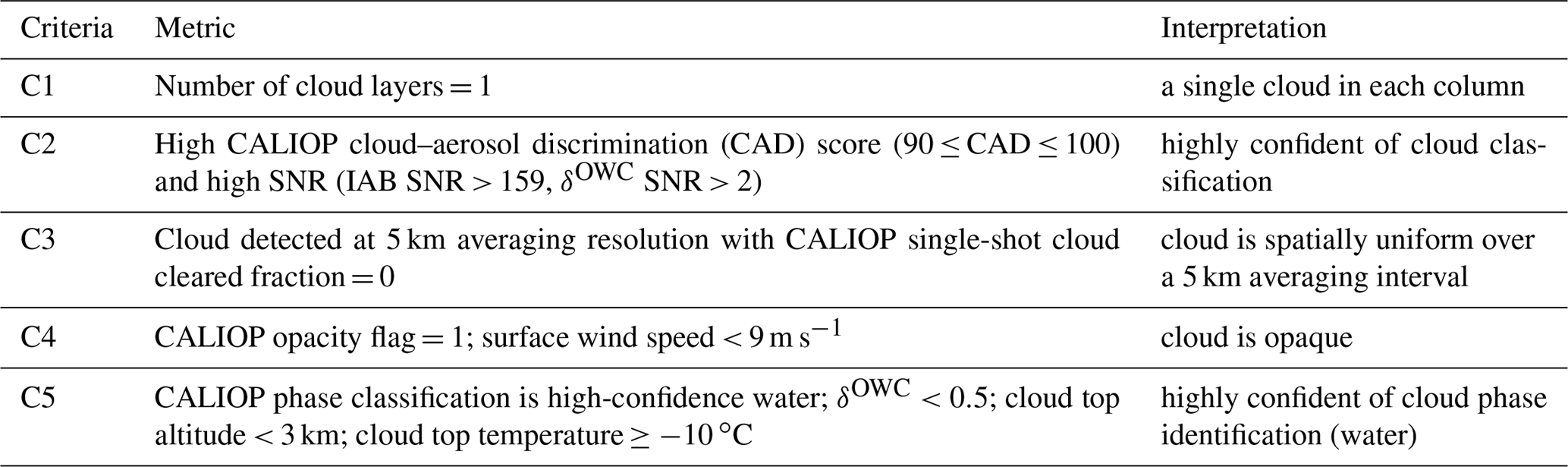
We ensure that each cloud is the only cloud detected within the vertical column (C1) and is guaranteed to be of high quality by imposing filters on various CALIOP quality assurance flags (C2). Imposing the “single-shot cloud cleared fraction = 0” in criterion (C3) ensures that the clouds are uniformly detected at single-shot resolution throughout the full 5 km (15 shot) horizontal extent. As a result, we will intentionally miss any broken clouds and any clouds that show a weaker scattering intensity within one or more laser pulses with the 15 shot average. On the other hand, enforcing the single-shot cloud fraction = 0 criteria simultaneously ensures that all ${\mathit{\tau }}_{\text{AAC}}^{\text{DR}}$ values in this study will lie below a certain threshold: larger values would attenuate the signal to the point that single-shot detection of underlying clouds is no longer likely. Consequently, some highly attenuating biomass burning events (e.g., with ${\mathit{\tau }}_{\text{AAC}}^{\text{DR}}>\mathrm{2.5}$) can be excluded from the cases considered here.

At high surface wind speeds over oceans, the CALIOP V3 layer detection algorithm may fail to detect surface backscatter signals underneath optically thick but not opaque layers. In such cases, CALIOP's standard algorithm may misclassify the column as containing an opaque overlying cloud. To avoid such scenarios, we exclude all the cases with high surface wind conditions (C4). Let us note that this condition was applied on the entire dataset, disregarding the surface type (i.e., land or ocean), as our OWC dataset resides mostly over ocean surfaces (see Fig. 1b).

Criterion (C5) requires that the OWC be both low enough (cloud top below 3km) and warm enough (cloud top temperature above −10 ^∘C as in Zelinka et al., 2012) to ensure that it is composed of liquid water droplets. After applying all the criteria of Table B2, the median OWC top height of our dataset is ∼1.6 km. According to Hu et al. (2009), any feature showing a cloud layer integrated volume depolarization ratio above 50 % should correspond to an ice cloud with randomly oriented particles. Criterion (C5) ensures the deletion of such cases.

The averaged single-layer, high-QA (quality assurance), uniform cloud (i.e., C1–C3 in Table B2) has a top altitude of ∼8 km, a top temperature around −38 ^∘C and mean surface winds of ∼6 m s⁻¹. Selecting only those clouds with top temperatures above −10 ^∘C removes 30 %–40 % of the observations. Subsequently filtering out clouds with top heights above 3 km removes an additional 30 % of the observations. Finally, filtering out clouds with underlying winds above 9 m s⁻¹ deletes another 20 % of the observations. Among all single-layer, high-QA, uniform clouds (i.e., C1–C3 in Table B2), we find that ∼45 %–50 % are opaque clouds (C4), and that ∼11 %–12 % satisfy all criteria (C1–C5) of Table B2.

B2 Select a subset of opaque water clouds with clear air above

To distinguish between OWCs with clear skies above (i.e., unobstructed clouds; see S2 in Table B1) and those with overlying aerosols, we examine the overlying integrated attenuated backscatter reported in the CALIOP Level 2 cloud layer products. The total IAB value above a cloud (i.e., IAB${}_{\text{aboveCloud}}^{\text{tot}}$) can be written as follows:

$$\begin{array}{ll}\text{(B4)}& {\displaystyle }{\text{IAB}}_{\text{aboveCloud}}^{\text{tot}}& {\displaystyle }=\underset{\mathrm{0}}{\overset{\text{cloudtop}}{\int }}\left[{\mathit{\beta }}_{\text{a}}\left(r\right)T_{\text{a}}^{\mathrm{2}}(\mathrm{0},r)T_{\text{m}}^{\mathrm{2}}(\mathrm{0},r)\right]\text{d}r{\displaystyle }& {\displaystyle }+\underset{\mathrm{0}}{\overset{\text{cloudtop}}{\int }}\left[{\mathit{\beta }}_{\text{m}}\left(r\right)T_{\text{m}}^{\mathrm{2}}(\mathrm{0},r)T_{\text{a}}^{\mathrm{2}}(\mathrm{0},r)\right]\text{d}r.\end{array}$$

Here β_a(r) and β_m(r) are, respectively, the aerosol and the molecular backscatter coefficients (km⁻¹ sr⁻¹) at range r (km), and $T_{\text{a}}^{\mathrm{2}}(\mathrm{0},r)$ and $T_{\text{m}}^{\mathrm{2}}(\mathrm{0},r)$ are the two-way transmittances between the lidar (at range r=0) and range r due to, respectively, aerosols and molecules.

Figure B1 shows simulated profiles of the integrated attenuated backscatter above any given altitude, z, (IAB${}_{\text{above}z}^{\text{mol}}$) for a purely molecular atmosphere for both daytime (solid green curve) and nighttime conditions (dashed green curve). These data were generated by the CALIPSO lidar simulator (Powell et al., 2002, 2006; Powell, 2005) using molecular and ozone number density profiles obtained from the GEOS-5 atmospheric data products distributed by the NASA Goddard Global Modeling and Assimilation Office (GMAO). The error envelopes at ±1 standard deviation (light blue curves) and ±1.5 standard deviation (dark blue curves) around the mean represent measurement uncertainties for CALIPSO profiles averaged to a nominal horizontal distance of 5 km. The mean IAB${}_{\text{above}z}^{\text{mol}}$ profiles represent an average of all data along the CALIPSO orbit track on 17 March 2013 that began at 03:29:28 UTC and extended from 78.8^∘ N, 20.3^∘ E to 77.3^∘ S, 77.0^∘ W. Spot checks of mean IAB${}_{\text{above}z}^{\text{mol}}$ profiles from different seasons show variations of ∼ 10 % or less, depending on latitude, for altitudes of 3 km and below. The largest differences are found poleward of 30^∘. While the daytime and nighttime mean values are, as expected, essentially indistinguishable from one another, the error envelopes differ drastically due to the influence of solar background noise during daylight measurements. In this study, we use nighttime measurements only.

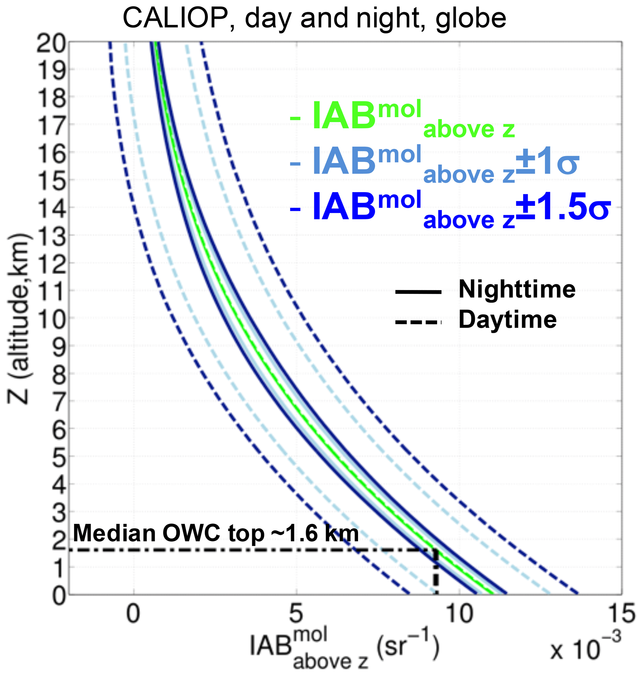
Figure B1 Nighttime (solid) and daytime (dashed) simulated vertical profile of integrated attenuated backscatter above any given altitude, z, IAB${}_{\text{above}z}^{\text{mol}}$ (green curve). The light blue (respectively dark blue) envelope shows 1 (respectively 1.5) standard deviation (σ) around the IAB${}_{\text{above}z}^{\text{mol}}$ profile. Data were generated by the CALIPSO lidar simulator (Powell et al., 2002, 2006). The IAB${}_{\text{above}z}^{\text{mol}}$ value associated with the median OWC top height of ∼1.6 km in our dataset corresponds to 0.0093 sr⁻¹.

In this study, we assume “clear air” when IAB${}_{\text{aboveCloud}}^{\text{tot}}$ is within the simulated IAB${}_{\text{aboveCloud}}^{\text{mol}}$ value ±1σ (i.e., the light blue envelope shown in Fig. B1). This definition of “clear air above” conditions is somewhat more restrictive than those imposed in previous studies. For example, Liu et al. (2015) conducted an extensive study of AAC optical depths and lidar ratios using CALIOP measurements over the tropical and southeast Atlantic. To identify clear air above cloud cases, Liu et al. (2015) require that the integrated attenuated scattering ratio, defined as

$$\begin{array}{}\text{(B5)}& {\displaystyle }\text{ASR}={\displaystyle \frac{{\int }_{\mathrm{8}\text{km}}^{{\text{OWC}}_{\text{top}}}\left({\mathit{\beta }}_{\text{m}}\left(r\right)+{\mathit{\beta }}_{\text{a}}\left(r\right)\right)T_{\text{m}}^{\mathrm{2}}(\mathrm{0},r)T_{\text{a}}^{\mathrm{2}}(\mathrm{0},r)\text{d}r}{{\int }_{\mathrm{8}\text{km}}^{{\text{OWC}}_{\text{top}}}{\mathit{\beta }}_{\text{m}}\left(r\right)T_{\text{m}}^{\mathrm{2}}(\mathrm{0},r)\text{d}r}},\end{array}$$

fall within the range of 0.95 < ASR < 1.05, irrespective of cloud top altitude. For comparison, at the maximum OWC top altitude used in our analyses (3 km), (IAB${}_{\text{aboveCloud}}^{\text{mol}}\pm \mathrm{1}\mathit{\sigma })/{\text{IAB}}_{\text{aboveCloud}}^{\text{mol}}=\mathrm{1}\pm \mathrm{0.0380}$. This restriction tightens for lower cloud top heights; e.g., at our mean OWC top altitude of 1.6 km, (IAB${}_{\text{aboveCloud}}^{\text{mol}}\pm \mathrm{1}\mathit{\sigma })/{\text{IAB}}_{\text{aboveCloud}}^{\text{mol}}=\mathrm{1}\pm \mathrm{0.0325}$.

The pioneering study by Chand et al. (2008), who first used the CALIOP DR method to assess the radiative effects of aerosols above clouds, took a different approach to identifying “clear above cloud” cases. Rather than examining the overlying IAB, they instead assumed clear air above conditions whenever IAB${}_{\text{SS}}^{\text{OWC}}>\mathrm{0.025}$ sr⁻¹. As will be shown in Appendix B3, in addition to the IAB${}_{\text{aboveCloud}}^{\text{mol}}$ limits cited above, our study also enforces limits on IAB${}_{\text{SS,CAC}}^{\text{OWC}}$. This combination of limits on both IAB${}_{\text{aboveCloud}}^{\text{mol}}$ and IAB${}_{\text{SS,CAC}}^{\text{OWC}}$ serves to more effectively reject aerosol-contaminated profiles from the “clear above” dataset than either one alone.

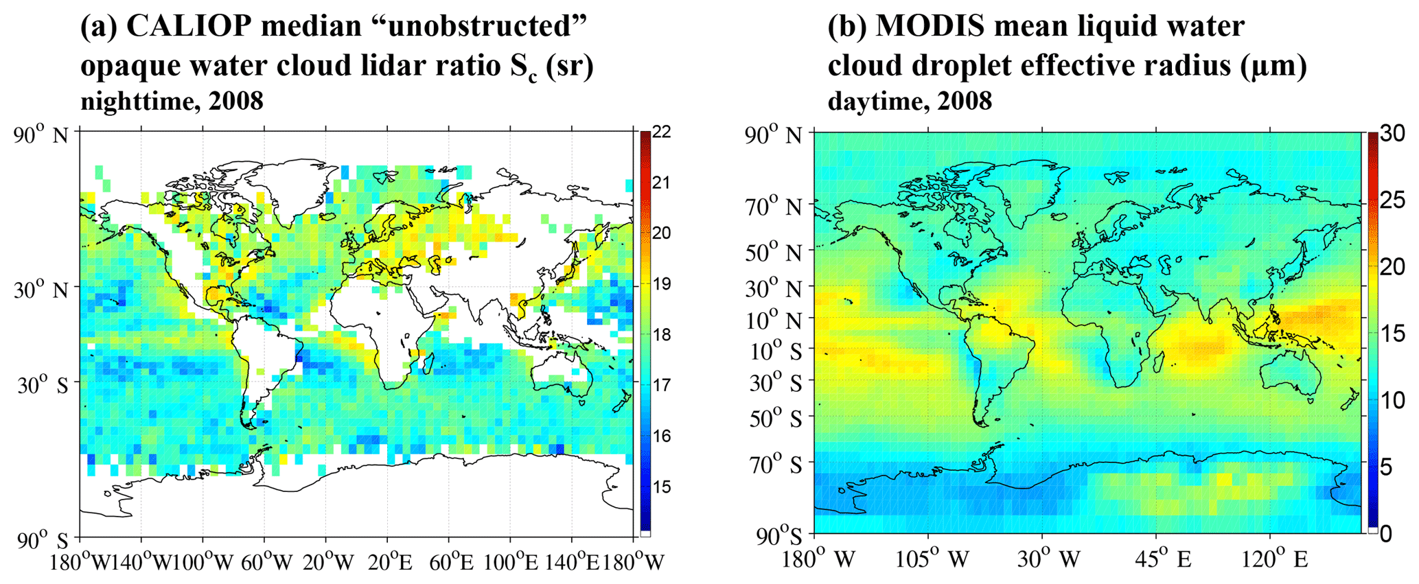
Figure B2 (a) Global CALIOP yearly median nighttime “unobstructed” (i.e., clear air above) OWC lidar ratio, S_c, in 2008 that satisfies all criteria of Table B2. For the reasons outlined in this section, any OWC along the CALIOP track for which S_c>20 sr or S_c<14 sr is deleted before temporal and spatial averaging. White pixels show a limited number of OWCs; (b) Global MODIS yearly mean daytime liquid water cloud droplet effective radius, R_e (in µm, “Cloud Effective Radius Liquid Mean Mean” parameter from MODIS MYD08_M3 product).

B3 Process median seasonal maps of integrated attenuated backscatter of opaque water clouds showing clear air above

Once we select specific OWCs (i.e., that satisfy the criteria of Table B2) and define which ones are “unobstructed” (see Appendix B2), we can easily compute IAB${}_{\text{SS,CAC}}^{\text{OWC}}$ by using Eq. (B3). For clouds that totally attenuate the lidar signal (i.e., cloud optical depths greater than ∼6; Young et al., 2018), IAB${}_{\text{SS,CAC}}^{\text{OWC}}$ in Eq. (2) or (B1) is related to the OWC lidar ratio (called S_c), so that

$$\begin{array}{}\text{(B6)}& {\displaystyle }{S}_{\text{c}}=\mathrm{1}/\left(\mathrm{2}\times {\mathit{\eta }}^{\text{OWC}}\times {\text{IAB}}_{\text{CAC}}^{\text{OWC}}\right)=\mathrm{1}/\left(\mathrm{2}\times {\text{IAB}}_{\text{SS,CAC}}^{\text{OWC}}\right)\end{array}$$

(Platt, 1973). OWC S_c values are relatively stable at the visible and near-infrared wavelengths (Pinnick et al., 1983; O'Connor et al., 2004) but show large variations over land (Pinnick et al., 1983; Hu et al., 2006). S_c is known to vary as a function of cloud droplet microphysics, and is especially sensitive to cloud droplet effective radius (R_e) and the imaginary part of the refractive index (see Fig. 8 of Deaconu et al., 2017). Hu et al. (2006), Liu et al. (2015) and Deaconu et al. (2017) show that a decrease in R_e is often paired with an increase in estimated S_c at 532 nm for pure, non-aerosol-contaminated water clouds (i.e., cloud droplets having an imaginary refractive index of 0).

As an example, Fig. B2a shows the median nighttime CALIOP S_c values across the globe during 2008. Figure B2b shows MODIS AQUA-derived mean liquid water R_e in 2008 (using MODIS Level 3 monthly product “Cloud Effective Radius Liquid Mean Mean”).

Greater S_c values paired with lower cloud R_e can be seen offshore and close to the west coasts of Africa and the Americas in Fig. B2. Other notable regions of low cloud R_e and high S_c in Figure B2 are above industrial regions like northern Europe, the eastern US and Southeast Asia. These results appear to support Twomey's analysis (Twomey, 1977; Rosenfeld and Lensky, 1998), showing an enhancement of the cloud albedo through the increase in droplet number concentration and a decrease in the droplet size driven by increased aerosol concentration. On the other hand, Fig. B2a mostly exhibits low S_c values (paired with large R_e) over the inter-tropical convergence zone (ITCZ), likely associated with deep convective regimes. In addition, Fig. B2a generally shows larger OWC S_c values in the Northern Hemisphere than in the Southern Hemisphere, which we attribute to differences in sources of cloud condensation nuclei. Figure B2b shows patterns that are generally similar to those in Fig. B2a, but of opposite intensity. Let us note that the polarization measurements from the space-borne POLDER sensor (Deschamps et al., 1994) were also used to estimate R_e of liquid water clouds across the globe (Bréon and Colzy, 2000) and seem to be in qualitative agreement with the findings of Fig. B2b.

During our assessment of 5 years of CALIOP data across the globe, we have observed significantly higher “unobstructed” OWC S_c values (i.e., S_c>20 sr, not shown in Fig. B2a) near the coasts of West Africa and over the region of SE Asia (e.g., see Young et al., 2018). These may be physically plausible and either (1) associated with small cloud R_e, resulting from the Twomey's effect as explained above, or (2) associated with the presence of light-absorbing aerosols residing within the OWCs (Mishchenko et al., 2014; Chylek and Hallett, 1992; Wittbom et al., 2014). These aerosols would be undetected in our IAB${}_{\text{aboveCloud}}^{\text{mol}}$ clear air selection method (see Appendix B2) and would impact the chemical composition of the cloud droplets, modifying their backscattered light. The latter is well illustrated in Fig. 8 of Deaconu et al. (2017), which shows simulations of cloud S_c with an imaginary part of the refraction index equal to 0.0001, as a function of cloud droplet effective radius. Other reasons for these unusually high S_c values could be the sources of uncertainty noted (a), (b), (c) and (d) in the beginning of Appendix B, with (c) (i.e., the SNR of the backscatter data within the layer) possibly having a much higher impact on S_c than all other factors. An additional source of uncertainty on the retrieval of S_c could be a failure of the CALIPSO surface detection scheme. If CALIOP fails to detect the surface adequately, part of the Earth's surface could be misclassified as an opaque water cloud and these misclassified clouds would have abnormally high S_c.

Let us note that the vast majority of the S_c values reported in the literature (i.e., in Hu et al., 2006; Liu et al., 2015; Deaconu et al., 2017) are estimated using a Mie code and not directly measured. However, none of these results show S_c values above 20 sr for non-aerosol-contaminated OWCs. On the other hand (and to add a lower bracket on our OWC S_c calculations), none of these results show S_c values below 14 sr. For this reason, we have imposed an additional threshold on the OWC S_c values as part of step (S3) in Table B1: we delete any “unobstructed” OWC along the CALIOP track for which S_c>20 sr (i.e., unrealistically small water cloud droplets) or S_c<14 sr (i.e., unrealistically large water cloud droplets). Every OWC S_c value along the CALIOP track was then compiled to produce four global median seasonal $\mathrm{4}{}^{\circ }\times \mathrm{5}{}^{\circ }$ maps of OWC S_c using 5 years of nighttime CALIOP data (from 2008 to 2012).

There is additional precedent for establishing an upper limit of S_c=20 sr. Note that, from Eq. (B6), the value of IAB${}_{\text{SS,CAC}}^{\text{OWC}}$ corresponding to S_c=20 sr is 0.025 sr⁻¹. As mentioned earlier, this is the same OWC IAB threshold value used by Chand et al. (2008) to identify their “clear air above” cases.

Appendix C: Acronyms

AAC	Aerosol above clouds
AAOD	Absorption aerosol optical depth
AOD	Aerosol optical depth
${\mathit{\tau }}_{\text{AAC}}^{\text{DR}}$	Aerosol optical depth above clouds using the DR method
AeroCom	Aerosol Comparisons between Observations and Models
AERONET	AErosol RObotic NETwork
AMSR-E	Advanced Microwave Scanning Radiometer - Earth Observing System
ARCTAS	Arctic Research of the Composition of the Troposphere from Aircraft and Satellites
ASR	integrated Attenuated Scattering Ratio
BRDF	Bidirectional Reflectance Distribution Function
CAC	Clear air above cloud
CALIOP	Cloud–Aerosol Lidar with Orthogonal Polarization
CALIPSO	Cloud–Aerosol Lidar and Infrared Pathfinder Satellite Observations
CERES	Clouds and the Earth's Radiant Energy System
CF	Cloud fraction
CloudSat	NASA Earth observation satellite
COD	Cloud optical depth
CR	Color ratio technique
DAREall-sky	Direct aerosol radiative effect in all-sky conditions (cloudy and non-cloudy)
DAREcloudy	Direct aerosol radiative effect in cloudy conditions
DAREnon-cloudy	Direct aerosol radiative effect in non-cloudy conditions (clear-skies)
DAREOWC	Direct aerosol radiative effect above opaque water clouds
DISORT	DIScrete ORdinate Radiative Transfer solvers
DR	Depolarization Ratio technique
δOWC	Layer-integrated volume depolarization ratio
fAAC	AAC frequency of occurrence
HSRL	High spectral resolution lidar
IAB	Integrated attenuated backscatter
IBS	Integrated aerosol backscatter
InWA	Indian ocean, offshore from western Australia
LUT	Look-up table
LWP	Liquid water path
MBL	Marine boundary layer
MCD43GF	MODIS BRDF/Albedo/NBAR CMG gap-filled products
MODIS	MODerate Imaging Spectroradiometer
ηOWC	Layer effective multiple scattering factor
NEAs	Northeast Asia
NEPa	Northeast Pacific ocean
NWPa	Northwest Pacific ocean
OMI	Ozone Monitoring Instrument
ORACLES	ObseRvations of Aerosols above CLouds and their intEractionS
OWC	Opaque water cloud
POLDER	Polarization and Directionality of Earth's Reflectances
PBL	Planetary boundary layer
Re	Cloud droplet effective radius
RT	Radiative transfer scheme
Sa	Aerosol extinction-to-backscatter (lidar) ratio
Sc	Cloud extinction-to-backscatter (lidar) ratio
SCIAMACHY	Scanning Imaging Absorption Spectrometer for Atmospheric Cartography
SEAs	Southeast Asia
SEAt	Southeast Atlantic ocean
SEPa	Southeast Pacific ocean

SEVIRI	Spinning Enhanced Visible and InfraRed Imager
SNR	Signal-to-noise ratio
SS	Single scattering
SSA	Single scattering albedo
SW	Shortwave
TAt	Tropical Atlantic ocean
TOA	Top of atmosphere