the Creative Commons Attribution 4.0 License.
the Creative Commons Attribution 4.0 License.
 | 10 Apr 2019
Evaluation of CESM1 (WACCM) free-running and specified dynamics atmospheric composition simulations using global multispecies satellite data records
Lucien Froidevaux
Douglas E. Kinnison
John Anderson
Ryan A. Fuller
We have analyzed near-global stratospheric data (and mesospheric data as well for H2O) in terms of absolute abundances, variability, and trends for O3, H2O, HCl, N2O, and HNO3, based on Aura Microwave Limb Sounder (MLS) data, as well as longer-term series from the Global OZone Chemistry And Related trace gas Data records for the Stratosphere (GOZCARDS). While we emphasize the evaluation of stratospheric models via data comparisons through 2014 to free-running (FR-WACCM) and specified dynamics (SD-WACCM) versions of the Community Earth System Model version 1 (CESM1) Whole Atmosphere Community Climate Model (WACCM), we also highlight observed stratospheric changes, using the most recent data from MLS.
Regarding highlights from the satellite data, we have used multiple linear regression to derive trends based on zonal mean time series from Aura MLS data alone, between 60∘ S and 60∘ N. In the upper stratosphere, MLS O3 shows increases over 2005–2018 at ∼0.1–0.3 % yr−1 (depending on altitude and latitude) with 2σ errors of ∼0.2 % yr−1. For the lower stratosphere (LS), GOZCARDS O3 data for 1998–2014 point to small decreases between 60∘ S and 60∘ N, but the trends are more positive if the starting year is 2005. Southern midlatitudes (30–60∘ S) exhibit near-zero or slightly positive LS trends for 1998–2018. The LS O3 trends based on 2005–2018 MLS data are most positive (0.1–0.2 % yr−1) at these southern midlatitudes, although marginally statistically significant, in contrast to slightly negative or near-zero trends for 2005–2014. Given the high variability in LS O3, and the high sensitivity of trends to the choice of years used, especially for short periods, further studies are required for a robust longer-term LS trend result. For H2O, upper-stratospheric and mesospheric trends from GOZCARDS 1992–2010 data are near zero (within ∼0.2 % yr−1) and significantly smaller than trends (within ∼0.4–0.7 % yr−1) from MLS for 2005–2014 or 2005–2018. The latter short-term positive H2O trends are larger than expected from changes resulting from long-term increases in methane. We note that the very shallow solar flux maximum of solar cycle 24 has contributed to fairly large short-term mesospheric and upper-stratospheric H2O trends since 2005. However, given known drifts in the MLS H2O time series, MLS H2O trend results, especially after 2010, should be viewed as upper limits. The MLS data also show regions and periods of small HCl increases in the lower stratosphere, within the context of the longer-term stratospheric decrease in HCl, as well as interhemispheric–latitudinal differences in short-term HCl tendencies. We observe similarities in such short-term tendencies, and interhemispheric asymmetries therein, for lower-stratospheric HCl and HNO3, while N2O trend profiles exhibit anti-correlated patterns.
In terms of the model evaluation, climatological averages for 2005–2014 from both FR-WACCM and SD-WACCM for O3, H2O, HCl, N2O, and HNO3 compare favorably with Aura MLS data averages over this period. However, the models at mid- to high latitudes overestimate mean MLS LS O3 values and seasonal amplitudes by as much as 50 %–60 %; such differences appear to implicate, in part, a transport-related model issue. At lower-stratospheric high southern latitudes, variations in polar winter and spring composition observed by MLS are well matched by SD-WACCM, with the main exception being for the early winter rate of decrease in HCl, which is too slow in the model. In general, we find that the latitude–pressure distributions of annual and semiannual oscillation amplitudes derived from MLS data are properly captured by the model amplitudes. In terms of closeness of fit diagnostics for model–data anomaly series, not surprisingly, SD-WACCM (driven by realistic dynamics) generally matches the observations better than FR-WACCM does. We also use root mean square variability as a more valuable metric to evaluate model–data differences. We find, most notably, that FR-WACCM underestimates observed interannual variability for H2O; this has implications for the time period needed to detect small trends, based on model predictions.
The WACCM O3 trends generally agree (within 2σ uncertainties) with the MLS data trends, although LS trends are typically not statistically different from zero. The MLS O3 trend dependence on latitude and pressure is matched quite well by the SD-WACCM results. For H2O, MLS and SD-WACCM positive trends agree fairly well, but FR-WACCM shows significantly smaller increases; this discrepancy for FR-WACCM is even more pronounced for longer-term GOZCARDS H2O records. The larger discrepancies for FR-WACCM likely arise from its poorer correlations with cold point temperatures and with quasi-biennial oscillation (QBO) variability. For HCl, while some expected decreases in the global LS are seen in the observations, there are interhemispheric differences in the trends, and increasing tendencies are suggested in tropical MLS data at 68 hPa, where there is only a slight positive trend in SD-WACCM. Although the vertical gradients in MLS HCl trends are well duplicated by SD-WACCM, the model trends are always somewhat more negative; this deserves further investigation. The original MLS N2O product time series yield small positive LS tropical trends (2005–2012), consistent with models and with rates of increase in tropospheric N2O. However, longer-term series from the more current MLS N2O standard product are affected by instrument-related drifts that have also impacted MLS H2O. The LS short-term trend profiles from MLS N2O and HNO3 at midlatitudes in the two hemispheres have different signs; these patterns are well matched by SD-WACCM trends for these species.
These model–data comparisons provide a reminder that the QBO and other dynamical factors affect decadal variability in a major way, notably in the lower stratosphere, and can thus significantly hinder the goals of robustly extracting (and explaining) small underlying long-term trends. The data sets and tools discussed here for model evaluation could be expanded to comparisons of species or regions not included here, as well as to comparisons between a variety of chemistry–climate models.
- Article
(27203 KB) - Full-text XML
-
Supplement
(1734 KB) - BibTeX
- EndNote


The author's copyright for this publication is transferred to California Institute of Technology.
State-of-the-art chemistry–climate models (CCMs) are known to reproduce the main features of stratospheric climatology and change, although there have always been some differences between models (e.g., Waugh and Eyring, 2008; SPARC, 2010; Dhomse et al., 2018). Free-running CCMs are used to make long-term simulations of atmospheric composition, as well as predictions of future changes, driven by time-dependent boundary conditions for surface concentrations of greenhouse gases and ozone-depleting substances (ODSs), sea surface temperatures and sea ice concentrations, 11-year solar variability, sulfate aerosol surface area density, and tropospheric ozone and aerosol precursor emissions. In more recent years, modeling groups have implemented “specified dynamics” versions that are constrained to meteorological fields (e.g., surface pressure, temperature, and winds). Our main purpose is to evaluate these two types of model runs from CESM1 WACCM, using multispecies satellite-derived global composition data sets; we refer to these two types as FR-WACCM (free-running model) and SD-WACCM (specified dynamics version). The SD-WACCM version has been used in studies ranging from examination of ozone trends (e.g., Solomon et al., 2016; Ball et al., 2017; Wilka et al., 2018) to evaluation of galactic cosmic ray influence on ozone (Jackman et al., 2016). This configuration has also been used to study dynamical processes that affect stratospheric ozone (e.g., Khosrawi et al., 2013; Gille et al., 2014) and has contributed to the understanding of satellite occultation instrument differences (Sakazaki et al., 2015). Here, we perform a detailed model/observational analysis of two configurations (FR and SD) using the same modeling system (CESM) and identical tracer advection and chemistry modules. Differences between the two configurations should be caused mainly by the influence of different temperature fields on chemistry and by different mean circulations. The simulations are based on scenarios defined by the Chemistry-Climate Model Initiative (CCMI) (Eyring et al., 2013; Morgenstern et al., 2017). Our evaluation focus is on monthly zonal mean series from the models versus satellite-derived data. The main stratospheric series used here are from Aura Microwave Limb Sounder (MLS) data (version 4.2) and from the Global OZone Chemistry And Related trace gas Data records for the Stratosphere (GOZCARDS), which include MLS data from late 2004 onward. GOZCARDS includes merged multi-satellite data files for O3, H2O, and HCl, as well as Aura MLS data for HNO3 and N2O; these five species are used for the evaluations. We focus, in part, on the MLS data sets for 2005–2014 (2014 being the last year of WACCM runs considered here). The regular and nearly uninterrupted daily global coverage of the MLS day and night measurements leads to minimal sampling-related biases, both for climatological comparisons (Toohey et al., 2013) and trend-related studies. This data set also has a well characterized set of error bars (see Livesey et al., 2018, for the latest update to the data quality documentation); however, we also note that there are some caveats to take into account regarding long-term stability for some of the MLS species.
In terms of model–data comparisons, we analyze the climatological mean state and goodness-of-fit issues, as well as variability. While one has the expectation that, in general, better fits to the data would be obtained for a specified dynamics run than for a less dynamically constrained run (FR-WACCM), one needs to demonstrate this with diagnostics that provide enough differentiation between models that can track each other closely. There have been essentially no trend studies using Aura MLS data by themselves. This data set now covers a sufficiently long period that it becomes useful to investigate such trends, as the analyses deal with one data set only, which can remove potential issues with data merging prior to 2005, whether related to poorer sampling or to uncertainties in bias removal between data sets. While such uncertainties can be difficult to quantify, attempts have been made in the case of ozone data merging from multiple SBUV (Solar Backscatter Ultraviolet Radiometer) instruments, which display relative biases and drifts (Frith et al., 2017); data merging uncertainties in this case were shown to play a large role regarding overall trend uncertainties. Regarding sampling issues, Millán et al. (2016) showed, based on simulated atmospheric fields, that solar occultation-type sampling can significantly bias trend results, as well as increase the time period required for robust trend detection, compared to emission-type (much denser) sampling. On the downside, a shorter time series will lead to larger uncertainties in derived trends.
We provide (in Sect. 2) an overview of the global stratospheric data sets used here. Brief descriptions of FR-WACCM and SD-WACCM are given in Sect. 3. Climatological comparisons between models and Aura MLS data are provided in Sect. 4, in order to assess whether any obvious biases exist; this includes an overview of the main short-term variations, namely the annual oscillation (AO) and semiannual oscillation (SAO). More detailed comparisons of deseasonalized anomaly time series are provided in Sect. 5.1, where we evaluate how well the two model versions fit the data sets, both in terms of closeness of fits and variability. Trend results and comparisons are provided in Sect. 5.2, before the closing summary and discussion in Sect. 6.
2.1 Aura MLS
The Microwave Limb Sounder (MLS) is one of four instruments on NASA's Aura satellite, launched on 15 July 2004. The MLS antenna scans the atmospheric limb as Aura orbits the Earth in a near-polar sun-synchronous orbit, and the instrument measures thermal emission (day and night) in narrow spectral channels, via microwave radiometers operating at frequencies near 118, 190, 240, and 640 GHz, as well as a 2.5 THz module to measure OH. MLS (see Waters et al., 2006) has been providing a variety of daily vertical stratospheric temperature and composition profiles (∼3500 profiles per day per product), with some measurements extending down to the upper tropospheric region and some into the upper mesosphere or higher. For more information and access to the MLS data, the reader is referred to http://disc.sci.gsfc.nasa.gov/Aura/data-holdings/MLS, last access: 4 April 2019; the current data version is labeled 4.2x (with x varying between 0 and 3, depending on the date). Data users interested in MLS data quality and characterization, estimated errors, and related information should consult Livesey et al. (2018), the latest update to the MLS data quality document (available from the MLS website at http://mls.jpl.nasa.gov, last access: 4 April 2019).
2.2 GOZCARDS
The data set considered here for longer-term model evaluation analyses is from GOZCARDS, a data record created using satellite-based Level 2 data as source data sets, which were merged into global monthly zonal means for O3, H2O, and HCl, going back in time before the (2004) launch of Aura. Readers are referred to the GOZCARDS description and highlights provided by Froidevaux et al. (2015). In brief, for O3, the GOZCARDS version 1.01 (v1.01) data record starts in 1979 with solar occultation data from the first Stratospheric Aerosol and Gas Experiment (SAGE I) and continues with data from SAGE II, the Halogen Occultation Experiment (HALOE), the Upper Atmosphere Research Satellite (UARS) MLS, the Atmospheric Chemistry Experiment Fourier Transform Spectrometer (ACE-FTS, using solar occultation), and Aura MLS. Basically, the overlap time periods for different data sets are used to calculate offsets between zonal mean time series in 10∘ wide latitude bins at each pressure level, and the data sets are adjusted to a reference value (SAGE II mean values, for O3, or an average of satellite measurements for H2O and HCl). Monthly standard deviations are also provided, along with other diagnostic quantities. GOZCARDS data extensions past 2012 were created simply by adding more recent MLS data, appropriately adjusted to account for zonal mean differences between versions, once the MLS O3 v2.2 data became unavailable (for 2013 onward); ACE-FTS data were not included in these more recent years. GOZCARDS O3 has been used for past O3 trend assessments and in comparisons to other data records (e.g., WMO, 2014; Nair et al., 2015; Tummon et al., 2015; Harris et al., 2015; Ball et al., 2017, 2018).
For the GOZCARDS O3 data discussed here, unless otherwise noted, we use GOZCARDS v2.20, a recent improvement and update to the original version. This data set was provided for an updated assessment of stratospheric ozone by Steinbrecht et al. (2017), as well as for the assessment activities of the Long-term Ozone Trends and Uncertainties in the Stratosphere (LOTUS) project and in preparation for the latest international report on the state of the ozone layer, led by the World Meteorological Organization (WMO). GOZCARDS ozone data updates are also used as part of the yearly “State of the Climate” stratospheric ozone-related summaries, produced for the Bulletin of the American Meteorological Society (BAMS). For GOZCARDS O3 v2.20, the stratospheric retrieval pressure grid is twice as fine as for v1.01; there are now 12 regularly spaced levels per decade change in log of pressure. UARS MLS O3 data were not included in v2.20, since these retrievals are not readily available on the finer vertical grid (although approximations such as interpolation could be used); also, there is no easy provision of UARS MLS retrieval uncertainties on a finer grid. The most significant change for the new merged O3 is the effect of using the more robust version 7 data from SAGE II (Damadeo et al., 2013). Version 7 uses National Aeronautics and Space Administration (NASA) Global Modeling and Assimilation Office (GMAO) Modern-Era Retrospective Analysis for Research and Applications (MERRA) temperature (T) profile data (Rienecker et al., 2011) in the retrievals, and these values (rather than T from the National Centers for Environmental Prediction, NCEP) also have a significant impact on the conversion of SAGE II O3 from its native density–altitude grid to the GOZCARDS mixing-ratio–pressure grid. Also, Aura MLS v4.2 O3 data are now used (instead of MLS v2.2); HALOE v19 O3 profiles are included after interpolation to the finer pressure grid before merging. As a result of these changes, we have observed closer agreement and larger correlation coefficients between the Stratospheric Water and Ozone Satellite Homogenized (SWOOSH) ozone data (Davis et al., 2016) and GOZCARDS v2.20 O3 series than between SWOOSH and GOZCARDS v1.01 (SWOOSH also uses SAGE II v7 O3 data). More details regarding the impact of GOZCARDS v2.20 O3 on trends are provided in Sect. 5. We note that no ACE-FTS data were included in this newer version of GOZCARDS O3.
WACCM (CESM1) is a chemistry–climate model of the Earth's atmosphere, from the surface to the lower thermosphere (Garcia et al., 2007, 2017; Kinnison et al., 2007; Marsh et al., 2013). WACCM is a superset of the Community Atmosphere Model, version 4 (CAM4), and includes all of the physical parameterizations of CAM4 (Neale et al., 2013) and a finite volume dynamical core (Lin, 2004) for the tracer advection. The horizontal resolution is 1.9∘ latitude × 2.5∘ longitude. The vertical resolution in the lower stratosphere (LS) ranges from 1.2 km near the tropopause to ∼2 km near the stratopause; in the mesosphere and thermosphere the vertical resolution is ∼3 km. Simulations used here are based on the guidelines from the International Global Atmospheric Chemistry – Stratosphere-troposphere Processes And their role in Climate (IGAC/SPARC) Chemistry-Climate Model Initiative (Morgenstern et al., 2017). Improvements in CESM1 WACCM for CCMI include a modification to the orographic gravity wave forcing, which reduced the cold bias in Antarctic polar temperatures (Garcia et al., 2017; Calvo et al., 2017), and updates to the stratospheric heterogeneous chemistry, which improved the representation of polar ozone depletion (Wegner et al., 2013; Solomon et al., 2015). In this work, there are two CCMI scenarios, spanning the 1990–2014 period. The first scenario follows the CCMI REF-C1 definition and three ensemble members were completed; this falls under the free-running scenario. We note that all the analyses herein are based on an average of these three simulations. We have checked that the three representations' departures from the average are small enough not to require separate comparisons for each case, when pursuing average or root mean square (rms) differences versus observations, in comparison to differences using the second model scenario (see below); this is also true for the model–data comparisons of rms variability. This first model scenario includes forcing from greenhouse gases (CH4, N2O, and CO2), organic halogens, volcanic aerosol surface area density and heating, and 11-year solar cycle variability. The sea surface temperatures are based on observations and the quasi-biennial oscillation (QBO) is nudged to observed monthly mean tropical winds over 86–4 hPa, as described in Matthes et al. (2010).
The second scenario is based on the CCMI REF-C1SD scenario and includes all the forcings of REF-C1, except for additional external QBO nudging. This scenario uses the specified dynamics (SD) option in WACCM (Lamarque et al., 2012). Here, temperature, zonal and meridional winds, and surface pressure are used to drive the physical parameterization controlling boundary layer exchanges, advective and convective transport, and the hydrological cycle. The meteorological analyses are taken from MERRA and the nudging approach is described in Kunz et al. (2011). The QBO circulation is inherent in the MERRA meteorological fields and is therefore synchronized with that in the real atmosphere. The horizontal resolution is the same as the REF-C1 version, and the vertical resolution follows the MERRA reanalysis (from ∼1 km resolution near the tropopause to about 2 km near the stratopause). The model meteorological fields are nudged from the surface to 50 km; above 60 km, these fields are fully interactive, with a linear transition in between.
Both WACCM versions used here contain an identical representation of tropospheric and stratospheric chemistry (Kinnison et al., 2007; Tilmes et al., 2016). The species included in this mechanism are contained within the Ox, NOx, HOx, ClOx, and BrOx chemical families, along with CH4 and its degradation products. In addition, 20 primary non-methane hydrocarbons and related oxygenated organic compounds are represented, along with their surface emissions. In total there are 183 species and 472 chemical reactions; this includes 17 heterogeneous reactions on multiple aerosol types (i.e., sulfate, nitric acid trihydrate, and water–ice). For this work, the CESM1 (WACCM) REF-C1 and REF-C1SD simulations will generally be referred to as FR-WACCM and SD-WACCM, respectively. While the runs were originally designed to stop at the end of 2010, for this work, the forcing inputs have been extended through 2014.
We first describe some of the major climatological features for the stratospheric species mentioned in the Introduction. We focus on the main differences between average model trace gas abundances from FR-WACCM and SD-WACCM and the corresponding data from Aura MLS for 2005 through 2014; this includes a subsection on annual and semiannual variations.
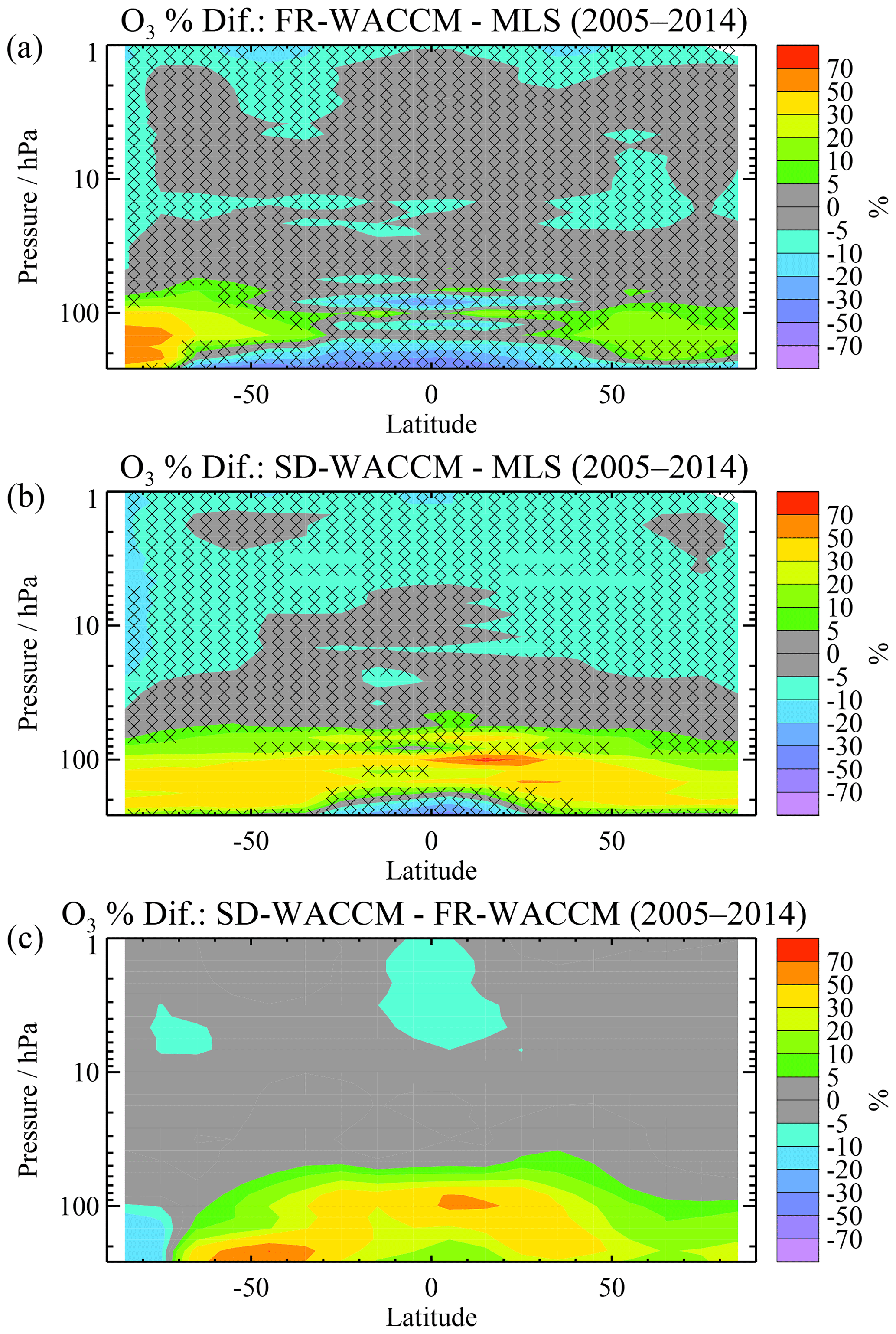
Figure 1These latitude–pressure contour plots show percent differences (100 × (model-data) ∕ data) for binned climatological O3 from 2005 to 2014 (see Fig. S1 for the average MLS and model values), for (a) the free-running model (average of three FR-WACCM realizations), (b) for the specified dynamics (SD-WACCM) version, and (c) for SD-WACCM – FR-WACCM. Regions that are not crossed out in (a) and (b) are regions where the model climatology differs quite significantly from the data, based on a comparison of the ratio of (absolute) model–data differences to MLS systematic error estimates (see text).
4.1 Average abundances
We provide climatological latitude–pressure contour plots in the Supplement (Fig. S1 for O3 and H2O; Fig. S2 for HCl, HNO3, and N2O), showing Aura MLS and WACCM average distributions for 2005–2014. Since such plots do not easily allow one to quantify areas of model–data disagreement, we show in Fig. 1a and b the percent differences between WACCM and MLS climatologies; a positive value means that, on average, the model values exceed the data values. Figure 1c provides a comparison between the models (also as percent differences). We have crossed out the regions in Fig. 1a and b where there is little statistical significance in the model–data differences; more specifically, this is where the absolute differences are less than 1.5 times the systematic uncertainties in MLS abundances. These error estimates have been provided in MLS validation and error characterization work as “typical” (global) profiles versus pressure; such estimates for version 4 MLS data are provided by Livesey et al. (2018) and are typically 2σ estimates; thus, regions with the most significant differences (above the 3σ error level) are shown without crosses. The vertical profile of MLS O3 systematic errors is given in the Supplement (Fig. S3). Past validation references for MLS O3 include Jiang et al. (2007), Froidevaux et al. (2008a), and Livesey et al. (2008), as well as the more recent work covering many satellite instruments by Hubert et al. (2016). The original MLS data validation work for H2O is from Read et al. (2007) and Lambert et al. (2007), who also described N2O validation; MLS HNO3 validation was provided by Santee et al. (2007). Based on Fig. 1, most of the model O3 climatology falls within 5 % to 10 % of the data climatology, except in the upper troposphere and lower stratosphere (UTLS), where SD-WACCM O3 values are even larger than those from FR-WACCM (Fig. 1c). Our work focuses on the stratosphere, but both FR-WACCM and SD-WACCM average O3 values at low latitudes are lower than the observed means from 215 to 261 hPa (and these levels lie in the upper troposphere at these latitudes); in this region, there are known MLS positive biases versus tropical ozonesonde data, and this could account for part of the apparent model low bias. However, midlatitude O3 from 100 to 215 hPa is biased high in SD-WACCM, with a difference to systematic error ratio larger than 2 to 3. An illustration of the more significant differences is given in Fig. 2 for O3 data and model series at 215 hPa for 50–60∘ N (which corresponds to lower-stratospheric values). This shows that both FR-WACCM and SD-WACCM values are larger than the data there, and more so for SD-WACCM, for which the overestimate can be larger than 50 %. In relation to this, Imai et al. (2013) showed that SD-WACCM O3 values are also larger than Superconducting Submillimeter-Wave Limb-Emission Sounder (SMILES) O3 in the lowest portion of the stratosphere (18–20 km). In Fig. 2, we also see that the model O3 annual amplitude (AO) is larger than the observed amplitude; both models overestimate seasonal amplitudes by ∼60 %. We discuss the AO more generally in the next section. If anything, MLS O3 at midlatitudes is slightly high (by ∼5 %) with respect to a multi-instrument mean based on a number of satellite data sets from the Stratosphere-Troposphere Processes And their Role in Climate (SPARC) Data Initiative (DI), as discussed by Tegtmeier et al. (2013), who also showed that the MLS O3 seasonal cycle at midlatitudes and 200 hPa is in good agreement with the multi-instrument mean. The MLS measurements discussed here provide generally strongly peaked averaging kernels with a resolution of 2.5 to 4 km (see Livesey et al., 2018, for sample kernel plots). Smoothing the model profiles using the MLS averaging kernels (and a priori information) gives very little change (less than a few percent for the Fig. 2 example, and even less at higher altitudes) in O3 abundances and seasonal cycles, and we see no real need to use such smoothing for our comparisons. The significant model–data differences in Figs. 1 and 2 are not caused by this sort of issue. The midlatitude O3 differences mentioned above require more detailed investigations but appear to implicate (in part) a transport-related issue in these models.
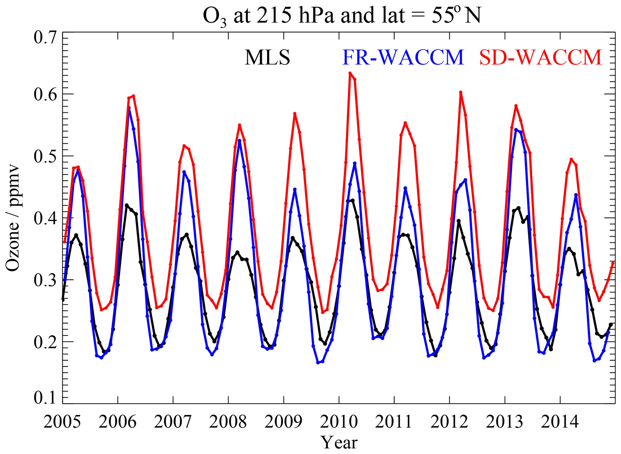
Figure 2Monthly mean ozone time series at 215 hPa and the 55∘ N latitude bin (for averages over 50–60∘ N) from MLS, FR-WACCM, and SD-WACCM (see legend for color coding).
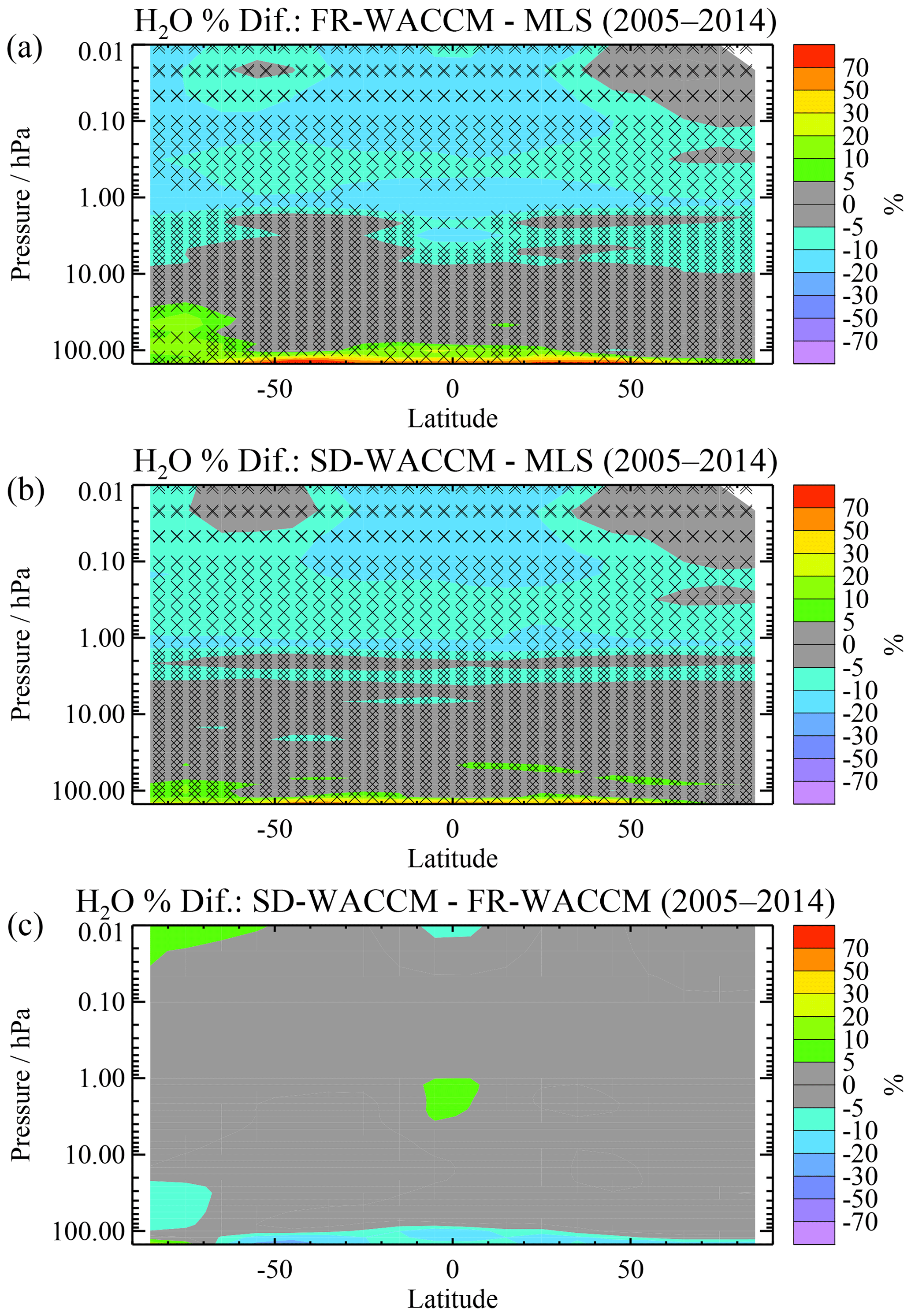
Figure 3 is the H2O analog of Fig. 1 but for pressures reaching up to 0.01 hPa; again, a typical profile of MLS systematic error estimates (Livesey et al., 2018) was used to define regions with the most statistically significant model–data differences; there are almost no such regions in Fig. 3. We note that MLS H2O v3 stratospheric data exhibit a slight high bias (of a few to 5 %) versus multi-instrument means, with a somewhat larger positive bias (of ∼10 %) in the lower mesosphere (Hegglin et al., 2013). Such biases are within the expected measurement systematic errors. MLS version 4 stratospheric H2O data show essentially no systematic change versus version 3 (Livesey et al., 2018). FR-WACCM and SD-WACCM H2O mean values are on the low side (by ∼5–15 %) relative to MLS H2O in the upper stratosphere and in most of the mesosphere (see Fig. 3), implying that the models are in good agreement with the SPARC DI multi-instrument mean H2O. There is independent evidence that MLS H2O has a dry bias near the hygropause (at the low end of the vertical range shown in Fig. 3, where the bottom level is 150 hPa); this has been known for some time (Read et al., 2007; Vömel et al., 2007). This is also consistent with the existence of a model high bias relative to MLS near 150 hPa. The H2O model–data comparisons are generally in agreement within the systematic errors, and the level of agreement is slightly better in the case of SD-WACCM.
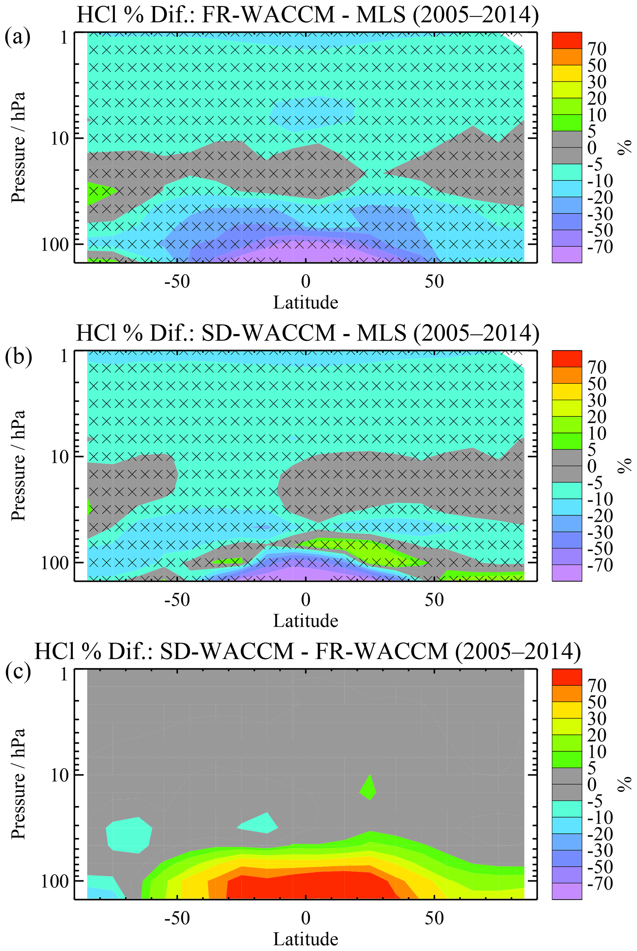
For HCl, the climatological comparisons of Fig. 4 show that both models exhibit a small (5 %–10 %) low bias versus MLS HCl in much of the stratosphere, with a stronger negative model bias in the tropics between 100 and 150 hPa. The model–data relative biases in stratospheric HCl are generally within the MLS HCl systematic errors. MLS HCl is slightly on the high side of multi-instrument mean climatological results provided in the SPARC DI report (SPARC, 2017). The small negative model bias in the upper stratosphere could also arise from the lack of a sufficiently pronounced decrease in upper-stratospheric MLS HCl, as a result of the interruption in the main MLS HCl (band 13) data after early 2006 (Livesey et al., 2018). There is also a known positive bias in MLS tropical HCl at 150 hPa (Froidevaux et al., 2008b), so model underestimates in this region are not a sign of model weakness. We also note that both models exhibit a systematic difference versus LS HCl observations (with larger differences for SD-WACCM), as well as a downward sloping pattern (equator to pole) in the Southern Hemisphere (SH) and smaller mean differences (for SD-WACCM) in the Northern Hemisphere (NH).

Figure 5 provides average comparisons for N2O; this species is long-lived in the lower stratosphere, which means that good (or poor) model–data agreement in this region can confirm (or deny) accurate model representations of the dynamics. While mean lower-stratospheric SH N2O values are larger for SD-WACCM than for FR-WACCM (Fig. 5c), the mean fit for SD-WACCM is not significantly better. The most significant climatological differences with respect to the error bars are in the upper stratosphere at low latitudes; in this region, SD-WACCM agrees somewhat better with MLS. However, this is also where the data values decline with height, towards the limits of the MLS sensitivity. Not too surprisingly, this is also where the SPARC DI results for N2O show the largest scatter in terms of percent differences (often exceeding 10 %–20 %; see SPARC, 2017).
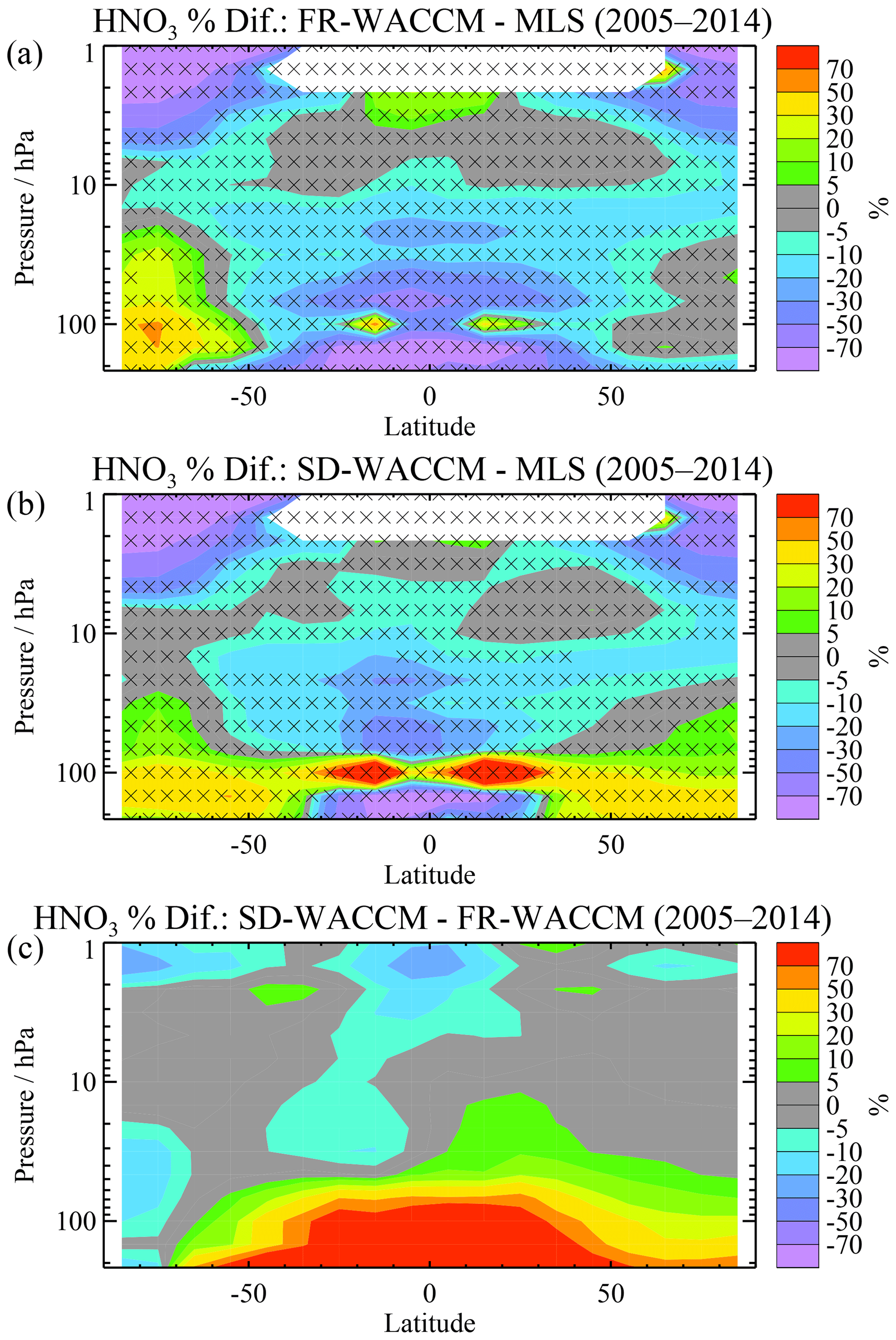
Finally, the comparisons for HNO3 (Fig. 6) reveal very few areas of model–data disagreements outside the systematic uncertainties. However, there is a model underestimation by both WACCM versions, especially in the polar upper stratosphere; this will be discussed more later. At high latitudes in the lower stratosphere, the models tend to overestimate the data. The upper troposphere is where the satellite-based HNO3 data have been validated the least, but there is some evidence for a high MLS bias in this region (see SPARC, 2017). While this might explain, qualitatively, why the models underestimate MLS tropical UT HNO3 (in Fig. 6), more work is needed to better evaluate HNO3 from models and satellite-derived data in this particular region.
It is also worth emphasizing differences between modeled and observed seasonal changes in the polar lower stratosphere over Antarctica. Indeed, we see in Fig. 7 that model HCl values at 46 hPa for 70–80∘ S do not decline as fast in early winter as shown in the data, even though SD-WACCM tracks the interannual variability better than FR-WACCM does (see Fig. S4 for the relevant time series). Uncertainties regarding lower-stratospheric heterogeneous chemistry modeling for SD-WACCM at high latitudes in the polar winter and spring have been discussed by Solomon et al. (2015) for one specific year (2011), including most of the features shown in Fig. 7. For our broader period, we see that the average rate of HCl decline from May to July (dominated by nighttime conditions) is slower in both SD-WACCM and FR-WACCM than the corresponding mean HCl rate of change from MLS (Fig. 7a). Grooß et al. (2018) recently discussed this HCl model–data discrepancy for dark polar vortex conditions, in comparison to simulations using the Chemical Lagrangian Model of the Stratosphere (CLAMS), which shows even larger HCl discrepancies. These authors discuss possible mechanisms and uncertainties, and they argue that additional decomposition of condensed-phase HNO3 might play a role, possibly via galactic cosmic ray impacts. Since this rapid decline in HCl occurs during polar night, this HCl issue does not lead to much difference in polar ozone loss rates, which only become significant during sunlit conditions (early spring). Figure 7 confirms that, on average, the SD-WACCM O3 decline and rise match the data well. We also note that FR-WACCM shows smaller-than-observed declines in HNO3 and H2O, whereas SD-WACCM matches these observations much better. The temperature panel (Fig. 7e) gives a possible reason for these differences, as T from FR-WACCM is larger by a few degrees during the coldest phase than T from SD-WACCM (MERRA-based) and larger than the MLS-derived values. This would lead to less irreversible denitrification and dehydration. The nature of the Fig. 7 results is similar at other lower-stratospheric pressures, although there is some variability in the magnitude of the differences. Over the Arctic region (not shown here), temperature-related differences are not as large as over Antarctica, but similar model–data differences in the early winter rate of HCl decline exist there also (as mentioned by Grooß et al., 2018).

Figure 7Each of the panels shows average seasonal changes from 2005 to 2014 for the 70–80∘ S region at 46 hPa. Data values (black) are from Aura MLS and model comparisons (FR-WACCM in blue, SD-WACCM in red) are provided for HCl (a), HNO3 (b), H2O (c), O3 (d), temperature (e), and N2O (f). For each month, the error bars represent twice the standard errors in the means, based on the set of 10-monthly averages (from 2005 through 2014).
As an addendum regarding the evaluation of models in comparison to data sets, we provide in Appendix A1 the results of a model grading approach used before (e.g., Douglass et al., 1999; Waugh and Eyring, 2008). We find that this grading method often leads to low grades (see Fig. A1), if applied using systematic uncertainty estimates from the MLS team (Livesey et al., 2018). The model results, as good as they are in many respects, cannot always match the data closely enough, at least based on such grades, although this grading formulation can be reconsidered or slightly modified. For example, the multiplicative error factor (see Eq. A1) can be increased (from 2 to 4) to force these grades to span a more useful range (see Fig. A2); some similarities to the percent difference diagnostics used here are noted in Appendix A1.
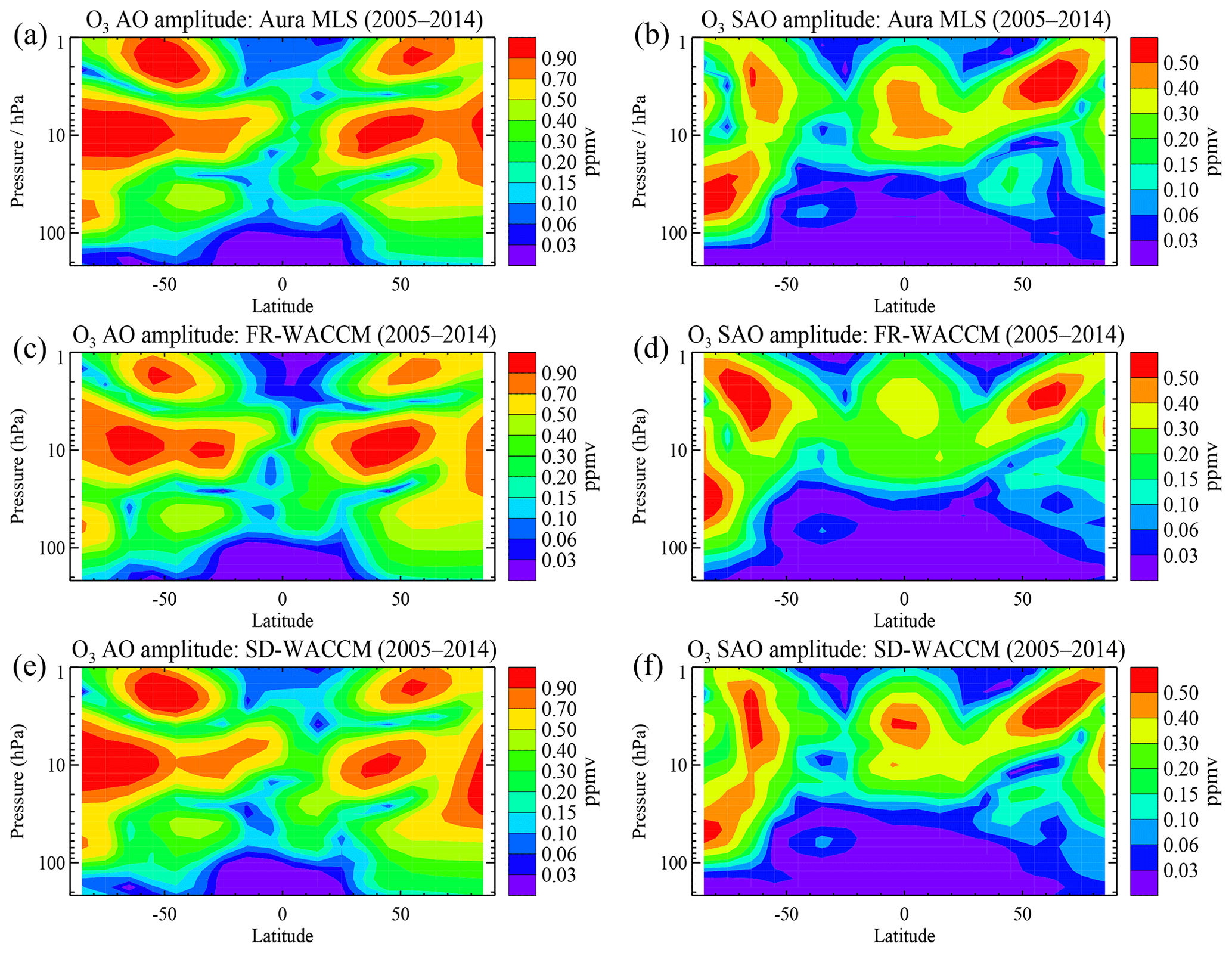
Figure 8Amplitude of the stratospheric ozone annual cycle (a, c, e) and semiannual cycle (b, d, f) for Aura MLS (a, b), FR-WACCM (c, d), and SD-WACCM (e, f), based on fits to time series from 2005 through 2014.
4.2 Annual and semiannual cycles
Figure 8 displays the amplitudes of annual and semiannual variations for MLS O3 and WACCM runs for 2005–2014. These results come from a simple regression fit to the monthly mean series in each latitude–pressure bin. The primary time dependence of the fitted function is given by additive sine and cosine terms (with 12-month and 6-month periods), in addition to constant and linear trend terms; the AO and SAO amplitudes are given by the square root of the sum of the squares of the corresponding fitted coefficients. We see from Fig. 8 that the overall data and model patterns of AO and SAO variability are quite similar. The O3 AO amplitudes peak at mid- to upper-stratospheric levels, with high-latitude variations also observed as a result of the effects of winter and spring polar chemistry and dynamics. The lower-stratospheric peak AO amplitudes are more prominent over the southern polar regions, where stronger O3 depletion occurs on a seasonal basis. These MLS O3 AO patterns are similar to those obtained by Schoeberl et al. (2008), using a much shorter period (September 2004 to December 2006); the same holds for other species (H2O and HCl). The observed SAO amplitude for O3 exhibits strong peaks in the upper stratosphere, both in the tropics and at high latitudes. The anti-correlation between O3 and temperature as a result of temperature-dependent photochemical production and loss terms for O3 has long been known to cause most of the O3 variability in the upper stratosphere (Perliski et al., 1989). The AO and SAO amplitudes obtained in that and other past studies (e.g., Ray et al., 1994) are similar to the patterns shown here. If we look more closely (and based on AO amplitude ratio plots not shown here), there are often O3 AO amplitudes 20 %–80 % larger than those derived from MLS data for both WACCM runs in the lower stratosphere (from 50 hPa at low latitudes to 215 hPa at high latitudes). Such model overestimates of the AO amplitude were shown in Fig. 2. Outside of this region, we observe somewhat closer fits to the MLS AO amplitudes for the SD-WACCM version, and both models track the data and each other well, with AO amplitudes typically within a range of ∼25 %. For the Antarctic lower stratosphere, the timing and magnitude of the seasonal recovery after the ozone hole plays a role, and we have observed that SD-WACCM generally fits the MLS data better than FR-WACCM does. In the tropical upper stratosphere, where the SAO is larger than the AO (see Fig. 8), the SD-WACCM results match the observed SAO amplitudes slightly better than those from FR-WACCM. Despite the existence of a few model–data differences, these AO and SAO amplitude comparisons, coupled with our examination of model/data amplitude ratio plots as well as the time series (which include the phase information), do not elicit major concerns regarding the model characterization of the primary processes expected to govern these modes of O3 variability. The study of dynamical forcing mechanisms in relation to such modes continues to be an active area of research (for example see Ern et al., 2015; Smith et al., 2017).
For H2O, a similar overview of the AO and SAO amplitudes is given in Fig. 9, which covers the range from 100 to 0.01 hPa. A peak in these amplitudes resulting from seasonal downward transport before the winter, followed by wintertime dehydration, is observed in the lower-stratospheric southern polar region; we note that SD-WACCM results match this feature better than FR-WACCM does. Other features include the Southern Hemisphere's upper-stratospheric AO peak in the extra-tropics. This has been seen by many satellite measurements (see Lossow et al., 2017a). Lossow et al. (2017b) explained this “island” feature in more detail; they argue that vertical advection tied to the upper branch of the Brewer–Dobson circulation largely explains the seasonal highs (lows) via downwelling (upwelling). They also show that an AO maximum is observed as well in other species in roughly the same region, including in N2O MIPAS (Michelson Interferometer for Passive Atmospheric Sounding) data. We confirm this behavior (see also Fig. S5) from the N2O AO amplitude feature observed in MLS data, as well as in the model runs (and more so in SD-WACCM). The derived AO and SAO amplitude patterns in H2O from Lossow et al. (2017a) are consistent with what we find; this includes the peak values in the upper stratosphere and mesosphere, attributed to combined effects of photochemistry and vertical transport. For ozone, a dominant feature in the SAO amplitude exists in the tropical upper stratosphere; see Lossow et al. (2017a) for a brief review of past work explaining such dynamically driven features for H2O. While there is generally a good level of model–data agreement in the main H2O AO and SAO patterns, both WACCM comparisons tend to underestimate observed AO and SAO amplitudes in the lower stratosphere and overestimate AO amplitudes in the SH mesosphere, while slightly underestimating mesospheric SAO amplitudes in both polar regions. The largest amplitude differences reach a factor of 2, in places, for the lower-stratospheric model underestimates; however, we note that this is also the region where AO and SAO amplitudes are smallest (typically <0.1 ppmv).
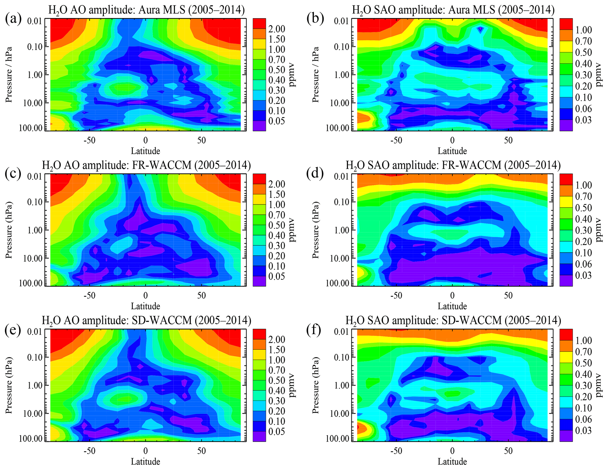
Figure 9Same as Fig. 8 but for H2O annual and semiannual cycles in the stratosphere and mesosphere.
For N2O, we already mentioned the existence of the upper-stratospheric AO peak (the “island” feature described by Lossow et al., 2017b) in the southern hemispheric extratropical region. This is similar to the H2O AO amplitude maximum feature, but the N2O seasonal variations are anti-correlated with H2O, as demonstrated by Lossow et al. (2017b), using MIPAS data (and as is also apparent in MLS time series, not shown here). Furthermore, we observe in Fig. S5 a somewhat better match in the AO and SAO N2O amplitude patterns for SD-WACCM than for FR-WACCM versus MLS, in particular for tropical to southern midlatitudes. This is also manifested in better time series fits for SD-WACCM, besides the closer match in average values; this is what one would generally expect from these two model versions. For HCl and HNO3, the AO and SAO amplitudes are dominated by the variations at high latitudes (see Figs. S6 and S7). The model HCl upper-stratospheric AO and SAO amplitudes match up fairly well with the observed amplitudes, despite the aforementioned issues relating to MLS upper-stratospheric HCl trends. For HNO3, the main AO and SAO model features follow the MLS patterns, although there is a model underestimation of the amplitudes in the upper-stratospheric polar regions, because these models do not properly capture the observed recurrences of enhanced HNO3, as mentioned earlier (see also Sect. 5).
5.1 Anomaly time series: fits and variability
5.1.1 Fits
We wish to evaluate which of the two WACCM models provides a better match, or fit, to the temporal variations in observed deseasonalized anomalies. We would expect SD-WACCM to generally fit these anomalies better than FR-WACCM. We calculate a diagnostic of model fit to the data by using the rms differences between these deseasonalized model and data series and normalize by dividing this quantity by the rms of the data anomalies themselves. A diagnostic value much less than unity means that the match to the series is much smaller than the typical variability; this also implies a good fit to observed anomalies. In Appendix A2, we provide the mathematical expression for this “rms difference diagnostic”. A better model fit to the observations will be given by a smaller rms difference diagnostic value. We also calculate the (Pearson) correlation coefficients, R, between model and data anomalies, and we use R2 as another measure of goodness of fit for the models. The first diagnostic is unitless and does not depart too much from the 0 to 1 range; R2 is limited to the 0 to 1 range, with larger values indicating a higher degree of linear correlation. We also use these two diagnostics together, by calculating the ratio of R2 over the rms difference diagnostic to obtain a “combined diagnostic”. This diagnostic could have a large value (a good model result) from both a large R2 in the numerator, meaning a high correlation with observed anomalies, and a small rms difference in the denominator, implying a good fit. This tends to amplify differences between two model comparisons to the same data. An ideal model fit would correlate tightly in time to observed oscillations but also exhibit the right magnitude by “hugging” the anomaly series. Indeed, two model series could have oscillations in phase with data variations and the same R2 values, but with different amplitudes and overall fits; conversely, two model series could have different R2 values versus observations, if one is more out of phase than the other, but they could still produce similar rms difference fits.
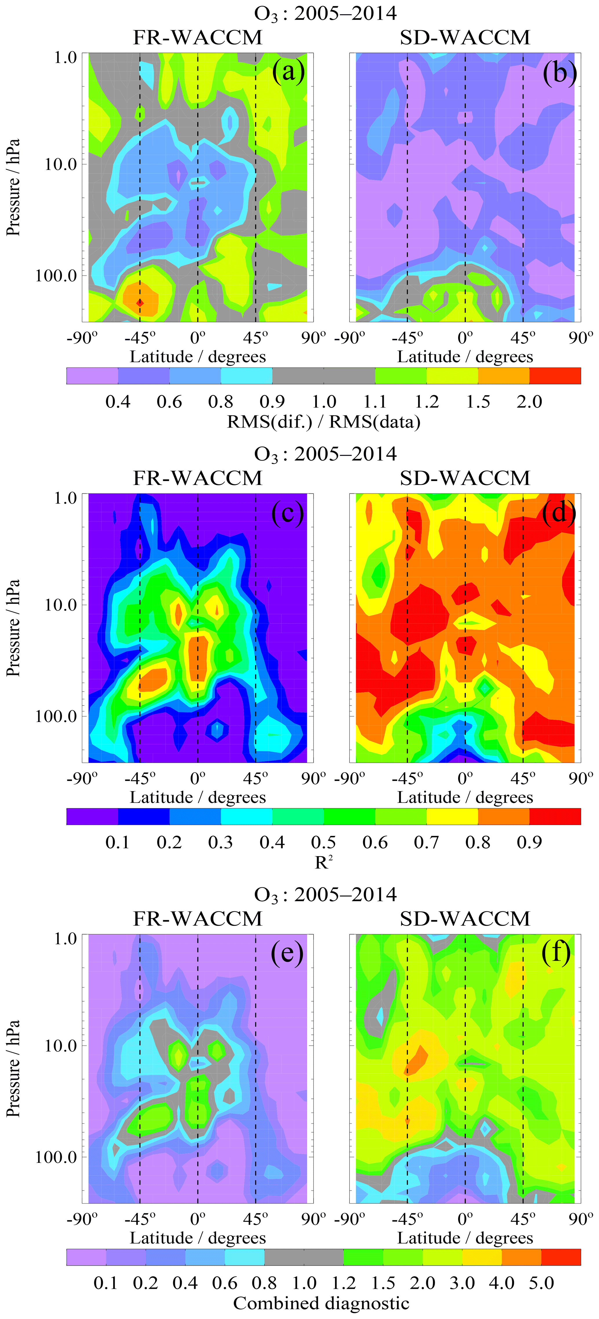
Figure 10Latitude–pressure contours of diagnostics that show how well the deseasonalized anomalies of model ozone time series (FR-WACCM, a, c, e; SD-WACCM, b, d, f) compare to MLS O3 anomaly series for 2005–2014. (a, b) show the rms difference diagnostic (see text) and (c, d) show R2 values; small rms difference values represent a closer fit, while large R2 values represent highly correlated results. (e, f) provide a combined diagnostic, namely the ratio of R2 to the rms difference diagnostic from the top panels; larger values here represent a better result for comparisons to the observed time series.
Figure 10 shows latitude–pressure contours of the above diagnostics for FR-WACCM and SD-WACCM O3 anomalies in relation to MLS anomalies for 2005–2014. We see from Fig. 10a and b that SD-WACCM rms difference diagnostic values (in the 0.2 to 1 range in the stratosphere) are smaller than those from FR-WACCM (between about 0.8 and 1.2). R2 values, between about 0.7 and 0.95 in most of the stratosphere, show that SD-WACCM correlates very well with the observations; R2 is somewhat smaller in the UTLS. The FR-WACCM O3 series correlate well with the data at low to midlatitudes for pressure levels between 70 and 7 hPa, which is also where the FR-WACCM rms difference diagnostic shows better performance and (as an explanation) where the dynamics are nudged (to tropical winds) in a similar way as for SD-WACCM. However, FR-WACCM shows almost zero correlation at high latitudes and in all of the uppermost stratosphere.

Figure 11Time series of monthly zonal mean O3 mixing ratios at 2.2 hPa (a, b) and deseasonalized anomalies (c, d), with the 0–10∘ N and 40–50∘ N latitude bins on the left and right, respectively. The two model time series (FR-WACCM in blue and SD-WACCM in red) are compared to the MLS series (in black) for 2005–2014. Diagnostic values (see text for a description) are shown in parentheses in the bottom two panels (c, d), with the first number referring to FR-WACCM and the second number to SD-WACCM.
Figure 11 shows sample O3 series for the upper stratosphere (at 2.2 hPa) for 0–10∘ N as well as 40–50∘ N. Although the tropical series show good correlations for both models versus data, some of the details in the observed semiannual peaks and the interplay between the AO, SAO, and the quasi-biennial oscillation are better followed by the SD-WACCM curve. The differences in O3 amplitude and phase are more clearly displayed in Fig. 11c, showing deseasonalized anomalies. Diagnostic values provided in this panel show that SD-WACCM performs better than FR-WACCM, with a much larger R2 value and a smaller rms difference diagnostic value and, hence, a much better combined diagnostic value. The same comments apply to Fig. 11b and d, which showcase the NH midlatitudes at 2.2 hPa. In the high-latitude lower stratosphere, the poorer FR-WACCM results in Fig. 10 are generally caused by time series that are less in phase with polar winter and spring variations, as well as by more departures in variation magnitudes. Figure 10e and f amplify model differences, with combined diagnostic values mostly below 1 for FR-WACCM but between 1 and 3 in the SD-WACCM case. The more realistic dynamics in SD-WACCM allow for better SD-WACCM fits, as shown in Figs. 10 and 11. These plots also point to poor upper tropospheric results for both models (with SD-WACCM slightly better), although this is not the focus of this paper.
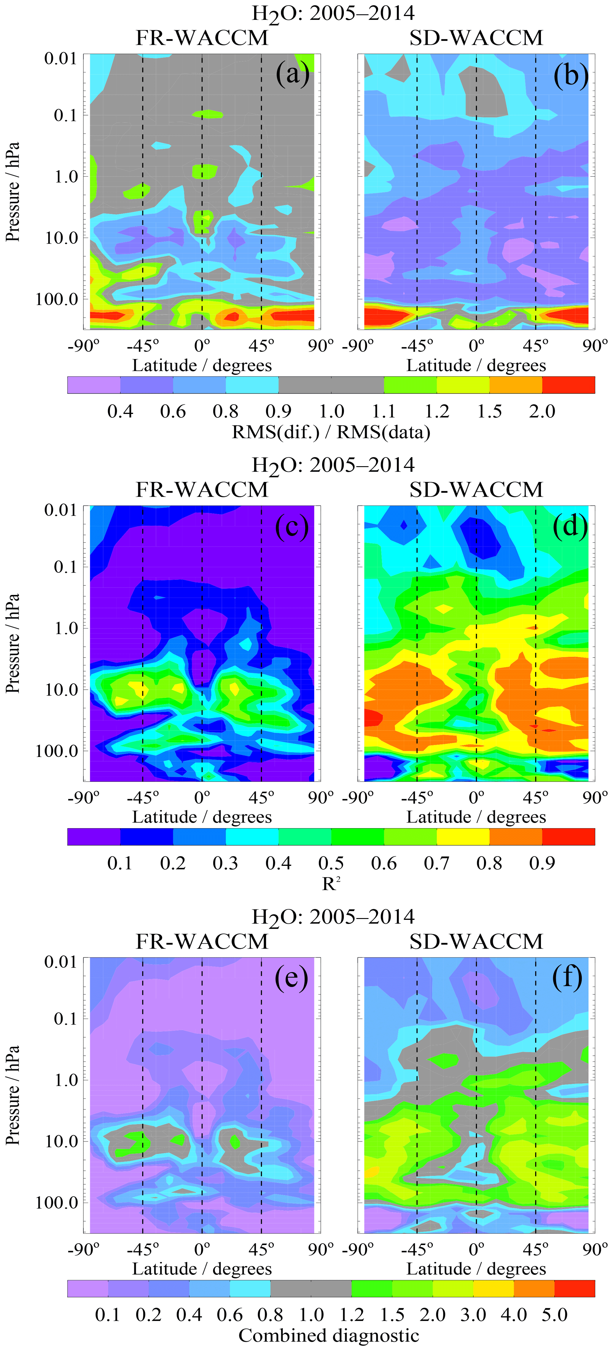
Figure 12 describes the same diagnostics as above but for model–data H2O comparisons and a top level at 0.01 hPa. Again, the diagnostics of fit are usually much better for SD-WACCM, which yields R2 values of 0.6 to 0.9 and rms difference diagnostic values below 1 for most of the stratosphere and lower mesosphere, and therefore better combined diagnostic results than FR-WACCM. The SD-WACCM diagnostics are poorest in the upper mesosphere and at high latitudes near 215 hPa. In the upper stratosphere and mesosphere, the better diagnostic results for SD-WACCM are seen in time series (not shown) as a better match versus the MLS H2O anomalies in terms of the interannual variability at all latitudes, as well as for some seasonal peaks at high latitudes. We interpret this as the result of a better dynamical representation of the mesosphere for SD-WACCM. The high-quality representation of mesospheric composition by SD-WACCM is also demonstrated in comparisons to measurements of CO profiles above Kiruna, Sweden, by MLS and the Kiruna Microwave Radiometer (Ryan et al., 2018). For H2O near 200 hPa, poor fits at high latitudes occur where MLS data exhibit a dry bias versus sonde and Atmospheric Infrared Sounder (AIRS) data, as discussed in MLS data documentation (Livesey et al., 2018), as well as by Vömel et al. (2007) and Davis et al. (2016). MLS H2O is low by a factor of several here versus the WACCM runs (which show values of 10–60 ppmv). The data variability may also be affected by the dry bias retrieval (and oscillation) issues at the lowest altitudes at high latitudes, where observed anomalies are more poorly tracked by the models; a planned future update to the MLS H2O retrievals will help to mitigate this discrepancy.
Figure S8 displays results similar to Fig. 10 but for stratospheric HCl. SD-WACCM HCl results versus MLS are superior to those from FR-WACCM and show high correlations (R2>0.7) in most of the lower stratosphere, with somewhat poorer results in the upper stratosphere, where the rms difference fits and the combined diagnostic are poor for both models. This upper-stratospheric issue is caused by a data problem in this region, where MLS HCl trends are known to be too flat (close to zero). Poorer correlations are observed for FR-WACCM at high latitudes, but even subtle differences in the timing (phase) can lead to poorer correlations. Poorer fits at 100 hPa in the deep tropics are related to a large underestimate of the data, which may be caused, in part, by a high bias from MLS (Froidevaux et al., 2008b) but more so, for R2, by out-of-phase model variability.
For N2O, we also observe in Fig. S9 (showing model comparisons to the 68 to 1 hPa observations from the 190 GHz MLS N2O band for 2005–2014) that SD-WACCM fits the data better than FR-WACCM, in both the R2 and the rms difference categories. FR-WACCM exhibits poor results in the upper stratosphere and at high latitudes in the lower stratosphere. Both models exhibit poorer rms fits and poorer correlations in the tropical lower stratosphere. Partly, this appears to be caused by a model underestimation of the MLS N2O variability in this region, with some QBO phasing differences as well.

Figure 13HNO3 monthly zonal mean mixing ratio time series (2005 through 2014) from MLS, FR-WACCM, and SD-WACCM for 3.2 hPa and 70–80∘ S.
HNO3 results (see Fig. S10) show, again, better fits to stratospheric MLS data from SD-WACCM than from FR-WACCM and poor performance from FR-WACCM at high latitudes. Both models do poorly in the upper stratosphere, and Fig. 13 illustrates the magnitude of this discrepancy in the region (3.2 hPa and 70–80∘ S) where it reaches its maximum. Since its launch, MLS has been observing very large values of HNO3 in the upper stratosphere, mostly in the polar regions during winter. The WACCM runs used here do not include the necessary photochemical pathways, including the effects of energetic particle precipitation on ion chemistry in the upper atmosphere, to adequately represent such variations; implementation of the necessary missing chemical reactions has not made its way into most CCMs. The solution seems tied to ion cluster chemistry during energetic particle precipitation (EPP) events, which includes large solar proton events (SPEs) as well as more regular auroral activity. Direct high-altitude EPP effects enhance NOx, which can propagate downward in polar winter and increase stratospheric NOx and HNO3 via this indirect effect and conversion of N2O5 on ion water clusters (Böhringer et al., 1983). Large polar enhancements in upper-stratospheric HNO3 were observed by the MIPAS after SPE activity in 2003 (Orsolini et al., 2005; von Clarmann et al., 2005; Lopez-Puertas et al., 2005; Stiller et al., 2005). More complex modeling (e.g., Funke et al., 2011; Verronen et al., 2011; Kvissel et al., 2012; Andersson et al., 2016) has produced EPP-induced enhancements in high-latitude HNO3, with related improvements in model–data comparisons into the mesosphere. Regarding low-latitude upper-stratospheric HNO3, the poorer model fits seem to be caused at least in part by more noisy and variable MLS data, under low HNO3 conditions. Finally, tropical MLS HNO3 data at 147 and 215 hPa are not fit well by either model, as the data exhibit seasonal oscillations between 0.2 and 0.5 ppbv, whereas model values are smaller than 0.1 ppbv. There have been few tropical UT validation comparisons for HNO3 (Santee et al., 2007), but in situ data from an airborne chemical ionization mass spectrometer have shown that UT HNO3 tropical values are mostly below 0.1–0.2 ppbv (Popp et al., 2007, 2009).
We saw in Sect. 4 that there are good climatological comparisons between SD-WACCM and MLS variations over Antarctica during polar winter and spring, except for the rate of HCl decline in early winter; also, poorer results are obtained by FR-WACCM. We also find, not too surprisingly, that interannual differences in lower-stratospheric chemical evolution over Antarctica are not as faithfully reproduced by FR-WACCM as by SD-WACCM. This is shown by the anomaly time series comparisons of Fig. S11 for O3 and temperature at 68 hPa and 70–80∘ S, along with the associated model diagnostic values. These plots also show that springtime anomalies dominate the variability, with warmer-than-usual springs (in October in particular), such as in 2012 and 2013, leading to more positive ozone anomalies, i.e., less ozone depletion; conversely, years (2006, 2008, 2010, 2011) with colder-than-usual springs are correlated with negative ozone anomalies and more depleted conditions.
5.1.2 Variability
Given our expectations that SD-WACCM would match observed time series of multiple species better than FR-WACCM, and having demonstrated this in the previous section, we turn to what should be a more fair comparison between the two sets of model results, namely the variability aspect. We calculate the ratio of model to data interannual variability, as obtained from the root mean square values of deseasonalized monthly anomaly series, expressed as a percent of climatological means; a simple linear trend is first subtracted from the series, so that the variability comparisons remove any significant trend differences. We do this for the MLS data, but also for longer-term time series, using the GOZCARDS data. The models are sampled following the monthly sampling of the data sets (but not at the daily sampling level of detail); sampling plays a role for the longer-term (merged) GOZCARDS data, which are comprised of some unevenly sampled occultation data records (depending on latitude and pressure). Figure 14 compares the O3 variability ratios (models versus data) using as a reference the MLS 2005–2014 data (Fig. 14a and b) and the GOZCARDS merged ozone (1992–2003) data (Fig. 14c and d). To first order, we observe similar patterns for both time periods. The SD-WACCM variability is generally within 10 %–20 % of the data variability (ratio values between 0.8 and 1.2). The FR-WACCM variability is somewhat smaller than the data variability in the polar regions and in the upper stratosphere. Bandoro et al. (2018) also found that the free-running version of WACCM displays smaller ozone variability in the upper stratosphere, both for shorter-term and longer-term variabilities, than the observed variability, based on the merged SWOOSH O3 data record. In the lower stratosphere at low to midlatitudes, FR-WACCM exhibits slightly larger variability than the data, whereas SD-WACCM shows slightly smaller variability than the data; Bandoro et al. (2018) found that FR-WACCM slightly overestimates the decadal variability in this region. We also see in Fig. 14 that, at high latitudes, FR-WACCM underestimates the actual variability, whereas this is less of an issue for SD-WACCM, with its more realistic representation of the dynamics; as an example, refer to Fig. 13 for model and data anomalies at 68 hPa and 70–80∘ S.
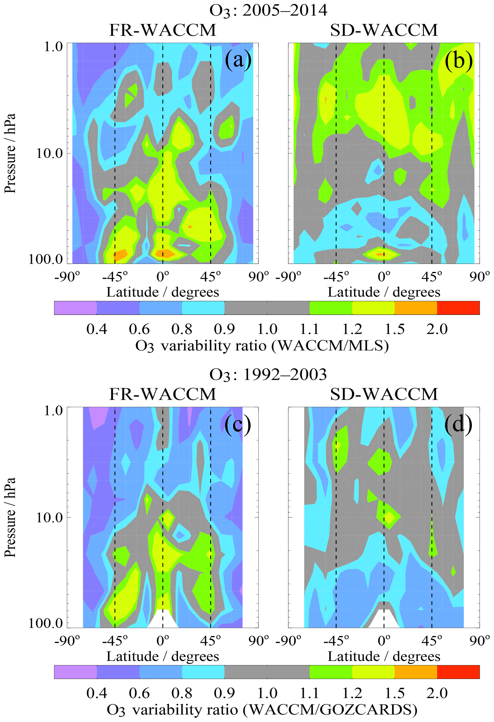
Figure 14Variability ratios (model results divided by data results) for stratospheric O3, with FR-WACCM results on the left (a, c) and SD-WACCM on the right (b, d). Before calculating the ratios, the variability values are obtained as the root mean square of detrended deseasonalized monthly anomaly time series and expressed as a percentage of mean (climatological) abundances; (a, b) show comparisons to MLS data for 2005–2014, whereas (c, d) are for 1992–2003 comparisons to GOZCARDS.
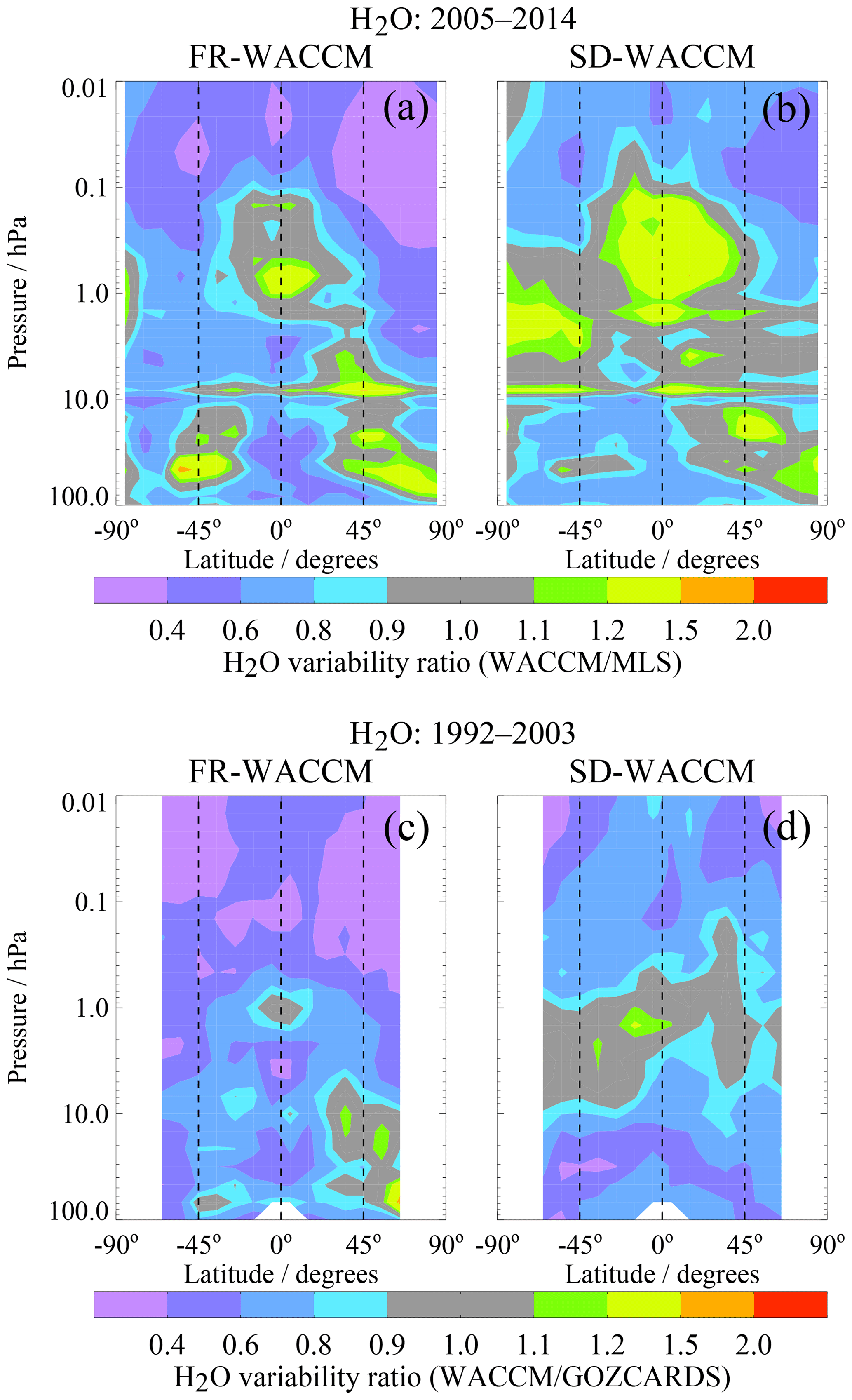
Figure 15Same as Fig. 14 but for ratios (model/data) of H2O stratospheric and mesospheric variability for two different time periods.

Figure 16Time series (1992–2014) at 100 hPa and 10–20∘ S for temperature (b, d) and H2O (a, c), with deseasonalized anomalies shown in (c, d). The temperature plots just show the two models (FR-WACCM in blue, SD-WACCM in red), whereas the H2O series show the comparisons for the models versus GOZCARDS merged H2O data (in black).
A similar overview of model/data variability ratios is provided for H2O in Fig. 15, for the mesosphere and the stratosphere. Here, while the variability from SD-WACCM is closer than that from FR-WACCM to the data variability during both periods, the tendency for both models is to underestimate the observed variability, with FR-WACCM showing a stronger underestimate in the upper stratosphere and mesosphere. Such an underestimate for FR-WACCM implies that a trend detection in the future will require more years of data, if H2O continues to have larger variability than models. The FR-WACCM underestimate of the variability is sometimes by as much as a factor of 2, although it is more typically by ∼30 % (see Fig. 15). For a series with rms variability about the fit represented by σt, the number of years needed to statistically detect a trend is proportional to (Weatherhead et al., 1998), and thus an increase of σt by factors of 1.3, 1.5, and 2.0, for example, will lead to an increase in the number of years for trend detection by factors close to 1.2, 1.3, and 1.6, respectively. In the tropical lower-stratospheric case, H2O and temperature values and anomalies for 1992–2014 are shown for 100 hPa and 10–20∘ S in Fig. 16. Again, we note the smaller-than-observed variability in model H2O oscillations, with SD-WACCM tracking the data better. This correlates with the temperature series, where smaller variability is seen in FR-WACCM, in comparison to SD-WACCM (which follows MERRA temperatures); we also note that FR-WACCM temperatures are somewhat larger (by ∼1 K on average) than SD-WACCM temperatures in this region. This poorer tracking of cold point temperatures for FR-WACCM (Fig. 16) has likely implications for poorer stratospheric trend results for FR-WACCM H2O as well, as we will actually observe in the trends section (Sect. 5.2). It is well known that stratospheric entry level H2O is governed by temperatures near the tropopause cold trap; the monthly average variations shown here are similar to what has been shown in past H2O work (e.g., Randel et al., 2004, 2006; Randel and Jensen, 2013). Brinkop et al. (2016) used model runs from both free-running and nudged simulations to analyze the impacts of different constraints, including sea surface temperatures (SSTs) and meteorological fields, on sudden drops in H2O; they found that several of these factors play a role in the H2O variations, including the timing of El Niño–Southern Oscillation (ENSO) and SST variability, the phasing with the QBO, cold point temperatures, and the correct dynamical model state. Many other analyses of the relation between entry level H2O, tropopause temperatures, transport, and convection have been carried out previously (e.g., Holton and Gettelman, 2001; Jensen and Pfister, 2004; Fueglistaler and Haynes, 2005; Rosenlof and Reid, 2008; Read et al., 2008; Schoeberl et al., 2013). Our point here is that the WACCM H2O anomaly series underestimate the observed variability. We note also that this model underestimate exists if we calculate relative variability using a maximum minus minimum range from yearly average anomalies rather than monthly averages. We provide a global view of lower-stratospheric variability differences (models versus data) in the anomaly series comparisons at 83 hPa for all latitude bins in Fig. S12. This also shows that the observed interannual changes in H2O are better followed by SD-WACCM than by FR-WACCM, including the drop in H2O after 2011 (see Urban et al., 2014). While lower-stratospheric H2O variability is underestimated by SD-WACCM by ∼20 %, the correlation between SD-WACCM and observed anomalies is very good (as was shown in Fig. 12).
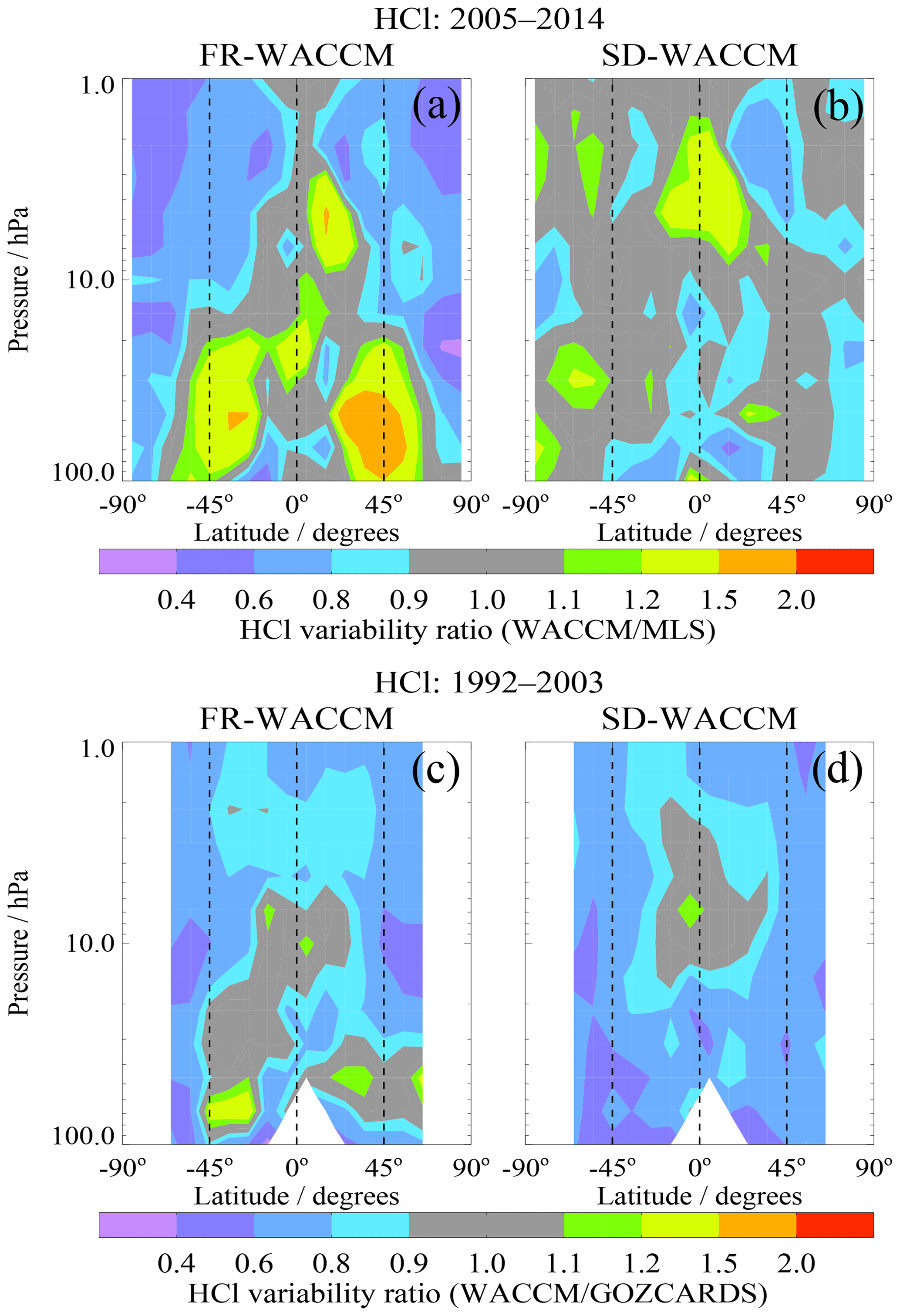
For HCl, we show the (detrended) variability ratios in Fig. 17. The observed HCl variability is fairly well matched (within ∼20 %) by both models in the MLS time period, with an edge given to SD-WACCM. The observed variability is often underestimated (by ∼30 %) by both FR-WACCM and SD-WACCM in the earlier period (1992–2003). We believe that the HALOE sampling plays a role in this; i.e., even if we limit the model comparison (as we do here) to just the same months as when HALOE observations occurred, incomplete sampling in latitude and time can lead to differences versus a fully sampled model (see Toohey et al., 2013) and more so in the polar regions where the HCl variability is large. In the upper stratosphere, the variability ratios are comparable to or somewhat smaller than those in the middle stratosphere, and there is a 20 %–30 % underestimate of the observed variability, which is based on HALOE HCl observations for 1992–2003. There have been difficulties in fully understanding (or modeling) observed upper-stratospheric HCl variations before the declining phase that started after about 2000 (Waugh et al., 2001); see also Sect. 5. For 2005–2014, SD-WACCM actually matches the upper-stratospheric MLS variability fairly well, although these variability values are small.
We also show the ratios of model to data variability for stratospheric HNO3 (2005–2014) and N2O (2005–2012) in Fig. S13. We already discussed the issues with missing model chemistry for upper-stratospheric HNO3 variability, as well as the low signal-to-noise issue for HNO3 data at low latitudes in this region. There is reasonably good agreement in the HNO3 variability between SD-WACCM and MLS for the lower to mid-stratosphere, while FR-WACCM generally overestimates the HNO3 variability in this region. Figure S13 shows N2O results down to 100 hPa. Here, MLS N2O–640 data (from the 640 GHz radiometer) for 2005–2012 are used; these retrievals were curtailed in the first half of 2013 as a result of degradation in the 640 GHz radiometer signal chain. Based on results shown in SPARC (2017), there appears to be good agreement in the tropical interannual variability comparisons for N2O at 100 hPa between MLS and other satellite-derived results. The lower-stratospheric N2O time series behave more smoothly at low latitudes in the models than in the observations. The interannual variability in the MLS N2O measurements there is somewhat smaller than the standard deviations in monthly mean N2O values (of 20–30 ppbv). The MLS N2O measurement noise itself for a monthly zonal mean (made up of about 5000–6000 profiles) should be less than 1 ppbv. Smoothing the model in the vertical domain to better match the MLS vertical resolution would not lead to a better fit to the observed variability. However, we should keep in mind that the MLS-derived N2O variability is a small percentage (<3 %) of the monthly zonal mean N2O abundances. In summary, SD-WACCM shows some underestimate of the observed lower-stratospheric tropical variability for all the species considered here, except for HNO3; FR-WACCM does so also for three species (H2O, HCl, and N2O). It may be that some of the larger variability in the measurements arises from effects not tied just to MLS radiance noise issues, or from variability caused by the proximity to the tropopause for measurements with finite vertical resolution; WACCM could also be genuinely underestimating the actual atmospheric variability near the tropopause (for unknown reasons).
5.2 Trends
In this section, we discuss how the WACCM runs compare to stratospheric observations when it comes to trends, from fairly short-term trends (from the Aura MLS time period) to longer-term trends based on comparisons with O3, H2O, and HCl GOZCARDS data records (see Sect. 2 and Froidevaux et al., 2015). Trend analyses have their own complexities in terms of analysis methods and uncertainty estimates. For example, O3 trend assessments have had to deal with trend estimates from different long-term data records, each with its own characteristics (Tummon et al., 2015; WMO, 2014; Harris et al., 2015; Steinbrecht et al., 2017; Ball et al., 2017, 2018). This kind of analysis is especially difficult when investigating trends from time series with high variability compared to the size of an underlying long-term change over time, which is certainly an issue for the lower stratosphere. Also, global modeling efforts have led to improved characterizations of the expected combined and separate impacts on ozone profiles of long-term changes in halogen source gases and greenhouse gases (WMO, 2014).
Here, we focus mostly on trend results from WACCM and observations, given the application of the same analysis methods for the different series. We have applied multiple (or multivariate) linear regression (MLR) to the time series of deseasonalized anomalies from the data, FR-WACCM, and SD-WACCM. In Appendix A3, we provide more details regarding the regression model, which includes commonly used additive functional terms, including constant, linear, and periodic terms, along with proxies describing well-known variations arising from the QBO and ENSO, as well as an 11-year solar cycle proxy term. Examples of observational time series from merged ozone observations for 1998 through 2014 are provided in Fig. A3, along with the fits to the series and the linear components (trends). We also discuss our methodology (a block bootstrap method) for trend error evaluations in Appendix A3; such an approach was used, for example, by Bourassa et al. (2014) for their trend analyses of ozone from the OSIRIS (Optical Spectrograph and Infrared Imager System) retrievals. We display the resulting trend error bars as 2σ values (which is very close to the 95 % bounds on the distribution of trend results). Such calculations often lead to significantly larger error bars than more standard methods or code (which neglect the autocorrelation of the residuals).
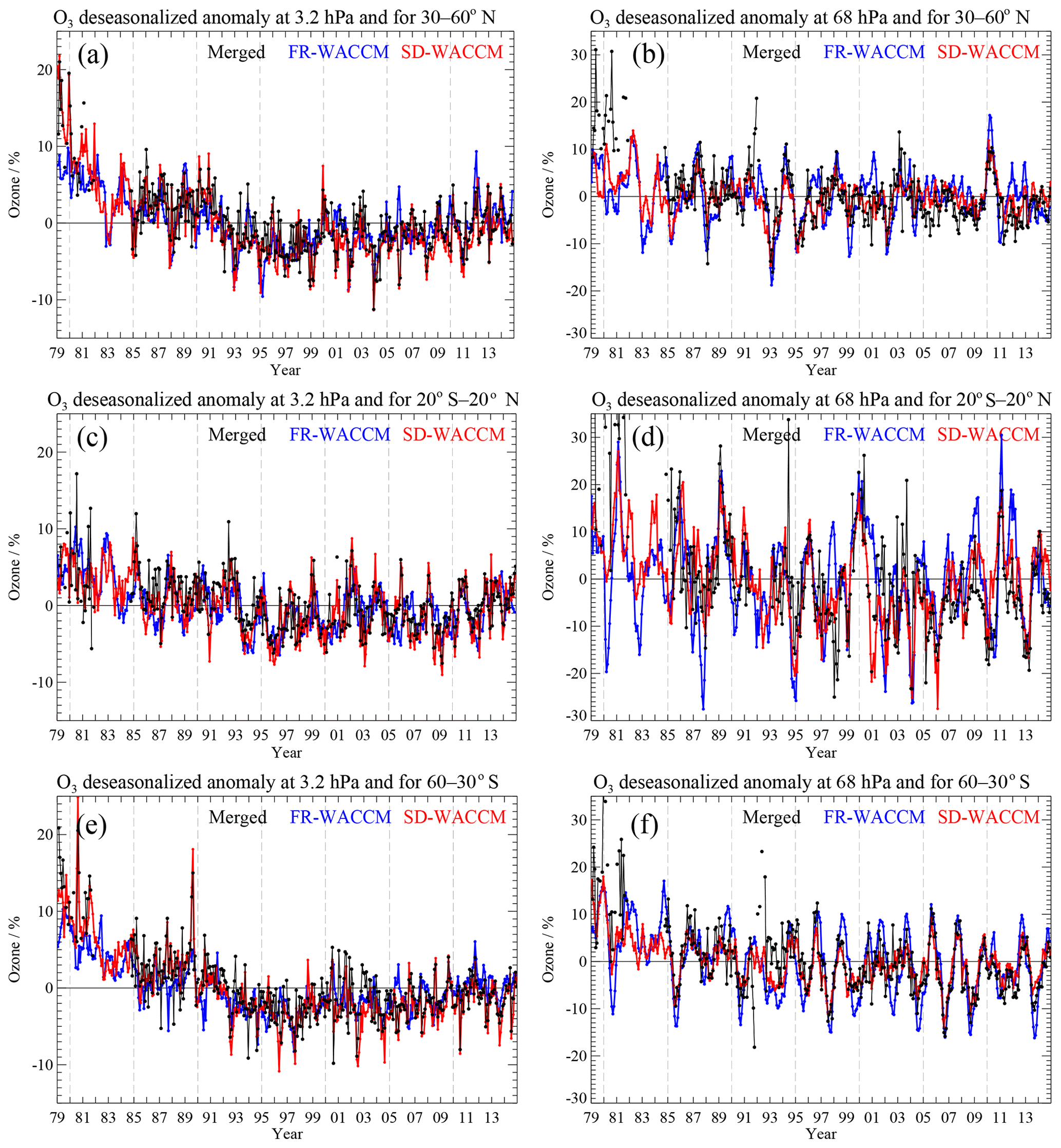
Figure 18Sample time series of deseasonalized ozone anomalies (%) from 1979 through 2014 from the GOZCARDS data record (version 2.20) compared to the corresponding model anomalies from FR-WACCM (blue) and SD-WACCM (red). Upper-stratospheric series at 3.2 hPa are shown in (a, c, e) and lower-stratospheric series at 68 hPa in (b, d, f); three latitude bins are displayed (30–60∘ N, a, b; 20∘ S–20∘ N, c, d; and 30–60∘ S, e, f).
For ozone, we give an overview in Fig. 18 of percent deseasonalized anomaly time series for three latitude bins (northern midlatitudes, tropics, and southern midlatitudes) and two pressure levels (3.2 hPa for upper stratosphere, 68 hPa for lower stratosphere). The series were deseasonalized in 10∘ latitude bins and then averaged. The GOZCARDS data used here (version 2.20) are an update to the original (version 1.01) record (Froidevaux et al., 2015), as mentioned in Sect. 2. Figure 18 shows generally good agreement between the various time series, although if one looks carefully, SD-WACCM is generally closer to the observational time series than FR-WACCM is, as one might expect from previous considerations of goodness of fit and variability; also, percent variability is larger in the lower stratosphere than in the upper stratosphere, thus rendering trend detection more difficult at lower altitudes. We compare in Fig. 19 the ozone profile trend results from MLS data alone, from 2005 through 2014, to those from FR-WACCM and SD-WACCM, for the three aforementioned latitude bins. We show the error bars as 2σ estimates, as this provides an easy way to visualize if there are significant differences between models and data, or between models. Furthermore, we have also shown (in grey) the data trend results for time series through the end of 2018, as a timely reference, but with no corresponding available model results. Trend results through 2018 also help to underscore how trend variability depends on the number of years used in the analyses. For ozone, this shows that there are certainly some altitude and latitude regions where the slightly longer-term trends differ from the shorter-term trends by as much as 0.2 % yr−1 (a typical 2σ uncertainty), and especially at northern midlatitudes in the lowest altitude region, where a significant decrease in trend values is obtained (from 0.5 to 0.9 % yr−1 to near zero for the longer-term trend). In contrast, the southern midlatitudes show that the longer-term trends are positive throughout the stratosphere, whereas slightly negative values were obtained for 2005–2014. These changes can be traced back to ozone variability in the observational record; this underscores that large dynamical variability in the lower stratosphere will continue to create significant variability in the trends. Indeed, the importance of meteorological variability was recently emphasized by Chipperfield et al. (2018), who included MLS data through the end of 2017 in their comparisons to simulations from a chemical transport model; they showed that the MLS data exhibited large increases in the SH lower stratosphere in 2017, which led to a positive tendency for 2005–2017 trends in that region, in contrast to slight declines (or near-zero trends) in the NH, in general agreement with the results shown here, which include one more year (2018) of MLS data. Moreover, Fig. 19 provides a robust indication from the MLS data alone that upper-stratospheric ozone values have been on the upswing in the past decade, at a rate of about 0.1 to 0.3 % yr−1, depending on latitude–altitude region, with 2σ uncertainties of ∼0.2 % yr−1. While these 2σ error bars (obtained using the bootstrap method mentioned earlier) are fairly large, there are several latitude regions and pressure levels with similar results, and this positive trend is a robust near-global upper-stratospheric result (with even smaller uncertainties). These results are broadly consistent with O3 trends obtained by Steinbrecht et al. (2017), who use MLS as part of the longer-term merged data records, although they studied a longer time period (2000–2016). All things being equal, the errors in these trends should diminish as more years of data are added to the MLS O3 record, which, for the middle and upper stratosphere, has been characterized as “very stable”, namely within 0.1 to 0.2 % yr−1 versus sonde and lidar network ozone data (Hubert et al., 2016); it seems difficult to quantify “absolute stability” to much better than this, especially in the lower stratosphere. In the lower stratosphere, trend results are closer to zero, with larger variability and error bars (in % yr−1), and unambiguous detection of post-1997 ozone trends in this region remains elusive (WMO, 2014; Harris et al., 2015). The 2005–2014 trends in Fig. 19 show good broad agreement between model and data, with a tendency for SD-WACCM to agree better than FR-WACCM with MLS, albeit not significantly so, given the size of the error bars, especially in the lower stratosphere. The lower-stratospheric tropical results from FR-WACCM are negative, in contrast to both the observations and SD-WACCM, but with large error bars. In the tropical upper stratosphere, both models exhibit a somewhat more positive trend than observed for this period, with FR-WACCM diverging more from the observations than SD-WACCM does. We do find it rather striking that, as a function of latitude (in 10∘ wide bins) and pressure, the 2005–2014 SD-WACCM O3 trends follow the MLS trend results quite well; this is clearly shown in Fig. 20 for central latitudes from 55∘ S to 55∘ N. As mentioned above (but not shown in Fig. 20), the agreement in these patterns is not as good for FR-WACCM.
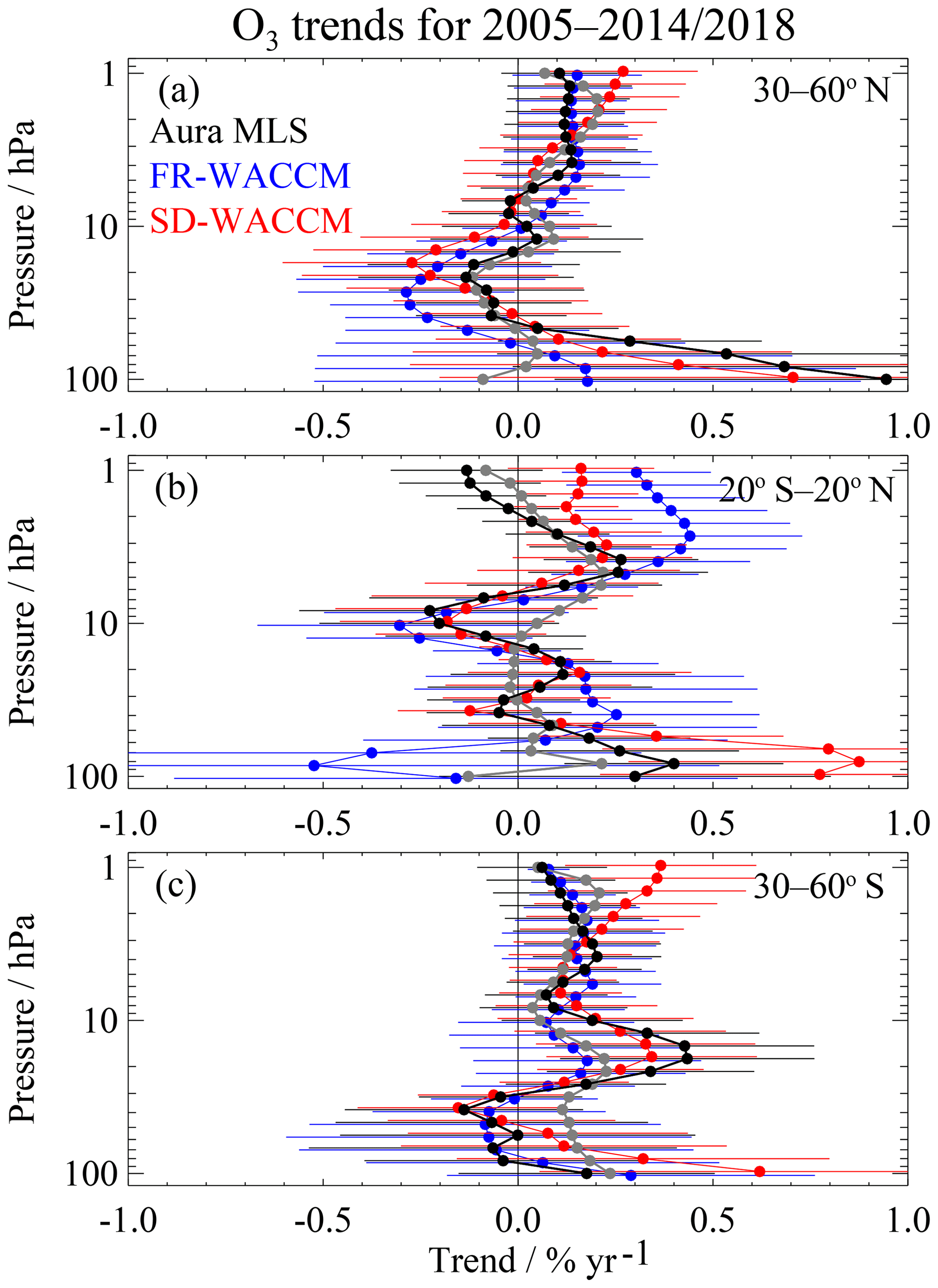
Figure 19Ozone stratospheric trends for 2005 through 2014 obtained from monthly zonal mean data (version 4.2 Aura MLS) and models (FR-WACCM and SD-WACCM), after multiple linear regression analyses of deseasonalized anomaly time series, as described in the text. Each panel refers to results from different latitude band average series (see legend). The error bars are 2σ estimates based on bootstrap resampling results (see text). We also show the data trends for 2005–2018 (in grey) to provide an update on how the past 4 years change the (slightly longer-term) tendencies; to avoid more clutter in these plots, we have not overplotted the corresponding error bars, but these are only slightly smaller than the black observational error bars.
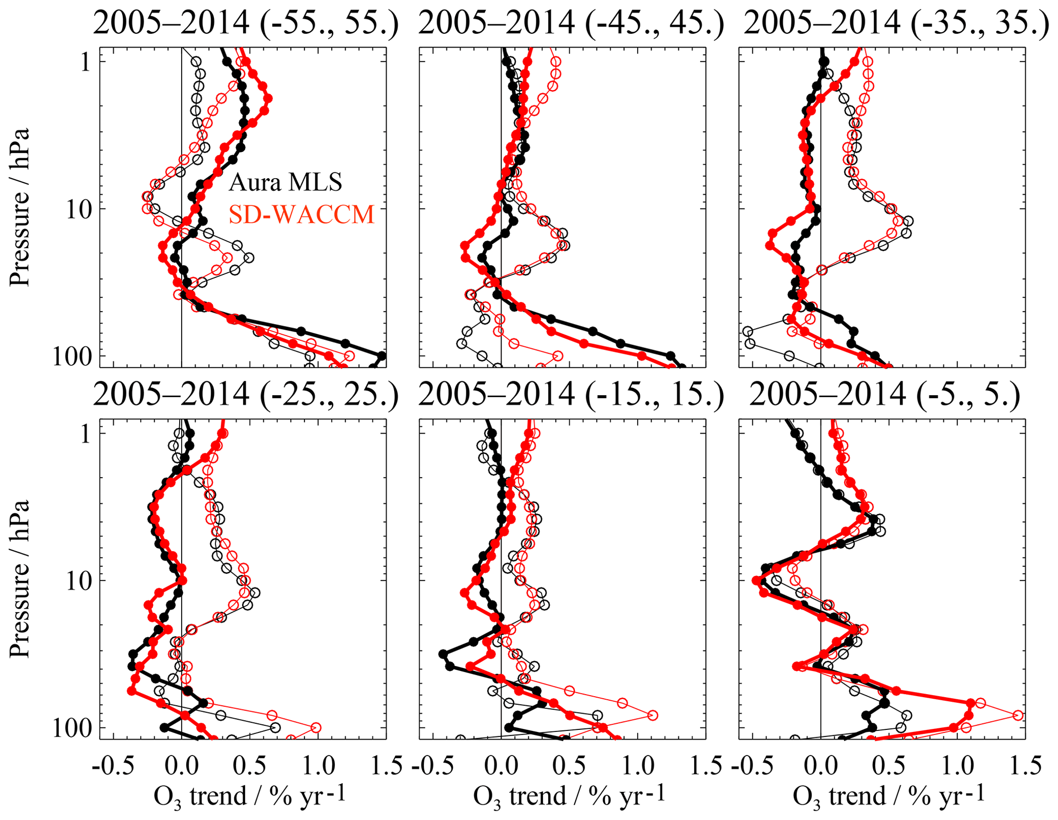
Figure 20Ozone trends in different latitude bins for SD-WACCM (red) versus Aura MLS data (black) for 2005–2014. Closed and open circles are for northern and southern latitude bins, respectively. For clarity, error bars are omitted here, as these generally show that model–data trend differences are not significant for this time period.
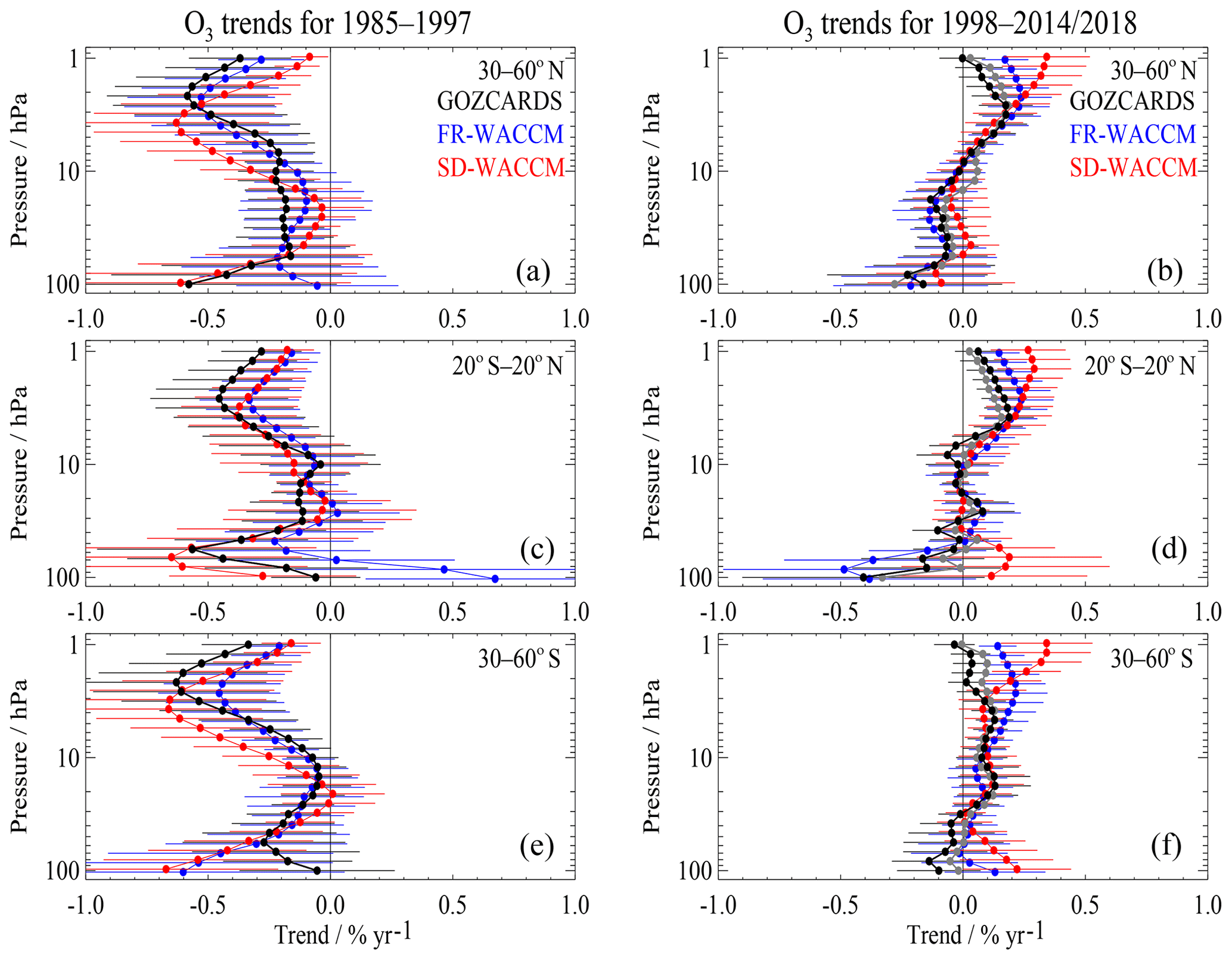
Figure 21Same as Fig. 19 for ozone trend comparisons, except for the use of longer-term GOZCARDS (version 2.20) ozone data records, with 1985–1997 shown in (a, c, e) and 1998–2014 in (b, d, f), along with the corresponding model results. We also show the updated ozone data trends with 1998–2018 results in grey (for b, d, f).
For a consideration of longer time periods, we compare in Fig. 21 trends from the merged O3 GOZCARDS record (version 2.20) to model results for two time periods: Fig. 21a, c, and e for 1985–1997 focus on the main declining ozone phase, while Fig. 21b, d, and f show the post-1998 early ozone recovery stages. The largest differences between the two GOZCARDS data versions occur in the tropical upper stratosphere for the declining ozone phase; Fig. S14 displays the tropical trend differences that we obtain for the same three periods as in Fig. 19. In agreement with this are the trend differences provided by Ball et al. (2017), who showed results for the original (version 1.01) GOZCARDS data and for SWOOSH. GOZCARDS version 2.20 data are now in better agreement with the merged SWOOSH O3 product (as both use SAGE II version 7 data); also, Steinbrecht et al. (2017) showed that these two merged records lead to similar (post-2000) trend results. The improvements in GOZCARDS version 2.20 ozone are a result of the incorporation of the SAGE II v7 retrievals (Damadeo et al., 2013) and the use of the MERRA temperatures (used in v7) for the conversion from density–altitude to the GOZCARDS mixing-ratio–pressure grid. We note, however, that the lower-stratospheric region exhibits interannual variability that is several times larger than that in the upper stratosphere, as seen in Fig. A3 for tropical 1998–2014 data versus SD-WACCM. Even fairly subtle differences in time series over a few years can lead to a sign change in the trends, although there is no statistical significance in the resulting trend differences. For the pre-1998 period, Fig. 21 shows generally good agreement in the trends versus the models; FR-WACCM tends to fit the observed trends more poorly than SD-WACCM in the lower stratosphere, although the upper-stratospheric results at midlatitudes are somewhat poorer for SD-WACCM. The longer-term trends for 1998–2018 based on GOZCARDS data show slightly more positive trends than the 1998–2014 results, and the recent ozone changes that affected the results in Fig. 19 (with a 2005 starting year) are diluted somewhat for the period starting in 1998. The Southern Hemisphere midlatitudes exhibit near-zero or slightly positive trends over the whole stratosphere, for 1998–2018; we note that zero trends are included inside the corresponding error bars, although we did not add (grey) data error bars in these (already busy) plots. We note also that the upper-stratospheric early recovery (positive trends) is robust in the GOZCARDS data record, but the SD-WACCM trend results for the uppermost region tend to overestimate the observed trends and lie outside the error bars in a few cases. We show in Fig. S15 the O3 anomaly series for 1998–2014 at 1 hPa for 30–60∘ N, where SD-WACCM and GOZCARDS trends lie outside their 2σ error bars (Fig. 21); here, FR-WACCM happens to be in better agreement with the data. One aspect that could impact model–data differences is that the models are not sampled, here, following the sparser (occultation) viewing, neither in latitude nor in time (time within each month and local time also, since model values are 24 h averages). Also, some of the differences in the upper stratosphere might arise because the averaging of sunset and sunrise occultation data is not as robust for 1998–2004 as for pre-1998, when SAGE II was operating continuously in both modes (and O3 varies more strongly with local time at 1 hPa than at lower altitudes). Also, HALOE had decreasing spatiotemporal coverage in later years. Denser spatial and temporal sampling is obtained for the MLS period, with very regular sampling; while small systematic (sampling-related) differences may affect the comparisons, such differences should be consistent from year to year, thus minimizing the impact on trend differences.
Our ozone trend results are largely consistent with other previous work (references mentioned above), which (for records including MLS) typically used merged O3 from GOZCARDS or from SWOOSH (Davis et al., 2016). We find statistically significant trends (meaning that a zero trend is not included in the 2σ error bar range) mostly in the upper stratosphere, both pre-1997 and after 1998. While the GOZCARDS results point to some small O3 decreases in the lower stratosphere post-1998, as obtained recently by the novel analyses of Ball et al. (2018), our study finds little statistical significance there and a fair level of sensitivity to the starting year or to the data sets used, with a swing to more positive (but marginally significant) results, if the starting year is 2005 (Fig. 19). Past work (e.g., Harris et al., 2015) has also shown sensitivity to start and end points; also, different regression analysis methods can lead to non-negligible differences (e.g., Nair et al., 2013; Kuttippurath et al., 2015). We also note that past analyses of lower-stratospheric tropical O3 data have shown positive tendencies, based not just on satellite data as indicated here (with marginal significance for now), but also based on SCIAMACHY data (Gebhardt et al., 2014); in that work, a positive trend was also seen in averaged tropical ozonesonde data. The lower-stratospheric ozone trend issue will continue to require further data and additional studies, towards a longer-term result.
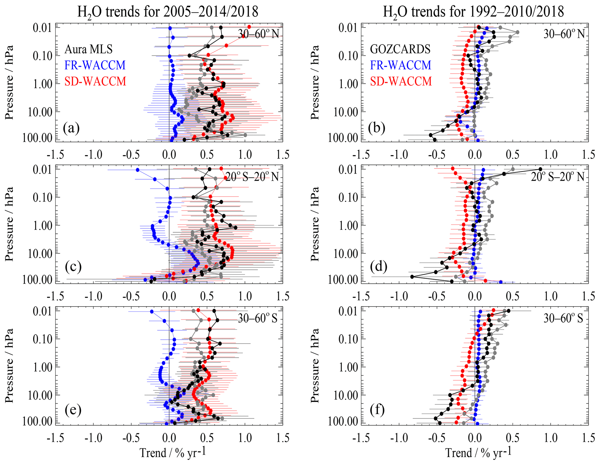
Figure 22Trends in three latitude bins for stratospheric and mesospheric H2O from an analysis of the 2005–2014/2018 MLS data and the two WACCM models for 2005–2014/2018 (a, c, e) and the 1992-2010/2018 time period (b, d, f); only the observational trend results are extended through 2018 (grey points) for MLS (a, c, e) and for GOZCARDS (b, d, f).
For H2O, there have been conflicting past results on stratospheric trends, depending on whether one investigates sonde or satellite data (e.g., Oltmans et al., 2000; Scherer et al., 2008), and regarding mechanisms that could account for more than a few tenths of a percent per year increase in H2O, as CH4 increases do not appear to be large enough for this. Changes in cold point temperatures or in the circulation need to be invoked in order to account for significant decadal-scale trends in H2O (e.g., Randel et al., 2000; Rohs et al., 2006; Tian and Chipperfield, 2006; Hegglin et al., 2014). Based on our analyses for 2005–2014, we find from Fig. 22 (a, c, and e) a positive H2O trend both in the MLS data and in SD-WACCM, which tracks observations (versus latitude as well as pressure) better than FR-WACCM does. FR-WACCM exhibits systematically smaller H2O trend values than both MLS and SD-WACCM at all pressures except near 100 hPa. The fact that FR-WACCM trend results for the 2005–2014 period are significantly smaller for the mid-stratosphere to lower mesosphere than the SD-WACCM and observed trends appears to mainly be a result of slightly different decadal variability in this run; we also see instances in longer time series (not shown) where FR-WACCM short-term changes appear to be larger than those from SD-WACCM. Finally, the FR-WACCM trends have smaller error bars, given the lower variability found in this model over the time period investigated here. With such lower variability, detection of a given trend would take less time than with the actual (observed) variability. The overlap for FR-WACCM and MLS is marginal in the upper stratosphere and lower mesosphere, where the impact on H2O from CH4 decomposition should be at its maximum, and cold point temperature variability issues are smaller than near the tropical tropopause; also, the solar cycle effects on the H2O time series are largest in the upper mesosphere (see also Froidevaux et al., 2015), but our regression analysis includes a solar flux term (see Appendix A3) and largely takes this effect out. For the longer timescale provided on the right side of Fig. 22, for H2O trends since 1992, we see that the upper-stratospheric and mesospheric trends are much closer to zero than for 2005–2014 or 2005–2018. We have used 2010 as the end year for the model comparisons here to minimize the impact of drifts in the MLS H2O trend results (see the next paragraph for further details); trend results for 1992–2018 are provided as a reference but should be considered as an upper limit, given this drift issue for (roughly) the last 8 years of MLS data. An analysis of H2O HALOE profiles and ground-based microwave profiles over Hawaii (Nedoluha et al., 2009) showed that changes in upper-stratospheric and mesospheric H2O were indeed sensitive to the solar cycle but showed only negligible overall trends between 1992 and 2008. We can also see this evidence for smaller trends in the earlier portion of the H2O record in time series (not shown here) from the GOZCARDS data set, with the stronger part of the trend coming after 2007 (as confirmed by the Fig. 22 results). The causes for CH4 changes over the past few decades have been difficult to identify with confidence (see Feldman et al., 2018; Turner et al., 2017). Simple algebra indicates that such CH4 changes can lead to only part (about half) of the H2O increases reflected in the 2005–2014 trends, and there must be other reasons for these fairly large short-term trends. We believe that the significant decadal variability in H2O, which arises from cold point temperature variability, propagated upward as a “tape recorder” signal, and QBO variability account for a large part of the large positive H2O trends for 2005–2014. Indeed, Garcia et al. (2007) noted in their studies of WACCM trends that multiple decades are likely needed to enable detection of the underlying secular rise in stratospheric H2O, given the variability arising from ENSO, cold point temperature changes, the QBO, and other factors. Also, a sudden drop in water vapor after 2000 can lead to a stronger post-2000 stratospheric H2O trend, if one is considering a rather short time period. In terms of the lower-stratospheric longer-term trend results, Fig. 22 (b, d, and f) shows that there have been some decreases since 1992 (and with the 1992–2018 results being viewed as an upper limit). Based on time series (not shown here), the models underestimate these decreases and show less variability, in terms of significant drops in water vapor as well as smaller positive oscillations; other factors that could contribute to these differences include the poorer atmospheric sampling prior to the MLS data and potential systematic uncertainties in the merged data set (which is a more difficult hypothesis to test).
We should also note that water vapor drifts have been detected between coincident MLS and sonde H2O data, mostly since about 2010, with MLS-derived trends being more positive than those from frost point profiles (Hurst et al., 2016). This relative drift (of as much as 0.5–1.6 % yr−1 for 2010–2015, depending on altitude and location) could play a role in some discrepancies between model (SD-WACCM) and MLS trends for 2005–2014, and it does complicate such comparisons. While SD-WACCM results agree well with MLS in Fig. 22 (a, c, and e), they would become larger than MLS (adjusted) results if one were to subtract more than about 0.3 % yr−1 from these MLS trends, although we should keep the error bars in mind. Possible causes for drifts between MLS and sonde H2O data are being investigated, with only a small part of this discrepancy currently attributable to a known instrument degradation issue for MLS H2O, which probably impacts other MLS data from the 190 GHz spectral region (notably N2O). We see that tropical H2O at 100 hPa (near the stratospheric water vapor entry level) does not display much of a trend. Previous studies of entry-level H2O using satellite data have concluded that no significant long-term trend is discernible (Hegglin et al., 2014; Dessler et al., 2014). The former study led to slightly negative lower-stratospheric H2O trends (although with no statistical significance). GOZCARDS H2O data used here, however, do not include SAGE II data back to the late 1980s, as was the case in the work by Hegglin et al. (2014), who also obtained positive long-term (1980–2010) trends in the upper stratosphere from satellite-derived H2O anomalies, merged using a global CCM as a transfer function. As found by others, especially when dealing with large decadal-type variability, the choice of start and end points, as well as the length of period studied, can significantly influence trend values, be it for H2O or O3. Lower-stratospheric H2O trend detection is rendered difficult by such variability, including significant short-term changes (Randel et al., 2006; Hurst et al., 2011; Fueglistaler, 2012; Urban et al., 2014), as noted here also (see Fig. S12).
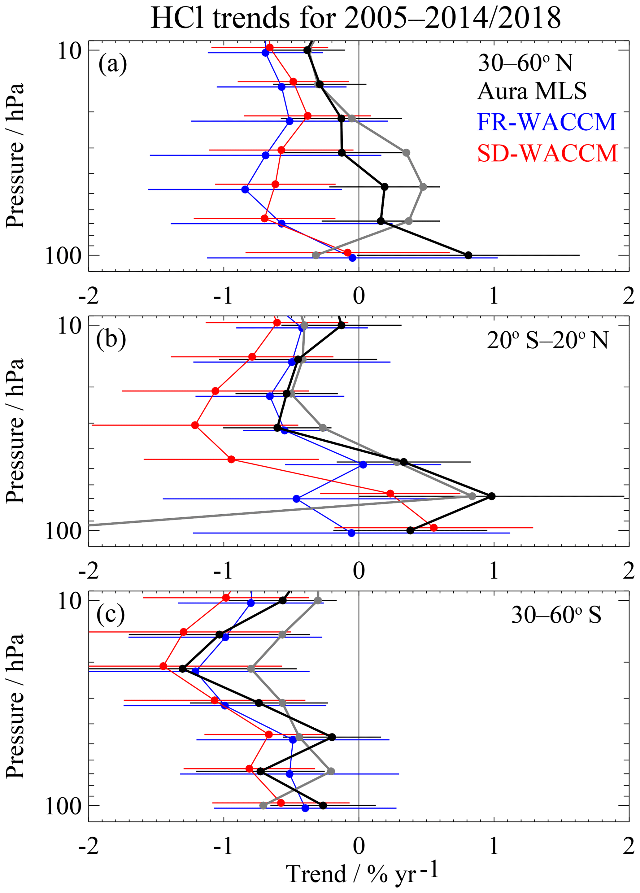
Figure 23Same as Fig. 19 but for lower-stratospheric MLS HCl data trends for 2005–2014/2018 (with grey points showing MLS results through 2018) and WACCM HCl trends for 2005–2014.
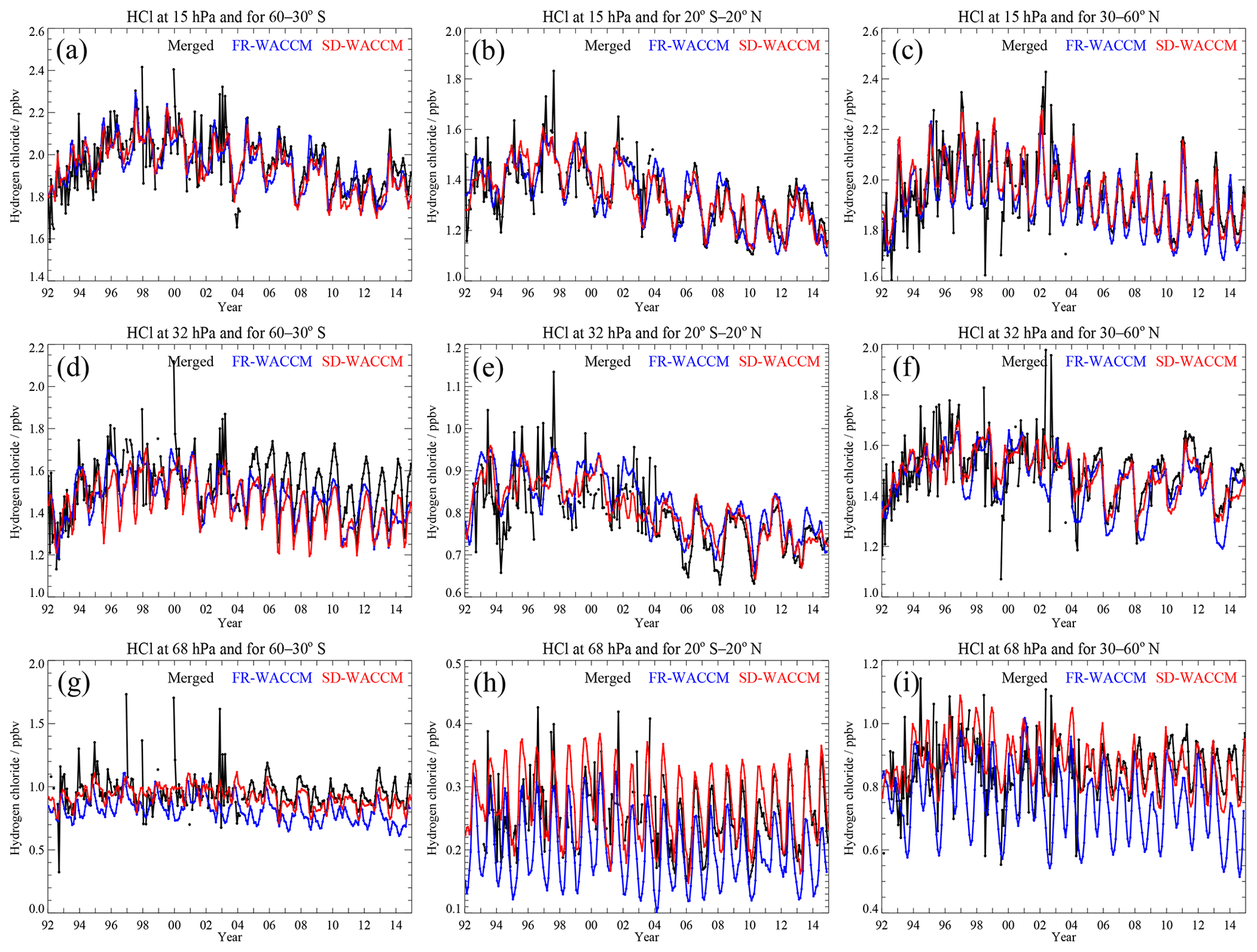
Figure 24Time series (1992–2014) of lower-stratospheric HCl (ppbv) for the GOZCARDS HCl merged data record (black), as well as models (FR-WACCM in blue and SD-WACCM in red). Each panel is for a different pressure level and latitude bin, as labeled (15 hPa, a–c; 32 hPa, d–f; 68 hPa, g–i); the three latitude bins used in this work are 30–60∘ S (a, d, g), 20∘ S–20∘ N (b, e, h), and 30–60∘ N (c, f, i).
For HCl, changes in stratospheric values have been nonlinear, with a rapid rise prior to 1998 and a slower decrease after 2004, as expected from time-shifted abundances of total surface chlorine (Froidevaux et al., 2015). Focusing first on 2005–2014/2018, we show model and data HCl trends for the lower stratosphere in Fig. 23. The agreement between SD-WACCM and MLS trends (for 2005–2014) is good, especially for 30–60∘ S, although the error bars are fairly large. However, the (negative) HCl trend results from both models lie below the observed trends almost everywhere. The upper portion of this model–data bias follows what we observe also in the upper stratosphere (not shown), where MLS-derived HCl trends are too shallow compared to expectations (from model and surface-derived chlorine trends), whereas upper-stratospheric trends from the original MLS HCl product were more negative (see Froidevaux et al., 2006; Livesey at al., 2018). As a reminder, the MLS team recommends that data users not include upper-stratospheric MLS HCl data (post-2006) in any trend studies. For the lower stratosphere, where the HCl line is broader, there is less concern about the inability to track the HCl trend. Also, the near-zero drifts (drifts <0.1 % yr−1) obtained between two separate MLS O3 band retrievals (not shown), one from the same radiometer as HCl and one from the main (very stable) standard MLS O3 product (see Hubert et al., 2016), provide some confidence regarding the stability of LS HCl trends. At low latitudes, MLS HCl shows a positive tendency (largest at 68 hPa, per Fig. 23), albeit with marginal significance. The vertical gradient in these trends is duplicated fairly well by the SD-WACCM results, although the model trends are usually less than those from MLS. Latitude–pressure trend variability, including positive tendencies, could be related to circulation changes, as implied by analyses of short-term increases in lower-stratospheric HCl seen in both ground-based and GOZCARDS data (Mahieu et al., 2014). For the most part, the MLS trend results for HCl do not change appreciably when we consider the longer period through 2018 (grey points in Fig. 23). Given the rapid rise in chlorine prior to 1998 and the nonlinear changes near the peak period, we show in Fig. 24 lower-stratospheric time series from GOZCARDS merged HCl (Froidevaux et al., 2015) and WACCM for 1992–2014. There is fairly good agreement in the nonlinear behavior observed in both data and model series. The scatter in HCl data decreases after 2005, and the earlier time series suffer from more inhomogeneous sampling, which may at least in part explain the larger scatter and model–data differences (there is no attempt here to sample models within each month like the data, and this would be difficult for a merged data set). There are also regions and periods of slow HCl increases in both data and models (Fig. 24), as well as hemispheric differences in short-term tendencies (Mahieu et al., 2014; Froidevaux et al., 2015). The HCl time series are tracked well by SD-WACCM, which generally matches the data better than FR-WACCM; this is consistent with the understanding that dynamically driven variations are better captured by the incorporation in SD-WACCM of realistic meteorological fields (MERRA). Stolarski et al. (2018) investigated the removal of dynamical variability from MLS lower-stratospheric HCl series by using MLS N2O data as a fitting function in the regression; this led to HCl trends that match expectations based on changes in surface chlorine. The search for detailed explanations of such short-term increases and variability in lower-stratospheric HCl (and other composition changes) continues to be an interesting area of investigation.
In the upper stratosphere, it has been difficult to explain the details of observed HCl variations from 1998 to 2002, including the dip between these years (Waugh et al., 2001). We show in Fig. S16 near-global (60∘ S–60∘ N) GOZCARDS HCl series at 1 hPa. This shows a systematic model underestimate of HCl in the uppermost stratosphere; the model–data difference is much smaller at pressures closer to 5 hPa. While the systematic uncertainties (of ∼0.2 ppbv) in the data encompass the model values, the model total should be increased by the chlorine contribution from very short lived halogenated substances (VSLS) to the stratosphere; although this contribution is only of order 0.1 ppbv (Carpenter et al., 2014), recent evidence suggests that there could be a somewhat larger stratospheric chlorine contribution from VSLS (Oram et al., 2017). Nevertheless, the historical maximum for total tropospheric chlorine was about 3.65 ppbv (WMO, 2014), and this should be the maximum total chlorine expected in the uppermost stratosphere. While WACCM includes the proper abundance and evolution of chlorine source gases, maximum WACCM HCl in the upper stratosphere (and lower mesosphere) is just under 3.4 ppbv. It is also interesting that the gap between the models (both versions) and the data worsens from 1992 to 2000, with the HCl peak occurring later in the data (with a broader peak than in the models). After about 2002, the decrease in near-global HCl roughly follows the model decrease; additional years of HCl data from ACE-FTS should help refine this comparison. In terms of HCl trends, Hossaini et al. (2019) have recently shown that there are positive changes (by ∼15 %) in model upper-stratospheric HCl trends since 2000, i.e., the HCl decreases are smaller, if one takes into account the likely impact of changes in stratospheric chlorine from VSLS.
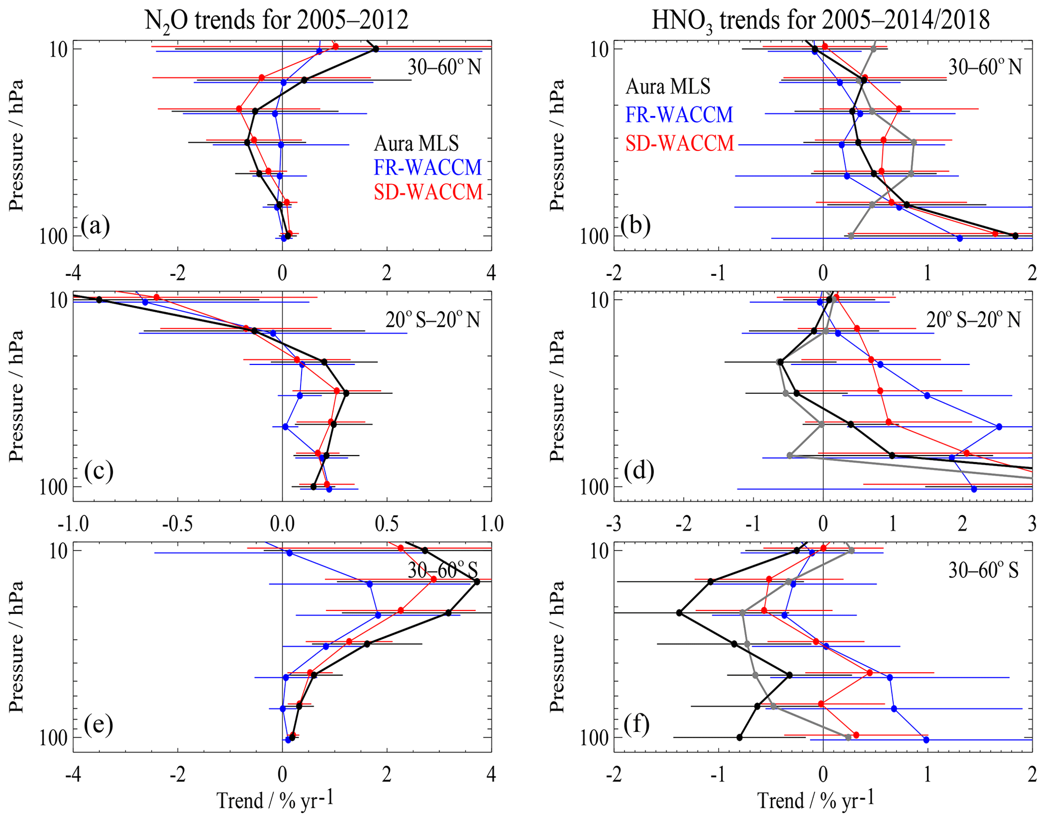
Figure 25Same as Fig. 23 but for N2O (a, c, e) and HNO3 (b, d, f) data and model trends in the lower stratosphere. The N2O data results are from the N2O–640 MLS product (retrieved from the 640 GHz radiometer band data), which was discontinued in 2013 because of an instrument issue affecting this band (see text), and these data and model trends apply to the 2005–2012 period. The HNO3 trend results (data and models) are for 2005–2014, with additional data results (in grey) for 2005–2018.
For N2O and HNO3, lower-stratospheric model trends are compared to the corresponding MLS data trends in Fig. 25. We note that the MLS standard product right after launch was N2O–640 (retrieved from the 640 GHz radiometer data), but it was discontinued after mid-2013, as a result of a hardware degradation issue affecting that band (N2O only). The current MLS product, N2O–190, is retrieved from the 190 GHz band. Figure S17 provides evidence of negative drifts in lower-stratospheric N2O–190, apparently accelerating in the last few years, since the SD-WACCM and actual N2O values would be expected to continue to rise slowly after the end date on this plot, notably in the tropical lower stratosphere, where N2O should follow tropospheric trends. Indeed, tropospheric N2O has been increasing at a fairly steady rate of ∼0.26 % yr−1 (WMO, 2014), consistent with the model N2O and MLS N2O–640 lower-stratospheric increases at low latitudes (see Fig. S17 and especially the tropical trends in Fig. 25 at 100 hPa). FR-WACCM N2O trends show slightly poorer agreement than SD-WACCM versus N2O–640, although this is not statistically significant. Tropical lower-stratospheric MLS N2O–190 trends (not shown) are negative (albeit with error bars that encompass small positive trends) but show some differences versus expectations and the N2O–640 results. As for HCl, interhemispheric differences in lower-stratospheric N2O trends are interesting in terms of their implications for effects relating to transport (age of air) and changes in the circulation. At lower pressure values, the N2O trends do not mirror the tropospheric N2O trends (in % yr−1), and other factors play a role (changes in circulation, QBO, N2O photodissociation). The asymmetry in age of air obtained by analyses of (2002–2012) MIPAS SF6 data (Haenel et al., 2015) could also be related to asymmetries in N2O tendencies. They found relatively older air in the northern extra-tropics and younger air in the southern extra-tropics; this could also imply opposite trends for N2O between southern and northern lower stratosphere. However, Bönisch et al. (2011) have pointed out that tracers (e.g., O3 and N2O) can be impacted differently by both vertical and quasi-horizontal transport effects, depending on their relative vertical and meridional gradients. Moreover, their work indicates that detailed attribution of tracer variations to structural changes in the Brewer–Dobson circulation is a complex matter, and short-term and longer-term changes may well have different characteristics. Our work mainly identifies similarities between some of the trend patterns versus pressure and latitude from SD-WACCM, in particular, and the observed trends, for a fairly short-term period. For the HNO3 trends (Fig. 25), we see fairly good agreement between models and data for 2005–2014; latitudinal tendencies and interhemispheric differences therein are similar for model and data. The spatial gradients of these species are different in the lower-stratosphere (HCl and HNO3 increase with height, in contrast to N2O), and we see that the decreasing HCl trends for 2005–2014 at 30–60∘ S (Fig. 23), in particular, are qualitatively similar to those from HNO3 in this region. For lower-stratospheric HNO3, there is an underlying trend part caused by the slow increases in N2O, as we can observe in longer-term (1980 to present) model time series (not shown here), but more abundant volcanic aerosols also led to large HNO3 changes, tied to heterogeneous chemistry, in the 1980–1992 time period. N2O and H2O (source gases for HNO3) are significantly affected by the QBO, and there is a strong related variability in lower-stratospheric HNO3. Observed short-term trend patterns in HCl, HNO3, and N2O are better captured by SD-WACCM, overall, than by FR-WACCM, as we show in Fig. S18 for the 2005–2010 period, which is relevant to the results of Mahieu et al. (2014), who emphasized short-term HCl increases during this time. We note the correlation in these short-term trend results for HNO3 and HCl but an anti-correlation for N2O versus HCl (and HNO3). Figure 25 also shows that the inter-hemispheric asymmetry in trends for lower-stratospheric HNO3 has persisted for the 2005–2018 period, although longer-term SD-WACCM results (not shown) indicate that this is not modeled as a stable pattern over several decades. Such short-term tendencies and correlations (or anti-correlations) were also noted by Douglass et al. (2017), who emphasized the results from various column time series, from both observational records and model simulations (including modeled age of air).
We have analyzed stratospheric data (and mesospheric data as well for H2O) in terms of absolute abundances, variability, and trends for several species (O3, H2O, HCl, N2O, and HNO3), based on 10–14 years of Aura MLS measurements, as well as longer-term data records from GOZCARDS (for O3, H2O, and HCl). While our emphasis here has been on model evaluation and comparisons for two types of chemistry–climate model runs (the free-running and specified dynamics versions of CESM1 WACCM), we also point out certain observational highlights regarding stratospheric change, notably using recent MLS data through 2018. Our conclusions are thus largely separated in terms of (1) updates regarding atmospheric variations and trends, mostly for the 60∘ S–60∘ N region; and (2) model evaluation aspects, for comparisons through 2014 only.
Regarding the more novel highlights from satellite data analyses, we have used multiple linear regression to derive trends based on zonal mean time series from Aura MLS data alone, between 60∘ S and 60∘ N. In the upper stratosphere, MLS O3 data show increases over 2005–2018 at a rate of ∼0.1–0.3 % yr−1 (depending on altitude and latitude) with 2σ uncertainties of ∼0.2 % yr−1 (or less, for near-global averages). For the lower stratosphere (LS), GOZCARDS O3 data for 1998–2014 point to small decreases for broad latitude regions between 60∘ S and 60∘ N (as obtained also by Ball et al., 2018), but we obtain more positive trends if the starting year is 2005. The SH midlatitudes (30–60∘ S) exhibit LS trends for 1998–2018 that are near zero (or slightly positive). The LS O3 trends based on 2005–2018 MLS data are most positive at these SH midlatitudes (with trends of 0.1–0.2 % yr−1, although marginally statistically significant), in contrast to slightly negative or near-zero trends for 2005–2014. Also, at northern midlatitudes in the lower part of the stratosphere, a significant drop in O3 trends is obtained between the 2005–2014 results (0.5–0.9 % yr−1) and 2005–2018 (near-zero trends). Given the high variability in LS O3, and the high sensitivity of trends to the choice of years used, especially for short time periods, further studies of this region are required for a more robust longer-term trend result. Only careful analyses of additional years of high-quality data can help to elucidate this question. For H2O, upper-stratospheric and mesospheric trends based on GOZCARDS 1992–2010 data are near zero (within ∼0.2 % yr−1) and significantly smaller than trends (within ∼0.4–0.7 % yr−1) from MLS for 2005–2014 or 2005–2018. As shown before by others, there are multiple factors that can influence low-frequency variability in H2O; these recent stratospheric short-term positive trends go beyond what one would expect from changes associated with a slow, secular increase in methane, even if some of the recent CH4 changes have been nonlinear (Schaefer et al., 2016; Nisbet et al., 2016). However, given the known drift in MLS H2O series (mainly since 2010) versus in situ sonde data (Hurst et al., 2016), the MLS trends above should be viewed as upper limits. We also note that the very shallow solar flux maximum (in 2011 to 2014) of solar cycle 24, with lower-than-usual flux, led to a more extended period of large mesospheric H2O since the minimum values observed in GOZCARDS time series in 2002 (see Froidevaux et al., 2015); this has contributed to the fairly large short-term mesospheric and upper-stratospheric H2O trends since 2005. For HCl, the MLS data show regions and periods of small HCl increases in the lower stratosphere, within the context of the longer-term stratospheric decrease in HCl, as well as interhemispheric–latitudinal differences in short-term HCl tendencies. We observe similarities in such short-term tendencies, and interhemispheric asymmetries therein, for lower-stratospheric HCl and HNO3, while N2O trend profiles exhibit anti-correlated patterns. Some studies have implied that such short-term trends relate to changes in age of air and circulation, and this is the subject of continuing analyses. More generally, we are reminded through such work that, especially when dealing with large decadal-type variability, the choice of start and end points, as well as the length of period studied, can significantly influence the resulting trend values, and certainly the shorter-term tendencies.
In terms of the model evaluation analyses, climatological averages for 2005–2014 from FR-WACCM and SD-WACCM for O3, H2O, HCl, N2O, and HNO3 compare generally favorably (within 2σ systematic errors) with Aura MLS data averages over this period. Model O3 values are usually within ±5 %–10 % of the data, except in the UTLS. In the lowest stratosphere, SD-WACCM generally exceeds the observed ozone means by 30 %–50 %, with FR-WACCM showing a smaller overestimate; both models also overestimate (by ∼60 %) the amplitude of the annual cycle in this region. Such differences require further investigations but would appear to implicate, in part, a transport-related issue in the models. For H2O, there is a model low bias (by 5 %–15 %) versus MLS data in the upper stratosphere and most of the mesosphere, although some of this might be a result of a small high bias in MLS H2O versus other satellite data (Hegglin et al., 2013). Also, the models significantly underestimate average HNO3 values in the upper stratosphere, notably at high latitudes; this stems from the known effects of missing model ion chemistry, as it relates to particle precipitation effects in the mesosphere, followed by downward wintertime polar transport of enhanced NOx, and subsequent increases in HNO3. In the lower stratosphere at high southern latitudes, variations in polar winter and spring composition observed by MLS are generally well matched by SD-WACCM, with the main exception being for the early winter rate of decrease in HCl, which is too slow in the model (see also the work on this topic by Grooß et al., 2018). Regarding the fitted variability tied to the AO and SAO, there are a few discrepancies between model-derived amplitude patterns and the corresponding MLS climatology features, but FR-WACCM and SD-WACCM appear to properly capture the primary processes governing these modes of variability. We have provided diagnostics for the fits between WACCM runs and MLS deseasonalized anomaly series. These include correlation coefficients for different time series as well as a diagnostic of rms differences (model versus data) divided by the rms data variability. Not too surprisingly, SD-WACCM, which is driven by realistic dynamics, generally matches the observed zonal monthly mean anomalies significantly better than does FR-WACCM; this holds for all five species that we considered, with larger values of R2 and smaller values of the rms difference diagnostic for SD-WACCM.
For a more fair and useful metric of model quality, in particular for a free-running model, we have compared the rms interannual variability from the anomalies in both WACCM models versus observations. One of the main features is that the H2O variability from the lower stratosphere to upper mesosphere is underestimated by both models; this underestimate can reach a factor of 2, although more typically it is of order 30 %. This implies that more years (by a factor of 1.2 to 1.6) would be needed to detect an actual trend in H2O than if one used the WACCM-based predictions. Ozone variability is better represented by WACCM, with model/data variability ratios typically within a factor of 0.8 to 1.2. Observed HCl variability is underestimated somewhat by FR-WACCM for 1992–2003 but not for 2005–2014; the sparser HALOE sampling, compared to MLS, could explain some of the underestimate for the early period, especially in polar regions. For N2O, there is also a model underestimate (from both WACCM versions) of MLS-derived LS low-latitude variability, although this variability is small.
Regarding trends, the model comparisons versus the O3 data records from GOZCARDS (version 2.20) show generally good qualitative agreement in the time series for both upper- and lower-stratospheric change; the WACCM O3 trends estimated using the same regression model as used for the MLS data show good agreement with the data trends. Furthermore, the observed trend dependence on latitude and pressure is matched quite well by the SD-WACCM trend results. We have not considered the high latitudes in detail here, in part because of the significant dynamical variability in that region. Stone et al. (2018) recently analyzed model results at high latitudes in the upper stratosphere and showed that the large variability in that region, including the effects of solar proton events, is likely to mask detection of recovery (for now). In the lower stratosphere, where larger variability exists, the O3 trends we deduce from the data and models agree within fairly large error bars (and generally with no statistical significance). For 2005–2014, the SD-WACCM trends seem to track the observed positive O3 tendencies, although with marginal statistical significance. For H2O, the MLS and SD-WACCM positive trend results agree fairly well, but FR-WACCM shows significantly smaller increases; this discrepancy for FR-WACCM is even more pronounced for the longer-term GOZCARDS H2O records (since 1992). Larger discrepancies for FR-WACCM likely arise from its poorer correlations (than SD-WACCM) with cold point temperatures and with QBO variability. For HCl, our trend analyses reveal broad agreement between the lower-stratospheric MLS data (2005–2014) and the models, but with some systematic differences. While decreases in global LS HCl are indicated for 2005–2014, there are some observed hemispheric differences, and some increase is suggested in tropical MLS data at 68 hPa, where there is only a slight positive trend from SD-WACCM. While the vertical gradients of MLS HCl trends are duplicated to some extent by SD-WACCM, the model trends are always more negative. We see a continued need for more comparisons of the various HCl measurements, satellite-based and ground-based, as well as for model comparisons, in order to better understand circulation influences on stratospheric composition, as well as potential measurement-related issues. Part of the model–data systematic difference in HCl trends could be explained by the omission (in WACCM) of the impact of VSLS on stratospheric chlorine, as indicated by the recent work of Hossaini et al. (2019). For N2O, the interhemispheric asymmetry in MLS-derived trends (for 2005–2012), with negative trends (of up to −1 % yr−1) at NH midlatitudes and positive trends (of up to 3 % yr−1) at SH midlatitudes, is in agreement with the asymmetry in SD-WACCM results. Small observed positive trends of ∼0.2 % yr−1 in the 100 to 30 hPa tropical region are consistent with model results, which in turn are very close to the known rate of increase in tropospheric N2O (at about +0.26 % yr−1; see WMO, 2014). In the case of HNO3, the MLS-derived lower-stratospheric trend differences (for 2005–2014) between hemispheres are opposite in sign to those from N2O (whose spatial gradients are largely of a sign opposite to those from HNO3) and in reasonable agreement with both WACCM results, despite large error bars. While more detailed analyses would be needed to try to relate such trend asymmetries to changes in age of air, or circulation, we note that the QBO is a large contributor to such short-term trend results in the middle stratosphere.
The diagnostics provided in this WACCM model evaluation can help distinguish even fairly subtle differences between models and observations, as well as between models. Further collaborations between modeling groups and instrument teams, as well as continuing data validation, will help to expose and clarify species-dependent instrumental effects (biases or drifts). Finally, independent CCMs are not created in the same way, and nudging approaches can vary; in addition, some models have an internally generated QBO, but most do not. While this study focused on CESM1 WACCM, continuing studies of the differences between high-quality observations and various models of atmospheric composition will be useful. Such work could be expanded to include species not considered here and/or with more of a focus on the upper troposphere.
Aura MLS data used in this work are monthly zonal means derived from Level 2 MLS data, which are accessible from the Goddard Earth Sciences Data and Information Services Center (GES DISC), funded by NASA's Science Mission Directorate; a link for MLS Level 2 data access can be found at https://mls.jpl.nasa.gov/data/ (last access: 4 April 2019). GOZCARDS data sets can be obtained (by entering GOZCARDS in the search) at http://disc.gsfc.nasa.gov (e.g. Anderson et al., 2013; Froidevaux et al., 2013; Wang et al., 2013). More recent years (and version updates) will be made available at this site or can be obtained by request to the first author. The WACCM model output used here is provided in some of the references and is available from the NCAR Earth System Grid at https://www.earthsystemgrid.org/search.html?Project=CCMI1 (last access: 4 April 2019). For WACCM, we thank NASA Goddard Space Flight Center for the MERRA data (accessed freely online at http://disc.sci.gsfc.nasa.gov/, last access: 4 April 2019).
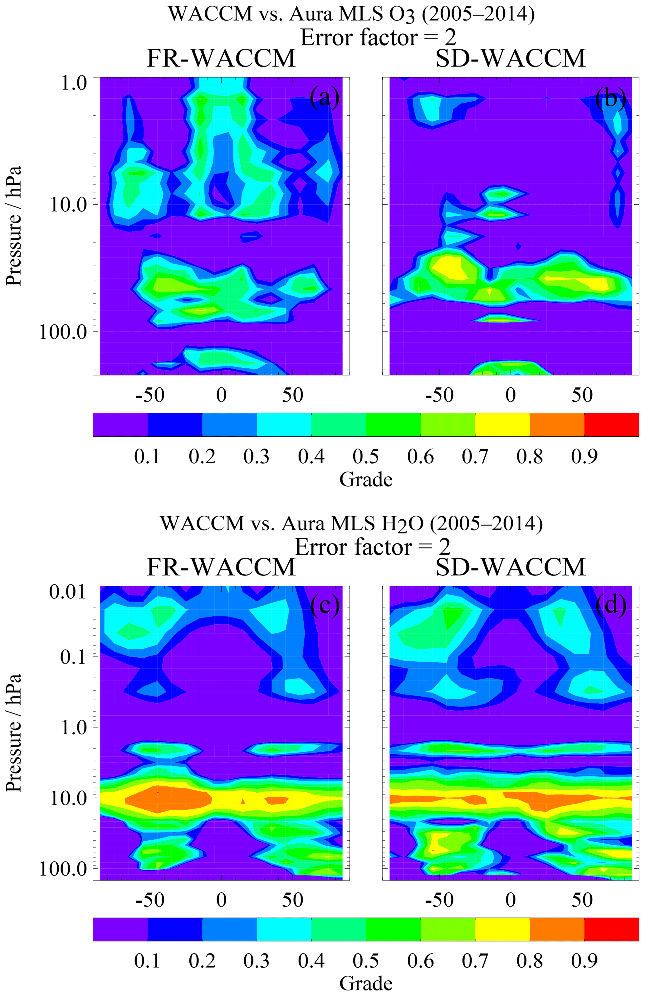
Figure A1Examples of grades for model evaluations of O3 (a, b) and H2O (c, d), using a grading methodology that has been used in the past (see Eq. A1), applied to both FR-WACCM (a, c) and SD-WACCM (b, d) time series versus Aura MLS time series from 2005 through 2014. These grades are for an error factor of 2 (in Eq. A1).
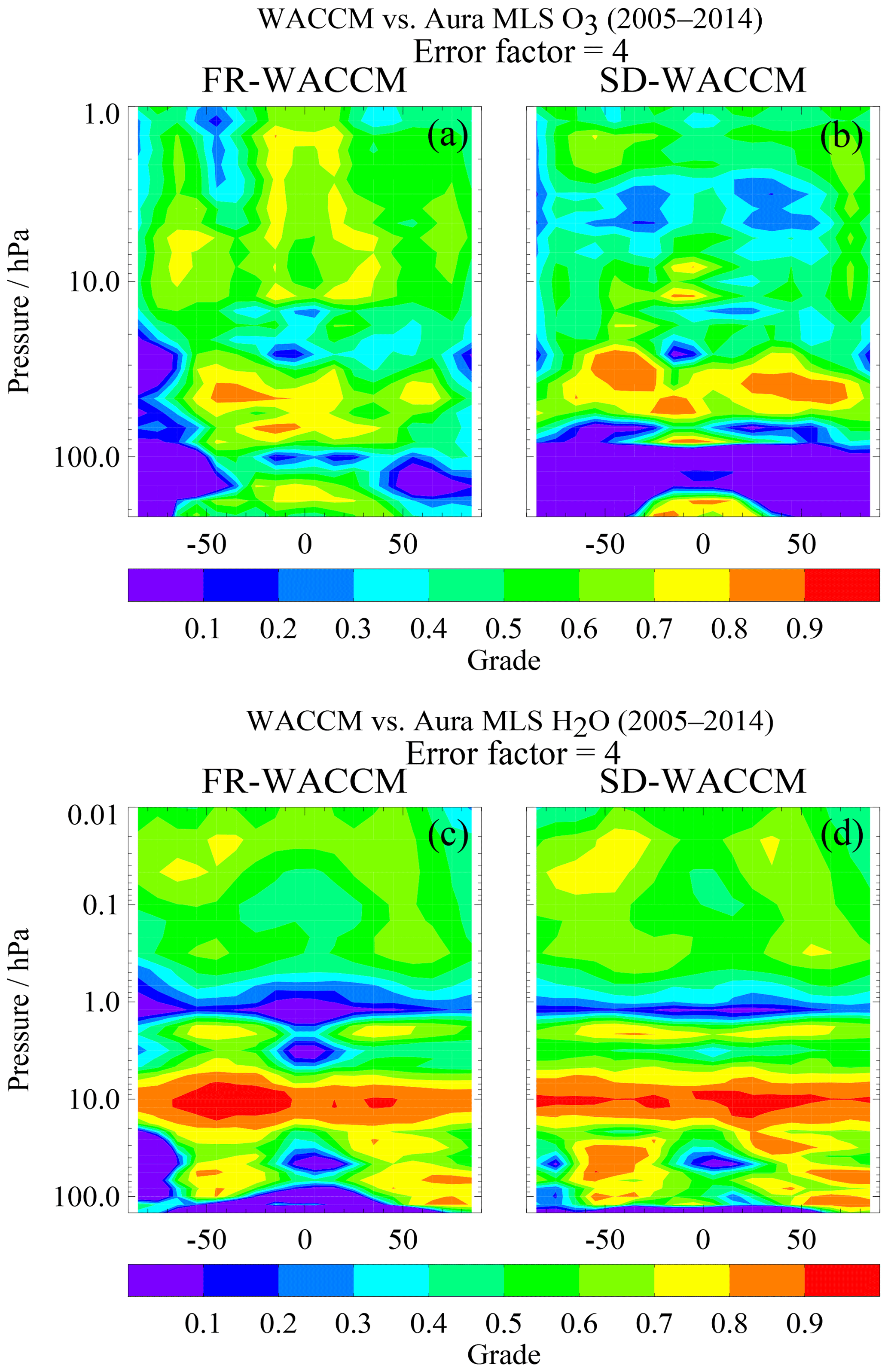
Figure A2As in Fig. A1, for model evaluation grades of O3 and H2O (WACCM versus Aura MLS data), but for a value of 4 (rather than 2) for the error factor (see Eq. A1).
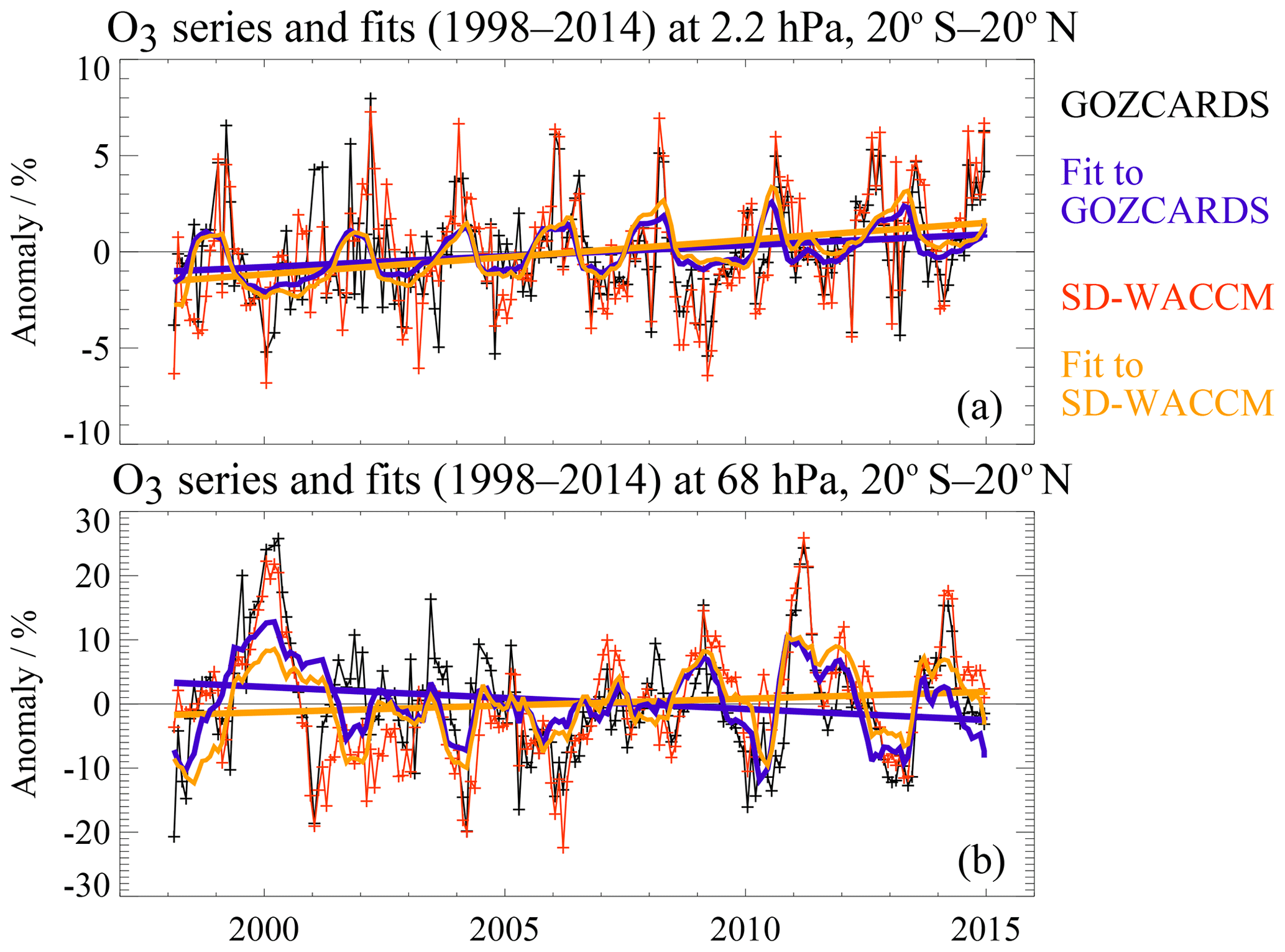
Figure A3Deseasonalized monthly mean anomaly time series for O3 (%) at 2.2 hPa (a) and 68 hPa (b), for 1998 through 2014, for averages over 20∘ S–20∘ N. Note that the y axis range for 68 hPa (b) is 3 times larger than for 2.2 hPa (a). The data set (black) is from the GOZCARDS ozone record, with the SD-WACCM (simulated) series (red) also shown. Fits to the observational series are in purple, and fits to the model series are in orange; the fitted time series functions (curves) and the fitted linear components (straight lines) are shown.
A1 Examples of other model evaluation methods
A grading method that has been applied in some previous comparisons (for example see Douglass et al., 1999; Waugh and Eyring, 2008) between atmospheric model values (Mn) and observed values (On) utilizes Eq. (A1) below to arrive at grades between 0 and 1 (and if a grade is <0, it can be set to 0):
with index n (in a given time series) varying between 1 and N (the total number of monthly values being compared for a given latitude–pressure bin) and σn representing the error in the observations. While the error factor Ef should probably be set to 2 or 3, this gives grades that are too small (close to zero or negative) if one applies such a formula to the MLS O3 or H2O time series, specifically to data sets with pretty well defined total measurement errors (provided as 2σ error estimates, per Sect. 4, meaning an error factor of 2). The grades shown here in Figs. A1 and A2 correspond to error factors (Ef) of 2 and 4, respectively. Figure A2 leads to O3 and H2O grades that are more useful than Fig. A1. It also shows some similarities with the diagnostics based on percent differences between model and data shown in Sect. 4.
We note, however, that it is generally more difficult to estimate systematic errors for merged data records. The GOZCARDS data analyses led to somewhat pessimistic (or conservative) systematic error estimates (see Froidevaux et al., 2015), and these are significantly larger than error estimates for MLS data only. Other methods could lead to useful error estimates, through the use of multi-satellite data sets and the spread between these (see SPARC, 2017), for some species at least. Moreover, when one considers anomaly time series, it becomes even less clear how to best assign uncertainties in the context of error-weighted grades. Some data records may also drift with respect to others, or with respect to ground-based data, so that the actual errors will change with time (and possibly location). In the end, the most important aspect of model evaluation or grading analyses may lie in the relative values of grades or diagnostics for different models.
A2 The rms difference diagnostic
Given a model time series Mi(t) and an observational time series (both series here representing deseasonalized anomalies) Oi(t), the difference values between the two anomaly series are simply given by
and the root mean square (rms) of these anomaly differences (rmsdif) is expressed as
The rms value (variability) of the observational series (of anomalies) in this case is
One of the diagnostics that we use in Sect. 4 to compare how well different models match up with the observed time series is given by the ratio of the above variability values:
A3 Regression model
A3.1 Functional form
The MLR model and fitting methodology used here are similar to the methods used by many others in the past, with a linear model description that uses annual, semiannual, QBO, and ENSO terms. Thus, the model function to be fitted for coefficients a, b, cn, dn, f1, f2, f3, and f4 has the familiar form:
with the (monthly series) time variable expressed by t and tm chosen as the series midpoint; the linear trend term is coefficient b above. The sine and cosine functions provide for periodic variations with periods Pn. For our work, we use the primary shorter-term periodic oscillations, namely the annual (12-month period) and semiannual (6-month period), in Eq. (A6), in addition to shorter-term periodic terms (with 3- and 4-month periods); such short-term variability helps to produce better fits and can reduce error bars slightly, although the resulting linear trend results are not affected much. The QBO is also a major source of variability in stratospheric composition time series. As a QBO proxy, we include the variability in monthly mean tropical wind series; we use the linear combination of (roughly orthogonal) equatorial wind series at 50 and 30 hPa as the QBO1 and QBO2 functions above to account for phase shifts in the series at different locations. Monthly mean zonal equatorial wind data are made available by the Freie Universität Berlin (see http://www.geo.fu-berlin.de/en/met/ag/strat/produkte/qbo/, last access: 10 January 2019, for data access information and references). We have also tested fits with the zonal mean wind vertical shear (gradient) rather than the wind itself as a proxy, but this did not make significant changes in the trends (or improvements in the residuals). The ENSO proxy follows the monthly mean Multivariate ENSO Index (MEI), which combines data from six main geophysical variables over the tropical Pacific (see Wolter and Timlin, 1993, 1998; https://www.esrl.noaa.gov/psd/enso/mei/index.html, last access: 10 January 2019). Also, we have included an 11-year solar cycle proxy term (see the last term in the above equation), using the monthly averaged 10.7 cm solar flux time series kindly provided (see ftp://ftp.geolab.nrcan.gc.ca/data/solar_flux/monthly_averages, last access: 10 January 2019) by the Canadian Space Weather Forecast Centre. For further discussions of alternate fitting methods (e.g., methods using effective equivalent chlorine time series as a proxy), the reader is referred to the abundant literature on trend assessments (see WMO, 2014, and references therein). Our main goal here is to retrieve trends and trend errors from the data and the models in the same way. An example of deseasonalized tropical ozone time series at two pressure levels is given in Fig. A3, which shows MLS and SD-WACCM series, along with the fits and the linear trends.
A3.2 Trend errors
For the evaluation of error bars in the linear trends, we have used the method of bootstrap resampling (Efron and Tibshirani, 1986). As others have done for ozone trend analyses (Randel and Thompson, 2011; Bourassa et al., 2014), we have applied this using block bootstrapping (using yearly blocks of data), thereby preserving some of the dependency in the time series. Basically, one samples and (randomly) replaces blocks of yearly data for a large number of resampling cases (on linear fits to the residuals) and then calculates the standard deviation of this large number of trend results to arrive at trend uncertainties; note that we use 2σ values as error bars in our comparisons (which is very close to 95 % bounds). We have used 20 000 samples in our bootstrap analyses; changing this number (e.g., by several thousand) does not alter the results significantly, as long as one chooses a large enough total number of cases. An alternative method is to attempt to correct trend uncertainties for the autocorrelation of the residuals after the regression fit (Tiao et al., 1990; Weatherhead et al., 1998; Santer et al., 2000). The existence of nonrandom residuals effectively implies that the number of independent data points is less than the number making up the original time series. The end result is that trend uncertainties are larger than if one neglects these effects. We find that trend errors from this bootstrap method for our time series examples are often larger than more simplistic/standard calculations by factors ranging from about 1.2 to 2 or more. We have checked our trend error calculations with the OSIRIS team (Christopher Roth, personal communication, 2018) based on a sample time series, as we have used the same block bootstrap approach as they have (see also Bourassa et al., 2014).
The supplement related to this article is available online at: https://doi.org/10.5194/acp-19-4783-2019-supplement.
LF produced the majority of this paper, including the figures. DK provided the model runs used in these comparisons to observational data from Aura MLS and GOZCARDS; he also described the models used here and provided substantial guidance and comments for this paper. HJW and JA, along with LF, were key participants in the development and creation of the GOZCARDS data sets, including the recently updated version (2.20) for merged ozone used herein. RF was another key participant in the GOZCARDS data production, and he also provided programming support for these model intercomparisons.
The authors declare that they have no conflict of interest.
This article is part of the special issue “Chemistry–Climate Modelling Initiative (CCMI) (ACP/AMT/ESSD/GMD inter-journal SI)”. It is not associated with a conference.
Work at the Jet Propulsion Laboratory, California Institute of Technology, was performed under contract with the National Aeronautics and Space Administration (NASA). GOZCARDS data were initially produced under the NASA Making Earth System Data Records for Use in Research Environments (MEaSUREs) program, with data continuity/updates now provided under MLS funding. We acknowledge insights and comments regarding aspects of this work from Rolando Garcia, Nathaniel Livesey, Jessica Neu, and Michelle Santee. We also appreciate discussions and comparison work regarding trends and error bars with Doug Degenstein and Chris Roth, as well as Emmanuel Mahieu (and via some of his European contacts). The National Center for Atmospheric Research (NCAR) is sponsored by the U.S. National Science Foundation (NSF). WACCM is a component of NCAR's Community Earth System Model (CESM), which is supported by the NSF and the Office of Science of the U.S. Department of Energy. Computing resources for WACCM were provided by NCAR's Climate Simulation Laboratory, sponsored by NSF and other agencies; we also acknowledge the computational and storage resources of NCAR's Computational and Information Systems Laboratory (CISL).
This paper was edited by Gunnar Myhre and reviewed by three anonymous referees.
Anderson, J., Froidevaux, L., Fuller, R. A., Bernath, P. F., Livesey, N. J., Pumphrey, H. C., Read, W. G., Russell III, J. M., and Walker, K. A.: GOZCARDS Merged Water Vapor 1 month L3 10 degree Zonal Means on a Vertical Pressure Grid V1.01, Greenbelt, MD, USA, Goddard Earth Sciences Data and Information Services Center (GES DISC), https://doi.org/10.5067/MEASURES/GOZCARDS/DATA3004, 2013.
Andersson, M. E., Verronen, P. T., Marsh, D. R., Pälvärinta, S.-M., and Plane, J. M. C.: WACCM-D-Improved modeling of nitric acid and active chlorine during energetic particle precipitation, J. Geophys. Res.-Atmos., 121, 10328–10341, https://doi.org/10.1002/2015JD024173, 2016.
Ball, W. T., Alsing, J., Mortlock, D. J., Rozanov, E. V., Tummon, F., and Haigh, J. D.: Reconciling differences in stratospheric ozone composites, Atmos. Chem. Phys., 17, 12269–12302, https://doi.org/10.5194/acp-17-12269-2017, 2017.
Ball, W. T., Alsing, J., Mortlock, D. J., Staehelin, J., Haigh, J. D., Peter, T., Tummon, F., Stübi, R., Stenke, A., Anderson, J., Bourassa, A., Davis, S. M., Degenstein, D., Frith, S., Froidevaux, L., Roth, C., Sofieva, V., Wang, R., Wild, J., Yu, P., Ziemke, J. R., and Rozanov, E. V.: Evidence for a continuous decline in lower stratospheric ozone offsetting ozone layer recovery, Atmos. Chem. Phys., 18, 1379–1394, https://doi.org/10.5194/acp-18-1379-2018, 2018.
Bandoro, J., Solomon, S., Santer, B. D., Kinnison, D. E., and Mills, M. J.: Detectability of the impacts of ozone-depleting substances and greenhouse gases upon stratospheric ozone accounting for nonlinearities in historical forcings, Atmos. Chem. Phys., 18, 143–166, https://doi.org/10.5194/acp-18-143-2018, 2018.
Böhringer, H., Fahey, D. W., Fehsenfeld, F. C., and Ferguson, E. E.: The role of ion–molecule reactions in the conversion of N2O5 to HNO3 in the stratosphere, Planet. Space. Sci., 31, 185–191, 1983.
Bönisch, H., Engel, A., Birner, Th., Hoor, P., Tarasick, D. W., and Ray, E. A.: On the structural changes in the Brewer-Dobson circulation after 2000, Atmos. Chem. Phys., 11, 3937–3948, https://doi.org/10.5194/acp-11-3937-2011, 2011.
Bourassa, A. E., Degenstein, D. A., Randel, W. J., Zawodny, J. M., Kyrölä, E., McLinden, C. A., Sioris, C. E., and Roth, C. Z.: Trends in stratospheric ozone derived from merged SAGE II and Odin-OSIRIS satellite observations, Atmos. Chem. Phys., 14, 6983–6994, https://doi.org/10.5194/acp-14-6983-2014, 2014.
Brinkop, S., Dameris, M., Jöckel, P., Garny, H., Lossow, S., and Stiller, G.: The millennium water vapour drop in chemistry–climate model simulations, Atmos. Chem. Phys., 16, 8125–8140, https://doi.org/10.5194/acp-16-8125-2016, 2016.
Calvo, N., Garcia, R. R., and Kinnison, D. E.: Revisiting Southern Hemisphere polar stratospheric temperature trends in WACCM: The role of dynamical forcing, Geophys. Res. Lett., 44, 3402–3410, https://doi.org/10.1002/2017GL072792, 2017.
Carpenter, L. J., Reimann, S., Burkholder, J. B., Clerbaux, C., Hall, B. D., Hossaini, R., Laube, J. C., and Yvon-Lewis, S. A.: Ozone-depleting substances (ODSs) and other gases of interest to the Montreal Protocol, chap. 1, in: Scientific Assessment of Ozone Depletion: 2014, Global Ozone Research and Monitoring Project – Report No. 55, World Meteorological Organization, Geneva, Switzerland, 2014.
Chipperfield, M. P., Dhomse, S., Hossaini, R., Feng, W., Santee, M. L., Weber, M., Burrows, J. P., Wild, J. D., Loyola, D., and Coldewey-Egbers, M.: On the cause of recent variations in lower stratospheric ozone, Geophys. Res. Lett., 45, 5718–5726, https://doi.org/10.1029/2018GL078071, 2018.
Damadeo, R. P., Zawodny, J. M., Thomason, L. W., and Iyer, N.: SAGE version 7.0 algorithm: application to SAGE II, Atmos. Meas. Tech., 6, 3539–3561, https://doi.org/10.5194/amt-6-3539-2013, 2013.
Davis, S. M., Rosenlof, K. H., Hassler, B., Hurst, D. F., Read, W. G., Vömel, H., Selkirk, H., Fujiwara, M., and Damadeo, R.: The Stratospheric Water and Ozone Satellite Homogenized (SWOOSH) database: a long-term database for climate studies, Earth Syst. Sci. Data, 8, 461–490, https://doi.org/10.5194/essd-8-461-2016, 2016.
Dessler, A. E., Schoeberl, M. R., Wang, T., Davis, S. M., Rosenlof, K. H., and Vernier, J.-P.: Variations of stratospheric water vapor over the past three decades, J. Geophys. Res.-Atmos., 119, 12588–12598, https://doi.org/10.1002/2014JD021712, 2014.
Dhomse, S. S., Kinnison, D., Chipperfield, M. P., Salawitch, R. J., Cionni, I., Hegglin, M. I., Abraham, N. L., Akiyoshi, H., Archibald, A. T., Bednarz, E. M., Bekki, S., Braesicke, P., Butchart, N., Dameris, M., Deushi, M., Frith, S., Hardiman, S. C., Hassler, B., Horowitz, L. W., Hu, R.-M., Jöckel, P., Josse, B., Kirner, O., Kremser, S., Langematz, U., Lewis, J., Marchand, M., Lin, M., Mancini, E., Marécal, V., Michou, M., Morgenstern, O., O'Connor, F. M., Oman, L., Pitari, G., Plummer, D. A., Pyle, J. A., Revell, L. E., Rozanov, E., Schofield, R., Stenke, A., Stone, K., Sudo, K., Tilmes, S., Visioni, D., Yamashita, Y., and Zeng, G.: Estimates of ozone return dates from Chemistry-Climate Model Initiative simulations, Atmos. Chem. Phys., 18, 8409–8438, https://doi.org/10.5194/acp-18-8409-2018, 2018.
Douglass, A. R., Prather, M. J., Hall, T. M., Strahan, S. E., Rasch, P. J., Sparling, L. C., Coy, L., and Rodriguez, J. M.: Choosing meteorological input for the global modeling initiative assessment of high-speed aircraft, J. Geophys. Res., 104, 27545–27564, 1999.
Douglass, A. R., Strahan, S. E., Oman, L. D., and Stolarski, R. S.: Multi-decadal records of stratospheric composition and their relationship to stratospheric circulation change, Atmos. Chem. Phys., 17, 12081–12096, https://doi.org/10.5194/acp-17-12081-2017, 2017.
Ern, M., Preusse, P., and Riese, M.: Driving of the SAO by gravity waves as observed from satellite, Ann. Geophys., 33, 483–504, https://doi.org/10.5194/angeo-33-483-2015, 2015.
Eyring, V., Lamarque, J.-F., Hess, P., Arfeuille, F., Bowman, K., Chipperfield, M. P., Duncan, B., Fiore, A., Gettelman, A., Giorgetta, M. A., Granier, C., Hegglin, M., Kinnison, D., Kunze, M., Langematz, U., Luo, B., Martin, R., Matthes, K., Newman, P. A., Peter, T., Robock, A., Ryerson, T., Saiz-Lopez, A., Salawitch, R., Schultz, M., Shepherd, T. G., Shindell, D., Stähelin, J., Tegtmeier, S., Thomason, L., Tilmes, S., Vernier, J.-P., Waugh, D. W., and Young, P.: Overview of IGAC/SPARC Chemistry-Climate Model Initiative (CCMI) Community Simulations in Support of Upcoming Ozone and Climate Assessments, SPARC Newsletter, 40, 48–66, 2013.
Feldman, D. R., Collins, W. D., Biraud, S. C., Risser, M. D., Turner, D. D., Gero, P. J., Tadic, J., Helmig, D., Xie, S., Mlawer, E. J., Shippert, T. R., and Torn, M. S.: Observationally derived rise in methane surface forcing mediated by water vapour trends, Nat. Geosci., 11, 238–246, https://doi.org/10.1038/s41561-018-0085-9, 2018.
Frith, S. M., Stolarski, R. S., Kramarova, N. A., and McPeters, R. D.: Estimating uncertainties in the SBUV Version 8.6 merged profile ozone data set, Atmos. Chem. Phys., 17, 14695–14707, https://doi.org/10.5194/acp-17-14695-2017, 2017.
Froidevaux, L., Livesey, N. J., Read, W. G., Salawitch, R. J., Waters, J. W., Drouin, B., MacKenzie, I. A., Pumphrey, H. C., Bernath, P., Boone, C., Nassar, R., Montzka, S., Elkins, J., Cunnold, D., and Waugh, D.: Temporal decrease in upper atmospheric chlorine, Geophys. Res. Lett., 33, L23813, https://doi.org/10.1029/2006GL027600, 2006.
Froidevaux, L., Jiang, Y. B., Lambert, A., Livesey, N. J., Read, W. G., Waters, J. W., Fuller, R. A., Marcy, T. P., Popp, P. J., Gao, R. S., Fahey, D. W., Jucks, K. W., Stachnik, R. A., Toon, G. C., Christensen, L. E., Webster, C. R., Bernath, P. F., Boone, C. D., Walker, K. A., Pumphrey, H. C., Harwood, R. S., Manney, G. L., Schwartz, M. J., Daffer,W.H., Drouin, B. J., Cofield, R. E., Cuddy, D. T., Jarnot, R. F., Knosp, B. W., Perun, V. S., Snyder, W. V., Stek, P. C., Thurstans, R. P., and Wagner, P. A.: Validation of Aura Microwave Limb Sounder HCl measurements, J. Geophys. Res., 113, D15S25, https://doi.org/10.1029/2007JD009025, 2008a.
Froidevaux, L., Jiang, Y. B., Lambert, A., Livesey, N. J., Read, W. G., Waters, J. W., Browell, E. V., Hair, J. W., Avery, M. A., McGee, T. J., Twigg, L. W., Sumnicht, G. K., Jucks, K. W., Margitan, J. J., Sen, B., Stachnik, R. A., Toon, G. C., Bernath, P. F., Boone, C. D., Walker, K. A., Filipiak, M. J., Harwood, R. S., Fuller, R. A., Manney, G. L., Schwartz, M. J., Daffer,W.H., Drouin, B. J., Cofield, R. E., Cuddy, D. T., Jarnot, R. F., Knosp, B. W., Perun, V. S., Snyder, W. V., Stek, P. C., Thurstans, R. P., and Wagner, P. A.: Validation of Aura Microwave Limb Sounder stratospheric and mesospheric ozone measurements, J. Geophys. Res., 113, D15S20, https://doi.org/10.1029/2007JD008771, 2008b.
Froidevaux, L., Anderson, J., Fuller, R. A., Bernath, P. F., Livesey, N. J., Russell III, J. M., and Walker, K. A.: GOZCARDS Merged Hydrogen Chloride 1 month L3 10 degree Zonal Means on a Vertical Pressure Grid V1.01, Greenbelt, MD, USA, Goddard Earth Sciences Data and Information Services Center (GES DISC), https://doi.org/10.5067/MEASURES/GOZCARDS/DATA300, 2013.
Froidevaux, L., Anderson, J., Wang, H.-J., Fuller, R. A., Schwartz, M. J., Santee, M. L., Livesey, N. J., Pumphrey, H. C., Bernath, P. F., Russell III, J. M., and McCormick, M. P.: Global OZone Chemistry And Related trace gas Data records for the Stratosphere (GOZCARDS): methodology and sample results with a focus on HCl, H2O, and O3, Atmos. Chem. Phys., 15, 10471–10507, https://doi.org/10.5194/acp-15-10471-2015, 2015.
Fueglistaler, S.: Step-wise changes in stratospheric water vapor?, J. Geophys. Res., 117, D13302, https://doi.org/10.1029/2012JD017582, 2012.
Fueglistaler, S. and Haynes, P. H.: Control of interannual and longer-term variability of stratospheric water vapor, J. Geophys. Res., 110, D24108, https://doi.org/10.1029/2005JD006019, 2005.
Funke, B., Baumgaertner, A., Calisto, M., Egorova, T., Jackman, C. H., Kieser, J., Krivolutsky, A., López-Puertas, M., Marsh, D. R., Reddmann, T., Rozanov, E., Salmi, S.-M., Sinnhuber, M., Stiller, G. P., Verronen, P. T., Versick, S., von Clarmann, T., Vyushkova, T. Y., Wieters, N., and Wissing, J. M.: Composition changes after the “Halloween” solar proton event: the High Energy Particle Precipitation in the Atmosphere (HEPPA) model versus MIPAS data intercomparison study, Atmos. Chem. Phys., 11, 9089–9139, https://doi.org/10.5194/acp-11-9089-2011, 2011.
Garcia, R. R., Marsh, D., Kinnison, D. E., Boville, B., and Sassi, F.: Simulations of secular trends in the middle atmosphere, 1950–2003, J. Geophys. Res., 112, D09301, https://doi.org/10.1029/2006JD007485, 2007.
Garcia, R. R., Smith, A. K., Kinnison, D. E., de la Camara, A., and Murphy, D.: Modification of the gravity wave parameterization in the Whole Atmosphere Community Climate Model: Motivation and results, J. Atmos. Sci., 74, 275–291, https://doi.org/10.1175/JAS-D-16-0104.1, 2017.
Gebhardt, C., Rozanov, A., Hommel, R., Weber, M., Bovensmann, H., Burrows, J. P., Degenstein, D., Froidevaux, L., and Thompson, A. M.: Stratospheric ozone trends and variability as seen by SCIAMACHY from 2002 to 2012, Atmos. Chem. Phys., 14, 831–846, https://doi.org/10.5194/acp-14-831-2014, 2014.
Gille, J., Karol, S., Kinnison, D., Lamarque, J.-F., and Yudin, V.: The role of mid-latitude mixing barriers in creating the annual variation of total ozone in high northern latitudes, J. Geophys. Res., 119, 9578–9595, https://doi.org/10.1002/2013JD0214162014, 2014.
Grooß, J.-U., Müller, R., Spang, R., Tritscher, I., Wegner, T., Chipperfield, M. P., Feng, W., Kinnison, D. E., and Madronich, S.: On the discrepancy of HCl processing in the core of the wintertime polar vortices, Atmos. Chem. Phys., 18, 8647–8666, https://doi.org/10.5194/acp-18-8647-2018, 2018.
Haenel, F. J., Stiller, G. P., von Clarmann, T., Funke, B., Eckert, E., Glatthor, N., Grabowski, U., Kellmann, S., Kiefer, M., Linden, A., and Reddmann, T.: Reassessment of MIPAS age of air trends and variability, Atmos. Chem. Phys., 15, 13161–13176, https://doi.org/10.5194/acp-15-13161-2015, 2015.
Harris, N. R. P., Hassler, B., Tummon, F., Bodeker, G. E., Hubert, D., Petropavlovskikh, I., Steinbrecht, W., Anderson, J., Bhartia, P. K., Boone, C. D., Bourassa, A., Davis, S. M., Degenstein, D., Delcloo, A., Frith, S. M., Froidevaux, L., Godin-Beekmann, S., Jones, N., Kurylo, M. J., Kyrölä, E., Laine, M., Leblanc, S. T., Lambert, J.-C., Liley, B., Mahieu, E., Maycock, A., de Mazière, M., Parrish, A., Querel, R., Rosenlof, K. H., Roth, C., Sioris, C., Staehelin, J., Stolarski, R. S., Stübi, R., Tamminen, J., Vigouroux, C., Walker, K. A., Wang, H. J., Wild, J., and Zawodny, J. M.: Past changes in the vertical distribution of ozone – Part 3: Analysis and interpretation of trends, Atmos. Chem. Phys., 15, 9965-9982, https://doi.org/10.5194/acp-15-9965-2015, 2015.
Hegglin, M. I., Tegtmeier, S., Anderson, J., Froidevaux, L., Fuller, R., Funke, B., Jones, A., Lingenfelser, G., Lumpe, J., Pendlebury, D., Remsberg, E., Rozanov, A., Toohey, M., Urban, J., von Clarmann, T., Walker, K. A., Wang, R., and Weigel, K.: SPARC Data Initiative: Comparison of water vapor climatologies from international satellite limb sounders, J. Geophys. Res.-Atmos., 118, 11824–11846, https://doi.org/10.1002/jgrd.50752, 2013.
Hegglin, M. I., Plummer, D. A., Shepherd, T. G., Scinocca, J. F., Anderson, J., Froidevaux, L., Funke, B., Hurst, D. and Rozanov, A., Urban, J., von Clarmann, T., Walker, K. A., Wang, H. J., Tegtmeier, S., and Weigel, K.: Vertical structure of stratospheric water vapour trends derived from merged satellite data, Nat. Geosci., 7, 768–776, https://doi.org/10.1038/ngeo2236, 2014.
Holton, J. R. and Gettelman, A.:Horizontal transport and the dehydration of the stratosphere, Geophys. Res. Lett., 28, 2799–2802, 2001.
Hossaini, R., Atlas, E., Dhomse, S. S., Chipperfield, M. P., Bernath, P. F., Fernando, A. M., Mühle, J., Leeson, A. A., Montzka, S. A., Feng, W., Harrison, J., Krummel, P., Vollmer, M. K., Reimann, S., O'Doherty, S., Young, D., Maione, M., Arduini, J., and Lunder, C. R. : Recent trends in stratospheric chlorine from very short-lived substances, J. Geophys. Res.-Atmos., 124, 2318–2335, https://doi.org/10.1029/2018JD029400, 2019.
Hubert, D., Lambert, J.-C., Verhoelst, T., Granville, J., Keppens, A., Baray, J.-L., Bourassa, A. E., Cortesi, U., Degenstein, D. A., Froidevaux, L., Godin-Beekmann, S., Hoppel, K. W., Johnson, B. J., Kyrölä, E., Leblanc, T., Lichtenberg, G., Marchand, M., McElroy, C. T., Murtagh, D., Nakane, H., Portafaix, T., Querel, R., Russell III, J. M., Salvador, J., Smit, H. G. J., Stebel, K., Steinbrecht, W., Strawbridge, K. B., Stübi, R., Swart, D. P. J., Taha, G., Tarasick, D. W., Thompson, A. M., Urban, J., van Gijsel, J. A. E., Van Malderen, R., von der Gathen, P., Walker, K. A., Wolfram, E., and Zawodny, J. M.: Ground-based assessment of the bias and long-term stability of 14 limb and occultation ozone profile data records, Atmos. Meas. Tech., 9, 2497–2534, https://doi.org/10.5194/amt-9-2497-2016, 2016.
Hurst, D. F., Oltmans, S. J., Vomel, H., Rosenlof, K. H., Davis, S. M., Ray, E. A., Hall, E. G., and Jordan, A.: Stratospheric water vapor trends over Boulder, Colorado: Analysis of the 30 year Boulder record, J. Geophys. Res., 116, D02306, https://doi.org/10.1029/2010JD015065, 2011.
Hurst, D. F., Read, W. G., Vömel, H., Selkirk, H. B., Rosenlof, K. H., Davis, S. M., Hall, E. G., Jordan, A. F., and Oltmans, S. J.: Recent divergences in stratospheric water vapor measurements by frost point hygrometers and the Aura Microwave Limb Sounder, Atmos. Meas. Tech., 9, 4447–4457, https://doi.org/10.5194/amt-9-4447-2016, 2016.
Imai, K., Manago, N., Mitsuda, C., Naito, Y., Nishimoto, E., Sakazaki, T., Fujiwara, M., Froidevaux, L., von Clarmann, T., Stiller, G. P., Murtagh, D. P., Rong, P.-P., Mlynczak, M. G., Walker, K. A., Kinnison, D. E., Akiyoshi, H., Nakamura, T., Miyasaka, T., Nishibori, T., Mizobuchi, S., Kikuchi, K.-I., Ozeki, H., Takahashi, C., Hayashi, H., Sano, T., Suzuki, M., Takayanagi, M., and Shiotani, M.: Validation of ozone data from the Superconducting Submillimeter-Wave Limb-Emission Sounder (SMILES), J. Geophys. Res.-Atmos., 118, 5750–5769, https://doi.org/10.1002/jgrd.50434, 2013.
Jackman, C. H., Marsh, D. R., Kinnison, D. E., Mertens, C. J., and Fleming, E. L.: Atmospheric changes caused by galactic cosmic rays over the period 1960–2010, Atmos. Chem. Phys., 16, 5853–5866, https://doi.org/10.5194/acp-16-5853-2016, 2016.
Jensen, E. and Pfister, L.: Transport and freeze-drying in the tropical tropopause layer, J. Geophys. Res.-Atmos., 109, D02207, https://doi.org/10.1029/2003JD004022, 2004.
Jiang, Y. B., Froidevaux, L., Lambert, A., Livesey, N. J., Read, W. G., Waters, J. W., Bojkov, B., Leblanc, T., McDermid, I. S., Godin-Beekmann, S., Filipiak, M. J., Harwood, R. S., Fuller, R. A., Daffer, W. H., Drouin, B. J., Cofield, R. E., Cuddy, D. T., Jarnot, R. F., Knosp, B. W., Perun, V. S., Schwartz, M. J., Snyder, W. V., Stek, P. C., Thurstans, R. P., Wagner, P. A., Allaart, M., Andersen, S. B., Bodeker, G., Calpini, B., Claude, H., Coetzee, G., Davies, J., De Backer, H., Dier, H., Fujiwara, M., Johnson, B., Kelder, H., Leme, N. P., Koenig-Langlo, G., Kyro, E., Laneve, G., Fook, L. S., Merrill, J., Morris, G., Newchurch, M., Oltmans, S., Parrondo, M. C., Posny, F., Schmidlin, F., Skrivankova, P., Stubi, R., Tarasick, D., Thompson, A., Thouret, V., Viatte, P., Vömel, H., von Der Gathen, P., Yela, M., and Zablocki, G.: Validation of the Aura Microwave Limb Sounder Ozone by Ozonesonde and Lidar Measurements, J. Geophys. Res., 112, D24S34, https://doi.org/10.1029/2007JD008776, 2007.
Khosrawi, F., Müller, R., Urban, J., Proffitt, M. H., Stiller, G., Kiefer, M., Lossow, S., Kinnison, D., Olschewski, F., Riese, M., and Murtagh, D.: Assessment of the interannual variability and influence of the QBO and upwelling on tracer–tracer distributions of N2O and O3 in the tropical lower stratosphere, Atmos. Chem. Phys., 13, 3619–3641, https://doi.org/10.5194/acp-13-3619-2013, 2013.
Kinnison, D. E., Brasseur, G. P., Walters, S., Garcia, R. R., Sassi, F., Boville, B. A., Marsh, D., Harvey, L., Randall, C., Randel, W., Lamarque, J.-F., Emmons, L. K., Hess, P., Orlando, J., Tyndall, J., and Pan, L.: Sensitivity of chemical tracers to meteorological parameters in the MOZART-3 chemical transport model, J. Geophys. Res., 112, D20302, https://doi.org/10.1029/2006JD007879, 2007.
Kunz, A., Pan, L., Konopka, P., Kinnison, D., and Tilmes, S.: Chemical and dynamical discontinuity at the extratropoical tropopause based on START08 and WACCM analysis, J. Geophys. Res., 116, D24302, https://doi.org/10.1029/2011JD016686, 2011.
Kuttippurath, J., Bodeker, G. E., Roscoe, H. K., and Nair, P. J.: A cautionary note on the use of EESC-based regression analysis for ozone trend studies, Geophys. Res. Lett., 42, 162–168, https://doi.org/10.1002/2014GL062142, 2015.
Kvissel, O.-K., Orsolini, Y. J., Stordal, F., Isaksen, I. S. A., and Santee, M. L.: Formation of stratospheric nitric acid by a hydrated ion cluster reaction: Implications for the effect of energetic particle precipitation on the middle atmosphere, J. Geophys. Res., 117, D16301, https://doi.org/10.1029/2011JD017257, 2012.
Lamarque, J.-F., Emmons, L. K., Hess, P. G., Kinnison, D. E., Tilmes, S., Vitt, F., Heald, C. L., Holland, E. A., Lauritzen, P. H., Neu, J., Orlando, J. J., Rasch, P. J., and Tyndall, G. K.: CAM-chem: description and evaluation of interactive atmospheric chemistry in the Community Earth System Model, Geosci. Model Dev., 5, 369–411, https://doi.org/10.5194/gmd-5-369-2012, 2012.
Lambert, A., Read, W. G., Livesey, N. J., Santee, M. L., Manney, G. L., Froidevaux, L., Wu, D. L., Schwartz, M. J., Pumphrey, H. C., Jimenez, C., Nedoluha, G. E., Cofield, R. E., Cuddy, D. T., Daffer, W. H., Drouin, B. J., Fuller, R. A., Jarnot, R. F., Knosp, B. W., Pickett, H. M., Perun, V. S., Snyder, W. V., Stek, P. C., Thurstans, R. P., Wagner, P. A., Waters, J. W., Jucks, K. W., Toon, G. C., Stachnik, R. A., Bernath, P. F., Boone, C. D., Walker, K. A., Urban, J., Murtagh, D., Elkins, J. W., and Atlas, E.: Validation of the Aura Microwave Limb Sounder stratospheric water vapour and nitrous oxide measurements, J. Geophys. Res., 112, D24S36, https://doi.org/10.1029/2007JD008724, 2007.
Lin, S.-J.: A “vertically-Lagrangian” finite-volume dynamical core for global atmospheric models, Mon. Weather Rev., 132, 2293–2307, 2004.
Livesey, N. J., Filipiak, M. J., Froidevaux, L., Read, W. G., Lambert, A., Santee, M. L., Jiang, J. H., Waters, J. W., Cofield,R. E., Cuddy, D. T., Daffer, W. H., Drouin, B. J., Fuller, R. A., Jarnot, R. F., Jiang, Y. B., Knosp, B. W., Li, Q. B., Perun, V. S., Schwartz, M. J., Snyder,W. V., Stek, P. C., Thurstans, R. P.,Wagner, P. A., Pumphrey, H. C., Avery, M., Browell, E. V., Cammas, J.-P., Christensen, L. E., Edwards, D. P., Emmons, L. K., Gao, R.-S., Jost, H.-J., Loewenstein, M., Lopez, J. D., Nedelec, P., Osterman, G. B., Sachse, G. W., and Webster, C. R.: Validation of Aura Microwave Limb Sounder O3 and CO observations in the upper troposphere and lower stratosphere, J. Geophys. Res., 113, D15S02, https://doi.org/10.1029/2007JD008805, 2008.
Livesey, N. J., Read, W. G., Froidevaux, L., Lambert, A., Manney, G. L., Pumphrey, H. C., Santee, M. L., Schwartz, M. J., Wang, S., Cofield, R. E., Cuddy, D. T., Fuller, R. A., Jarnot, R. F., Jiang, J. H., Knosp, B. W., Stek, P. C., Wagner, P. A., and Wu, D. L.: EOS MLS Version 4.2x Level 2 data quality and description document, Tech. rep., Jet Propulsion Laboratory D-33509 Rev. D, available at: http://mls.jpl.nasa.gov/ (last access: 4 April 2019), 2018.
Lopez-Puertas, M., Funke, B., Gil-Lopez, S., von Clarmann, T., Stiller, G. P., Höpfner, M., Kellmann, S., Mengistu Tsidu, G., Fischer, H., and Jackman, C. H.: HNO3, N2O5 and ClONO2 Enhancements after the October–November 2003 Solar Proton Events, J. Geophys. Res., 110, A09S44, https://doi.org/10.1029/2005JA011051, 2005.
Lossow, S., Khosrawi, F., Nedoluha, G. E., Azam, F., Bramstedt, K., Burrows, John. P., Dinelli, B. M., Eriksson, P., Espy, P. J., García-Comas, M., Gille, J. C., Kiefer, M., Noël, S., Raspollini, P., Read, W. G., Rosenlof, K. H., Rozanov, A., Sioris, C. E., Stiller, G. P., Walker, K. A., and Weigel, K.: The SPARC water vapour assessment II: comparison of annual, semi-annual and quasi-biennial variations in stratospheric and lower mesospheric water vapour observed from satellites, Atmos. Meas. Tech., 10, 1111–1137, https://doi.org/10.5194/amt-10-1111-2017, 2017a.
Lossow, S., Garny, H., and Jöckel, P.: An “island” in the stratosphere – on the enhanced annual variation of water vapour in the middle and upper stratosphere in the southern tropics and subtropics, Atmos. Chem. Phys., 17, 11521–11539, https://doi.org/10.5194/acp-17-11521-2017, 2017b.
Mahieu, E., Chipperfield, M. P., Notholt, J., Reddmann, T., Anderson, J., Bernath, P. F., Blumenstock, T., Coffey, M. T., Dhomse, S. S., Feng, W., Franco, B., Froidevaux, L., Griffith, D. W. T., Hannigan, J. W., Hase, F., Hossaini, R., Jones, N. B., Morino, I., Murata, I., Nakajima, H., Palm, M., Paton-Walsh, C., Russell III, J. M., Schneider, M., Servais, C., Smale, D., and Walker, K. A.: Recent Northern Hemisphere stratospheric HCl increase due to atmospheric circulation changes, Nature, 515, 104–107, https://doi.org/10.1038/nature13857, 2014.
Marsh, D. R., Mills, M. J., Kinnison, D. E., Lamarque, J.-F., Calvo, N., and Polvani, L. M.: Climate change from 1850 to 2005 simulated in CESM1 (WACCM), J. Climate, 26, 7372–7391, https://doi.org/10.1175/JCLI-D-12-00558.1, 2013.
Matthes, K., Marsh, D. R., Garcia, R. R., Kinnison, D. E., Sassi, F., and Walters, S.: Role of the QBO in modulating the influence of the 11-year solar cycle on the atmosphere using constant forcings, J. Geophys. Res., 115, D18110, https://doi.org/10.1029/2009JD013020, 2010.
Millán, L. F., Livesey, N. J., Santee, M. L., Neu, J. L., Manney, G. L., and Fuller, R. A.: Case studies of the impact of orbital sampling on stratospheric trend detection and derivation of tropical vertical velocities: solar occultation vs. limb emission sounding, Atmos. Chem. Phys., 16, 11521–11534, https://doi.org/10.5194/acp-16-11521-2016, 2016.
Morgenstern, O., Hegglin, M. I., Rozanov, E., O'Connor, F. M., Abraham, N. L., Akiyoshi, H., Archibald, A. T., Bekki, S., Butchart, N., Chipperfield, M. P., Deushi, M., Dhomse, S. S., Garcia, R. R., Hardiman, S. C., Horowitz, L. W., Jöckel, P., Josse, B., Kinnison, D., Lin, M., Mancini, E., Manyin, M. E., Marchand, M., Marécal, V., Michou, M., Oman, L. D., Pitari, G., Plummer, D. A., Revell, L. E., Saint-Martin, D., Schofield, R., Stenke, A., Stone, K., Sudo, K., Tanaka, T. Y., Tilmes, S., Yamashita, Y., Yoshida, K., and Zeng, G.: Review of the global models used within phase 1 of the Chemistry–Climate Model Initiative (CCMI), Geosci. Model Dev., 10, 639–671, https://doi.org/10.5194/gmd-10-639-2017, 2017.
Nair, P. J., Godin-Beekmann, S., Kuttippurath, J., Ancellet, G., Goutail, F., Pazmiño, A., Froidevaux, L., Zawodny, J. M., Evans, R. D., Wang, H. J., Anderson, J., and Pastel, M.: Ozone trends derived from the total column and vertical profiles at a northern mid-latitude station, Atmos. Chem. Phys., 13, 10373–10384, https://doi.org/10.5194/acp-13-10373-2013, 2013.
Nair, P. J., Froidevaux, L., Kuttippurath, J., Zawodny, J. M., Russell III, J. M., Steinbrecht, W., Claude, H., Leblanc, T., van Gijsel, J. A. E., Johnson, B., Swart, D. P. J., Thomas, A., Querel, R., Wang, R., and Anderson, J.: Subtropical and midlatitude ozone trends in the stratosphere: Implications for recovery, J. Geophys. Res., 120, 7247–7257, https://doi.org/10.1002/2014JD022371, 2015.
Nedoluha, G. E., Gomez, R. M., Hicks, B. C., Wrotny, J. E., Boone, C., and Lambert, A.: Water vapor measurements in the mesosphere from Mauna Loa over solar cycle 23, J. Geophys. Res., 114, D23303, https://doi.org/10.1029/2009JD012504, 2009.
Nisbet, E. G., Dlugokencky, E. J., Manning, M. R., Lowry, D., Fisher, R. E., France, J. L., Michel, S. E., Miller, J. B., White, J. W. C., Vaughn, B., Bousquet, P., Pyle, J. A., Warwick, N. J., Cain, M., Brownlow, R., Zazzeri, G., Lanoisellé, M., Manning, A. C., Gloor, E., Worthy, D. E. J., Brunke, E.-G., Labuschagne, C., Wolff, E. W., and Ganesan, A. L.: Rising atmospheric methane: 2007–2014 growth and isotopic shift, Global Biogeochem. Cy., 30, 1356–1370, https://doi.org/10.1002/2016GB005406, 2016.
Oltmans, S. J., Vömel, H., Hofmann, D. J., Rosenlof, K. H., and Kley, D.: The increase in stratospheric water vapor from balloonborne, frostpoint hygrometer measurements at Washington, D.C., and Boulder, Colorado, Geophys. Res. Lett., 27, 3453–3456, 2000.
Oram, D. E., Ashfold, M. J., Laube, J. C., Gooch, L. J., Humphrey, S., Sturges, W. T., Leedham-Elvidge, E., Forster, G. L., Harris, N. R. P., Mead, M. I., Samah, A. A., Phang, S. M., Ou-Yang, C.-F., Lin, N.-H., Wang, J.-L., Baker, A. K., Brenninkmeijer, C. A. M., and Sherry, D.: A growing threat to the ozone layer from short-lived anthropogenic chlorocarbons, Atmos. Chem. Phys., 17, 11929–11941, https://doi.org/10.5194/acp-17-11929-2017, 2017.
Orsolini, Y. J., Manney, G. L., Santee, M. L., and Randall, C. E.: An upper stratospheric layer of enhanced HNO3 following exceptional solar storms, Geophys. Res. Lett., 32, L12S01, https://doi.org/10.1029/2004GL021588, 2005.
Perliski, L. M., Solomon, S., and London, J.: On the interpretation of seasonal variations of stratospheric ozone, Planet. Space Sci., 37, 1527–1538, 1989.
Popp, P. J., Marcy, T. P., Watts, L. A., Gao, R. S., Fahey, D. W., Weinstock, E. M., Smith, J. B., Herman, R. L., Troy, R. F., Webster, C. R., Christensen, L. E., Baumgardner, D. G., Voigt, C., Kärcher, B., Wilson, J. C., Mahoney, M. J., Jensen, E. J., and Bui, T. P.: Condensed-phase nitric acid in a tropical subvisible cirrus cloud, Geophys. Res. Lett., 34, L24812, https://doi.org/10.1029/2007GL031832, 2007.
Popp, P. J., Marcy, T. P., Gao, R. S., Watts, L. A., Fahey, D. W., Richard, E. C., Oltmans, S. J., Santee, M. L., Livesey, N. J., Froidevaux, L., Sen, B., Toon, G. C., Walker, K. A., Boone, C. D., and Bernath, P. F.: Stratospheric correlation between nitric acid and ozone, J. Geophys. Res., 114, D03305, https://doi.org/10.1029/2008JD010875, 2009.
Randel, W. J. and Jensen, E. J.: Physical processes in the tropical tropopause layer and their roles in a changing climate, Nat. Geosci., 6, 169–176, https://doi.org/10.1038/ngeo1733, 2013.
Randel, W. J. and Thompson, A. M.: Interannual variability and trends in tropical ozone derived from SAGE II satellite data and SHADOZ ozonesondes, J. Geophys. Res., 116, D07303, https://doi.org/10.1029/2010JD015195, 2011.
Randel, W. J., Wu, F., and Gaffen, D. J.: Interannual variability of the tropical tropopause derived from radiosonde data and NCEP reanalysis, J. Geophys. Res., 105, 15509–15523, 2000.
Randel, W. J., Wu, F., Oltmans, S. J., Rosenlof, K., and Nedoluha, G. E.: Interannual changes of stratospheric water vapor and correlations with tropical tropopause temperatures, J. Atmos. Sci., 61, 2133–2148, 2004.
Randel, W. J., Wu, F., Vömel, H., Nedoluha, G. E., and Forster, P.: Decreases in stratospheric water vapor after 2001: Links to changes in the tropical tropopause and the Brewer–Dobson circulation, J. Geophys. Res., 111, D12312, https://doi.org/10.1029/2005JD006744, 2006.
Ray, E. A., Holton, J. R., Fishbein, E., Froidevaux, L., and Waters, J.: The tropical semiannual oscillations in temperature and ozone as observed by the MLS, J. Atmos. Sci., 51, 3045–3052, https://doi.org/10.1175/1520-0469(1994)051<3045:TTSOIT?>2.0.CO;2, 1994.
Read, W. G., Lambert, A., Bacmeister, J., Cofield, R. E., Christensen, L. E., Cuddy, D. T., Daffer, W. H., Drouin, B. J., Fetzer, E., Froidevaux, L., Fuller, R., Herman, R., Jarnot, R. F., Jiang, J. H., Jiang, Y. B., Kelly, K., Knosp, B. W., Kovalenko, L. J., Livesey, N. J., Liu, H.-C., Manney, G. L., Pickett, H. M., Pumphrey, H. C., Rosenlof, K. H., Sabounchi, X., Santee, M. L., Schwartz, M. J., Snyder, W. V., Stek, P. C., Su, H., Takacs, L. L., Thurstans, R. P., Vömel, H., Wagner, P. A., Waters, J. W., Webster, C. R., Weinstock, E. M., and Wu, D. L.: Aura Microwave Limb Sounder upper tropospheric and lower stratospheric H2O and relative humidity with respect to ice validation, J. Geophys. Res., 112, D24S35, https://doi.org/10.1029/2007JD008752, 2007.
Read, W. G., Schwartz, M. J., Lambert, A., Su, H., Livesey, N. J., Daffer, W. H., and Boone, C. D.: The roles of convection, extratropical mixing, and in-situ freeze-drying in the Tropical Tropopause Layer, Atmos. Chem. Phys., 8, 6051–6067, https://doi.org/10.5194/acp-8-6051-2008, 2008.
Rienecker, M., Suarez, M. J., Gelaro, R., Todling, R., Bacmeister, J., Liu, E., Bosilovich, M. G., Schubert, S. D., Takacs, L., Kim, G.-K., Bloom, S., Chen, J., Collins, D., Conaty, A., da Silva, A., Gu, W., Joiner, J., Koster, R. D., Lucchesi, R., Molod, A., Owens, T., Pawson, S., Pegion, P., Redder, C. R., Reichle, R., Robertson, J., F. R., Ruddick, A. G., Sienkiewicz, M., and Woollen, J.: MERRA: NASA's Modern-Era Retrospective Analysis for Research and Applications, J. Climate, 24, 3624–3648, https://doi.org/10.1175/JCLI-D-11-00015.1, 2011.
Rohs, S., Schiller, C., Riese, M., Engel, A., Schmidt, U., Wetter, T., Levin, I., Nakazawa, T., and Aoki, S.: Long-term changes of methane and hydrogen in the stratosphere in the period 1978–2003 and their impact on the abundance of stratospheric water vapor, J. Geophys. Res., 111, D14315, https://doi.org/10.1029/2005JD006877, 2006.
Rosenlof, K. H. and Reid, G. R.: Trends in the temperature and water vapor content of the tropical lower stratosphere: Sea surface connection, J. Geophys. Res., 113, D06107, https://doi.org/10.1029/2007JD009109, 2008.
Ryan, N. J., Kinnison, D. E., Garcia, R. R., Hoffmann, C. G., Palm, M., Raffalski, U., and Notholt, J.: Assessing the ability to derive rates of polar middle-atmospheric descent using trace gas measurements from remote sensors, Atmos. Chem. Phys., 18, 1457–1474, https://doi.org/10.5194/acp-18-1457-2018, 2018.
Sakazaki, T., Shiotani, M., Suzuki, M., Kinnison, D., Zawodny, J. M., McHugh, M., and Walker, K. A.: Sunset–sunrise difference in solar occultation ozone measurements (SAGE II, HALOE, and ACE-FTS) and its relationship to tidal vertical winds, Atmos. Chem. Phys., 15, 829–843, https://doi.org/10.5194/acp-15-829-2015, 2015.
Santee, M. L., Lambert, A., Read, W. G., Livesey, N. J., Cofield, R. E., Cuddy, D. T., Daffer, W. H., Drouin, B. J., Froidevaux, L., Fuller, R. A., Jarnot, R. F., Knosp, B. W., Manney, G. L., Perun, V. S., Snyder, W. V., Stek, P. C., Thurstans, R. P., Wagner, P. A., Waters, J. W., Muscari, G., de Zafra, R. L., Dibb, J. E., Fahey, D. W., Popp, P. J., Marcy, T. P., Jucks, K. W., Toon, G. C., Stachnik, R. A., Bernath, P. F., Boone, C. D., Walker, K.A., Urban, J., and Murtagh, D.: Validation of the Aura Microwave Limb Sounder HNO3 measurements, J. Geophys. Res., 112, D24S40, https://doi.org/10.1029/2007JD008, 2007.
Santer, B. D., Wigley, T. M. L., Boyle, J. S., Gaffen, D. J., Hnilo, J. J., Nychka, D., Parker, D. E., and Taylor, K. E.: Statistical significance of trends and trend differences in layer-average atmospheric temperature time series, J. Geophys. Res., 105, 7337–7356, 2000.
Schaefer, H., Mikaloff Fletcher, S. E., Veidt, C., Lassey, K. R., Brailsford, G. W., Bromley, T. M., Dlugokencky, E. J., Michel, S. E., Miller, J. B., Levin, I., Lowe, D. C., Martin, R. J., Vaughn, B. H., and White, J. W. C.: A 21st century shift from fossil-fuel to biogenic methane emissions indicated by 13CH4, Science, 352, 80–84, https://doi.org/10.1126/science.aad2705, 2016.
Scherer, M., Vömel, H., Fueglistaler, S., Oltmans, S. J., and Staehelin, J.: Trends and variability of midlatitude stratospheric water vapour deduced from the re-evaluated Boulder balloon series and HALOE, Atmos. Chem. Phys., 8, 1391–1402, https://doi.org/10.5194/acp-8-1391-2008, 2008.
Schoeberl, M. R., Douglass, A. R., Newman, P. A., Lait, L. R., Lary, D., Waters, J., Livesey, N., Froidevaux, L., Lambert, A., Read,W., Filipiak, M. J., and Pumphrey, H. C.: QBO and annual cycle variations in tropical lower stratosphere trace gases from HALOE and Aura MLS observations, J. Geophys. Res., 113, D05301, https://doi.org/10.1029/2007JD008678, 2008.
Schoeberl, M. R., Dessler, A. E., and Wang, T.: Modeling upper tropospheric and lower stratospheric water vapor anomalies, Atmos. Chem. Phys., 13, 7783–7793, https://doi.org/10.5194/acp-13-7783-2013, 2013.
Smith, A. K., Garcia, R. R., Moss, A. C., and Mitchell, N. J.: The semiannual oscillation of the tropical zonal wind in the middle atmosphere derived from satellite geopotential height retrievals, J. Atmos. Sci., 74, 2413–2425, https://doi.org/10.1175/JAS-D-17-0067.1, 2017.
Solomon, S., Kinnison, D. E., Bandoro, J., and Garcia, R.: Simulations of Polar Ozone Depletion: An Update, J. Geophys. Res., 120, 7958–7974, https://doi.org/10.1002/2015JD0233652015, 2015.
Solomon, S., Ivy, D. J., Kinnison, D., Mills, M. J., Neely III, R. R., and Schmidt, A.: Emergence of healing in the Antarctic ozone layer, Science, 353, 269–274, 2016.
SPARC: SPARC CCMVal Report on the Evaluation of Chemistry-Climate Models, edited by: Eyring, V., Shepherd, T., and Waugh, D., SPARC Report No. 5, WCRP-30/2010, WMO/TD – No. 40, available at: https://www.sparc-climate.org/publications/sparc-reports/ (last access: 31 January 2012), 2010.
SPARC: The SPARC Data Initiative: Assessment of stratospheric trace gas and aerosol climatologies from satellite limb sounders, edited by: Hegglin, M. I. and Tegtmeier, S.: SPARC Report No. 8, WCRP-05/2017, https://doi.org/10.3929/ethz-a-010863911, 2017.
Steinbrecht, W., Froidevaux, L., Fuller, R., Wang, R., Anderson, J., Roth, C., Bourassa, A., Degenstein, D., Damadeo, R., Zawodny, J., Frith, S., McPeters, R., Bhartia, P., Wild, J., Long, C., Davis, S., Rosenlof, K., Sofieva, V., Walker, K., Rahpoe, N., Rozanov, A., Weber, M., Laeng, A., von Clarmann, T., Stiller, G., Kramarova, N., Godin-Beekmann, S., Leblanc, T., Querel, R., Swart, D., Boyd, I., Hocke, K., Kämpfer, N., Maillard Barras, E., Moreira, L., Nedoluha, G., Vigouroux, C., Blumenstock, T., Schneider, M., García, O., Jones, N., Mahieu, E., Smale, D., Kotkamp, M., Robinson, J., Petropavlovskikh, I., Harris, N., Hassler, B., Hubert, D., and Tummon, F.: An update on ozone profile trends for the period 2000 to 2016, Atmos. Chem. Phys., 17, 10675–10690, https://doi.org/10.5194/acp-17-10675-2017, 2017.
Stiller, G. P., Mengistu Tsidu, G., von Clarmann, T., Glatthor, N., Höpfner, M., Kellmann, S., Linden, A., Ruhnke, R., Fischer, H., Lopez-Puertas, M., Funke, B., and Gil-Lopez, S.: An enhanced HNO3 second maximum in the Antarctic midwinter upper stratosphere 2003, J. Geophys. Res., 110, D20303, https://doi.org/10.1029/2005JD006011, 2005.
Stolarski, R. S., Douglass, A. R., and Strahan, S. E.: Using satellite measurements of N2O to remove dynamical variability from HCl measurements, Atmos. Chem. Phys., 18, 5691–5697, https://doi.org/10.5194/acp-18-5691-2018, 2018.
Stone, K. A., Solomon, S., and Kinnison, D. E.: On the identification of ozone recovery, Geophys. Res. Lett., 45, 5158–5165, https://doi.org/10.1029/2018GL077955, 2018.
Tegtmeier, S., Hegglin, M. I., Anderson, J., Bourassa, A., Brohede, S., Degenstein, D., Froidevaux, L., Fuller, R., Funke, B., Gille, J., Jones, A., Kasai, Y., Krüger, K., Kyrölä, E., Lingenfelser, G., Lumpe, J., Nardi, B., Neu, J., Pendlebury, D., Remsberg, E., Rozanov, A., Smith, L., Toohey, M., Urban, J., von Clarmann, T., Walker, K. A., and Wang, H. J.: The SPARC Data Initiative: A comparison of ozone climatologies from international satellite limb sounders, J. Geophys. Res.-Atmos., 118, 12229–12247, doi: 10.1002/2013JD019877, 2013.
Tian, W. and Chipperfield, M. P.: Stratospheric water vapor trends in a coupled chemistry-climate model, Geophys. Res. Lett., 33, L06819, https://doi.org/10.1029/2005GL024675, 2006.
Tiao, G. C., Reinsel, G. C., Xu, D., Pedrick, J. H., Zhu, X., Miller, A. J., DeLuisi, J. J., Mateer, C. L., and Wuebbles, D. J.: Effects of autocorrelation and temporal sampling schemes on estimates of trend and spatial correlation, J. Geophys Res., 95, 20507–20517, 1990.
Tilmes, S., Lamarque, J.-F., Emmons, L. K., Kinnison, D. E., Marsh, D., Garcia, R. R., Smith, A. K., Neely, R. R., Conley, A., Vitt, F., Val Martin, M., Tanimoto, H., Simpson, I., Blake, D. R., and Blake, N.: Representation of the Community Earth System Model (CESM1) CAM4-chem within the Chemistry-Climate Model Initiative (CCMI), Geosci. Model Dev., 9, 1853–1890, https://doi.org/10.5194/gmd-9-1853-2016, 2016.
Toohey, M., Hegglin, M. I., Tegtmeier, S., Anderson, J., Añel, J. A., Bourassa, A., Brohede, S., Degenstein, D., Froidevaux, L., Fuller, R., Funke, B., Gille, J., Jones, A., Kasai, Y., Krüger, K., Kyrölä, E., Neu, J. L., Rozanov, A., Smith, L., Urban, J., von Clarmann, T., Walker, K. A., and Wang, R.: Characterizing sampling bias in the trace gas climatologies of the SPARC Data Initiative, J. Geophys. Res.-Atmos., 118, 11847–11862, https://doi.org/10.1002/jgrd.5087, 2013.
Tummon, F., Hassler, B., Harris, N. R. P., Staehelin, J., Steinbrecht, W., Anderson, J., Bodeker, G. E., Bourassa, A., Davis, S. M., Degenstein, D., Frith, S. M., Froidevaux, L., Kyrölä, E., Laine, M., Long, C., Penckwitt, A. A., Sioris, C. E., Rosenlof, K. H., Roth, C., Wang, H.-J., and Wild, J.: Intercomparison of vertically resolved merged satellite ozone data sets: interannual variability and long-term trends, Atmos. Chem. Phys., 15, 3021-3043, https://doi.org/10.5194/acp-15-3021-2015, 2015.
Turner, A. J., Frankenberg, C., Wennberg, P. O., and Jacob, D. J.: Ambiguity in the causes for decadal trends in atmospheric methane and hydroxyl, P. Natl. Acad. Sci. USA, 114, 5367–5372, https://doi.org/10.1073/pnas.1616020114, 2017.
Urban, J., Lossow, S., Stiller, G., and Read, W.: Another drop in water vapor, EOS T. Am. Geophys. Un., 95, 245–252, https://doi.org/10.1002/2014EO270001, 2014.
Verronen, P. T., Santee, M. L., Manney, G. L., Lehmann, R., Salmi, S.-M., and Seppälä, A.: Nitric acid enhancements in the mesosphere during the January 2005 and December 2006 solar proton events, J. Geophys. Res., 116, D17301, https://doi.org/10.1029/2011JD016075, 2011.
von Clarmann, T., Glatthor, N., Höpfner, M., Kellmann, S., Ruhnke, R., Stiller, G. P., and Fischer, H.: Experimental evidence of perturbed odd hydrogen and chlorine chemistry after the October 2003 solar proton events, J. Geophys. Res., 110, A09S45, https://doi.org/10.1029/2005JA011053, 2005.
Vömel, H., Barnes, J. E., Forno, R. N., Fujiwara, M., Hasebe, F., Iwasaki, S., Kivi, R., Komala, N., Kyrölä, E., Leblanc, T., Morel, B., Ogino, S.-Y., Read, W. G., Ryan, S. C., Saraspriya, S., Selkirk, H., Shiotani, M., Valverde Canossa, J., and Whiteman, D. N.: Validation of Aura Microwave Limb Sounder water vapor by balloon-borne Cryogenic Frost point Hygrometer measurements, J. Geophys. Res., 112, D24S37, https://doi.org/10.1029/2007JD008698, 2007.
Wang, R., Froidevaux, L., Anderson, J., Fuller, R. A., Bernath, P. F., McCormick, M. P., Livesey, N. J., Russell III, J. M., Walker, K. A., and Zawodny, J. M.: GOZCARDS Merged Ozone 1 month L3 10 degree Zonal Means on a Vertical Pressure Grid V1.01, Greenbelt, MD, USA, Goddard Earth Sciences Data and Information Services Center (GES DISC), https://doi.org/10.5067/MEASURES/GOZCARDS/DATA3006, 2013.
Waters, J. W., Froidevaux, L., Harwood, R. S., Jarnot, R. F., Pickett, H. M., Read, W. G., Siegel, P. H., Cofield, R. E., Filipiak, M. J., Flower, D. A., Holden, J. R., Lau, G. K., Livesey, N. J., Manney, G. L., Pumphrey, H. C., Santee, M. L., Wu, D. L., Cuddy, D. T., Lay, R. R., Loo, M. S., Perun, V. S., Schwartz, M. J., Stek, P. C., Thurstans, R. P., Boyles, M. A., Chandra, S., Chavez, M. C., Chen, G.-S., Chudasama, B. V., Dodge, R., Fuller, R. A., Girard, M. A., Jiang, J. H., Jiang, Y., Knosp, B. W., LaBelle, R. C., Lam, J. C., Lee, K. A., Miller, M., Oswald, J. E., Patel, N. C., Pukala, D. M., Quintero, O., Scaff, D. M., Snyder, W. V., Tope, M. C., Wagner, P. A., and Walch, M. J.: The Earth Observing System Microwave Limb Sounder (EOS MLS) on the Aura satellite, IEEE T. Geosci. Remote, 44, 1075–1092, https://doi.org/10.1109/TGRS.2006.873771, 2006.
Waugh, D. W. and Eyring, V.: Quantitative performance metrics for stratospheric-resolving chemistry-climate models, Atmos. Chem. Phys., 8, 5699–5713, https://doi.org/10.5194/acp-8-5699-2008, 2008.
Waugh, D. W., Considine, D. B., and Fleming, E. L.: Is upper stratospheric chlorine decreasing as expected?, Geophys. Res. Lett., 28, 1187–1190, https://doi.org/10.1029/2000GL011745, 2001.
Weatherhead, E. C., Reinsel, G. C., Tiao, G. C., Meng, X.-L., Choi, D., Cheang, W.-K., Keller, T., DeLuisi, J., Wuebbles, D. J., Kerr, J. B., Miller, A. J., Oltmans, S. J., and Frederick, J. E.: Factors affecting the detection of trends: Statistical considerations and applications to environmental data, J. Geophys. Res.-Atmos., 103, 17149–17161, https://doi.org/10.1029/98JD00995, 1998.
Wegner, T., Kinnison, D. E., Garcia, R. R., and Solomon, S.: Simulation of polar stratospheric clouds in the specified dynamics version of the whole atmosphere community climate model, J. Geophys. Res., 4991–5002, https://doi.org/10.1002/jgrd.50415, 2013.
Wilka, C., Shah, K., Stone, K., Solomon, S., Kinnison, D., Mills, M., Schmidt, A., and Neely, R. R., III: The role of heterogeneous chemistry in ozone depletion and recovery, Geophys. Res. Lett., 45, 7835–7842, https://doi.org/10.1029/2018GL078596, 2018.
WMO: Scientific Assessment of Ozone Depletion: 2014, Global Ozone Research and Monitoring Project-Report No. 55, WMO (World Meteorological Organization), Geneva, Switzerland, available at: https://www.esrl.noaa.gov/csd/assessments/ozone (last access: 31 January 2016), 2014.
Wolter, K. and Timlin, M. S.: Monitoring ENSO in COADS with a seasonally adjusted principal component index, in: Proceedings of the 17th Climate Diagnostics Workshop, Norman, OK, NOAA/NMC/CAC, NSSL, Oklahoma Climate Survey, CIMMS and the School of Meteorology, University of Oklahoma, Norman, OK, 52–57, 1993.
Wolter, K. and Timlin, M. S.: Measuring the strength of ENSO events – how does 1997/98 rank?, Weather, 53, 315–324, https://doi.org/10.1002/j.1477-8696.1998.tb06408.x, 1998.
- Abstract
- Copyright statement
- Introduction
- Data sets
- WACCM (CESM1) description and simulations
- Climatological comparisons and biases
- Time series comparisons
- Conclusions
- Data availability
- Appendix A
- Author contributions
- Competing interests
- Special issue statement
- Acknowledgements
- Review statement
- References
- Supplement