Satellite nadir-viewing geometry affects the magnitude and detectability of long-term trends in stratospheric ozone

The continued monitoring of the ozone layer and its long-term evolution leans on comparative studies of merged satellite records. Comparing such records presents unique challenges due to differences in sampling, coverage, and retrieval algorithms between observing platforms, all of which complicate the detection of trends. Here we examine the effects of broad nadir averaging kernels on vertically resolved ozone trends, using one record as an example. We find errors as large as 1 % per decade and displacements in trend profile features by as much as 6 km in altitude due to the vertical redistribution of information by averaging kernels. Furthermore, we show that averaging kernels tend to increase (by 10 %–80 %, depending on the location) the length of the record needed to determine whether trend estimates are distinguishable from natural variability with good statistical confidence. We conclude that trend uncertainties may be underestimated, in part because averaging kernels misrepresent decadal to multidecadal internal variability, and in part because the removal of known modes of variability from the observed record can yield residual errors. The study provides a framework to reconcile differences between observing platforms and highlights the need for caution when using records from instruments with broad averaging kernels to quantify trends and their uncertainties.

1 Introduction

Since the discovery of the Antarctic ozone hole (Farman et al., 1985) and the advent of the World Meteorological Organization (WMO)/United Nations Environment Programme (UNEP) ozone assessment reports in 1989, there have been a number of activities dedicated to monitoring the state of the ozone layer and providing attribution of the long-term changes in ozone distribution. Notwithstanding declining levels of ozone-depleting substances (ODSs) (WMO, 2022), the search for evidence of the beginning of the recovery of the global ozone layer is ongoing. A number of chemistry–climate feedbacks complicate this search. The greenhouse-driven cooling of the stratosphere is thought to aid the recovery in the mid-to-upper stratosphere by slowing down reactions that deplete ozone (Fels et al., 1980). In contrast, the acceleration of the Brewer–Dobson circulation widely predicted by chemistry–climate models (e.g.,  Eyring et al., 2013a; Meul et al., 2014; Abalos et al., 2021) is expected to redistribute stratospheric ozone from the tropics to the midlatitudes (e.g.,  Rind et al., 1990; Mahfouf et al., 1994; Shepherd, 2008) and to decrease stratospheric ozone abundances in the tropics (Shepherd, 2008; Li et al., 2009; Waugh et al., 2009; SPARC, 2010; Oman et al., 2010; Plummer et al., 2010; Meul et al., 2014; Banerjee et al., 2016; Chiodo et al., 2018; Dietmüller et al., 2021), with large impacts on surface warming (Nowack et al., 2015) and ultraviolet radiation (Hegglin and Shepherd, 2009). Similarly, the expansion of the troposphere was also found to decrease stratospheric ozone by eroding the ozone layer from below (Match and Gerber, 2022). Because of these feedbacks, projected rates of recovery from chemistry–climate models are sensitive to model formulation (Dietmüller et al., 2014) and greenhouse gas emission scenarios (Revell et al., 2012). Lastly, emerging influences are adding new complexity to our understanding of the composition of the stratosphere, for instance, large wildfires and associated aerosols (Santee et al., 2022; Solomon et al., 2023); recent noncompliant ODS emissions (e.g.,  Montzka et al., 2018; Rigby et al., 2019; Chipperfield et al., 2020); new estimates for ODS lifetimes (Lickley et al., 2021), possibly increasing dynamical variability (Diallo et al., 2018, 2019); and large volcanic eruptions (e.g., the Hunga eruption in 2022; WMO, 2022; Wang et al., 2023; Evan et al., 2023; Santee et al., 2023; Wilmouth et al., 2023; Manney et al., 2023).

In light of such complexity, the analysis of observed trends continues to present challenges. The last WMO report (WMO, 2022) found a small but positive trend (0.3±0.2 % per decade) in the near-global (60° S–60° N) total column ozone. Vertically resolved trends reveal regional patterns hinting at competing influences on ozone abundances. The analysis of merged satellite products (e.g.,  Sofieva et al., 2017; Steinbrecht et al., 2017; Ball et al., 2017; Bourassa et al., 2018; WMO, 2018; Petropavlovskikh et al., 2019) found large positive post-2000 trends across the upper stratosphere (above 5 hPa), in agreement with the Chemistry–Climate Model Initiative (CCMI) simulations (Eyring et al., 2013b; Godin-Beekmann et al., 2022). However, agreement is lacking in the lower stratosphere (50–10 hPa): negative but uncertain trends are found in several satellite records, and although CCMI trends agree in sign below 30 hPa (Petropavlovskikh et al., 2019), the range across models and even across ensemble members of a single model is large (Stone et al., 2018). In the lowermost stratosphere (50–100 hPa), modeled and measured ozone and its trends remain highly uncertain. In addition, reanalysis products present varying degrees of realism in ozone trends (Davis et al., 2017) and should only be used with great caution (Box 3.2 in WMO, 2022). Whether models are flawed in their representation of stratospheric ozone or whether the statistical confidence placed in trend estimates is sufficient to address disagreements between models and observations, the need to improve our ability to distinguish trends from internal variability is clear.

In this paper, we turn to the nontrivial effects of error propagation in algorithms used to retrieve ozone abundances from spaceborne nadir measurements. Such errors are generally known to reduce the statistical confidence placed in trend estimates from merged records (Tummon et al., 2015; Hubert et al., 2016; Steinbrecht et al., 2017; Ball et al., 2017). This is especially concerning given that trends that were originally assigned high statistical confidence can still suddenly change magnitude or even sign after the addition of just a few years of record (Chipperfield et al., 2018; Ball et al., 2019). The past literature provides extensive discussion about quantifying and reducing uncertainty in ozone trends (e.g.,  Stolarski and Frith, 2006; Harris et al., 2015; Petropavlovskikh et al., 2019), but methods have not yet been developed to systematically account for the limitations of satellite records. Using the example of the Solar Backscatter Ultraviolet (SBUV) merged record (McPeters et al., 2013), we utilize a novel method (Rivoire et al., 2024) to determine whether current trend estimates are distinguishable from natural variability, particularly when accounting for the effects of errors attributable to the SBUV averaging kernels.

2 Model output and observational data

In this section we introduce the datasets used in this study, namely:

• a pre-industrial chemistry–climate control simulation used as a reference for internal variability,

• chemistry–climate simulations used to estimate the time of emergence of future long-term ozone trends,

• the SBUV merged record, used as reference for the effects of satellite kernels, and

• other merged satellite records, used to compare against SBUV.

2.1 Simulations used as a reference for internal variability

In order to determine whether a trend derived from the observational record reflects natural variability or arises because of anthropogenic forcings, we need to compare said trend to a reference distribution of naturally occurring trends in a pre-industrial setting. Since the satellite era only covers the past 40–50 years, satellite records cannot be used to determine such a reference distribution. We therefore turn to a long simulation of the pre-industrial climate from a chemistry–climate model, building on standard practice (e.g., Kay et al., 2015).

Two runs from the Geophysical Fluid Dynamics Laboratory Earth System Model version 4.1 (ESM4.1; Dunne et al., 2020) are used as a reference: (1) a 500-year pre-industrial run (“piControl” in CMIP6 nomenclature) and (2) a historical run from 1850 to the end of 2014 (“historical”). The historical run provides a benchmark for the model's performance given forcings and boundary conditions matching the historical record, including aerosol optical depths, 43 short-lived and long-lived greenhouse gases (GHGs), land use, solar forcing, sea surface temperatures, and sea ice concentrations. The pre-industrial run excludes such time-dependent forcings and is instead run with a prescribed global annual mean atmospheric CO₂ concentration equal to that of 1850 (Eyring et al., 2016) and with a time-invariant volcanic aerosol forcing equivalent to the historical average (1850–2014). We use this simulation to quantify internal variability in the pre-industrial climate over any time period of a chosen length. Solar irradiance is also maintained constant following the specifications for the CMIP6 pre-industrial run (documented at http://goo.gl/r8up31, last access: 7 February 2025). The Quasi-Biennial Oscillation (QBO) in the model is internally generated.

The ESM4.1 model is the product of development efforts to capture coupled ocean–atmosphere and land–atmosphere interactions, biogeochemical cycles and ecosystem physics, sea ice, aerosol processes, and – importantly for this study – interactive ozone chemistry. The ozone chemistry includes an improved representation of ozone precursors (methane, carbon monoxide, nitrogen oxides, and volatile organic compounds) and accounts for heterogeneous reactions that occur on the surface of aerosols (Austin et al., 2013). ESM4.1 features 49 vertical levels with a model top at 1 Pa (∼ 80 km) to better capture stratospheric chemistry and dynamics compared to the previous model generation (Horowitz et al., 2020). In the lower stratosphere, ESM4.1-simulated fields have a vertical resolution of about 2–3 km compared to the 4–6 km vertical resolution of SBUV (see Sect. 2.3). Coupled model simulations rarely include fully interactive chemistry in their extended control runs, making the ESM4.1 control run a unique asset for our study.

In order to ensure that the simulation provides suitable reference trend distributions, we assess the realism of the model’s representation of stratospheric ozone variability. Simulated and observed variability is portrayed by power density spectra in Fig. 1. The spectra are estimated using the multitaper method (Thomson, 1982), which is suitable for short records. On interannual to multidecadal scales, it is inherently difficult to test whether the ozone variability produced by the model under pre-industrial conditions is realistic, as we have no historical record that spans the pre-industrial era. However, we can test whether the simulated ozone variability is on par with observations when the model is provided with historical radiative and chemical forcings that correspond to greenhouse gas and ODS emissions. If the model can capture the historical variability, we can at least say that it is skilled at capturing processes that are relevant to our current understanding of the atmosphere. One caveat in this reasoning is the fact that model improvements are tested against the historical record, which contains anthropogenic forcings; i.e., it is possible that some model improvements target modes of variability that are specific to external forcings rather than to natural climate variability. That being said, the historical model simulation exhibits improvements in the representation of total column ozone interannual variability and trends vs. previous versions of the model (Horowitz et al., 2020).

The pre-industrial simulation produces less ozone variability on decadal to centennial periods than the historical run. This behavior is expected since the pre-industrial run excludes forcings that affect ozone on these timescales (ODSs, GHGs, volcanic eruptions). This result means that trend uncertainties estimated from pre-industrial simulations are likely to be underestimated.

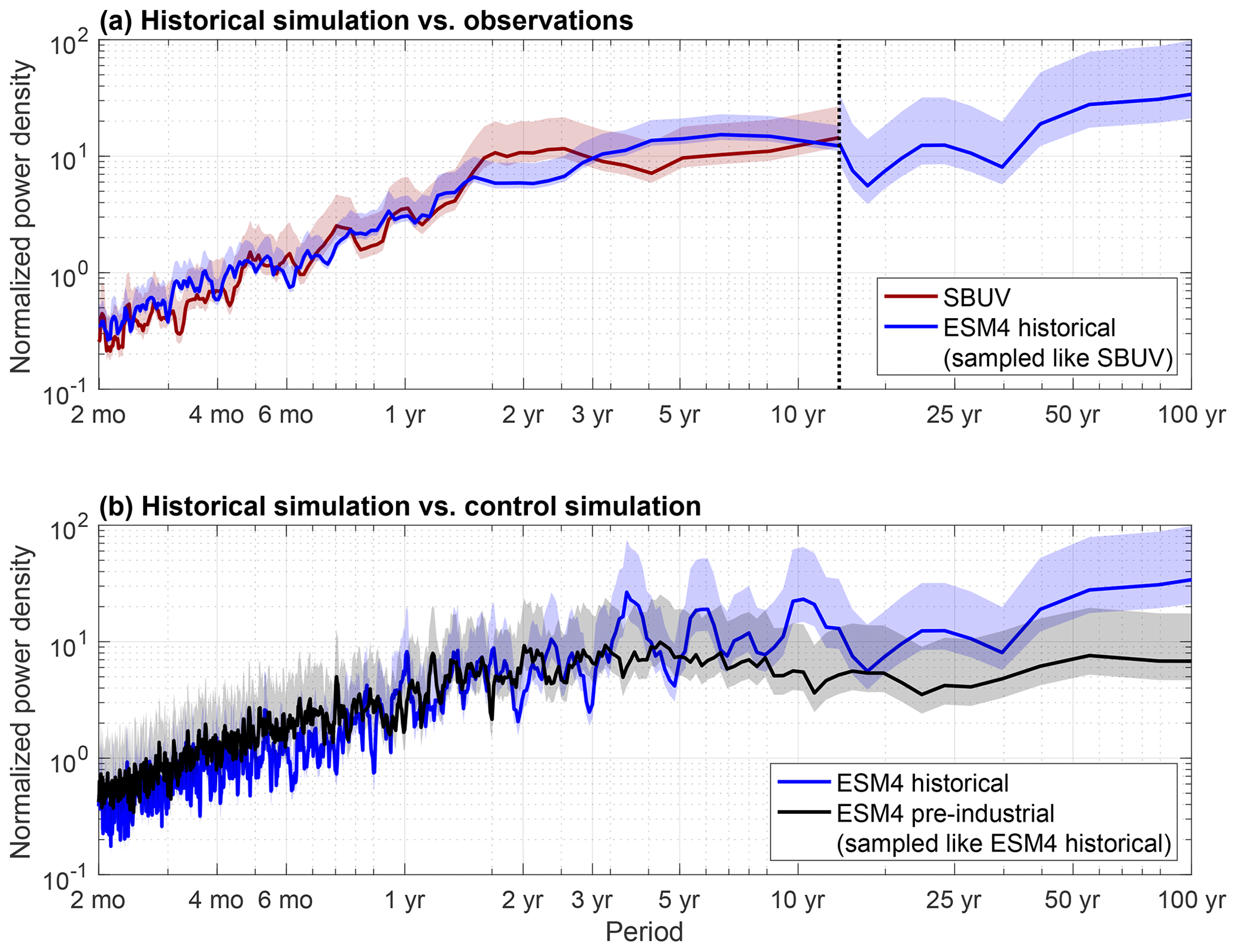
Figure 1 Comparison between observed and simulated normalized variability in the de-seasonalized zonal mean ozone for the 10–16 hPa layer in the Northern Hemisphere midlatitudes (37.5–57.5° N), pictured using power spectral densities (PSDs) estimated with the multitaper method. Shaded areas indicate chi-squared 95 % confidence intervals. To ensure comparability between spectra, the ESM4.1 historical run (1850–2014) is sub-sampled in 13-year periods, matching the longest continuous period given by the SBUV record (dashed line in a), and the resulting power spectra are subsequently averaged. Similarly, in (b), the ESM4.1 pre-industrial run (500 years) is sub-sampled in 165-year periods, corresponding to the length of the historical run. Further, spectral density is normalized by the area under each power spectrum to remove changes in total power.

2.2 Simulations used to estimate trends

We use the average ozone trends from 2000 to 2020 from the same dataset as in Godin-Beekmann et al. (2022): the multi-model mean (16 models) from the CCMI's 1960–2100 period (REF-C2; Eyring et al., 2013b). The purpose of the REF-C2 experiments is to capture future climate trends, and as such, they follow the WMO (2011) A1 scenario for ODSs and the Representative Concentration Pathway (RCP) 6.0 for other greenhouse gas, ozone precursor, and aerosol precursor emissions. Depending on model capabilities, ocean boundary conditions and forcings for the 11-year solar cycle and the QBO are either simulated separately or generated internally. Although the recommendation was not to use volcanic forcings, some models do include them (Godin-Beekmann et al., 2022). More information about the forcings can be found in Eyring et al. (2013a), Hegglin et al. (2016), and Morgenstern et al. (2017). Model runs are accessible at http://catalogue.ceda.ac.uk/uuid/9cc6b94df0f4469d8066d69b5df879d5/ (last access: 7 February 2025) Hegglin et al. (2015).

2.3 SBUV satellite record

The SBUV Merged Ozone Dataset (MOD; version 2 release 1, https://acd-ext.gsfc.nasa.gov/Data_services/merged/, last access: 7 February 2025; see Frith et al., 2014, 2017) combines retrievals from backscattered ultraviolet radiation sensors on board a series of polar-orbiting satellites to provide total column and profile ozone products with monthly frequency. Retrievals include those from first- and second-generation SBUV sensors (algorithm version 8.7) and from the nadir profilers included in the Ozone Mapping and Profiling Suite (OMPS NP, algorithm version 2.8). We use the 2000–2020 portion (21 years) of the MOD (a) to focus on the time period after which the decline in ozone in the upper stratosphere stopped (Newchurch et al., 2003; WMO, 2007), (b) for consistency with other studies, and (c) to avoid issues with coverage gaps in the earlier parts of the record. Indeed, the MOD provides nearly global spatial coverage but suffers from substantial gaps in its temporal coverage. For instance, no reliable measurements are available from April 1976 through November 1978, and there are also none following large volcanic eruptions that injected aerosols in the stratosphere and affected the retrieval (e.g., mid-1991 through 1993; see Bhartia et al., 1993). Early portions of the dataset are also unsuitable for trend analysis due to partial instrument failure (May 1970 to April 1976). Note that among existing merged datasets, the SBUV record provides the densest and most spatially uniform sampling over the 2000–2020 time period (Tummon et al., 2015). Moreover, the MOD record merges data from similar SBUV instruments, and its sampling and retrieval characteristics are more homogeneous over the time period we use than other merged records that rely on more varied data sources.

Both total column and profile ozone products used in this study have a 5° horizontal resolution and are zonally averaged to minimize instrumental uncertainty. The ozone profile product provides ozone amounts in Dobson units (DU) for seven vertical layers spanning the mid-to-upper stratosphere, with layer edges near $\mathrm{25},\mathrm{16},\mathrm{10},\mathrm{6.4},\mathrm{4},\mathrm{2.5},\mathrm{1.6}$, and 1 hPa or approximately $\mathrm{23},\mathrm{27},\mathrm{31},\mathrm{35},\mathrm{40},\mathrm{46},\mathrm{50}$, and 54 km near the Equator (i.e., 4–6 km resolution, which is comparable to that of other nadir-viewing instruments). Data across these layers have accuracy suitable for long-term trend analysis and compare well with ozone records from other spaceborne and ground-based instruments (within 5 %; Bhartia et al., 2013; McPeters et al., 2013). Data outside the 25–1 hPa range tend to be heavily influenced by the a priori ozone climatology used in the retrieval algorithm (Bhartia et al., 1996) and are therefore not relevant to this analysis (see Methods section). Total column ozone data lie within 1 % of the ground-based instrumental record (McPeters et al., 2013).

2.4 Merged satellite trend estimates

We use trend estimates from the ninth report from the initiative on Stratosphere–Troposphere Processes and their Role in Climate (SPARC) on Long-term Ozone Trends and Uncertainties in the Stratosphere (LOTUS; Petropavlovskikh et al., 2019) to provide context for trends derived using the SBUV record alone. The homogenized satellite record used in the LOTUS report includes six merged datasets:

• two that rely on nadir-viewing instruments with relatively broad averaging kernels and low vertical resolution: the SBUV MOD (v8.6, Frith et al., 2014) and the SBUV cohesive dataset from NOAA, and

• four that rely on limb-viewing instruments and occultation techniques characterized by relatively narrow averaging kernels and high vertical resolution: the Global OZone Chemistry And Related trace gas Data records for the Stratosphere (GOZCARDS v2.20, Froidevaux et al., 2015), the Stratospheric Water and Ozone Satellite Homogenized database (SWOOSH v2.6, Davis et al., 2016), the SAGE-OSIRIS-OMPS dataset corrected for sampling effects (corr-SAGE-OSIRIS-OMPS, Damadeo et al., 2018), and the SAGE-CCI-OMPS dataset from ESA (Sofieva et al., 2017).

The LOTUS trend estimates are based on multilinear regression and include proxies to correct for the effects of a range of known climate oscillations (El Niño–Southern Oscillation (ENSO), the QBO, the 11-year solar cycle, the Arctic and Antarctic Oscillations, the North Atlantic Oscillation), as well as changes in the stratospheric meridional circulation, tropopause height, stratospheric sulfate aerosol abundances, and long-term trends in chemically reactive halogens (Steinbrecht et al., 2017). A comprehensive list of references for these proxies is provided in the LOTUS report (Petropavlovskikh et al., 2019). Trends are calculated as the unweighted average of trends from each of the six merged datasets. Trend uncertainties account for the degree of dependency between the datasets and the propagation of errors in the regression model (see Sect. 5.3.2 in Petropavlovskikh et al., 2019). In this study, we use trend estimates for the 2000–2020 period, shown in Figs. 8 and 9 for three broad latitude bands.

3 Methods

3.1 Synthetic SBUV observations for the pre-industrial era

In order to quantify the impact of satellite averaging kernels on the observed variability in stratospheric ozone, we create synthetic observations by applying the SBUV kernels to the ESM4.1 pre-industrial control run. As discussed in the previous section, the model run itself is used as a reference, and the “kernelized” run is used as equivalent observations of the atmosphere had satellites equipped with SBUV sensors flown during the pre-industrial era.

3.1.1 Averaging kernels for synthetic observations

Ozone profiles retrieved by remote sensing are not perfect measurements of the ozone concentrations in each layer of the atmosphere with independent errors but are rather best estimates made given measured radiances and some prior knowledge about the state of the atmosphere. Retrievals are an estimate of some smoothed function of the actual state, with errors that are correlated between different altitudes. As described in Rodgers (1990, 2000), the ozone profile $\widehat{x}$ that is retrieved is related to the true ozone profile x and an a priori profile x_a used in its retrieval by

$$\widehat{x}-x_{\mathrm{a}}=A(x-x_{\mathrm{a}})+{\mathit{ϵ}}_x,$$

where A is the averaging kernel matrix, and ϵ_x represents random and systematic measurement errors. The ith row of A describes where in the column the information attributed to the ith vertical level actually comes from. Thus, averaging kernels are peaked functions whose half-widths correspond to the vertical resolution of the retrieval. Two examples for SBUV are shown in Fig. 2 (also see Fig. 2 in Kramarova et al., 2013a, for more examples). The blue line shows the row of the kernel matrix that corresponds to the 10.1–6.4 hPa layer, and the red line shows the same for the 101.3–63.9 hPa layer. The averaging kernel for the upper level has a peak at the target level, so the concentration attributed to the 10.1–6.4 hPa layer is the weighted average of concentrations between about 2 and 25 hPa but with the largest weight at the target level. The averaging kernel that is intended to represent the 101.3–63.9 hPa layer has a peak around 50 hPa and exhibits large sensitivity to tropospheric ozone, as discussed in Bhartia et al. (2012). Visualizing the kernels helps to demonstrate the limits of SBUV ozone retrievals in the lower stratosphere compared to the middle to upper stratosphere; for vertical levels below 25 hPa, averaging kernels have broad peaks that are significantly shifted away from their respective target levels, indicating that the retrieval for those levels heavily relies on a priori information (Rodgers, 2000). For this reason, as stated in Sect. 2, the analysis with SBUV is limited to pressure levels 25.45 hPa through 1.013 hPa (levels 9 through 15 in the MOD files) and to the total column. Kernel matrices are produced for each retrieval but are only available as monthly averages. We use the monthly averaged kernels for 1 representative year, chosen to be 2005. For simplicity and to reduce the computational cost of the study, we only use the SBUV kernels, even though the MOD record includes OMPS retrievals; note that MOD relies at least in part on SBUV until March 2018.

A priori information typically consists of a climatology obtained via independent measurements. For instance, a priori states for the SBUV merged dataset come from a combination of independent satellite retrievals and reanalysis data validated by comparison with balloon-borne ozonesondes from the Southern Hemisphere ADditional OZonesondes (SHADOZ) network (Ziemke et al., 2021). However, no such independent climatology exists when it comes to creating synthetic retrievals using a pre-industrial model run. Synthetic a priori information is therefore created using the model monthly mean state itself; that is to say, the averaging kernels are applied to the departure of the model state from its monthly climatology. The synthetic a priori is therefore unbiased by construction, and the synthetic retrievals represent a best-case scenario. As a consequence, variability in the synthetic retrievals may be underestimated, but this approach has the added benefit of isolating the effects of the SBUV kernels on the retrieved variability in stratospheric ozone from any effect of the a priori. The relationship between the synthetic retrieval and the simulated ozone (the reference or “true” quantity) is written as

$$\widehat{x}=\stackrel{\mathrm{‾}}{x}+A(x-\stackrel{\mathrm{‾}}{x})+{\mathit{ϵ}}_x,$$

where $\stackrel{\mathrm{‾}}{x}$ denotes the monthly averaged zonal mean simulated ozone profile. As in Rodgers and Connor (2003), the simulated ozone profile is first interpolated onto the coarser SBUV vertical grid so that it can be convolved with the SBUV averaging kernel matrix to produce synthetic retrievals. While the vertical interpolation leads to a loss of some of the higher-resolution information from the model, it is necessary in order to isolate the effects of the averaging kernels, which are illustrated in Fig. 2. The synthetic profile appears smoother than the true profile (hence the expression “smoothing” errors) and is closer to the a priori than the true profile is. Below 25 hPa in the lower stratosphere, the averaging kernels become broader and the retrieval's quality degrades accordingly, hindering the accurate retrieval of large vertical gradients in ozone concentration. Note that the SBUV kernels are not defined during polar night, which means that the synthetic SBUV data effectively capture the seasonal dependence of the SBUV sampling.

Figure 2 (a) Two rows of the averaging kernel matrix and their corresponding SBUV layers (see legend) for 47.5° N in July 2005, normalized using the SBUV a priori as in Kramarova et al. (2013a) (their Eq. 3). (b) One example of a model profile and its synthetic SBUV counterpart for the same time and location, shown as deviations from the model a priori profile to emphasize vertical structures; in this case, maximum deviations are on the order of 1 % of the a priori above (i.e., at pressures lower than) 25 hPa, where the a priori profile peaks, and 1 %–10 % below. The model profile is interpolated onto the SBUV vertical grid to isolate the effects of the averaging kernels.

3.1.2 Consideration of known sources of errors

Random errors (e.g., instrumental noise) in retrieved SBUV profiles are on the order of 1 % (Natalya A. Kramarova, personal communication, 26 January 2023), but since retrievals are averaged zonally and monthly across ∼ 1000 profiles, random errors in the MOD product are neglected, consistent with Kramarova et al. (2013b). This substantial sample size also allows us to ignore the effects of the spatial sampling of SBUV platforms: monthly zonal means in the pre-industrial model are equated with monthly zonal means in the SBUV dataset.

Several non-random error sources in ϵ_x produce latitude- and month-dependent biases; these include errors in a priori profiles as well as calibration-related errors in atmospheric attenuation estimates (N values; see Bhartia et al., 2013). However, errors that normally affect a priori states are not relevant to this study since the a priori states are known with certainty (see Sect. 3.1.1). In addition, since we analyze decadal trends, data are de-seasonalized, and calibration errors that normally affect the seasonal cycle can thus be ignored. Other more sporadic sources of errors, including polar mesospheric clouds, volcanic aerosols, ash, and smoke, are also neglected. Accounting for errors resulting from the merging of different SBUV records and biases from non-uniform temporal sampling (orbital drift) is also challenging because of the nature of our analysis. Therefore, such errors are also neglected.

Given these considerations, the error term ϵ_x is considered negligible. What differs between the synthetic retrievals and the simulated ozone is their respective evolution over the course of the 500 years of simulation – any differences being attributable to the averaging kernels. The impact of these differences on ozone variability is shown in Fig. 3: decadal to multidecadal variability is misrepresented throughout the upper and middle stratosphere, with errors in integrated power frequently exceeding 25 % and occasionally approaching or exceeding 100 %. Unless these errors are explicitly accounted for, they will affect the apparent variability around SBUV trend estimates, and by extension the degree of statistical significance associated with those trend estimates in a general signal-to-noise-ratio sense. Regions in blue indicate where the statistical significance of trends will be overestimated since internal variability is underrepresented there. Regions in red indicate where statistical significance is underestimated; for instance, between 0 and 2.5° N in the 16.4–10 hPa layer, the variability around trends is inflated because the averaging kernels assign variability from adjacent layers (see Fig. 5a) to this layer.

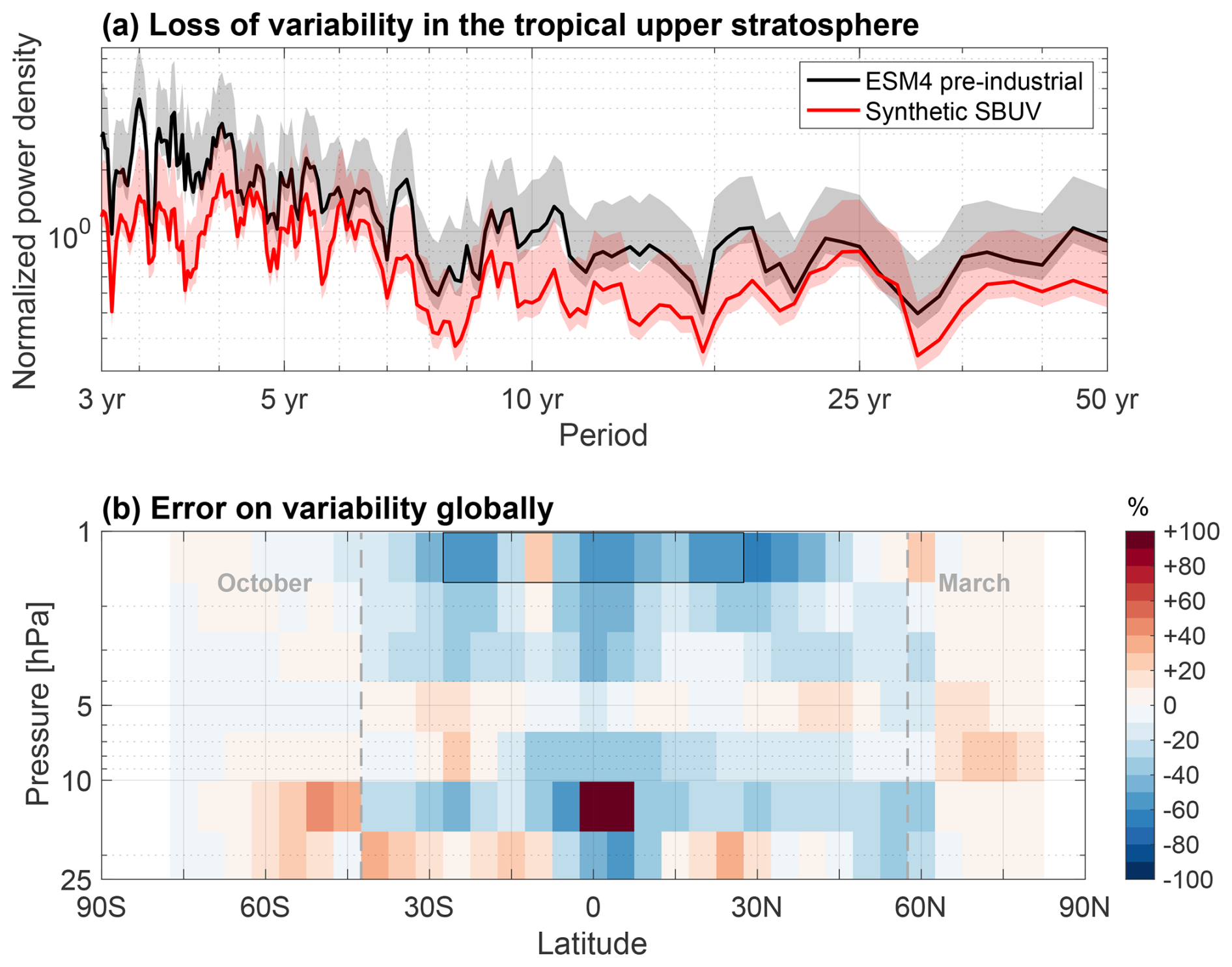
Figure 3 Effect of the SBUV averaging kernels on decadal to multidecadal ozone variability visualized (a) locally for the topmost SBUV layer, 1.6–1 hPa, between 27.5° S and 27.5° N (see the black box in panel b), and (b) globally, as the percent relative error in integrated power density between the pre-industrial run and the synthetic SBUV time series for periods of 10–60 years. Results for only October or March are shown in the high-latitude regions where SBUV data are not available year-round.

3.1.3 Removal of known modes of variability

As in other studies (e.g., Steinbrecht et al., 2017; Petropavlovskikh et al., 2019), an attempt is made to remove the contributions of known modes of variability to the time series of ozone in order to better isolate the internal variability. Several known modes of variability are frequently considered: the seasonal cycle, ENSO, and the QBO on interannual timescales and the solar cycle of irradiance on decadal timescales. Solar irradiance is constant in the pre-industrial run, so no removal of that variability is needed. The seasonal component of variability is modeled as the long-term average ozone abundance for each month of the year and is subsequently removed. The Arctic, Antarctic, and North Atlantic Oscillations were found to have negligible impacts on trends (Petropavlovskikh et al., 2019) and are therefore ignored. Remaining ozone variations are then modeled using the following regression model, similar to that used by Stolarski et al. (1991):

$$\mathrm{\Delta }{\mathrm{O}}_{\mathrm{3}}\left(t\right)=\mathit{\alpha }{\text{QBO}}_{\mathrm{1}}\left(t\right)+\mathit{\beta }{\text{QBO}}_{\mathrm{2}}\left(t\right)+\mathit{\gamma }\text{ENSO}\left(t\right)+\mathit{ϵ}\left(t\right),$$

where α, β, and γ are parameters determined using regression analysis. Unexplained ozone variability is represented by ϵ(t). QBO₁(t) and QBO₂(t) are the two leading empirical orthogonal functions (EOFs) of the de-seasonalized zonal mean monthly zonal wind between 10 and 70 hPa from the model simulations (see Fig. A1), as in Wallace et al. (1993). Following Oman et al. (2013), ENSO(t) is based on the NOAA Oceanic Niño Index (ONI) and captures variations in (modeled) sea surface temperature in the Niño 3.4 region (5° S–5° N, 170–120° W) in the central Pacific Ocean, lagged by 2 months as in Randel et al. (2009). In the pre-industrial model run, QBO₁(t) and QBO₂(t) account for 68 % of the normalized variance of the zonal wind time series. By construction, the correlation between the two EOFs is exactly zero. Thanks in part to the substantial length of the pre-industrial run, the correlation between the QBO EOFs and ENSO(t) is very small (less than 0.05), yielding virtually independent regression terms.

The zonal wind data in Fig. A1 clearly show that the model's internally generated QBO is far from realistic: the weak QBO-like signal is confined to lower pressures, is much more prone to disruption, propagates vertically at more variable rates, and exhibits higher frequencies than the observed QBO. Given these differences, the appropriateness of the traditional EOF-based QBO removal could be called into question, but the model does produce a semi-periodic downward-propagating signal reminiscent of the QBO. Such signals produce large retrieval errors (1 %–6 % in observations) when convolved with the averaging kernels (Kramarova et al., 2013a). Since errors of this nature are the focus of this study, we use the traditional EOF-based approach to removing QBO variability. The QBO removal is performed after the simulated ozone is convolved with the SBUV averaging kernels, to mimic the residual errors produced by the removal of the QBO in SBUV observations.

While the use of EOFs allows us to account for variability due to changes in the amplitude and phase of zonal wind oscillations, it does not account for variability due to changes in the frequency of the oscillations. This is slightly problematic for the removal of the QBO signal in ozone since its frequencies differ between the Equator (where the EOFs are extracted) and higher latitudes (Tung and Yang, 1994). Nevertheless, the average contribution of the QBO to near-equatorial ozone variability is estimated to be about 0.5 % in the model (much smaller than the estimated 10 %–20 % in observations; see Brunner et al., 2006) and is expected to be even smaller at extratropical latitudes, where the atmospheric jets produce large variability. The EOF-based removal of QBO variability is therefore considered sufficient for the purposes of this study.

The methods discussed in this section provide a set of synthetic SBUV data in the absence of anthropogenic forcings and without known climate oscillations. We use this synthetic record to quantify the internal variability in the climate system relevant to stratospheric ozone, so as to estimate the lead time required for long-term trends in ozone to emerge in observations against the backdrop of internal variability. For simplicity, we assume that the modern climate system produces the same internal variability as that during the pre-industrial era. However, while this assumption has been widely used in the analysis of climate model output (e.g., IPCC, 2001; Hegerl et al., 2007; Deser et al., 2012), evidence showing that it may not hold for some variables in climate models exists (e.g., Schär et al., 2004; Scherrer et al., 2005; Rodgers et al., 2021), although different models exhibit different responses in their internal variability under forced change (Maher et al., 2021). Therefore, we suggest caution in interpreting statistical confidence.

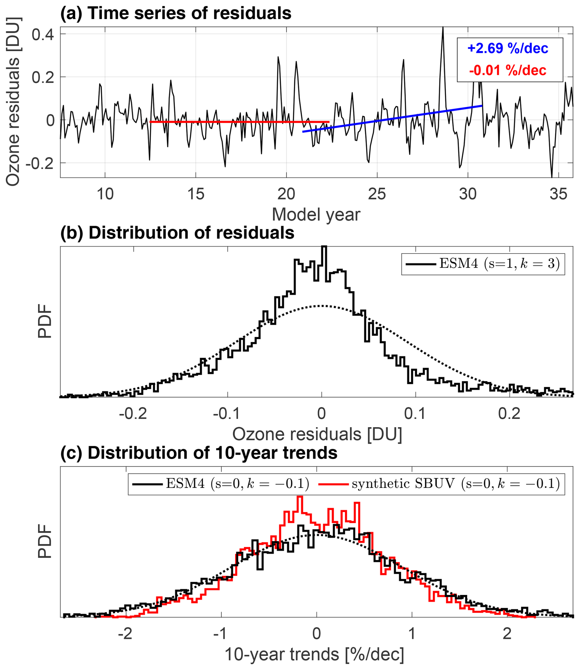
Figure 4 (a) Sample time series of pre-industrial ozone residuals at 2.5–1.6 hPa, 42.5° S, with 10-year trend examples calculated in percent of the mean ozone value at that location, ∼ 4.5 DU. (b) Distribution of ozone residuals for the 500 years of pre-industrial simulation and (c) the corresponding reference distribution of 10-year unforced trends. Dashed lines show Gaussian distributions with moments identical to those from the model distributions for reference. The skewness and excess kurtosis of the distributions are provided in the legend.

3.2 Time of emergence of linear trends

Generally speaking, the smaller the trend, the longer it takes to become distinguishable from background noise. Several methods have been employed in the past to calculate the time of emergence of linear trends. Emergence has sometimes been said to occur when the ratio of the signal (trend) to the noise (internal variability) is large or exceeds a pre-determined threshold (Madden and Ramanathan, 1980; Wigley and Jones, 1981; Giorgi and Bi, 2009; Hawkins and Sutton, 2012). Such methods do not provide the formalism needed for a measure of statistical confidence that links the robustness of the results to the choice of the threshold to exceed. Another method (Mahlstein et al., 2011) defines the time of emergence as that when a statistical test deems an observation unlikely to belong to a distribution that represents an unperturbed climate state. A problem with this method, however, is that it does not account for autocorrelation in the time series, which means that the time of emergence for time series with nonzero autocorrelation is underestimated. Other approaches do take autocorrelation into account; examples include the methods of Tiao et al. (1990), Weatherhead et al. (1998), and Li et al. (2017). In the latter, emergence occurs when a predicted confidence interval of a cumulative trend excludes zero. The confidence interval is described analytically based on the work of Thompson et al. (2015) and accounts for lag-one autocorrelation. However, the method requires the residuals representing internal variability to be normally distributed. This is generally not the case for stratospheric ozone: after removing the seasonal cycle and the contributions from ENSO and the QBO, distributions of residuals often have heavier tails and a narrower peak than a normal distribution (positive excess kurtosis) and are not symmetric (skewness is nonzero; see an example in Fig. 4b).

3.2.1 Definition of the time of emergence

For these reasons, the time of emergence is calculated using the method of Rivoire et al. (2024) (R24 hereafter), which provides nearly identical results to that of Li et al. (2017) but can handle non-normally distributed residuals. R24 found empirical evidence that the method of Li et al. (2017) may still be used when residuals exhibit nonzero skewness or excess kurtosis, but without any formalism to prove this generally, we consider the method of R24 to be a safer choice. The general principle behind the method is to compare a linear trend of interest, denoted b, to a distribution of linear trends that arise purely as a result of internal variability. If b is located near the central quantiles of the reference distribution, then b aligns with typical fluctuations seen in the absence of external forcings. Conversely, if b is located near the outer quantiles, then it is unusually large compared to natural fluctuations and can reasonably be hypothesized to be the result of external forcings.

The reference distribution is calculated by sampling linear trends in the control simulation using a sampling window of fixed length (see Fig. 4a and c). The time of emergence, denoted y, is the length of the sampling window that yields a reference distribution such that $\left|b\right|$ exceeds $c=\frac{c_{\mathrm{d}}+\mathrm{100}}{\mathrm{2}}$ % of unforced trends, with c_d as the statistical confidence threshold for a two-sided test. In the rest of the paper we use c_d=95 % as the threshold for statistical significance. Although the use of this particular threshold is commonplace, we emphasize its arbitrary nature and caution against over-interpreting its significance.

In practice, the time of emergence is determined by iteration, starting with the shortest possible sampling window of two model time steps. The reference distribution of unforced trends over all possible two-step intervals (with overlap) is calculated, and its cth percentile is compared to $\left|b\right|$. The length of the sampling window is then progressively increased until the statistical criterion described above is met. For more details on this technique and its efficient implementation, the reader is referred to Sect. 2 of R24.

Since the time of emergence y is calculated using a trend distribution sampled directly from a model run, it neglects the effects of observational uncertainties. Figure 5 shows this “ideal” time of emergence – which is valid only if one possesses omniscient knowledge of the atmosphere – for both a homogeneous trend and the actual trends from CCMI-1 simulations. R24 shows that observational uncertainties can introduce large errors in y, and they provide the formalism to correct y accordingly. In our case, the correction for y accounts for the effects of the vertical redistribution of ozone variability by the averaging kernels (see Figs. 2 and 3). The corrected time of emergence is denoted y^* and is calculated using reference trend distributions sampled from the synthetic SBUV retrievals introduced earlier (e.g., the red curve in Fig. 4c) rather than the model run itself (the black curve in Fig. 4c). As a result, y^* quantifies the time of emergence of ozone trends as seen by SBUV platforms (see Sect. 4.2 and Fig. 6).

3.2.2 Notes on the realism of the pre-industrial control simulation

Since emergence is defined based on the representation of internal variability from a model, the realism of the model comes into question. On the one hand, the time of emergence y is subject to the realism – or lack thereof – of the model: misrepresentations in the magnitude or frequency spectrum of internal variability yield errors in the time of emergence. Although we provide an analysis of said realism to the extent possible (Sect. 2.1), quantifying these errors is inherently difficult given the absence of pre-industrial references for observed variability. On the other hand, R24 showed that the adjustment for the effect of observational uncertainties on the time of emergence, when expressed as a relative error ($\frac{y^{*}-y}{y}$), is accurate even if the model dramatically misrepresents internal variability. For this reason, we quantify the effect of the SBUV kernels on the time of emergence as a relative error (see Sect. 4.2).

4 Results

4.1 Time of emergence

Figure 5 provides estimates for the time of emergence (y, in years since 2000) with 95 % confidence for both a spatially homogeneous 1 % per decade trend (panel b) and the 2000–2020 trends from CCMI-1 (panel c). To put this into context, panel (a) shows the average ozone abundances and their standard deviation in the pre-industrial run. The spatially homogeneous trend serves to illustrate the effects of internal ozone variability on the time of emergence. Except for the lowermost stratosphere, a general correlation is seen between the time of emergence and ozone variability as quantified by its standard deviation: the largest values are found in the tropical middle-stratosphere and polar regions. Departures from this correlation arise where the spectrum of variability includes non-Gaussian behavior and is not well described by the standard deviation alone.

According to our method and based on ESM4.1 as a reference for internal variability, trends associated with the CCMI-modeled evolution of ozone under the Montreal Protocol may not emerge until the second half of the century in the heart of the midlatitude ozone layer (panel c). In the upper stratosphere (above 10 hPa), chemistry–climate model trends for 2000–2020 are largely distinguishable from ESM4.1's natural variability with ∼ 20 years of model record, in agreement with the previous literature showing significantly increased ozone abundances (Gillett et al., 2011; Arblaster et al., 2014). Lower down, especially in the middle stratosphere (10–30 hPa), our method finds that trends have generally not emerged yet. In the midlatitudes (35–60° N/S), trends may require decades of additional record to emerge, owing in part to large variability and in part to small trends. This finding is generally consistent with the existing literature, which finds little to no significance to trends in the region (WMO, 2022, and references therein). Over the Arctic, we find that the emergence of positive trends could occur by 2030, compared to the literature expecting visible signs of recovery there in the mid-2040s. However, since our results are based on the analysis of a single model, we urge caution: previous analyses have concluded that large dynamical variability in this region precludes the detection of recovery until the late 21st century (WMO, 2022). It is possible that the ozone interannual variability in ESM4.1 still lacks realism despite recent improvements (Horowitz et al., 2020, their Fig. 11).

For vertically integrated ozone (panel d), despite the relatively small variability in the tropical region, emergence occurs later there because trends are small. Trends associated with chemical loss over the polar caps in spring are isolated using October- and March-only time series in the Southern Hemisphere and Northern Hemisphere, respectively. Although ozone loss is largest over Antarctica and is therefore expected to exhibit the clearest signs of recovery (Newchurch et al., 2003; Yang et al., 2008; Charlton-Perez et al., 2010), the analysis predicts that trends for October and March only emerge after ∼ 40 years near the strongest trends (65° N/S, not shown), owing to large variability. Closer to the poles, October and March trends become very small and therefore take much longer to emerge.

Some caveats should be kept in mind: the time of emergence is based on a representation of unforced ozone variability that excludes the effects of ozone-depleting substances or volcanic aerosols (see Fig. 1). As a result, time of emergence estimates provide lower bounds for the timing of the detection of recovery (as long as the linear trend approximation holds). Further, in the previous literature, statistically significant trends associated with the recovery of the ozone layer are based on more than just ozone abundances; they include trends in other metrics, such as the minimum in 15 d average total ozone, maximum in 15 d average 220 DU ozone hole area, minimum in 15 d average ozone mass deficit, and the duration of the ozone hole (e.g., Tully et al., 2020). It is possible that these metrics provide more detectable trends than ozone abundances alone. Lastly, we highlight the fact that quantifying the emergence of a trend vs. that of an epoch difference may yield different results.

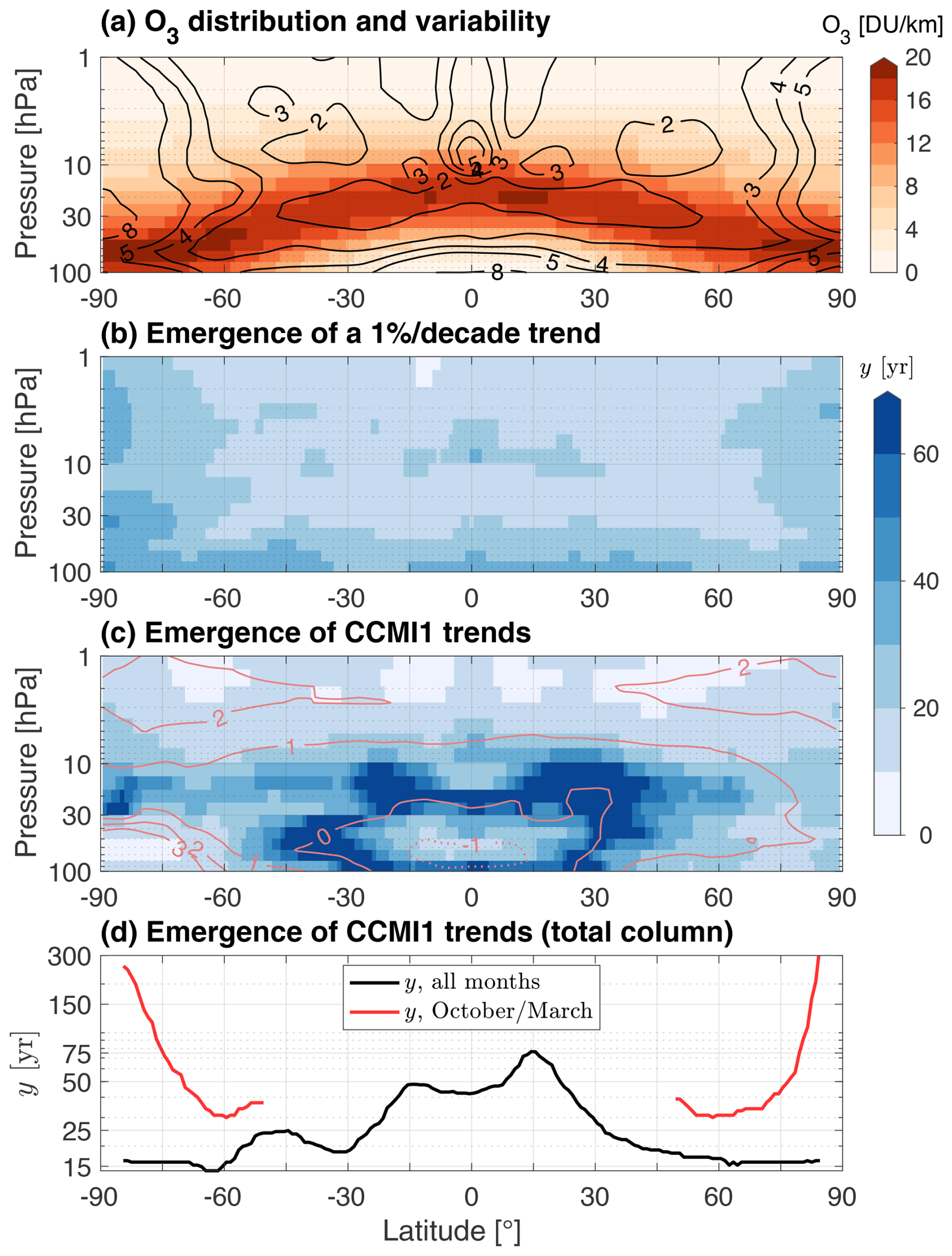
Figure 5 (a) Average ozone abundance in the ESM4.1 pre-industrial run (in DU per km, colors) and relative standard deviation of the de-seasonalized time series (black contours, in percent). (b) Ideal time of emergence (y) for a spatially homogeneous 1 % per decade trend in years, with contours every 10 years. (c) Ideal time of emergence for 2000–2020 trends in CCMI-1 ref-C2 (shown by overlaid red contours, % per decade). (d) Ideal time of emergence (y) for 2000–2020 trends in CCMI-1 ref-C2 total column ozone. Results for October only (March only) are shown in the Southern (Northern) Hemisphere.

4.2 Effect of the SBUV kernels on the time of emergence

Results established so far apply to the “model world” only and do not factor in the limitations of observing platforms that make up the historical record. The synthetic SBUV record from Sect. 3 provides an example of the effect of observational limitations on the time of emergence. Figure 6 shows those limitations as the relative difference between the kernel-adjusted time of emergence y^* and the ideal time of emergence y. Large errors throughout the middle and upper tropical stratosphere are reminiscent of the patterns of variability associated with the QBO despite the prior removal of QBO variability (Sect. 3.1.3). This result arises because the convolution of the SBUV kernels with the ozone data affects the representation of the QBO (Kramarova et al., 2013a) but does not affect the wind field that is used to perform the QBO removal. Other error patterns arise where ozone variability is large, for example across the 16–10.1 hPa layer and above the polar caps (refer to Fig. 5a). The unavailability of SBUV retrievals during polar night may contribute to errors over the polar caps. Interestingly, errors are opposite in sign between the two polar caps at some levels, indicating opposite effects due to the combined SBUV averaging kernels and lack of measurements there. Errors are slightly larger over the southern polar cap than the northern, which is attributable to slightly larger internal variability in ESM4.1 in the Antarctic (as shown in Fig. 5a). This result is more specifically attributable to the shape of the power spectrum of internal variability in ESM4.1 around periods corresponding to the time of emergence. The largest negative errors (i.e., relative differences) found near the Equator just below 10 hPa are explained by the unusual overestimation of internal variability attributable to the SBUV kernels shown in Fig. 3b. At all latitudes, the error pattern is qualitatively unchanged whether trend magnitudes are homogeneous (panel a) or not (panel b), indicating that our method provides generally applicable understanding of the deficiencies of the SBUV ozone retrieval for detecting trends.

For total column ozone, the kernel-adjusted time of emergence estimates are very close to the ideal estimates (Fig. 6c). This is consistent with the result in Kramarova et al. (2013a) (their Fig. 6): combining SBUV layers improves the accuracy of ozone retrievals.

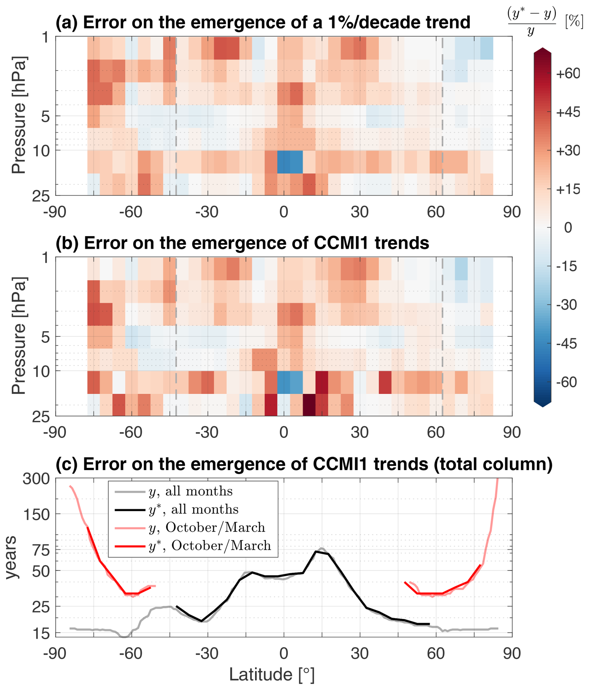
Figure 6 Relative error of the time of emergence due to the SBUV kernels ($\frac{y^{*}-y}{y}$) for (a) a spatially homogeneous 1 % per decade trend and (b) the CCMI-1 trends from panel (c) in Fig. 5. Dashed gray lines denote the latitudes poleward of which the SBUV retrieval is not available year-round. (c) Ideal time of emergence (y) and kernel-adjusted time of emergence (y^*) for 2000–2020 CCMI-1 trends in total column ozone.

4.3 Effect of the SBUV kernels on vertically resolved trend estimates

Retrieval methods based on averaging kernels have previously been said not to affect trend estimates (Petropavlovskikh et al., 2019). The rationale behind this statement is straightforward: since the retrieval process remains unchanged over time, errors attributable to it are also constant over time (at least in a long-term sense), and trend estimates are therefore unbiased. However, this rationale fails to account for the vertical redistribution of information by the kernels. As trends affect the true profile (x in Sect. 3.1.1), the difference between the true profile and the a priori profile (x−x_a) also contains a trend signal. Once the kernel matrix is convolved with (x−x_a), the trend signal is redistributed vertically. As a result, trend estimates at each vertical level are affected by the trend signal from adjacent levels in a manner defined by the shape of the averaging kernels. This is true of any profile, including the hypothetical case of a vertically uniform profile in the context of trends expressed in percent per unit time, but errors can be especially large when trends are vertically heterogeneous. Figure 7 shows such errors for a few idealized trend profiles representing possible ozone increases in the mid-to-upper stratosphere in the northern midlatitudes (Godin-Beekmann et al., 2022; see also Figs. 3–10 in WMO, 2022): one broad maximum and one narrower maximum centered near 2.5 hPa and one maximum centered near 6 hPa. The SBUV kernels attenuate peaks in the idealized trend profiles and shift the maxima to other altitudes above and below the true peaks. Errors as large as 100 % and displacements as large as 6 km are found, highlighting the importance of accounting for the retrieval process in estimating trend uncertainties. Negative correlation coefficients between layers in the averaging kernel matrix can yield negative trends even when the true trends are only positive.

The results suggest that trends in the middle and lower stratosphere may be affected by the presence of trends in the upper stratosphere. This is particularly relevant in the context of analyses that show negative trends in the lower stratosphere (e.g., Ball et al., 2018). While the errors near 25 hPa may seem small, they may induce large errors in the time of emergence. Altogether, this analysis highlights the importance of accounting for satellite averaging kernels when analyzing vertically resolved trends.

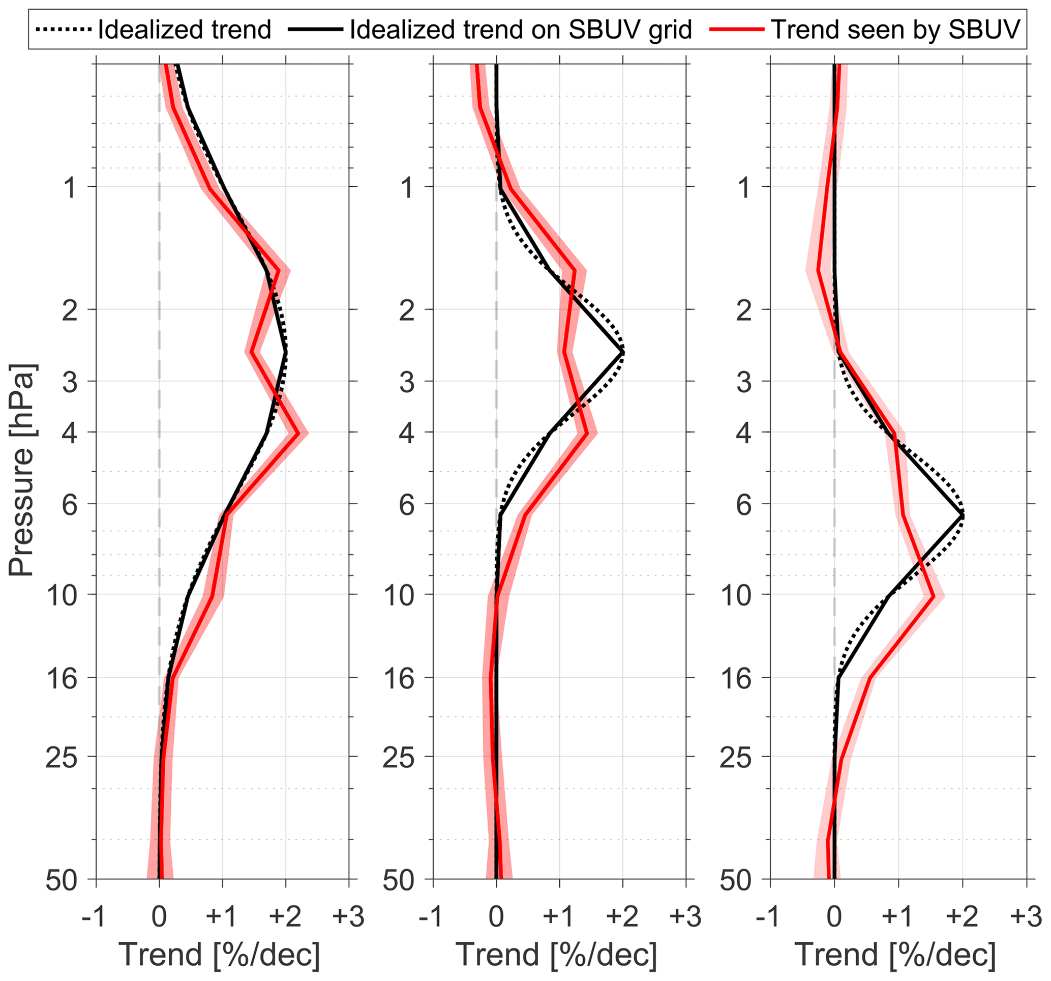
Figure 7 Idealized trend profiles representing three hypothetical scenarios for ozone recovery in the mid-to-upper stratosphere (black) and corresponding profiles that would be observed by SBUV at 42.5° N (red). The red shading shows the interquartile range for trends estimated using 24 years of data (roughly the length of the record since 2000).

4.4 Smallest detectable trends

When trend estimates are in disagreement across model simulations or observational records, the method from R24 can be used to determine the range of trend magnitudes that should be distinguishable from internal variability in the first place. Using the time of emergence y as the length of the sampling window used to calculate trends from the control run (or its synthetic counterpart), b is the smallest detectable trend at confidence level c_d. Trends with a magnitude smaller than $\left|b\right|$ are not distinguishable from internal variability at the chosen degree of confidence. The magnitude of b provides an “envelope of undetectability”, shown in Fig. 8 for a few key latitude bands, assuming omniscient/model knowledge. Simulated and observed 2000–2020 trends in the upper stratosphere (above 10 hPa) largely lie outside the range of undetectable trends, indicating that the trend estimates have emerged from internal variability there. Interestingly, the inter-model spread only lies outside the envelope above 3–5 hPa. Below 10 hPa, mean trends are located within the range of undetectability, which means that the internal variability is so large that 21 years of data is not sufficient to ascertain whether ozone is increasing or decreasing with 95 % certainty there. Further, simulated and observed trends within the heart of the ozone layer (see Fig. 5a) are currently not detectable with 95 % statistical confidence according to the datasets used and again, assuming omniscient knowledge.

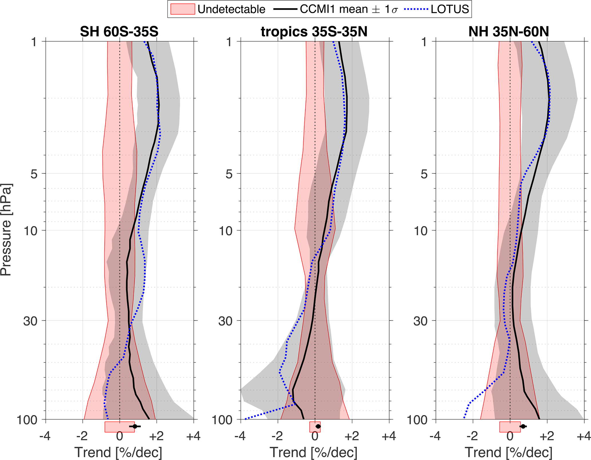
Figure 8 Simulated 2000–2020 ozone trends from CCMI-1 and the corresponding range of undetectable trends at the 95 % confidence level. Results for total column ozone are shown at the bottom outside each panel. Observed 2000–2020 trends from LOTUS are shown in blue for reference.

The same analysis is performed on the synthetic SBUV control simulation to obtain the envelope of undetectability accounting for observational uncertainties. Figure 9 overlays this SBUV envelope and that given by the unaltered model run, that is, the ideal envelope of undetectability (from Fig. 8). Overall, SBUV envelopes are slightly optimistic (i.e., narrower, by a few tenths of a percent per decade) because the SBUV kernels tend to reduce the true internal variability (in the latitude-band-average sense; compare to Fig. 3) or affect its spectrum in a way that artificially decreases the time of emergence. The differences between the true and SBUV envelopes (Fig. 9) are most noticeable in the tropical region, where the SBUV kernels yield errors up to 25 %. Note that averaging the smallest trends over latitude bands reduces the SBUV kernel errors – those can be as large as 50 % locally (not shown). As was concluded from Fig. 6, the detectability of total column ozone trends is virtually unaffected by the SBUV kernels.

The SBUV envelope is most relevant to trends estimated using the SBUV record, and it provides useful context for comparative studies that include SBUV trends (e.g., Frith et al., 2014; Harris et al., 2015; Tummon et al., 2015; Solomon et al., 2016; Chipperfield et al., 2017; Steinbrecht et al., 2017; Weber et al., 2018; Ball et al., 2018; Brönnimann, 2022). We draw a comparison with the LOTUS trends since LOTUS is subject to the limitations of SBUV, among those of other datasets. The results are qualitatively similar to those in Fig. 8: trend estimates above 10 hPa should generally be distinguishable from internal variability, with the caveat that errors from the SBUV kernels can yield moderate overconfidence where trend estimates are close to the smallest detectable trends. Note that the large differences between SBUV-only and LOTUS trends are likely due to the heavy reliance of the LOTUS product on limb sounder retrievals, which have narrower averaging kernel peaks than those shown in Fig. 2, resulting in an ∼ 2.5 km intrinsic vertical resolution in the lower stratosphere (compared to 6 to 10 km for SBUV). Below 10 hPa, most trends are predicted to be indistinguishable from internal variability.

Similar detectability envelopes could be quantified for other nadir sounders, for instance the Global Ozone Monitoring Experiment (GOME; Burrows et al., 1999), Ozone Monitoring Instrument (OMI; Levelt et al., 2006), or Tropospheric Emission Spectrometer (TES; Worden et al., 2004). Limb sounders are subject to similar errors given the extent that they also rely on averaging kernels, for instance OMPS-LP (Arosio et al., 2018), the Optical Spectrograph and Infrared Imager (OSIRIS; von Savigny et al., 2003), Atmospheric Chemistry Experiment Fourier Transform Spectrometer (ACE-FTS; Walker et al., 2005), Michelson Interferometer for Passive Atmospheric Sounding (MIPAS; Ridolfi et al., 2000), Microwave Limb Sounder (MLS; Livesey et al., 2006), and Stratospheric Aerosol and Gas Experiment III (SAGE III; Cisewski et al., 2014). However, since limb sounders typically achieve a much better vertical resolution than nadir sounders, kernel errors are likely to affect the detectability of trends to a lesser extent.

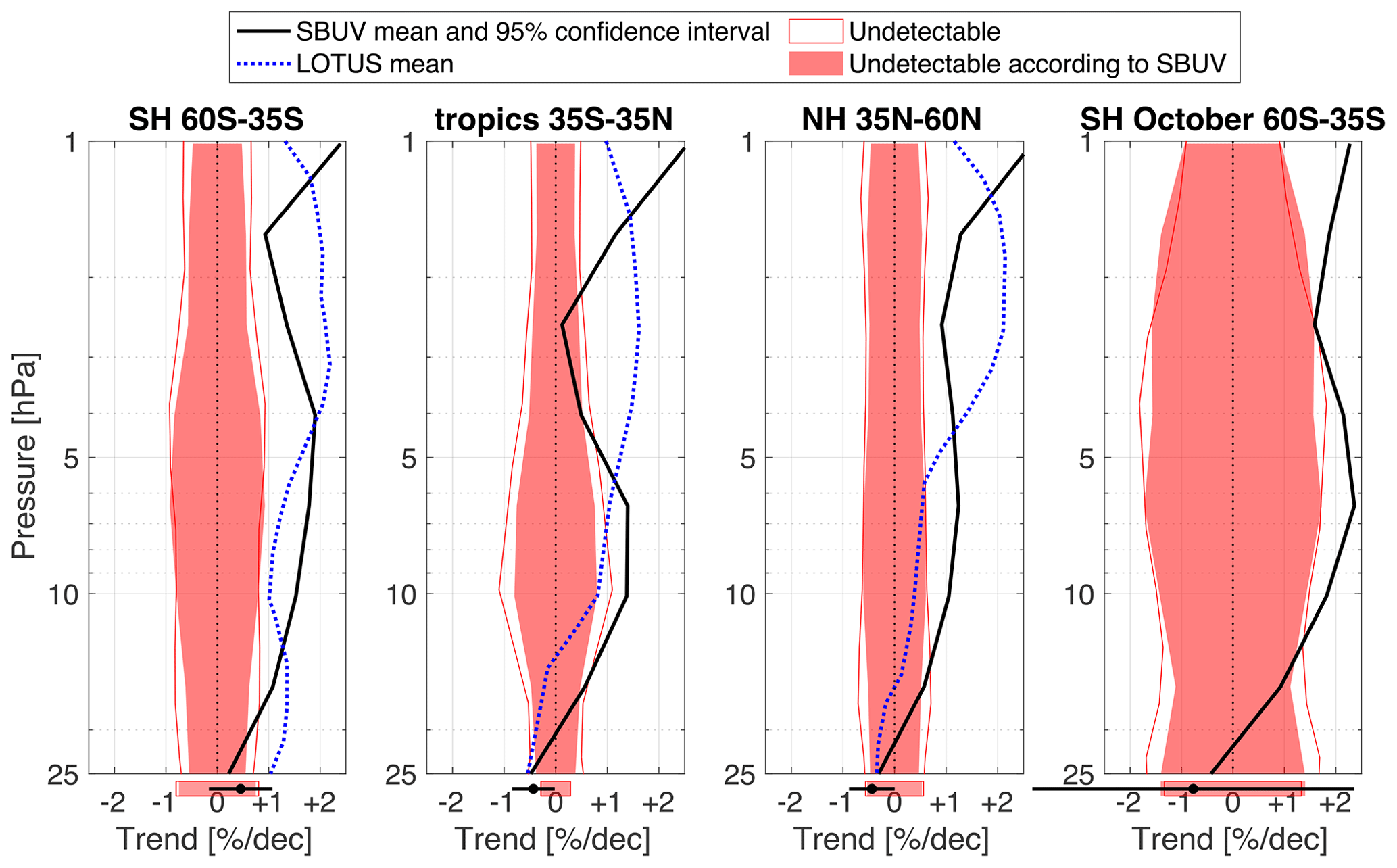
Figure 9 SBUV 2000–2020 ozone trends and the corresponding envelope of undetectability at the 95 % confidence level, including the adjustment for SBUV kernels, which tend to yield slightly narrower envelopes. Results for total column ozone are shown at the bottom outside each panel. Observed 2000–2020 trends from LOTUS are shown in blue for reference. The confidence interval around SBUV trends comes from linear regression coefficient estimates.

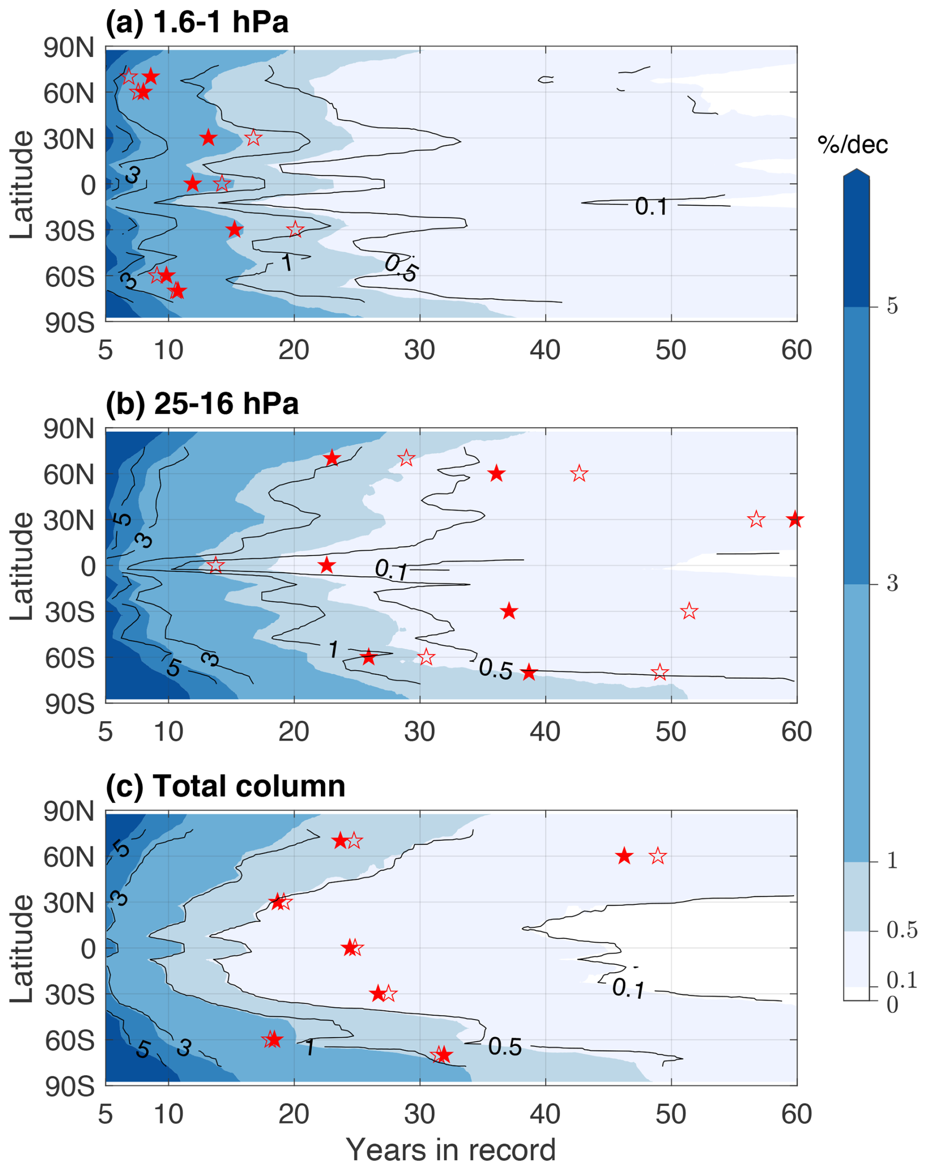
Figure 10 The smallest detectable ESM4.1 pre-industrial trends at the 95 % confidence level (shaded) and their SBUV kernel-adjusted counterparts (black contours) given as a function of the length of the available record for (a) 1.6–1 hPa, (b) 25–16 hPa, and (c) the total column. Filled and unfilled red stars indicate the emergence of CCMI-1 2000–2020 trends at a few latitudes based on the ESM4.1 smallest detectable trends and their SBUV kernel-adjusted counterparts, respectively.

The results discussed here raise the following question: if not now, when will trend estimates eventually become distinguishable from internal variability? To answer this question, Fig. 10 shows the magnitude of the smallest detectable trends as a function of the length of the record. In the upper stratosphere (∼ 1 hPa, Fig. 10a) where CCMI-1 trend estimates are 1 % per decade–2 % per decade, the current length of record since 2000 is sufficient to rule out the possibility that the observed increase in ozone is an artifact of internal variability, even when accounting for SBUV kernel errors. This result is in agreement with Fig. 5c and arises despite the relatively large underestimation of internal variability shown between 60° S and 60° N in Fig. 3b. Lower down (25–16 hPa, Fig. 10b), CCMI-1 trends are about a factor of 2 smaller, and ozone variability is larger; therefore, much longer records are needed. In the Northern Hemisphere midlatitudes, 35 to 60 years of record are needed. Over the southern polar cap, almost 40 years of data are needed, increasing to 50–60 years when accounting for SBUV kernel errors. In contrast, the SBUV kernels yield overestimated internal variability near the Equator (Fig. 3b), and accounting for such errors therefore decreases the length of the record needed to detect the CCMI-1 trend estimate (the unfilled red star is shifted toward earlier years than the filled one). For total column ozone (Fig. 10c), the results suggest that CCMI-1 trends have emerged or will soon, except in the Northern Hemisphere midlatitudes and over Antarctica. SBUV kernel errors have little effect on these estimates, consistent with previous findings (Kramarova et al., 2013a). We emphasize that these results are based on the analysis of a single model (ESM4.1) and that the definition of emergence used here differs from typical measures of statistical significance based on the standard error in regression coefficients. These caveats are important to keep in mind, given that observational studies have found signs of recovery in some column ozone metrics above Antarctica (WMO, 2022, Chap. 4).

5 Conclusions

We examined the statistical significance of long-term trends in stratospheric ozone. Statistical significance was tested against the null hypothesis of no forced change rather than the null hypothesis of no change, in order to include information about the magnitude of trends that arise purely as a result of internal variability in the climate system. Using the concept of time of emergence, we showed the potential for large errors in the statistical significance of trends estimated from satellite records: trends may appear to emerge from internal variability when in fact they are not robust and will require several more years to decades of observations to emerge. Two factors explain these results: (1) the averaging kernels inherent to the optimal estimation retrieval technique consistently misrepresent decadal to multidecadal variability in nadir-viewing satellite observations, and (2) known modes of variability (ENSO, QBO) interact with averaging kernels, and their removal from the observed record is therefore prone to residual errors.

Further, our analysis showed that by vertically redistributing information, averaging kernels can alter trend magnitudes, in addition to their uncertainties. This result contrasts with the assumption of Petropavlovskikh et al. (2019), who stated that kernels do not affect trends since kernel errors are constant in time. We find instead that the shape of the vertical trend profile is subject to large errors: hypothetical scenarios of ozone recovery at a rate of 2 % per decade in the mid-to-upper stratosphere yield errors up to 1 % per decade, with possible vertical displacements in the altitude of local maxima of up to 6 km, consistent with Fig. 3-10 in WMO (2022). We also find errors in the sign of trends, with location and magnitude depending on the hypothetical profile used. Our analysis uses SBUV as an example, but other nadir sounders (e.g., GOME, OMI, TES) are in principle subject to similar effects, with magnitude dependent on their vertical resolution and the location of their vertical levels relative to vertical gradients in ozone concentrations and variability. Limb sounders (e.g., MLS, OMPS-LP, OSIRIS, ACE-FTS, MIPAS, SAGE III) may also be affected, albeit to a lesser extent.

We note a few caveats to our study. Time of emergence estimates are subject to the realism of the model we used (ESM4.1), although the relative adjustment to the time of emergence remains accurate. The reference simulation we used excludes the influence of volcanoes, which can be large. Additionally, the effects of non-uniform sampling and record-merging procedures are also excluded. The time of emergence estimates presented here should therefore be construed as lower bounds (as far as linear trends are concerned). Our time of emergence values may be further underestimated if the internal variability in the climate system is increasing under forced change (as discussed by Rodgers et al., 2021). In addition, we used an arbitrary 95 % threshold for statistical significance, and quantitative results are of course sensitive to this choice. Lastly, in this study we did not explore derived metrics related to ozone recovery (e.g., size and timing of the ozone hole; WMO, 2022, Chap. 4, Sect. 4.4.2.1), which may confer different detection power with respect to long-term trends.

Our results should be interpreted with these caveats in mind, but nonetheless, they provide useful context in light of the varying degrees of confidence placed in trends in the recent literature; notably, adding just a few years to the historical record can change the magnitude and even the sign of trends in some locations. Based on our results, we recommend systematically accounting for the effects of averaging kernels when calculating long-term trends using vertically resolved ozone records, particularly those from nadir-viewing instruments. We further recommend testing the statistical significance of trends against the null hypothesis of no forced change rather than no change at all. Future work in this direction would benefit from long reference simulations of chemistry–climate models with perpetual year-2000 conditions, to better characterize the variability relevant to the recovery of the ozone layer since then.

Appendix A: Representation of the QBO in the pre-industrial simulation

Figure A1 highlights differences between the QBO generated internally by the ESM4.1 pre-industrial model run and the observed QBO (see discussion in Sect. 3.1.3).

Figure A1 Sample time series of the simulated (a) and observed (b) de-seasonalized monthly zonal mean zonal wind. Positive values denote westerly wind anomalies.