the Creative Commons Attribution 4.0 License.
the Creative Commons Attribution 4.0 License.
 | 20 Jun 2023
Change from aerosol-driven to cloud-feedback-driven trend in short-wave radiative flux over the North Atlantic
Daniel P. Grosvenor
Kenneth S. Carslaw
Aerosol radiative forcing and cloud–climate feedbacks each have a large effect on climate, mainly through modification of solar short-wave radiative fluxes. Here we determine what causes the long-term trends in the upwelling short-wave (SW) top-of-the-atmosphere (TOA) fluxes (FSW↑) over the North Atlantic region. Coupled atmosphere–ocean simulations from the UK Earth System Model (UKESM1) and the Hadley Centre General Environment Model (HadGEM3-GC3.1) show a positive FSW↑ trend between 1850 and 1970 (increasing SW reflection) and a negative trend between 1970 and 2014. We find that the 1850–1970 positive FSW↑ trend is mainly driven by an increase in cloud droplet number concentration due to increases in aerosol, while the 1970–2014 trend is mainly driven by a decrease in cloud fraction, which we attribute mainly to cloud feedbacks caused by greenhouse gas-induced warming. In the 1850–1970 period, aerosol-induced cooling and greenhouse gas warming roughly counteract each other, so the temperature-driven cloud feedback effect on the FSW↑ trend is weak (contributing to only 23 % of the ΔFSW↑), and aerosol forcing is the dominant effect (77 % of ΔFSW↑). However, in the 1970–2014 period the warming from greenhouse gases intensifies, and the cooling from aerosol radiative forcing reduces, resulting in a large overall warming and a reduction in FSW↑ that is mainly driven by cloud feedbacks (87 % of ΔFSW↑). The results suggest that it is difficult to use satellite observations in the post-1970 period to evaluate and constrain the magnitude of the aerosol–cloud interaction forcing but that cloud feedbacks might be evaluated.
Comparisons with observations between 1985 and 2014 show that the simulated reduction in FSW↑ and the increase in temperature are too strong. However, the temperature discrepancy can account for only part of the FSW↑ discrepancy given the estimated model feedback strength (). The remaining discrepancy suggests a model bias in either λ or in the strength of the aerosol forcing (aerosols are reducing during this time period) to explain the too-strong decrease in FSW↑, with a λ bias being the most likely. Both of these biases would also tend to cause too-large an increase in temperature over the 1985–2014 period, which would be consistent with the sign of the model temperature bias reported here. Either of these model biases would have important implications for future climate projections using these models.
- Article
(11387 KB) - Full-text XML
- BibTeX
- EndNote


Many changes have occurred over the historical period, 1850–2014: the industrial revolution, during which North America and Europe in particular emitted increasing amounts of greenhouse gases, aerosols, and aerosol precursors; the introduction of clean air acts by North America and Europe starting in the 1950s that led to reduced aerosol emissions from those regions; the industrialization of China and India leading to increased emissions of greenhouse gases and aerosols; and the general continued rise in the rate of global greenhouse gas emissions. Climate change over the North Atlantic (NA) on decadal and longer timescales is influenced by many different factors, with the most significant likely being greenhouse gas forcing, aerosol forcing, mid-latitude cloud feedbacks mediated by temperature changes, natural variability and the Atlantic Meridional Overturning Circulation (AMOC). Many of the processes involve changes in the upwelling short-wave (SW) radiative flux at the top of the atmosphere (FSW↑); therefore, FSW↑ is a key property of the Earth system when considering climate variability.
Fairly long-term observational records of FSW↑ exist for the recent part of the historical period (e.g. 1985–2019; Allan et al., 2014a; Liu et al., 2015, 2017a) that may be useful for evaluating models and attributing changes in climate to various causes. However, to understand what model evaluation using such long-term datasets is telling us about the causes of regional climate change, it is necessary to understand the driving factors of long-term changes in FSW↑. In this study we use the UK Met Office climate models to better understand the underlying processes and what the observed long-term trends in FSW↑ might be telling us about model performance and causes of regional climate change.
We focus on the NA region, because it plays a major role in several aspects of the Earth system. The NA ocean sequesters large amounts of carbon and heat from the atmosphere and therefore helps to regulate the global climate (Buckley and Marshall, 2016). Processes in the NA are thought to help determine the speed of the AMOC (Buckley and Marshall, 2016), which transports a significant amount of heat northwards, representing ∼ 25 % of the total (atmospheric plus oceanic) global northward heat transport at 24–26∘ N (Srokosz et al., 2012). The AMOC transports a large amount of energy from the Southern Hemisphere to the Northern Hemisphere, something that is not true for the equivalent circulations in the Pacific (Buckley and Marshall, 2016). This cross-equatorial oceanic heat flow is important, because it leads to a compensating southward cross-Equator heat flow within the atmosphere, and this in turn causes the Intertropical Convergence Zone (ITCZ) to be positioned north of the Equator. Changes in the AMOC can therefore lead to changes in the ITCZ position, which could bring great disruption to the climate of not only the Atlantic region but also the climates of the global tropics, subtropics and potentially the midlatitudes via changes in precipitation and changes to the Indian and Asian monsoons (Buckley and Marshall, 2016; Chiang and Friedman, 2012; Srokosz et al., 2012).
The NA is surrounded by North and Central America, Europe, and North Africa, which are large regions of high population density. This means that (1) there is a great deal of influence from short-lived anthropogenic species such as aerosols over the NA and (2) that changes in the NA climate system can have large impacts on human society. Sea surface temperature (SST) variability in the NA has been associated with impacts on important phenomena such as tropical storm and hurricane activity (Zhang and Delworth, 2006; Smith et al., 2010; Dunstone et al., 2013); anomalies in rainfall in Europe and North America (Sutton and Hodson, 2005; Sutton and Dong, 2012); African Sahel and Amazonian droughts (Hoerling et al., 2006; Knight et al., 2006; Ackerley et al., 2011); Greenland ice-sheet melt rates (Holland et al., 2008; Hanna et al., 2012); sea-level anomalies (McCarthy et al., 2015); and the strength of the mid-latitude jet (Woollings et al., 2015). Robson et al. (2018) provides a review of changes in the North Atlantic climate system, with a focus on more recent changes.
Aerosol effective radiative forcing () is a key driver of long-term changes in FSW↑ over the NA and globally. For the calculation of , all physical variables are allowed to respond to perturbations except for those concerning the ocean and sea ice, (e.g. see Myhre et al., 2013), meaning that surface temperatures need to be constant. As discussed further below, this makes difficult to calculate using time series from observations or coupled climate models since radiative fluxes respond to changes in temperature, for example, due to cloud feedbacks. FSW↑ is a focus for aerosol forcing, because aerosol forcing generally occurs through the effect of aerosols on short-wave radiative fluxes rather than long-wave fluxes; for example, O'Connor et al. (2021) estimate a global SW of −1.26 W m−2 and a long-wave of 0.17 W m−2 for UKESM1 (UK Earth System Model v1). Henceforth in this paper, we only consider short-wave fluxes, forcings and feedbacks.
can be separated into a component due to aerosol–radiation interaction (ARI) that occurs in cloud-free air (; sometimes also known as the direct effect) and a component due to aerosol–cloud interaction (ACI, or indirect effects), designated as . The ACI component of can also be broken down into two further components. First is that due to a change in cloud droplet concentration (Nd) at constant liquid water content (LWC) and constant cloud fraction (fc), which causes a change in the cloud droplet effective radius (re) and hence cloud albedo. Here we will designate this component , often termed the instantaneous radiative forcing or the Twomey effect (Twomey, 1977). Second is that due to rapid adjustments of LWC (or the vertical integral of this, which is the liquid water path (LWP), L) and/or adjustments in fc that occur in response to the initial decrease in droplet size associated with the Nd increase. Note here that we define L to be the in-cloud value not the mean of a partly cloudy sky. We designate the forcings from these adjustments as and and note that + + . The mechanisms that cause these adjustments involve several microphysical and thermodynamical processes (Albrecht, 1989; Stevens et al., 1998; Ackerman et al., 2004; Bretherton et al., 2007; Hill et al., 2009; Berner et al., 2013; Feingold et al., 2015). For regions of the NA north of 18∘ N, UKESM1 suggests that greatly dominates over (Grosvenor and Carslaw, 2020). Decomposing further, Grosvenor and Carslaw (2020) found that and dominate the forcing in the northern regions of the NA (north of around 40∘ N), whereas dominates further south.
Models show that aerosol forcing has influenced the climate variability of the NA. Booth et al. (2012) showed that surface aerosol radiative forcing was the dominant driver of decadal changes in sea surface temperatures (SSTs) for the atmosphere–ocean coupled global circulation model (the UK Met Office HadGEM2-ES model) that was used in the Fifth Coupled Model Intercomparison Project (CMIP5). Menary et al. (2020) showed that for the CMIP6 models aerosols acted to speed up the AMOC during the historical period, whereas greenhouse gases slowed it down. Climate models also predict that during the 21st century a region in the northern NA will experience less warming under the influence of greenhouse gases than the rest of the globe (termed the NA “warming hole”), related to the slowing down of the AMOC (Manabe and Stouffer, 1993; Robson et al., 2016; Chemke et al., 2020). Over the historical period, aerosols have likely delayed the formation of this warming hole by speeding up the AMOC (Dagan et al., 2020).
Despite its importance, aerosol forcing remains the most uncertain of the forcings. It would be desirable to be able to use long-term trends in observable quantities like FSW↑ to determine aerosol forcing from the observations in order to constrain models. Long-term records of FSW↑ (e.g. the DEEP-C dataset for 1985–2019; Allan et al., 2014a; Liu et al., 2015, 2017a) have the potential to evaluate some aspects of model performance in terms of aerosol forcing. However, in order to understand what model evaluation using such a dataset is telling us about model performance, it is necessary to understand what has been driving long-term changes in FSW↑.
There has been some previous work towards using long time records to estimate aerosol forcing and evaluate models, although the feasibility of this approach remains in question. Cherian et al. (2014) used observations of surface SW flux from the GEBA (Global Energy Balance Archive) network over Europe for the period 1990–2005 to attempt a constraint on the global aerosol forcings predicted by the CMIP5 climate models. At the locations of the GEBA stations, the effective global aerosol forcings across the different models correlated with the change in surface SW model flux. The observations of the latter were then used to infer the most realistic range of effective global aerosol forcing. A potential issue with this approach is that it relies on the accuracy of the relationship between the two variables across the different models. For example, the relationship is likely affected by the balance of forcings and feedbacks within the different models, which are highly uncertain and may vary depending on the time period chosen. Kramer et al. (2021) used satellite observations to infer the total instantaneous global radiative forcing of the climate for the 2003–2018 period. This included the effect of greenhouse gases and a variety of other forcings, but for aerosol forcing only the ARI component was included and not ACI. Using MODIS time series from 2003 to 2017 for oceanic regions of the NA (off the east coast of the US and the west coast of Portugal) and off the east coast of China, Bai et al. (2020) found no relationship between long-term changes in aerosol and changes in LWP, which may indicate a forcing from aerosols via cloud adjustments that is too small to be identified over the relatively short time period given the large inter-annual variability in LWP.
One of the main complications with using long-term records to estimate aerosol forcing is that there are several other drivers of changes in clouds over long timescales that we attempt to characterize in this study. One such driver is climate change, i.e. changes in temperature and sea-ice cover, which causes cloud–climate feedbacks. For example, over recent decades, warming due to greenhouse gas emissions has increased rapidly, but aerosol emission rates have also varied over the historical record which will affect temperatures too. The resulting changes in clouds from cloud–climate feedbacks must be taken into consideration when attempting to estimate aerosol forcing using long-term records.
Cloud–climate feedbacks are very important in the NA region. Norris et al. (2016) showed using satellite observations that cloud fraction has changed substantially between 1983 and 2009 and that these changes are well predicted by models. The cloud feedback operating in this region is thought to be the mid-latitude cloud feedback, whereby warming can cause an expansion of the Hadley cell and a poleward shift of the storm tracks (Held and Hou, 1980; Lu et al., 2007; Seidel et al., 2008) that can reduce mid-latitude cloudiness (Norris et al., 2016), leading to an increase in short-wave radiation reaching the surface. This amplifies the temperature change and hence is a positive feedback. Satellite observations have been used to evaluate global model cloud feedbacks, but this approach may lead to an estimate of cloud feedback that is too negative (Armour et al., 2013; Zhou et al., 2016; Andrews et al., 2018) due to the specific pattern of SSTs that occurred over this period, namely a cooling over subtropical stratocumulus regions despite the overall global warming. This caused a local increase in cloud coverage over subtropical stratocumulus regions that acted to increase FSW↑, thus making the cloud feedback more negative. Care is therefore needed when using observations to infer cloud feedbacks.
In this study we use the UK Met Office climate models to better understand the underlying processes and what the observed trends in FSW↑ are telling us about model performance and the causes of climate change over the NA. There has been some work with related aims before. For example, Wang et al. (2021) showed that, across the CMIP6 models, mean cloud feedback strength and an estimate of mean aerosol forcing were negatively correlated over the 1950–2000 period such that models with a stronger negative aerosol forcing tended to have a more positive cloud feedback. This was particularly true for models that were more consistent with the observed historical temperature change. For those models, the equilibrium climate sensitivity was also negatively correlated with the aerosol forcing. These results suggest some degree of model tuning between aerosol forcing (causing a cooling) and cloud feedback (causing a warming) to allow for the recreation of observed temperatures. Changes in radiative flux relative to preindustrial times for the 1950–2000 period in the models with the strongest cloud feedback parameters were caused almost entirely by aerosol forcing rather than temperature-induced feedbacks; the models with small cloud feedback parameters showed very little change in radiative flux for this period.
We go further than the above work since we focus on simulations from one modelling centre and break down the underlying causes of the long-term short-wave radiative changes in that model in terms of clear-sky effects, cloud variables and emission types. We separate the aerosol forcing and cloud–climate feedback effects on short-wave radiative changes using different techniques to those used previously in order to more precisely estimate the aerosol forcing. Finally we also use the results to draw conclusions about the feasibility of using long-term observations to quantify aerosol forcing and to evaluate model performance, and we compare our model results to long-term observations.
2.1 The UKESM1 and HadGEM3-GC3.1 climate models
We examine output from the atmosphere–ocean-coupled UKESM1 (UK Earth System Model; Sellar et al., 2019) and the HadGEM3-GC3.1 (Hadley Centre Global Environment Model 3 Global Coupled configuration version 3.1; here shortened to HadGEM; Williams et al., 2017; Kuhlbrodt et al., 2018) models, which were submitted as part of the Sixth Coupled Model Intercomparison Project (CMIP6; Eyring et al., 2016). UKESM1 is based on the atmosphere–ocean-coupled HadGEM physical climate model but in addition couples several Earth system processes. These additional components include the MEDUSA ocean biogeochemistry model (Yool et al., 2013), the TRIFFID dynamic vegetation model (Cox, 2001; Clark et al., 2011; Wiltshire et al., 2020; Sellar et al., 2019) and the stratospheric–tropospheric version of the United Kingdom Chemistry and Aerosol (UKCA) model of atmospheric composition (Archibald et al., 2020). This version of UKCA allows for a more complete description of atmospheric chemistry compared to HadGEM. For example, the latter uses an offline climatology for oxidants, whereas in UKESM1 oxidants are simulated. An N96 resolution horizontal grid is used in both models, which is 1.875 × 1.25∘ (208 × 139 km) at the Equator. Eighty-five vertical levels are used between the surface and 85 km altitude with a stretched grid such that the vertical resolution is 13 m near the surface and around 150–200 m at the top of the boundary layer.
2.2 Model data
All CMIP6 model data originate from the Earth System Grid Federation (ESGF) archive (https://esgf-node.llnl.gov/search/cmip6/, last access: 7 June 2023). Monthly averaged model data are used since higher time resolution data are not available for most variables. We average the monthly data to annual averages for time series but use the monthly data when calculating SW fluxes (Sect. 3.2).
2.2.1 The CMIP6 UKESM1 and HadGEM coupled atmosphere–ocean ensembles
We use output from the 16-member UKESM1 and the 4-member HadGEM coupled atmosphere–ocean historical ensemble runs that were performed for CMIP6 (Sellar et al., 2019; Williams et al., 2017; Kuhlbrodt et al., 2018). These ran from 1850 to 2014 using greenhouse gas (GHG), aerosol, natural emissions (e.g. volcanic) and other emissions that were designed to represent the real emissions over this period. We note that there are likely to be uncertainties in these emissions that will lead to model errors. The ensembles were designed to capture a range of possible ocean and atmospheric states in order to sample the natural multi-decadal variability.
2.2.2 The AerChemMIP and DAMIP coupled atmosphere–ocean experiments
We also make use of the DAMIP (Detection and Attribution Model Intercomparison Project; Gillett et al., 2016) and the AerChemMIP (Aerosol Chemistry Model Intercomparison Project; Collins et al., 2017) coupled atmosphere–ocean experiments to estimate the effects of individual emission types. In the HadGEM-based DAMIP experiments, single sets of emission types were applied to coupled simulations. We examine DAMIP data from simulations in which only the historical anthropogenic aerosol emissions were applied (DAMIP-Hist-Aer), where only greenhouse gas emissions were applied (DAMIP-Hist-GHG), and where only natural volcanic aerosol emissions and solar forcing were applied (DAMIP-Hist-Nat). In each case the experiments are based on the same four ensemble members as for the base HadGEM experiments.
The AerChemMIP experiments are based on a three-member subset of the 16-member UKESM1 ensemble described in Sect. 2.2.1, which we refer to as AerChemMIP-all-emissions. The “piAer” experiments used historical emissions for all emission types except for aerosols and aerosol precursors, for which preindustrial emissions were used. We assume that these runs are equivalent to the greenhouse gas-only runs (similar to DAMIP-Hist-GHG) since the DAMIP results (see Appendix A and B) show that aerosols and greenhouse gas emissions are the main drivers of long-term trends for the North Atlantic region. For this reason, we refer to the piAer experiment as AerChemMIP-GHG-only-proxy. We estimate the effects of aerosol emissions alone by subtracting the AerChemMIP-piAer time series from all-emissions UKESM1 runs for the 3-member subset of ensemble members used for the AerChemMIP experiments. The accuracy of this approach is tested using the DAMIP results and is shown in Appendix B. We refer to this as AerChemMIP-aerosol-only-proxy. Box 1 of the schematic in Fig. 1 depicts the above methodology for the AerChemMIP experiments. In the main part of the paper, we focus on the UKESM1 results derived using the AerChemMIP experiments and mostly show the DAMIP/HadGEM in Appendix A.
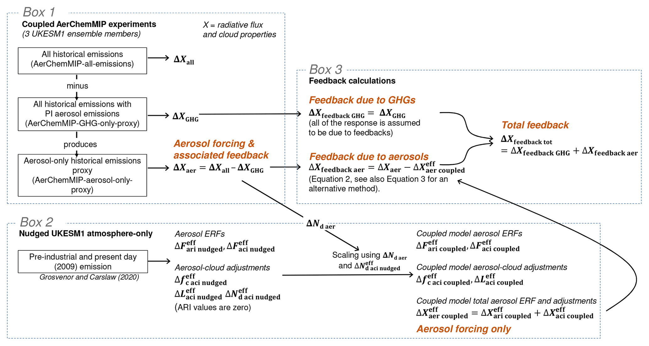
Figure 1Schematic showing how various quantities are calculated. Some of the quantities are not introduced until later in the paper. The same methodology also applies to the DAMIP (HadGEM-based) results except that GHG-only and aerosol-only proxies are not required (Box 1) since there are dedicated experiments with GHG-only and aerosol-only emissions.
2.2.3 The UKESM1 atmosphere-only run
We also examine data from the atmosphere-only UKESM1 runs performed as part of CMIP6, which have the same historical forcings as in the coupled CMIP6 runs but with sea-surface temperatures (SSTs) and sea-ice concentrations prescribed from observations. Examination of these simulations helps to quantify how deviations of the coupled model SSTs and sea ice from the observed state affect clouds and short-wave fluxes. It also allows for a model assessment of the atmospheric components against observations when given the correct ocean conditions. There is currently only one atmosphere-only run available, which prevents examination of the effects of atmospheric variability via an ensemble; for example, despite SSTs being fixed the atmosphere can exhibit different modes of variability that may not match the actual modes that occurred in reality, and so some differences between the atmosphere-only run and reality might be expected.
2.3 Surface albedo calculation and sea-ice screening
The surface albedo (Asurf) is required for the offline radiative calculations described in Sect. 3.2 and for the screening of high-sea-ice regions. It is calculated using the monthly mean upwelling and downwelling clear-sky SW surface fluxes ( and , respectively):
Grid boxes within the NA region were excluded where substantial sea ice was formed in any of the simulations such that the same grid boxes were excluded for all runs; the criteria for exclusion was the annual-mean surface albedo exceeding 20 % at some point during the historical time series.
2.4 Uncertainties in trends
Temporal trends are calculated using a linear least squares method, and the errors in the trends are calculated following Santer et al. (2000), where an effective sample size is used that takes into account temporal autocorrelation using the lag-1 autocorrelation coefficient.
2.5 MODIS cloud droplet number concentration observations
We use cloud droplet concentration (Nd) as an indicator of aerosol-driven changes in clouds, because it more directly represents the first step in the chain of processes by which aerosols affect clouds. Nd gives some indication of the number of cloud condensation nuclei (CCN; a subset of the whole aerosol population) that were available to produce clouds but is also affected by other factors such as updraught speed, droplet collision coalescence, droplet scavenging by rain, cloud evaporation, etc.
We evaluate model Nd and its trends against MODIS Nd observations. We use a 1 × 1∘ resolution data set calculated from 1 km MODIS retrievals of cloud optical depth (τc) and effective radius (re). Two-dimensional fields of Nd are derived by the retrieval since it is assumed that Nd is constant throughout the depth of the cloud, which has been shown to be a good approximation by aircraft observations of stratocumulus (Painemal and Zuidema, 2011). Details of the retrieval and dataset are given in Grosvenor and Carslaw (2020). For the model, two-dimensional Nd fields were obtained from the monthly 3D Nd fields by calculating a weighted vertical mean Nd, with the liquid water mixing ratio (qL) on each level used for the weights. This ensures that the levels with the most qL contribute most to the average Nd, which is similar to what is assumed in the MODIS retrieval since most of the re signal comes from near cloud top where qL is usually the largest, and the Nd calculation is a strong function of re. It also reduces the weight of contributions from very thin clouds that would not be detected by MODIS. Only datapoints for which the mean cloud top height is below 3.2 km were included for the satellite Nd calculation in order to help exclude satellite retrieval errors for deeper clouds (see Grosvenor et al., 2018).
2.6 Variables considered and assumptions for changes in short-wave flux
We attribute trends in FSW↑ to changes in liquid clouds, clear-sky FSW↑ and surface albedo. Changes in clear-sky FSW↑ () will include the effects of changes in aerosol in cloud-free air, changes in the surface albedo (Asurf) and changes in trace gas concentrations. However, we do not attempt to separate these effects here. For changes in the all-sky (i.e. combined cloudy and clear regions) albedo, we consider the effect of changes in the three main variables that affect it, namely cloud fraction (fc), cloud droplet number concentration (Nd) and in-cloud liquid water path (L), along with FSW↑ from the clear-sky regions above clouds and also Asurf in cloudy-sky conditions. However, changes in the latter were found to have negligible impact for the region considered. L is the LWP from the cloudy regions only. For fc, we use the total cloud fraction since liquid-only cloud fractions aggregated over all heights (i.e. accounting for overlap assumptions) were not available. Occasionally, the all-sky liquid water path (Lall-sky) is also considered (i.e. including both the cloudy and clear-sky portions of model grid boxes or observed regions). To calculate L from the Lall-sky values provided by the models, we assume that (e.g. as also in Seethala and Horváth, 2010); we use monthly values for this calculation.
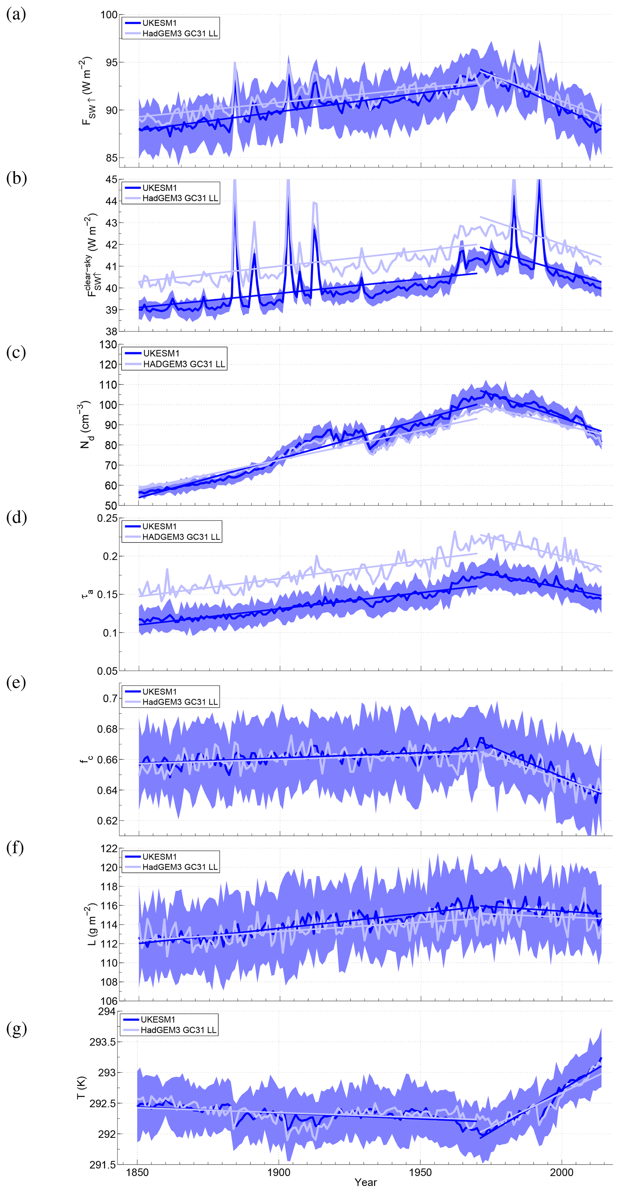
Figure 2Time series of annual mean values of various quantities from the UKESM1 model spatially averaged over the North Atlantic region (18–60∘ N, 0–75∘ W; ocean-only grid points with sea-ice regions excluded; see text for details). The blue shading denotes ± 2 times the standard deviation across the ensemble for UKESM1 only. (a) the all-sky upwelling SW flux at TOA (FSW↑); (b) the all-sky upwelling SW flux at TOA (); (c) The vertically averaged (weighted by liquid water content) cloud droplet concentration (Nd); (d) the aerosol+dust optical depth at 550 nm (τa); (e) Total cloud fraction (fc); (f) the in-cloud LWP (L); (g) The surface temperature (T).
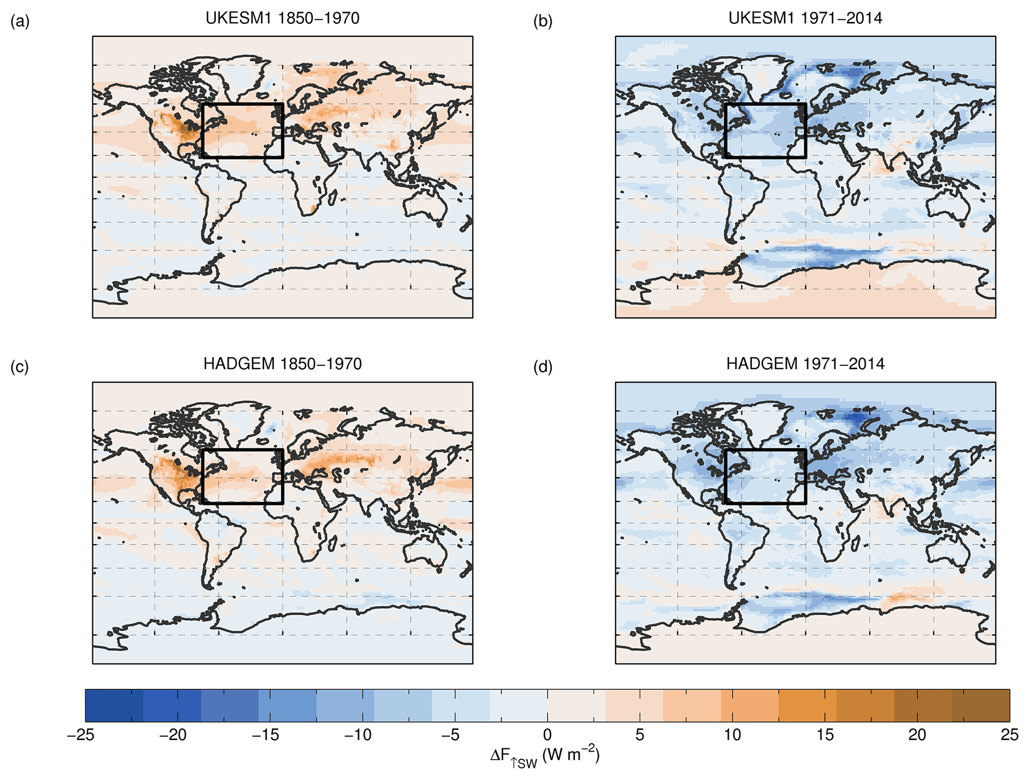
Figure 3Maps of the change in FSW↑ over the 1850–1970 (a, c) and 1971–2014 (b, d) periods for the ensemble means of the UKESM1 (a, b) and HadGEM (c, d) models. The region used for the time series analysis is shown by a black box; note that land regions and regions with substantial sea ice within the box were excluded (see text for details).
2.7 Calculation of aerosol radiative forcing
The effective radiative forcings (ERFs) due to aerosol–cloud interactions () and aerosol–radiation interactions () are considered. The total aerosol ERF () is the sum of the two. In the coupled climate runs, SSTs vary over time, and so ERFs cannot be directly calculated from the change in FSW↑ in aerosol-only emissions runs. Instead, the ERFs for the coupled climate runs (see Sect. 3.5) were estimated by scaling and from nudged simulations based on the ratio of the change in Nd over time in the coupled models to the change in Nd in the nudged runs (see Box 2 of Fig 1; Appendix C gives more details of the calculations). The nudged model runs consist of a pair of atmosphere-only nudged UKESM1 simulations with prescribed time-varying SSTs, as presented in Grosvenor and Carslaw (2020); one simulation used preindustrial (PI) aerosol emissions and the other present-day (PD) emissions from 2009. The nudging (using 2009 reanalysis) was applied only to the winds above the boundary layer and kept the large-scale meteorology approximately the same in both simulations whilst allowing local boundary layer and associated clouds to respond to the different aerosol loadings.
3.1 North Atlantic time series for UKESM1
Figure 2 shows UKESM1 and HadGEM time series averaged over a region of the North Atlantic (defined by the black box in Fig. 3 for ocean grid boxes with no substantial sea ice; see Sect. 2.3). The ensemble mean FSW↑ shows two long-term trends. The first is a positive trend between 1850 and approximately 1970; we denote this time period as pre-1970. The second is a negative trend from 1971 to the end of the simulation in 2014, denoted post-1970. FSW↑ values in 2014 and 1850 are similar despite the atmosphere not being free from anthropogenic influence at this time. The reasons for the similarity are discussed later.
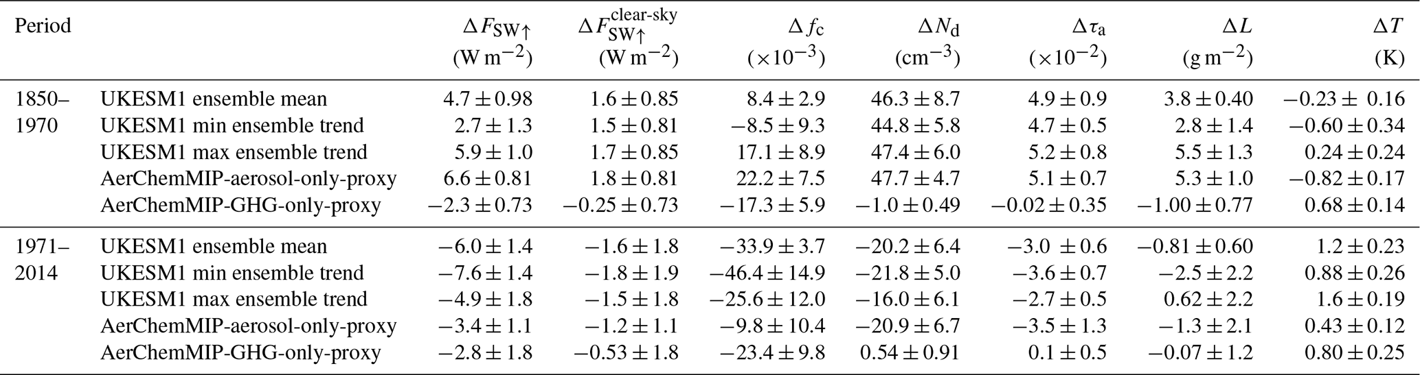
For each variable, trends have been fitted to the ensemble mean time series for the two periods and then multiplied by the duration of the time periods to give the total change in quantity x (denoted Δx). These values and the associated uncertainties in the fitted trends are given in Table 1. For the pre-1970 period for UKESM1, ΔFSW↑ was 4.7 ± 0.98 W m−2, and over the post-1970 period it was W m−2; hence, the magnitude of the change in FSW↑ is slightly larger for the second period. Short periods of enhanced FSW↑ are evident, which reach close to or extend beyond the 2σ variation of the ensemble. These are due to volcanic eruptions. One example occurs in 1991 and is due to the Mount Pinatubo eruption.
The maps of ΔFSW↑ in Fig. 3 show that the NA is one of the main oceanic regions that shows large changes in FSW↑ over the chosen time periods, which justifies the choice of this region as the focus of this paper. The other oceanic regions that show large changes are the Barents Sea (north of Scandinavia), the Southern Ocean and the northern Pacific. The Barents Sea and Southern Ocean changes in FSW↑ are likely to be related to sea-ice changes. The North American and western European continental regions also show large changes that are often larger than those over the ocean regions. For the pre-1970 period, the UKESM and HadGEM models are consistent in that larger changes in FSW↑ occur in the western North Atlantic region than in the east, suggesting a connection with pollution outflow from North America. This is also true for the post-1970 period for the HadGEM model, but for the UKESM model there is a stronger change in the eastern part of the North Atlantic, suggesting that different processes may be occurring compared to pre-1970 or potentially more natural variability in the spatial patterns.
We now discuss the potential drivers of changes in FSW↑. Cloud fraction shows a small increase over the pre-1970 period (Δfc = (8.4 ± 2.9) × 10−3), whereas over the post-1970 period there is a distinct decrease (Δfc = () × 10−3). The start of the negative trend in cloud fraction occurs at around the same time as the start of the negative trend in FSW↑ (1971). Nd shows a large increase over the pre-1970 period (ΔNd = 46.3 ± 8.7 cm−3) and, similarly to FSW↑ and fc, decreases (ΔNd = cm−3) after around 1971. Aerosol optical depth at 550 nm (τa, including dust) shows very similar trends to Nd although it is more variable. L increases over the pre-1970 period (ΔL = 3.8 ± 0.40 g m−2), indicating cloud thickening, but shows very little change over the post-1970 period (ΔL = 0.81± 0.60 g m−2). The reasons for the changes in the different cloud variables are discussed in Sect. 3.3.2.
The clear-sky top-of-atmosphere (TOA) radiative flux () also increases over the pre-1970 period ( = 1.6 ± 0.85 W m−2) and decreases thereafter. over the post-1970 period ( 1.8 W m−2) is the same magnitude but of opposite sign to that over the pre-1970 period. There are also large spikes in due to volcanic eruptions which are not present in the cloud variables, suggesting that the effect of volcanoes on FSW↑ occurs mainly via clear-sky effects. Note that the clear-sky effects are likely to be negligible in the cloudy parts of the grid boxes; hence, the values would need to be multiplied by the clear-sky fraction () to give the clear-sky contribution to the overall ΔFSW↑.
On the whole the changes in variables and trends in the HadGEM model are very similar to those for UKESM1 although with slightly smaller magnitude changes in FSW↑, Nd and L and larger magnitude changes in τa (see Table A1 and Appendix A for details on the HadGEM results). In addition, there is a notable difference in the magnitude of with HadGEM being around 1 W m−2 higher than UKESM1, which is consistent with the higher τa values. The reasons for this are left to other work to explore. Due to similarity of the two models, we mostly focus on the UKESM1 model for this paper and show results from HadGEM in Appendix A.
Table 1Changes in radiative fluxes and cloud properties (Δx values) over the 1850–1970 and 1971–2014 periods for the ensemble mean time series of the UKESM1 and AerChemMIP simulations. Also shown are the minimum and maximum Δx values across the UKESM1 16-member ensemble. The uncertainties are from the uncertainty in the fit lines used to calculate Δx.
3.2 Decomposing the FSW↑ trends in UKESM1 into contributions from individual variables
The above results show that the increase in FSW↑ over the pre-1970 period is likely to be caused by a combination of increases in Nd, L and since there is little change in fc. In contrast, for the post-1970 period the FSW↑ decrease is likely to be caused by decreases in fc, Nd and since L is fairly constant. To quantify the relative contributions of the changes in cloud properties to the changes in FSW↑, we first recreate the FSW↑ flux time series using offline radiative flux calculations with monthly ensemble mean fc, Nd, L, , downwelling SW at TOA and Asurf as inputs following the technique described in Grosvenor et al. (2017) and Grosvenor and Carslaw (2020) for TOA fluxes. The approach used here differs slightly to those studies due to the inclusion here of from the model for the clear-sky regions rather than assuming a constant transmissivity. Multiple scattering between the surface and cloud is also included here following Seinfeld and Pandis (2006). The offline radiative flux calculations can then be used to quantify the individual contributions from the changes in the different cloud properties.
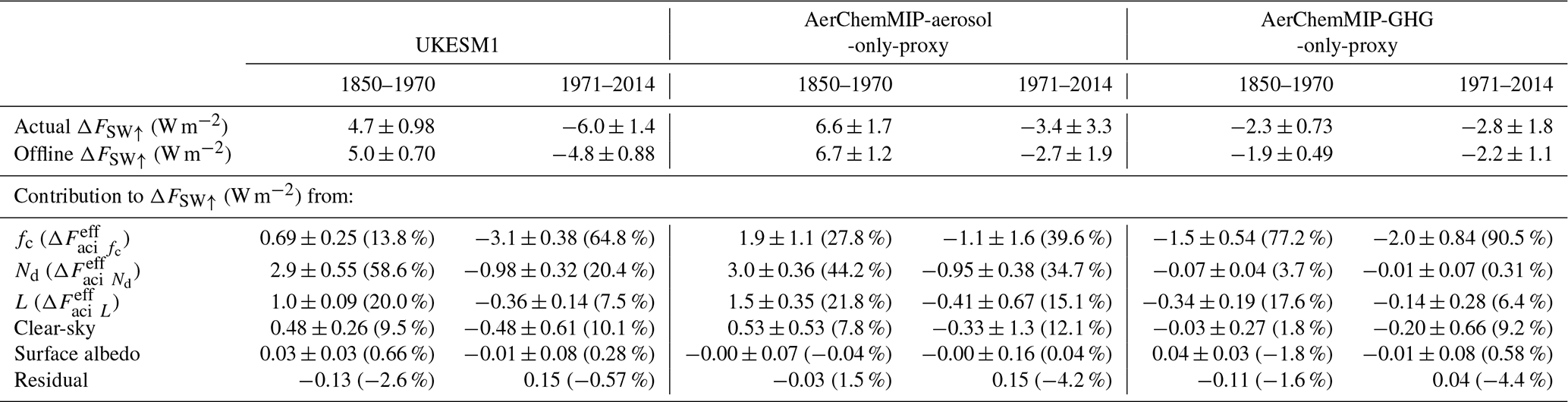
Figure 4a compares the reconstructed FSW↑ flux time series with the time series from the model (i.e. that calculated online by the UKESM1 at each radiation time step of the model, as previously shown in Fig. 2). The inter-annual variability of the calculated fluxes match those from the model output very well. The ΔFSW↑ values from the reconstructed time series are similar to the actual model values during the pre-1970 period and the post-1970 period (see Table 2), although with a 6 % overestimate for the pre-1970 period (ΔFSW↑ = 5.0 vs. 4.7 W m−2 for the estimated vs. actual values, respectively) and a 20 % underestimate in the absolute magnitude of ΔFSW↑ for the post-1970 period (ΔFSW↑ = −4.8 vs.−6.0 W m−2). Despite these discrepancies, the appearance of a positive trend in the pre-1970 period and a negative trend in the post-1970 period, along with trends that are close to those from the full model gives confidence that the reconstructed radiative fluxes are sufficient for estimating the contributions from the individual cloud properties to ΔFSW↑.
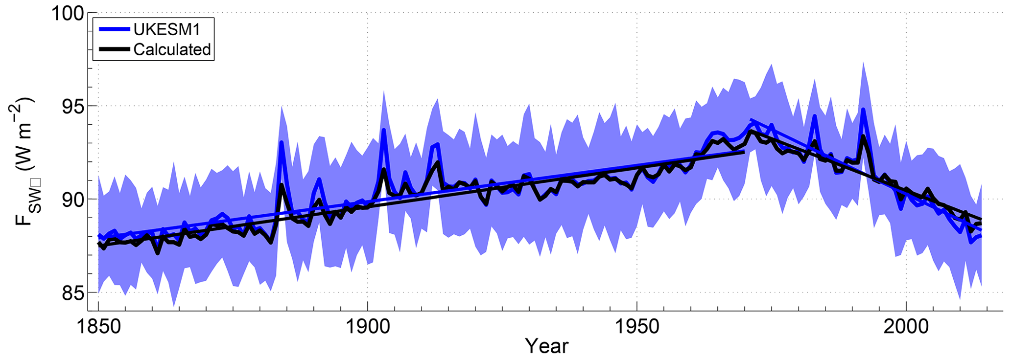
Figure 4Time series of annual mean FSW↑ as calculated using the offline radiative transfer model (labelled “Calculated”) and that directly from the model output for the UKESM1. The blue shading denotes ± 2 times the standard deviation across the ensemble for the model output data. The region for area averaging is the same as for Fig. 2.
The individual contributions to ΔFSW↑ were estimated by recalculating the FSW↑ fluxes and the linear trends in ΔFSW↑ for the two periods while holding the other cloud properties fixed at the time-mean value for each time period.
For the pre-1970 period, all variables cause an increase in FSW↑ trend. The trend in Nd contributes most to ΔFSW↑ (Fig. 5 and Table 2) with 58.6 % of the total, followed by L (20.0 %), then fc (13.8 %) and (9.5 %), with a −2.6 % residual. For the post-1970 period, the largest influence is the reduction in fc which explains 64.8 % of ΔFSW↑. However, the decrease in Nd also has some influence (20.4 %). and L decrease slightly over this period but have minimal influence on the FSW↑ change (10.1 % and 7.5 %), respectively, and with large uncertainties. There is a small residual of −0.57 %.
These results show that the long-term changes in FSW↑ over the pre-1970 period are dominated by cloud brightening via the Twomey effect (i.e. an increase in Nd with other cloud properties held constant). The increase in the macrophysical cloud properties, L and fc, which account for a combined 33.8 % of ΔFSW↑, could indicate some cloud adjustments in response to changes in Nd but could also be influenced by non-aerosol factors such as changes in SST, air temperature, or atmospheric and oceanic circulation. These effects will be discussed in the next section. For the post-1970 period, the Twomey effect (−0.98 W m−2) is considerably smaller in magnitude than for the pre-1970 period (2.9 W m−2), because ΔNd is only cm−3 in the post-1970 period compared to 46.3 ± 8.7 cm−3 in the pre-1970 period. Another factor is that cloud albedo, and hence FSW↑, is more sensitive to changes in Nd when Nd is lower (Carslaw et al., 2013), so the reduction in Nd between its peak in 1971 and 2014 will have had less effect on FSW↑ compared to the same ΔNd in the pre-industrial-like conditions of 1850; ΔFSW↑ for the post-1970 period is 34 % of the pre-1970 value, whereas the post-1970 ΔNd is 44 % of the pre-1970 value. The much larger change in fc during the post-1970 period compared to the pre-1970 period suggests that the reduction in fc is unlikely to be dominated by cloud adjustments to aerosol given that the change in Nd is much smaller over the post-1970 period than over the pre-1970 period. There are several factors that could influence the macrophysical cloud changes during the two periods, and we now attempt to quantify the influence of the individual drivers.
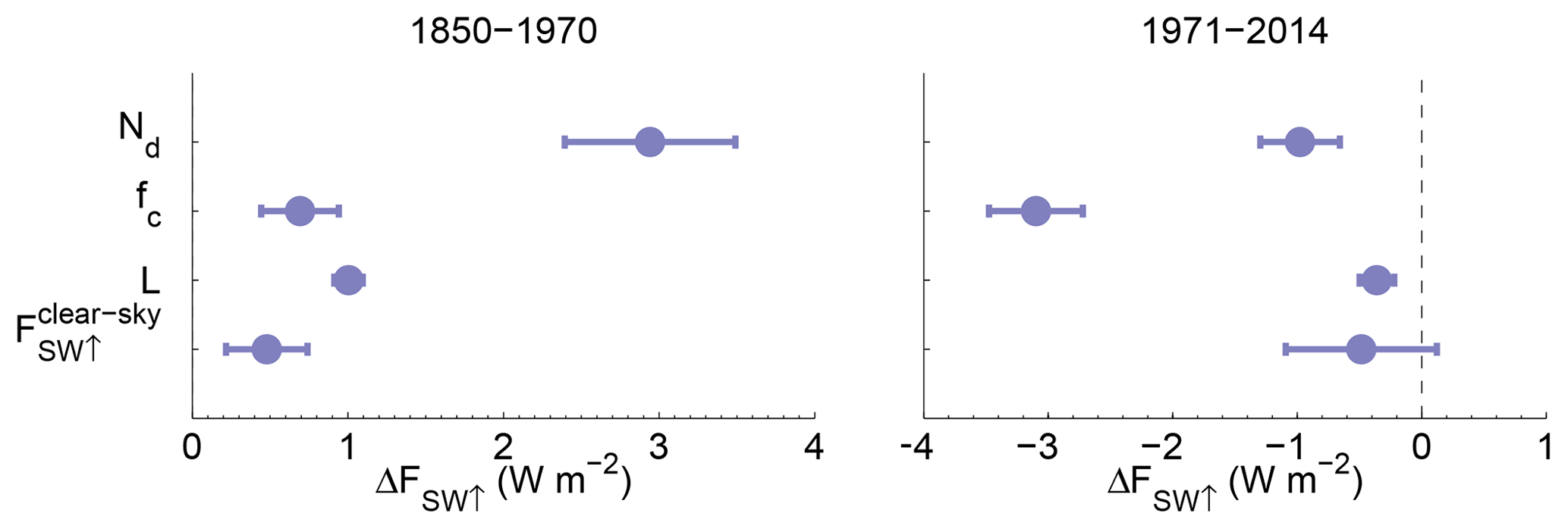
Figure 5Estimated contributions to the change in FSW↑ (ΔFSW↑) between 1870 and 1970 (the pre-1970 period) and between 1971 and 2014 (the post-1970 period) due to changes in Nd, fc, L and calculated using an offline radiative transfer algorithm by allowing only one variable at a time to vary. All results are for the UKESM1 model.
Table 2ΔFSW↑ values for the two periods. Shown are the actual values from the model output (online radiative calculations), the reconstructed values (using offline radiative calculations with all variables changing over time) and the estimated contributions from changes in fc, Nd, L, clear-sky FSW↑ () and surface albedo. NB: the surface albedo contribution here only includes that from cloudy conditions; the effect of surface albedo in clear skies is included in . The contributions are also quoted as percentages of the full offline values (offline radiative calculations with all variables changing over time). Residuals from the full offline values are also listed.
3.3 Quantifying the effects of individual emission types on FSW↑ and cloud variable changes
So far we have attributed the changes in ΔFSW↑ to changes in cloud and aerosol properties. We now attempt to attribute the changes in radiative fluxes and the associated cloud variables to changes in emissions (see Sect. 2.2.2) in UKESM1, based on the AerChemMIP experiments and in HadGEM (see Appendix A) based on the DAMIP experiments. We do this for several variables (FSW↑, , Nd, τa, fc, L and surface temperature) by fitting trends to the AerChemMIP and DAMIP time series for the pre-1970 period and the post-1970 periods and calculating the change in the trend lines as a Δx value as described in Sect. 3.1. The values are listed in Table 1.
3.3.1 Effect of emissions on FSW↑ and
Figure 6 shows the time series of FSW↑ and the cloud variables expressed as an anomaly relative to the 1850–1859 mean for the AerChemMIP aerosol-only and greenhouse gas-only proxies (see Sect. 2.2.2). Anthropogenic aerosol emissions (AerChemMIP-aerosol-only-proxy) generally cause an increase in FSW↑, whereas greenhouse gas emissions (AerChemMIP-GHG-only-proxy) cause a decrease. When all emissions are applied (AerChemMIP-all-emissions), the effects of aerosols and greenhouse gases act in opposite directions, resulting in a smaller-magnitude change in FSW↑ than would occur with only one of the emission types. For the majority of the time series, changes in aerosols have the most influence; therefore, there is an overall increase in FSW↑ over most of the time series. However, by the end of the time series, FSW↑ is similar to the value at the start.
Figure 7 and Table 1 summarize the contributions of each emission type to ΔFSW↑ in UKESM1. For the pre-1970 period, the ΔFSW↑ estimated to be due to aerosol emissions is 6.6 ± 1.7 W m−2 (see Table 1), which is much larger in magnitude than the reduction in FSW↑ caused by greenhouse gas emissions (−2.3 ± 0.73 W m−2). However, the reduction due to greenhouse gases is still important and shows that in the models with all emissions applied the effect of SW aerosol forcing is offset by around 35 % by opposing greenhouse gas effects. For the post-1970 period, there is less contribution from aerosol emissions (−3.4 ± 3.3 W m−2), which is consistent with the smaller-magnitude change in Nd due to aerosol emission reductions (−20.9 ± 6.7 vs. 47.7 ± 4.7 cm−3 for the pre-1970 period). There is a similarly sized negative contribution from greenhouse gas emissions (−2.8 ± 1.8 W m−2).
For , only the aerosol emissions drive meaningful trends, suggesting that greenhouse gas-driven changes in clear-sky SW are negligible (e.g. those caused by changes in water vapour or gaseous absorption).
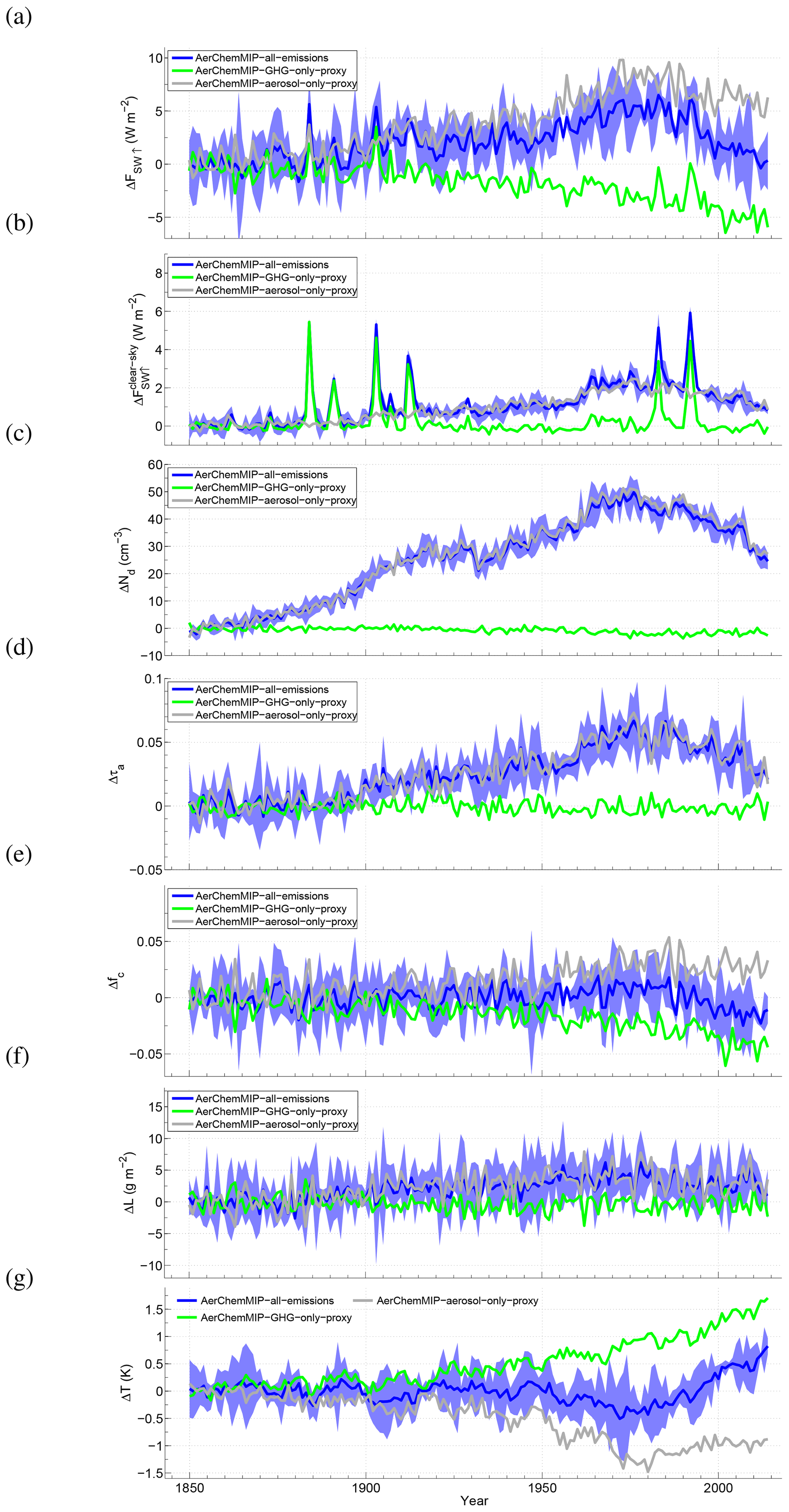
Figure 6Same as for Fig. 2 except for the various single-emission AerChemMIP proxy simulations and that values are expressed as a perturbation from the average over the first 10 years of simulation for each line. Lines are shown for AerChemMIP-all-emissions, AerChemMIP-aerosol-only-proxy and AerChemMIP-GHG-only-proxy.
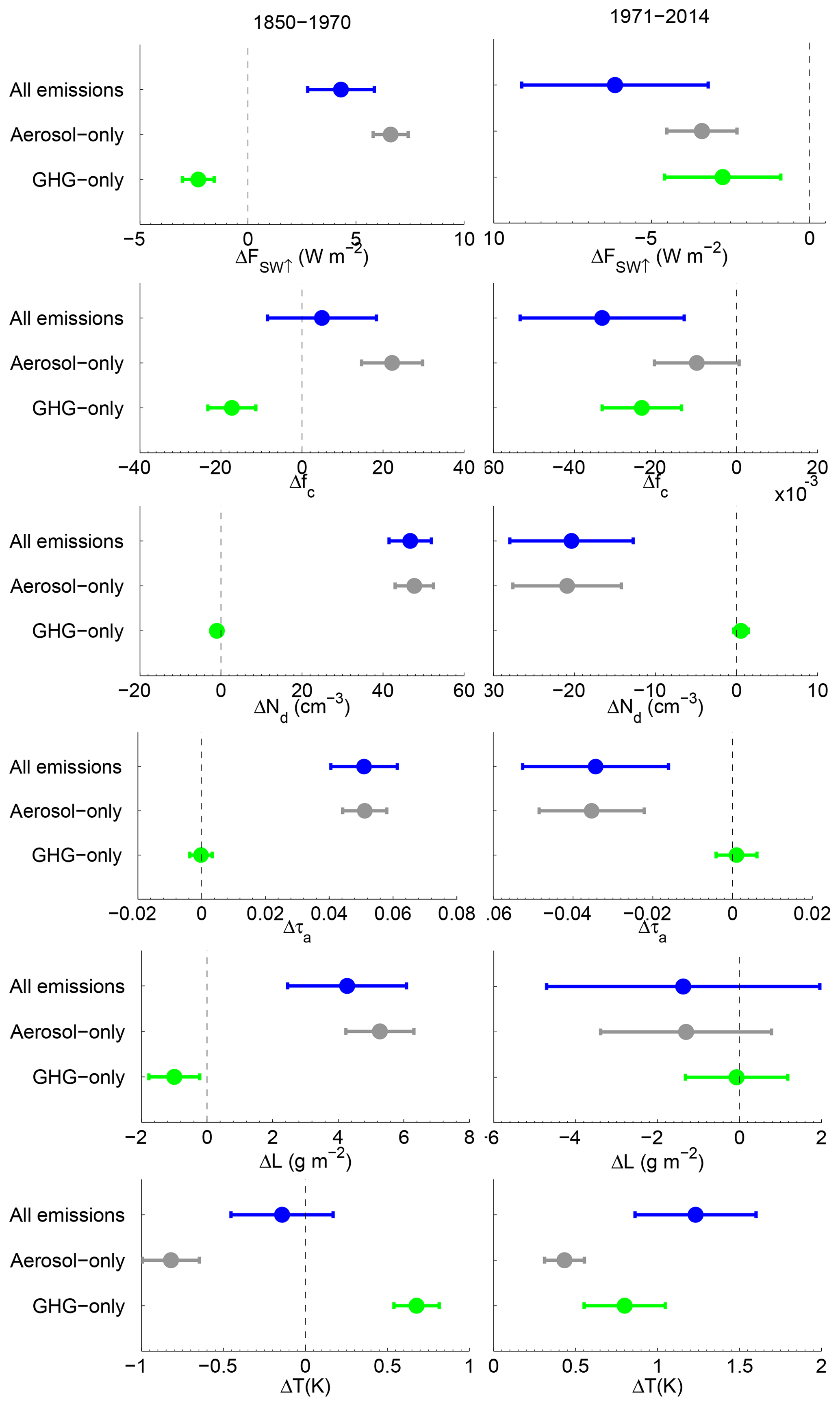
Figure 7Changes in various quantities for the 1850–1970 period (left column) and the 1971–2014 period (right column) for the AerChemMIP UKESM1 experiments. Results are shown for the AerChemMIP-GHG-only-proxy, AerChemMIP-aerosol-only-proxy and AerChemMIP-all-emissions experiments.
3.3.2 Effect of emissions on fc, Nd, L and τa
We next consider how the individual emission types affect the underlying cloud variables that were shown in the previous sections to drive the changes in FSW↑. Figure 7 shows the overall changes in fc, Nd and L for AerChemMIP-all-emissions, AerChemMIP-aerosol-only-proxy and AerChemMIP-GHG-only-proxy.
Figure 7 shows that the magnitude of the greenhouse gas-driven decrease in fc is slightly larger in the post-1970 period than in the pre-1970 period. Aerosols cause a positive Δfc in the pre-1970 period and a slightly negative Δfc in the post-1970 period. Figure 5 showed that in the pre-1970 period for the UKESM1 run there is little net contribution to ΔFSW↑ from changes in fc with changes in Nd dominating. The results for the UKESM all-emissions run in Figs. 6 and 7 show that this is due to a fairly small net change in fc during this period for UKESM1 relative to the post-1970 period. However, the AerChemMIP experiments suggest that this small change in fc is the result of opposing large changes due to the aerosol and greenhouse gas emissions.
Changes in Nd (and τa) are dominated by the aerosol emissions during both periods with virtually no contribution from greenhouse gases. This indicates that the substantial changes to climate from greenhouse gases have no effect on Nd or aerosols in this model. It is conceivable that changes in cloud location, cloud coverage, updraught speeds or precipitation in response to greenhouse gases could affect Nd, but this appears not to be the case for this model.
The dominant driver of ΔL (Figs. 6 and 7) during the pre-1970 period is aerosol emissions (AerChemMIP-aerosol-only-proxy), and there is no significant change in L due to greenhouse gas emissions. During the post-1970 period, contributions to ΔL from greenhouse gases are near zero, and there is a small negative aerosol contribution. However, the uncertainties for this period are larger than the values indicating that they are likely spurious.
3.3.3 Effect of emissions on surface temperature
During the pre-1970 period, the warming from greenhouse gases (0.68 ± 0.14 K) and the cooling from aerosols (−0.82 ± 0.17 K) roughly cancel out to give a net change in temperature that is nearly zero (−0.14 ± 0.19 K). During the post-1970 period, greenhouse gases produce a warming of 0.80 ± 0.25 K that is similar to that for the pre-1970 period, although it occurs within a shorter time frame (i.e. the trend is larger). Aerosol emissions declined during the post-1970 period; hence, there is also a warming effect from aerosols of 0.43 ± 0.12 K, which is around half the greenhouse gas warming.
3.4 Decomposing the FSW↑ trends in the single-emissions experiments into contributions from individual cloud and aerosol variables
In this section we perform the same analysis as in Sect. 3.2 to quantify how much the individual changes in aerosol and cloud properties contribute to ΔFSW↑ except for the single-emissions experiments (aerosol-only and GHG-only). It is clear from the DAMIP experiment results in Figs. A1 and A3 and Table A1 (see Appendix A) that the DAMIP natural aerosol forcing, which comes mostly from volcanic aerosols, has almost no influence on the FSW↑ trends; therefore, we do not consider natural aerosols further. However, there could be influences from natural aerosols that are not captured by the DAMIP natural emissions such as feedbacks between sea-spray CCN and temperature. Some of these will be represented in the experiments used here such as the effects on sea spray from changes in wind speed as a result of temperature change. Our results (Table 1 and Fig. 6d) show that there is little change in Nd in the AerChemMIP-GHG-only-proxy experiment (1.0 ± 0.49 cm−3 for the pre-1970 period and 0.54 ± 0.91 cm−3 for the post-1970 period) in which large changes in temperature occur, which suggests little influence of climate feedbacks on CCN. Our results are likely to exclude the impact of changes in sea spray due to changes in sea-ice coverage since we deliberately excluded sea-ice-covered regions. Therefore we calculated the changes in Nd for only the sea-ice regions and found values of 0.57±0.47 and −0.84 ± 0.74 cm−3 for the pre- and post-1970 periods, respectively, suggesting that the effect is small for this model.
3.4.1 Aerosol-only emissions
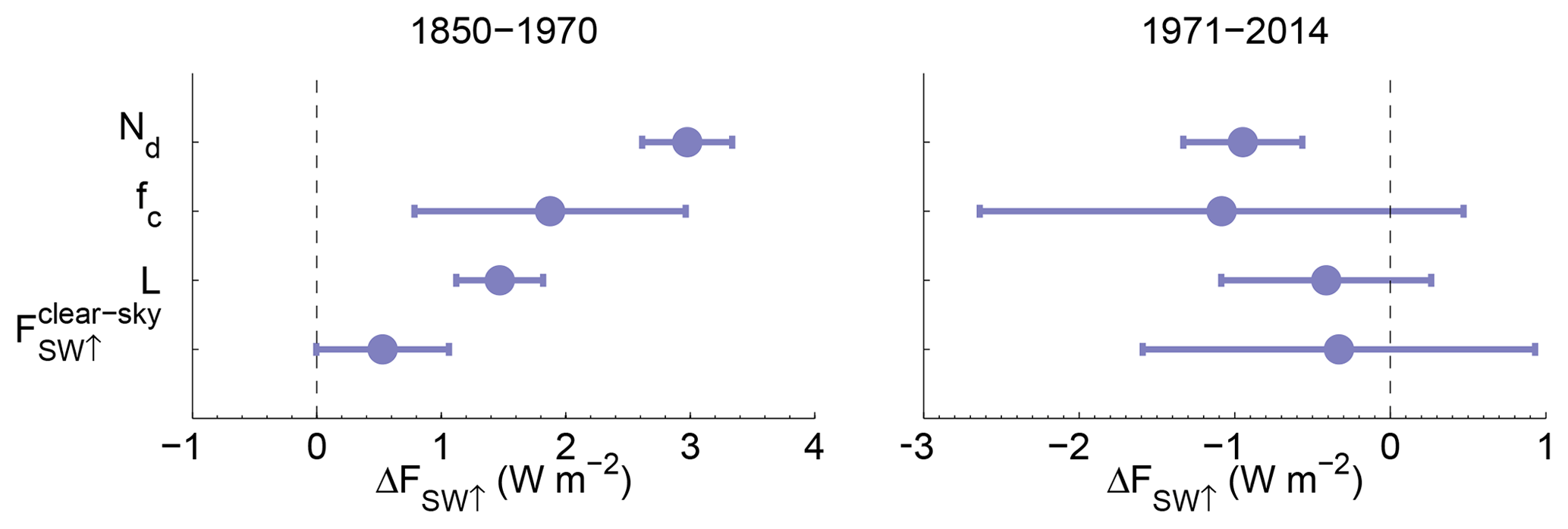
Figure 8 shows the contributions to ΔFSW↑ from the changes in the different aerosol and cloud variables for the AerChemMIP-aerosol-only-proxy run calculated, as in Sect. 3.2, using offline radiative calculations. Percentages are quoted relative to the offline-estimated total ΔFSW↑ for the AerChemMIP-aerosol-only-proxy (6.7 ± 1.2 W m−2) rather than the actual ΔFSW↑ (6.6 ± 1.7 W m−2). ΔNd provides the largest contribution during the pre-1970 period (3.0 ± 0.36 W m−2 or 44.2 % of the total). The Δfc contribution is significantly smaller (1.9 ± 1.1 W m−2 or 27.8 %) with the ΔL contribution (21.8 %) being slightly smaller still. The contribution is small and uncertain at 0.53 ± 0.53 W m−2 or 7.8 %.
The small contribution in the pre-1970 period indicates that the ARI forcing is quite small, which is consistent with Grosvenor and Carslaw (2020). The large ΔNd contribution shows that the Twomey ACI effect is very important in driving the ΔFSW↑ from aerosols. However, the contributions from changes in the cloud macrophysical properties (fc and L) are slightly more important than the Twomey ACI effect when considered together, comprising 49.1 % of the ΔFSW↑ change compared to 44.2 % from the cloud microphysical response (i.e. due to Nd changes). However, in Sect. 3.5.2 we show that some of the changes in fc and potentially in L are due to cloud feedbacks that are likely to have been induced by changes in temperature, and hence they do not solely represent forcing via cloud adjustments.
For the post-1970 period, the contribution to the total ΔFSW↑ (−2.7 ± 1.9 W m−2) from changes in Nd is −0.95 ± 0.38 W m−2. The contribution from changes in fc is also negative and of a similar magnitude but highly uncertain (−1.1 ± 1.6 W m−2). The L and contributions (−0.41 ± 0.67 W m−2 and −0.33 ± 1.3 W m−2, respectively) are smaller and also very uncertain. Changes in the macrophysical cloud properties (fc and L; 54.1 %) therefore dominate over those of the microphysical variables (Nd; 34.7 %), although the macrophysical contributions are highly uncertain.
3.4.2 Greenhouse gas-only emissions
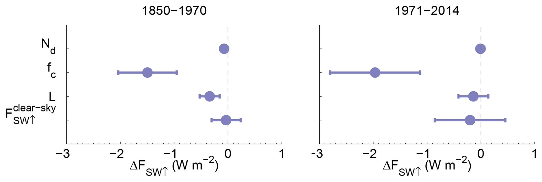
The effects of greenhouse gases on ΔFSW↑ are almost entirely driven by changes in fc for both the pre-1970 period and the post-1970 period (Fig. 9) with a larger magnitude of contribution for the post-1970 period (−2.0 ± 0.84 vs. −1.5 ± 0.54 W m−2 in the pre-1970 period) despite the post-1970 period being a shorter span of time. This is likely due to an enhanced rate of greenhouse gas emissions during the post-1970 period resulting in a more rapid temperature increase.
3.5 Aerosol forcing vs. cloud–climate feedbacks
Here we examine the relative roles of aerosol forcing and feedbacks resulting from climate change (temperature, atmospheric/ocean circulation changes, etc.) on the change in FSW↑ and the cloud variables.
Aerosol forcing is the change in FSW↑ caused by a change in aerosols without a change in climate (SSTs, water vapour, atmosphere and ocean circulation, etc.). This includes rapid cloud adjustments of fc and L which are potentially a major cause of changes in FSW↑.
For the greenhouse gas-only runs, we assume that the changes in FSW↑, fc and L are due to climate feedbacks with no effect of greenhouse gases on cloud or clear-sky adjustments. However, we acknowledge that such effects may be possible. For example, the results of Andrews and Forster (2008) showed a −0.18 W m−2 global change in FSW↑ from greenhouse gas adjustments (termed semi-direct forcing in that paper) for the HadGEM1 model in a doubling CO2 experiment. This would represent a small fraction (6.4 %) of the −2.8 W m−2 change from the AerChemMIP-GHG-only-proxy run for the post-1970 period (although the latter is for the North Atlantic region only) and is also likely to be an overestimate for our case since the change in CO2 for the post-1970 period is less than a doubling. Furthermore, Fig. 7.4 of the AR6 assessment (Forster et al., 2021) estimates the global CO2 adjustment effect to be around 5 % of the total ERF, although this is for the combined short-wave and long-wave values.
For the AerChemMIP-aerosol-only-proxy runs, changes in FSW↑, fc and L are split between aerosol forcing and climate feedback terms using two different methods. The first method estimates the feedback term as the change of the quantity (ΔXaer, where X represents either FSW↑, fc and L for the AerChemMIP-aerosol-only-proxy run) minus the change in X induced by the aerosol effective radiative forcing ():
See Box 3 in Fig. 1. Here, was calculated using the results from the nudged runs of Grosvenor and Carslaw (2020) (see Box 2 in Fig. 1, Sect. 2.7 and Appendix C).
The second method estimates the change in X due to climate feedbacks () in the AerChemMIP-aerosol-only-proxy run using the temperature change in that run (ΔTaer) based on the sensitivity of X to temperature in the AerChemMIP-GHG-only-proxy run:
where ΔXGHG and ΔTGHG are the changes in X and temperature, respectively, in the AerChemMIP-GHG-only-proxy run.
The climate feedback term could include several processes. For example, aerosol and greenhouse gas forcing can change global and local temperatures and sea ice which can then cause changes in atmospheric and oceanic circulation, and subsequent changes in the distribution of aerosols and clouds. There is evidence that warming can cause an expansion of the Hadley cell and a poleward shift of the storm tracks (Held and Hou, 1980; Lu et al., 2007; Seidel et al., 2008) that can reduce mid-latitude cloudiness (Norris et al., 2016). Cooling would have the opposite effect, leading to increases in FSW↑ in the North Atlantic region. It has also been suggested that aerosols may have a local influence on the Atlantic Meridional Overturning Circulation (AMOC) that is more direct than the effect of aerosols on large-scale temperatures (Yu and Pritchard, 2019; Robson et al., 2022). Menary et al. (2020) show that the AMOC speeds up in the DAMIP-Hist-Aer run as a result of aerosol emissions, and it is feasible that changes in the AMOC could also lead to changes in cloud cover or properties and hence changes in FSW↑.
3.5.1 Forcing vs. feedbacks for FSW↑
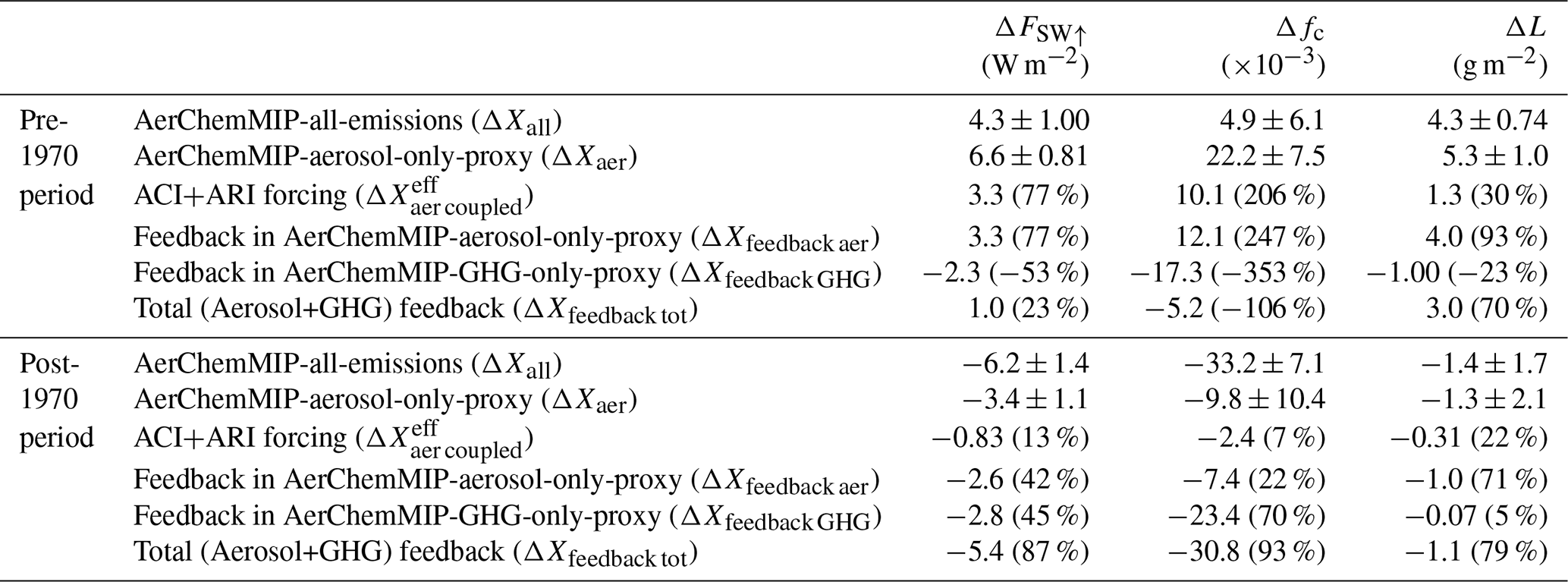
The balance between aerosol forcing and climate feedbacks is first examined for ΔFSW↑. Figure 10 shows that for both periods is much larger than for the AerChemMIP-aerosol-only-proxy run. For the pre-1970 period, the estimated aerosol ERF ( + ) of the AerChemMIP-aerosol-only-proxy run accounts for 77 % of the ΔFSW↑ of the all-emissions run (see Table 3). Climate responses in the AerChemMIP-aerosol-only-proxy run (labelled “Aerosol Feedback” in Fig. 10) also account for 77 % of the ΔFSW↑ of the all-emissions run, showing that the initial aerosol ERF and the subsequent climate feedbacks are equally important in causing changes in FSW↑ in the aerosol-only run. The ΔFSW↑ from the AerChemMIP-GHG-only-proxy run (assumed to be all due to climate feedback) was −53 % of ΔFSW↑ of the all-emissions run which brings the total of the aerosol forcing, aerosol-driven cloud–climate feedback and greenhouse gas-driven cloud–climate feedback terms to 100 %. Figures 6 and 7 show that during the pre-1970 period aerosols caused a cooling of around 0.85 K in AerChemMIP-aerosol-only-proxy. This is likely to have caused a climate response that affected FSW↑, for example, via an increase in cloud fraction due to mid-latitude cloud feedbacks. The value (Eq. 3) is another estimate of this cloud–climate feedback using the above temperature change for aerosol-only emissions and is shown in Fig. 10 as the “Aerosol Feedback from ΔT” datapoint. It shows good agreement with the “Aerosol Feedback” value, suggesting that the local temperature change is a good indicator of the feedback contribution.
If ΔFSW↑ from the greenhouse gas-driven cloud–climate feedback (from the AerChemMIP-GHG-only-proxy run) is added to the aerosol-driven cloud–climate feedback value (“Aerosol Feedback”), then we obtain an estimate of the overall change in FSW↑ due to feedbacks from both types of emissions. For the pre-1970 period, this overall feedback effect on FSW↑, termed “Total (Aerosol Feedback + GHG) Feedback”, is considerably lower in magnitude than the aerosol forcing term and accounts for 23 % of ΔFSW↑ from the all-emissions run (cf. 77 % for aerosol forcing). This indicates that in the all emissions run, which is assumed to be the run most similar to the real world, the aerosol forcing has a larger influence on FSW↑ than climate feedbacks during the pre-1970 period. This dominance of aerosol forcing is mainly due to the cancellation of the warming effect of greenhouse gases and the cooling effect of aerosols (Figs. 6 and 7).
For the post-1970 period, the aerosol ERF is in the opposite direction and is smaller in magnitude than for pre-1970 as expected from the smaller-magnitude change in Nd. The estimated change in FSW↑ due to aerosol-driven cloud feedbacks is now negative in contrast to the pre-1970 period, which is consistent with the increase in temperature caused by aerosols during the post-1970 period (Figs. 6 and 7). The sign of ΔFSW↑ estimated from the temperature change (“Aerosol Feedback from ΔT”; Eq. 3) is in agreement with the ΔFSW↑ due to aerosol-driven cloud feedbacks, although it is a little lower in magnitude. For the post-1970 period, the total change in FSW↑ due to feedbacks associated with aerosols and greenhouse gases is considerably larger in magnitude (87 % of the all-emissions run value) than the overall aerosol forcing (13 %). This implies that observations of changes in FSW↑ over the post-1970 period cannot be used directly to evaluate aerosol forcing in models without taking account of feedbacks.
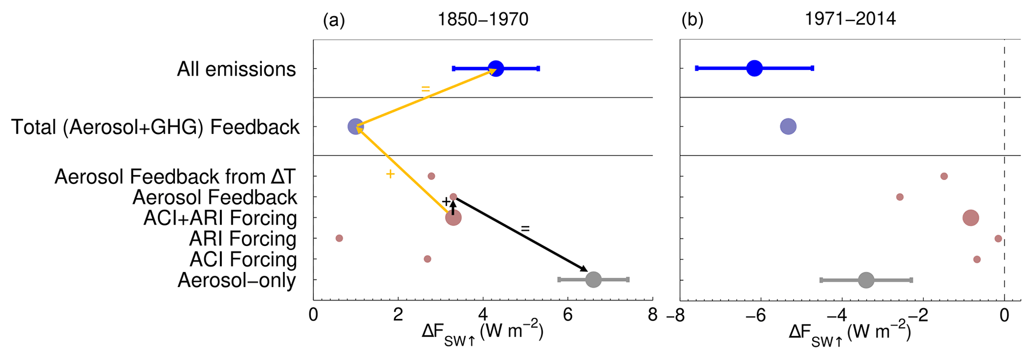
Figure 10The relative roles of aerosol forcing and climate feedbacks in explaining ΔFSW↑ between 1870 and 1970 (a) and between 1971 and 2014 (b) for the AerChemMIP UKESM1 runs. “Aerosol-only” is the change in the AerChemMIP-aerosol-only-proxy runs as in Fig. 7 (ΔFSW↑ aer). “ACI” and “ARI” are the aerosol effective radiative forcings ( and ). “Aerosol Feedback” is the climate feedback term for the AerChemMIP UKESM1 runs (ΔFSW↑ feedback aer) calculated using Eq. (2), and “Aerosol Feedback from ΔT” () is that calculated using Eq. (3). “Total (Aerosol + GHG) Feedback” is the estimated total climate feedback in the all-emissions run (ΔFSW↑ feedback tot) calculated by summing ΔFSW↑ from the AerChemMIP-GHG-only-proxy run (ΔFSW↑ feedback GHG) and ΔFSW↑ feedback aer. Also shown is ΔFSW↑ for the all-emissions UKESM1 AerChemMIP runs (AerChemMIP-all-emissions). Arrows in panel a are drawn to indicate values that add together to give other values on the plot (see Eq. 2 and Appendix D). These also apply to panel b and to all panels for Figs. 11 and 12 but are omitted for clarity. The black arrows also apply to the DAMIP experiments (Figs. A6, A7 and A8), but the orange ones do not. Arrows for have also been omitted.
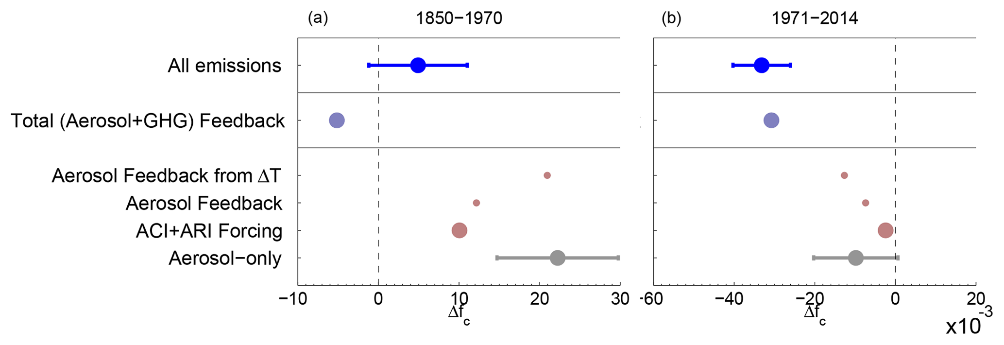
3.5.2 Forcing vs. feedbacks for fc, Nd and L
The changes in cloud variables from the AerChemMIP-aerosol-only-proxy run are further split into forcing and climate feedback components in a similar way to how the ΔFSW↑ term was split earlier, i.e. using the results from the nudged runs of Grosvenor and Carslaw (2020) (see Sect. 2.7 and Appendix C). Note that for fc and L it is not possible to split the forcing into ARI and ACI terms since in Grosvenor and Carslaw (2020) this could only be done for FSW↑.
For the pre-1970 period (Fig. 11), slightly more of Δfc (247 % of the Δfc of the all-emissions run) in AerChemMIP-aerosol-only-proxy comes from the climate feedback effect rather than the aerosol forcing (206 %). Likewise, most of the ΔL (Fig. 12) comes from the climate feedback (93 %) with 30 % coming from the aerosol forcing. Hence most of the contributions to ΔFSW↑ in AerChemMIP-aerosol-only-proxy from Δfc and ΔL seen in Fig. 8 are from the climate responses to the increase in aerosol rather than cloud adjustments.
For the post-1970 period, the aerosol-induced changes in fc and L are negative, which is consistent with the sign of the aerosol forcing. The predicted aerosol forcings are very small for both variables. The estimated climate feedback terms are larger in magnitude than the aerosol forcings; however, the uncertainties in the aerosol-induced changes are large, particularly for L.
Figure 7 showed that there was little change in L in the AerChemMIP-GHG-only-proxy run for either period. This is a little surprising since greenhouse gas forcing caused a large reduction in fc during both periods, presumably through climate response changes. Hence, given the estimated large response of L to climate responses in AerChemMIP-aerosol-only-proxy (Fig. 12), a fairly large climate response for L due to greenhouse gas forcing may have been expected. It is possible that the aerosol and greenhouse gas-induced climate responses are somewhat different and have different effects on clouds, although we also note that the L time series is particularly noisy (Fig. 6) such that the AerChemMIP-GHG-only-proxy error bar for L (Fig. 7) for the post-1970 period extends into negative values, and the error bar for AerChemMIP-aerosol-only-proxy in Fig. 12 is large enough to be consistent with a much smaller climate response or even a zero climate response with the aerosol forcing accounting for all of the change. However, the uncertainties for the pre-1970 period are much smaller, suggesting that the above arguments do not apply for that period. In that case the large increase in ΔL in response to aerosol-induced climate feedbacks during the pre-1970 period when uncertainties were lower might indicate that some of the ΔL during the post-1970 period was caused by a similar circulation change in reverse (due to the opposite sign of ΔT over the two periods). It is also possible that the magnitude of the aerosol forcing for L is underestimated, which would produce a smaller estimate for the magnitude of the climate feedback contribution for AerChemMIP-aerosol-only-proxy. Determining the reasons for the above surprising result is left to future work.
As discussed in Sect. 3.3, Figs. 6 and 7 show that there is no change in either Nd or over the two periods in the AerChemMIP-GHG-only-proxy run despite the large climate responses to greenhouse gas emissions. It is therefore likely that there was also no impact upon Nd or from the climate responses in the AerChemMIP-aerosol-only-proxy run and hence that the changes in these variables are almost entirely driven by the aerosol changes. This suggests that almost all of the ΔFSW↑ that was apportioned to climate responses in the AerChemMIP-aerosol-only-proxy run (Fig. 10) was due to the associated changes in fc and L.
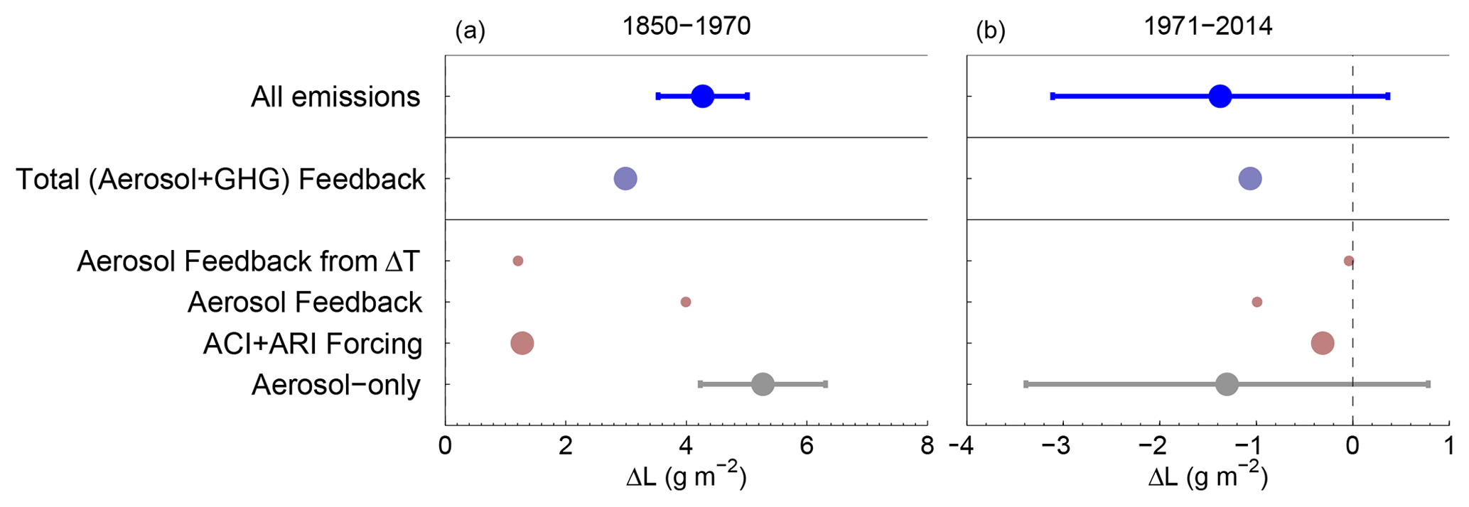
Figure 12Same as for Fig. 10 except for L and that the aerosol forcing term is not further split into ACI and ARI contributions.
Table 3Contributions to changes in FSW↑, fc and L from various processes as in Figs. 10, 11 and 12 along with the addition of the changes from the AerChemMIP-GHG-only-proxy run (assumed to be the climate feedback term for that run) for the UKESM1-based AerChemMIP experiments. The percentages in brackets are the contribution expressed as a percentage of the contribution of the AerChemMIP-all-emissions run.
We now compare the modelled time series with observations. Reliable observations are only available in the later parts of the time series. For FSW↑, we use the DEEP-C dataset (Allan et al., 2014b) that is available from 1985–2014; for Nd we use MODIS data from 2003–2012 (see Sect. 2.5 for details); for τa we use 2003–2012 Level-3 MODIS Aqua monthly mean data from the combined 550 nm Dark Target and Deep Blue product “Dark_Target_Deep_Blue_Optical_Depth_550_Combined” (Levy et al., 2013); for fc we use PATMOSx and ISCCP data from Norris et al. (2016) for 1983–2009; for Lall-sky we use the MAC-LWP (Multi-Sensor Advanced Climatology of Liquid Water Path) microwave satellite instrument dataset (Elsaesser et al., 2017) for 1988–2014 (L is not available from this instrument); and for surface temperature we use the data from the UKESM1 atmosphere-only model run that uses observed SSTs from 1985 to 2014 (chosen to coincide with the FSW↑ observations).
Figure 13 shows the same time series as in Fig. 2 but with the observations added and with the trends shown for the period of the relevant observations. Figure 14 shows the modelled and observed trends for the two time periods along with uncertainties. It shows both the range of trends across the model ensembles and the trend from the ensemble mean (along with its uncertainty). It is clear that the modelled FSW↑ values are too high over the 1985–2014 time period and that the ensemble mean trends are too steep. There is a reasonable amount of spread across the model ensembles, but all of the ensemble members have a stronger trend than the DEEP-C data. However, the trends from some members are within the uncertainty of the observations. The results indicate that most ensemble members have a FSW↑ trend that is too steep, resulting in a ΔFSW↑ that is too high.
Modelled Nd trends and absolute values for UKESM1 are very close to those observed, although the time period is quite short and the uncertainties are large. We also note that the time-mean Nd in this model tends to be underestimated in the north of the Atlantic and overestimated in the south (Grosvenor and Carslaw, 2020); hence, the good agreement may disguise some compensating biases. The HadGEM model slightly underestimates the absolute values and trend, suggesting that the larger aerosol forcing seen in UKESM1 and the larger-magnitude ΔNd values pre- and post-1970 may be more realistic.
The absolute values of τa match the observations (MODIS Aqua) well for UKESM1, but τa is overestimated by HadGEM. Since Nd was slightly underestimated by HadGEM, this demonstrates that τa is not always a good proxy for Nd. Similar reasoning may explain why there is a fairly small trend in τa from the observations but a fairly large trend in the observed Nd. The UKESM1 trend is slightly larger in magnitude than that from the observations, and the trend from HadGEM is larger still. However, there is considerable uncertainty in the observed trend and considerable spread in the trends across the ensemble members such that it is difficult to conclude that the model τa trends are too large.
For fc, the observations are not useful to evaluate the absolute magnitude since they are only provided as anomalies, but they are useful for looking at trends. The modelled trends match the ISCCP trend well but slightly overestimate the magnitude of the PATMOSx trend. However, the observation time series is very noisy and the trends are uncertain. There is also a wide spread of model trends across the ensembles showing that cloud fraction trends over these lengths of time are highly variable such that some of the ensemble members agree with both sets of observations. This makes it difficult to evaluate the model against reality; only one realization out of a range of possibilities will have occurred in the real world. Since it was shown earlier that changes in fc are the main driver of the changes in FSW↑ in the post 1970 period (Fig. 5), the expectation is that the model mean fc trends would be too steep in order to produce the FSW↑ trends that were too steep. This is certainly possible given the uncertainties of the observations.
The observed Lall-sky shows no trend and a high degree of time variability, whereas the models show negative trends that look similar to the fc time series. Since this is the all sky liquid water path, trends will include the effect of varying fc as well as of varying L. The lack of an observed trend might suggest that a small-magnitude fc trend occurred in reality in order to produce the small Lall-sky trend, or it could indicate a compensating small L trend. A small fc trend would be consistent with the small observed FSW↑ trend and might indicate that the PATMOSx fc trend is more accurate so that the model fc trend magnitude is overestimated.
The surface temperatures in the model are too low, and the trends for most ensemble members and the ensemble means are too steep. However, there is a high degree of variability across the ensemble members, and some of the ensemble members do agree with the observations. The ensemble mean temperature trend being too steep is consistent with a picture of too much cloud reduction via cloud feedbacks to temperature, which would in turn cause too strong a reduction in fc, Lall-sky and FSW↑, which is consistent with the other results described in this section. It indicates that the model climate sensitivity is too strong, which may be related to the N. Atlantic cloud feedback (as also suggested in Andrews et al., 2019) but could also be due to unrelated factors.
4.1 What causes the too-large ΔFSW↑?
The question that arises is what causes the too-large ΔFSW↑ in the models? Assuming that cloud feedbacks and aerosol forcing are likely the two main mechanisms that control ΔFSW↑, we can approximate ΔFSW↑ as
where T is the surface temperature, is the aerosol forcing and λ is a measure of the cloud feedback strength. Thus, a too-large ΔFSW could be due to a cloud feedback strength (λ) that is too strong, an aerosol forcing that is too strong, or a too-large ΔT. To rule out the possibility that the FSW↑ model trend is too steep purely because of the too-large temperature trend rather than because the aerosol forcing or cloud feedback are too large, we now make an estimate of the error caused by the too-large model temperature trend alone. We do this using an estimate of λ calculated using the ratio of the change in FSW↑ over the different time periods to the change in temperature (T) for the greenhouse gas-only runs:
We assume that in the greenhouse gas-only run the effect of changes in temperature on clouds via cloud feedbacks is the only factor affecting ΔFSW↑, which is supported by Figs. 9 and A5. We then further assume that this value of λ applies to the all-emissions runs.
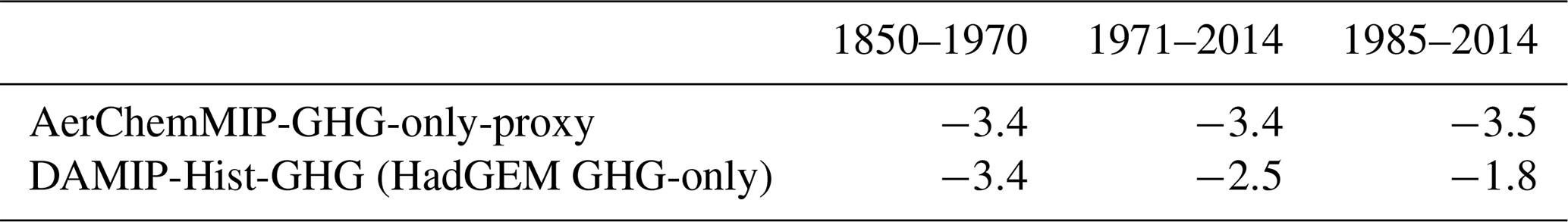
Table 4 shows λ values for different time periods. The AerChemMIP-GHG-only-proxy estimates are consistent across the different periods with values ranging between −3.4 and −3.5 W m−2 K−1. The DAMIP-Hist-GHG (HadGEM-based) value for 1850–1970 (−3.4 W m−2 K−1) is also consistent with these values, whereas the DAMIP-Hist-GHG estimates for the 1971–1985 and 1985–2014 periods are quite different (−2.5 and −1.8 W m−2 K−1). It has been noted previously that cloud feedback magnitudes can vary over time due to natural variability (Armour et al., 2013; Zhou et al., 2016; Andrews et al., 2018), and the HadGEM results may be indicative of such natural variability. Given the consistency of the UKESM1 results, we therefore choose the 1985–2014 λ value of −3.5 W m−2 K−1 for AerChemMIP-GHG-only-proxy since this is the period of interest when comparing with observations and noting that the HadGEM-based value was similar to this for the longer 1850–1970 period; the longer period is likely to reduce uncertainties from short-term variability. Using the larger-magnitude λ values from AerChemMIP-GHG-only-proxy also leads to an upper limit on the estimate of the temperature-bias effect (see below).
Table 4λ values (W m−2 K−1; see Eq. 5) for the UKESM-based (AerChemMIP-piAer) and HadGEM-based (DAMIP-Hist-GHG) greenhouse gas-only simulations (or proxies) for three different time periods.
Multiplying λ by the difference between the observed and modelled ΔT values (i.e. ΔTobserved−ΔTmodel) gives an estimate of the correction to the modelled ΔFSW↑ that is needed to estimate the ΔFSW↑ from cloud feedbacks that would be produced by using the observed temperature trend in place of the modelled one
For the 1985–2014 period, the corrected estimate () for UKESM1 is −3.6 W m−2 (corrected from −5.0 W m−2) and for HadGEM it is −3.1 W m−2 (from −4.5 W m−2). These are closer to the observed value of −1.7 W m−2 but are still considerably too negative. This suggests that either the model cloud feedback (λ) is too strong or the aerosol forcing is too strong. Either of these scenarios would cause a temperature increase that is too steep and hence are also consistent with these factors playing a role in causing the too-large temperature increase. We also note here that using the smaller-magnitude λ values from DAMIP-Hist-GHG would lead to a smaller correction and hence would strengthen this conclusion.
A caveat here is that it has been shown that the specific global pattern of SSTs that occurred in reality is likely to have influenced the magnitude of cloud feedbacks and the climate sensitivity (Armour et al., 2013; Zhou et al., 2016; Andrews et al., 2018) in the real world; this is known as the “pattern effect”. Thus it could be the case that the model cloud feedback response (i.e. λ), and by extension the model climate sensitivity, to a given pattern and magnitude of SST changes is reasonable, but the model is not capturing the correct pattern of SSTs, and hence this is why the FSW↑ trend is too steep. Figures 13 and 14 also show FSW↑ results from a single-member atmosphere-only (UKESM-AMIP) simulation where observed SSTs and sea-ice concentrations are imposed (see Sect. 2.2.3 for more details). It is clear that this run better matches the observed FSW↑ time series and trend, although the trend is still steeper than that observed. Figure 14 shows that the trend from the atmosphere-only run is actually very similar to the estimates made in the previous paragraph where we used the observed ΔT to correct the ΔFSW↑ (converted to a trend for Fig. 14) of the all-emissions runs (UKESM1 and HadGEM). This hints that the magnitude of the SST change may be more important than the spatial pattern for ΔFSW↑ in the N. Atlantic, leaving open the possibility that the cloud feedbacks or aerosol forcing in the model are incorrect. However, the uncertainties are large and further work is needed to determine this.
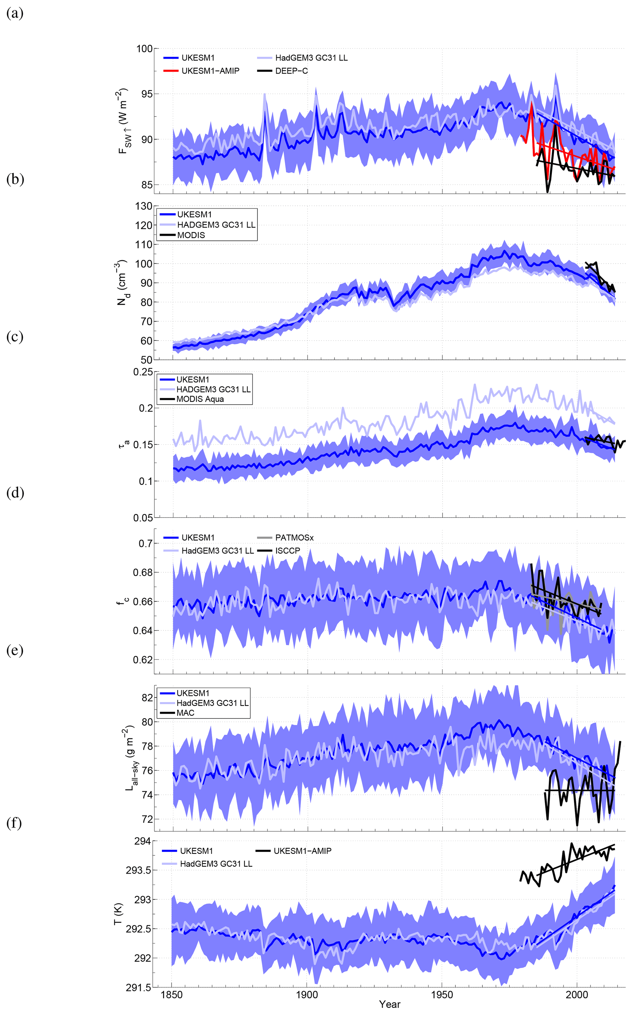
Figure 13Same as for Fig. 2 except showing observations and trend lines that coincide with the observations for the post-1985 period. NB: the PATMOSx and ISCCP cloud fraction values are provided as anomalies from the global mean only, and so the absolute values are uncertain. An arbitrary value of 0.66 was chosen to match the model values in the early part of the time series.
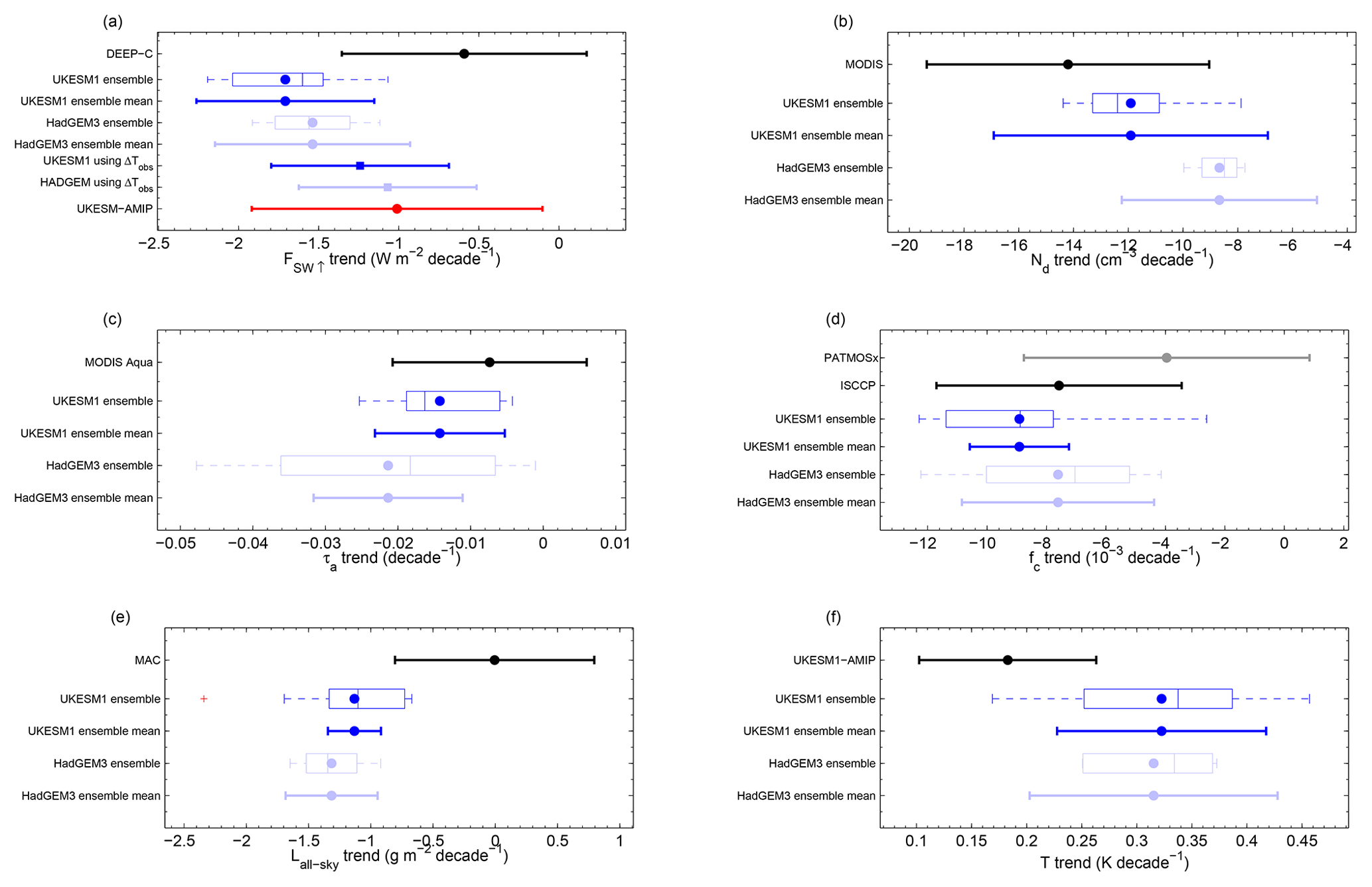
Figure 14Model trends compared to observed trends for time periods chosen to match the available observations: 1985–2014 for DEEP-C FSW↑ observations; 2003–2014 for MODIS Nd and MODIS τa; 1983–2009 for PATMOSx and ISCCP fc; 1988–2014 for MAC LWP; 1985–2014 for the surface temperature UKESM atmosphere-only (AMIP) dataset (more data is available for surface temperature, but this period was chosen to coincide with the FSW↑ time period). For FSW↑ in (a), estimates of the model trend that would occur if the model surface temperature was correct (i.e. equal to the observed temperatures) are also shown (“using ΔTobs”; in Eq. 6). For the models, box and whisker plots of the trends across all ensemble members are shown along with the trend from the ensemble mean time series and its uncertainty. The box and whisker plots show the minimum and maximum as whiskers (or errors bars), except when there are outliers when the error bars are the minimum and maximum of the non-outlier values. Outliers are values that are more than 1.5 times the interquartile range away from the bottom or top of the box and are represented as plus signs. The box edges are the 25th and 75th percentiles, the line within the box is the median and the filled circle is the mean.
In this study we used the HadGEM global coupled climate model and the UKESM1 Earth system model to explore the factors driving historical changes in FSW↑ for the North Atlantic region for ocean grid boxes that contained little sea ice. We found that there is a positive trend in FSW↑ between 1850 and 1970 and then a negative trend until 2014. The analysis shows that the pre-1970 trend is mainly driven by an increase in cloud droplet concentrations (Nd) due to increases in aerosol emissions, and the trend in the later period is mainly driven by a decrease in cloud fraction, likely due to cloud feedbacks caused by greenhouse gas-induced warming.
We also examined the relative effects of aerosol radiative forcing and climate feedbacks on the change in FSW↑. In the pre-1970 period, aerosol-induced cooling and greenhouse gas warming roughly counteracted each other so that there was little cloud feedback effect. Therefore, in this period aerosol forcing is the dominant cause of changes in FSW↑. However, in the post-1970 period the warming from greenhouse gases intensified, leading to a large warming over the North Atlantic and reduction in FSW↑ from cloud feedbacks. Combined with a reduction in aerosol forcing during this period, this led to temperature feedbacks dominating over the aerosol forcing. This is summarized in the schematic of Fig. 15. These results suggest that it is unfeasible to use the post-1970 period (during which there are useful satellite observations) to evaluate and constrain ACIs but that cloud feedbacks might be usefully evaluated, although it may be possible to identify smaller regions or specific times during the satellite era when the aerosol effects are stronger, e.g. when temperature changes are small.
Comparisons to satellite observations between 1985 and 2014 indicate that the model reduction in FSW↑ is too strong for both UKESM1 and HadGEM. The simulated increase in temperature during this period is also too strong. We analysed the extent to which the too-strong temperature trend could explain the excess ΔFSW↑ via cloud feedbacks. However, we find that the bias in temperature trend can only account for part of the ΔFSW↑ discrepancy given the estimated model feedback strength (). This suggested that UKESM1 and HadGEM have positive biases in λ or that the negative aerosol effective radiative forcings are too strong (a too-strong aerosol forcing would produce a positive bias in the temperature increase during the 1985–2014 period because aerosol emissions declined). A λ value that is too negative (too strong a cloud feedback) would directly impact the equilibrium climate sensitivity of the model (producing too much warming for a given forcing). Hence, biases in either the aerosol forcing or the feedback strength would have large implications for future climate projections for these models.
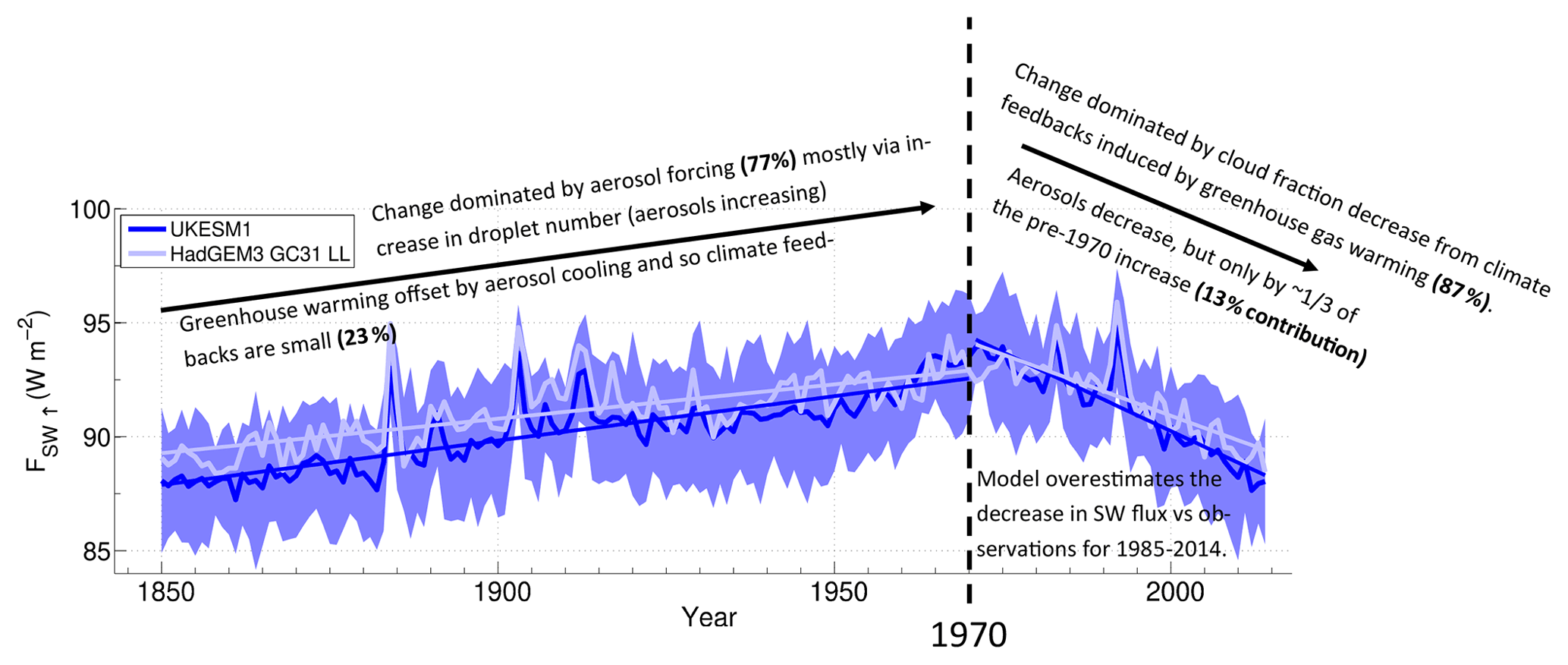
Figure 15Schematic showing the main influences on the determination of the change in FSW↑ during the pre-1970 and post-1970 periods. The quoted percentages are the percentage contributions to ΔFSW↑ from aerosol forcing and climate feedbacks for the two periods.
The analysis also hints that the pattern effect, whereby a particular spatial pattern of SSTs has a large influence on λ and climate sensitivity (Armour et al., 2013; Zhou et al., 2016; Andrews et al., 2018), is not having a large influence on λ for the North Atlantic region. This conclusion is based on the result that ΔFSW↑ from the domain-mean time series for the 1985–2014 period from a simulation that used observed SSTs and sea ice (the atmosphere-only simulation) was similar to estimates made using the UKESM1 and HadGEM coupled model data with the surface temperature changes from the domain-mean time series substituted for the observed temperature change; this suggests that it is the magnitude of the temperature change rather than the spatial pattern that leads to a difference in ΔFSW↑ between the coupled and the atmosphere-only simulations for the North Atlantic. However, the result may not extend to other regions, and uncertainties are large; further work is required to clarify this. Even if there was a large pattern effect, this would still require an explanation of why the model SST trends in the N. Atlantic were too steep and why the model SST pattern was incorrect. It is possible that the natural SST pattern exhibits a high degree of variability such that it might be difficult for a model to simulate the observed pattern, which may have been a low-probability event. We also note that some of the ensemble members did have reasonable N. Atlantic SST trends. On the other hand, the lack of SST agreement could indicate model issues.
If the model cloud feedback strength is too large, then the conclusion (based on the model results) that feedbacks are the dominant cause of the change in FSW↑ during the post-1970 period in the real world would be weakened. However, for the post-1970 period, the ΔFSW↑ value from feedbacks would have to change from −5.4 to −0.83 W m−2 in order for the feedback and aerosol forcing effects to be equal. Therefore, the conclusion is likely to remain robust. On the other hand, if the model aerosol forcing is too large, then using the correct aerosol forcing would enhance the ratio between cloud feedback and aerosol forcing and hence strengthen the conclusions. Furthermore, the strength of the aerosol forcing was decreased during UKESM1 model development (Mulcahy et al., 2018), showing that an excessive forcing strength is a long-standing concern of the model developers.
A recent paper (Dong et al., 2023) examined the individual effects of changes in SSTs/sea-ice extent (SIE), aerosol emissions and GHG emissions for a similar region to that studied here. They used the Met Office GA6.0 atmosphere and land model (Walters et al., 2017), which is an older version of the climate model used in this study. They used atmosphere-only simulations with SSTs taken from observations and examined differences between 2000–2015 time averages and 1980–1985 time averages, which is within the post-1970 analysed in our paper. They focused on the June, July and August (JJA) period. Their results showed that aerosol emission changes dominated the change in downwelling surface solar radiation (SSR) with little influence from SSTs/SIE or GHGs. The lack of influence from SSTs/SIE for that period is in contrast to our results where the cloud feedbacks (driven by SST changes) dominated over aerosol forcing in terms of producing changes in FSW↑ (and presumably SSR too). This difference in results could be due to a number of reasons. One is their use of observed SSTs in contrast to our simulations where the SSTs were predicted by the coupled ocean model. We showed earlier that the SST trends in our coupled model simulations for the post-1970 period were too strong, although correcting for that bias did not change our conclusions. Another potential reason is that there have been a number of advancements of the model between the version used in Dong et al. (2023) and that used in our paper. Those changes are likely to have affected the model feedback responses as well as the aerosol responses; hence, a different balance of aerosol forcing to feedbacks is perhaps expected. Finally, they focused on the JJA season, whereas we used annual averages. Further work is recommended to determine the reasons for these differences as well as to examine differences amongst various other models.
A final interesting implication that follows from our results is that the appearance of coincident peaks in the Nd and FSW↑ time series from the UKESM1 and HadGEM models at around 1970 is due to chance. The decrease in FSW↑ after 1970 is almost entirely caused by the growing effects of greenhouse gas emissions on the larger-scale atmospheric and/or ocean circulation rather than the decrease in aerosols that also starts around 1970. Hence if the greenhouse gas-related effects were shifted to earlier or later in the time series (e.g. due to the rapid increase in greenhouse gas emissions occurring earlier or later), we would expect the decline in FSW↑ to occur correspondingly earlier or later such that the peaks would no longer be coincident. This can be contrasted to the situation over land where the turning point in surface SW flux has been associated with a decline in aerosol emissions (Wild et al., 2005).
A1 North Atlantic time series for HadGEM
Figure A1 shows the time series of FSW↑ and the cloud variables expressed as an anomaly relative to the 1850–1859 mean for the DAMIP experiments. This is similar to the AerChemMIP proxy time series shown in Fig. 6 except that for the DAMIP experiments the different emission types (aerosol, greenhouse gases and natural emissions) were applied individually, and so there is no need to approximate the effects of greenhouse gas-only and aerosol-only emissions as for AerChemMIP (see Sect. 2.2.2). Aerosol emissions (DAMIP-Hist-Aer) cause an increase in FSW↑ over time, whereas greenhouse gas emissions (DAMIP-Hist-GHG) cause a decrease. Natural aerosols (DAMIP-Hist-Nat) produce no trend over the historical period. The sum of the FSW↑ perturbations from the single-emissions runs matches the total from the HadGEM run (with all emissions) reasonably well, suggesting that the main forcing agents are accounted for and that the effects of the individual forcing agents can be combined in a linear sum to approximate the overall change in the full model.
Table A1Same as for Table 1 except for the HadGEM model and DAMIP experiment runs.
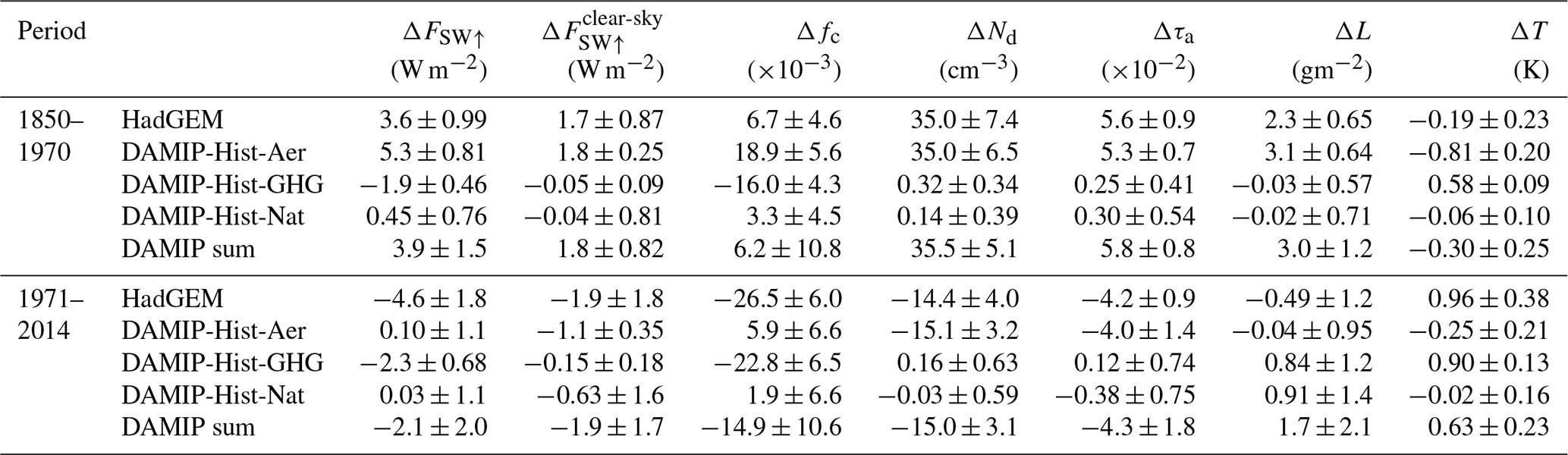
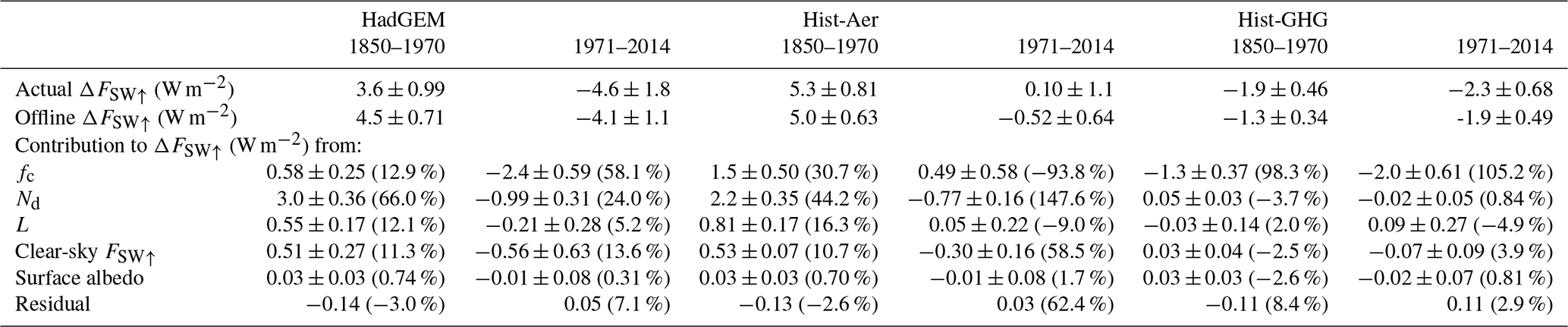
Table A3Same as for Table 3 except for the HadGEM-based DAMIP experiments.
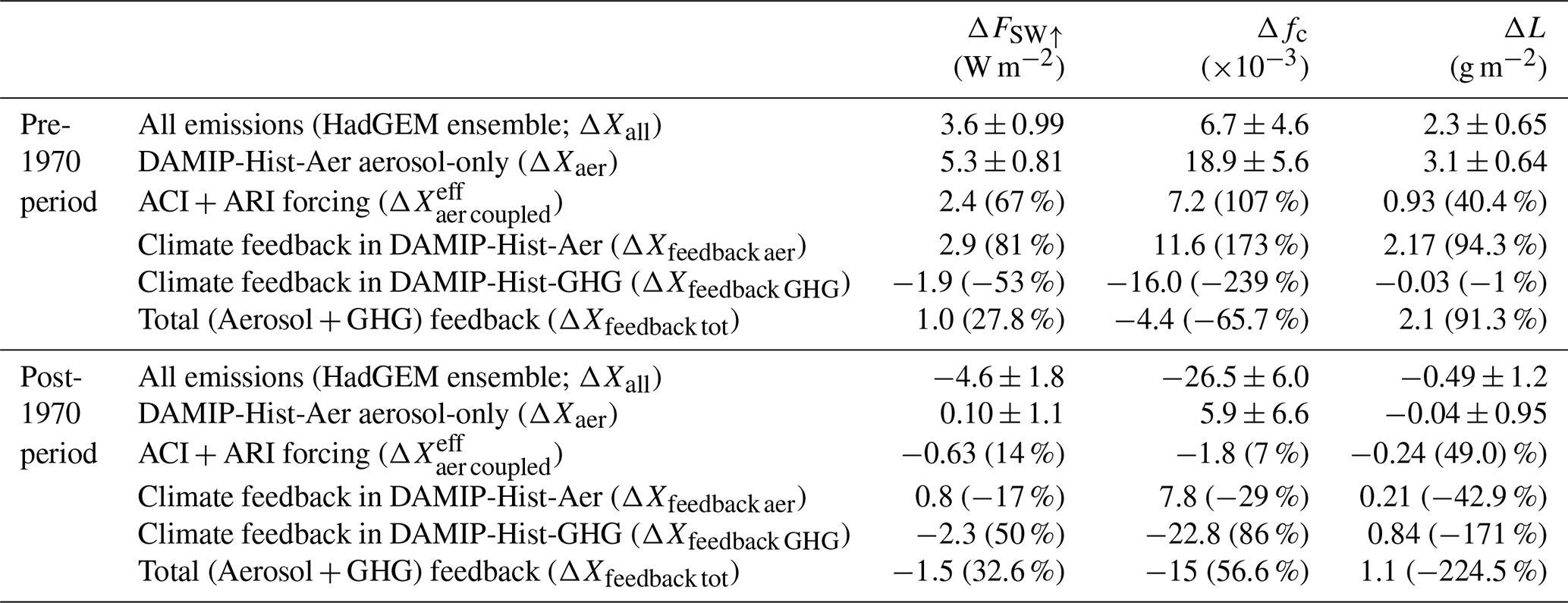

Figure A1Same as for Fig. 6 except for the various single-forcing DAMIP simulations. Lines are shown for the HadGEM-GC3.1 model (which is the model used for the DAMIP experiments) with all forcings applied, the aerosol only forcing DAMIP run (DAMIP-Hist-Aer), the greenhouse gas-only forcing run (DAMIP-Hist-GHG), the natural only forcing run (DAMIP-Hist-Nat), the sum of the perturbations from all of the single forcing runs (DAMIP-linear-sum) and the estimate of the aerosol-only emissions perturbations calculated by subtracting the greenhouse gas-only values from the all-emissions HadGEM values (DAMIP aerosol proxy).
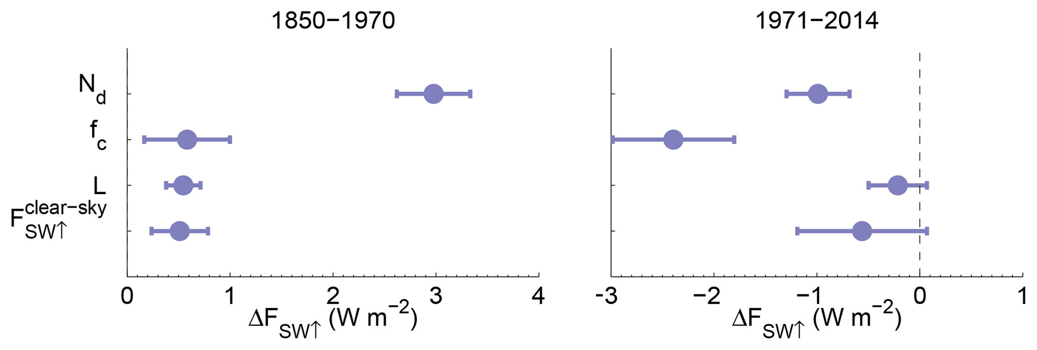
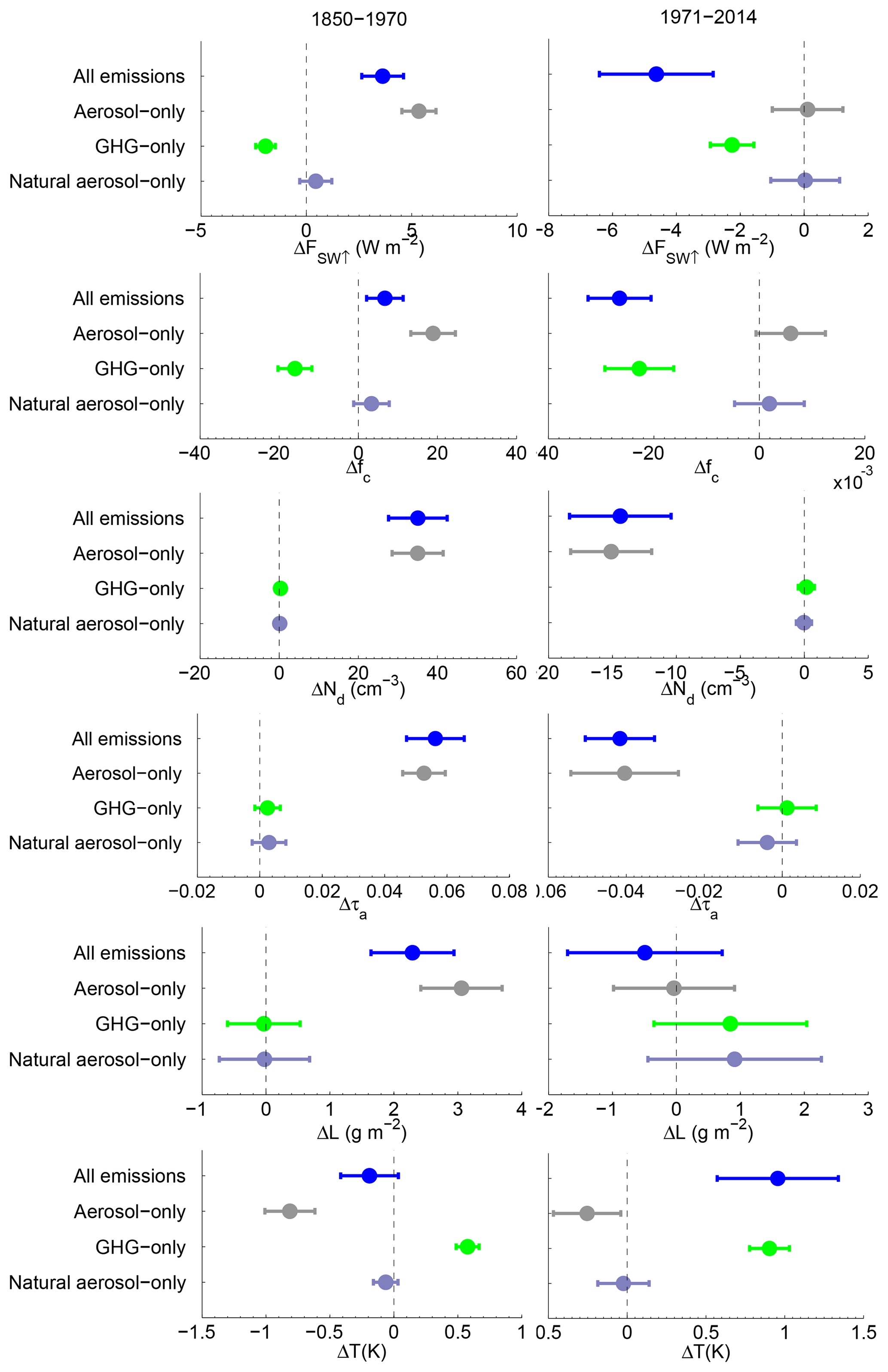
Figure A3Same as for Fig. 7 except for the DAMIP and HadGEM simulations. A natural aerosol-only bar is now shown from the DAMIP-Hist-Nat experiment.
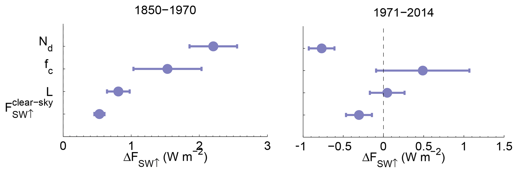
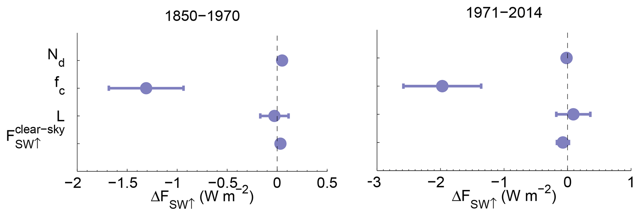
Figure A5Same as for Fig. A5 except for the greenhouse gas-only emissions run (DAMIP-Hist-GHG).
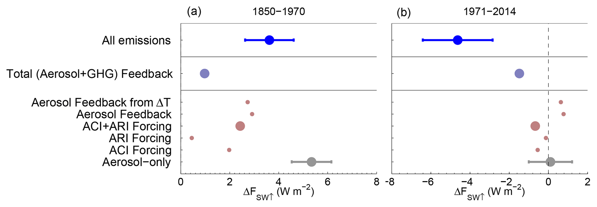
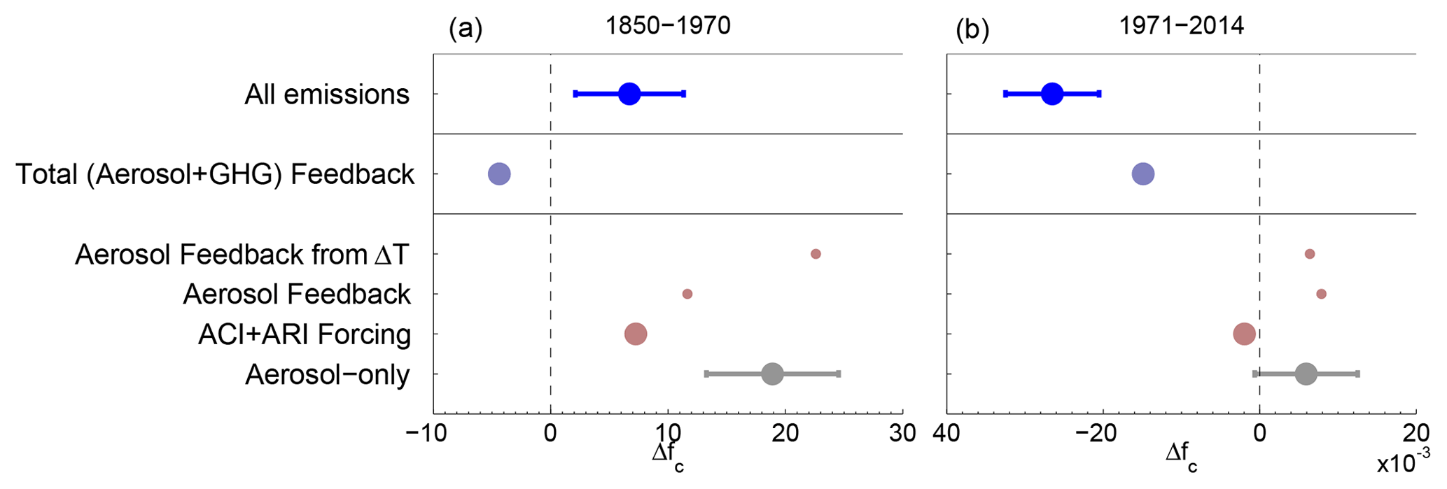
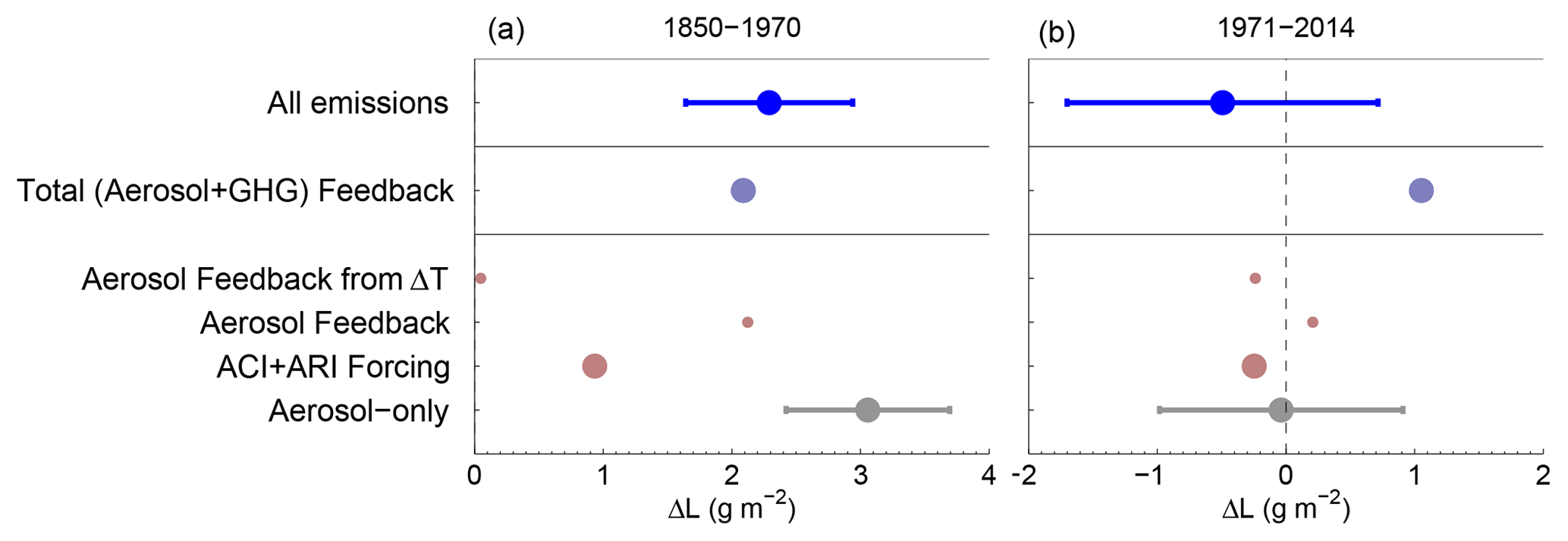
A2 Decomposing the FSW↑ trends in HadGEM into contributions from individual variables
The results of the offline radiative calculations to quantify the effect of changes in cloud variables to the change in FSW↑ for the HadGEM model (Fig. A2) are very similar to those from UKESM1 with Nd changes contributing the most to ΔFSW↑ for the pre-1970 period and fc changes contributing the most for the post-1970 period.
A3 Quantifying the effects of individual emission types on FSW↑ and cloud variable changes
A3.1 Effect of emissions on FSW↑
Figure A3 summarizes the contributions of each emission type to ΔFSW↑ in the two periods for the HadGEM model. For the pre-1970 period, the ΔFSW↑ due to aerosol emissions (estimated from the DAMIP-Hist-Aer simulation) is 5.3 ± 0.81 W m−2 (see Table A1 for the values), which is much larger in magnitude than the reduction in FSW↑ caused by greenhouse gas emissions (from DAMIP-Hist-GHG; −1.9 ± 0.46 W m−2). However, this reduction is still important and shows that in the models with all emissions applied the effect of SW aerosol forcing is offset by around 36 % by opposing greenhouse gas effects.
For the post-1970 period, there is very little contribution from aerosol emissions (0.10 ± 1.1 W m−2) despite a reduction in Nd that is 40 % of the magnitude of the increase of the pre-1970 period. This differs from the results from the AerChemMIP proxy (Fig. 7) where the negative contribution to ΔFSW↑ from the reduction in aerosol emissions during the post-1970 period was estimated to be larger in magnitude than that from the greenhouse gas emissions increase. For the DAMIP experiment, there is a relatively large negative contribution from greenhouse gas emissions (−2.3 ± 0.68 W m−2) for the post-1970 period. For both periods, there is very little contribution to ΔFSW↑ from natural emissions, which justifies the assumption that aerosols and greenhouse gases are the main drivers of changes in FSW↑ that was made for the AerChemMIP calculations.
A3.2 Effect of emissions on fc, Nd and L
Here we consider how the individual emission types affect the underlying cloud variables that were shown in the previous sections to drive the FSW↑ changes (Fig. A3).
The pre-1970 results for fc for the DAMIP experiments are very similar to those from AerChemMIP with opposing effects on fc from greenhouse gases and aerosols to give little overall fc change. However, post-1970 aerosol emissions actually cause a small increase in fc for DAMIP, which is consistent with the near-zero change in FSW↑ from aerosols. In contrast, for AerChemMIP aerosols caused a decrease in FSW↑ and fc.
The results for changes in L are broadly similar between the DAMIP and AerChemMIP, particularly for the pre-1970 period. However, for the post-1970 period the error bars are quite large, which likely explains any differences.
A3.3 Effect of emissions on surface temperature
For the pre-1970 period, the DAMIP results are similar to the AerChemMIP ones. For the post-1970 period, aerosol emissions in the DAMIP experiment cause the surface temperature to decrease slightly, whereas in AerChemMIP they caused a relatively large increase. This opposing behaviour is consistent with the decrease in FSW↑ caused by aerosols in AerChemMIP and near-zero change in FSW↑ in DAMIP since it is likely that the decrease in FSW↑ in AerChemMIP might cause a warming, but also the warming was shown to cause a decrease in FSW↑ through cloud feedbacks (and vice versa for DAMIP).
A4 Decomposing the FSW↑ trends in the single-emissions experiments into contributions from individual cloud and aerosol variables
A4.1 Aerosol-only emissions
The results for DAMIP-Hist-Aer (Fig. A4) are very similar to those for the AerChemMIP experiments for both periods. Changes in Nd drive the majority of the change in FSW↑ for both periods. Changes in fc and L are of lesser importance and only for the pre-1970 period.
A4.2 Greenhouse gas-only emissions
The results for the DAMIP-Hist-GHG simulations (Fig. A5) are very similar to those from AerChemMIP for both periods.
A5 Aerosol forcing vs. cloud–climate feedbacks
A5.1 Forcing vs. feedbacks for FSW↑
The DAMIP results (Fig. A6) are similar to those from AerChemMIP for the pre-1970 period. However, for the post-1970 period cloud–climate feedbacks in the aerosol-only DAMIP-Hist-Aer simulation drive an increase in FSW↑ (consistent with the decrease in surface temperature) as opposed to a decrease in FSW↑ in AerChemMIP (consistent with the increase in surface temperature). As a result, the overall cloud–climate feedback term driven by the combination of aerosols and greenhouse gases is smaller for DAMIP than for AerChemMIP. However, the overall feedback is still larger than the aerosol radiative forcing for DAMIP/HadGEM.
A5.2 Forcing vs. feedbacks for fc, Nd, L
For the pre-1970 period, the DAMIP results for fc (Fig. A7) are again similar to those from AerChemMIP. For the post-1970 period, the cloud feedbacks cause an increase in fc for DAMIP-Hist-Aer, whereas they caused a decrease in AerChemMIP, which is consistent with the respective changes in temperature.
For the pre-1970 period, the DAMIP results for changes in L (Fig. A8) are similar to those from AerChemMIP. As for AerChemMIP, there is a large estimated change in L due to the cloud–climate feedback term in the aerosol-only run when calculated as the difference between the total change in L and the estimated change from aerosol radiative forcing. Again, though, this feedback term is a lot larger than the feedback term estimated using λ (Eq. 5) from the greenhouse gas-only simulation and ΔT from the aerosol-only simulation. This suggests that this discrepancy is not due to the particular model setup of either UKESM1 or HadGEM and that it is a robust result between the two sets of ensemble runs. We can speculate that the discrepancy might be due to the temperature change in the NA not being the controlling factor for cloud feedbacks onto L (e.g. the temperature change elsewhere may be more important) or that this result is spurious due to the noisy nature of the L time series (Fig. A1). Further research is needed to fully determine the cause.
For the post-1970 period, the overall feedback term for L for HadGEM is positive, whereas it was negative for UKESM1. This is partly driven by a positive feedback term in DAMIP-Hist-Aer (instead of negative in AerChemMIP-aerosol-only-proxy) and a larger feedback term in DAMIP-Hist-GHG than in AerChemMIP-GHG-only-proxy. Again, though, the time series are noisy, and the error bars in Figs. 12 and A7 are large so that confidence in this result is low.
A6 Summary
The HadGEM-based DAMIP results are broadly similar to those from the UKESM1-based AerChemMIP experiments. The most prominent discrepancy is the lack of reduction in FSW↑, fc and surface temperature during the post-1970 period for the DAMIP-Hist-Aer (aerosol-only) ensemble; all of these quantities reduce for the AerChemMIP-aerosol-only-proxy ensemble. Here we can only speculate about possible reasons for this; further work would be needed to draw conclusions. One possibility is that the dedicated aerosol-only DAMIP-Hist-Aer simulation allows for the AMOC to increase in strength until 1970 due to the increase in aerosols over that period, which is a proven effect of aerosol forcing in many models (Menary et al., 2020; Robson et al., 2022). This may prevent a rapid response of the climate in the NA to the post-1970 reduction in aerosols due to inertia in the AMOC perhaps related to ocean heat storage, sea-ice changes, etc. Such effects would not be captured by the estimate of aerosol-only effects from the AerChemMIP-aerosol-only-proxy time series. Another possibility is that the temperature and cloud–climate feedbacks in DAMIP-Hist-Aer are being controlled by changes in aerosols outside of the NA region where aerosols may continue to rise after 1970 (e.g. Asia). This idea is supported by the dominance of cloud feedbacks in determining the change in fc in DAMIP-Hist-Aer for the post-1970 period (Fig. A7). This hypothesis would require an explanation for why this result is not seen in the AerChemMIP-aerosol-only-proxy ensemble, suggesting a non-linearity between the effects of the aerosol-only and greenhouse gas-only simulations in explaining the all-emissions simulation results.
Table B1Same as for Table 2 except for the DAMIP experiments for which a comparison is made of the changes in FSW↑ and the offline radiative calculations for the aerosol-only emissions runs (DAMIP-Hist-Aer) and the estimate of aerosol-only emissions (Aerosol Proxy).
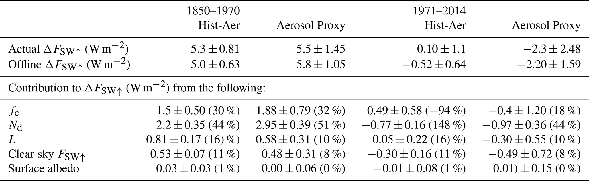
Here we examine the DAMIP single-emission experiment results. The DAMIP experiments may provide some extra insight into the range of possible behaviour given the likely high degree of natural variability. Furthermore, they are based on the HadGEM model rather than the UKESM1 model and hence may display some different behaviour due to the slightly different model physics and settings. We also use the DAMIP experiments in order to validate some of the assumptions made when using the AerChemMIP experiment to approximate single-emission experiments. For example, for the AerChemMIP experiment there is not a true aerosol-only or greenhouse gas-only simulation as there are for the DAMIP experiment. We make the assumption that aerosols and greenhouse gases are the main factors that cause changes in the variables of interest. This means that the AerChemMIP-piAer experiment, where the full set of historical emissions are used except for aerosols for which pre-industrial (PI) emissions are used, would be equivalent to a greenhouse gas-only experiment. A proxy for an aerosol emissions-only experiment was estimated by subtracting the time series from AerChemMIP-piAer from the full emissions simulations. We do the same here for the DAMIP experiment to estimate the accuracy of the AerChemMIP estimate.
Figure A1 shows the proxy aerosol emissions-only time series calculated using the DAMIP results (HadGEM minus DAMIP-Hist-GHG). Comparison of these with the DAMIP-Hist-Aer (true aerosol-only emission experiment) time series shows that the two time series and trends are very similar for all variables, suggesting that the approach used for the calculation of the AerChemMIP-aerosol-only-proxy time series is valid. Table B1 lists those results for FSW↑. The estimated change in FSW↑ (aerosol proxy) for the pre-1970 period is very similar to that from the DAMIP-Hist-Aer experiment suggesting that the proxy works well. For the post-1970 period, the uncertainties in the ΔFSW↑ values are large for DAMIP-Hist-Aer and the proxy, so a comparison is not meaningful.
The table also compares the results of the offline radiative calculations used to estimate the change in FSW↑ and contributions to the changes in FSW↑ from changes in the different cloud variables for the aerosol-only runs. For the pre-1970 period, the aerosol proxy values agree with the DAMIP-Hist-Aer values within the uncertainties, suggesting that the aerosol proxy estimates are sufficient for the AerChemMIP UKESM1 analysis in the main text. The uncertainties are very large for the post-1970 period, and so it is difficult to assess the accuracy of the aerosol proxy method. However, the offline analysis of the contributions to the change in FSW↑ from the change in cloud variables is highlighted as being uncertain in the main text, and is not relied upon for the conclusions that are drawn. We also note that the use of the aerosol proxy only applies for the analysis of the aerosol-only emissions and not the other runs.
Here we utilize output from the same controlled meteorology (nudged) simulations as used in Grosvenor and Carslaw (2020) but for the region of the North Atlantic used in the current paper, to estimate the changes due to aerosol that would occur in the coupled simulations (UKESM1, HadGEM, AerChemMIP and DAMIP) if there were no responses of the large-scale atmospheric or ocean circulation to the aerosol forcing, as was the case in the Grosvenor and Carslaw (2020) simulations where the nudging and use of prescribed SSTs prevents such responses. From the Grosvenor and Carslaw (2020) simulations, changes in various quantities and a change in Nd were calculated, and therefore the sensitivities of the quantities to Nd changes that result from changing from 1850 to 2009 aerosol emissions could also be calculated. We assume that the same sensitivity (when expressed in relative form) would occur in the coupled runs, and we then scale these sensitivities by the ΔNd from the coupled runs for both the pre-1970 period and the post-1970 period to estimate the change in quantity x, where x is either , , fc or L. We express the sensitivities in relative form to account for the different mean values between the simulations of Grosvenor and Carslaw (2020) and the coupled simulations. We find that the aerosol increase in Grosvenor and Carslaw (2020) causes a 59 % increase in Nd, a 1.1 % increase in fc, a 0.82 % increase in L and a 2.7 % increase in FSW↑. The FSW↑ increase was further split into a 2.2% increase from and a 0.5 % increase from again based on the values of these from the nudged runs.
We can then use these percentage changes in the various quantities (denoted ) and the percentage changes in Nd ((%)) to estimate the percentage changes in x that would occur in the coupled simulations if the sensitivity of these quantities to Nd were the same as in the Grosvenor and Carslaw (2020) simulations:
where
Here ΔNd coupled is the change in Nd over the period in question from the coupled run, and is a mean value of Nd from the coupled run used as a baseline for the relative changes. Here we use the mean over the first 5 years of the period. Δxcoupled can then be calculated using
where Δxcoupled(%) comes from Eq. (C1), and is the mean value of x from the coupled run taken over the first 5 years of the period.
The difference between the overall change in a quantity X in the AerChemMIP-aerosol-only-proxy experiment is denoted as ΔXaer and is estimated as the difference between the all-emissions experiment (AerChemMIP-all-emissions) and the GHG-only proxy (AerChemMIP-GHG-only-proxy; see Sect. 2.2.2):
For the AerChemMIP and DAMIP aerosol-only experiments, feedbacks are estimated from the difference between ΔXaer and the change due to aerosol ERF () following Eq. (2). For the AerChemMIP experiments, following Eq. (D1), Eq. (2) becomes
The total feedback is calculated in Figs. 10, 11 and 12 as ΔXfeedback aer plus the feedback from the GHG-only experiment (ΔXfeedback GHG). Since the feedback for the GHG-only experiment is assumed to be ΔXGHG, we have the following (using Eq. D2):
It then follows that the total feedback plus the aerosol forcing is
such that this term is exactly equal to the change in X from the all-emissions run. However, this does not apply to the DAMIP results for which Eq. (D1) does not apply.
Here we consider the implications of the results analysing the SW flux at TOA (FSW↑) for downwelling surface SW fluxes (FSW↓surf). FSW↓surf is important for a variety of reasons; for example, it more directly relates to the energy input into the surface, which may affect ocean heat storage, surface temperatures, the AMOC, etc. From Fig. E1, it is clear that trends in FSW↓surf follow a very similar pattern to those of FSW↑ except in a mirror image. This hints that the results for FSW↑ described in this paper are likely to be applicable to FSW↓surf. However, further analysis would be needed to definitively prove this.
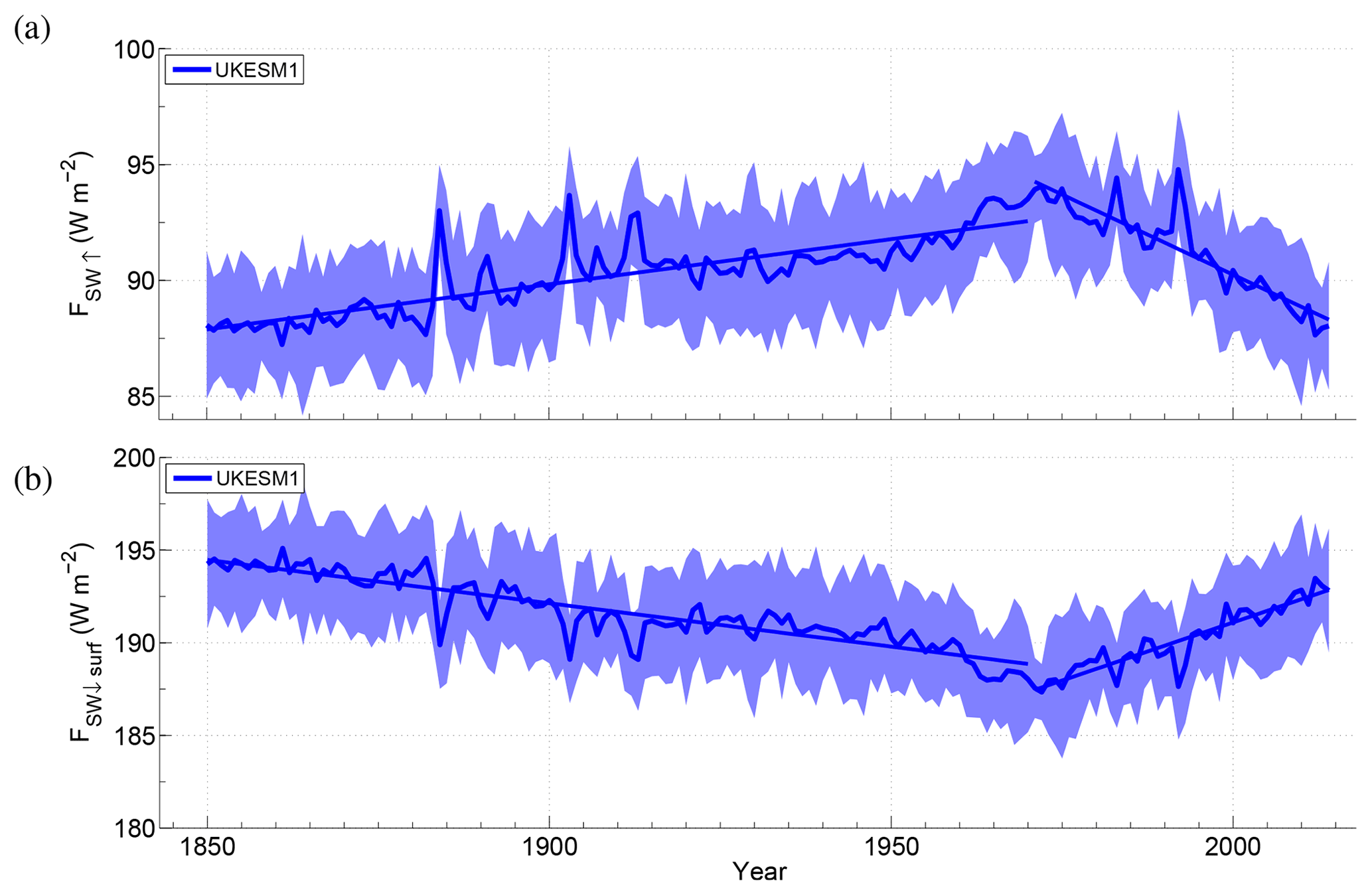
All data used are publically available online. DEEP-C data were obtained from https://doi.org/10.17864/1947.111 (Liu et al., 2017b). MODIS data were obtained from NASA’s Level 1 and Atmosphere Archive and Distribution System (LAADS http://ladsweb.nascom.nasa.gov/, NASA, 2023). Cloud fraction data from PATMOSx and ISCCP were obtained from https://rda.ucar.edu/datasets/ds741.5 (last access: 7 June 2023; Norris and Evan, 2015). MAC-LWP data were obtained from https://disc.gsfc.nasa.gov/datasets/MACLWP_mean_1/summary (last access: 7 June 2023; Elsaesser et al., 2016).
DPG analysed the model data and produced the text and figures. KSC helped to analyse the model output and provided feedback and edits to manuscript drafts.
The contact author has declared that none of the authors has any competing interests.
We acknowledge use of the MONSooN system, a collaborative facility supplied under the Joint Weather and Climate Research Programme, a strategic partnership between the Met Office and the Natural Environment Research Council.
We thank the two anonymous referees who helped to improve the manuscript through their constructive comments.
Publisher’s note: Copernicus Publications remains neutral with regard to jurisdictional claims in published maps and institutional affiliations.
This research has been supported by the Natural Environment Research Council (grant no. NE/N018001/1).
This paper was edited by Yves Balkanski and reviewed by two anonymous referees.
Ackerley, D., Booth, B. B. B., Knight, S. H. E., Highwood, E. J., Frame, D. J., Allen, M. R., and Rowell, D. P.: Sensitivity of Twentieth-Century Sahel Rainfall to Sulfate Aerosol and {CO}2Forcing, J. Climate, 24, 4999–5014, https://doi.org/10.1175/jcli-d-11-00019.1, 2011. a
Ackerman, A. S., Kirkpatrick, M. P., Stevens, D. E., and Toon, O. B.: The impact of humidity above stratiform clouds on indirect aerosol climate forcing, Nature, 432, 1014–1017, https://doi.org/10.1038/nature03174, 2004. a
Albrecht, B. A.: Aerosols, Cloud Microphysics, and Fractional Cloudiness, Science, 80, 1227–1230, 1989. a
Allan, R. P., Liu, C., Loeb, N. G., Palmer, M. D., Roberts, M., Smith, D., and Vidale, P. L.: Changes in global net radiative imbalance 1985–2012, Geophys. Res. Lett., 41, 5588–5597, https://doi.org/10.1002/2014GL060962, 2014a. a, b
Allan, R. P., Liu, C., Loeb, N. G., Palmer, M. D., Roberts, M., Smith, D., and Vidale, P. L.: Changes in global net radiative imbalance 1985-2012, Geophys. Res. Lett., 41, 5588–5597, https://doi.org/10.1002/2014GL060962, 2014b. a
Andrews, T. and Forster, P. M.: CO2 forcing induces semi-direct effects with consequences for climate feedback interpretations, Geophys. Res. Lett., 35, 1–5, https://doi.org/10.1029/2007GL032273, 2008. a
Andrews, T., Gregory, J. M., Paynter, D., Silvers, L. G., Zhou, C., Mauritsen, T., Webb, M. J., Armour, K. C., Forster, P. M., and Titchner, H.: Accounting for Changing Temperature Patterns Increases Historical Estimates of Climate Sensitivity, Geophys. Res. Lett., 45, 8490–8499, https://doi.org/10.1029/2018GL078887, 2018. a, b, c, d
Andrews, T., Andrews, M. B., Bodas-Salcedo, A., Jones, G. S., Kuhlbrodt, T., Manners, J., Menary, M. B., Ridley, J., Ringer, M. A., Sellar, A. A., Senior, C. A., and Tang, Y.: Forcings, Feedbacks, and Climate Sensitivity in HadGEM3-GC3.1 and UKESM1, J. Adv. Model. Earth Syst., 11, 4377–4394, https://doi.org/10.1029/2019MS001866, 2019. a
Archibald, A. T., O'Connor, F. M., Abraham, N. L., Archer-Nicholls, S., Chipperfield, M. P., Dalvi, M., Folberth, G. A., Dennison, F., Dhomse, S. S., Griffiths, P. T., Hardacre, C., Hewitt, A. J., Hill, R. S., Johnson, C. E., Keeble, J., Köhler, M. O., Morgenstern, O., Mulcahy, J. P., Ordóñez, C., Pope, R. J., Rumbold, S. T., Russo, M. R., Savage, N. H., Sellar, A., Stringer, M., Turnock, S. T., Wild, O., and Zeng, G.: Description and evaluation of the UKCA stratosphere–troposphere chemistry scheme (StratTrop vn 1.0) implemented in UKESM1, Geosci. Model Dev., 13, 1223–1266, https://doi.org/10.5194/gmd-13-1223-2020, 2020. a
Armour, K. C., Bitz, C. M., and Roe, G. H.: Time-Varying Climate Sensitivity from Regional Feedbacks, J. Climate, 26, 4518–4534, https://doi.org/10.1175/JCLI-D-12-00544.1, 2013. a, b, c, d
Bai, H., Wang, M., Zhang, Z., and Liu, Y.: Synergetic Satellite Trend Analysis of Aerosol and Warm Cloud Properties ver Ocean and Its Implication for Aerosol-Cloud Interactions, J. Geophys. Res.-Atmos., 125, 1–16, https://doi.org/10.1029/2019JD031598, 2020. a
Berner, A. H., Bretherton, C. S., Wood, R., and Muhlbauer, A.: Marine boundary layer cloud regimes and POC formation in a CRM coupled to a bulk aerosol scheme, Atmos. Chem. Phys., 13, 12549–12572, https://doi.org/10.5194/acp-13-12549-2013, 2013. a
Booth, B. B. B., Dunstone, N. J., Halloran, P. R., Andrews, T., and Bellouin, N.: Aerosols implicated as a prime driver of twentieth-century North Atlantic climate variability, Nature, 484, 228–232, https://doi.org/10.1038/nature10946, 2012. a
Bretherton, C. S., Blossey, P. N., and Uchida, J.: Cloud droplet sedimentation, entrainment efficiency, and subtropical stratocumulus albedo, Geophys. Res. Lett., 34, L03813, https://doi.org/10.1029/2006GL027648, 2007. a
Buckley, M. W. and Marshall, J.: Observations, inferences, and mechanisms of the Atlantic Meridional Overturning Circulation: A review, Rev. Geophys., 54, 5–63, https://doi.org/10.1002/2015RG000493, 2016. a, b, c, d
Carslaw, K. S., Lee, L. A., Reddington, C. L., Pringle, K. J., Rap, A., Forster, P. M., Mann, G. W., Spracklen, D. V., Woodhouse, M. T., Regayre, L. A., and Pierce, J. R.: Large contribution of natural aerosols to uncertainty in indirect forcing, Nature, 503, 67–71, https://doi.org/10.1038/nature12674, 2013. a
Chemke, R., Zanna, L., and Polvani, L. M.: Identifying a human signal in the North Atlantic warming hole, Nat. Commun., 11, 1–7, https://doi.org/10.1038/s41467-020-15285-x, 2020. a
Cherian, R., Quaas, J., Salzmann, M., and Wild, M.: Pollution trends over Europe constrain global aerosol forcing as simulated by climate models, Geophys. Res. Lett., 41, 2176–2181, https://doi.org/10.1002/2013GL058715, 2014. a
Chiang, J. C. H. and Friedman, A. R.: Extratropical Cooling, Interhemispheric Thermal Gradients, and Tropical Climate Change, https://doi.org/10.1146/annurev-earth-042711-105545, 2012. a
Clark, D. B., Mercado, L. M., Sitch, S., Jones, C. D., Gedney, N., Best, M. J., Pryor, M., Rooney, G. G., Essery, R. L. H., Blyth, E., Boucher, O., Harding, R. J., Huntingford, C., and Cox, P. M.: The Joint UK Land Environment Simulator (JULES), model description – Part 2: Carbon fluxes and vegetation dynamics, Geosci. Model Dev., 4, 701–722, https://doi.org/10.5194/gmd-4-701-2011, 2011. a
Collins, W. J., Lamarque, J.-F., Schulz, M., Boucher, O., Eyring, V., Hegglin, M. I., Maycock, A., Myhre, G., Prather, M., Shindell, D., and Smith, S. J.: AerChemMIP: quantifying the effects of chemistry and aerosols in CMIP6, Geosci. Model Dev., 10, 585–607, https://doi.org/10.5194/gmd-10-585-2017, 2017. a
Cox, P. M.: Description of the “TRIFFID” dynamic global vegetation model, Hadley Centre Technical Note, Met Office Hadley Centre, Exeter, Devon, United Kingdom, 2001. a
Dagan, G., Stier, P., and Watson-Parris, D.: Aerosol Forcing Masks and Delays the Formation of the North Atlantic Warming Hole by Three Decades, Geophys. Res. Lett., 47, 1–10, https://doi.org/10.1029/2020GL090778, 2020. a
Dong, B., Sutton, R. T., and Wilcox, L. J.: Decadal trends in surface solar radiation and cloud cover over the North Atlantic sector during the last four decades: drivers and physical processes, Clim. Dynam., 60, 2533–2546, https://doi.org/10.1007/s00382-022-06438-3, 2023. a, b
Dunstone, N. J., Smith, D. M., Booth, B. B. B., Hermanson, L., and Eade, R.: Anthropogenic aerosol forcing of Atlantic tropical storms, Nat. Geosci., 6, 534–539, https://doi.org/10.1038/ngeo1854, 2013. a
Elsaesser, G., O'Dell, C., Lebsock, M., and Teixeira, J.: Multisensor Advanced Climatology Mean Liquid Water Path L3 Monthly 1 degree × 1 degree V1, Greenbelt, MD, USA, Goddard Earth Sciences Data and Information Services Center (GES DISC), EarthData [data set], https://doi.org/10.5067/MEASURES/MACLWPM, 2016. a
Elsaesser, G. S., O'Dell, C. W., Lebsock, M. D., Bennartz, R., Greenwald, T. J., and Wentz, F. J.: The multisensor Advanced climatology of liquid water path (MAC-LWP), J. Climate, 30, 10193–10210, https://doi.org/10.1175/JCLI-D-16-0902.1, 2017. a
Eyring, V., Bony, S., Meehl, G. A., Senior, C. A., Stevens, B., Stouffer, R. J., and Taylor, K. E.: Overview of the Coupled Model Intercomparison Project Phase 6 (CMIP6) experimental design and organization, Geosci. Model Dev., 9, 1937–1958, https://doi.org/10.5194/gmd-9-1937-2016, 2016. a
Feingold, G., Koren, I., Yamaguchi, T., and Kazil, J.: On the reversibility of transitions between closed and open cellular convection, Atmos. Chem. Phys., 15, 7351–7367, https://doi.org/10.5194/acp-15-7351-2015, 2015. a
Forster, P., Alterskjaer, K., Smith, C., Colman, R., Damon Matthews, H., Ramaswamy, V., Storelvmo, T., Armour, K., Collins, W., Dufresne, J.-l., Frame, D., Lunt, D., Mauritsen, T., Watanabe, M., Wild, M., Zhang, H., Masson-Delmotte, V., P. Zhai, Pirani, A., Connors, S., Péan, C., Berger, S., Caud, N., Chen, Y., Goldfarb, L., Gomis, M., Huang, M., Leitzell, K., Lonnoy, E., Matthews, J., Maycock, T., Waterfield, T., Yelekçi, O., Yu, R., and Zhou, B.: The Earth's Energy Budget, Climate Feedbacks, and Climate Sensitivity, in: Climate Change 2021: The Physical Science Basis. Contribution of Working Group I to the Sixth Assessment Report of the Intergovernmental Panel on Climate Change, 923–1054, https://www.ipcc.ch/report/ar6/wg1/downloads/report/IPCC_AR6_WGI_Chapter07.pdf (last access: 7 June 2023), 2021. a
Gillett, N. P., Shiogama, H., Funke, B., Hegerl, G., Knutti, R., Matthes, K., Santer, B. D., Stone, D., and Tebaldi, C.: The Detection and Attribution Model Intercomparison Project (DAMIP v1.0) contribution to CMIP6, Geosci. Model Dev., 9, 3685–3697, https://doi.org/10.5194/gmd-9-3685-2016, 2016. a
Grosvenor, D. P. and Carslaw, K. S.: The decomposition of cloud–aerosol forcing in the UK Earth System Model (UKESM1), Atmos. Chem. Phys., 20, 15681–15724, https://doi.org/10.5194/acp-20-15681-2020, 2020. a, b, c, d, e, f, g, h, i, j, k, l, m, n, o, p
Grosvenor, D. P., Field, P. R., Hill, A. A., and Shipway, B. J.: The relative importance of macrophysical and cloud albedo changes for aerosol-induced radiative effects in closed-cell stratocumulus: insight from the modelling of a case study, Atmos. Chem. Phys., 17, 5155–5183, https://doi.org/10.5194/acp-17-5155-2017, 2017. a
Grosvenor, D. P., Sourdeval, O., Zuidema, P., Ackerman, A., Alexandrov, M. D., Bennartz, R., Boers, R., Cairns, B., Chiu, J. C., Christensen, M., Deneke, H., Diamond, M., Feingold, G., Fridlind, A., Hünerbein, A., Knist, C., Kollias, P., Marshak, A., McCoy, D., Merk, D., Painemal, D., Rausch, J., Rosenfeld, D., Russchenberg, H., Seifert, P., Sinclair, K., Stier, P., van Diedenhoven, B., Wendisch, M., Werner, F., Wood, R., Zhang, Z., and Quaas, J.: Remote Sensing of Droplet Number Concentration in Warm Clouds: A Review of the Current State of Knowledge and Perspectives, Rev. Geophys., 56, 409–453, https://doi.org/10.1029/2017RG000593, 2018. a
Hanna, E., Jones, J. M., Cappelen, J., Mernild, S. H., Wood, L., Steffen, K., and Huybrechts, P.: The influence of North Atlantic atmospheric and oceanic forcing effects on 1900-2010 Greenland summer climate and ice melt/runoff, Int. J. Climatol., 33, 862–880, https://doi.org/10.1002/joc.3475, 2012. a
Held, I. M. and Hou, A. Y.: Nonlinear Axially Symmetric Circulations in a Nearly Inviscid Atmosphere, 37, 515–533, https://doi.org/10.1175/1520-0469(1980)037<0515:nascia>2.0.co;2, 1980. a, b
Hill, A. A., Feingold, G., and Jiang, H.: The Influence of Entrainment and Mixing Assumption on Aerosol Cloud Interactions in Marine Stratocumulus, J. Atmos. Sci., 66, 1450–1464, https://doi.org/10.1175/2008jas2909.1, 2009. a
Hoerling, M., Hurrell, J., Eischeid, J., and Phillips, A.: Detection and Attribution of Twentieth-Century Northern and Southern African Rainfall Change, J. Climate, 19, 3989–4008, https://doi.org/10.1175/jcli3842.1, 2006. a
Holland, D. M., Thomas, R. H., de Young, B., Ribergaard, M. H., and Lyberth, B.: Acceleration of Jakobshavn Isbræ-triggered by warm subsurface ocean waters, Nat. Geosci., 1, 659–664, https://doi.org/10.1038/ngeo316, 2008. a
Knight, J. R., Folland, C. K., and Scaife, A. A.: Climate impacts of the Atlantic Multidecadal Oscillation, Geophys. Res. Lett., 33, L17706, https://doi.org/10.1029/2006gl026242, 2006. a
Kramer, R. J., He, H., Soden, B. J., Oreopoulos, L., Myhre, G., Forster, P. M., and Smith, C. J.: Observational Evidence of Increasing Global Radiative Forcing, Geophys. Res. Lett., 48, 1–11, https://doi.org/10.1029/2020GL091585, 2021. a
Kuhlbrodt, T., Jones, C. G., Sellar, A., Storkey, D., Blockley, E., Stringer, M., Hill, R., Graham, T., Ridley, J., Blaker, A., Calvert, D., Copsey, D., Ellis, R., Hewitt, H., Hyder, P., Ineson, S., Mulcahy, J., Siahaan, A., and Walton, J.: The Low-Resolution Version of HadGEM3 GC3.1: Development and Evaluation for Global Climate, J. Adv. Model. Earth Syst., 10, 2865–2888, https://doi.org/10.1029/2018MS001370, 2018. a, b
Levy, R. C., Mattoo, S., Munchak, L. A., Remer, L. A., Sayer, A. M., Patadia, F., and Hsu, N. C.: The Collection 6 MODIS aerosol products over land and ocean, Atmos. Meas. Tech., 6, 2989–3034, https://doi.org/10.5194/amt-6-2989-2013, 2013. a
Liu, C., Allan, R. P., Berrisford, P., Mayer, M., Hyder, P., Loeb, N., Smith, D., Vidale, P. L., and Edwards, J. M.: Combining satellite observations and reanalysis energy transports to estimate global net surface energy fluxes 1985–2012, J. Geophys. Res., 120, 9374–9389, https://doi.org/10.1002/2015JD023264, 2015. a, b
Liu, C., Allan, R. P., Mayer, M., Hyder, P., Loeb, N. G., Roberts, C. D., Valdivieso, M., Edwards, J. M., and Vidale, P. L.: Evaluation of satellite and reanalysis-based global net surface energy flux and uncertainty estimates, J. Geophys. Res., 122, 6250–6272, https://doi.org/10.1002/2017JD026616, 2017a. a, b
Liu, C. and Allan, R.: Reconstructions of the radiation fluxes at top of atmosphere and net surface energy flux in the period 1985–2015 from DEEP-C project, University of Reading [data set], https://doi.org/10.17864/1947.111, 2017b. a
Lu, J., Vecchi, G. A., and Reichler, T.: Expansion of the Hadley cell under global warming, Geophys. Res. Lett., 34, 2–6, https://doi.org/10.1029/2006GL028443, 2007. a, b
Manabe, S. and Stouffer, R. J.: Century-scale effects of increased atmospheric C02 on the ocean-atmosphere system, Nature, 364, 215–218, https://doi.org/10.1038/364215a0, 1993. a
McCarthy, G. D., Haigh, I. D., Hirschi, J. J.-M., Grist, J. P., and Smeed, D. A.: Ocean impact on decadal Atlantic climate variability revealed by sea-level observations, Nature, 521, 508–510, https://doi.org/10.1038/nature14491, 2015. a
Menary, M. B., Robson, J., Allan, R. P., Booth, B. B. B., Cassou, C., Gastineau, G., Gregory, J., Hodson, D., Jones, C., Mignot, J., Ringer, M., Sutton, R., Wilcox, L., and Zhang, R.: Aerosol‐Forced AMOC Changes in CMIP6 Historical Simulations, Geophys. Res. Lett., 47, e2020GL088166, https://doi.org/10.1029/2020GL088166, 2020. a, b, c
Mulcahy, J. P., Jones, C., Sellar, A., Johnson, B., Boutle, I. A., Jones, A., Andrews, T., Rumbold, S. T., Mollard, J., Bellouin, N., Johnson, C. E., Williams, K. D., Grosvenor, D. P., and McCoy, D. T.: Improved Aerosol Processes and Effective Radiative Forcing in HadGEM3 and UKESM1, J. Adv. Model. Earth Syst., 10, 2786–2805, https://doi.org/10.1029/2018MS001464, 2018. a
Myhre, G., Shindell, D., Bréon, F.-M., Collins, W., Fuglestvedt, J., Huang, J., Koch, D., Lamarque, J.-F., Lee, D., Mendoza, B., Nakajima, T., Robock, A., Stephens, G., Takemura, T., and Zhang, H.: Anthropogenic and Natural Radiative Forcing, in: Clim. Chang. 2013 Phys. Sci. Basis. Contrib. Work. Gr. I to Fifth Assess. Rep. Intergov. Panel Clim. Chang., edited by: Stocker, T., Qin, D., Plattner, G.-K., Tignor, M., Allen, S., Boschung, J., Nauels, A., Xia, Y., Bex, V., and Midgley, P., vol. 9781107057, 659–740, Cambridge University Press, Cambridge, United Kingdom and New York, NY, USA, https://doi.org/10.1017/CBO9781107415324.018, 2013. a
NASA: LAADS DAAC, Your Source for Level-1 and Atmospheric Data, http://ladsweb.nascom.nasa.gov/ (last access: 7 June 2023), 2023. a
Norris, J. R. and Evan, A. T.: Cloud Properties from ISCCP and PATMOS-x Corrected for Spurious Variability Related to Changes in Satellite Orbits, Instrument Calibrations, and Other Factors, Research Data Archive at the National Center for Atmospheric Research, Computational and Information Systems Laboratory, NCAR [data set], https://doi.org/10.5065/D62J68XR, 2015. a
Norris, J. R., Allen, R. J., Evan, A. T., Zelinka, M. D., O'Dell, C. W., and Klein, S. A.: Evidence for climate change in the satellite cloud record, Nature, 536, 72–75, https://doi.org/10.1038/nature18273, 2016. a, b, c, d
O'Connor, F. M., Abraham, N. L., Dalvi, M., Folberth, G. A., Griffiths, P. T., Hardacre, C., Johnson, B. T., Kahana, R., Keeble, J., Kim, B., Morgenstern, O., Mulcahy, J. P., Richardson, M., Robertson, E., Seo, J., Shim, S., Teixeira, J. C., Turnock, S. T., Williams, J., Wiltshire, A. J., Woodward, S., and Zeng, G.: Assessment of pre-industrial to present-day anthropogenic climate forcing in UKESM1, Atmos. Chem. Phys., 21, 1211–1243, https://doi.org/10.5194/acp-21-1211-2021, 2021. a
Painemal, D. and Zuidema, P.: Assessment of MODIS cloud effective radius and optical thickness retrievals over the Southeast Pacific with VOCALS-REx in situ measurements, J. Geophys. Res., 116, D24206, https://doi.org/10.1029/2011JD016155, 2011. a
Robson, J., Ortega, P., and Sutton, R.: A reversal of climatic trends in the North Atlantic since 2005, Nat. Geosci., 9, 513–517, https://doi.org/10.1038/ngeo2727, 2016. a
Robson, J., Sutton, R. T., Archibald, A., Cooper, F., Christensen, M., Gray, L. J., Holliday, N. P., Macintosh, C., McMillan, M., Moat, B., Russo, M., Tilling, R., Carslaw, K., Desbruyères, D., Embury, O., Feltham, D. L., Grosvenor, D. P., Josey, S., King, B., Lewis, A., McCarthy, G. D., Merchant, C., New, A. L., O'Reilly, C. H., Osprey, S. M., Read, K., Scaife, A., Shepherd, A., Sinha, B., Smeed, D., Smith, D., Ridout, A., Woollings, T., and Yang, M.: Recent multivariate changes in the North Atlantic climate system, with a focus on 2005–2016, Int. J. Climatol., 38, 5050–5076, https://doi.org/10.1002/joc.5815, 2018. a
Robson, J., Menary, M. B., Sutton, R. T., Mecking, J., Gregory, J. M., Jones, C., Sinha, B., Stevens, D. P., and Wilcox, L. J.: The role of anthropogenic aerosol forcing in the 1850–1985 strengthening of the AMOC in CMIP6 historical simulations, J. Climate, 1, 1–48, https://doi.org/10.1175/JCLI-D-22-0124.1, 2022. a, b
Santer, B. D., Wigley, T. M., Boyle, J. S., Gaffen, D. J., Hnilo, J. J., Nychka, D., Parker, D. E., and Taylor, K. E.: Statistical significance of trends and trend differences in layer-average atmospheric temperature time series, J. Geophys. Res.-Atmos., 105, 7337–7356, https://doi.org/10.1029/1999JD901105, 2000. a
Seethala, C. and Horváth, Á.: Global assessment of {AMSR-E and MODIS} cloud liquid water path retrievals in warm oceanic clouds, J. Geophys. Res., 115, D13202, https://doi.org/10.1029/2009JD012662, 2010. a
Seidel, D. J., Fu, Q., Randel, W. J., and Reiohler, T. J.: Widening of the tropical belt in a changing climate, Nat. Methods, 1, 21–24, https://doi.org/10.1038/ngeo.2007.38, 2008. a, b
Seinfeld, J. H. and Pandis, S. N.: Atmospheric chemistry and physics : from air pollution to climate change, 1152 pp., Hoboken, N.J. J. Wiley, 2 Edn., ISBN 978-1-118-94740-1, 2006. a
Sellar, A. A., Jones, C. G., Mulcahy, J., Tang, Y., Yool, A., Wiltshire, A., O'Connor, F. M., Stringer, M., Hill, R., Palmieri, J., Woodward, S., Mora, L., Kuhlbrodt, T., Rumbold, S., Kelley, D. I., Ellis, R., Johnson, C. E., Walton, J., Abraham, N. L., Andrews, M. B., Andrews, T., Archibald, A. T., Berthou, S., Burke, E., Blockley, E., Carslaw, K., Dalvi, M., Edwards, J., Folberth, G. A., Gedney, N., Griffiths, P. T., Harper, A. B., Hendry, M. A., Hewitt, A. J., Johnson, B., Jones, A., Jones, C. D., Keeble, J., Liddicoat, S., Morgenstern, O., Parker, R. J., Predoi, V., Robertson, E., Siahaan, A., Smith, R. S., Swaminathan, R., Woodhouse, M. T., Zeng, G., and Zerroukat, M.: UKESM1: Description and evaluation of the UK Earth System Model, J. Adv. Model. Earth Syst., 11, 1–46, https://doi.org/10.1029/2019ms001739, 2019. a, b, c
Smith, D. M., Eade, R., Dunstone, N. J., Fereday, D., Murphy, J. M., Pohlmann, H., and Scaife, A. A.: Skilful multi-year predictions of Atlantic hurricane-frequency, Nat. Geosci., 3, 846–849, https://doi.org/10.1038/ngeo1004, 2010. a
Srokosz, M., Baringer, M., Bryden, H., Cunningham, S., Delworth, T., Lozier, S., Marotzke, J., and Sutton, R.: Past, present, and future changes in the atlantic meridional overturning circulation, B. Am. Meteorol. Soc., 93, 1663–1676, https://doi.org/10.1175/BAMS-D-11-00151.1, 2012. a, b
Stevens, B., Cotton, W. R., Feingold, G., and Moeng, C.-H.: Large-Eddy Simulations of Strongly Precipitating, Shallow, Stratocumulus-Topped Boundary Layers, J. Atmos. Sci., 55, 3616–3638, https://doi.org/10.1175/1520-0469(1998)055<3616:lesosp>2.0.co;2, 1998. a
Sutton, R. T. and Dong, B.: Atlantic Ocean influence on a shift in European climate in the 1990s, Nat. Geosci., 5, 788–792, https://doi.org/10.1038/ngeo1595, 2012. a
Sutton, R. T. and Hodson, D. L. R.: Atlantic Ocean Forcing of North American and European Summer Climate, Science, 80, 115–118, https://doi.org/10.1126/science.1109496, 2005. a
Twomey, S.: The Influence of Pollution on the Shortwave Albedo of Clouds, J. Atmos. Sci., 34, 1149–1152, https://doi.org/10.1175/1520-0469(1977)034<1149:tiopot>2.0.co;2, 1977. a
Walters, D., Boutle, I., Brooks, M., Melvin, T., Stratton, R., Vosper, S., Wells, H., Williams, K., Wood, N., Allen, T., Bushell, A., Copsey, D., Earnshaw, P., Edwards, J., Gross, M., Hardiman, S., Harris, C., Heming, J., Klingaman, N., Levine, R., Manners, J., Martin, G., Milton, S., Mittermaier, M., Morcrette, C., Riddick, T., Roberts, M., Sanchez, C., Selwood, P., Stirling, A., Smith, C., Suri, D., Tennant, W., Vidale, P. L., Wilkinson, J., Willett, M., Woolnough, S., and Xavier, P.: The Met Office Unified Model Global Atmosphere 6.0/6.1 and JULES Global Land 6.0/6.1 configurations, Geosci. Model Dev., 10, 1487–1520, https://doi.org/10.5194/gmd-10-1487-2017, 2017. a
Wang, C., Soden, B. J., Yang, W., and Vecchi, G. A.: Compensation Between Cloud Feedback and Aerosol-Cloud Interaction in CMIP6 Models, Geophys. Res. Lett., 48, 1–10, https://doi.org/10.1029/2020GL091024, 2021. a
Wild, M., Gilgen, H., Roesch, A., Ohmura, A., Long, C. N., Dutton, E. C., Forgan, B., Kallis, A., Russak, V., and Tsvetkov, A.: From dimming to brightening: Decadal changes in solar radiation at earth's surface, Science, 80, 847–850, https://doi.org/10.1126/science.1103215, 2005. a
Williams, K. D., Copsey, D., Blockley, E. W., Bodas-Salcedo, A., Calvert, D., Comer, R., Davis, P., Graham, T., Hewitt, H. T., Hill, R., Hyder, P., Ineson, S., Johns, T. C., Keen, A. B., Lee, R. W., Megann, A., Milton, S. F., Rae, J. G., Roberts, M. J., Scaife, A. A., Schiemann, R., Storkey, D., Thorpe, L., Watterson, I. G., Walters, D. N., West, A., Wood, R. A., Woollings, T., and Xavier, P. K.: The Met Office Global Coupled Model 3.0 and 3.1 (GC3.0 and GC3.1) Configurations, J. Adv. Model. Earth Syst., 10, 357–380, https://doi.org/10.1002/2017MS001115, 2017. a, b
Wiltshire, A. J., Duran Rojas, M. C., Edwards, J. M., Gedney, N., Harper, A. B., Hartley, A. J., Hendry, M. A., Robertson, E., and Smout-Day, K.: JULES-GL7: the Global Land configuration of the Joint UK Land Environment Simulator version 7.0 and 7.2, Geosci. Model Dev., 13, 483–505, https://doi.org/10.5194/gmd-13-483-2020, 2020. a
Woollings, T., Franzke, C., Hodson, D. L. R., Dong, B., Barnes, E. A., Raible, C. C., and Pinto, J. G.: Contrasting interannual and multidecadal NAO variability, Clim. Dynam., 45, 539–556, https://doi.org/10.1007/s00382-014-2237-y, 2015. a
Yool, A., Popova, E. E., and Anderson, T. R.: MEDUSA-2.0: an intermediate complexity biogeochemical model of the marine carbon cycle for climate change and ocean acidification studies, Geosci. Model Dev., 6, 1767–1811, https://doi.org/10.5194/gmd-6-1767-2013, 2013. a
Yu, S. and Pritchard, M. S.: A strong role for the AMOC in partitioning global energy transport and shifting ITCZ position in response to latitudinally discrete solar forcing in CESM1.2, J. Climate, 32, 2207–2226, https://doi.org/10.1175/JCLI-D-18-0360.1, 2019. a
Zhang, R. and Delworth, T. L.: Impact of Atlantic multidecadal oscillations on India/Sahel rainfall and Atlantic hurricanes, Geophys. Res. Lett., 33, L17712, https://doi.org/10.1029/2006gl026267, 2006. a
Zhou, C., Zelinka, M. D., and Klein, S. A.: Impact of decadal cloud variations on the Earth's energy budget, Nat. Geosci., 9, 871–874, https://doi.org/10.1038/ngeo2828, 2016. a, b, c, d
- Abstract
- Introduction
- Methods
- Results
- Comparison with observations
- Discussion and conclusions
- Appendix A: HadGEM DAMIP results
- Appendix B: Testing the assumptions made for AerChemMIP aerosol and greenhouse gas-only proxies
- Appendix C: Estimation of aerosol forcing based on nudged simulations
- Appendix D: Summation of terms in feedback figures
- Appendix E: Implications for surface SW downwelling fluxes
- Data availability
- Author contributions
- Competing interests
- Acknowledgements
- Disclaimer
- Financial support
- Review statement
- References