the Creative Commons Attribution 4.0 License.
the Creative Commons Attribution 4.0 License.
 | 24 Jun 2021
Characterizing model errors in chemical transport modeling of methane: using GOSAT XCH4 data with weak-constraint four-dimensional variational data assimilation
Ilya Stanevich
Dylan B. A. Jones
Kimberly Strong
Martin Keller
Daven K. Henze
Robert J. Parker
Hartmut Boesch
Debra Wunch
Justus Notholt
Christof Petri
Thorsten Warneke
Ralf Sussmann
Matthias Schneider
Frank Hase
Rigel Kivi
Nicholas M. Deutscher
Voltaire A. Velazco
Kaley A. Walker
Feng Deng
We examined biases in the global GEOS-Chem chemical transport model for the period of February–May 2010 using weak-constraint (WC) four-dimensional variational (4D-Var) data assimilation and dry-air mole fractions of CH4 (XCH4) from the Greenhouse gases Observing SATellite (GOSAT). The ability of the observations and the WC 4D-Var method to mitigate model errors in CH4 concentrations was first investigated in a set of observing system simulation experiments (OSSEs). We then assimilated the GOSAT XCH4 retrievals and found that they were capable of providing information on the vertical structure of model errors and of removing a significant portion of biases in the modeled CH4 state. In the WC 4D-Var assimilation, corrections were added to the modeled CH4 state at each model time step to account for model errors and improve the model fit to the assimilated observations. Compared to the conventional strong-constraint (SC) 4D-Var assimilation, the WC method was able to significantly improve the model fit to independent observations. Examination of the WC state corrections suggested that a significant source of model errors was associated with discrepancies in the model CH4 in the stratosphere. The WC state corrections also suggested that the model vertical transport in the troposphere at middle and high latitudes is too weak. The problem was traced back to biases in the uplift of CH4 over the source regions in eastern China and North America. In the tropics, the WC assimilation pointed to the possibility of biased CH4 outflow from the African continent to the Atlantic in the mid-troposphere. The WC assimilation in this region would greatly benefit from glint observations over the ocean to provide additional constraints on the vertical structure of the model errors in the tropics. We also compared the WC assimilation at 4∘ × 5∘ and 2∘ × 2.5∘ horizontal resolutions and found that the WC corrections to mitigate the model errors were significantly larger at 4∘ × 5∘ than at 2∘ × 2.5∘ resolution, indicating the presence of resolution-dependent model errors. Our results illustrate the potential utility of the WC 4D-Var approach for characterizing model errors. However, a major limitation of this approach is the need to better characterize the specified model error covariance in the assimilation scheme.
- Article
(16396 KB) - Full-text XML
- BibTeX
- EndNote


Atmospheric concentrations of methane (CH4), the second most important anthropogenic greenhouse gas, have been rapidly raising since 1850 (Etheridge et al., 1992). However, atmospheric measurements in recent decades show that the rate of CH4 increase in the atmosphere has varied, and its behavior is not well understood (Dlugokencky et al., 2009). Significant effort has been put into characterizing surface emissions of CH4 in order to attribute its recent trends. In this context, a number of satellites have been launched to measure atmospheric CH4 in order to constrain its sources. These include Envisat carrying the Scanning Imaging Absorption Spectrometer for Atmospheric Cartography (SCIAMACHY; Schneising et al., 2011), the Greenhouse Gases Observing Satellite (GOSAT) carrying the Thermal And Near-infrared Sensor for carbon Observation Fourier Transport Spectrometer (TANSO-FTS; Kuze et al., 2009), Sentinel-5p with the Tropospheric Monitoring Instrument (TROPOMI) on board (Veefkind et al., 2012), and the Greenhouse Gases Satellite (GHGSat). Proposed missions include the Methane Remote Sensing Lidar Mission (MERLIN; Kiemle et al., 2014), GOSAT-2 (Nakajima et al., 2017), the Geostationary Carbon Cycle Observatory (GeoCARB; Polonsky et al., 2014), and the recently announced MethaneSat. However, current regional CH4 emissions remain largely uncertain (e.g., Saunois et al., 2016). One of the biggest challenges for reducing uncertainty in emission estimates is the relatively weak signal of emissions in the atmospheric column of CH4, which puts tight requirements on the accuracy of satellite measurements. However, while future satellite instruments and improved spectroscopy are expected to provide better CH4 measurements, errors in the atmospheric models used to simulate CH4 remain poorly characterized. While random model errors can be accounted for in flux inversion analyses, the impact of biases in chemistry and transport are often neglected or accounted for using various ad hoc approaches. In the case of CH4, which is a relatively long-lived gas with an atmospheric lifetime of about 9 years (Prather et al., 2012), chemistry plays a critical role in long-term trends (McNorton et al., 2016), whereas transport, alone or coupled with chemistry, defines how total surface emissions are distributed on a regional scale. Therefore, transport errors, such as those produced by numerical advection schemes, biases and uncertainties of meteorological fields, and parametrization of sub-grid-scale processes, may significantly undermine our ability to use models to relate emissions to atmospheric observations and thus our ability to improve CH4 emission estimates (Prather et al., 2008; Locatelli et al., 2015; Patra et al., 2011).
One potential solution is to apply a bias correction to the model in the context of the inversion analysis. Simple bias correction schemes with uniform or latitudinally dependent bias estimates have been attempted before (Bergamaschi et al., 2009; Fraser et al., 2013; Monteil et al., 2013; Alexe et al., 2015; Locatelli et al., 2015), mostly to correct poor descriptions of the modeled stratosphere. Here we explore the utility of a “weak-constraint” (WC) four-dimensional variational (4D-Var) data assimilation method to characterize forward model errors. In contrast to the traditional “strong-constraint” (SC) 4D-Var method, the WC scheme does not assume that the model evolution is perfect. The WC 4D-Var method was introduced by Sasaki (1970) and used in numerical weather prediction (NWP) models by Derber (1989), Zupanski (1997), and Trémolet (2006, 2007). It was first applied by Keller (2014) in the GEOS-Chem simulation of atmospheric carbon monoxide (CO) to characterize model bias. One of the first attempts to apply bias correction in chemical data assimilation was done in the framework of the suboptimal Kalman filter by Lamarque et al. (2004), who used the bias estimation approach of Dee and Da Silva (1998) to constrain the CO state using measurements from the Measurement of Pollution in the Troposphere (MOPITT) instrument. The study pointed to the possibility of errors in the model vertical transport; however, most of the estimated biases were attributed to poor a priori estimates of CO surface emissions in the model. The major challenge for this type of analysis for CH4 is the limited information available about the global vertical distribution of CH4 in the atmosphere. There are satellite observations that contain information about the CH4 distribution in the middle and upper troposphere, such as the thermal infrared CH4 retrievals from the Tropospheric Emission Spectrometer (TES) on board the NASA Aura satellite (Worden et al., 2012), and in the stratosphere, such as the solar occultation measurements from the Atmospheric Chemistry Experiment Fourier Transform Spectrometer (ACE-FTS; Bernath et al., 2005) on board SCISAT. However, the accuracy of these measurements, based on validation studies (for example, De Mazière et al., 2008; Wecht et al., 2012), may not be sufficient to detect model errors. The most accurate satellite measurements are those of the total dry-air mole fraction of CH4 in the total atmospheric column (XCH4) obtained by TANSO-FTS on board GOSAT. However, these measurements provide less vertical information on CH4 than those from TES and ACE-FTS, although the latter are less sensitive to surface emissions. Highly accurate aircraft or AirCore CH4 profile measurements would be an ideal source of information, but they are limited in space and time. We explore the information content of GOSAT CH4 observations and show that despite being designed to constrain surface emissions, they contain sufficient information to help characterize possible model errors. We assimilate the GOSAT observations using the WC 4D-Var data assimilation approach to estimate biases in GEOS-Chem. This approach is shown to provide a valuable tool for diagnosing and determining the origin of model errors.
This paper is organized as follows. Section 2 gives an overview of the forward model, the observations, and the WC 4D-Var method. It also contains a description of the various sensitivity studies conducted through a series of observing system simulation experiments (OSSEs). In Sect. 3, we present the results of the sensitivity experiments and the results of the assimilation of real GOSAT observations. Section 4 provides an interpretation of the pattern of model biases estimated from the GOSAT assimilation. Finally, conclusions are given in Sect. 5.
2.1 The GEOS-Chem model
For all assimilation experiments we use version v35 of the GEOS-Chem adjoint, which is based on version v8-02-01 of the forward model, with updates up to v9-02 (Henze et al., 2007). The GEOS-Chem chemical transport model (CTM) (http://www.geos-chem.org, last access: 21 May 2021) is driven by archived meteorological fields from the Goddard Earth Observing System (GEOS-5.2.0) produced by the NASA Global Modeling and Assimilation Office (GMAO). The meteorological fields are regridded from their native resolution of 0.5∘ × 0.67∘ with 72 vertical levels to 4∘ × 5∘ and 2∘ × 2.5∘ with 47 vertical levels. The vertical grid spacing in the troposphere varies from about 150 m in the lower part to about 1 km in the upper part. CH4 is advected using the multidimensional flux-form semi-Lagrangian (FFSL) scheme by Lin and Rood (1996). Convection is implemented based on the relaxed Arakawa–Schubert scheme (Moorthi and Suarez, 1992). The model uses a simple treatment of turbulent mixing in the boundary layer by instantaneously mixing species from the surface to the top of the planetary boundary layer (PBL). The GEOS-Chem CH4 sources and sinks used here are described in detail in Wecht et al. (2014). Anthropogenic CH4 sources include emissions from natural gas and oil extraction, coal mining, livestock, landfills, wastewater treatment, rice cultivation, biofuel burning, and other minor sources based on the 2004 anthropogenic inventory from the Emission Database for Global Atmospheric Research (EDGAR) v4.2 (European Commission Joint Research Centre/Netherlands Environmental Assessment Agency, 2009). Natural CH4 sources include wetland emissions after Kaplan (2002) and Pickett-Heaps et al. (2011), termite emissions (Fung et al., 1991), and open fire emissions from the daily Global Fire Emissions Database version 3 (GFED3) (van der Werf et al., 2010; Mu et al., 2011). The CH4 emissions at 4∘ × 5∘ and 2∘ × 2.5∘ resolutions are slightly different due to the dependence of wetland emissions on the meteorological fields. Therefore, for consistency of the analysis of model errors, the emissions were regridded from the coarser to the finer resolution. The main loss of CH4 (about 90 % of the total loss) in the atmosphere is due to oxidation by OH, with the remaining 10 % sink mainly due to soil absorption and oxidation in the stratosphere. CH4 chemistry is performed in offline mode in which changes in CH4 concentrations do not feed back on other species. Tropospheric OH fields in the model are prescribed as a three-dimensional monthly mean climatology from a tropospheric chemistry simulation in GEOS-Chem v5-03 (Park et al., 2004). Stratospheric CH4 loss frequencies are from archived climatology of the NASA Global Modeling Initiative (GMI) (Murray et al., 2012).
The adjoint model is described by Henze et al. (2007) and has been used for assimilation of CH4 observations by Wecht et al. (2012, 2014), Turner et al. (2015), Bousserez et al. (2016), and Tan et al. (2016). For the analysis presented here, we focus on the period of 1 February to 31 May 2010. The CH4 fields were spun up at a resolution of 4∘ × 5∘ and 2∘ × 2.5∘ for about 5.5 years until July 2009. From July 2009 to January 2010 we assimilated the GOSAT proxy XCH4 retrievals (Parker et al., 2015) to obtain monthly mean emission estimates at 4∘ × 5∘ resolution. The optimized emissions were then regridded and used to perform forward model simulations at 2∘ × 2.5∘ resolution for the same period from July 2009 to January 2010. The updated model fields on 1 February 2010 at both model resolutions were taken as initial condition for the analysis period. As a result, the initial conditions at both resolutions contain similar amounts of CH4 in the atmosphere. However, CH4 is distributed differently, reflecting the balance between emissions and transport at each model resolution.
2.2 Measurements
2.2.1 GOSAT
We obtain information about the CH4 distribution in the atmosphere from XCH4 retrievals from the TANSO-FTS on board GOSAT, which has a 3 d repeat orbit period. The instrument has a surface footprint of 10.5 km in diameter and records spectra at about 13:00 local time. We use version 5.2 of the University of Leicester (UoL) GOSAT proxy XCH4 data product. The retrieval algorithm is explained in detail in Parker et al. (2011, 2015). In this algorithm, simplified spectral retrievals of XCO2 and XCH4 are obtained in spectral bands centered at 1.65 and 1.61 µm, respectively. The final total column-averaged dry-air mole fraction of CH4 is obtained by multiplying the retrieved XCH4 XCO2 ratio by modeled XCO2 fields. This is useful for canceling out common spectral features caused by light path modifications due to thin clouds, aerosol scattering, and instrumental artifacts in close spectral bands. However, reliable knowledge of the XCO2 data is required. The proxy method provides significantly greater observational coverage, especially in tropical areas, compared to “full-physics” retrievals. The weakness of the approach is in the fact that the modeled CO2 fields may still contain biases that are not accounted for in the final XCH4 product. Version 5.2 of the XCH4 data does not include retrievals from spectra recorded over oceans (glint observations). This is in contrast to the later versions 6 and 7, which use the same algorithm for XCH4 retrievals over land. Furthermore, in our analysis we exclude all retrievals over Greenland and poleward of 75∘ (including retrievals over snow).
The original XCH4 retrievals utilized XCO2 fields based on the median of three models: GEOS-Chem (from the University of Edinburgh), LMDZ/MACC-II, and CarbonTracker (National Oceanic and Atmospheric Administration, NOAA) smoothed with GOSAT CO2 averaging kernels (Parker and the GHG-CCI group, 2016). CO2 fields in all three models were produced by assimilating in situ surface CO2 observations. In this work, we replaced the original modeled CO2 fields with optimized CO2 fields from a GEOS-Chem CO2 surface flux assimilation analysis that used GOSAT XCO2 retrievals over land (Deng et al., 2014). For the period of interest (February–May 2010), the XCH4 retrievals using both proxy CO2 fields are unbiased against each other with a scatter of 3 ppb and a correlation of R=0.99. Sensitivity tests that were conducted showed that a posteriori inversion results using the new CO2 fields and the original fields generally produced comparable fits to independent CH4 measurements from the Total Carbon Column Observing Network (TCCON; Wunch et al., 2011) and from the NOAA Earth System Research Laboratory (ESRL) global cooperative air sampling network (Dlugokencky et al., 2016). The use of the alternative CO2 fields did not change any of the findings about model errors in our study.
GOSAT CH4 retrievals contain about 1 degree of freedom for signal (DOFS) and have relatively flat averaging kernels in the troposphere that slowly decrease in the stratosphere (Yoshida et al., 2011). Therefore, they contain little vertical information about the atmosphere at the time of measurement. We use these averaging kernels to smooth the GEOS-Chem CH4 fields and map them into the measurement space of the GOSAT retrievals using the expression
where zmod is the GEOS-Chem CH4 profile, za is the GOSAT a priori profile, aT is the GOSAT column averaging kernel, and XCH is the a priori XCH4 based on za. The absence of vertical information in the measurements is a challenge for constraining the 3D structure of model errors, but we expect vertical structure to emerge from atmospheric transport patterns.
Errors in GOSAT proxy XCH4 retrievals with the original XCO2 data were assessed against co-located TCCON ground-based measurements by Hewson et al. (2015). That validation study found that GOSAT retrievals contain random errors of 12.55 ppb and systematic errors of 4.8 ppb (although per-site biases ranged from −2.15 ppb in Wollongong to 13.44 ppb in Garmisch). However, errors away from TCCON sites could be larger. Overall, GOSAT and TCCON were highly correlated, with a correlation coefficient of 0.86. Buchwitz et al. (2017) obtained similar results with random errors of 11.9 ppb and systematic errors of 5.7 ppb for GOSAT proxy XCH4 retrievals against co-located TCCON retrievals. Such precision, combined with spatial and temporal aggregation of the data, could be enough to improve knowledge about CH4 a priori surface emissions in regions such as North America, where the XCH4 enhancements above the background are about 10 ppb (Sheng et al., 2018). However, the presence of potential model errors significantly undermines this assumption. Therefore, here we explore the potential utility of the weak-constraint 4D-Var scheme to discern model biases using the XCH4 data.
2.2.2 Validation data
The a priori and constrained model CH4 fields are validated against in situ NOAA-ESRL CH4 measurements (Dlugokencky et al., 2016) as well as measurements from the third HIAPER Pole-to-Pole Observations (HIPPO-3) aircraft campaign (Wofsy et al., 2011), TCCON ground-based XCH4 retrievals (Wunch et al., 2011), and ACE-FTS space-based CH4 retrievals (Boone et al., 2005).
The NOAA network operates by collecting air flask samples, which are later analyzed by gas chromatography with flame ionization detection. At stationary sites, samples are collected once per week. Shipborne samples from sites in the Pacific Ocean and the South China Sea are collected once every 3 weeks and weekly, respectively, per latitude band. Measurements are reported relative to the NOAA X2004A CH4 scale. The absolute uncertainty of the scale is 0.2 % (about 3 ppb), and measurements are reproducible to within 1–3 ppb.
Airborne data are provided by the HIPPO-3 aircraft campaign, which took place between 20 March and 20 April 2010. The campaign sampled the atmospheric curtain from the North Pole to the coast of Antarctica through the central Pacific Ocean and from the surface to 14 km of altitude. We used CH4 measurements performed by a quantum cascade laser spectrometer (QCLS) at 1 Hz frequency. QCLS measurements have a precision of 0.5 ppb and accuracy of 1 ppb, while the mean bias relative to simultaneous flask-based measurements is 0.44 ppb (Santoni et al., 2014). We exploited the merged 10 s meteorology, atmospheric chemistry, and aerosol data product (Wofsy et al., 2012), which was derived from 1 s measurements, by applying a median filter.
TCCON is a global network of ground-based high-resolution Fourier transform infrared (FTIR) spectrometers retrieving XCH4 from solar absorption spectra in the near-infrared band. We used the GGG2014 version of TCCON XCH4 data from multiple stations around the globe (Kivi and Heikkinen, 2016; Kivi et al., 2017; Blumenstock et al., 2017; Griffith et al., 2017; Hase et al., 2017; Notholt et al., 2017; Sherlock et al., 2017; Sussmann and Rettinger., 2017; Warneke et al., 2017; Wennberg et al., 2017b, a). The estimated accuracy and precision of XCH4 retrievals are less than 0.5 % and 0.3 %, respectively (Wunch et al., 2015). Retrievals are bias-corrected based on comparisons with calibrated aircraft and AirCore profiles.
ACE-FTS on board SCISAT performs solar occultation measurements over a range of tangent heights. The satellite makes 15 occultations for both sunrise and sunset per day separated by about 24∘ in longitude. Measurements cover an altitude range from the cloud tops in the upper troposphere up to 150 km. Spectra are recorded continuously during 2 s scans, which implies that the altitude and tangent point change slightly during the scan. As a result, the instrument has a low horizontal resolution of about 300 km in the limb direction. The vertical resolution determined by the instrument field of view is about 3 km at a tangent point 3000 km away from the satellite. However, vertical sampling ranges from 2 to 6 km depending on viewing geometry. In this study, we use the most recent v3.6 CH4 retrievals with geolocation information (Boone et al., 2013; Waymark et al., 2013). Version 3.6 only differs from version 3.5 in that a local computer was used to process v3.5, while a shared supercomputing system was used for v3.6. Olsen et al. (2017) compared ACE-FTS v3.5 and MIPAS CH4 vertical profiles coincident with TANSO-FTS measurements and found small differences above the tropopause except in the tropics. The mean differences were larger than 20 % below about 450 hPa, within 5 % between 450 and 40 hPa, and larger than 5 % above 40 hPa.
2.3 The weak-constraint 4D-Var approach
The estimation of surface emissions of CH4 using the strong-constraint 4D-Var scheme is achieved by minimizing the strong-constraint cost function:
where N is the number of 1-hourly time steps, yi is the vector of XCH4 observations during the time step i, xi∈ℝn is the model state at time step i that is represented by a 3D field of CH4 concentrations, p∈ℝp is the vector of surface emissions of CH4, and pa∈ℝp is the a priori estimate of the CH4 emissions. Here, H is the observation operator that maps the modeled CH4 state into the measurement space at the location of the GOSAT XCH4 observations, Ri represents the observation error covariance matrix, and B is the a priori error covariance matrix. In minimizing J, we solve for monthly mean emission estimates over the specified assimilation period. The evolution of the model state in Eq. (2) is performed by the GEOS-Chem model, which can be represented by an operator M that acts on the model state xi and emissions p at time step i to produce a new model state xi+1 at the next time step as follows:
In Eq. (3), it is assumed that there are no errors in propagating the state forward in time. This is the assumption that is implicit in Eq. (2), and thus the optimization is referred to as strong-constraint 4D-Var; the model trajectory is used as a strong constraint in the optimization.
As described by Trémolet (2006), Eq. (3) can be modified to account for model errors by adding corrections ui+1 to the CH4 state at time step i+1 so that the model forecast becomes
where G is an operator that maps corrections u∈ℝm into the model state. Here, the corrections u are referred to as forcing terms, which is distinct from the adjoint forcing commonly used in 4D-Var. The operator G can also be understood as a mask that defines the spatial regions in the 3D model state in which corrections need to be applied. Hence, the second term in Eq. (4) represents additional sources and sinks of CH4 in the region of the atmosphere defined by G. In the case in which G represents the whole atmosphere, m=n and u will have the same dimension as x. The sources and sinks could arise from errors in the model transport or chemistry. In minimizing Eq. (2) we solve only for the surface emissions. However, because of Eq. (4) we have the means of solving for the surface emissions as well as the 3D distribution of sources and sinks. In this case, the 4D-Var cost function, which is minimized with respect to both surface emissions (p) and state corrections (u), is expressed as
where Qi defines the a priori model error covariance matrix. This is the weak-constraint 4D-Var cost function, which is similar to Eq. 2, except for the addition of the third term that accounts for the errors in the evolution of the model state. This approach provides a means of capturing the model errors in the context of the 4D-Var formalism, whereas other approaches may try to account for these errors by including u in p. As described by Trémolet (2006), ui can be considered to represent model errors on timescales as short as each model time step or as long as the full assimilation period, and it is assumed to be constant over the appropriate interval. In the case in which the forcing is estimated over the full assimilation window, the optimized forcing will represent a constant model bias over the whole model trajectory. For the results presented here, ui changes in time, but we assume that Q is constant.
The WC 4D-Var approach was implemented into the GEOS-Chem model by Keller (2014), and here we describe that approach. The cost function (Eq. 5) is minimized subject to the equality constraints in Eq. (4) by adding the model constraints to the cost function to create the following Lagrangian function:
where λi represents the Lagrange multipliers. We define gradients of the Lagrangian ℒ with respect to xi, p, and ui by the following system of equations:
where is the adjoint of the tangent linear model M. At the minimum, the ℒ gradients are equal to zero. In this case, Eqs. (7)–(8) give the adjoint model equations:
Values of λi are derived from the forward and adjoint model integrations and are substituted into Eqs. (9)–(10). In general, and do not equal zero as the minimum has yet to be reached by iteratively minimizing the Lagrangian function ℒ. In GEOS-Chem this is done using the L-BFGS-B algorithm (Byrd et al., 1995). Finally, the entire optimization algorithm consists of the following steps.
-
Run the forward model (Eq. 4) from time t1 to tN using the current estimates of p and ui.
-
Run the adjoint model and simultaneously accumulate the estimate of λi based on Eq. (11).
-
Calculate the gradients of ℒ with respect to p and ui using Eqs. (9)–(10) and estimates of λi.
-
Update the estimates of p and ui using the L-BFGS-B optimization algorithm based on the descent direction defined by and .
-
Repeat steps 1–4 until convergence is reached.
For the assimilation configurations employed here, it took about 20 iterations for the SC scheme to converge and 30–35 iterations to obtain convergence with the WC scheme. Generally, at some point during the convergence process the inversion will start fitting the noise in GOSAT observations. This can be prevented by stopping the iterative algorithm when the reduced chi-squared value for the fitted model approximately equals unity. In practice, the real uncertainty in GOSAT XCH4 retrievals is unknown due to errors in the CO2 fields that are unaccounted for, for example, so we used a different approach. For each WC inversion that was performed, we monitored the evolution of the optimized model fields and compared them to independent observations (from TCCON, the NOAA in situ network, and the HIPPO-3 aircraft campaign). The iterative process was terminated when the fit to independent observations did not improve any further or started to get worse based on the assumption that after this threshold the optimization began to fit noise in GOSAT observations. On average, the level of noise was estimated to correspond to GOSAT XCH4 uncertainty of about 10 ppb, which produced a reduced χ2≈1 for the model fit to the GOSAT observations.
We assumed that the observation errors are uncorrelated so that R was assumed to be diagonal. In constructing R, we utilized the reported uncertainty in the GOSAT XCH4 retrievals (with the median value of approximately 10 ppb) and inflated it to match the GOSAT scatter against TCCON observations (approximately 13 ppb). The a priori error covariance matrix B was also assumed to be diagonal, with 50 % uncertainty in CH4 emissions in each surface grid box. Emissions were not split into separate categories but optimized as monthly totals in each surface grid box. GOSAT provides global coverage with a period of 3 d. Therefore, we did not attempt to characterize the global pattern of model errors on shorter timescales and explored keeping the forcing terms constant over a time interval that varied from a minimum of 3 d up to 1 month. Little is known about the a priori structure of the model errors, so in the design of the cost function, a priori estimates of model errors were set to zero (u=0 at the beginning of the assimilation).
The WC algorithm optimizes scaling factors (SFs) for both the forcing terms and the model parameters (surface emissions). Emission SFs are ratios of optimized emissions to a priori emissions, while forcing SFs are the ratios of optimized forcing terms to a constant scaling parameter . The WC inverse method becomes sensitive to the choice of the scaling parameter when working with multidimensional problems. This choice does not affect the Lagrangian ℒ (Eq. 6); however, it does change the relative magnitude of ℒ gradients with respect to forcing terms (Eq. 10) and to surface emissions (Eq. 9). The state vector of the WC inversion is largely dominated by the number of forcing SFs as opposed to the emission SFs (with a ratio of up to 500 : 1). Due to the high dimensionality of the problem, the L-BFGS-B optimization algorithm can search only a fraction of parameter space in the direction of the largest gradient descent. Therefore, it becomes sensitive to the relative magnitude of the forcing gradients versus the emission gradients . For large values of (for example, ppb), the algorithm descends in the direction of the forcing gradient and the WC inversion is transformed into the so-called “full state assimilation”. Meanwhile, small values of (for example, ppb) force the algorithm to minimize the cost function in the direction of emission gradients (“flux assimilation”). The value of ppb was empirically chosen to perform simultaneous optimization of the emissions and forcing terms (“flux+state assimilation”).
Application of the WC 4D-Var method is sensitive to the specification of the covariance matrix Q, which is difficult to characterize (Trémolet, 2007). We adopted a diagonal structure of matrix Q as our standard option. This implies that there was no explicit temporal or spatial correlation assumed between model errors. However, some correlation is implicitly present in the model and emerges from both atmospheric transport patterns and the definition of the constant forcing time window. Still, assigning adequate model error uncertainty is one of the major challenges for using the WC method. Generally, there is no single recipe for that, as model errors come from a variety of sources with different characteristics and, moreover, vary on daily to seasonal timescales. Additionally, in practice, there is usually no way to properly validate whether the inversion correctly attributed biases in CH4 fields as being caused by surface emissions, model errors, or observational biases. This latter statement is related to the fact that surface emissions, observational bias, and some model errors may leave similar signatures in the CH4 fields that would not be easy to distinguish even with perfect observational coverage. The situation may even be worse for CH4 biases if incorrect emissions and model errors mask each other and do not show up in the model comparison with the GOSAT data.
Given these issues, our focus here is not on estimating surface emissions of CH4. Instead, we use the WC 4D-Var method to optimally constrain the 3D corrections to the CH4 state and explore the structure of the errors in the model. We performed two types of inversions: full state assimilation, in which we estimate only the 3D corrections (u) to the model state, and flux+state assimilation, in which we estimate the surface emissions (p) and the 3D corrections. Given that little is known about the distribution of model errors in CH4 in the troposphere, in both cases we chose a uniform spatial and temporal structure of model error uncertainty q so that the model error covariance is defined as Q=q2I.
We conducted a series of parameter tuning experiments in which the WC 4D-Var analysis was performed using values of q ranging from 0.05 ppb to about 2000 ppb, and optimized CH4 fields were validated against independent observations. The experiments showed that for larger values of q above 50 ppb, the fit of optimized CH4 fields to independent observations did not change noticeably. However, for values of q below 50 ppb, the fit deteriorated as q became smaller. Therefore, q was set to 50 ppb. It is important to note that the magnitude of estimated forcing terms changes with changing q, but the general pattern of positive and negative corrections was not significantly affected by the choice of q. As shown in the experiments described in Sect. 2.4, the WC method was able to improve the model and capture the bias in the CH4 state with q set to 50 ppb. Therefore, we considered a uniform structure for Q to be a satisfactory assumption for this initial assessment of model errors in the context of the WC 4D-Var analysis.
2.4 Configuration of the OSSEs
We conducted three OSSEs in order to evaluate the performance of the WC 4D-Var method in regards to mitigating artificially introduced model errors for February–May 2010. In particular, we investigated model biases due to vertical transport, chemical loss, and initial conditions. The “true” model state was defined as optimized CH4 global fields obtained from an inversion analysis to constrain estimates of monthly CH4 fluxes using GOSAT XCH4 proxy retrievals during the same time period. We also refer to these constrained fluxes as true CH4 surface emissions. The CH4 initial conditions are described in Sect. 2.1. This true model state was used to produce pseudo-GOSAT XCH4 measurements by sampling at the corresponding times and locations of the real GOSAT measurements and then convolving them with GOSAT averaging kernels. No noise was added to pseudo-observations. The perturbed model was defined by introducing bias in the true model from one of the three specified sources of model bias. Then the pseudo-observations were used to constrain and mitigate biases in the perturbed model CH4 state. It should be noted that these are “perfect model” experiments since we are using GEOS-Chem to simulate the pseudo-data as well as for the inversions. The performance of the pseudo-inversion was evaluated by comparing the recovered CH4 fields to the true ones. The analyses were conducted for the standard period of 4 months (February–May 2010), but most of the results are presented for the second month of the assimilation period, March 2010. This gives the model errors time to accumulate during February and provides 2 months of pseudo-data, for April and May, to constrain the CH4 state in March. Given that and the fact that, usually, the state is most optimally constrained in the middle of the assimilation period, we believe that the OSSEs should reveal the best performance of the WC method.
In the first and second OSSEs, the bias in vertical transport and chemistry was introduced by turning off convection and chemistry, respectively, in the model for the duration of the assimilation period. In the third OSSE, a bias in initial conditions was introduced by replacing the true initial conditions with the ones obtained by running the forward model without convection and with 70 % of the a priori emissions from 1 July 2009 to 1 February 2010, the beginning of the assimilation period. The applied biases for these three OSSEs were intentionally designed to be extreme; for real-world applications, we expect less extreme model errors.
We configured the WC method to carry out a full state assimilation (as described in Sect. 2.3) to enable the optimization to independently determine the location and magnitude of the bias in the modeled state. The constant forcing time window was set to 3 d and the forcing terms were optimized throughout the entire atmosphere (the mask G equals unity everywhere). This particular configuration may not be optimal to mitigate a specific type of bias in a real assimilation with limited observational coverage. Here, we intend to investigate the performance of the measurements and the assimilation method when no information is given about the sources and magnitude of model errors.
2.5 Configuration of the assimilation with real GOSAT data
For the assimilation of the real GOSAT CH4 data, the model error corrections to the CH4 state were constrained during the standard 4-month period of February–May 2010. The CH4 initial conditions are as described in Sect. 2.1. We conducted four sets of experiments, which are described below, to assess the sensitivity of the results to the WC 4D-Var configuration. Additionally, we compared results of the WC inversions with results of the SC surface flux assimilation.
The a priori model validation presented in Sect. 3.2.2, as well as the results of Saad et al. (2016), pointed to the fact that the stratosphere in GEOS-Chem at the 4∘ × 5∘ resolution, particularly at high latitudes, may be positively biased. The OSSE results also suggested that the WC assimilation may benefit from additional constraints on stratospheric forcing terms. Therefore, for the assimilation of the real GOSAT data we imposed a negativity bound in the L-BFGS-B algorithm for the optimization of the forcing terms in the extratropical stratosphere (above about 210 hPa and poleward of 44∘) to remove the known bias at 4∘ × 5∘ resolution. No bound was imposed on forcing terms in the 2∘ × 2.5∘ resolution assimilation.
In the first set of experiments, we performed a full state assimilation and changed the length of the time window over which the forcing terms are held constant in the assimilation. In these experiments, the forcing mask G comprised the entire atmosphere, and biases in the CH4 state potentially induced by incorrect surface emissions were treated as just another source of model errors included in forcing terms. The length for the forcing window was varied from 3 to 30 d. Short time windows (less than 2 d, for example) would be more appropriate if the model were affected by temporally changing biases such as those related to transient mesoscale eddies. However, the observations may not be able to constrain the short timescales. Also, for short temporal correlation length scales, there is a higher risk that the inversion will fit noise or possible biases in observations. In contrast, the use of long time windows introduces additional temporal correlations between forcing terms that may be suitable only for mitigation of stationary systematic biases in the model, such as those related to surface emissions, chemistry, or stationary transport errors.
In the second set of experiments, we carried out a WC 4D-Var source+state assimilation and explored the sensitivity of the results to the vertical extent of the forcing mask G. Here, the forcing window was set to 3 d. The algorithm was configured to optimize the 3D forcing terms on model levels (1) above the surface (the whole atmosphere), (2) above 750 hPa, (3) above 500 hPa, and (4) above 200 hPa. Then in the third set of experiments, the horizontal extent of G was modified. Forcing terms were applied (1) globally throughout the stratosphere and (2) in the troposphere only over the following four regions: the three regions defined by the boundaries of the GEOS-Chem nested model domains (North America – NA, Europe – EU, and China with Southeast Asia – CH) and over equatorial Africa (EQAf). In these experiments we also attempted to identify the origin of the biases affecting the model at the location of the TCCON and NOAA measurement sites.
All the above experiments were conducted at the 4∘ × 5∘ model resolution. In the fourth experiment, we applied the WC 4D-Var full state assimilation to constrain errors in GEOS-Chem at 2∘ × 2.5∘ resolution. We used the standard configuration with a forcing time window of 3 d. The only difference between the 4∘ × 5∘ and 2∘ × 2.5∘ assimilation was in the initial conditions, which are described in Sect. 2.1.
3.1 OSSEs
In the first OSSE, we investigated the ability of the WC 4D-Var method to mitigate errors in vertical transport by turning off convection in the model. The spatial patterns of the estimated model corrections are shown in Fig. 1. As can be seen, the assimilation resulted in enhanced CH4 concentrations in the lower troposphere and reduced CH4 in the upper troposphere over the main source regions. Furthermore, the positive CH4 anomalies in the lower troposphere were partly advected downstream. For example, over equatorial Africa and South America, instead of being convectively lifted over the continent, CH4 emissions were transported westward in the lower and middle troposphere (see Fig. 1, first column, third row). As shown in the figure, the state corrections capture the general structure of the a priori bias, which consists of excessive CH4 in the lower troposphere and a deficit in the upper troposphere. The largest corrections are co-located with the regions of deep convection. Positive corrections are found in the upper troposphere and negative corrections in the lower. Still, this was not sufficient to fully mitigate the extreme bias associated with turning off convection, but the results show that GOSAT retrievals contain information to enable us to capture vertical transport bias even when the sources and magnitude of model errors are unknown.

Figure 1Mean differences in the CH4 distribution in March 2010 in the OSSE with biased convection. Left column: mean differences between the a priori CH4 state and the true CH4 state. Middle column: mean differences between the WC optimized CH4 state and the true CH4 state. Right column: the mean WC state corrections (the forcing terms) in parts per billion (ppb). Shown are the latitude–longitude differences at (top row) the surface and (second row) at 300 hPa, as well as the altitude–longitude differences (third row) along the Equator and (bottom row) along 42∘ N. The black boxes indicate the four domains considered for the regional analysis discussed in the text and shown in Fig. 2.
Figure 2 shows the mean vertical distribution of the a priori and a posteriori residual biases in the CH4 state over equatorial South America, equatorial Africa, equatorial Southeast Asia, and Europe. In midlatitudes over Europe, the convection bias was much weaker than over the tropics and reached just about 16 ppb near the surface. At altitudes above 600 hPa the WC 4D-Var method was able to strongly mitigate this bias, and below 800 hPa it reduced the bias by more than a factor of 2. The worst results in terms of the fractional reduction of the bias were achieved over equatorial Southeast Asia, most likely due to fewer GOSAT retrievals over this region and limited constraints on the CH4 distribution in the outflow region over the ocean. The assimilation also removed a large fraction of the bias in the CH4 fields over equatorial Africa and South America, particularly in the middle and upper troposphere over Africa and in the lower troposphere over South America.
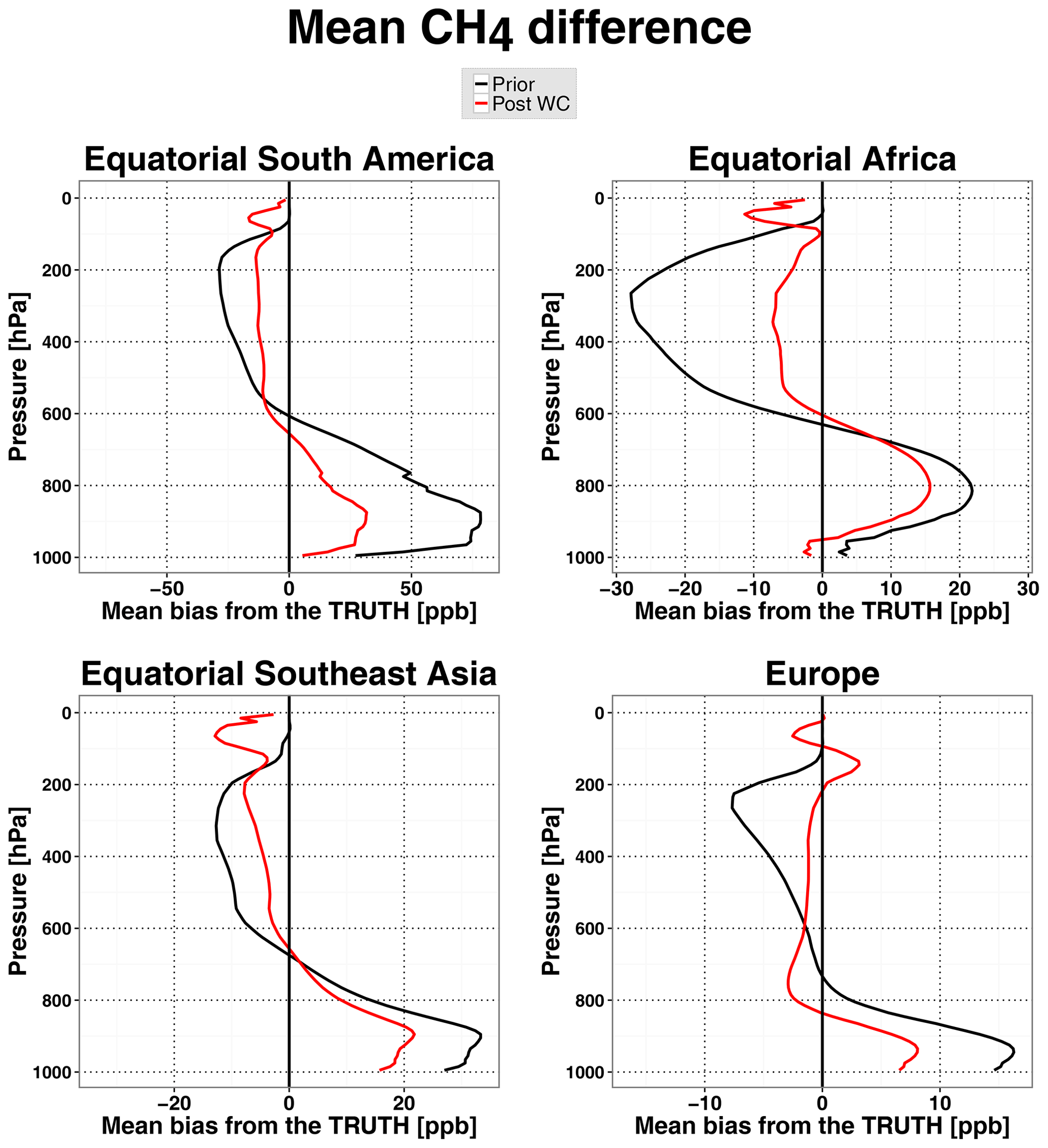
Figure 2Mean vertical profiles of the CH4 differences in March 2010 in the OSSE with biased convection for the four regions depicted in Fig. 1. The differences are between (black lines) the a priori and the true CH4 state and between (red lines) the WC optimized state and the true CH4 state.

Figure 3Mean differences in the CH4 distribution in March 2010 in the OSSE with biased chemistry. (a, d, g) Mean differences between the a priori CH4 state and the true CH4 state. (b, e, h) Mean differences between the WC optimized CH4 state and the true CH4 state. (c, f, i) The mean WC state corrections (the forcing terms) in parts per billion (ppb). Shown are the latitude–longitude differences at (a–c) the surface and (d–f) at 300 hPa, as well as the altitude–longitude differences (g–i) along the Equator. The black boxes indicate the four domains considered for the regional analysis discussed in the text and shown in Fig. 4.
The second OSSE, in which a chemistry bias was created by turning off the reaction of CH4 with OH, was the least challenging bias for the WC 4D-Var scheme to mitigate. This bias was rather smooth in the troposphere and did not contain small-scale features. Although the actual chemistry bias in the model may have a more complex vertical structure, we do not expect chemical biases to be as strongly localized as the biases associated with emissions and vertical transport. The a priori and a posteriori residual biases, as well as WC forcing terms, are shown in Fig. 3. The WC state optimization performed best over land where the a priori biases were almost completely removed. The optimization was least successful over the oceans in the lower troposphere. This situation is consistent with the fact that the assimilation of GOSAT data has lower sensitivity to variations in CH4 in the lower troposphere compared to the upper troposphere, due in part to the absence of GOSAT observations over oceans in our analysis as well as to different transport patterns and stronger winds in the upper troposphere. Shown in Fig. 4 are the mean vertical profiles of the prior and posterior bias over the same four regions considered in Fig. 2. The model does indeed successfully mitigate the bias. Over the convection regions in the tropics, there are some compensatory corrections in the lower troposphere and in the upper troposphere and lower stratosphere (UTLS), which is probably due to the fast vertical transport in these regions and the limited vertical information in the GOSAT retrievals.
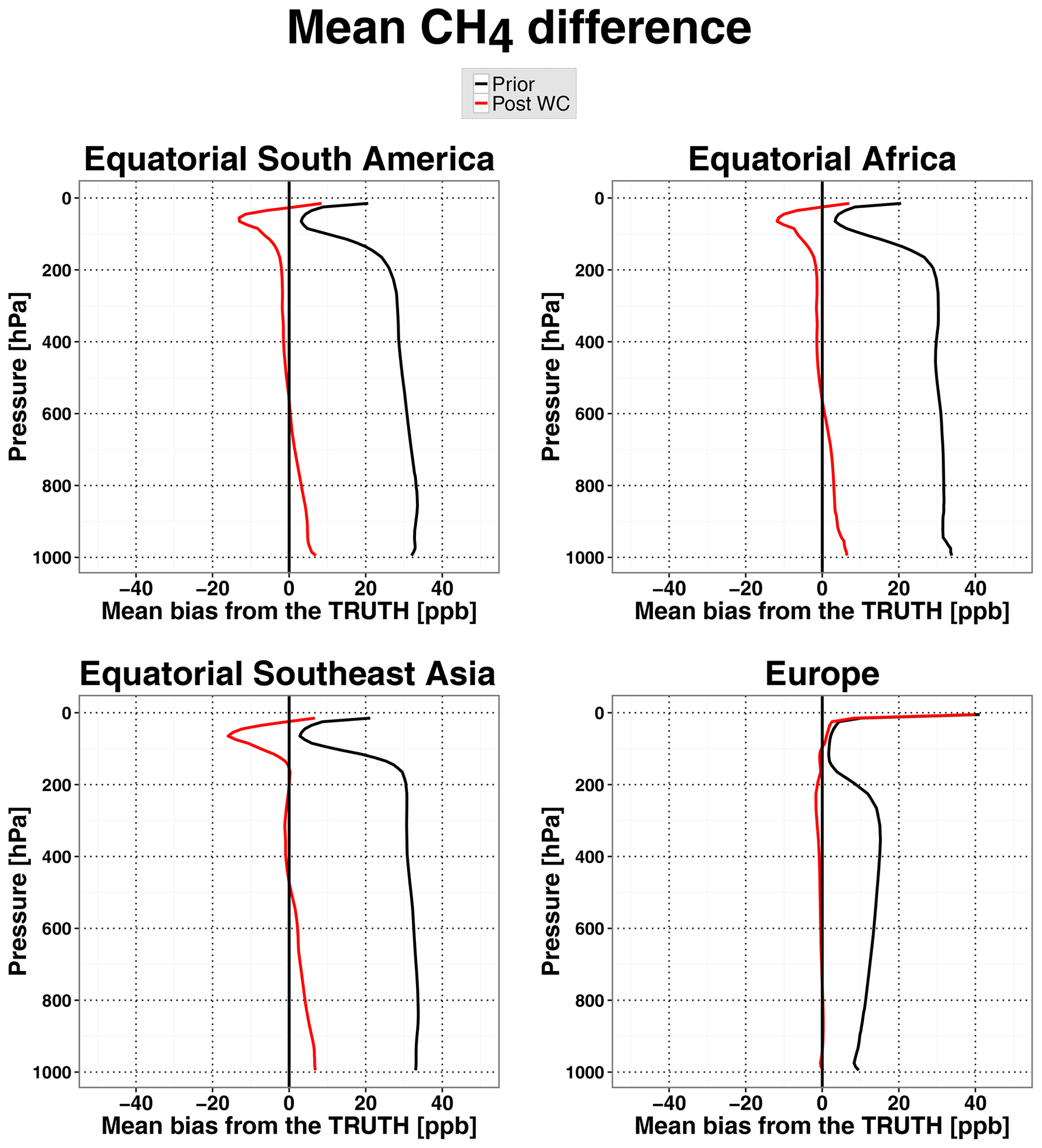
Figure 4Mean vertical profiles of the CH4 differences in March 2010 in the OSSE with biased chemistry for the four regions depicted in Fig. 3. The differences are between (black lines) the a priori and the true CH4 state and between (red lines) the WC optimized state and the true CH4 state.
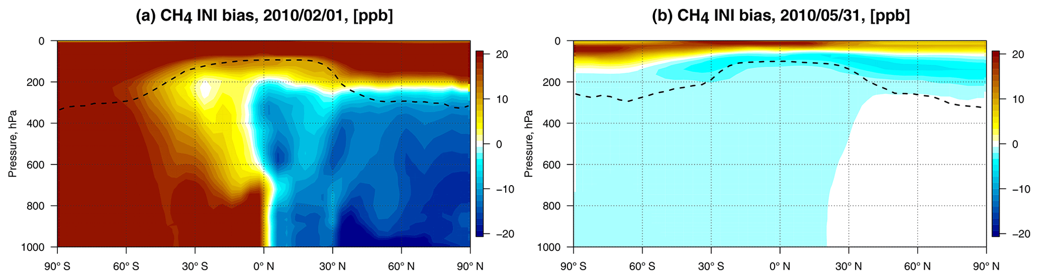
Figure 5Results of the OSSE with biased initial conditions. (a) A priori bias in initial conditions. (b) A posteriori bias at the end of the assimilation window. The dashed line represents the mean tropopause height on 31 May 2010 taken from GEOS-5 meteorological fields.
In the third OSSE, with biased initial conditions, the initial condition bias is shown in the left panel in Fig. 5. The stratosphere and southern troposphere were positively biased, whereas the northern troposphere was negatively biased. The right panel shows the structure of the a posteriori bias after the WC assimilation on the last day of the assimilation window, 31 May. It shows that the CH4 state converged to the true concentrations everywhere except in the upper stratosphere; the positive upper-stratospheric bias was compensated for in the column by a small negative CH4 bias in the troposphere and the lower stratosphere. Examination of the evolution of the initial condition bias (not shown) indicates that different regions of the atmosphere converged to the true CH4 mass at different rates, with levels above 200 hPa converging the slowest, such that by the third month the CH4 mass had not fully recovered at these levels.
3.2 Assimilation of real GOSAT retrievals
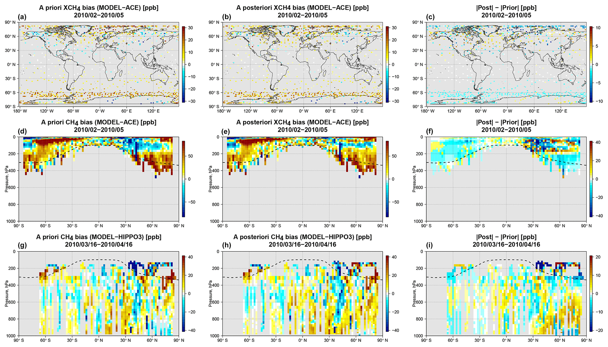
The bias between the GOSAT data and the 4∘ × 5∘ a priori and a posteriori model is shown in Fig. 6. Here we will refer to the a posteriori results as the WC_4x5 assimilation, which is our standard WC 4D-Var assimilation at 4∘ × 5∘ resolution with a 3 d forcing time window and a forcing mask G comprising the entire vertical extent of the atmosphere. As can be seen, there are large positive a priori biases at high latitudes in the Northern Hemisphere and in some low-latitude regions, such as equatorial Africa and eastern China. The WC_4x5 assimilation successfully reduces the a priori bias. There is some residual high-latitude bias, which resembles noise or bias in the GOSAT observations. In a companion analysis (Stanevich et al., 2020) in which we examine the impact of model resolution on the modeled CH4 distribution, we showed that the large positive a priori CH4 bias over China may partly be explained by weakening of the vertical transport in the model due to the coarse 4∘ × 5∘ resolution. In Stanevich et al. (2020), we also showed that a significant fraction of the high-latitude bias comes from the stratosphere and is a consequence of running the model at 4∘ × 5∘ resolution. As a result, here we repeated the GOSAT WC assimilation at the higher resolution of 2∘ × 2.5∘. The results, which are shown in Fig. 7, reveal that the high-latitude a priori bias is indeed smaller in the 2∘ × 2.5∘ model. At the higher resolution, the WC assimilation also successfully reduces the model bias. For comparison, we repeated the assimilation at 4∘ × 5∘ but optimized the emissions instead of the CH4 state. The results for this experiment, referred to as SC_4x5, are shown in Fig. 8. As can be seen, the SC assimilation leaves significantly larger residual biases. The pattern of the residual bias indicates that there were other biases that the assimilation could not fit at the expense of the emissions. We will investigate possible sources for these biases in the sections below.
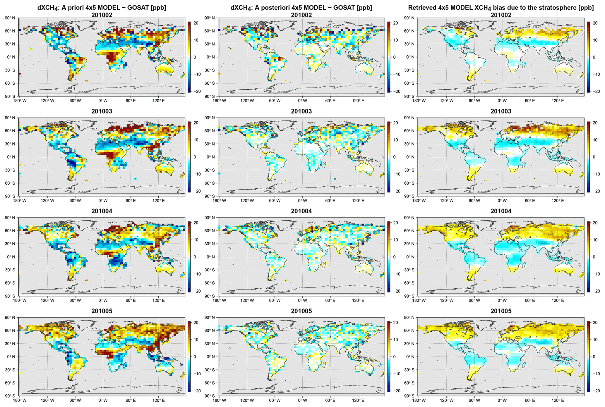
Figure 6Monthly mean fields from the 4∘ × 5∘ resolution model for February–May 2010. First column: differences between the GEOS-Chem a priori XCH4 state and the GOSAT data. Middle column: differences between the a posteriori WC_4x5 XCH4 state and the GOSAT data. Right column: the optimized stratospheric XCH4 bias correction calculated as the difference between the model simulation with optimized forcing corrections everywhere and the model simulation with the forcing corrections estimated only in the troposphere. The rows represent results for (top row) February, (second row) March, (third row) April, and (bottom row) May 2010. All model simulations were sampled at the locations and times of the GOSAT observations and smoothed with the GOSAT averaging kernels.

Figure 7Same as Fig. 6 but for the 2∘ × 2.5∘ resolution model.
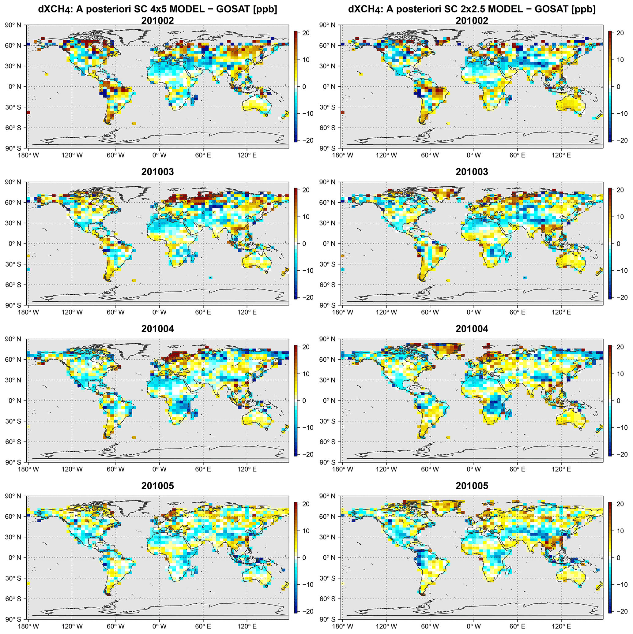
Figure 8Monthly mean differences between the GEOS-Chem a posteriori XCH4 state and GOSAT. Left column: differences between the a posteriori state from the SC flux assimilation at 4∘ × 5∘ (SC_4x5) and GOSAT. Right column: differences between the a posteriori state from the SC flux assimilation at 2∘ × 2.5∘ (SC_2x25) and GOSAT. The rows represent results for (top row) February, (second row) March, (third row) April, and (bottom row) May 2010.
The signal of surface emissions is mixed with possible model errors in the troposphere, such as those related to vertical transport. Biases in the CH4 fields caused by incorrect surface emissions will in some cases have an identical structure as those caused by biased vertical transport, which may complicate the interpretation of WC 4D-Var state corrections in the troposphere. On the other hand, it takes much longer for the surface emission signal to mix into the stratosphere. We therefore assumed that, on the short (4-month) timescale of the simulation, optimized forcing corrections ui in the stratosphere can be considered independent from the influence of surface emissions. The third column in Figs. 6 and 7 shows the actual mean monthly bias in the a priori CH4 fields that was corrected by the stratospheric forcing terms. The bias corrections in the 2∘ × 2.5∘ CH4 simulation are smaller than for the 4∘ × 5∘ simulation, which is consistent with Stanevich et al. (2020), who suggested that part of the stratospheric bias at 4∘ × 5∘ resolution is due to the model resolution itself. The WC inversion results suggest that the 4∘ × 5∘ model is positively biased in the stratosphere at high latitudes and weakly negatively biased in the tropics. In contrast, the 2∘ × 2.5∘ model is mainly negatively biased in the stratosphere, particularly around 30–40∘ N, except for a few high-latitude regions, possibly related to the polar vortex.
3.2.1 Evaluation with TCCON and NOAA data
Table 1 presents the results of the evaluation of the SC_4x5 and WC_4x5 assimilation with the in situ and TCCON data, whereas Table 2 gives the comparison results at individual TCCON sites. Based on the OSSE results in Sect. 3.1 and provided that the only model bias is due to incorrect surface emissions, we would anticipate the WC assimilation to produce generally worse fits to the surface measurements than the SC assimilation. The comparisons show that both approaches produced similar improvements in the fit to the NOAA in situ observations, with slightly better performance from the WC method. The WC assimilation had a significant impact on the overall fit to the TCCON XCH4 retrievals, whereas the SC assimilation had a much more limited impact. Table 2 shows the benefits of using the WC method at the individual TCCON sites. With the exception of Park Falls and Lamont, the WC assimilation significantly improved the correlation and reduced the bias between the model and the TCCON observations. The results suggest that the GEOS-Chem a priori CH4 simulation suffered from biases that were not only related to incorrect surface emissions.
Table 1Evaluation of a priori, SC_4x5, and WC_4x5 optimized CH4 fields using TCCON XCH4 from the stations listed in Table 2 and NOAA surface in situ observation (mean statistics for the period of February–May 2010). The first, second, and third columns represent the mean difference, standard deviation, and correlation between the model and measurements, respectively. The fourth column represents the slope of the regression line, with modeled data on the y axis and measurements on the x axis.
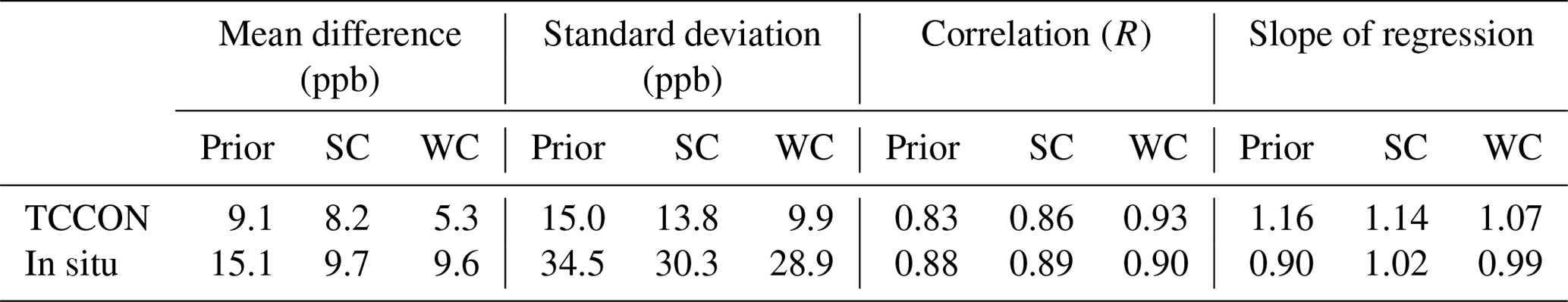
Table 2Evaluation of a priori, SC_4x5, and WC_4x5 optimized CH4 fields using TCCON XCH4 (mean station-wise statistics for the period of February–May 2010). The first, second, and third columns represent the mean difference, standard deviation, and correlation between the model and measurements, respectively.
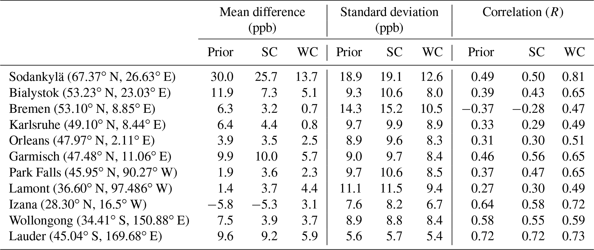
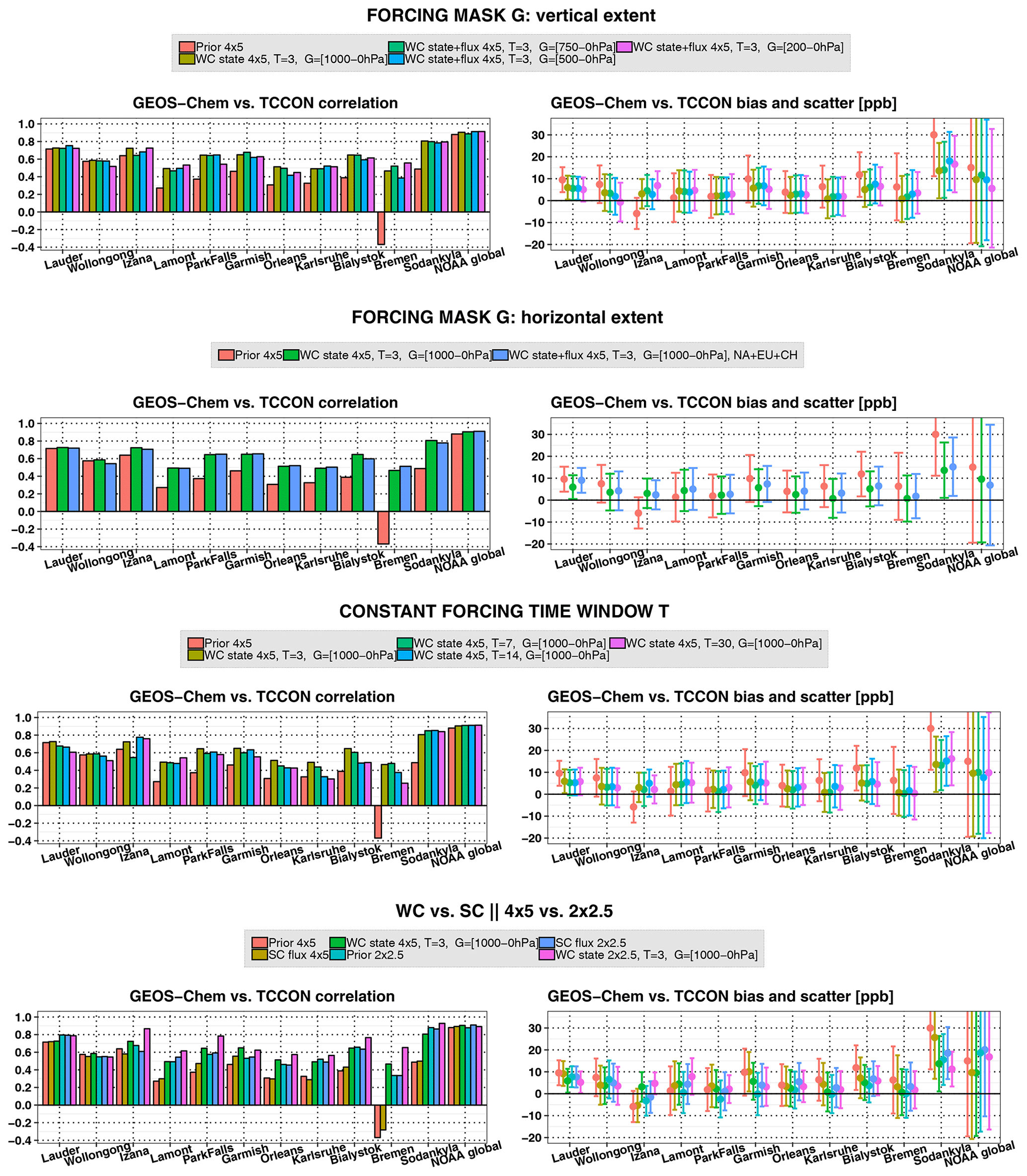
Figure 9Evaluation of the mean (February–May 2010) a priori and optimized CH4 fields using TCCON XCH4 and NOAA surface in situ observations. Results are shown for the four experiments described in Sect. 2.5. For each set of experiments (each row), the left column shows the correlation with respect to the TCCON and NOAA data, whereas the right column shows the mean bias and scatter. Top row: comparison of (red) the a priori fields, (light green) the standard WC assimilation, and the WC assimilation with the forcing terms estimated at altitudes above (dark green) 750 hPa, (blue) 500 hPa, and (purple) 200 hPa. Second row: comparison of (red) the a priori fields, (dark green) the standard WC assimilation, and (blue) the WC assimilation with joint estimation of the state and surface emissions with forcing terms estimated only over North America, Europe, and Asia. Third row: comparison of (red) the a priori fields, (light green) the standard WC assimilation, and the WC assimilation with a constant forcing window of (dark green) 7 d, (blue) 14 d, and (purple) 30 d. Bottom row: comparison of the a priori fields at (red) 4∘ × 5∘ and (light blue) 2∘ × 2.5∘, the SC assimilation at (light green) 4∘ × 5∘ and (dark blue) 2∘ × 2.5∘, and the WC assimilation at (dark green) 4∘ × 5∘ and (purple) 2∘ × 2.5∘.
The evaluation of the WC sensitivity experiments is summarized in Fig. 9. The series of WC experiments described in Sect. 2.5 were organized into four groups. The most sensitive indicator of the quality of the model–observation fit is the correlation. The scatter was close to the level of the GOSAT measurement noise and did not change much among the different assimilation experiments. In the set of experiments (first panel in Fig. 9) in which we changed the vertical extent of the forcing mask G, we found that restricting the optimized forcing to the stratosphere (altitudes above 200 hPa) resulted in correlation statistics that were only slightly worse than when we optimized the forcing throughout the whole atmosphere. This suggests that a significant part of model errors above all TCCON stations may be related to the representation of the stratosphere in the model. In addition, the bias and scatter plots show that optimization of forcing terms above 200 hPa produced the best fit to NOAA surface observations. In the experiments (second panel in Fig. 9) in which we modified the horizontal extent of the forcing mask G, we found that optimization of the forcing throughout the stratosphere and only over North America, Europe, China, and equatorial Africa in the troposphere, as described in Sect. 2.5, produced almost identical fits to the case of the full state assimilation. These four regions are major sources of CH4, and our results suggest that at the TCCON sites the model was likely affected by errors in emissions and the transport of the emission signal over these regions. Henceforth, we refer to these assimilation results as WC_4REG_4x5. In the experiments (see the third panel in Fig. 9) in which we varied the length of the forcing window from 3 to 7, 14, and 30 d, we found that the agreement at some of the stations, such as Lamont, Park Falls, and Sodankylä, was generally insensitive to increasing the length of the forcing window, which could suggest that the model above these stations was affected by slowly varying biases. The model fit at other stations, particularly Bialystok, Bremen, and Karlsruhe, degraded when the window length was increased. The latter three stations are located close to each other and are probably affected by similar model errors on synoptic timescales of about 1 week.
In the last group of experiments (see the fourth panel in Fig. 9), we compared the performance of the two 4D-Var assimilation modeling approaches (WC full state assimilation and SC flux assimilation) at the two model resolutions (4∘ × 5∘ and 2∘ × 2.5∘). The comparison suggested that, in the absence of a priori bias correction, the SC method brings limited improvements to the a prior CH4 fields at both resolutions. Indeed, we conclude that the SC assimilation at the 4∘ × 5∘ resolution is futile as the a priori model at 2∘ × 2.5∘ resolution produces a better fit to the TCCON observations than the SC 4∘ × 5∘ assimilation. The performance of the SC assimilation at the 2∘ × 2.5∘ resolution was similar to but was surpassed by the “best-fit” WC state assimilation at the 4∘ × 5∘ resolution in term of its fit to TCCON and NOAA in situ measurements. Overall, the WC state assimilation at 2∘ × 2.5∘ resolution generated the best model fit to TCCON observations. However, in all 2∘ × 2.5∘ resolution experiments the model bias against NOAA surface measurements was larger compared to the 4∘ × 5∘ experiments. For example, the smallest WC a posteriori bias at 4∘ × 5∘ was about 10 ppb, whereas at 2∘ × 2.5∘ it was about 17 ppb.
Another important conclusion can be drawn from the fact that the WC assimilation at both model resolutions significantly improved the model fit to Izana measurements (see the fourth panel in Fig. 9). The Izana station is located at an altitude of 2370 m above sea level on a small island near the coast of Africa that has no local CH4 emission sources. The model at 2∘ × 2.5∘ and 4∘ × 5∘ resolutions is not able to resolve the topography of the island. Therefore, the model transport in the vicinity of this high-altitude station, particularly in the lower troposphere, may be subject to similar errors at both the 2∘ × 2.5∘ and 4∘ × 5∘ resolutions. Hence, the improvement in the assimilated CH4 fields may be related to the corrected model errors in the upper troposphere and the stratosphere rather than in the lower troposphere where topography-related errors would be dominant.
The WC full state assimilation at 4∘ × 5∘ leaves weak positive biases in the GEOS-Chem fields against the TCCON observations (excluding Sodankylä) in most of the experiments. Mean a posteriori inter-station bias at 4∘ × 5∘ (2∘ × 2.5∘) resolution is 3.4 ppb (4.0 ppb) (excluding Sodankylä), while the scatter is 8.6 ppb (7.3 ppb) (excluding Sodankylä). It is not clear if the GOSAT data are positively biased or if this could be caused by differences between the GOSAT and TCCON averaging kernels in the stratosphere and the fact that, for example, the stratospheric model bias was not fully recovered by the assimilation, particularly during the first couple of months of the assimilation period. The results also do not indicate the presence of a latitudinal bias between TCCON and GEOS-Chem and hence between TCCON and GOSAT.
There is a larger positive XCH4 bias between the model and Sodankylä measurements of 12.6 and 11.2 ppb for the WC assimilation at 4∘ × 5∘ and 2∘ × 2.5∘ resolution, respectively; however, the correlation is also high at 0.81 and 0.93, respectively. Tukiainen et al. (2016) and Ostler et al. (2014) pointed to the fact that polar vortex conditions at high-latitude stations may induce biases in TCCON XCH4 retrievals. It has been claimed that a priori profiles in the retrievals do not account for and are not adjusted to these dynamic conditions; hence, they significantly deviate from the real CH4 profiles. When there is not enough information in the spectra to correct for such discrepancies, the XCH4 retrievals can be systematically biased. It is possible that both GOSAT and TCCON could have been affected by the polar vortex conditions during some days in February–April 2010 so that the biases in co-located retrievals are partially canceled. It should also be noted that the negative a priori correlation between the model and Bialystok XCH4 measurements is partly caused by the limited number (84) of measurements during the 4-month assimilation time window.
3.2.2 Evaluation with ACE-FTS and HIPPO-3 data
Figures and 10 show the results of the GEOS-Chem comparison with the ACE-FTS and HIPPO-3 data. Model versus ACE-FTS data are shown only in the stratosphere in order to exclude potentially biased data due to interference with clouds in the upper troposphere. The mean XCH4 difference between GEOS-Chem and ACE-FTS that is shown was obtained by artificially extending the ACE-FTS CH4 profiles down into the troposphere using the GEOS-Chem fields and then applying the GOSAT column averaging kernels. Consistent with Saad et al. (2016), the CH4 differences reveal that the a priori 4∘ × 5∘ model has a positive stratospheric bias that can be as large as 250 ppb averaged zonally (see Fig. ). The HIPPO-3 comparison also showed that the 4∘ × 5∘ model is positively biased in the stratosphere and slightly negative in the troposphere. Wang et al. (2017) showed that similar positive CH4 biases at middle and high latitudes exist in TM3, TM5, and Laboratoire de Météorologie Dynamique (LMDz) CTMs. The 4∘ × 5∘ WC assimilation reduced the positive stratospheric bias with respect to both HIPPO-3 and ACE-FTS, but it did not remove it completely. For example, the maximum model minus ACE-FTS XCH4 bias due to the stratosphere was reduced from about 40 to 30 ppb. The average negative tropospheric CH4 bias relative to HIPPO-3 was reduced. It is possible that the WC method was not able to properly localize the stratospheric bias. However, the validation analysis may also reflect the influence of the slow recovery of the stratospheric CH4 fields from the bias in the initial conditions. Therefore, discrepancies in the stratospheric CH4 field from the initial conditions in the first 2 months of the WC assimilation could be contributing to the observed HIPPO-3 and ACE-FTS bias. Unfortunately, the measurements are either too sparse or limited in space and time to verify this assumption.

Figure 10Evaluation of the mean (February–May 2010) a priori and WC_4x5 optimized CH4 fields using ACE-FTS and HIPPO-3 CH4 measurements. Shown are (a, d, g) the a priori bias, (b, e, h) the a posteriori bias, and (c, f, i) the reduction in absolute bias. (a–c) XCH4 bias between GEOS-Chem and ACE-FTS. (d–f) Zonally averaged CH4 bias between GEOS-Chem and ACE-FTS. (g–i) CH4 bias between GEOS-Chem and HIPPO-3. We used ACE-FTS retrievals only in the stratosphere. The XCH4 bias between GEOS-Chem and ACE-FTS was obtained by augmenting the ACE-FTS profile in the stratosphere with the GEOS-Chem profile in the troposphere and smoothing the vertical CH4 profile with mean meridional GOSAT averaging kernels. The dashed line represents the mean tropopause height.
The positive a priori stratospheric bias relative to ACE-FTS and HIPPO-3 was significantly smaller at 2∘ × 2.5∘ than at the 4∘ × 5∘ resolution (see Fig. 10); however, it was not completely removed. Stratospheric CH4 fields in the Northern Hemisphere (NH) above 200 hPa even became negatively biased at 2∘ × 2.5∘, particularly around 30–40∘ N, where the absolute bias became larger than at 4∘ × 5∘. The WC assimilation at 2∘ × 2.5∘ further corrected the positive biases and significantly reduced the negative bias around 30–40∘ N. As can be inferred from Fig. 7, the latter covered the entire latitudinal band but was particularly pronounced over the Himalayas. Despite the reduction of the stratospheric bias, the 2∘ × 2.5∘ WC assimilation introduces a positive CH4 bias relative to HIPPO-3 in the NH lower troposphere.
4.1 Stratospheric bias
The sensitivity experiments carried out in Sect. 2.4 suggest that a stratospheric bias introduced in the system through the initial conditions has the slowest correction rate. However, by the start of the last month of the assimilation, May 2010, the bias is either removed or does not change much with time. Therefore, we focus the discussion here on the stratosphere in the month of May 2010, with the assumption that the model is free of the influence of the initial conditions. Figure 11 compares the a priori CH4 fields to the optimized fields from the WC_4x5 and SC_4x5 assimilations. The top panel shows that corrections in the stratospheric CH4 abundance are the most pronounced feature of the WC optimized CH4 fields and that changes are smaller in the zonal mean tropospheric fields. The bottom panel is presented to contrast the behavior of the two 4D-Var approaches. It shows that the SC assimilation attempts to correct the positive high-latitude stratospheric CH4 bias at the expense of surface emissions. This results in a negative CH4 bias in the lower troposphere, while the surface signal hardly impacts the stratosphere. In the WC assimilation, stratospheric CH4 was significantly reduced at high latitudes and increased in the tropics relative to the a priori, which is consistent with the correction of the biases shown in Figs. and 10. The changes are more substantial in the Northern Hemisphere due to the asymmetrically larger number of GOSAT measurements in the Northern Hemisphere since we are assimilating data only over land.

Figure 12Zonal mean CH4 differences (in ppb) in May 2010 between (a) the WC_4x5 optimized state and the a priori fields and (b) between the SC_4x5 optimized state and the a priori fields. The dashed line represents the mean monthly tropopause height.
Large biases in the stratosphere were previously identified in GEOS-Chem (Saad et al., 2016) and in other chemistry transport models (Strahan and Polansky, 2006; Patra et al., 2011; Ostler et al., 2016). The problem was mainly linked to biases in the meridional Brewer–Dobson circulation in the stratosphere and in the rate of troposphere–stratosphere exchange. However, neither mechanism was analyzed in detail. Indeed, the observed changes in Fig. 11 may partly reflect discrepancies in the Brewer–Dobson circulation projected from the initial conditions. In particular, meridional overturning that is too rapid in the months prior to the assimilation would have transported excess CH4 from the tropics and to the high latitudes. In the companion study, Stanevich et al. (2020) show that the stratospheric bias in GEOS-Chem can also be due to increased numerical diffusion at the coarse horizontal model resolution. This leads to additional unphysical horizontal mixing between the troposphere and the stratosphere and between the high latitudes and the tropics in the stratosphere.
4.2 Tropospheric bias
4.2.1 Pattern of forcing terms
The forcing terms are corrections applied to the CH4 fields at each model time step. This time step is 30 and 15 min for the 4∘ × 5∘ and 2∘ × 2.5∘ simulations, respectively. In order to compare the forcing terms in the two simulations, we added together the state corrections at two successive 2∘ × 2.5∘ time steps. Therefore, all forcing terms discussed in this section are presented for 30 min time intervals. The first column in Fig. 12 presents forcing terms in the troposphere optimized by the WC_4x5 assimilation. The observed structure of the forcing terms simultaneously mitigated model errors from multiple sources. In this section, we attempt to give the most likely explanation for the retrieved pattern of the state correction and identify sources of regional biases.
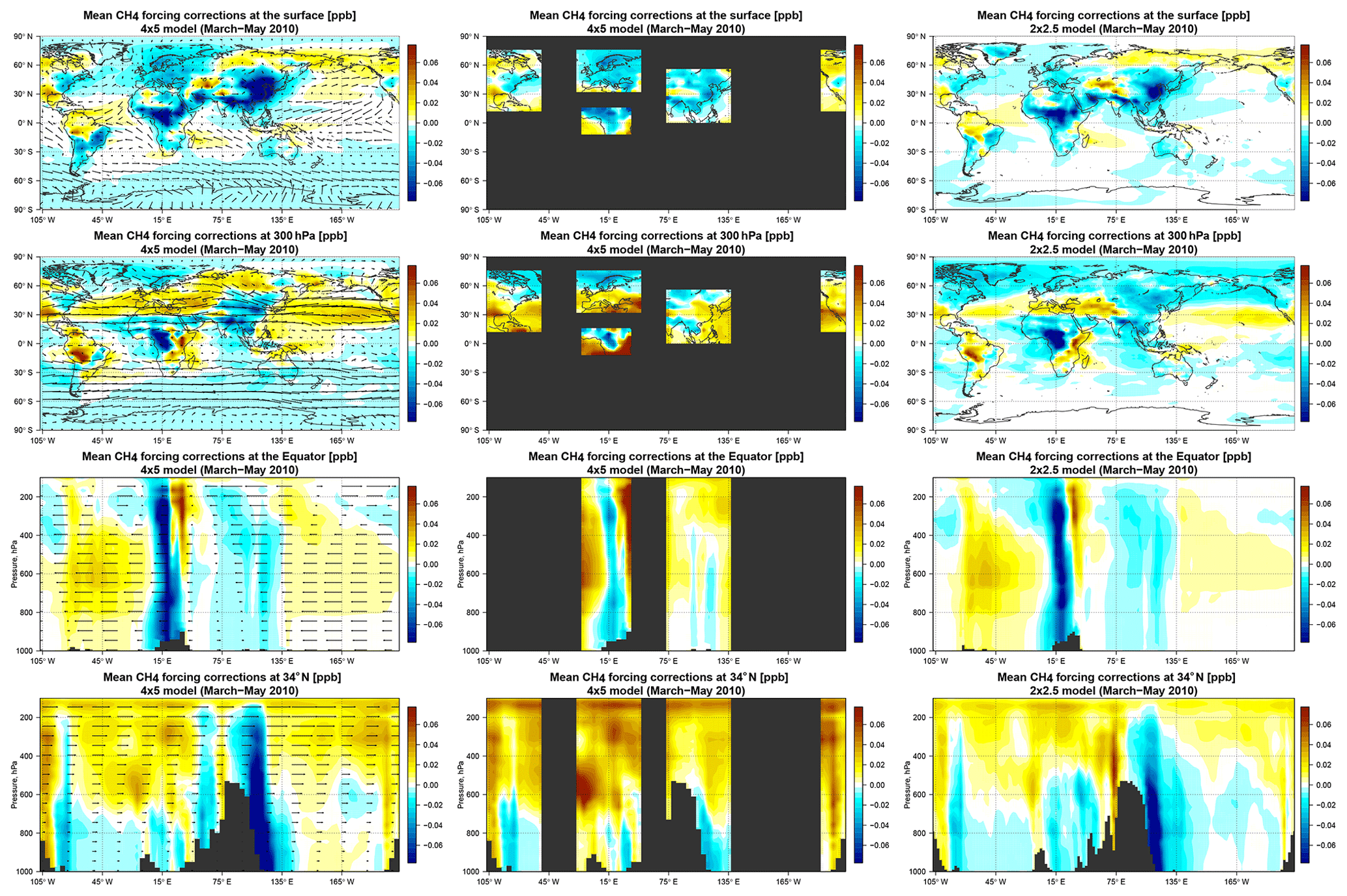
Figure 13Mean optimized forcing terms (in ppb) for March–May 2010. Left column: WC_4x5 assimilation at 4∘ × 5∘. Middle column: WC_4REG_4x5 assimilation at 4∘ × 5∘. Right column: WC_2x25 inversion at 2∘ × 2.5∘. Top row: forcing terms at the surface. Second row: forcing terms at 300 hPa. Third row: altitude–longitude distribution of the forcing terms along the Equator. Bottom row: altitude–longitude distribution of the forcing terms along 34∘ N. In the plots in the left column, arrows represent the direction and relative magnitude of horizontal winds.
In general, the original a priori CH4 fields can be affected by model errors that either occurred during the assimilation period or were projected onto the assimilation window from the initial conditions. Here, we investigate the former case. Given the results of the OSSE with biased initial conditions in Sect. 3.1, we focus in Fig. 12 on the mean forcing terms in the last 3 months of the assimilation (March–May 2010) as they are much more likely to be related to recent model errors than to biases in the initial conditions. The temporally averaged structure also gives insight into systematic model errors and is easier to interpret. Figure 12 (first column) shows that negative forcing terms dominate near the surface and in the lower troposphere, particularly over Europe, equatorial Africa, and East Asia. The CH4 reduction at the surface is consistent with NOAA observations. Positive state corrections are more frequently found in the upper troposphere, mainly at midlatitudes over the Pacific and Atlantic oceans as well as over Europe and a significant part of Russia. There are also several regions, such as eastern China and equatorial Africa, where the forcing terms are negative throughout the entire tropospheric column. Vertical slices over midlatitudes (bottom right panel) show that strong negative corrections over the east coast of Asia and North America are accompanied by positive corrections in the upper troposphere downwind of the continents. Forcing terms are generally weaker in the lower troposphere over the oceans where we lack GOSAT observations.
Generally, corrections of one sign with monotonically decaying magnitude from the surface to the upper troposphere could be associated with biases in the surface emissions, while the dipole structures with corrections of the opposite sign in the upper and lower troposphere could be related to errors in vertical transport. However, it is not feasible to uniquely identify the origin of model errors from the pattern of forcing terms because model errors from separate sources are mixed in the atmosphere and the estimation of the forcing terms is an under-constrained inverse problem.
Still, we may try to identify possible sources of model errors. For example, initial assessment of the state corrections pointed to potential issues in vertical transport. Indeed, the dipole structure of the forcing terms could indicate that upward transport of CH4 at midlatitudes may be insufficient, particularly over regions with strong vertical CH4 gradients that are present over large sources of CH4. At NH midlatitudes the major CH4 source regions are China, the US, and Europe. Moreover, the eastern parts of China and North America are located in regions of significant extratropical cyclone activity (Stohl, 2001; Shaw et al., 2016), where CH4 emitted from the surface is being lifted into the free troposphere in warm conveyor belts associated with these cyclones (Kowol-Santen et al., 2001; Li et al., 2005; Sinclair et al., 2008; Lin et al., 2010). Moist convection over land could also contribute to the total transport bias; however, convective transport is not strong over these midlatitude regions during the months of February–May.
A similar vertical structure in the forcing terms was identified above and downwind of eastern North America and China (see the first column, fourth row of Fig. 12). The WC method applied negative corrections over land from the surface to the upper troposphere, large positive corrections in the upper troposphere, and weakly negative corrections in the lower troposphere over the oceans downwind of the continents. The WC method may suggest that vertical transport over eastern parts of the continents has to be stronger. In such a case, more CH4 emitted from local sources reaches the middle to upper troposphere and is transported away from the continents by strong westerly winds. Meanwhile, CH4 concentrations in the entire atmospheric column over land and in the lower troposphere over the adjacent oceans are reduced. Therefore, the large positive a priori bias between the model and GOSAT over China shown in Fig. 6 (first column) may be partly attributed to weak local uplift of CH4.
Another region of interest, as suggested by the WC assimilation (Fig. 12, first column, third row), is equatorial Africa. Similar to China, a large positive a priori model XCH4 bias was found here. However, due to the observational coverage, there are limited direct constraints on the CH4 outflow from equatorial Africa except for sparse GOSAT observations over South America. While the African XCH4 bias could be related to positively biased local a priori surface emissions, the WC assimilation also suggested another transport-related explanation. The WC assimilation applied negative CH4 forcing terms over central Africa and positive forcing terms downwind in the middle troposphere (between 400 and 800 hPa) over the Atlantic Ocean. Such a pattern of state correction could point to potential errors in CH4 outflow from the African continent. Southern Africa is characterized by a persistent high-pressure system that drives easterly outflow from southern tropical Africa to the Atlantic in the lower to middle troposphere (Garstang et al., 1996). In their analysis of the sources of moisture in the Congo Basin, Dyer et al. (2017) showed that there is a strong export of moisture from southern tropical Africa to the Atlantic between 800 and 500 hPa. Furthermore, Arellano et al. (2006) found, in their inversion analysis of carbon monoxide (CO) data from the MOPITT instrument, a discrepancy between their a posteriori CO and observations at Ascension Island, which they speculated could be due to errors in the altitude dependence of the outflow from Africa in the GEOS-Chem model. It is possible that too much CH4 is being convectively lifted to the upper troposphere over central Africa and not enough is exported out over the Atlantic in the lower troposphere. Figure 1 (first column) displays the bias in CH4 fields when convection was turned off in the model. This caused CH4 emitted over Africa to take a different transport pathway. Instead of being lifted up over the continent, more CH4 was transported out to the Atlantic in the lower to middle troposphere between 500 and 900 hPa. Under such conditions, CH4 is simultaneously depleted over the continent and increased over the Atlantic, which is similar to what the WC forcing terms suggest. We cannot determine the exact origin of the XCH4 bias over Africa, but the forcing terms do suggest the presence of a transport bias.
The estimation of the forcing terms is an under-constrained inverse problem. Consequently, here we evaluate the impact of reducing the dimensionality of the inverse problem by limiting the region of the atmosphere where the forcing terms should be applied. This was done in the WC_4REG_4x5 assimilation, in which we restricted the forcing optimization to the stratosphere and only over the main CH4 anthropogenic emission regions in the troposphere. The results presented in Sect. 3.2.1 suggest that the WC_4x5 and WC_4REG_4x5 assimilations produced similar fits to the independent observations. Therefore, errors affecting the model, at least at the location of the validation stations, could emerge from the NA, CH, EU, EQAf, or STRAT regions. The second column in Fig. 12 presents the structure of optimized forcing terms from the WC_4REG_4x5 assimilation in which the number of optimized variables was reduced using the forcing mask G. Over China and North America, the forcing terms acquired a better-defined dipole structure with a positive correction in the upper troposphere and a negative correction in the lower troposphere. Over equatorial Africa, the region of positive corrections in the mid-troposphere moved closer to the continent.
4.2.2 Dependence of the forcing terms on model resolution
Coarsening the model resolution from 2∘ × 2.5∘ to 4∘ × 5∘ can be considered equivalent to introducing errors in the finer-resolution model. Yu et al. (2018) and Stanevich et al. (2020) showed that at coarse resolution vertical transport in GEOS-Chem is weakened due to loss of eddy mass flux and air mass flux in the regridding of the meteorological fields. Stanevich et al. (2020) also showed that the efficiency of transport barriers is reduced due to increased numerical diffusion, which causes unphysical mixing between the interior and the exterior of the polar vortex, mixing of CH4 between the tropical and extratropical branch of the Brewer–Dobson circulation that is too rapid, and increased troposphere–stratosphere exchange. Thus, in Fig. 12 we compare the forcing terms from the 4∘ × 5∘ assimilation (WC_4x5) with those from the 2∘ × 2.5∘ WC assimilation (WC_2x25). Differences between the 2∘ × 2.5∘ and 4∘ × 5∘ forcing represent the response of the WC method to the resolution-induced transport errors. We found that the magnitude of the negative forcing term was reduced in the lower troposphere, particularly over China. Similarly, the magnitude of positive forcing terms was reduced in the upper troposphere. The pattern of forcing terms on the vertical slice at midlatitudes became significantly weaker. Comparison of Figs. 6 and 7 also suggests smaller stratospheric corrections at the 2∘ × 2.5∘ resolution. At the same time, the structure and magnitude of forcing terms at the Equator (particularly over equatorial Africa) were not significantly affected by the increase in resolution.
Several conclusions follow from Fig. 12. First, the results suggest that a large fraction of model errors at 4∘ × 5∘ resolution, particularly in the stratosphere and over midlatitudes in the troposphere, are resolution-induced. Second, although the magnitude of the forcing terms at the 2∘ × 2.5∘ resolution is smaller, the pattern remains similar, which implies that the 2∘ × 2.5∘ resolution model may still be affected by the same type of transport errors. Third, the assumptions made about sources of model errors in the tropics, particularly over equatorial Africa, still apply to the 2∘ × 2.5∘ simulation as the structure and magnitude of forcing terms remained unresponsive to the model resolution. It is possible that these regions are dominated by discrepancies in moist convective transport that are large at 2∘ × 2.5∘ and 4∘ × 5∘.
In this study, we assessed errors in the global GEOS-Chem chemistry transport model during the 4-month period of February–May 2010 using the weak-constraint 4D-Var data assimilation method at model resolutions of 4∘ × 5∘ and 2∘ × 2.5∘. This was done by constraining simulated CH4 fields with GOSAT XCH4 retrievals. This represents the first application of the WC 4D-Var scheme for assimilation of GOSAT XCH4 retrievals to characterize model errors in a CTM.
An analysis of the sensitivity of the GOSAT measurements to the atmospheric CH4 state found that the XCH4 retrievals are most sensitive to CH4 mass changes in the stratosphere and in the upper troposphere in the Northern Hemisphere, which was explained by the GOSAT observational coverage and stronger horizontal winds in the UTLS, allowing the CH4 perturbations to be observed by a larger number of measurements. Sensitivity at the Equator was about half that at northern midlatitudes. In a series of OSSEs, the observations and the WC method were tested to determine the ability of the system to recover “unknown” errors in CH4 fields associated with artificially introduced biases in convection, chemistry, and initial conditions. We found that when not supplied with any information about the errors, the WC method was able to significantly mitigate biases in the CH4 fields with slowly changing spatial structures, but it was not able to correct strongly localized biases, particularly those in the boundary layer. Despite having almost flat averaging kernels in the troposphere, our analysis showed that the GOSAT XCH4 retrievals could help constrain the vertical distribution of model errors when convection was turned off in the model. The WC method needed about a month to recover the bias introduced in the initial condition in the troposphere and about 2 months to do so in the stratosphere. Generally, the method was successful in mitigating model errors of unknown origin and magnitude. However, more optimal performance could be achieved by supplying the method with additional information about model errors, such as their temporal and spatial correlation, using the model error covariance matrix Q. However, characterizing these correlations will be challenging.
The WC method was tuned in a set of experiments to diagnose real model errors in the GEOS-Chem CTM at the 4∘ × 5∘ resolution. The a posteriori model fit to independent observations, such as ACE-FTS, HIPPO-3, TCCON, and NOAA surface measurements, was used to evaluate the assimilation. Initial comparisons suggested that GEOS-Chem was affected by biases not solely related to discrepancies in surface emissions. Results suggested that the modeled CH4 fields at the location of most NH TCCON stations were affected by slowly varying biases. However, a few stations, such as Bialystok, Bremen, and Karlsruhe, were more likely influenced by errors varying on timescales of 1 week. The evaluations pointed to a large positive bias in the stratosphere relative to ACE-FTS and HIPPO-3 measurements and a weakly negative bias in the middle to upper troposphere relative to HIPPO-3 data. The WC assimilation was able to mitigate the negative tropospheric bias and partly removed the stratosphere bias. We found that the SC 4D-Var assimilation that optimized the surface emissions had only a limited impact on the model fits. Furthermore, the WC assimilation at 4∘ × 5∘ resolution performed better than the SC assimilation at 2∘ × 2.5∘ resolution. Meanwhile, the results showed that running the a priori model at 2∘ × 2.5∘ resolution produced better agreement with TCCON observations than the a posteriori fields from the SC 4D-Var surface emission optimization at 4∘ × 5∘.
State corrections at the 4∘ × 5∘ resolution also explicitly pointed to issues with vertical transport, suggesting that vertical transport of CH4 at midlatitudes over the large CH4 source regions of eastern China and North America is too weak. In the tropics, the WC inversion corrected for large positive XCH4 biases over equatorial Africa. From the pattern of forcing terms, it remained unclear whether the bias over Africa was related to surface emissions. However, the WC method suggested the possibility of biased CH4 outflow from the African continent to the Atlantic Ocean in the mid-troposphere, which could be related to a discrepancy in the partitioning between deep convection transport to the upper troposphere and shallow outflow to the Atlantic Ocean.
In a companion analysis, Stanevich et al. (2020) examined the impact of model resolution on CH4 simulation and found larger model biases at 4∘ × 5∘ compared to 2∘ × 2.5∘. We found that assimilating the GOSAT data at the higher resolution of 2∘ × 2.5∘ produced state corrections that were similar to those obtained at 4∘ × 5∘. However, the magnitude of these corrections in the stratosphere and in the midlatitude troposphere was significantly reduced at the higher resolution. This suggests that the model at both resolutions was affected by transport errors of similar origin, although less so at the 2∘ × 2.5∘ resolution. The WC assimilation also corrected for the negative CH4 bias relative the ACE-FTS and HIPPO in the northern midlatitude stratosphere, which was found only at the 2∘ × 2.5∘ resolution, and located this bias particularly over the Himalayas. However, the origin of this bias remained unclear.
In our analysis, we used only GOSAT CH4 data over land. However, XCH4 glint measurements over oceans could help better constrain the vertical structure of the model errors. The WC 4D-Var assimilation of shorter-lived species, such as CO, could also help better diagnose model errors, especially when transport and emission errors mask each other in CH4 fields, although shorter-lived species may also be more strongly affected by errors in chemistry. The advantage of CH4 is its longer memory of model transport; however, shorter-lived gases are more strongly affected by, and hence may be more sensitive to, the same model errors. Clearly, the detected transport error at the 4∘ × 5∘ resolution would have a considerable impact on inferred emissions if the evolution of the model state were assumed to be perfect, as is the case in SC 4D-Var. Instead of reducing the positive high-latitude bias in the stratosphere, the 4∘ × 5∘ SC 4D-Var surface flux assimilation negatively biased the lower troposphere. The SC inversion also significantly reduced Chinese CH4 emissions by incorrectly attributing model errors in vertical transport to emissions. Some of the detected transport errors were significantly smaller at the 2∘ × 2.5∘ resolution, while others remained resolution-independent. The effect of these remaining errors at the 2∘ × 2.5∘ resolution has to be further investigated.
In the context of optimizing fluxes, potentially any CTM may be improved if the signal from the surface emissions can be separated from other model errors. This would be a rather challenging task for GOSAT XCH4 measurements. Further analysis is needed on this problem, particularly on the design of the model error covariance matrix Q. For example, Trémolet (2007) proposed a design based on statistics of model tendencies. The Q matrix had a rather primitive structure in our analysis, although it is sufficient for the objectives of this work. Based on our initial assessment of model errors, the structure of Q can be further improved. In the meantime, the WC 4D-Var method has a number of immediately useful applications. In general, it is a valuable instrument for diagnosing model errors. It can also be used as a tool to produce a better estimate of the CH4 state in a model in order to provide boundary and initial conditions for forecasting purposes or regional-scale analysis at higher spatial resolution.
The GOSAT satellite data are described in Parker et al. (2015) and are available from the European Space Agency Greenhouse Gases Climate Change Initiative at http://cci.esa.int/ghg (last access: 21 May 2021). The individual TCCON GGG2014 data sets used in the analysis are cited in the paper, and these references are included in the reference list. The TCCON data are available at https://tccondata.org/2014 (last access: 21 May 2021) (TCCON, 2014). The NOAA-ESRL Global Greenhouse Gas Reference Network data (Dlugokencky et al., 2016) are available at ftp://aftp.cmdl.noaa.gov/data/trace_gases/ch4/flask/surface/ (last accessed: 21 May 2021). The HIPPO aircraft data (Wofsy et al., 2011) are available at https://www.eol.ucar.edu/field_projects/hippo/ (last access: 21 May 2021). The ACE-FTS data (Waymark et al., 2013) are available at https://databace.scisat.ca/level2/ace_v3.5_v3.6/ (last access: 21 May 2021), and registration is required to download the data. The code for the GEOS-Chem model and its adjoint (Henze et al., 2007) is publicly available, and instructions for downloading the adjoint model are available at http://wiki.seas.harvard.edu/geos-chem/index.php/GEOS-Chem_Adjoint (last access: 21 May 2021). The output from the GEOS-Chem model simulations used in this analysis is available upon request.
IS led the study and wrote the paper. DBAJ and KS guided the work and edited the paper. RJP and HB provided GOSAT retrievals. DW, JN, CP, TW, RS, MS, FH, RK, NMD, and VAV provided TCCON data. KAW provided insight into the use of ACE-FTS data. DKH, MK, and FD assisted in the initial configuration of the model simulation. All co-authors read and commented on the paper.
The authors declare that they have no conflict of interest.
We thank Steven C. Wofsy for providing HIPPO aircraft data and Robert J. Parker for providing GOSAT XCH4 data. Robert J. Parker was funded via an ESA Living Planet Fellowship. Robert J. Parker and Hartmut Boesch acknowledge funding from the UK National Centre for Earth Observation (NCEO), the ESA Greenhouse Gas Climate Change Initiative (GHG-CCI), and the EU Copernicus Climate Change Service (C3S). We thank the Japanese Aerospace Exploration Agency, the National Institute for Environmental Studies, and the Ministry of Environment for the GOSAT data and their continuous support as part of the joint research agreement. This research used the ALICE High-Performance Computing Facility at the University of Leicester for the GOSAT retrievals.
This research has been supported by NSERC (grant nos. 197367-2011 and RGPIN-2019-06804), the Canadian Space Agency (grant no. 11STFATO38), and Environment and Climate Change Canada (grant no. GCXE17S037). Funding for Wollongong TCCON is provided in part by the Australian Research Council (ARC) (grant nos. DP160101598, DP140101552, DP110103118, and LE0668470). The Atmospheric Chemistry Experiment (ACE), also known as SCISAT, is a Canadian-led mission mainly supported by the Canadian Space Agency and NSERC.
This paper was edited by Patrick Jöckel and reviewed by four anonymous referees.
Alexe, M., Bergamaschi, P., Segers, A., Detmers, R., Butz, A., Hasekamp, O., Guerlet, S., Parker, R., Boesch, H., Frankenberg, C., Scheepmaker, R. A., Dlugokencky, E., Sweeney, C., Wofsy, S. C., and Kort, E. A.: Inverse modelling of CH4 emissions for 2010–2011 using different satellite retrieval products from GOSAT and SCIAMACHY, Atmos. Chem. Phys., 15, 113–133, https://doi.org/10.5194/acp-15-113-2015, 2015. a
Arellano, A. F., Kasibhatla, P. S., Giglio, L., van der Werf, G. R., Randerson, J. T., and Collatz, G. J.: Time-dependent inversion estimates of global biomass-burning CO emissions using Measurement of Pollution in the Troposphere (MOPITT) measurements, J. Geophys. Res.-Atmos., 111, D09303, https://doi.org/10.1029/2005JD006613, 2006. a
Bergamaschi, P., Frankenberg, C., Meirink, J. F., Krol, M., Villani, M. G., Houweling, S., Dentener, F., Dlugokencky, E. J., Miller, J. B., Gatti, L. V., Engel, A., and Levin, I.: Inverse modeling of global and regional CH4 emissions using SCIAMACHY satellite retrievals, J. Geophys. Res.-Atmos., 114, D22301, https://doi.org/10.1029/2009JD012287, 2009. a
Bernath, P. F., McElroy, C. T., Abrams, M. C., Boone, C. D., Butler, M., Camy-Peyret, C., Carleer, M., Clerbaux, C., Coheur, P.-F., Colin, R., DeCola, P., DeMazière, M., Drummond, J. R., Dufour, D., Evans, W. F. J., Fast, H., Fussen, D., Gilbert, K., Jennings, D. E., Llewellyn, E. J., Lowe, R. P., Mahieu, E., McConnell, J. C., McHugh, M., McLeod, S. D., Michaud, R., Midwinter, C., Nassar, R., Nichitiu, F., Nowlan, C., Rinsland, C. P., Rochon, Y. J., Rowlands, N., Semeniuk, K., Simon, P., Skelton, R., Sloan, J. J., Soucy, M.-A., Strong, K., Tremblay, P., Turnbull, D., Walker, K. A., Walkty, I., Wardle, D. A., Wehrle, V., Zander, R., and Zou, J.: Atmospheric Chemistry Experiment (ACE): Mission overview, Geophys. Res. Lett., 32, L15S01, https://doi.org/10.1029/2005GL022386, 2005. a
Blumenstock, T., Hase, F., Schneider, M., Garcia, O., and Sepulveda., E.: TCCON data from Izana, Tenerife, Spain, Release GGG2014.R0, data set, CaltechDATA, https://doi.org/10.14291/tccon.ggg2014.izana01.R0/1149295, 2017. a
Boone, C. D., Nassar, R., Walker, K. A., Rochon, Y., McLeod, S. D., Rinsland, C. P., and Bernath, P. F.: Retrievals for the atmospheric chemistry experiment Fourier-transform spectrometer, Appl. Opt., 44, 7218–7231, https://doi.org/10.1364/AO.44.007218, 2005. a
Boone, C. D., Walker, K. A., and Bernath, P. F.: Version 3 Retrievals for the Atmospheric Chemistry Experiment Fourier Transform Spectrometer (ACE-FTS), in: The Atmospheric Chemistry Experiment ACE at 10: A Solar Occultation Anthology, edited by: Bernath, P. F. A., Deepak Publishing, Hampton, Virginia, USA, 103–127, 2013. a
Bousserez, N., Henze, D. K., Rooney, B., Perkins, A., Wecht, K. J., Turner, A. J., Natraj, V., and Worden, J. R.: Constraints on methane emissions in North America from future geostationary remote-sensing measurements, Atmos. Chem. Phys., 16, 6175–6190, https://doi.org/10.5194/acp-16-6175-2016, 2016. a
Buchwitz, M., Reuter, M., Schneising, O., Hewson, W., Detmers, R., Boesch, H., Hasekamp, O., Aben, I., Bovensmann, H., Burrows, J., Butz, A., Chevallier, F., Dils, B., Frankenberg, C., Heymann, J., Lichtenberg, G., Mazière, M. D., Notholt, J., Parker, R., Warneke, T., Zehner, C., Griffith, D., Deutscher, N., Kuze, A., Suto, H., and Wunch, D.: Global satellite observations of column-averaged carbon dioxide and methane: The GHG-CCI XCO2 and XCH4 CRDP3 data set, Remote Sens. Environ., 203, 276–295, https://doi.org/10.1016/j.rse.2016.12.027, 2017. a
Byrd, R. H., Lu, P., Nocedal, J., and Zhu, C.: A Limited Memory Algorithm for Bound Constrained Optimization, SIAM J. Sci. Comput., 16, 1190–1208, https://doi.org/10.1137/0916069, 1995. a
Dee, D. P. and Da Silva, A. M.: Data assimilation in the presence of forecast bias, Q. J. Roy. Meteorol. Soc., 124, 269–295, https://doi.org/10.1002/qj.49712454512, 1998. a
De Mazière, M., Vigouroux, C., Bernath, P. F., Baron, P., Blumenstock, T., Boone, C., Brogniez, C., Catoire, V., Coffey, M., Duchatelet, P., Griffith, D., Hannigan, J., Kasai, Y., Kramer, I., Jones, N., Mahieu, E., Manney, G. L., Piccolo, C., Randall, C., Robert, C., Senten, C., Strong, K., Taylor, J., Tétard, C., Walker, K. A., and Wood, S.: Validation of ACE-FTS v2.2 methane profiles from the upper troposphere to the lower mesosphere, Atmos. Chem. Phys., 8, 2421–2435, https://doi.org/10.5194/acp-8-2421-2008, 2008. a
Deng, F., Jones, D. B. A., Henze, D. K., Bousserez, N., Bowman, K. W., Fisher, J. B., Nassar, R., O'Dell, C., Wunch, D., Wennberg, P. O., Kort, E. A., Wofsy, S. C., Blumenstock, T., Deutscher, N. M., Griffith, D. W. T., Hase, F., Heikkinen, P., Sherlock, V., Strong, K., Sussmann, R., and Warneke, T.: Inferring regional sources and sinks of atmospheric CO2 from GOSAT XCO2 data, Atmos. Chem. Phys., 14, 3703–3727, https://doi.org/10.5194/acp-14-3703-2014, 2014. a
Derber, J. C.: A Variational Continuous Assimilation Technique, Mon. Weather Rev., 117, 2437–2446, https://doi.org/10.1175/1520-0493(1989)117<2437:AVCAT>2.0.CO;2, 1989. a
Dlugokencky, E. J., Bruhwiler, L., White, J. W. C., Emmons, L. K., Novelli, P. C., Montzka, S. A., Masarie, K. A., Lang, P. M., Crotwell, A. M., Miller, J. B., and Gatti, L. V.: Observational constraints on recent increases in the atmospheric CH4 burden, Geophys. Res. Lett., 36, L18803, https://doi.org/10.1029/2009GL039780, 2009. a
Dlugokencky, E. J., Lang, P., Crotwell, A., Mund, J., Crotwell, M., and Thoning, K.: Atmospheric Methane Dry Air Mole Fractions from the NOAA ESRL Carbon Cycle Cooperative Global Air Sampling Network, 1983–2015, available at: ftp://aftp.cmdl.noaa.gov/data/trace_gases/ch4/flask/surface/ (last access: 21 May 2021), 2016. a, b, c
Dyer, E. L. E., Jones, D. B. A., Nusbaumer, J., Li, H., Collins, O., Vettoretti, G., and Noone, D.: Congo Basin precipitation: Assessing seasonality, regional interactions, and sources of moisture, J. Geophys. Res.-Atmos., 122, 6882–6898, https://doi.org/10.1002/2016JD026240, 2017. a
Etheridge, D. M., Pearman, G. I., and Fraser, P. J.: Changes in tropospheric methane between 1841 and 1978 from a high accumulation-rate Antarctic ice core, Tellus B, 44, 282–294, https://doi.org/10.1034/j.1600-0889.1992.t01-3-00006.x, 1992. a
European Commission Joint Research Centre/Netherlands Environmental Assessment Agency: Emission Database for Global Atmospheric Research (EDGAR), release version 4.0, available at: https://data.jrc.ec.europa.eu/collection/EDGAR (last access: 23 May 2021), 2009. a
Fraser, A., Palmer, P. I., Feng, L., Boesch, H., Cogan, A., Parker, R., Dlugokencky, E. J., Fraser, P. J., Krummel, P. B., Langenfelds, R. L., O'Doherty, S., Prinn, R. G., Steele, L. P., van der Schoot, M., and Weiss, R. F.: Estimating regional methane surface fluxes: the relative importance of surface and GOSAT mole fraction measurements, Atmos. Chem. Phys., 13, 5697–5713, https://doi.org/10.5194/acp-13-5697-2013, 2013. a
Fung, I., John, J., Lerner, J., Matthews, E., Prather, M., Steele, L. P., and Fraser, P. J.: Three-dimensional model synthesis of the global methane cycle, J. Geophys. Res.-Atmos., 96, 13033–13065, https://doi.org/10.1029/91JD01247, 1991. a
Garstang, M., Tyson, P. D., Swap, R., Edwards, M., Kållberg, P., and Lindesay, J. A.: Horizontal and vertical transport of air over southern Africa, J. Geophys. Res.-Atmos., 101, 23721–23736, https://doi.org/10.1029/95JD00844, 1996. a
Griffith, D. W. T., Velazco, V. A., Deutscher, N., Murphy, C., Jones, N., Wilson, S., Macatangay, R., Kettlewell, G., Buchholz, R. R., and Riggenbach., M.: TCCON data from Wollongong, Australia, Release GGG2014.R0, data set, CaltechDATA, https://doi.org/10.14291/tccon.ggg2014.wollongong01.R0/1149291, 2017. a
Hase, F., Blumenstock, T., Dohe, S., Gross, J., and Kiel., M.: TCCON data from Karlsruhe, Germany, Release GGG2014.R0, data set, CaltechDATA, https://doi.org/10.14291/tccon.ggg2014.karlsruhe01.R0/1149270, 2017. a
Henze, D. K., Hakami, A., and Seinfeld, J. H.: Development of the adjoint of GEOS-Chem, Atmos. Chem. Phys., 7, 2413–2433, https://doi.org/10.5194/acp-7-2413-2007, 2007 (model available at: http://wiki.seas.harvard.edu/geos-chem/index.php/GEOS-Chem_Adjoint, last access: 21 May 2021). a, b, c
Hewson, W., Bösch, H., and Parker, R.: ESA Climate Change Initiative (CCI) Comprehensive Error Characterisation Report: University of Leicester proxy retrieval algorithm for XCH4 CRDP-OCPR v5.2, Technical Report, 2015. a
Kaplan, J. O.: Wetlands at the Last Glacial Maximum: Distribution and methane emissions, Geophys. Res. Lett., 29, 31–34, https://doi.org/10.1029/2001GL013366, 2002. a
Keller, M.: Mitigating model error in CO emission estimation, PhD thesis, University of Toronto, Toronto, Canada, 2014. a, b
Kiemle, C., Kawa, S. R., Quatrevalet, M., and Browell, E. V.: Performance simulations for a spaceborne methane lidar mission, J. Geophys. Res.-Atmos., 119, 4365–4379, https://doi.org/10.1002/2013JD021253, 2014. a
Kivi, R. and Heikkinen, P.: Fourier transform spectrometer measurements of column CO2 at Sodankylä, Finland, Geosci. Instrum. Method. Data Syst., 5, 271–279, https://doi.org/10.5194/gi-5-271-2016, 2016. a
Kivi, R., Heikkinen, P., and Kyro., E.: TCCON data from Sodankyla, Finland, Release GGG2014.R0, data set, CaltechDATA, https://doi.org/10.14291/tccon.ggg2014.sodankyla01.R0/1149280, 2017. a
Kowol-Santen, J., Beekmann, M., Schmitgen, S., and Dewey, K.: Tracer analysis of transport from the boundary layer to the free troposphere, Geophys. Res. Lett., 28, 2907–2910, https://doi.org/10.1029/2001GL012908, 2001. a
Kuze, A., Suto, H., Nakajima, M., and Hamazaki, T.: Thermal and near infrared sensor for carbon observation Fourier-transform spectrometer on the Greenhouse Gases Observing Satellite for greenhouse gases monitoring, Appl. Opt., 48, 6716–6733, https://doi.org/10.1364/AO.48.006716, 2009. a
Lamarque, J.-F., Khattatov, B., Yudin, V., Edwards, D. P., Gille, J. C., Emmons, L. K., Deeter, M. N., Warner, J., Ziskin, D. C., Francis, G. L., Ho, S., Mao, D., Chen, J., and Drummond, J. R.: Application of a bias estimator for the improved assimilation of Measurements of Pollution in the Troposphere (MOPITT) carbon monoxide retrievals, J. Geophys. Res.-Atmos., 109, D16304, https://doi.org/10.1029/2003JD004466, 2004. a
Li, Q., Jacob, D. J., Park, R., Wang, Y., Heald, C. L., Hudman, R., Yantosca, R. M., Martin, R. V., and Evans, M.: North American pollution outflow and the trapping of convectively lifted pollution by upper-level anticyclone, J. Geophys. Res.-Atmos., 110, D10301, https://doi.org/10.1029/2004JD005039, 2005. a
Lin, M., Holloway, T., Carmichael, G. R., and Fiore, A. M.: Quantifying pollution inflow and outflow over East Asia in spring with regional and global models, Atmos. Chem. Phys., 10, 4221–4239, https://doi.org/10.5194/acp-10-4221-2010, 2010. a
Lin, S.-J. and Rood, R. B.: Multidimensional Flux-Form Semi-Lagrangian Transport Schemes, Mon. Weather Rev., 124, 2046–2070, https://doi.org/10.1175/1520-0493(1996)124<2046:MFFSLT>2.0.CO;2, 1996. a
Locatelli, R., Bousquet, P., Saunois, M., Chevallier, F., and Cressot, C.: Sensitivity of the recent methane budget to LMDz sub-grid-scale physical parameterizations, Atmos. Chem. Phys., 15, 9765–9780, https://doi.org/10.5194/acp-15-9765-2015, 2015. a, b
McNorton, J., Chipperfield, M. P., Gloor, M., Wilson, C., Feng, W., Hayman, G. D., Rigby, M., Krummel, P. B., O'Doherty, S., Prinn, R. G., Weiss, R. F., Young, D., Dlugokencky, E., and Montzka, S. A.: Role of OH variability in the stalling of the global atmospheric CH4 growth rate from 1999 to 2006, Atmos. Chem. Phys., 16, 7943–7956, https://doi.org/10.5194/acp-16-7943-2016, 2016. a
Monteil, G., Houweling, S., Butz, A., Guerlet, S., Schepers, D., Hasekamp, O., Frankenberg, C., Scheepmaker, R., Aben, I., and Röckmann, T.: Comparison of CH4 inversions based on 15 months of GOSAT and SCIAMACHY observations, J. Geophys. Res.-Atmos., 118, 11807–11823, https://doi.org/10.1002/2013JD019760, 2013. a
Moorthi, S. and Suarez, M. J.: Relaxed Arakawa-Schubert. A Parameterization of Moist Convection for General Circulation Models, Mon. Weather Rev., 120, 978–1002, https://doi.org/10.1175/1520-0493(1992)120<0978:RASAPO>2.0.CO;2, 1992. a
Mu, M., Randerson, J. T., van der Werf, G. R., Giglio, L., Kasibhatla, P., Morton, D., Collatz, G. J., DeFries, R. S., Hyer, E. J., Prins, E. M., Griffith, D. W. T., Wunch, D., Toon, G. C., Sherlock, V., and Wennberg, P. O.: Daily and 3-hourly variability in global fire emissions and consequences for atmospheric model predictions of carbon monoxide, J. Geophys. Res.-Atmos., 116, D24303, https://doi.org/10.1029/2011JD016245, 2011. a
Murray, L. T., Jacob, D. J., Logan, J. A., Hudman, R. C., and Koshak, W. J.: Optimized regional and interannual variability of lightning in a global chemical transport model constrained by LIS/OTD satellite data, J. Geophys. Res.-Atmos., 117, D20307, https://doi.org/10.1029/2012JD017934, 2012. a
Nakajima, M., Yajima, Y., Hashimoto, M., Shiomi, K., Suto, H., and Imai, H.: The current status of the mission instruments of GOSAT-2, EGU General Assembly 2017, Vienna, Austria, 23–28 April 2017, EGU2017-11324, 2017. a
Notholt, J., Petri, C., Warneke, T., Deutscher, N., Buschmann, M., Weinzierl, C., Macatangay, R., and Grupe, P.: TCCON data from Bremen, Germany, Release GGG2014.R0, CaltechDATA, https://doi.org/10.14291/tccon.ggg2014.bremen01.R0/1149275, 2017. a
Olsen, K. S., Strong, K., Walker, K. A., Boone, C. D., Raspollini, P., Plieninger, J., Bader, W., Conway, S., Grutter, M., Hannigan, J. W., Hase, F., Jones, N., de Mazière, M., Notholt, J., Schneider, M., Smale, D., Sussmann, R., and Saitoh, N.: Comparison of the GOSAT TANSO-FTS TIR CH4 volume mixing ratio vertical profiles with those measured by ACE-FTS, ESA MIPAS, IMK-IAA MIPAS, and 16 NDACC stations, Atmos. Meas. Tech., 10, 3697–3718, https://doi.org/10.5194/amt-10-3697-2017, 2017. a
Ostler, A., Sussmann, R., Rettinger, M., Deutscher, N. M., Dohe, S., Hase, F., Jones, N., Palm, M., and Sinnhuber, B.-M.: Multistation intercomparison of column-averaged methane from NDACC and TCCON: impact of dynamical variability, Atmos. Meas. Tech., 7, 4081–4101, https://doi.org/10.5194/amt-7-4081-2014, 2014. a
Ostler, A., Sussmann, R., Patra, P. K., Houweling, S., De Bruine, M., Stiller, G. P., Haenel, F. J., Plieninger, J., Bousquet, P., Yin, Y., Saunois, M., Walker, K. A., Deutscher, N. M., Griffith, D. W. T., Blumenstock, T., Hase, F., Warneke, T., Wang, Z., Kivi, R., and Robinson, J.: Evaluation of column-averaged methane in models and TCCON with a focus on the stratosphere, Atmos. Meas. Tech., 9, 4843–4859, https://doi.org/10.5194/amt-9-4843-2016, 2016. a
Park, R. J., Jacob, D. J., Field, B. D., Yantosca, R. M., and Chin, M.: Natural and transboundary pollution influences on sulfate-nitrate-ammonium aerosols in the United States: Implications for policy, J. Geophys. Res.-Atmos., 109, D15204, https://doi.org/10.1029/2003JD004473, 2004. a
Parker, R. and the GHG-CCI group: ESA Climate Change Initiative (CCI) Algorithm Theoretical Basis Document Version 5 (ATBDv5) – The University of Leicester Full-Physics Retrieval Algorithm for the retrieval of XCO2 and XCH4, Technical Report, 2016. a
Parker, R., Boesch, H., Cogan, A., Fraser, A., Feng, L., Palmer, P. I., Messerschmidt, J., Deutscher, N., Griffith, D. W. T., Notholt, J., Wennberg, P. O., and Wunch, D.: Methane observations from the Greenhouse Gases Observing SATellite: Comparison to ground-based TCCON data and model calculations, Geophys. Res. Lett., 38, L15807, https://doi.org/10.1029/2011GL047871, 2011. a
Parker, R. J., Boesch, H., Byckling, K., Webb, A. J., Palmer, P. I., Feng, L., Bergamaschi, P., Chevallier, F., Notholt, J., Deutscher, N., Warneke, T., Hase, F., Sussmann, R., Kawakami, S., Kivi, R., Griffith, D. W. T., and Velazco, V.: Assessing 5 years of GOSAT Proxy XCH4 data and associated uncertainties, Atmos. Meas. Tech., 8, 4785–4801, https://doi.org/10.5194/amt-8-4785-2015, 2015 (data available at: http://cci.esa.int/ghg, last access: 21 May 2021). a, b
Patra, P. K., Houweling, S., Krol, M., Bousquet, P., Belikov, D., Bergmann, D., Bian, H., Cameron-Smith, P., Chipperfield, M. P., Corbin, K., Fortems-Cheiney, A., Fraser, A., Gloor, E., Hess, P., Ito, A., Kawa, S. R., Law, R. M., Loh, Z., Maksyutov, S., Meng, L., Palmer, P. I., Prinn, R. G., Rigby, M., Saito, R., and Wilson, C.: TransCom model simulations of CH4 and related species: linking transport, surface flux and chemical loss with CH4 variability in the troposphere and lower stratosphere, Atmos. Chem. Phys., 11, 12813–12837, https://doi.org/10.5194/acp-11-12813-2011, 2011. a, b
Pickett-Heaps, C. A., Jacob, D. J., Wecht, K. J., Kort, E. A., Wofsy, S. C., Diskin, G. S., Worthy, D. E. J., Kaplan, J. O., Bey, I., and Drevet, J.: Magnitude and seasonality of wetland methane emissions from the Hudson Bay Lowlands (Canada), Atmos. Chem. Phys., 11, 3773–3779, https://doi.org/10.5194/acp-11-3773-2011, 2011. a
Polonsky, I. N., O'Brien, D. M., Kumer, J. B., O'Dell, C. W., and the geoCARB Team: Performance of a geostationary mission, geoCARB, to measure CO2, CH4 and CO column-averaged concentrations, Atmos. Meas. Tech., 7, 959–981, https://doi.org/10.5194/amt-7-959-2014, 2014. a
Prather, M. J., Zhu, X., Strahan, S. E., Steenrod, S. D., and Rodriguez, J. M.: Quantifying errors in trace species transport modeling, P. Natl. Acad. Sci., 105, 19617–19621, https://doi.org/10.1073/pnas.0806541106, 2008. a
Prather, M. J., Holmes, C. D., and Hsu, J.: Reactive greenhouse gas scenarios: Systematic exploration of uncertainties and the role of atmospheric chemistry, Geophys. Res. Lett., 39, L09803, https://doi.org/10.1029/2012GL051440, 2012. a
Saad, K. M., Wunch, D., Deutscher, N. M., Griffith, D. W. T., Hase, F., De Mazière, M., Notholt, J., Pollard, D. F., Roehl, C. M., Schneider, M., Sussmann, R., Warneke, T., and Wennberg, P. O.: Seasonal variability of stratospheric methane: implications for constraining tropospheric methane budgets using total column observations, Atmos. Chem. Phys., 16, 14003–14024, https://doi.org/10.5194/acp-16-14003-2016, 2016. a, b, c
Santoni, G. W., Daube, B. C., Kort, E. A., Jiménez, R., Park, S., Pittman, J. V., Gottlieb, E., Xiang, B., Zahniser, M. S., Nelson, D. D., McManus, J. B., Peischl, J., Ryerson, T. B., Holloway, J. S., Andrews, A. E., Sweeney, C., Hall, B., Hintsa, E. J., Moore, F. L., Elkins, J. W., Hurst, D. F., Stephens, B. B., Bent, J., and Wofsy, S. C.: Evaluation of the airborne quantum cascade laser spectrometer (QCLS) measurements of the carbon and greenhouse gas suite – CO2, CH4, N2O, and CO – during the CalNex and HIPPO campaigns, Atmos. Meas. Tech., 7, 1509–1526, https://doi.org/10.5194/amt-7-1509-2014, 2014. a
Sasaki, Y.: Some basic formalisms in numerical variational analysis, Mon. Weather Rev., 98, 875–883, https://doi.org/10.1175/1520-0493(1970)098<0875:SBFINV>2.3.CO;2, 1970. a
Saunois, M., Bousquet, P., Poulter, B., Peregon, A., Ciais, P., Canadell, J. G., Dlugokencky, E. J., Etiope, G., Bastviken, D., Houweling, S., Janssens-Maenhout, G., Tubiello, F. N., Castaldi, S., Jackson, R. B., Alexe, M., Arora, V. K., Beerling, D. J., Bergamaschi, P., Blake, D. R., Brailsford, G., Brovkin, V., Bruhwiler, L., Crevoisier, C., Crill, P., Covey, K., Curry, C., Frankenberg, C., Gedney, N., Höglund-Isaksson, L., Ishizawa, M., Ito, A., Joos, F., Kim, H.-S., Kleinen, T., Krummel, P., Lamarque, J.-F., Langenfelds, R., Locatelli, R., Machida, T., Maksyutov, S., McDonald, K. C., Marshall, J., Melton, J. R., Morino, I., Naik, V., O'Doherty, S., Parmentier, F.-J. W., Patra, P. K., Peng, C., Peng, S., Peters, G. P., Pison, I., Prigent, C., Prinn, R., Ramonet, M., Riley, W. J., Saito, M., Santini, M., Schroeder, R., Simpson, I. J., Spahni, R., Steele, P., Takizawa, A., Thornton, B. F., Tian, H., Tohjima, Y., Viovy, N., Voulgarakis, A., van Weele, M., van der Werf, G. R., Weiss, R., Wiedinmyer, C., Wilton, D. J., Wiltshire, A., Worthy, D., Wunch, D., Xu, X., Yoshida, Y., Zhang, B., Zhang, Z., and Zhu, Q.: The global methane budget 2000–2012, Earth Syst. Sci. Data, 8, 697–751, https://doi.org/10.5194/essd-8-697-2016, 2016. a
Schneising, O., Buchwitz, M., Reuter, M., Heymann, J., Bovensmann, H., and Burrows, J. P.: Long-term analysis of carbon dioxide and methane column-averaged mole fractions retrieved from SCIAMACHY, Atmos. Chem. Phys., 11, 2863–2880, https://doi.org/10.5194/acp-11-2863-2011, 2011. a
Shaw, T., Baldwin, M., A. Barnes, E., Caballero, R., Garfinkel, C., Hwang, Y.-T., Li, C., A. O'Gorman, P., Rivière, G., R. Simpson, I., and Voigt, A.: Storm track processes and the opposing influences of climate change, Nat. Geosci., 9, 656–664, https://doi.org/10.1038/ngeo2783, 2016. a
Sheng, J.-X., Jacob, D. J., Turner, A. J., Maasakkers, J. D., Benmergui, J., Bloom, A. A., Arndt, C., Gautam, R., Zavala-Araiza, D., Boesch, H., and Parker, R. J.: 2010–2016 methane trends over Canada, the United States, and Mexico observed by the GOSAT satellite: contributions from different source sectors, Atmos. Chem. Phys., 18, 12257–12267, https://doi.org/10.5194/acp-18-12257-2018, 2018. a
Sherlock, V., Connor, B., Robinson, J., Shiona, H., Smale, D., and Pollard., D.: TCCON data from Lauder, New Zealand, 125HR, Release GGG2014.R0, CaltechDATA, https://doi.org/10.14291/tccon.ggg2014.lauder02.R0/1149298, 2017. a
Sinclair, V. A., Gray, S. L., and Belcher, S. E.: Boundary-layer ventilation by baroclinic life cycles, Q. J. Roy. Meteorol. Soc., 134, 1409–1424, https://doi.org/10.1002/qj.293, 2008. a
Stanevich, I., Jones, D. B. A., Strong, K., Parker, R. J., Boesch, H., Wunch, D., Notholt, J., Petri, C., Warneke, T., Sussmann, R., Schneider, M., Hase, F., Kivi, R., Deutscher, N. M., Velazco, V. A., Walker, K. A., and Deng, F.: Characterizing model errors in chemical transport modeling of methane: impact of model resolution in versions v9-02 of GEOS-Chem and v35j of its adjoint model, Geosci. Model Dev., 13, 3839–3862, https://doi.org/10.5194/gmd-13-3839-2020, 2020. a, b, c, d, e, f, g
Stohl, A.: A 1-year Lagrangian “climatology” of airstreams in the northern hemisphere troposphere and lowermost stratosphere, J. Geophys. Res.-Atmos., 106, 7263–7279, https://doi.org/10.1029/2000JD900570, 2001. a
Strahan, S. E. and Polansky, B. C.: Meteorological implementation issues in chemistry and transport models, Atmos. Chem. Phys., 6, 2895–2910, https://doi.org/10.5194/acp-6-2895-2006, 2006. a
Sussmann, R. and Rettinger., M.: TCCON data from Garmisch, Germany, Release GGG2014.R0, CaltechDATA, https://doi.org/10.14291/tccon.ggg2014.garmisch01.R0/1149299, 2017. a
Tan, Z., Zhuang, Q., Henze, D. K., Frankenberg, C., Dlugokencky, E., Sweeney, C., Turner, A. J., Sasakawa, M., and Machida, T.: Inverse modeling of pan-Arctic methane emissions at high spatial resolution: what can we learn from assimilating satellite retrievals and using different process-based wetland and lake biogeochemical models?, Atmos. Chem. Phys., 16, 12649–12666, https://doi.org/10.5194/acp-16-12649-2016, 2016. a
Total Carbon Column Observing Network (TCCON): 2014 TCCON Data Archive, available at: https://tccondata.org/2014 (last access: 21 May 2021), 2014. a
Trémolet, Y.: Accounting for an imperfect model in 4D-Var, Q. J. Roy. Meteorol. Soc., 132, 2483–2504, https://doi.org/10.1256/qj.05.224, 2006. a, b, c
Trémolet, Y.: Model-error estimation in 4D-Var, Q. J. Roy. Meteorol. Soc., 133, 1267–1280, https://doi.org/10.1002/qj.94, 2007. a, b, c
Tukiainen, S., Railo, J., Laine, M., Hakkarainen, J., Kivi, R., Heikkinen, P., Chen, H., and Tamminen, J.: Retrieval of atmospheric CH4 profiles from Fourier transform infrared data using dimension reduction and MCMC, J. Geophys. Res.-Atmos., 121, 10312–10327, https://doi.org/10.1002/2015JD024657, 2016. a
Turner, A. J., Jacob, D. J., Wecht, K. J., Maasakkers, J. D., Lundgren, E., Andrews, A. E., Biraud, S. C., Boesch, H., Bowman, K. W., Deutscher, N. M., Dubey, M. K., Griffith, D. W. T., Hase, F., Kuze, A., Notholt, J., Ohyama, H., Parker, R., Payne, V. H., Sussmann, R., Sweeney, C., Velazco, V. A., Warneke, T., Wennberg, P. O., and Wunch, D.: Estimating global and North American methane emissions with high spatial resolution using GOSAT satellite data, Atmos. Chem. Phys., 15, 7049–7069, https://doi.org/10.5194/acp-15-7049-2015, 2015. a
van der Werf, G. R., Randerson, J. T., Giglio, L., Collatz, G. J., Mu, M., Kasibhatla, P. S., Morton, D. C., DeFries, R. S., Jin, Y., and van Leeuwen, T. T.: Global fire emissions and the contribution of deforestation, savanna, forest, agricultural, and peat fires (1997–2009), Atmos. Chem. Phys., 10, 11707–11735, https://doi.org/10.5194/acp-10-11707-2010, 2010. a
Veefkind, J., Aben, I., McMullan, K., Förster, H., de Vries, J., Otter, G., Claas, J., Eskes, H., de Haan, J., Kleipool, Q., van Weele, M., Hasekamp, O., Hoogeveen, R., Landgraf, J., Snel, R., Tol, P., Ingmann, P., Voors, R., Kruizinga, B., Vink, R., Visser, H., and Levelt, P.: TROPOMI on the ESA Sentinel-5 Precursor: A GMES mission for global observations of the atmospheric composition for climate, air quality and ozone layer applications, Remote Sens. Environ., 120, 70–83, https://doi.org/10.1016/j.rse.2011.09.027, 2012. a
Wang, Z., Warneke, T., Deutscher, N. M., Notholt, J., Karstens, U., Saunois, M., Schneider, M., Sussmann, R., Sembhi, H., Griffith, D. W. T., Pollard, D. F., Kivi, R., Petri, C., Velazco, V. A., Ramonet, M., and Chen, H.: Contributions of the troposphere and stratosphere to CH4 model biases, Atmos. Chem. Phys., 17, 13283–13295, https://doi.org/10.5194/acp-17-13283-2017, 2017. a
Warneke, T., Messerschmidt, J., Notholt, J., Weinzierl, C., Deutscher, N., Petri, C., Grupe, P., Vuillemin, C., Truong, F., Schmidt, M., Ramonet, M., and Parmentier, E.: TCCON data from Orleans, France, Release GGG2014.R0, CaltechDATA, https://doi.org/10.14291/tccon.ggg2014.orleans01.R0/1149276, 2017. a
Waymark, C., Walker, K., Boone, C., and Bernath, P.: ACE-FTS version 3.0 data set: validation and data processing update, Ann. Geophys., 56, https://doi.org/10.4401/ag-6339, 2013 (data available at: https://databace.scisat.ca/level2/ace_v3.5_v3.6/, last access: 21 May 2021). a, b
Wecht, K. J., Jacob, D. J., Wofsy, S. C., Kort, E. A., Worden, J. R., Kulawik, S. S., Henze, D. K., Kopacz, M., and Payne, V. H.: Validation of TES methane with HIPPO aircraft observations: implications for inverse modeling of methane sources, Atmos. Chem. Phys., 12, 1823–1832, https://doi.org/10.5194/acp-12-1823-2012, 2012. a, b
Wecht, K. J., Jacob, D. J., Frankenberg, C., Jiang, Z., and Blake, D. R.: Mapping of North American methane emissions with high spatial resolution by inversion of SCIAMACHY satellite data, J. Geophys. Res.-Atmos., 119, 7741–7756, https://doi.org/10.1002/2014JD021551, 2014. a, b
Wennberg, P. O., Roehl, C., Wunch, D., Toon, G. C., Blavier, J.-F., Washenfelder, R., Keppel-Aleks, G., Allen, N., and Ayers, J.: TCCON data from Park Falls, Wisconsin, USA, Release GGG2014.R0, CaltechDATA, https://doi.org/10.14291/tccon.ggg2014.parkfalls01.R0/1149161, 2017a. a
Wennberg, P. O., Wunch, D., Roehl, C., Blavier, J.-F., Toon, G. C., Allen, N., Dowell, P., Teske, K., Martin, C., and Martin, J.: TCCON data from Lamont, Oklahoma, USA, Release GGG2014.R0, CaltechDATA, https://doi.org/10.14291/tccon.ggg2014.lamont01.R0/1149159, 2017b. a
Wofsy, S. C., Team, H. S., Modellers, C., and Teams, S.: HIAPER Pole-to-Pole Observations (HIPPO): fine-grained, global-scale measurements of climatically important atmospheric gases and aerosols, Philos. T. R. Soc. A., 369, 2073–2086, 2011 (data available at: https://www.eol.ucar.edu/field_projects/hippo/, last access: 21 May 2021). a, b
Wofsy, S. C., Daube, B. C., Jimenez, R., Kort, E., Pittman, J. V., Park, S., Commane, R., Xiang, B., Santoni, G., Jacob, D., Fisher, J., Pickett-Heaps, C., Wang, H., Wecht, K., Wang, Q.-Q., Stephens, B. B., Shertz, S., Romashkin, P., Campos, T., Haggerty, J., Cooper, W. A., Rogers, D., Beaton, S., Hendershot, R., Elkins, J. W., Fahey, D. W., Gao, R. S., Moore, F., Montzka, S. A., Schwarz, J. P., Hurst, D., Miller, B., Sweeney, C., Oltmans, S., Nance, D., Hintsa, E., Dutton, G., Watts, L. A., Spackman, J. R., Rosenlof, K. H., Ray, E. A., Hall, B., Zondlo, M. A., Diao, M., Keeling, R., Bent, J., Atlas, E. L., Lueb, R., Mahoney, M. J., Chahine, M., Olsen, E., Patra, P., Ishijima, K., Engelen, R., Flemming, J., Nassar, R., Jones, D. B. A., and Mikaloff, S. E.: HIPPO Merged 10-Second Meteorology and Atmospheric Chemistry and Aerosol Data (R_20121129), Carbon Dioxide Information Analysis Center, Oak Ridge National Laboratory and Oak Ridge and Tennessee, Release 20121129, https://doi.org/10.3334/CDIAC/hippo_010, 2012. a
Worden, J., Kulawik, S., Frankenberg, C., Payne, V., Bowman, K., Cady-Peirara, K., Wecht, K., Lee, J.-E., and Noone, D.: Profiles of CH4, HDO, H2O, and N2O with improved lower tropospheric vertical resolution from Aura TES radiances, Atmos. Meas. Tech., 5, 397–411, https://doi.org/10.5194/amt-5-397-2012, 2012. a
Wunch, D., Toon, G. C., Blavier, J.-F. L., Washenfelder, R. A., Notholt, J., Connor, B. J., Griffith, D. W. T., Sherlock, V., and Wennberg, P. O.: The Total Carbon Column Observing Network, Philos. T. R. Soc. A., 369, 2087–2112, https://doi.org/10.1098/rsta.2010.0240, 2011. a, b
Wunch, D., Toon, G. C., Sherlock, V., Deutscher, N. M., Liu, C., Feist, D. G., and Wennberg, P. O.: The total carbon column observing network’s GGG2014 data version, Carbon Dioxide Information Analysis Center, Oak Ridge National Laboratory, Oak Ridge, Tennessee, USA, 10, 2015. a
Yoshida, Y., Ota, Y., Eguchi, N., Kikuchi, N., Nobuta, K., Tran, H., Morino, I., and Yokota, T.: Retrieval algorithm for CO2 and CH4 column abundances from short-wavelength infrared spectral observations by the Greenhouse gases observing satellite, Atmos. Meas. Tech., 4, 717–734, https://doi.org/10.5194/amt-4-717-2011, 2011. a
Yu, K., Keller, C. A., Jacob, D. J., Molod, A. M., Eastham, S. D., and Long, M. S.: Errors and improvements in the use of archived meteorological data for chemical transport modeling: an analysis using GEOS-Chem v11-01 driven by GEOS-5 meteorology, Geosci. Model Dev., 11, 305–319, https://doi.org/10.5194/gmd-11-305-2018, 2018. a
Zupanski, D.: A General Weak Constraint Applicable to Operational 4DVAR Data Assimilation Systems, Mon. Weather Rev., 125, 2274–2292, https://doi.org/10.1175/1520-0493(1997)125<2274:AGWCAT>2.0.CO;2, 1997. a