The subtleties of three-dimensional radiative effects in contrails and cirrus clouds

The radiative effect of cirrus, contrails, and contrail cirrus affects the energy budget of the Earth and climate change. Those clouds, and especially contrails, are heterogeneous and their holes and sides exert three-dimensional radiative effects. This study uses the htrdr Monte Carlo radiative transfer code to investigate the sensitivity of the cloud radiative effect (CRE) to the geometrical dimensions and optical depth of optically thin ice clouds (cloud optical depth <4), with particular emphasis on three-dimensional radiative effects. When the Sun is at zenith, an increase in cloud optical depth causes a linear increase in shortwave (SW) CRE but a saturation of longwave (LW) CRE, causing the net CRE to change sign from positive to negative. The optical depth at which this change in sign occurs depends on the cloud geometry. 3D effects make the one-dimensional SW and LW CREs more positive for the Sun at zenith, reaching the same order of magnitude as the 1D CRE itself for clouds with high aspect ratios. The angular dependence of ice crystal scattering strongly increases shortwave CRE when solar zenith angle increases. 3D effects change sign from positive at zenith to negative at large zenith angles as the Sun's rays interact more with the cloud sides. Integrating instantaneous CRE and 3D effects over selected days of the year indicates compensation of SW with LW 3D effects for some cloud orientations, but 3D effects remain important in some cases. These results suggest that the 3D structure of cirrus and contrails needs to be considered to finely quantify their CRE and radiative forcing.

1 Introduction

Cirrus clouds play an important role in the radiative budget of the Earth (Heymsfield et al., 2017) due to their large global coverage of 30 %, with a maximum in the tropics (Nazaryan et al., 2008). On a global scale, cirrus clouds have a positive net radiative effect (Heymsfield et al., 2017; Hong et al., 2016; Chen et al., 2000). In addition to natural cirrus, anthropogenic cirrus also contribute to the radiative budget and climate change. Originating from aircraft flying in high-altitude air masses, aviation-induced cloudiness (AIC) consists of young, linear-shaped condensation trails and persistent contrails that may evolve in cirrus clouds, often indistinguishable from natural cirrus (Kärcher, 2018). Their impact on climate, growing along with the rapid increase in air traffic, is part of the non-CO₂ effects of aviation on climate (Lee et al., 2021). These non-CO₂ effects may account for a significative fraction of aviation effective radiative forcing, with high uncertainty, mostly due to aviation-induced cloudiness.

An uncertainty of about 55 % in the AIC effective radiative forcing is attributed to the radiative response to contrail cirrus (Lee et al., 2021). The associated contributions arise from the inhomogeneity of ice clouds and cloud overlap within a grid box (Pomroy and Illingworth, 2000; Carlin et al., 2002), the radiative transfer scheme (Myhre et al., 2009), and notably the use of plane-parallel radiative transfer instead of full 3D radiative transfer.

The three-dimensional effects of radiation have been the subject of research for a long time. Several studies proposed theoretical framework or methods to approximate 3D effects in low clouds based on the independent column approximation (Cahalan et al., 1994; Marshak et al., 1995; Shonk and Hogan, 2008; Wissmeier et al., 2013; Okata et al., 2017). In contrails and cirrus clouds, 3D effects have been demonstrated to be non-negligible by Gounou and Hogan (2007) and Forster et al. (2012). However, those effects are not taken into account in contrail studies based on climate modeling (Bickel et al., 2020) or simplified process models (Teoh et al., 2020, 2024).

These few pioneering studies are not yet sufficient to quantify 3D effects on a global scale, e.g., to know in which situations they are most significant, whether they always have the same sign, or whether they could be at least partially compensated for when considering temporal (diurnal, seasonal cycle) or spatial averages (along a flight trajectory). Thus, the objective of our study is twofold: firstly, to quantify the 3D effects of radiation in contrails and identify the behavior specific to a range of low optical depths representative of these clouds and secondly to explore the importance of the 3D effects when integrated on idealized larger timescales or space scales.

This article examines the 3D radiative effects of contrails and cirrus clouds, with a specific focus on the radiative effects of the sides of the clouds rather than those resulting from inhomogeneities in cloud properties. The study explores three key quantities that significantly impact cloud radiative effect: cloud width, cloud height, and cloud optical depth (Meerkötter et al., 1999; Wolf et al., 2023). By doing so, a wide range of configurations representative of contrails and cirrus clouds can be examined. We present a comprehensive analysis of the cloud radiative effect, focusing on optically thin clouds, and explore a few simple cases integrated over space and time as a first step towards an assessment of the importance of 3D radiative effects at the global scale. In particular, the subtle balance between the longwave and shortwave cloud radiative effects is investigated, along with its implications for the sign of the net cloud radiative effect.

Section 2 describes the selected cloud configurations and radiative transfer tools used. The remainder of the paper is divided into four sections. Section 3 describes the behavior of CRE for the Sun at zenith, while Sect. 4 explores the influence of solar zenith and azimuth angles on CRE. Each of these sections studies independent column approximation (ICA) calculations first, before examining 3D effects. Section 5 focuses on the behavior of 3D radiative effects when integrated over time. Finally, Sect. 6 discusses and summarizes the results.

2 Method

2.1 Representation of an idealized contrail or cirrus

For the study, we use a domain about 60 km wide, i.e., of typical climate model grid box dimensions, containing a homogeneous idealized parallelepiped cloud whose top is located at 11 km of altitude (as in Kärcher, 2018; Krämer et al., 2020). Figure 1 illustrates the cloud and its position relative to the Sun. Its width is denoted w and height h. The cross-section of the cloud is rectangular, differing from previous studies which used an ellipsoidal cloud (Gounou and Hogan, 2007; Forster et al., 2012). However, this choice does not affect the relevance of the results, as will be demonstrated in Sect. 4.3.

To cover a wide range of cloud properties representative of contrails and cirrus (Kärcher, 2018; Krämer et al., 2020), calculations are performed for various cloud widths (w) and heights (h), as well as a number of cloud optical depths τ_c, listed in Table 1. Clouds of different height share a common cloud-top altitude at 11 km to keep cloud-top temperature constant through all configurations. To remain in a realistic range of contrail and cirrus geometries, the cloud cannot be thicker than it is wide; i.e., we must have w⩾h.

Figure 1 Schematic of the idealized cloud used in this study and its position relative to the Sun. Cloud-top height is kept constant at 11 km. Its width w varies between 0.5 and 16 km, and its thickness h ranges between 0.25 and 2 km with the condition w⩾h. The solar zenith angle θ is defined as the angle formed between the vertical axis and the direction of the Sun. The azimuth angle ϕ is the angle formed between the x axis and the Sun direction in the horizontal plane. For an azimuth of 0° (90°), the Sun is aligned with the x (y) direction and is perpendicular (parallel) to the cloud.

Table 1 Summary of cloud parameters.

2.2 Radiative transfer calculations

The radiative transfer calculations were done with htrdr, a 3D Monte Carlo radiative transfer code whose efficiency is enhanced by the use of hierarchical grids and null collision algorithms (Villefranque et al., 2019). The code takes as inputs a 3D field of cloud water concentration with associated optical properties.

The ice crystal optical properties required by htrdr are the absorption and scattering cross-sections and the asymmetry parameter g of the Henyey–Greenstein phase function, which is the phase function implemented in the code. The optical properties of individual particles are taken from Yang et al. (2013) and Bi and Yang (2017). These properties are integrated over a particle size distribution provided by Field et al. (2007), which depends on the cloud ice water content (IWC) and temperature (T). The result is a look-up table (LUT) describing the bulk ice optical properties as a function of in-cloud IWC and T (Laurent Labonnote, personal communication). Absorption and scattering coefficients are discretized over 274 wavelengths between 0.2 and 2.99 µm in the shortwave (SW) spectral domain and 171 wavelengths between 3 and 99 µm in the longwave (LW). For our study, we considered a single shape to represent the cloud microphysics, the hexagonal column, as in Gounou and Hogan (2007) and Forster et al. (2012). The effective radius of the ice particles is 53 µm. As our focus is exploring the sensitivity of the radiative effect of clouds to their geometric properties, optical properties of ice crystals are assumed to be constant within the cloud and calculated with an ice water content of $\mathrm{1}\times {\mathrm{10}}^{-\mathrm{5}}$ kg m⁻³ and a temperature of 227.5 K, which are in the range of values considered in the previous section. Therefore, all cloud configurations studied in this paper share identical optical properties of ice crystals.

For the atmosphere, a standard midlatitude summer profile is used for temperature, pressure, and water vapor. The surface is perfectly absorbing, and its albedo is 0 in both the longwave and shortwave domains.

The cloud radiative effect (CRE) is calculated as the difference in net fluxes at the tropopause (13 km) between clear-sky and all-sky conditions:

$$\begin{array}{}\text{(1)}& \begin{array}{rl}{\mathrm{CRE}}_{\mathrm{net}}& ={\mathrm{CRE}}_{\mathrm{LW}}+{\mathrm{CRE}}_{\mathrm{SW}}\\ & =(F_{\mathrm{clear}}-F_{\text{all-sky}}{)}_{\mathrm{LW}}+(F_{\mathrm{clear}}-F_{\text{all-sky}}{)}_{\mathrm{SW}},\end{array}\end{array}$$

with F the upwelling flux at 13 km. A positive CRE indicates a cloud warming the troposphere and surface. Four independent runs are necessary to calculate the four terms in Eq. (1) (clear sky and all sky in both SW and LW spectral domains).

The Monte Carlo radiative transfer code htrdr evaluates the intensity of radiation reaching every pixel of a rectangular virtual sensor by tracing paths of a large number of photons within each pixel. With the Monte Carlo method, the random error in the radiative flux rendered by the code reduces proportionally with the square root of the sampled number of photons. In order to reach sufficiently low relative errors, typically 10⁹ photons are sampled to calculate fluxes in this study. The resulting errors are usually below 1 % for calculation of CREs, except in cases where the net CRE or 3D effects are very close to zero (e.g., 10⁻¹ W m⁻²), yielding relatively large errors.

As the study focuses on the impact of the horizontal transport of radiation, particular attention is needed to take it into account in radiative transfer calculations. Since fluxes are reported far above cloud top (at 13 km), the size of the domain on which radiative transfer is solved (i.e., the sensor) needs to be larger than the cloud (in the x direction) to ensure all radiative effects near cloud sides are accounted for. For the Sun at zenith, fluxes are retrieved over a domain with a width of more than 60 km. For large zenith angles, two vertical sensors are added between 11 and 13 km in order to intercept all horizontal radiation and avoid lost photons (see Appendix A). In the y direction, the sensor is placed above the center of the cloud, which is then seen as infinite in this direction. Small deviations in the sensor position in this direction do not impact the results.

With the domain of length L and the cloud of width w, the cloud fraction is proportional to cloud width following the relation $f\propto w/L$. Because radiative transfer is solved on a large domain with L=66 km, the resulting cloud fractions are small: they range between 0.8 % and 24 %.

In the following sections, a distinction will be made between the all-sky cloud radiative effect (aCRE) and the overcast cloud radiative effect (oCRE) with $\mathrm{aCRE}=f\times \mathrm{oCRE}=(w/L)\times \mathrm{oCRE}$. The aCRE represents the cloud’s radiative influence on the whole studied domain, taking into account both clear and cloudy areas. It is given in W m⁻² averaged over the domain. The oCRE corresponds to the radiative effect of the cloud only, without the surrounding clear-sky areas. The values of oCRE are in W m⁻² of cloudy surface area. This notation is also used for other parameters, such as the ice water path (i.e., the vertically integrated mass of ice in the cloud in kg m⁻²): $\mathrm{aIWP}=f\times \mathrm{oIWP}$, where oIWP∝τ_c. We use aIWP to study domain-averaged quantities and the cloud optical depth τ_c to focus on cloudy parts.

The calculations in Sects. 3.1 and 4.1 are performed with the independent column approximation (ICA). To achieve this with htrdr, the size of the horizontal mesh is multiplied by a very large number (10⁶) as in Barker et al. (2012). This ensures that the magnitude of horizontal transport of radiation between columns becomes negligible compared to vertical fluxes: this is equivalent to treating each cell independently as in ICA.

3 Sun at zenith

3.1 Cloud radiative effect with the independent column approximation

This section provides an overview of the radiative effect of the idealized clouds at zenith, with a focus on the behavior specific to low values of cloud optical depth. A study of the behavior of the CRE under ICA allows a better understanding of the 3D effects later on. We start by examining the SW and LW components of the CRE in turn, before analyzing the net SW + LW CRE.

3.1.1 Shortwave radiative effect

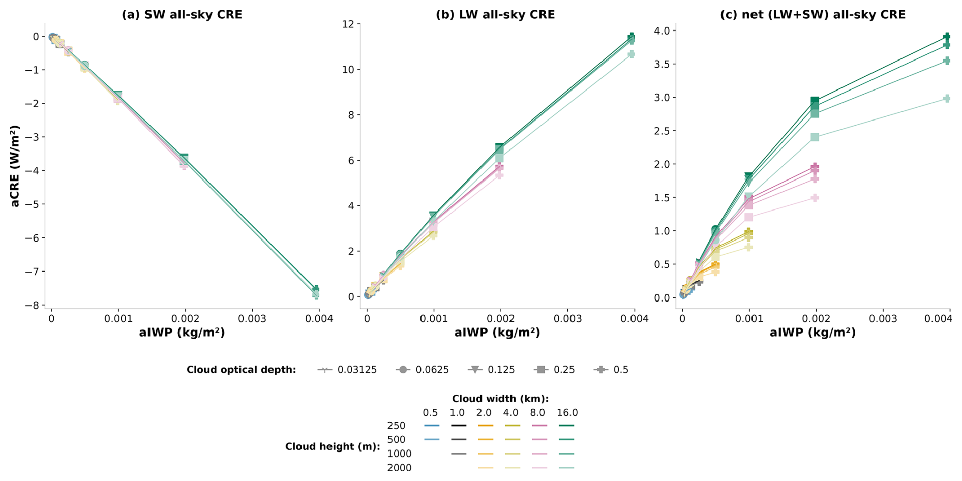
Figure 2a shows the SW aCRE of all cloud configurations as a function of the domain-averaged ice water path (aIWP) for the Sun at zenith. Clouds reflect a larger fraction of solar irradiance back to space than the surface, resulting in a cooling effect for the atmosphere and surface below them. The SW aCRE exhibits a remarkable linear increase with ice content. There is notably very little to no spread between the curves of all cloud configurations, i.e., almost no dependence of the aCRE on cloud geometry.

Figure 2 All-sky cloud radiative effect (a) in the LW, (b) in the SW, and (c) net (SW + LW) as a function of the domain-averaged ice water path for the Sun at zenith. The colors correspond to cloud width w between 500 m (black) and 16 km (green), and the shades correspond to cloud height h (the darkest shade for clouds 250 m thick and lightest for 2 km thick cloud, illustrating that the ice water content goes from densest to lightest). The calculations are done with the ICA and the radiative effects are domain-averaged (in W m⁻² of the domain). Symbols indicate the cloud optical depth.

This behavior can be explained by assuming a linear relationship between cloud reflectance and optical depth for very thin clouds (τ_cloud≪1): R_cloud∝τ_cloud. The cloud optical depth of a homogeneous cloud is proportional to its ice water path (${\mathit{\tau }}_{\mathrm{cloud}}\propto \frac{\mathrm{aIWP}}{w/L}$). Thus, by multiplying cloud reflectance by cloud fraction (i.e., $w/L$) to get a domain reflectance, one finds that the domain reflectance is directly proportional to the total mass of ice it contains:

$$\begin{array}{}\text{(2)}& R_{\mathrm{domain}}\propto R_{\mathrm{cloud}}w/L\propto \mathrm{aIWP}.\end{array}$$

As the SW aCRE is proportional to the domain reflectance (aCRE${}_{\mathrm{SW}}={\mathit{\mu }}_{\mathrm{0}}{F}^{\downarrow }{R}_{\mathrm{domain}}$ with μ₀ the cosine of the solar zenith angle and F^↓ the incident solar flux at cloud top at zenith), it inherits the proportionality to the total mass of ice.

The above relationship is built on the assumption of linearity between cloud reflectance and optical depth. This linearity is observed in htrdr for values of τ_c up to 4 (Fig. 3a) and might be attributed to the scattering phase function of ice crystals, which exhibits a strong peak in the forward direction, adding to the forward radiation as if scattering had not occurred, thereby artificially reducing the “effective” cloud optical depth. Scaling τ_c by a factor (1−g) helps account for the large fraction of forward-scattered radiation (Pierrehumbert, 2010). We seek to determine whether this behavior can be reproduced using simple expressions in such a domain of validity in terms of cloud optical depth. There are many theoretical calculations of cloud reflectance in the literature, some of which reproduce the observed linearity of the CRE with ice content well, but often with an overestimated slope, while others do not even capture the linear relationship (see Fig. C1 in Appendix C). An expression that fits the htrdr results very well can be derived from the two-stream approximation, assuming conservative scattering in the SW (i.e., a single-scattering albedo ω₀=1):

$$\begin{array}{}\text{(3)}& R_{\mathrm{cloud}}={\displaystyle \frac{\mathrm{1}}{\mathrm{1}+{\mathit{\gamma }}_{\mathrm{1}}{\mathit{\tau }}_{\mathrm{c}}}}[{\mathit{\gamma }}_{\mathrm{1}}{\mathit{\tau }}_{\mathrm{c}}+({\mathit{\gamma }}_{\mathrm{3}}-{\mathit{\gamma }}_{\mathrm{1}}{\mathit{\mu }}_{\mathrm{0}}\left)\right(\mathrm{1}-e^{-{\mathit{\tau }}_{\mathrm{c}}/{\mathit{\mu }}_{\mathrm{0}}}\left)\right]\end{array}$$

when using the “hybrid modified Eddington-delta function” method for the coefficients γ₁ and γ₃ (Meador and Weaver, 1980, hereafter MW80). The coefficients are functions of the asymmetry parameter g, the single-scattering albedo ω₀, and the cosine of the solar zenith angle μ₀ (see Appendix C1).

Figure 3 Overcast cloud radiative effect in the (a) SW, (b) in the LW, and (c) net (SW + LW) as a function of cloud optical depth. Calculations done with htrdr using the ICA are in identical colors as in Fig. 2. Compared with Fig. 2, all curves overlap because the oCRE is independent of cloud width. Symbols indicate cloud optical depth. The oCRE approximated with the simple model is plotted as black lines.

As γ₁ and γ₃ do not depend on the cloud optical depth, a Taylor expansion of Eq. (3) gives R_cloud∝τ_c for τ_c≪1. However, this linearity persists for the whole range of studied optical depths up to τ_c=4. For the ice crystals considered here (g∼0.8), the scaled optical depth ${\mathit{\tau }}_{\mathrm{scaled}}=(\mathrm{1}-g){\mathit{\tau }}_{\mathrm{c}}$ extends the validity range of the linear approximation.

In summary, in the SW, the oCRE increases linearly with cloud optical depth up to 4, and, from a domain point of view, the two opposite effects of increasing cloud fraction and decreasing cloud optical depth when spreading a cloud of fixed ice mass perfectly compensate for each other in the aCRE. This results in the SW aCRE being almost independent of cloud geometry for a given mass of ice.

3.1.2 Longwave radiative effect

Figure 2b shows the LW aCRE of all cloud configurations as a function of the domain-averaged ice water path (aIWP). As expected, the longwave radiative effect of clouds is positive and, for a given cloud geometry, increases with aIWP. A rapid linear increase at small aIWP is followed by a slower increase in all cases. There is also a dependence on cloud geometry, mainly on cloud width and, to a much lesser extent, cloud thickness. For example, considering the three groups of points located at aIWP=0.008 kg m⁻², marked by a vertical line, and moving up from one group of points to another, the cloud width increases from 4 (yellow) to 8 (pink) to 16 km (green), and the LW aCRE increases first by more than 60 %, followed by another 40 % (7.8 to 12.9 to 18.2 W m⁻²). For a constant aIWP, when spreading a cloud with a given ice mass, cloud fraction increases and cloud optical depth decreases. Separately, these two mechanisms have opposite effects on the aCRE: an increase in cloud fraction leads to an increase in aCRE, while a decrease in cloud optical depth decreases the aCRE. The positive effect on the LW aCRE of spreading the cloud dominates over the negative effect of reduced cloud optical depth.

One can look at the LW aCRE in more detail which, neglecting the effect of scattering by ice crystals and assuming an isothermal cloud, is given by

$$\begin{array}{}\text{(4)}& {\mathrm{aCRE}}_{\mathrm{LW}}=f\underset{\mathit{\nu }}{\int }{A}_{\mathit{\nu }}[F_{\mathit{\nu }}^{\uparrow }-B_{\mathit{\nu }}(T_{\mathrm{cloud}}\left)\right]\mathrm{d}\mathit{\nu },\end{array}$$

where B(T) is the Planck irradiance at temperature T, A the absorptivity of the cloud, and F^↑ the upward longwave flux at cloud base. The integral term corresponds to the oCRE and strongly depends on cloud optical depth (Fig. 3b). This dependence is expressed through the absorptivity, which can be reproduced with a simple expression by assuming a spectrally constant absorption, neglecting the effect of scattered radiation and using the diffuse approximation:

$$\begin{array}{}\text{(5)}& A=\mathrm{1}-e^{-{\mathit{\tau }}_{\mathrm{c}}(\mathrm{1}-{\mathit{\omega }}_{\mathrm{0}})/\stackrel{\mathrm{‾}}{\mathit{\mu }}}.\end{array}$$

The cloud optical depth τ_c is scaled by a factor 1−ω₀, giving the absorption optical depth. A value of ω₀=0.6 is taken here (see Appendix D), in accordance with the single-scattering properties of ice crystals. $\stackrel{\mathrm{‾}}{\mathit{\mu }}$ is the diffusivity factor of 0.6 (Elsasser, 1942). The approximated LW oCRE is close to that obtained with htrdr: it captures the strong increase at low optical depths followed by the weakened slope, caused by the exponential term in cloud absorption (Fig. 3b). At optical depths larger than 4 (not shown in the figure), the slope decreases further and the LW oCRE saturates.

At low optical depths, the cloud absorptivity (and therefore the oCRE) varies linearly with the cloud optical depth, leading to the same linearity with aIWP in the LW aCRE as observed in the SW aCRE (Fig. A1 in Appendix A) and for an identical reason, but for a shorter range of optical depths below 0.5. In the LW, the optical depth is scaled with (1−ω₀) to remove scattering from the absorption term. The difference between SW and LW lies in the difference in “effective” cloud optical depth, materialized by the terms in the exponential in the expressions for reflectance and absorption. In the SW, $(\mathrm{1}-g)\sim \mathrm{0.2}$, whereas in the LW, $(\mathrm{1}-{\mathit{\omega }}_{\mathrm{0}})/\stackrel{\mathrm{‾}}{\mathit{\mu }}\sim \mathrm{0.67}$. This results in different limit behaviors between the two spectral domains. In general, due to the complexity of scattering, SW CRE is harder to approximate and analyze than LW CRE.

The LW radiative effect slightly depends on the vertical extent of the cloud. In Fig. 2b, for a constant aIWP, geometrically thin clouds (dark curves) are associated with larger aCREs than thicker ones (light curves), indicating that the LW aCRE decreases with increasing vertical extension. This effect can be explained by the dependence of longwave emission on temperature: two clouds sharing cloud-top height and optical depth but with different base altitudes cover different ranges of atmospheric temperature profiles. As temperature decreases with altitude in the troposphere, the cloud with the lower base is distributed over warmer temperatures, therefore emitting more radiation than a cloud with a higher cloud base and reducing the LW aCRE.

3.1.3 Net radiative effect

The behavior of the net CRE is driven by the subtle balance between the SW and LW CRE, making estimation of the sign of instantaneous radiative effect of contrails or cirrus clouds sensitive to small numerical differences. As detailed previously, both SW and LW aCRE increase linearly at low cloud optical depths, with the LW aCRE showing a steeper slope than the SW. For higher cloud optical depths, the slope of the LW aCRE starts decreasing while the SW aCRE remains linear.

Despite the SW and LW aCRE being close to linear for low optical depths, as they nearly cancel each other, small nonlinearities add up and their linearity is not completely reflected in the net aCRE (this is visible in Fig. A1, which is equivalent to Fig. 2 with only the points where τ_c<1). As a result, the net aCRE is initially positive and increasing and then starts to decrease and eventually change sign to become negative at higher contents (Fig. 2c).

Because of its dependence in aIWP, cloud geometry also plays an important role in the net aCRE. For a given aIWP, a progressive horizontal spreading of clouds leads to an enhanced warming or reduced cooling, depending on the sign of the CRE (Fig. 2c), following the behavior of the LW aCRE. Within a critical range of aIWP, the sign of the aCRE becomes dependent on the characteristics of the cloud; i.e., two clouds with identical mass of ice can exert either a positive or a negative radiative effect on the domain, depending on their horizontal geometry. Vertical extension plays a role via the LW contribution but remains weak compared to the other effects.

To summarize, the aCRE changes from positive values for low values of aIWP to negative values for higher values of aIWP. The value at which the sign changes depends strongly on cloud fraction.

3.2 Three-dimensional radiative effects at zenith

The previous section gave an overview of the radiative effect of an idealized cloud calculated using the independent column approximation. Three-dimensional effects of radiation were intentionally ignored. Under the independent column approximation, no radiation is allowed to travel horizontally between clear and cloudy sky: photons can only escape the cloud through its base or top. In other words, the impact of the cloud sides on photon transport is neglected. From this section on, horizontal transport of radiation is taken into account in the simulations, allowing us to compare against ICA results and study the influence of these effects on the CRE.

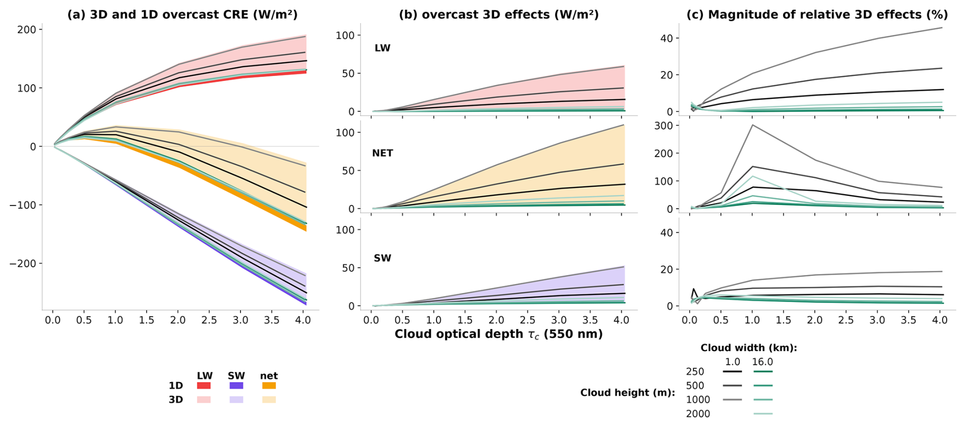
Figure 4 (a) Overcast cloud radiative effect, in W m⁻², as a function of cloud optical depth. Dark lines represent 1D calculations, and light shadings show the range of 3D calculations for various cloud heights and widths. Red is for LW, purple for SW, and orange for net (SW + LW) CRE. Black and green lines correspond to two cloud configurations with 1 and 16 km width, respectively. They both come in different shades, from dark to light, to represent the cloud height h between 250 m and 2 km. (b) 3D effects, i.e., the difference between 3D and 1D oCREs in W m⁻². Light shadings represent the range of the 3D effects, and the black and green lines are as in the first panel. (c) Relative difference between 3D and 1D calculations for each spectral domain: LW on top, SW in the bottom row, and net in the middle.

Figure 4a shows the oCRE of the different cloud configurations for 1D and 3D calculations for the Sun at zenith. Accounting for 3D effects in simulations does not modify the qualitative behavior of the oCRE. However, in both spectral domains, the range of 3D calculations is more positive than that of the 1D, indicating that the 3D effects, i.e., the difference between 3D and 1D CREs, are positive (heating effect). In the LW, the warming effect of clouds is enhanced by 3D effects: unlike in ICA calculations, radiation emitted by the surface and atmosphere below the cloud can be absorbed by cloud sides. Cloud sides also become sources of emission: they emit at cloud temperature, i.e., less energy than the surrounding upwelling radiation coming from the lower and warmer atmosphere and surface. These additional sources of absorption and emission modify the CRE by reducing the outgoing LW radiation. In the SW with the Sun at zenith, incident solar radiation entering the cloud can be scattered through the sides towards the surface. In 1D, these photons would stay within the cloud and therefore have a higher probability of being sent back to space after one or several scattering events. This results in a decreased proportion of reflected radiation in the 3D calculations, equivalent to a reduction in the SW upward flux. Hence, for the Sun at zenith, 3D effects lead to a reduction of the upwelling radiation above the cloud in both spectral domains, adding up to a positive, warming component to net CRE.

Whereas the oCRE is well understood in ICA calculations, 3D calculations add complexity and extra degrees of freedom. Hence, the range of values taken by the oCRE in 3D calculations is very large compared to the 1D calculations. For instance, the effect of cloud geometrical thickness on 3D effects is illustrated in Fig. 4: for all cloud widths and cloud optical depths, geometrically thicker clouds exert larger 3D effects.

It is interesting to note that the effect of cloud geometrical thickness is opposite in 1D and 3D computations of the LW oCRE. We previously showed that for 1D calculations, geometrically thick clouds have a weaker LW oCRE than thin clouds because of their lower cloud base and therefore warmer temperatures. In 3D, as the cloud vertically spreads, the surface of its sides increases, thus enhancing 3D effects and therefore the LW oCRE. For the configurations studied here, this behavior dominates the opposing 1D effect, and the overall effect of cloud height is positive in 3D.

The effect of thickness does not contribute equally to CREs of all clouds geometries: it can double the CRE of narrow clouds (black lines, 1 km width), whereas it has very limited impact on the CRE of wide clouds (green lines, 16 km width). This is because cloud thickness needs to be compared to its width. The aspect ratio (geometrical thickness to width) of the 16 km wide cloud is very small. The contribution of cloud sides in the CRE is thus small relative to its wide surface. As a result, the magnitude of 3D effects becomes negligible relative to the net oCRE. When considering the influence of the cloud on the whole domain, i.e., the aCRE instead of the oCRE, we determine from empirical analysis that in the LW, 3D effects are nearly insensitive to cloud width and they depend almost linearly on the product of cloud optical depth and height (CRE${}_{\mathrm{LW}}^{\mathrm{3}\mathrm{D}}-{\mathrm{CRE}}_{\mathrm{LW}}^{\mathrm{1}\mathrm{D}}\propto {\mathit{\tau }}_{\mathrm{c}}\times h$, Fig. 5b). As cloud optical depth is proportional to the aIWP-to-cloud-width ratio (${\mathit{\tau }}_{\mathrm{c}}\propto \mathrm{aIWP}/w$), we can establish that 3D effects in the LW increase linearly with the product of aIWP, cloud width, and height (${\mathrm{CRE}}_{\mathrm{LW}}^{\mathrm{3}\mathrm{D}}-{\mathrm{CRE}}_{\mathrm{LW}}^{\mathrm{1}\mathrm{D}}\propto \mathrm{aIWP}/w\times h$). This relationship works for the LW spectrum but it appears that those parameters are not sufficient to determine the behavior of 3D effects in the SW (Fig. 5a).

Thus, when looking at the aCRE, 3D effects of radiation are dependent on cloud height and indirectly on cloud width via the optical depth (because ${\mathit{\tau }}_{\mathrm{c}}\propto \mathrm{aIWP}/w$). When considering the oCRE, the cloud width is introduced directly in the equation ($\mathrm{oCRE}\propto \mathrm{aCRE}/w$), hence introducing the aspect ratio indirectly.

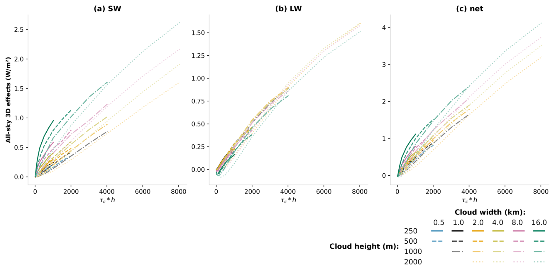
Figure 5 (a) SW, (b) LW, and (c) net all-sky 3D effects in W m⁻² as a function of the product of cloud optical depth and cloud height τ_c×h. The colors and line styles are as in Fig. 1.

Three-dimensional effects can have a great impact on the net CRE. For optically thin clouds which have a net CRE close to 0 under the independent column approximation, 3D effects can be of the same magnitude as the 1D CRE itself. For some cloud optical depths, two cloud geometries can exhibit net oCRE of opposite signs because of 3D effects (Fig. 4a).

4 Dependence on solar zenith and azimuth angles

The sensitivity of the CRE to solar zenith and azimuth angle is now investigated. For the sake of simplicity, we choose a fixed cloud configuration with a width of 1 km and height 0.5 km. Three cloud optical depths of 0.25, 1, and 4 are selected to pursue our prior analysis of the behavior of the CRE of optically thin clouds. Solar zenith angle (SZA) is varied between 0 and 88°, and solar azimuthal angle can take two values: 0 and 90°. Cloud dimensions are similar to that of Gounou and Hogan (2007) to allow comparison with their results. The LW CRE has no dependence on SZA as the temperature profile is kept constant.

4.1 Independent column approximation

We start with the analysis of independent column calculations. Figure 6a shows the SW oCRE as a function of SZA for several cloud optical depths, obtained with htrdr with the independent column approximation (crosses) and with Eq. (3) (solid lines). Let us focus first on low optical depths, i.e., τ_c=0.25 (purple lines). In the SW, the cooling effect of the cloud strengthens with increasing SZA before reaching a maximum at large angles (70–80°) and declining towards zero when the Sun gets close to the horizon (Fig. 6a). Two opposing effects are at play in the SW when the Sun goes down on the horizon: decreasing incident solar radiation, following the cosine of zenith angle μ₀, and increasing cloud reflectivity R(μ₀).

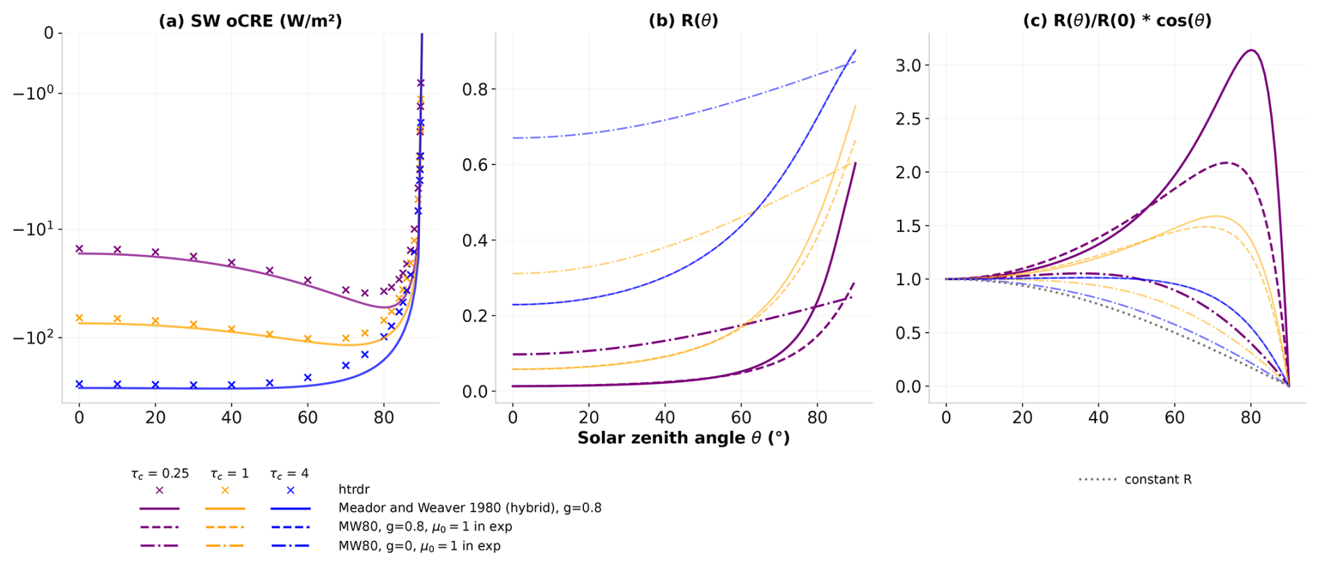
Figure 6 (a) SW overcast cloud radiative effect, in W m⁻², as a function of solar zenith angle θ for a cloud with width 1 km and height 500 m. Lines denote Meador and Weaver (1980) approximations and crosses denote htrdr calculations using the ICA. Three cloud optical depths are shown: 0.25 in purple, 1 in yellow, and 4 in blue. Note the logarithmic scale on the y axis. (b) Cloud reflectivity and (c) ratio of cloud reflectivity to cloud reflectivity at zenith multiplied by the cosine of solar zenith angle, for several approximations, as a function of solar zenith angle. Colors are as in (a). Dashed lines show MW80 with μ₀=1 in the exponential term, and dash-dotted lines show MW80 with both μ₀=1 and g=0. The dotted gray line in (c) illustrates the case of constant reflectivity, i.e., cos (θ).

Once again, we use MW80 to analyze the behavior of the CRE, as it provides a good approximation of the dependence of reflectivity on SZA (Eq. 3). This increase is driven by μ₀ via two components; the first is the dependence of extinction on the path taken by incident solar radiation within the cloud (the exponential term in Eq. 3), and the second is the angular dependence of scattering properties (influenced by the asymmetry parameter, g). The impact of these two components of cloud reflectivity can be distinguished by successively taking a constant μ₀=1 in the exponential term of Eq. (3) and then setting g=0 in the γ₁ and γ₃ parameters. Figure 6b displays the reflectivity as a function of SZA, and panel (c) shows the product of cloud reflectivity and cosine of the zenith angle, i.e., the combination of the two components of SW CRE. For optically thin clouds (τ_c=0.25), the μ₀=1 curve (dashed line) shows a pronounced attenuation of the strong peak at large SZAs that exists using the unmodified MW80 expression (solid line) and obtained with htrdr. This difference can be attributed to the absence of an increase in extinction resulting from setting a constant μ₀. The remaining increase in cloud reflectivity in the μ₀=1 curve can be attributed to the angular dependence of scattering effects, explained by the strong forward peak of the ice crystal scattering phase function. When the Sun is at zenith, scattering directions towards the surface are favored. For increasing zenith angles, the probability of forward scattering is unchanged but the scattering direction follows the SZA, resulting in a larger fraction of radiation being upscattered. This angular dependence of upscattering has been studied by Wiscombe and Grams (1976) among others and can be highlighted by comparing to a computation where the asymmetry factor g is set to 0. The resulting phase function is symmetrical and the angular dependence of upscattering is dampened. The obtained reflectivity, illustrated by the dash-dotted lines in Fig. 6b and c, clearly shows the absence of the previously observed peak at large zenith angles. It is interesting to note in panel (b) that (1) as the g=0 reflectivity has a weaker angular dependence, its value at zenith is larger than MW80, and (2) despite the higher value at zenith and a mild increase with increasing zenith angle, its value at 90° is still lower than the MW80 reflectivity. For illustrative purposes, a constant reflectivity is added in panel (c) (dotted line). The g=0 curve is close to the constant reflectivity curve, and only small angular dependence remains due to the g=0 phase function not being perfectly isotropic and thus still having a small angular dependence.

The maximum reached by the SW CRE at large SZA is specific to small cloud optical depths. As the cloud optically thickens, the reflectivity for the Sun at zenith increases and its angular dependence is diminished. As a result, the SW CRE reaches its maximum closer to zenith. The μ₀=1 curve does not differ from the regular MW80 curve any longer. The increase with zenith angle of the path taken by incident solar radiation within the cloud has no effect any more. The remaining observed angular dependence of reflectivity is attributed to scattering properties only.

4.2 Variation of 3D effects with solar position

Three-dimensional effects of radiation influence how SW CRE depends on the position of the Sun. Under the independent column approximation, the azimuth angle has no influence on the SW CRE as the cloud is seen as infinite in both x and y horizontal directions. In 3D calculations, however, the orientation of the Sun relative to the cloud needs to be accounted for. Figure 7 shows the 3D SW oCRE for two azimuth angles, corresponding to two orientations of the Sun: perpendicular (ϕ=0, dashed line) and parallel (ϕ=90, dotted line) to the cloud. Focusing first on low cloud optical depth, τ_c=0.25. For zenith angles from θ=0° to about θ=75°, 3D effects are positive. Qualitative behavior when 3D radiative effects are included is similar to that for the 1D calculations: increase in SW CRE with increasing SZA, maximum located at large SZA, and decrease to 0 at θ=90°. The location and magnitude of the maximum CRE, however, differ and depend on azimuth angle. When the Sun is low on the horizon and in a direction parallel to the cloud, 3D radiative effects tend to zero and 1D and 3D give almost the same results. In contrast, when the Sun is perpendicular to the cloud, the maximum of SW CRE is larger in the 3D case and happens at a larger SZA than the 1D case (around θ=85°), leading to negative 3D effects that can account for up to several hundred percent of the SW CRE. The divergence in 3D effects based on cloud orientation relative to the Sun can be interpreted with clarity. On one hand, the “parallel-Sun” 3D case is geometrically similar to the 1D approximation, with the Sun seeing a contrail of infinite length parallel to its rays. In both scenarios, most of the radiation goes into the contrail and very little is scattered through the sides, yielding weak 3D effects. On the other hand, when the Sun is perpendicular to the contrail, and especially when it goes down on the horizon, an increasing fraction of cloud sides is sunlit, increasing its effective cover and resulting in enhanced 3D effects and SW CRE.

The zenith angle at which 3D effects change sign to become negative in the perpendicular configuration depends on the cloud optical depth. It decreases from θ∼75° for τ_c=0.25 to θ∼45° for τ_c=4.

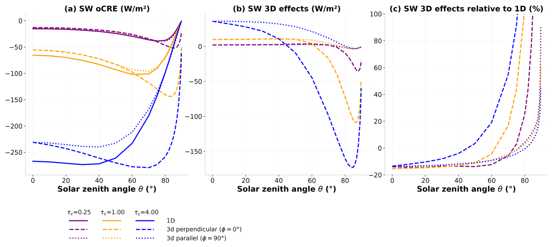
Figure 7 (a) SW overcast cloud radiative effect, (b) SW 3D effects in W m⁻², and (c) SW 3D effects relative to 1D calculations in percent as a function of solar zenith angle θ. The solid lines denote htrdr calculations using the independent column approximation. The dashed and dotted lines correspond to 3D calculations, with an azimuth angle of 0 and 90°, respectively. Three cloud optical depths are shown: 0.25 in purple, 1 in yellow, and 4 in blue. The calculations are for the cloud with 1000 m width and 500 m height. Note the logarithmic scale on the y axis.

4.3 Sensitivity to cloud shape

To investigate the impact of our choice of a rectangular cross-section for the cloud, experiments were repeated with an elliptical contrail. We chose a configuration close to the one studied in Gounou and Hogan (2007), hereafter GH07, with a width of 800 m, height of 400 m, and mean optical depth of 0.2 and 0.4. The ice water content (IWC) depends on the distance to the center of the contrail, with a peak IWC at the center, as in GH07:

$$\begin{array}{}\text{(6)}& \mathrm{IWC}=\left\{\begin{array}{ll}{\mathrm{IWC}}_p\cos \left(\frac{\mathit{\pi }}{\mathrm{2}}r\right)& \text{for }r<\mathrm{1};\\ \mathrm{0}& \text{for }r\ge \mathrm{1},\end{array}\right.\end{array}$$

where

$$\begin{array}{}\text{(7)}& r={\left[{\left({\displaystyle \frac{x-x_{\mathrm{0}}}{\mathrm{\Delta }x/\mathrm{2}}}\right)}^{\mathrm{2}}+{\left({\displaystyle \frac{z-z_{\mathrm{0}}}{\mathrm{\Delta }z/\mathrm{2}}}\right)}^{\mathrm{2}}\right]}^{\frac{\mathrm{1}}{\mathrm{2}}}.\end{array}$$

IWC_p is the maximum ice water content at the center of the cloud, (x₀,z₀) the position of the center of the cloud, and Δx and Δz the geometrical width and thickness of the cloud. To separate the effects of IWC inhomogeneity and cloud shape, we also ran experiments with an ellipse of uniform IWC. We end up with three types of clouds with the same mean optical depth: the rectangle cloud with uniform IWC and optical depth, the uniform ellipse with uniform IWC and inhomogeneous optical depth, and the GH07 ellipse with inhomogeneous IWC and optical depth. The three configurations show different degrees of inhomogeneity in terms of IWC and cloud optical depth.

The CREs of the three configurations are very similar in both 1D and 3D (Fig. 8). In the LW and in the SW at zenith, differences between the ellipse and the rectangular cloud CREs are very small. The LW oCRE of the GH07 ellipse is slightly weaker, i.e., less warming than that of the rectangular cloud, by less than 5 %. The SW oCRE at zenith shows a small difference: the CRE of the GH07 ellipse exhibits a stronger cooling of about 0.5 W m⁻², i.e., 2.5 %. At larger zenith angles, larger differences appear, where the rectangular cloud (uniform ellipse) is up to 15 % (10 %) more cooling than the GH07 ellipse above 80°. For the net oCRE, this results in a GH07 ellipse less warming than the others at zenith and less cooling at large zenith angles where the net oCRE is negative. The delta oCRE changes sign at some point, but around the same point the net oCRE also changes sign.

In terms of cloud optical depth inhomogeneity, differences are negligible in the LW and in the SW with the Sun at zenith, but for large SZAs, the SW oCRE increases as cloud optical depth becomes more homogeneous. Also, the differences between uniform and nonuniform clouds are more pronounced than between ellipses and rectangular clouds, which means that here, inhomogeneity seems to be more important than the cloud shape for the CRE, via optical depth effects (and therefore scattering) at the sides of the clouds.

But importantly, the three configurations show 3D effects of similar magnitude. Thus, the choice of a homogeneous rectangular cloud does not change the behavior of the CRE or 3D effects and even facilitates the analysis.

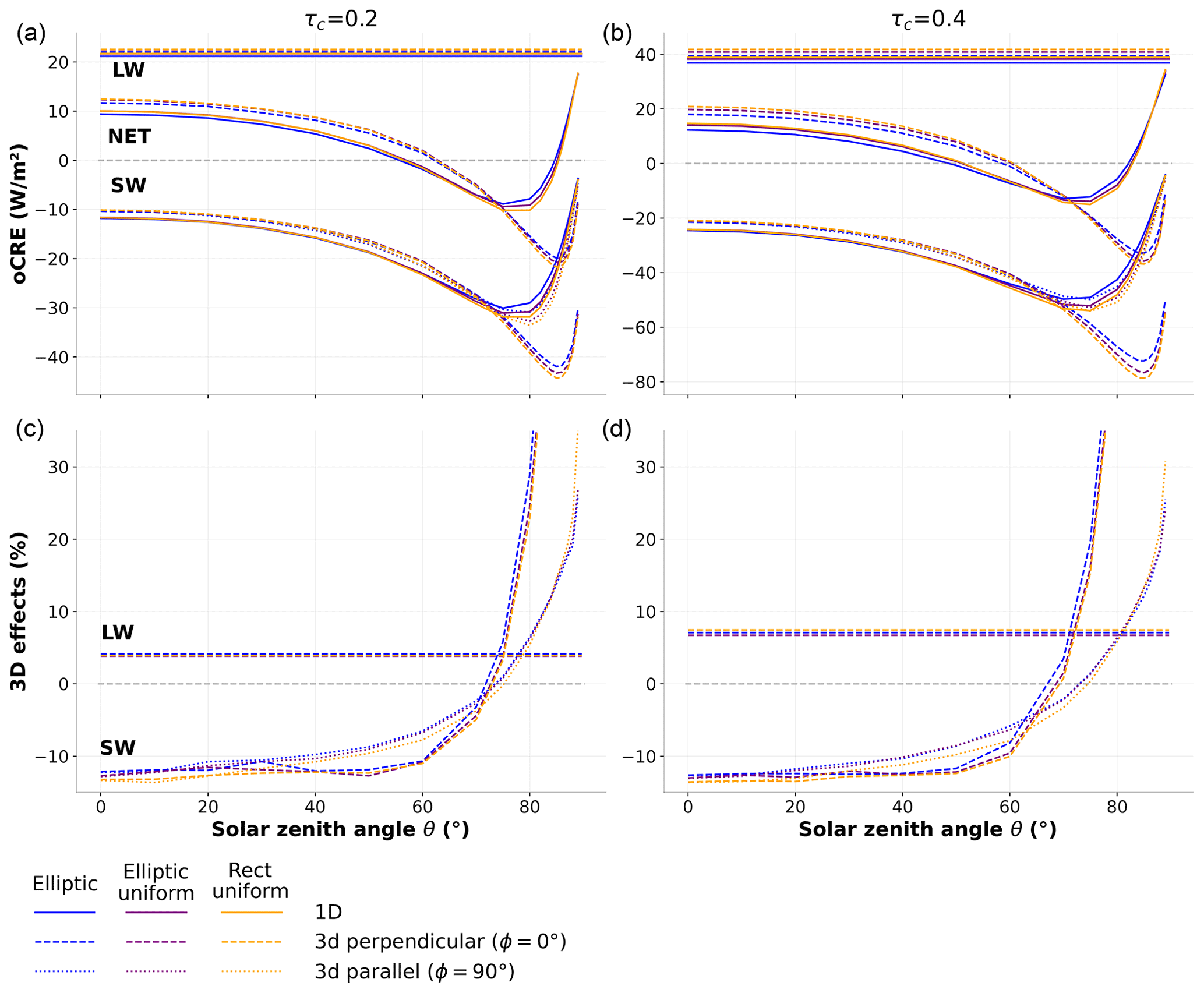
Figure 8 (a, b) LW, SW, and net oCRE (in W m⁻²) as a function of solar zenith and azimuth angles for a 800 m wide and 400 m thick cloud and for a cloud optical depth of 0.2 (a, c) and 0.4 (b, d). (c, d) LW and SW 3D effects relative to 1D calculations in percent. Clouds with an elliptic shape and inhomogeneous IWC are in blue, an elliptic shape with uniform IWC in purple, and a rectangular shape with uniform IWC in orange.

5 Temporal integration of the CRE and 3D effects

In the previous sections we calculated the sensitivity of the CRE to the Sun zenith and azimuth angles. In this section, we assess how CRE and 3D effects behave when integrated in time on a specific day and location. This allows a better representation of real-life scenarios where all solar angles do not have equal weights. The usual method to calculate a daily mean is to fit the curve of the CRE as a function of the solar zenith and azimuth angles, followed by integrating the obtained curve over zenith and azimuth angles in accordance with their distribution throughout the day. However, Monte Carlo methods offer another way, since they consist of statistical evaluation of integrals. The introduction of an additional integration dimension, in this case over the Sun zenith and azimuth angles, is equivalent to adding one random sampling per photon path, with minimal impact on numerical complexity. With this approach, time integration is performed without increasing computational time (Nyffenegger-Péré et al., 2024). In order to achieve this, a solar position is sampled for each sampled photon, thus allowing the daily and spectral, spatial, angular, and photon path integrations to be performed simultaneously. Daily averages of the CRE and 3D effects are calculated for a number of dates and locations. Two latitudes and three dates are considered, namely 45 and 60°, equinoxes, and winter and summer solstices; the corresponding Sun paths are illustrated Fig. 9.

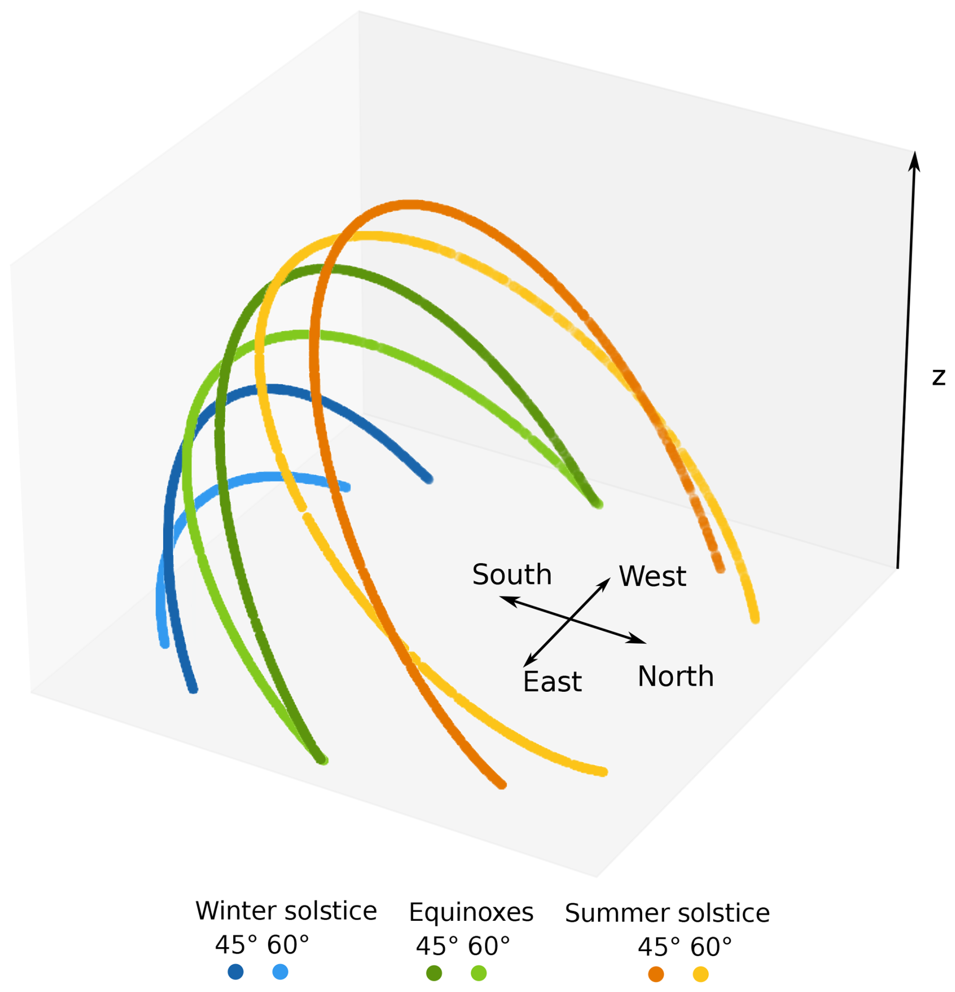
Figure 9 Illustration of Sun paths for selected dates and locations. The summer solstice is in orange, equinox in green, and winter solstice in blue. In the examples shown here, the Sun reaches the lowest zenith angle (i.e., the highest position in the sky) during the summer solstice at 45° latitude. See also Fig. E1.

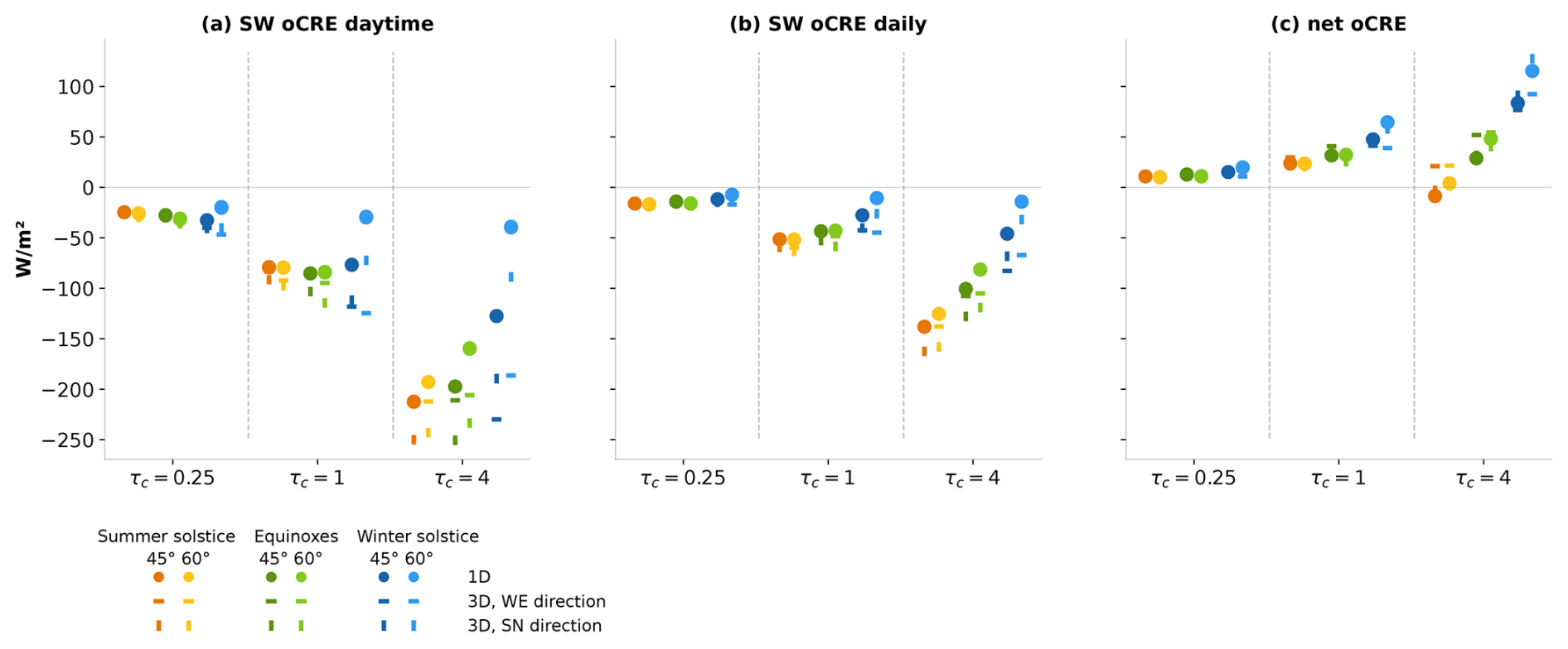
Figure 10 Mean (a) SW daytime, (b) SW daily, and (c) net oCRE for selected days, latitudes, cloud optical depths, and cloud orientations. Dots denote the 1D calculations and dashes the 3D calculations: horizontal (vertical) dashes are for W–E-oriented (S–N-oriented) clouds. In each panel are three groups of points corresponding to the three studied cloud optical depths. In each group, from left to right, is the summer solstice, equinox, and winter solstice. Dark colors are for 45° latitude and lighter colors for 60° latitude. The calculations are for a rectangular cloud with 1000 m width and 500 m height.

Figure 10a shows the mean daytime CRE, i.e., the CRE averaged between sunrise and sunset, for the selected days and latitudes and three cloud optical depths. As before, mean SW CRE increases with cloud optical depth. The impact of latitude and day of the year varies depending on cloud optical depth: for the thinnest cloud (τ_c=0.25), SW CRE roughly increases with the day of the year and latitude (from summer solstice to equinox to winter solstice and from 45 to 60° of latitude), whereas in the cloud with optical depth of 4, effects are more pronounced and in the opposite direction. This can be understood by examining the distribution of solar angles in each configuration and focusing first on the 1D calculations. As the day of the year progresses from the summer solstice to equinox and then to winter solstice, solar zenith angles increase (Fig. E1 in Appendix E). The winter solstice especially stands out from the other days because its SZAs remain larger than 80°, whereas only about 20 % of SZAs are that low in the other configurations. Therefore, the mean daytime SW CREs over the year exhibit a similar pattern to that observed in Fig. 7: for the thinnest cloud with optical depth 0.25, an initial increase in the SW CRE with zenith angle is followed by a decrease to zero after reaching a maximum at a high zenith angle around 80°. For the thickest cloud with τ_c=4, Fig. 7 shows a maximum CRE at zenith before slowly decreasing to zero. As a consequence, the mean CRE of the τ_c=4 cloud peaks in summer and decreases on the other days of the year according to the distribution of angles.

Daily mean SW CRE is obtained by multiplying daytime SW CRE by daytime fraction, as plotted in Fig. 10b, having the effect of reducing the magnitude of the SW CREs, especially during the winter solstice and equinoxes. Finally, the net daily effect can be calculated by adding up the LW CRE, which in the majority of cases yields a positive result (Fig. 10c).

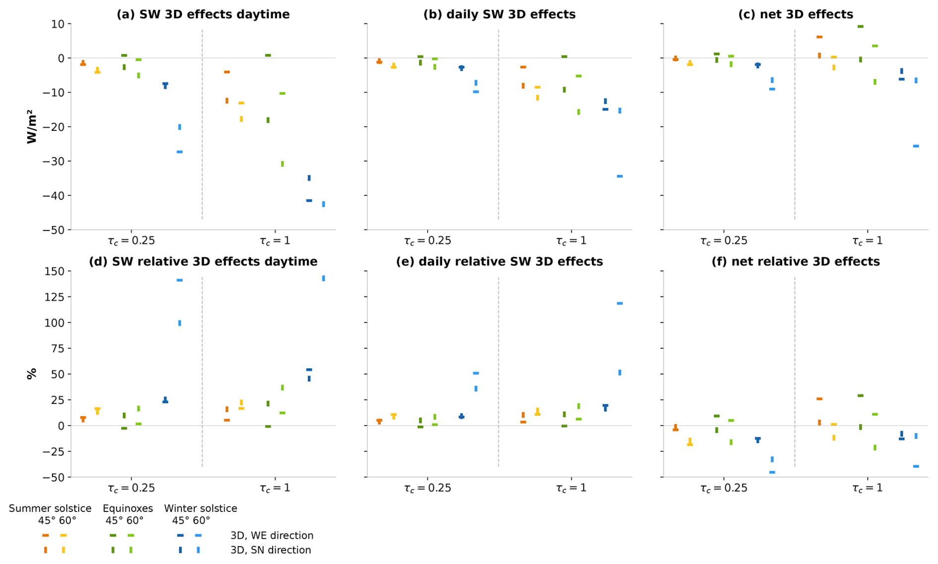
Figure 11 Mean (a) SW daytime, (b) SW daily, and (c) net 3D effects, along with (d) SW daytime, (e) SW daily, and (f) net relative 3D effects for selected days, latitudes, cloud optical depths, and cloud orientations. Horizontal (vertical) dashes are for W–E-oriented (S–N-oriented) clouds. In each group, from left to right, is the summer solstice, equinox, and winter solstice. Dark colors are for 45° latitude and lighter colors for 60° latitude. The scale on the y axis has been adjusted to enhance the clarity of the figure; some extreme values have been excluded. The calculations are for a cloud with 1000 m width and 500 m height.

We now focus on 3D effects plotted in Fig. 11, with the top row displaying absolute values and the bottom row showing relative 3D effects. To improve figure clarity, we focus on clouds with optical depths of 0.25 and 1. In the majority of cases, daytime SW 3D effects are negative (Fig. 11a). They increase with increasing optical depth, day of the year (summer solstice to equinox to winter solstice), and latitude. Thus, the largest 3D effects are observed at the winter solstice at latitude 60°. In addition to the dependence on cloud optical depth, day of the year, and latitude, averaged 3D effects also exhibit a dependence on cloud orientation relative to the Sun. Here we again examine two configurations: one with the cloud aligned in a south–north direction and another in a west–east direction. As seen in Sect. 4, 3D effects are influenced by both zenith and azimuth angles (Fig. 7): the largest 3D effects are observed at large zenith angles, when the Sun rays are perpendicular to the cloud. During the summer solstice and equinox, the perpendicular position is more prevalent for the S–N cloud, whereas for the winter solstice, it is more common for the W–E cloud. Given that the perpendicular orientation is associated with pronounced 3D effects at large zenith angles, the largest 3D effects are therefore caused by the S–N cloud during summer solstice and equinox and by the W–E cloud during winter solstice. This behavior is evident in the τ_c=1 (and also for τ_c=4, not shown) and is also exhibited by the thinnest cloud, despite the fact that certain configurations do not show distinct 3D effects (for the summer solstice at both latitudes and the winter solstice at 45° latitude).

Similarly to the SW CRE, switching from daytime to daily SW 3D effects reduces their magnitude but does not change their sign (Fig. 11b). In contrast, adding the positive LW 3D effects to SW 3D effects to obtain net 3D effects yields positive values in some cases (Fig. 11c). The highest relative 3D effects are observed in winter at 60° latitude. Even though they can go above 100 % of the CRE when considering only SW daytime 3D effects, net 3D effects remain under 50 % of the 1D CRE.

6 Conclusions

This paper investigates the sensitivity of the radiative effect of optically thin ice clouds to their geometric properties and optical depth, with a focus on three-dimensional effects of radiation and the subtle balance between SW and LW components of the net CRE. To this end, we use the Monte Carlo radiative transfer code htrdr on a parallelepipedic cloud with varying width, geometrical thickness, and optical depth.

For sufficiently thin clouds and the Sun at zenith, the 1D SW all-sky CRE (aCRE), i.e., the radiative effect of the cloud with neighboring clear-sky parts, can be accurately determined using only the total ice content in a grid box. For a constant total ice content, how cloud fraction and in-cloud ice water path are distributed does not influence SW aCRE. This is also valid for 1D LW aCRE but for a smaller range of optical depths (τ_c⩽0.5).

Simple analytical models reproduce the dependence of LW and SW oCRE on cloud optical depth quite well when taken separately. The LW CRE can be well approximated by a simple, classical model. Conversely, the SW CRE is more challenging to approximate, despite its remarkable linear relationship with cloud optical depth up to τ_c=4, and requires an adequate two-stream approximation. This study highlights the great sensitivity of SW CRE to the simple models found in the literature, a number of which exhibit a wrong slope, including the simple $(\mathrm{1}-g)/\mathrm{2}$ approximation. When the LW and SW are added together to obtain the net CRE, however, small differences are exacerbated and the net CRE is less well reproduced.

As previously shown in the literature (Gounou and Hogan, 2007; Forster et al., 2012), the SW CRE varies significantly with zenith angle and displays different behaviors depending on optical depth. The CRE of very thin clouds reaches a maximum at large zenith angles (θ∼75° for τ_c=0.25), before decreasing to zero when the Sun goes below the horizon. For thickest optical depths, around 4, the CRE is maximum at zenith, follows a plateau, and then begins to decline around θ∼40°. Cloud optical depth determines the zenith angle at which maximum SW CRE is reached: the optically thinner the cloud, the larger the zenith angle of maximum SW CRE.

Three-dimensional effects of radiation are positive in the LW and depend linearly on the product ${\mathit{\tau }}_{\mathrm{c}}\times \frac{h}{w}$, with $\frac{h}{w}$ the cloud aspect ratio, and can therefore be easily approximated for homogeneous clouds. In the SW, 3D effects are positive at zenith, and their behavior at increasing zenith angles largely depends on the position of the Sun relative to the contrail. When the cloud is parallel to the Sun, SW 3D effects are maximum at zenith and decrease to zero with increasing zenith angle. Conversely, when the cloud is oriented perpendicular to the Sun, the SW 3D effects, which are positive at zenith, change sign to become negative and reach a maximum at a large zenith angle. The zenith angle at which SW 3D effects switch sign depends on the optical depth: the optically thinner the cloud, the greater the zenith angle from which the effect turns negative.

The behavior of 3D effects in relation to the position of the Sun naturally gives rise to the question of their value when integrated over the course of a day. Integrating the CRE and 3D effects for selected latitudes (45 and 60°, where high-frequency flight routes and persistent contrails are currently located) and days of the year (equinoxes, solstices), we find that 3D effects resist daily integration in some cases. The Sun–cloud absolute azimuth angle influences the magnitude of the mean 3D effects, with the highest daytime SW 3D effects being in winter at 60° latitude for a cloud oriented in the west–east direction. For summer and equinoxes, the south–north orientation is associated with the highest 3D effects. When considering the net result, positive LW 3D effects that persist day and night help balance the strong negative daytime SW 3D effects. The net 3D effects still end up being significant, particularly when a large fraction of the day is associated with large SZAs, i.e., during winter at high latitudes. The identification of configurations in which 3D effects are most important paves the way for the validation of existing parameterizations of 3D effects (Schäfer et al., 2016; Hogan et al., 2016) or the development of new parameterizations adapted to these particular situations.

The effect of solar position on SW 3D effects has been studied for a cloud with a fixed aspect ratio of $\mathrm{1}/\mathrm{2}$ (a cloud width of 1 km and geometrical thickness of 0.5 km). We expect the SW 3D effects to decrease as the aspect ratio goes to zero, but not linearly. Calculations conducted on a cloud with an aspect ratio of $\mathrm{1}/\mathrm{8}$, i.e., a cloud 4 times larger (width of 4 km and thickness of 0.5 km, with a cloud optical depth of 0.25), show that the daytime integrated SW 3D effects do not decrease by the same amount. This suggests that 3D effects of radiation may still be significant for clouds with small aspect ratios.

Our calculations differ from those of Gounou and Hogan (2007) (GH07) and Forster et al. (2012) (F12) in several respects. There are slight differences between the LW and SW CREs at zenith, which are compensated for in the net CRE. The 3D effects of htrdr are less pronounced than those of GH07 and F12 in the LW. In the SW, however, htrdr produces larger 3D effects than GH07 and F12, particularly at large zenith angles. Overall, htrdr results are more similar to those of F12 than GH07.

We also ran the calculations using Fu (1996) and Fu et al. (1998) optical properties for a radius of 10 µm. The results are similar to what we find with Laurent Labonnote's LUT and are not shown in this paper. In general, we expect that changing the ice crystal shape will affect the magnitude of the CRE and the intensity of its maximum absolute value at large zenith angles via the asymmetry factor. This might also explain the slight differences between our results and those of GH07 and F12.

We have shown that zenith angle plays an important role in the CRE in both 1D and 3D, especially when it becomes very large (θ>85°). However, the Earth's curvature and the solid angle of the Sun, which are usually neglected as we do here, may be non-negligible in this range of solar angles and would need to be taken into account for a correct estimation of the CRE, especially for days or flight trajectories that mostly span large SZAs. Furthermore, this requires the radiative code to accurately calculate scattering even when the phase function has a strong forward peak, which is not necessarily the case with codes developed to be very fast (with the exception of recent methods, e.g., as proposed by Momoi et al., 2022). These effects when the Sun is very low on the horizon are also very sensitive to the representation of the phase function. The use of Henyey–Greenstein has limitations (Boucher, 1998) and might need to be revisited.

This paper does not address the radiative effects of heterogeneity of cloud properties, particularly ice content, beyond the very idealized case studied in Gounou and Hogan (2007) and Forster et al. (2012). Given the importance of nonlinear effects of optical depth on the CRE in terms of both angular dependence and three-dimensional effects, it is reasonable to conclude that such heterogeneities will influence the value of the CRE, therefore requiring a dedicated study.

Finally, in this study, the atmospheric configuration was significantly simplified, particularly with a non-reflecting surface and the absence of neighboring clouds. The tools we used are capable of handling more complex scenarios, and the Monte Carlo approach enables global-scale analysis. However, this will be the focus of a future study. Still, it is probable that 3D radiative effects of optically thin clouds are important in many situations, especially at low SZAs.

Appendix A: Precisions on radiative transfer calculations

When performing radiative transfer calculations, great care must be taken to ensure that the radiative budget is closed by accounting for the radiative effect of all photons, irrespective of their direction of travel. For calculations at zenith, a large horizontal sensor of L=66 km is sufficient to capture radiation, even radiation located far away from the cloud. When the direction of incoming photons from the Sun is no longer vertical, the fraction of photons going to the sides increases significantly. Vertical sensors placed near the cloud are then needed, denoted S₂ and S₃ and depicted in Fig. A1. This creates a “box” that ensure that photons scattered upward with a horizontal component are included in radiative flux calculations. In these situations, the length of horizontal sensor S₁ can be reduced.

It also appears that for the vertical sensors S₂ and S₃, the flux incident to the outer sides of the sensors (indirect flux, which does not come directly from the cloud) should be subtracted to the flux incoming to the inner sides; i.e., a net flux should be calculated for sensors S₂ and S₃. Not accounting for that inward flux causes errors in the magnitude, and even sign, of the integrated 3D effects for some geometries. Hence, five htrdr runs are needed to calculate a SW flux and 10 for a SW CRE (five clear, five cloudy). The five runs are added to give the corresponding total flux:

$$\begin{array}{}\text{(A1)}& F=F_{\mathrm{up}}^{S_{\mathrm{1}}}+{\displaystyle \frac{H_{S_{\mathrm{23}}}}{L_{S_{\mathrm{1}}}}}\left(F_{\mathrm{in}}^{S_{\mathrm{2}}}-F_{\mathrm{out}}^{S_{\mathrm{2}}}+F_{\mathrm{in}}^{S_{\mathrm{3}}}-F_{\mathrm{out}}^{S_{\mathrm{3}}}\right),\end{array}$$

with w the cloud width, $L_{S_{\mathrm{1}}}$ the length of the horizontal sensor, and $H_{S_{\mathrm{23}}}$ the height of the vertical sensors. For consistency, net fluxes at sensors S₂ and S₃ are multiplied by a factor $H_{S_{\mathrm{23}}}/L_{S_{\mathrm{1}}}$ to scale them to the width of sensor S₁. In the calculations in Sect. 4, $H_{S_{\mathrm{23}}}$ is set to 2 km, which is the distance between the altitudes of the cloud top and sensor S₁. $L_{S_{\mathrm{1}}}$ is set to 5 km. For independent column calculations, the second term on the right-hand side of Eq. (A1) is negligible since the size of the horizontal grid is multiplied by a very large number (10⁶), thus giving $L_{S_{\mathrm{1}}}\gg H_{S_{\mathrm{23}}}$.

The overcast CRE and 3D effects are then obtained with the following expressions.

$$\begin{array}{}\text{(A2)}& {\displaystyle }\mathrm{oCRE}=f\times \mathrm{aCRE}={\displaystyle \frac{w}{L_{S_{\mathrm{1}}}}}\left(F_{\mathrm{clear}}-F_{\text{all-sky}}\right)\text{(A3)}& {\displaystyle }\begin{array}{rl}\mathrm{3}\mathrm{D}& ={\mathrm{oCRE}}^{\mathrm{3}\mathrm{D}}-{\mathrm{oCRE}}^{\mathrm{1}\mathrm{D}}\\ & ={\displaystyle \frac{w}{L_{S_{\mathrm{1}}}}}\left[\left(F_{\mathrm{clear}}^{\mathrm{3}\mathrm{D}}-F_{\text{all-sky}}^{\mathrm{3}\mathrm{D}}\right)-\left(F_{\mathrm{clear}}^{\mathrm{1}\mathrm{D}}-F_{\text{all-sky}}^{\mathrm{1}\mathrm{D}}\right)\right]\end{array}\end{array}$$

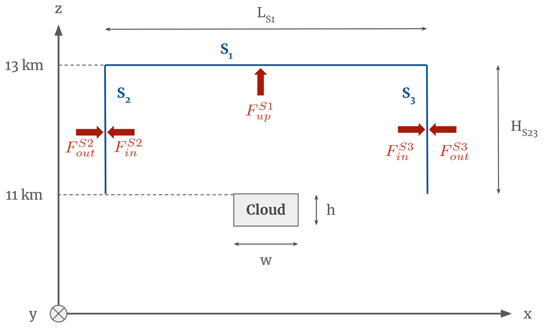
Figure A1 Schematic of the sensors used for the radiative transfer calculations. Sensor S₁ is used for all calculations when the Sun is at zenith, and sensors S₂ and S₃ are used when the solar zenith angle is larger than 0.

Appendix B

Figure B1 is similar to Fig. 2, showing the aCRE of all cloud configurations as a function of the domain-averaged ice water path (aIWP) for the Sun at zenith, except that it only shows configurations with a cloud optical depth below 0.5. This corresponds to the range of quasi-linearity between the aCRE and the aIWP in both spectral domains. As shown in Sect. 3.1, the range of linearity for the SW extends to cloud optical depths up to 4.

Figure B1 Same as Fig. 2, but zooming in on cloud optical depths under 1 to highlight the linearity of LW CRE at these optical depths. SW CRE is also linear for this range of cloud optical depth and above.

Appendix C: Simplified theoretical model

C1 Details on the parameters used for MW80

We recall Eq. (3) for reflectivity:

$$\begin{array}{}\text{(C1)}& R_{\mathrm{cloud}}={\displaystyle \frac{\mathrm{1}}{\mathrm{1}+{\mathit{\gamma }}_{\mathrm{1}}{\mathit{\tau }}_{\mathrm{c}}}}[{\mathit{\gamma }}_{\mathrm{1}}{\mathit{\tau }}_{\mathrm{c}}+({\mathit{\gamma }}_{\mathrm{3}}-{\mathit{\gamma }}_{\mathrm{1}}{\mathit{\mu }}_{\mathrm{0}}\left)\right(\mathrm{1}-e^{-{\mathit{\tau }}_{\mathrm{c}}/{\mathit{\mu }}_{\mathrm{0}}}\left)\right].\end{array}$$

Parameters γ₁ and γ₃ used in this expression come from Meador and Weaver (1980) using the modified Eddington-delta function hybrid method (also in Table C2).

$$\begin{array}{}\text{(C2)}& \begin{array}{rl}& {\mathit{\gamma }}_{\mathrm{1}}={\displaystyle \frac{\mathrm{7}-\mathrm{3}{g}^{\mathrm{2}}-{\mathit{\omega }}_{\mathrm{0}}(\mathrm{4}+\mathrm{3}g)+{\mathit{\omega }}_{\mathrm{0}}{g}^{\mathrm{2}}(\mathrm{4}{\mathit{\beta }}_{\mathrm{0}}+\mathrm{3}g)}{\mathrm{4}[\mathrm{1}-g^{\mathrm{2}}(\mathrm{1}-{\mathit{\mu }}_{\mathrm{0}}\left)\right]}}\\ & \text{and}{\mathit{\gamma }}_{\mathrm{3}}={\mathit{\beta }}_{\mathrm{0}},\end{array}\end{array}$$

with g the asymmetry parameter, ω₀ the single-scattering albedo, μ₀ the cosine of solar zenith angle, and β₀ the backscatter function defined as

$$\begin{array}{}\text{(C3)}& {\mathit{\beta }}_{\mathrm{0}}={\displaystyle \frac{\mathrm{1}}{\mathrm{2}{\mathit{\omega }}_{\mathrm{0}}}}\underset{\mathrm{0}}{\overset{\mathrm{1}}{\int }}p({\mathit{\mu }}_{\mathrm{0}},-{\mathit{\mu }}^{\prime })\mathrm{d}{\mathit{\mu }}^{\prime }.\end{array}$$

For values of the asymmetry parameter different than 0, we use the β₀ parameterized for the Henyey–Greenstein phase function by Barker and Li (1995), i.e.,

$$\begin{array}{}\text{(C4)}& {\mathit{\beta }}_{\mathrm{0}}={\displaystyle \frac{\mathrm{16.156}{e}^{-\mathrm{7.439}g}+{\mathit{\mu }}_{\mathrm{0}}[-\mathrm{0.148}+g(\mathrm{0.731}-\mathrm{0.639}g\left)\right]}{\mathrm{32.312}{e}^{-\mathrm{7.439}g}+{\mathit{\mu }}_{\mathrm{0}}(\mathrm{4.357}{e}^{-\mathrm{3.248}g}+{\mathit{\mu }}_{\mathrm{0}})}},\end{array}$$

and when g=0, β₀ is set to $\mathrm{1}/\mathrm{2}$.

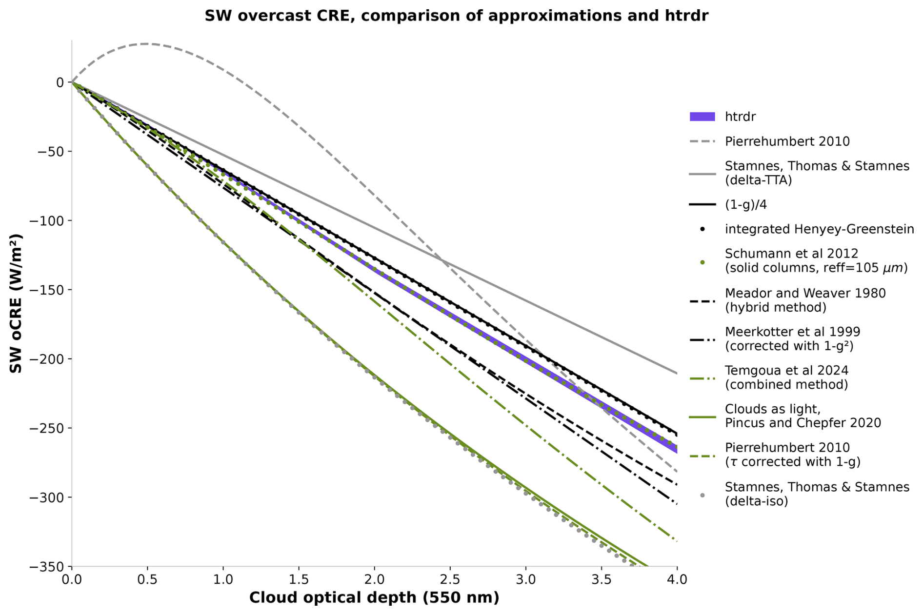
Figure C1 Comparison between SW CRE calculated with htrdr with the independent column approximation (purple) and the different expressions found in the literature listed in Table C2, for the Sun at zenith, as a function of cloud optical depth.

Taking ω₀=1 and g=0.8 (which correspond to optical properties of the ice crystal shapes considered; see Fig. D1 in Appendix D), the Sun at zenith, and the same incoming solar flux at cloud top as htrdr, we obtain the approximated SW CRE as close to htrdr, except for a slightly overestimated slope (Fig. 3a). Figure C1 compares this approximation along with several others found in the literature, most of them showing this quasi-linearity to small optical depths but with very different slopes that do not match htrdr results.

C2 Previously published approximations of SW CRE

As mentioned in Sect. 3.1.1, we tested several approximations of the SW CRE found in the literature. These expressions are plotted in Fig. C1, with comparison to htrdr results. Most expressions are functions of g, ω₀, and τ_c, except for the expression from Schumann et al. (2012), which depends on the effective radius of ice crystals and eight model parameters specific to the ice crystals shape. The values that we use for g and ω₀ are listed in Table C1.

Some approximations can be corrected: Meerkötter et al. (1999) have too strong a slope, which can be corrected by applying a factor (1−g²). Pierrehumbert (2010) works better with a correction (1−g) in term β, i.e., applied to the cloud optical depth in the exponential term. It is interesting to note that Pierrehumbert (2010) specifies that the factor (1−g) should not be applied in the β term, despite the formula fitting better when applying it. The common $(\mathrm{1}-g)/\mathrm{2}$ used in an extensive number of studies in the case of thin clouds differs from htrdr. Surprisingly, the very simple expression $(\mathrm{1}-g)/\mathrm{4}$ is one of the closest to htrdr. However, this might be a coincidence and we cannot conclude that this expression fits in every case.

The Schumann et al. (2012) model does not use the same parameters but fits htrdr remarkably well when used with single columns for the ice crystal shape and an effective ice crystal radius of 100 µm. This is expected, as Schumann's model parameters have been derived from a large set of radiative transfer computations using RT code libRadtran (Mayer and Kylling, 2005) with the DISORT 2.0 solver (Stamnes et al., 1988). The curve labeled “integrated Henyey–Greenstein” in Fig. C1 is obtained by integrating the Henyey–Greenstein scattering phase function over backscattering angles (between $\mathit{\mu }=-\mathrm{1}$ and μ=0). This only works for the Sun at zenith where the upscatter fraction and the backscatter fraction are equal. It is expected to be in good agreement with htrdr since the scattering phase function implemented in the model is Henyey–Greenstein.

Table C1 Parameters used in calculations with the LW and SW CRE expressions listed in Table C2 and shown in Fig. C1.

Meador and Weaver (1980)Schumann et al. (2012)Pierrehumbert (2010)Stamnes et al. (2017)Stamnes et al. (2017)Meerkötter et al. (1999)Temgoua et al. (2024)Siebesma et al. (2020)

Table C2 List of expressions used to calculate cloud reflectivity at zenith in Fig. C1. Values of the parameters common to all expressions are given in Table C1.

Appendix D: Optical properties of ice crystals

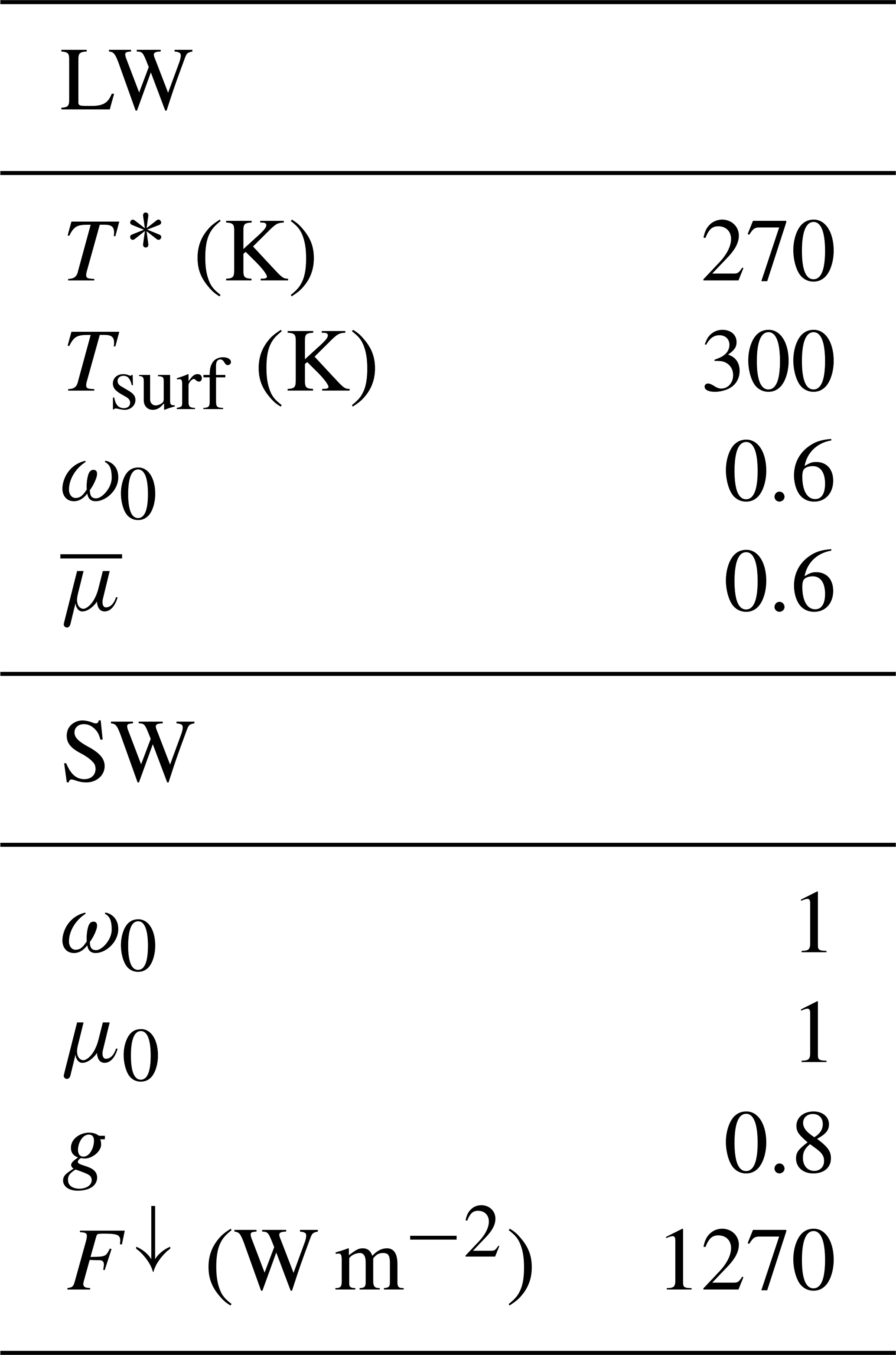
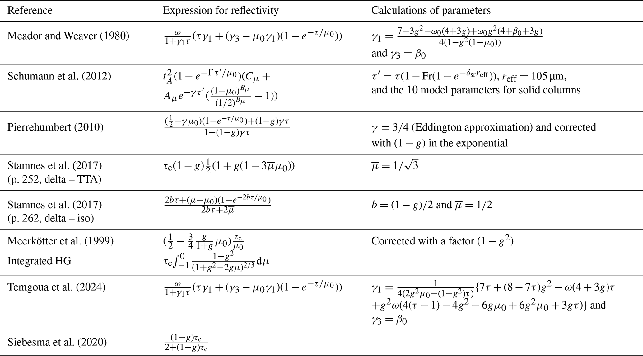
Figure D1 shows the wavelength-dependent asymmetry parameter and single-scattering albedo of ice crystals used for the radiative transfer calculations in this study. It is interesting to calculate their average over the SW and LW spectral domains, weighed by the Planck function at the Sun temperature (T=6000 K) for the SW and cloud temperature (T=229 K) for the LW, represented as dashed lines in Fig. D1. The spectral range of integration is between 0 and 4000 nm in the SW and 4000 and 100 000 nm in the LW. The average values are very close to the ones used in the simple model described in the paper and consistent with values used in other studies for cirrus and contrails (Myhre et al., 2009).

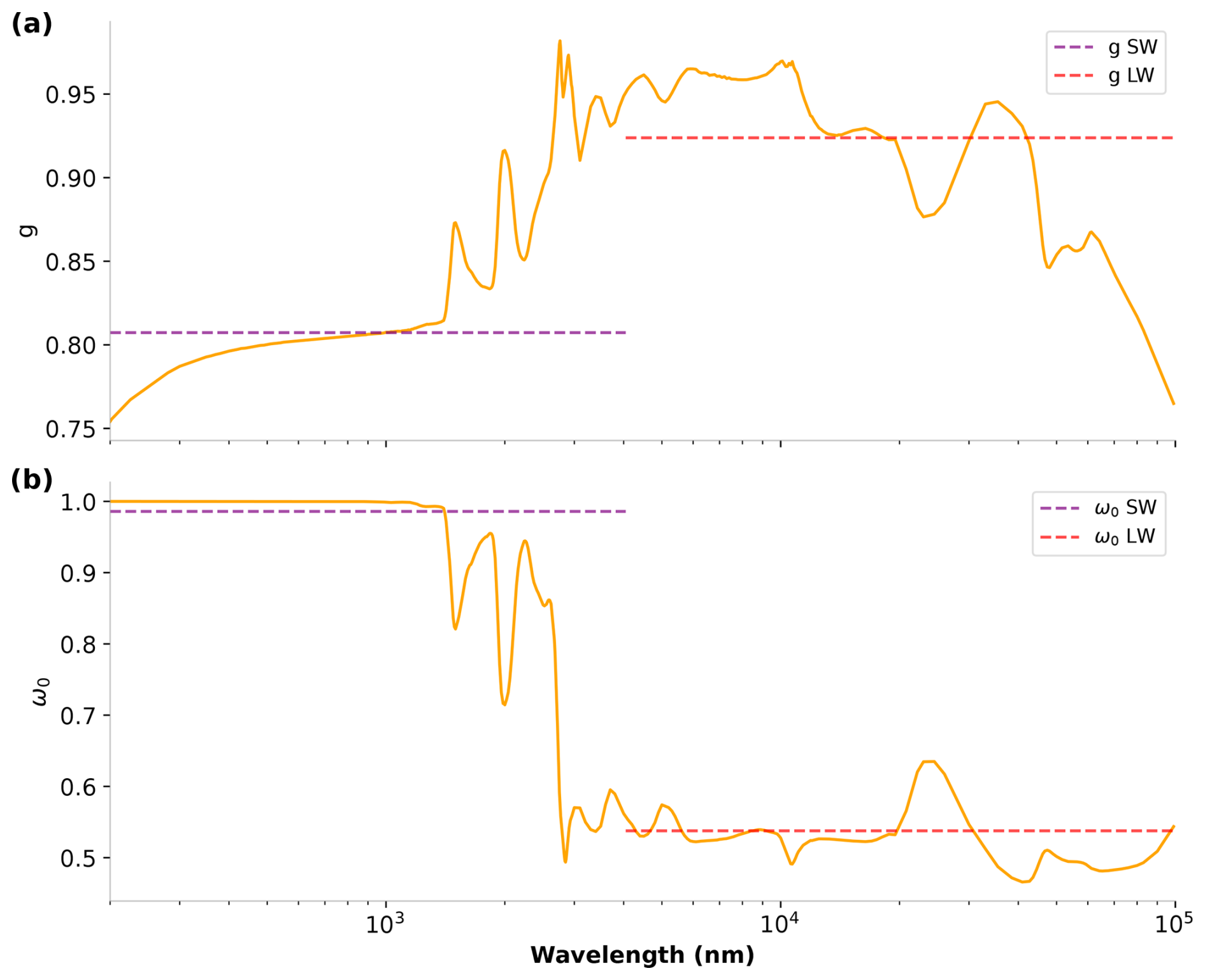
Figure D1 Asymmetry parameter (a) and single-scattering albedo (b) of ice crystals as a function of wavelength and their averages over the SW (purple) and LW (red) spectral domains as dashed lines. Note the log scale on the x axis.

Appendix E: Histograms of solar angles

Figure E1 shows histograms of zenith and azimuth angles for the 3 selected days of the year for 45 and 60° latitude. The figure illustrates the stark contrast in the distribution of solar angles between summer and winter. At 60° latitude in the winter solstice, zenith angles are concentrated in ranges above 80°. Given the challenges associated with calculating fluxes for angles within this range, this subject requires further investigation.

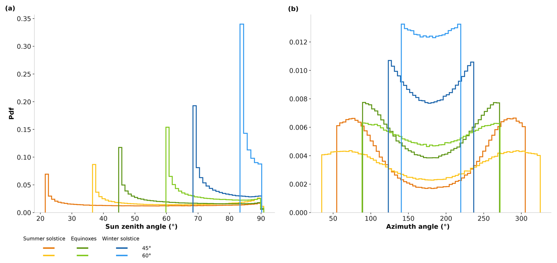
Figure E1 Histogram of Sun zenith (a) and azimuth (b) angles for selected days of the year and latitudes. The displayed angles correspond to the daytime period of the days.