Interannual variability in the Australian carbon cycle over 2015–2019, based on assimilation of Orbiting Carbon Observatory-2 (OCO-2) satellite data

In this study, we employ a regional inverse modelling approach to estimate monthly carbon fluxes over the Australian continent for 2015–2019 using the assimilation of the total column-averaged mole fractions of carbon dioxide from the Orbiting Carbon Observatory-2 (OCO-2, version 9) satellite. Subsequently, we study the carbon cycle variations and relate their fluctuations to anomalies in vegetation productivity and climate drivers. Our 5-year regional carbon flux inversion suggests that Australia was a carbon sink averaging −0.46 ± 0.08 PgC yr⁻¹ (excluding fossil fuel emissions), largely influenced by a strong carbon uptake (−1.04 PgC yr⁻¹) recorded in 2016. Australia's semi-arid ecosystems, such as sparsely vegetated regions (in central Australia) and savanna (in northern Australia), were the main contributors to the carbon uptake in 2016. These regions showed relatively high vegetation productivity, high rainfall, and low temperature in 2016. In contrast to the large carbon sink found in 2016, the large carbon outgassing recorded in 2019 coincides with an unprecedented rainfall deficit and higher-than-average temperatures across Australia. Comparison of the posterior column-averaged CO₂ concentration with Total Carbon Column Observing Network (TCCON) stations and in situ measurements offers limited insight into the fluxes assimilated with OCO-2. However, the lack of these monitoring stations across Australia, mainly over ecosystems such as savanna and areas with sparse vegetation, impedes us from providing strong conclusions. To a certain extent, we found that the flux anomalies across Australia are consistent with the ensemble means of the OCO-2 Model Intercomparison Project (OCO-2 MIP) and FLUXCOM (2015–2018), which estimate an anomalous carbon sink for Australia in 2016 of −1.09 and −0.42 PgC yr⁻¹ respectively. More accurate estimates of OCO-2 retrievals, with the addition of ocean glint data into our system, and a better understanding of the error in the atmospheric transport modelling will yield further insights into the difference in the magnitude of our carbon flux estimates.

1 Introduction

On average, each year, the global terrestrial biosphere absorbs about one-quarter of the total global fossil fuel CO₂ emissions that human activities add to the atmosphere (Friedlingstein et al., 2020). Carbon uptake by the terrestrial biosphere plays an important role in the Earth’s carbon cycle and in future climate projections, as it can slow down the rise in the atmospheric CO₂ concentrations. Due to the uncertainties in quantifying carbon fluxes using terrestrial biosphere models (Sitch et al., 2015), scientists are unsure whether the growth rate of emissions in the atmosphere is going to increase or decrease in the future. In particular, the contributions of semi-arid regional ecosystems, such as those in Australia, are uncertain and are subject to high variability (Trudinger et al., 2016). Identifying and understanding the main drivers behind carbon flux variability in semi-arid ecosystems are crucial processes, not only for understanding the global carbon cycle but also for predicting future trends in atmospheric CO₂ concentration and, consequently, the future of climate change.

Australia's contribution to interannual global carbon cycle variability has been a topic of interest to the carbon cycle research community due to an unusually large land carbon sink anomaly of about −0.70 PgC yr⁻¹ (relative to the 2003–2012 value) recorded in 2011, which alone accounted for 57 % of the global terrestrial carbon uptake anomaly in this period. Poulter et al. (2014) suggested that the reason for this large carbon uptake in Australia was an increase in vegetation cover as the result of increased precipitation in 2011, which was one of the wettest years on record for Australia. Another study performed by Trudinger et al. (2016) found similar results to Poulter et al. (2014); they estimated a carbon uptake anomaly of −0.40 to −0.61 PgC yr⁻¹ (relative to the 1982–2013 value). Global atmospheric inversions based on atmospheric CO₂ concentrations also support this unexpected large sink over Australia. A study carried out by Detmers et al. (2015), based on the assimilation of Greenhouse Gases Observing Satellite (GOSAT) retrievals, found that the carbon sink anomaly in Australia in 2011 was about −0.23 PgC yr⁻¹ (relative to the June 2009–June 2013 period). All of these studies agree that the main driver behind the carbon sink anomaly in 2011 was an increase in the gross primary productivity (GPP) which arose from an increase in rainfall that coincided with a La Niña event that occurred from 2010 to 2011. Haverd et al. (2016) suggested that the carbon sink anomaly recorded in 2011 was 90 % attributable to higher-than-expected carbon uptake by semi-arid ecosystems, such as savanna and sparsely vegetated regions, which was mostly driven by a positive response from these ecoregions to precipitation anomalies.

Ma et al. (2016) suggested that the size of the 2011 carbon sink anomaly in Australia was abruptly reduced in 2012 and then nearly eliminated in 2013 (0.08 PgC yr⁻¹) due to a decrease in rainfall across Australia. In this study, the authors show that productivity in Australia's semi-arid ecosystems is strongly influenced by drivers such as rainfall and temperature. A recent continental-scale inverse modelling study, utilizing Orbiting Carbon Observatory-2 (OCO-2) satellite data, suggests that Australia was a −0.41 ± 0.08 PgC yr⁻¹ sink of CO₂ for 2015 (Villalobos et al., 2021). In this study, the authors indicate that the stronger carbon sink estimated in 2015 was primarily driven by an increase in productivity over savanna and sparsely vegetated regions. Moreover, the authors propose that periods with a stronger carbon uptake were likely related to increased rainfall in Australia's semi-arid ecosystems.

The current study builds upon the work of Villalobos et al. (2021), who only performed an inversion for 2015 and focused on the total mean carbon flux for that period. In this work, we assimilate the total column-averaged retrieval from NASA's OCO-2 to study the interannual variability in the Australia carbon fluxes for the 2015–2019 period. An interesting question that arises is whether the large carbon sink estimated in 2015 over semi-arid ecosystems will follow the same patterns after this year or whether such patterns will become stronger or weaker due to changes in precipitation and temperature.

The paper is organized as follows: Sect. 2 describes the methodology and data that we used to perform the inversion, including a description of the climate drivers and auxiliary data. Section 3 presents the results of our 5-year inversion, including the analysis of the inversion performance, the study of the prior and posterior Australian carbon fluxes, and an assessment of the GPP carbon flux estimate derived from the CABLE model. In this section, we also assess the robustness of the inversion (against independent data) and provide an analysis of the interannual variability in rainfall, temperature, and the enhanced vegetation index (EVI) over semi-arid ecosystems across Australia. Section 4 discusses how well our assimilated OCO-2 carbon fluxes align with other global products – OCO-2 MIP (OCO-2 Model Intercomparison Project) global inversions and FLUXCOM – and gives some directions for future work. Finally, in Sect. 3, we summarize the results of this study.

2 Method and data

We follow the same four-dimensional variational data assimilation approach used to estimate the Australia carbon fluxes described in Villalobos et al. (2021). In this section, we will give a brief description of the system and the data used in the inversion. Further details can be found in Villalobos et al. (2020, 2021).

2.1 Inversion set-up

Our regional inversion system optimizes monthly mean grid-based surface carbon emissions x using a four-dimensional variational data assimilation method that was configured to utilize the Community Multiscale Air Quality (CMAQ, version 5.3) model and its adjoint (version 4.5.1; Hakami et al., 2007). Each year of the 5-year period was run independently, with a spin-up of 1 month for each year. Our system optimizes CO₂ surface fluxes by finding the minimum of the cost function J(x) shown in Eq. (1). Notation in this study follows Rayner et al. (2019).

$$\begin{array}{}\text{(1)}& \begin{array}{rl}J\left(\mathit{x}\right)& ={\displaystyle \frac{\mathrm{1}}{\mathrm{2}}}\left[{\left(\mathit{x}-{\mathit{x}}^{\mathrm{b}}\right)}^T{\mathbf{B}}^{-\mathrm{1}}\left(\mathit{x}-{\mathit{x}}^{\mathrm{b}}\right)\right]\\ & +{\displaystyle \frac{\mathrm{1}}{\mathrm{2}}}\left[{\left(\mathbf{H}\left(\mathit{x}\right)-\mathit{y}\right)}^T{\mathbf{R}}^{-\mathrm{1}}\left(\mathbf{H}\left(\mathit{x}\right)-\mathit{y}\right)\right]\end{array}\end{array}$$

This cost function measures the mismatch between the CMAQ forward model simulation H and OCO-2 satellite observations y as well as the deviation of the control vector x from its background (also termed prior) estimate x^b. In our case, the control vector x (the vector of unknowns) consists not only of the gridded CO₂ surface fluxes but also incorporates initial and boundary conditions (BCs). These two latter variables were incorporated into the control vector to reduce any potential biases related to the boundary inflow that could affect our system (details of how we treat the boundary and initial conditions in our system can be found in Sect. 2.2 in Villalobos et al., 2020, 2021), and a brief description of this treatment is found in Sect. 2.2. R represents the observational error covariance matrix, which was defined as a diagonal matrix (a full description of this covariance matrix is found in Sect. 2.3 in Villalobos et al., 2020), and a brief explanation of how it was constructed is found in Sect. 2.4. B is the associated error covariance matrix of x_b, boundary and initial concentrations, and includes off-diagonal terms. In these off-diagonal values, we only include spatial and non-temporal correlations of the prior fluxes (details of the structure of the prior error covariance matrix are found in Sect. 2.4 in Villalobos et al., 2020), and a summary of its description is found in Sect. 2.3.

The minimization procedure involves iterative calculations of J(x) and its gradient ∇_xJ(x), using the CMAQ forward model H and its adjoint H^T, as shown in Eq. (2):

$$\begin{array}{}\text{(2)}& {\mathrm{\nabla }}_{x}J={\mathbf{B}}^{-\mathrm{1}}\left(\mathit{x}-{\mathit{x}}^{\mathrm{b}}\right)+{\mathbf{H}}^T\left({\mathbf{R}}^{-\mathrm{1}}\left[\mathbf{H}\left(\mathit{x}\right)-\mathit{y}\right]\right).\end{array}$$

The method that our inversion system uses to minimize the J(x) is the limited-memory Broyden–Fletcher–Goldfarb–Shanno (L-BFGS-B) algorithm (Byrd et al., 1995), implemented in the “SciPy” Python module. The L-BFGS-B algorithm iteratively adjusts x until J(x) reaches a minimum. We reached a reasonable convergence for each year run after iteration 25. The ratio between the cost function and the number of observations was close to the theoretical expected value (see details in Sect. 3.1). Posterior uncertainties in this study were assumed to be the same as Villalobos et al. (2020, Sect. 2.4); however, we increase their value by a factor of 1.2 to satisfy the theoretical assumption in the variational optimization (p.211, Tarantola, 1987).

2.2 Initial and boundary conditions

To avoid the effect of initial conditions (ICs) and boundary conditions (BCs) on our OCO-2 assimilated carbon fluxes, we optimized them within the control vector x. Each lateral boundary (south, east, north, and west) of our regional WRF-CMAQ (Weather Research and Forecasting – Community Multiscale Air Quality) model domain was split into two regions. Lateral BCs in the lower layer of the atmosphere were taken from σ=1 to σ=0.96, corresponding (on average) to a pressure of 972.5 hPa, whereas the upper boundary layer was solved from 972.5 up to 50 hPa. Each lateral BC was solved at a monthly scale. Boundary and initial concentrations were taken from CAMS (Copernicus Atmosphere Monitoring Service) global CO₂ atmospheric inversion product data (v19r1) (Frédéric Chevallier, personal communication, 2019). BC uncertainties were assumed to be the standard deviation (1σ uncertainty) in the perimeter of each region of the boundaries, and IC uncertainties were set at 1 % (approximately 4 ppm). A diagram of the WRF-CMAQ domain is illustrated in Fig. 1.

Figure 1 The horizontal WRF-CMAQ modelling domain (shown using lighter colours) based on the Lambert conformal projection.

2.3 Transport model and prior fluxes

The CMAQ model was used to simulate atmospheric transport and dispersion. These simulations, which were run offline from the meteorological model, were conducted without atmospheric chemistry. The meteorological data used as input for the CMAQ model were taken from the WRF model, version 4.1.1 (Skamarock et al., 2008). We run the CMAQ model at an hourly resolution at a grid cell scale of 81 km. The model has 32 vertical levels using the terrain-following σ vertical coordinate system. Details of the parameterizations are listed in Villalobos et al. (2021, Sect. 2.4, Table 1). We run WRF at a spatial resolution of 81 km on a single domain (i.e. non-nested). WRF initial conditions were taken from the ERA-Interim global atmospheric reanalysis (Dee et al., 2011), which has a resolution of approximately 80 km on 60 vertical levels from the surface up to 0.1 hPa. Sea surface temperatures were obtained from the National Centers for Environmental Prediction/Marine Modeling and Analysis Branch (NCEP/MMAB). The WRF model was run with a spin-up period of 12 h.

The prior flux estimates used in our inversion consisted of four datasets: land–biosphere fluxes, fossil fuel, fires, and ocean fluxes. Biosphere carbon fluxes were simulated by the Community Atmosphere Biosphere Land Exchange (CABLE) model set up in the BIOS3 modelling environment, a fine resolution offline environment built on capability developed for the Australian Water Availability Project (AWAP) (King et al., 2009), hereafter referred to as CABLE BIOS3 (Haverd et al., 2018). The CABLE land surface model consists of a biophysical core: a biogeochemical module including a nitrogen and phosphorous cycle (Wang et al., 2010), the “Populations-Order-Physiology” (POP) module for woody demography and disturbance-mediated landscape heterogeneity (Haverd et al., 2013b), and a module for land use and land management (POPLUC; Haverd et al., 2018). However, the functionality of POPLUC was not considered in BIOS runs, and the land use change remained static at the year 2000. CABLE can be run at global or regional scales. For our regional study case, CABLE was run at a regional scale (resolution 0.25^∘), and it was forced with Australian regional drivers and observations (BIOS3 set-up). Biosphere fluxes from CABLE (roughly net biome productivity – NBP) include gross primary productivity (GPP) and net ecosystem respiration (autotrophic and heterotrophic respiration); however, they do not include carbon losses from fire disturbances, harvest, erosion, and export of carbon in river flow. We used the averages of 3-hourly NBP estimates as input for CMAQ (further details of how we constructed NBP can be found in Sect. 2.3 in Villalobos et al., 2021). The prior error covariance matrix of the terrestrial biosphere flux from CABLE was assumed to be an approximation of the net primary productivity (NPP), following the approach of Chevallier et al. (2010), with a ceiling of 3 gC m⁻² d⁻¹. We assumed that these uncertainties were spatially correlated with length scale of 500 km over land, following Basu et al. (2013). Within our inversion system, no temporal correlations were considered.

Fossil fuel emissions used here were based on two different inventory datasets: the Open-source Data Inventory for Anthropogenic CO₂ (ODIAC, version 2019; Oda et al., 2018) and the Emissions Database for Global Atmospheric Research (EDGAR; Crippa et al., 2020). We added some missing sectors from the EDGAR inventory to ODIAC (such as aviation climbing and descent, aviation cruise, and aviation landing and take-off datasets). ODIAC is a global gridded product distributed at a 0.1^∘ × 0.1^∘ spatial resolution over land that uses power plant profiles (emission intensity and geographical location) and satellite-observed night-time lights. We used ODIAC monthly fluxes and incorporated a diurnal scale factor to estimate diurnal CO₂ emission variability (Nassar et al., 2013). Given that the ODIAC product only covers the period from 2015 to 2018, we repeated the data from 2018 in 2019 but increased the value in each grid cell by 1.7 %, which represents the mean annual growth rate of these emissions from 1970 to 2018. EDGAR is also gridded at 0.1^∘ × 0.1^∘ with a monthly temporal resolution. There is no EDGAR gridded product for 2016–2019, so we repeated the 2015 product to cover the other years. We increased EDGAR aviation emissions by 2.5 %, which represents the mean growth rate in this emissions sector from 2016 to 2019. Fossil fuel prior uncertainties were assigned to be 0.44 times the value of the monthly fossil fuel estimates described above (see details in Sect. 2.3 in Villalobos et al., 2021). Errors in fossil fuel emissions were assumed to be uncorrelated.

Ocean flux estimates were selected from CAMS global data (v19r1) (Frédéric Chevallier, personal communication, 2019). Ocean prior uncertainties were assumed to be 0.2 gC m⁻² d⁻¹ and uniform across the ocean, as in Chevallier et al. (2010). Similar to correlations for biosphere prior uncertainties, uncertainties in ocean fluxes were assumed to be correlated in space with a length scale of 1000 km. Fire prior emissions were selected from the Global Fire Emissions Database (GFED, version 4.1s), which includes emissions from small fires. Fire emission uncertainties were assumed to be 20 % of the GFED emissions and correlated in space with a length scale of 500 km, but they were not assumed to be correlated in time. The combination of all prior fluxes was regridded to the spatial resolution of the CMAQ model.

2.4 OCO-2 observations and their uncertainties

Our regional inversion assimilates satellite observations derived from NASA's Orbiting Carbon Observatory-2 (OCO-2; Eldering, 2018). The OCO-2 satellite instrument carries a single instrument that incorporates three-channel imaging grating spectrometers developed to measure sunlight reflected by the Earth's surface in three spectral bands: two CO₂ spectral bands in the short-wave infrared (SWIR) at 1.6 and 2.1 µm respectively and one in the near-infrared (NIR) at 0.76 µm (O₂ A-band). From these radiance spectra, it is possible to calculate the column-averaged dry-air mixing ratio of carbon dioxide. The OCO-2 employs three different sampling strategies to collect data: nadir mode, glint mode, and target mode. Nadir observations provide useful information over land because the satellite points straight down at the surface of the Earth (surface solar zenith angle is less than 85^∘). In glint mode, the instrument points to the bright glint spot on Earth where solar radiation is directly reflected off the Earth's surface (local solar zenith angle is less than 75^∘). In target mode, the instrument points towards a specific location on the ground. Target mode is use for validation, where the performance of the instrument is validated against ground-based observations from the Total Carbon Column Observation Network (TCCON) (Wunch et al., 2011).

In this study, the regional inversion was performed using a combination of both land (nadir and glint – LNLG) OCO-2 observations (version 9). We used the combination of both datasets, as Miller and Michalak (2020) demonstrated that combining both modes provides a stronger and better constraint on CO₂ fluxes at regional scales. Moreover, both datasets present negligible bias (O'Dell et al., 2018). We did not incorporate ocean glint measurements in our inversion, as ocean observations still have undetermined biases (O'Dell et al., 2018) that might impact the Australian carbon flux estimates.

OCO-2 LNLG data from December 2014 to December 2019 were selected. We considered OCO-2 data from December 2014, as we ran CMAQ with a spin-up of 1 extra month. As an example, Fig. E1 in the Appendix shows the spatial pattern of OCO-2 soundings (LNLG) that fall in our CMAQ domain for 2015. In this figure, we can see that OCO-2 data provide a very good coverage of the Australian region. Such spatial coverage offers good potential to help constrain regional biosphere CO₂ fluxes.

Given that the OCO-2 spatial resolution (1.29 km × 2.25 km) is higher than the CMAQ model grid cell resolution (81 km × 81 km), the OCO-2 data were averaged to the CMAQ model grid level following the two-step process described in Villalobos et al. (Sect 2.3, 2021): the first step involves averaging all OCO-2 soundings across 1 s intervals, while the second step involves averaging these 1 s averages into the CMAQ vertical column (approximately 11 s averages). The algorithm to estimate the uncertainties across 1 s averages follows Crowell et al. (2019). Here, we considered three different forms of uncertainty calculation. First, we assumed that uncertainties that fall within a 1 s span were perfectly correlated in time and space (uncertainties defined as σ_s). Second, given that the average of OCO-2 uncertainties (σ_s) is relatively low compared with the real OCO-2 uncertainties (mainly because they only consider the errors from measurement noise and are not systematic errors), we also used the spread (standard deviation) of the OCO-2 retrievals in the 1 s average (uncertainties defined as σ_r). Third, we also considered a baseline uncertainty (defined as σ_b) for cases where the number of OCO-2 soundings was not high enough to compute a realistic spread. Our baseline uncertainties were assumed to be 0.8 ppm over land and 0.5 ppm over ocean. Finally, we selected the maximum value between these three uncertainties (σ_s, σ_r, and σ_b). For each grid cell, we also added (in quadrature) 0.5 ppm to this term as the contribution of the CMAQ model uncertainty (defined as σ_m). We also increased the final observation uncertainty by a factor of 1.2 to satisfy the theoretical assumptions of the inversion (Villalobos et al., 2021). We interpolated the retrieval OCO-2 profile to the CMAQ model vertical profile as described in Villalobos et al. (2020, Sect. 2.6). Note that we only selected bias-corrected data and OCO-2 retrievals with a quality flag of “0”, as described by Kiel et al. (2019).

2.5 Validation data

2.5.1 TCCON

For validation of our inversion, we compared our posterior column-averaged concentration simulated by CMAQ with the TCCON sites located in Australia and New Zealand (Fig. 2). TCCON is a network of ground-based Fourier transform spectrometers (FTSs) recording direct solar spectra in the NIR and SWIR spectral regions (Wunch et al., 2011). From these spectra, accurate and precise total column amounts of CO₂ and other trace gases are retrieved. In our study domain, there are three TCCON stations (Darwin, Wollongong, and Lauder). The Darwin and Wollongong sites are located within Australia, whereas the Lauder site is located in New Zealand. The Darwin and Wollongong sites are operated by the Centre for Atmospheric Chemistry at the University of Wollongong, Australia (Griffith et al., 2017a, b). The Lauder site is operated by New Zealand's National Institute of Water and Atmospheric Research (NIWA) (Sherlock et al., 2017; Pollard et al., 2019). As is shown in Fig. 2, the Lauder monitoring station is located on the South Island of New Zealand, 2 km north of the town of Lauder; it is sheltered from the prevailing wind direction by the Southern Alps, which increases the number of days with clear skies and results in an air mass that is largely unmodified by regional anthropogenic sources (Pollard et al., 2017). Since mid-2015, the Darwin site has been located about 9 km east of Darwin city, approximately 4.5 km south-east of its previous location (Deutscher et al., 2010). The Wollongong site is a coastal site that is close to populated areas and industry to the north and close to native forest and less densely populated areas to the south and west (Deutscher et al., 2014). At each site, TCCON data were selected within 1 h windows and averaged to be consistent with the temporal resolution of the output of the CMAQ simulations. Each TCCON retrieval is provided with an averaging kernel and a prior profile, which were interpolated to the CMAQ vertical profiles. After the interpolation, we applied the averaging kernel (following Eq. 15 in Connor et al., 2008) to compute the TCCON CMAQ simulated CO₂ concentrations. The residual between CMAQ and TCCON was constructed based on monthly mean concentrations, which were calculated by taking local time averages between 10:00 and 14:00 LT, when the solar radiation intensity is most stable (Kawasaki et al., 2012).

2.5.2 Ground-based in situ measurements

We also compared our posterior concentrations against four ground-based in situ monitoring sites: Cape Grim, Gunn Point, Burncluith, and Ironbark, whose geographic locations are shown in Fig. 2. These monitoring sites form part of the Global Atmosphere Watch (GAW) programme of the World Meteorological Organization (WMO), and they are operated by the Climate Science Centre of the Commonwealth Scientific and Industrial Research Organisation (CSIRO), located in Aspendale, Australia. We used hourly data from these monitoring sites, but the monthly mean averaged data shown in Sect. 3.4.2 were calculated using local time averages (12:00–05:00 LT, Australian local time, with respect to the monitoring site locations).

Atmospheric CO₂ concentration measurements at the Gunn Point, Ironbark, and Burncluith sites are made continuously at high frequency (∼ 0.3 Hz) using Picarro cavity ring-down spectrometers. Instruments located at the Gunn Point and Ironbark sites are the Picarro model G2301, whereas the Burncluith site uses the Picarro model G2401. All of the inlets are placed at a height of 10 m. Descriptions of the Ironbark, Gunn Point, and Burncluith installations can be found in Etheridge et al. (2016). Cape Grim also operates a Picarro G2301 analyser; however, the inlet is positioned at 70 m. The instrument precision for these spectrometers is better than 0.1 ppm (Etheridge et al., 2014), and all measurements are calibrated to the WMO CO₂ X2007 mole fraction scale (Zhao and Tans, 2006), ensuring comparability between all measurements used. We note that we used “baseline” and “non-baseline” data from Cape Grim. Baseline data are selected when winds blow straight off the Southern Ocean and have not been in recent contact with land. In this study, we used both datasets because our inversion only uses OCO-2 soundings located over land.

Figure 2 Location of the Total Carbon Column Observing Network (TCCON) sites across Australia and New Zealand (red points) and in situ sites (blue points). This map also shows a classification of six bioclimatic regions for Australia.

2.6 Australian bioclimatic classification

To understand which ecosystems contributed the most to the Australian interannual carbon flux variability between 2015 and 2019, we divided the continent into six bioclimatic classes: tropics, savanna, warm temperate, cool temperate, Mediterranean, and sparsely vegetated (Fig. 2). We used the same six bioclimatic regions at a 0.05^∘ spatial resolution as in Haverd et al. (2013a). The classes were regridded over our CMAQ grid (81 km × 81 km) resolution.

2.7 Climate data

In order to analyse the impact of climatic drivers on Australian terrestrial carbon cycle variability, we investigated the anomalies of rainfall and temperature across Australia for the 2015–2019 period. Rainfall data were selected from the Australian Water Availability Project (AWAP), Bureau of Meteorology (BOM) (Jones et al., 2009), for the 2015–2019 period. AWAP is a gridded product at a 0.05^∘ resolution. It is generated by spline interpolation of in situ rainfall observations. We also used air temperature data at 2 m above the land surface from ERA5, the fifth generation of European Centre for Medium-Range Weather Forecasts (ECMWF) atmospheric reanalyses. The dataset selected from ERA5 was monthly and was gridded at a 0.25^∘ spatial resolution. We constructed 3-month running means of rainfall anomalies and air temperature anomalies relative to a mean across 2015–2019. These anomalies were calculated by subtracting their long-term mean (2015–2019) for each month from the raw time series and constructing the 3-month running mean on the resultant time series. We regridded the rainfall anomalies onto the grid of the CMAQ model in order to simplify the comparison with the estimated terrestrial carbon uptake from the flux inversions.

2.8 The enhanced vegetation index (EVI) as an indicator of the vegetation greenness

Plant photosynthesis and respiration are two fundamental physiological processes in the carbon cycle. Physiological and structural changes in vegetation modulate the exchange of CO₂ between the land and atmosphere. In order to understand what physiological factors drive the interannual variability in our posterior fluxes, we studied the anomalies of the enhanced vegetation index (EVI). The EVI provides information on vegetation state, and we used it to characterize changes in Australian vegetation greenness and activity (e.g photosynthesis) from 2015 to 2019. The EVI product was derived from the Moderate Resolution Imaging Spectroradiometer (MODIS) – which flies on board Terra, a NASA Earth-observing satellite (Didan, 2014) – MOD13C1 Version 6 data product. The MODIS EVI is a gridded product that has a 16 d composite temporal resolution and a 0.05^∘ spatial resolution. The EVI ranges from −0.2 to +1, where values less than 0 indicate a lack of green vegetation or arid areas. We calculate the 3-month running mean of EVI anomalies in Australia relative to the long-term mean from 2015 to 2019 and subtract the mean seasonal cycle. These monthly EVI MODIS products were also regridded into the CMAQ domain to calculate the temporal correlation between prior and posterior flux anomalies.

2.9 Gross primary productivity (GPP)

To understand the difference between posterior and prior fluxes, we compared the climatological seasonal cycle of the gross primary productivity (GPP) from the CABLE BIOS3 model against the remote-sensing-based DIFFUSE model (Donohue et al., 2014) and against the latest MODIS Terra GPP product (MOD17A2H Version 6) (Running et al., 2015) for the 2015–2019 period. We also calculated the 3-month running mean GPP anomalies for these three datasets.

The DIFFUSE GPP estimates are taken to be the product of the fraction of photosynthetically active radiation (PAR) absorbed by vegetation and the light use efficiency. These datasets have a temporal resolution of 16 d at a 250 m spatial resolution. Similar to the DIFFUSE estimates, the MODIS GPP product is based on a light use efficiency approach and provides a cumulative 8 d composite product gridded at 500 m. For comparison, the CABLE BIOS3, DIFFUSE, and MODIS GPP products were averaged to a monthly resolution and regridded over the CMAQ domain.

2.10 Global atmospheric inversions

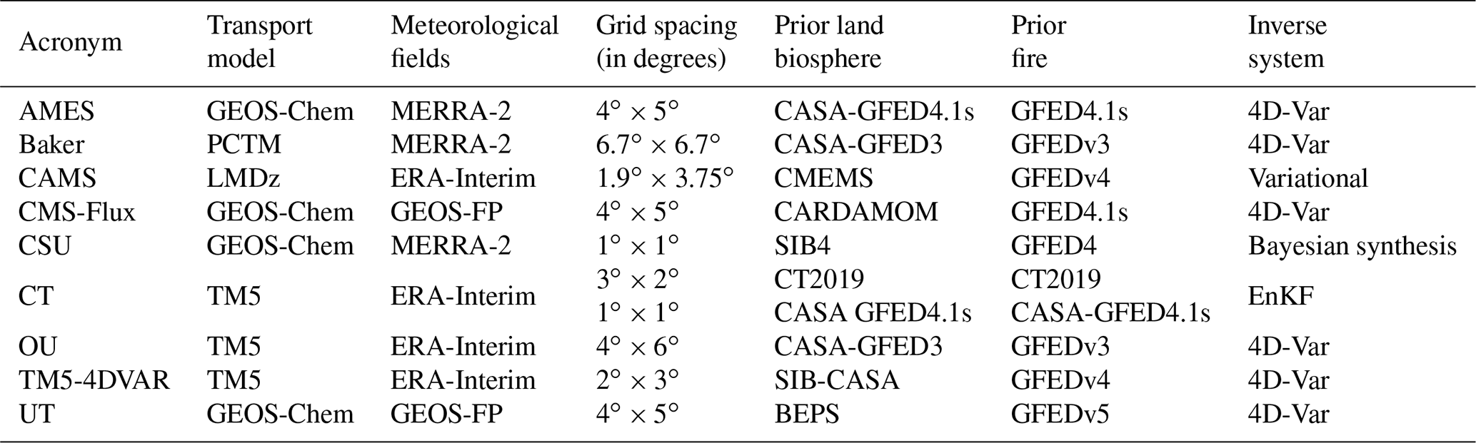
We compared our Australian assimilated fluxes against nine independent global atmospheric inversions: AMES, PCTM, CAMS, CMS-Flux, CSU, CT, OU, TM5-4DVAR, and UT (Sect. 4). These global inversions are part of the OCO-2 Model Intercomparison Project (OCO-2 MIP) (Crowell et al., 2019; Peiro et al., 2022). In this study, we used the OCO-2 MIP flux version found in Peiro et al. (2022). In Peiro et al. (2022), the global inversions were performed using the assimilation of OCO-2 data (version 9, bias corrected) from 2015 to 2018. A summary of these nine global inversions is given in Table 1, and a complete description of them and their input fields can be found in Peiro et al. (2022, Appendix A: model information). We can see from Table 1 that all global inversions were run using different inverse systems and were configured at different spatial resolutions with different atmospheric transport models and prior fluxes. Some global inversion methods use a four-dimensional variational (4D-Var) approach, whereas others utilize a technique known as ensemble Kalman filter (EnKF) or Bayesian synthesis.

Table 1 Summary of the configuration of the OCO-2 MIP (version 9) design.

2.11 FLUXCOM carbon fluxes

We also compared our assimilated fluxes against the FLUXCOM net ecosystem exchange (NEE) ensemble mean product. The FLUXCOM dataset is created using machine learning approaches, which combine data from FLUXNET eddy covariance towers (site-level observations) with satellite remote sensing, and meteorological data to estimate carbon fluxes, such as NEE, along with their uncertainties (Jung et al., 2020; Tramontana et al., 2016). For this study, we downloaded the products at a monthly temporal resolution from the data portal of the Max Planck Institute for Biogeochemistry (https://www.bgc-jena.mpg.de, last access: 6 April 2022).

3 Results

3.1 Inversion performance

In our inversion system, the L-BFGS-B algorithm iteratively adjusts the control vector until the cost function reaches an optimal solution. In Bayesian inverse problems, we require that the observational residuals (simulated – observed) and increments (posterior – background) are consistent with the assumed probability density functions (PDFs). This implies that the cost function should be approximately half the number of observations (Tarantola, 1987, p. 211). Table 2 shows the analysis of convergence for our 5-year inversion. In this table, we can see that, for each year, the ratio between final cost function J(x) and observation was about 0.5, indicating that our system is self-consistent.

Table 2 Convergence diagnostics of the inversion system using OCO-2 satellite data.

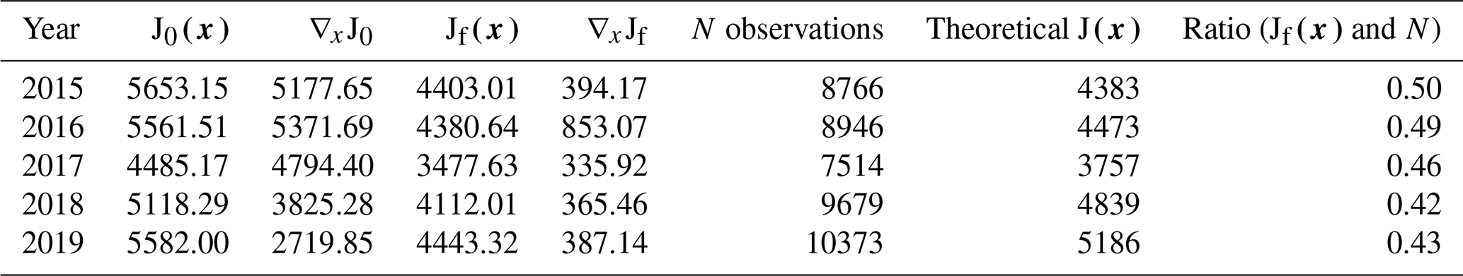
Figure 3 shows the monthly bias and the root-mean-square error (RMSE) between the prior and posterior column-integrated concentrations simulated by CMAQ against the OCO-2 observations. In this figure, we can see that the inversion generally reduces prior biases significantly to values close to zero. As an indication of the overall inversion performance, the Australian mean prior bias for 2015–2019 was reduced from 0.23 to 0.06 ppm and the RMSE was reduced from 0.90 to 0.76 ppm (Fig. A1).

While we see that inversion reduces the prior biases significantly, relatively small positive systematical posterior biases remain (0.05 ppm). These systematic positive posterior biases across Australia are likely driven by sampling and residual retrieval biases in the OCO-2 data. Some studies suggest that the existing OCO-2 cloud-screening algorithm (Taylor et al., 2016) has difficulty identifying clouds near the surface (shallow-layer clouds). Unresolved low-level clouds introduce significant biases in the retrieved column of CO₂ concentration.

We note that the data gap in August and September was caused by a satellite outage. In November 2017, we observed that the prior concentration underestimated the observations significantly, with biases of about −0.56 ppm and an RMSE of 1.29 ppm. High prior biases in this month were found along the east coast of Australia, suggesting that the CABLE model might likely be underestimating the carbon outgassing in this area and, therefore, the prior retrieval column CO₂ concentration. The reduction of the prior biases in this month was about 90 % (−0.06 ppm with an RMSE of 0.94).

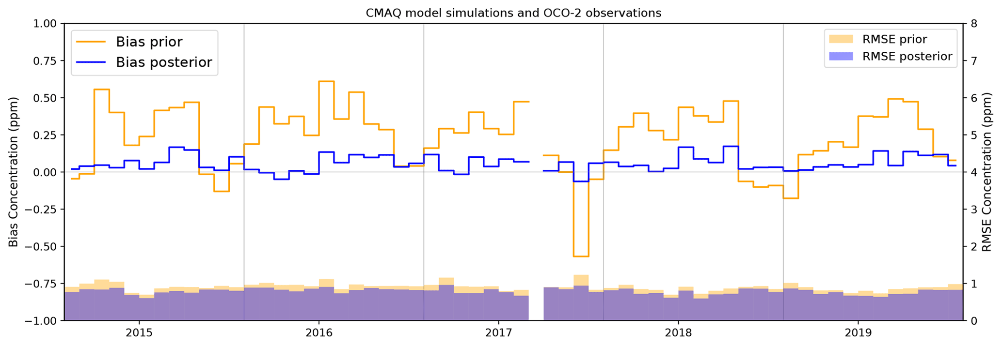
Figure 3 Bias and root-mean-square error (RMSE) between OCO-2 and the prior and posterior concentrations simulated by the CMAQ model. The respective orange and blue lines represent prior and posterior concentration biases, and the respective orange and purple shaded areas represent the prior and posterior RMSE.

3.2 Seasonal cycle and spatial distribution of the Australian prior and posterior carbon fluxes

Before assessing the interannual variability in the fluxes derived by the assimilation of OCO-2 observations, we first examine the monthly, seasonal, and annual means between the prior and posterior fluxes. This step is relevant for the subsequent evaluation of how well the posterior column-averaged concentrations simulated by the CMAQ model fit with independent data. Assessing the robustness of our inversion with independent data will allow us to better explain the posterior flux anomalies derived by our inversion.

Figure 4a shows the long-term mean of the prior and posterior carbon fluxes aggregated across Australia for the 2015–2019 period, and Figs. 4b and c show the annual and seasonal cycle of these estimates. Posterior flux uncertainties from 2016 to 2019 were assumed to be the same as those calculated for 2015, which were estimated by five different observing system simulation experiments (OSSEs; see more details in Villalobos et al., 2021).

Our 5-year inversion suggests that Australia was a carbon sink of −0.46 ± 0.09 PgC yr⁻¹, compared with the prior flux estimate of 0.11 ± 0.17 PgC yr⁻¹ (Fig. 4a). Here, the prior flux estimate (fluxes derived by the CABLE model) represents the current knowledge of the Australian carbon budget. Due to the size of the uncertainties in the prior estimate, it cannot be concluded with high confidence whether Australia was a sink or source of CO₂ for the 2015–2019 period. The annual posterior fluxes also suggest that Australia's terrestrial biosphere is able to absorb more carbon from the atmosphere than the CABLE model estimate (Fig. 4b). Moreover, we see that 2016 was the year that contributed most to the long-term mean sink estimated by the OCO-2 inversion.

In terms of a seasonal cycle, we can see that the posterior flux estimates show a stronger seasonality compared with the prior flux estimate (Fig. 4c). Over the 5 years from 2015 to 2019, we observe that OCO-2 sees a strong seasonal biospheric carbon uptake each year between June and September (winter and early spring in Australia) as well as a stronger carbon source from November to December (late spring and early summer in Australia). As we showed in Fig. 3, the stronger carbon uptake seen in winter and early spring occurs because the prior column-averaged concentration simulated by CMAQ model overestimates OCO-2 observations during this period.

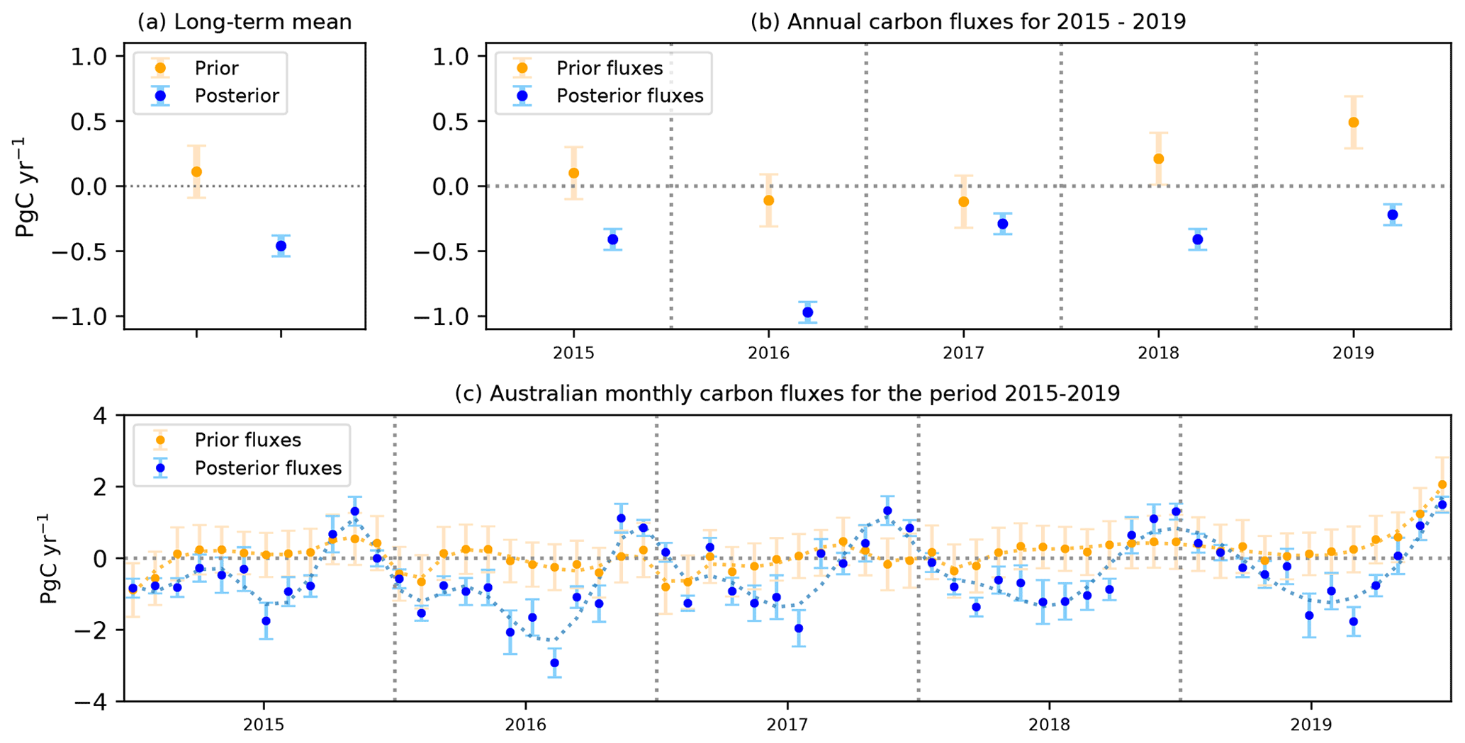
Figure 4 (a) Long-term mean carbon flux, (b) annual mean carbon flux, and (c) monthly mean prior (orange dots) and posterior (blue dots) carbon fluxes as well as their uncertainties (in PgC yr⁻¹) over Australia for the 2015–2019 period. Uncertainties in the prior and posterior fluxes are indicated by bars. The dashed orange and blue lines represent a smooth line for the prior and posterior fluxes respectively. Within these estimates, we only included the terrestrial part of the Australian carbon cycle, including fires but not fossil fuel emissions.

To identify the Australian regions in which the OCO-2 satellite sees a stronger carbon uptake, we plotted the annual difference between the posterior and the prior fluxes (Fig. 5). In Fig. 5a, we see that the majority of the posterior long-term mean flux for the 2015–2019 period is distributed in one half of the continent (in the north-east, central, and southern regions of the continent). However, we note that this was not the case for the coastal region in these areas, where we observe that OCO-2 recorded a stronger carbon release compared with the prior estimate.

The substantial difference between the prior and posterior flux in 2015 and 2016 comes from the northern and south-eastern regions of Australia (excluding coastal areas in the south-east of the continent). In Sect. 3.5, we show that the stronger carbon uptake recorded by the inversion (relative to the prior) in these 2 years was driven by an increase in vegetation productivity due to a rise in rainfall and lower temperatures across these regions. Despite the fact that 2016 was one of the strongest El Niño events on record in the Pacific Ocean, the rain over Australia was above average for most of the continent. The annual climate report from the Bureau of Meteorology for 2016 indicates that the annual rainfall over Australia was 17 % above the 1961–1990 average. In 2017, prior and posterior differences were seen in the northern, central, and eastern coastal areas of Australia. Rainfall in 2017 was below average for much of eastern Australia and along the west coast of Australia. For 2019, OCO-2 recorded a stronger carbon release in western and central Australia. These results are not unexpected, as 2019 was an exceptional year (the hottest and driest year on record in Australia) with a mean temperature that was 1.52 ^∘C above the 1961–1990 average (Annual climate statement, Bureau of Meteorology, 2019). We also noticed a large carbon uptake (relative to prior) in the south-eastern corner of Australia in 2019 (Fig. 5f).

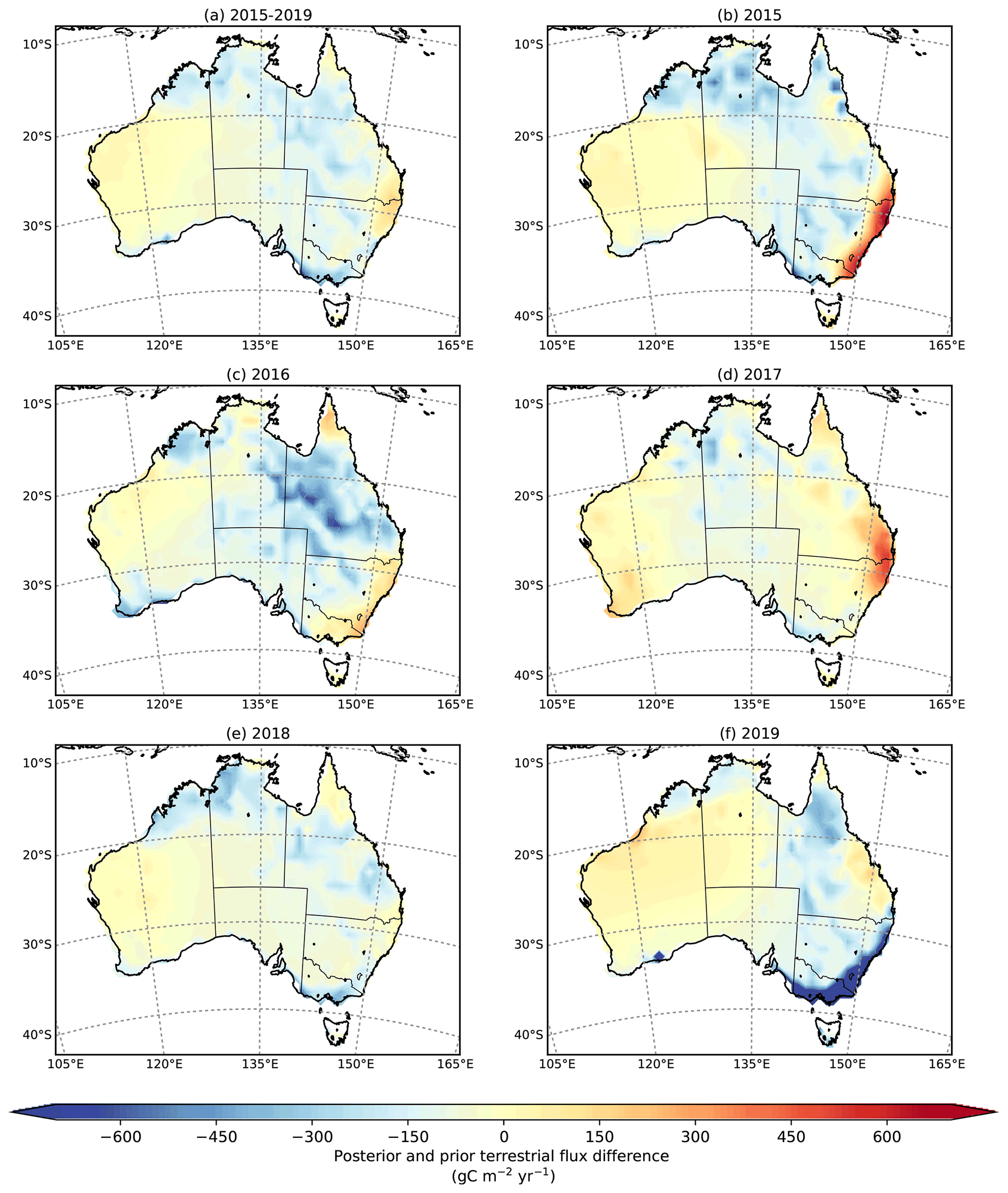
Figure 5 Annual spatial pattern of the differences between posterior and prior carbon fluxes for 2015–2019 (gC m⁻² yr⁻¹).

3.3 Climatological seasonal cycle of the prior and posterior carbon fluxes aggregated by bioclimatic region

To further examine what might potentially be the cause of the difference between the posterior and prior fluxes described above, we compared the climatological seasonal cycle (Fig. 6) against the climatological seasonal cycle of the gross primary productivity (GPP) fluxes derived from CABLE BIOS3, MODIS, and the DIFFUSE model (Fig. C1). We made this comparison by aggregating the fluxes over six bioclimatic regions.

It is evident that the largest difference between prior and posterior flux estimates is over savanna (Fig. 6b) and sparsely vegetated (Fig. 6d) ecosystems. Over the savanna region, the most notable difference is seen from June to September. The absolute difference in this period is about 0.4 to 0.5 PgC yr⁻¹. According to MODIS and DIFFUSE GPP estimates, the stronger posterior sink observed in this period may be due to an underestimation of GPP simulated by the CABLE BIOS3 model (Fig. C1b). The GPP estimated by MODIS from June to September was about 0.90 PgC yr⁻¹ compared with the CABLE BIOS3 estimate of 0.59 PgC yr⁻¹. DIFFUSE GPP estimates were around 0.68 PgC yr⁻¹.

Over the sparsely vegetated region, the seasonal discrepancy between the prior and posterior flux is more evident than for savanna. The seasonality of the posterior flux is stronger (relative to the prior estimate) from April to September. In this ecosystem, the largest absolute difference between the prior and posterior fluxes is seen from June to August (0.5 PgC yr⁻¹). In July, for example, the inversion shifts the prior flux from −0.05 ± 0.09 to −0.56 ± 0.06 PgC yr⁻¹. Again, in Fig. 6d, we can see that a possible reason of this shift may be associated with an underestimation of the GPP by CABLE BIOS3. It is evident that MODIS and DIFFUSE GPP have a stronger seasonality than CABLE BIOS3 GPP. For example, from June to August, the CABLE BIOS-3 GPP was about 0.4 PgC yr⁻¹ compared with DIFFUSE and MODIS, which were 0.9 and 1.3 PgC yr⁻¹ respectively. We did not find a seasonal correlation between the prior fluxes and MODIS and DIFFUSE GPP fluxes (Table G1), but we did find a positive correlation between the posterior fluxes and the GPP estimated by MODIS and DIFFUSE (R=0.44 and R=0.45 respectively).

Regarding the tropical, warm temperate, cool temperate, and Mediterranean ecosystems, the seasonal correlations with the MODIS or DIFFUSE GPP estimates were stronger for the prior than for the posterior fluxes (Table G1). A stronger correlation between the prior flux and MODIS and DIFFUSE might be attributable to the fact that the assimilated coastal fluxes might somehow be less constrained by the inversion in these ecosystems, mainly because they are mostly influenced by ocean fluxes where the uncertainties have less freedom to be modified by the inversion.

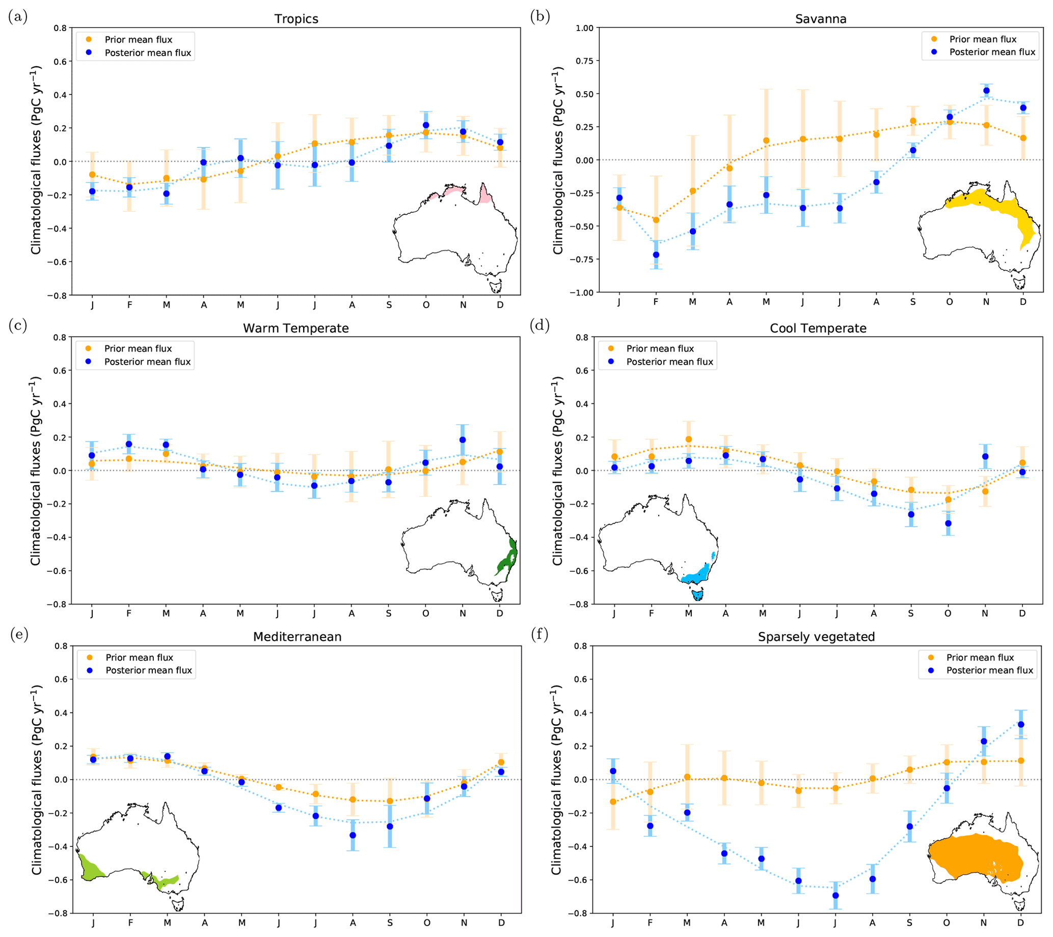
Figure 6 Climatological seasonal cycle of prior (orange points) and posterior (blue points) terrestrial carbon fluxes (2015–2019). The dashed orange and blue lines represent a smooth line for the prior and posterior fluxes respectively.

3.4 Evaluation of the inversion against independent data

To evaluate the accuracy of the posterior fluxes discussed in the previous section, we assess the fit between the posterior concentration CO₂ field (derived by running the CMAQ model with the fluxes assimilated by OCO-2) and independent CO₂ measurements: TCCON (Darwin, Wollongong, and Lauder) and in situ measurements (Gunn Point, Ironbark, Burncluith, and Cape Grim).

3.4.1 Comparison with TCCON data

Figure 7a, c, and e show the time series of the monthly mean column-averaged CO₂ concentrations at the TCCON sites (Darwin, Wollongong, and Lauder) compared to the column-average concentrations from the prior and posterior simulated by CMAQ for 2015–2019. Figure 7b, d, and f show the bias and root-mean-square error (RMSE) from these averages. Monthly averages were computed using data selected between 10:00 and 14:00 LT (Australia or New Zealand local time with respect to the site location).

For all TCCON sites, we found that assimilating OCO-2 data only slightly reduced the prior bias and RMSE. At the Darwin site (Fig. 7a), the fit between the posterior column-averaged concentration and TCCON notoriously degraded at the beginning of 2017, 2018, and 2019 (mainly February and March). High negative posterior biases (2 ppm) may be related to the small number of OCO-2 soundings located around the site or local biases in the OCO-2 data (Peiro et al., 2022). The small number of OCO-2 observations around Darwin is due to the presence of cloud cover and aerosols. While northern Australia experiences a wet season in summer (November to April), which is highly impacted by monsoonal rains and storms, winter (the dry season in this region) is affected by fires. Some studies (e.g. Taylor et al., 2016) suggest that some OCO-2 retrievals can be biased by clouds during the wet season and by smoke aerosol plumes during the dry season, mainly because the OCO-2 cloud-screening algorithms have some difficulty in identifying clouds near the surface. With respect to the correlation analysis, we also found that the relationship between observations and the posterior simulations is improved in some periods (Table F1).

Evaluation at the Wollongong site (Fig. 7c) also shows systematic differences with our posterior concentrations. From 2016 onwards, we see a persistent slight underestimation of the prior and posterior column average simulated by CMAQ. Similar to Darwin, the posterior estimates derived from the inversion do not help much to reduce the prior biases at this site. In general, we see that the prior and posterior biases remain almost the same (biases are less than 1 ppm) except in winter 2015, when biases are about 1.5 ppm. A considerable reduction in the prior biases is only seen in summer in 2016 and 2017 (November and December), when the prior biases decreased by 20 % and 80 % respectively. As discussed in Villalobos et al. (2021), the improvement in bias is negligible when the wind blows from the ocean to this site or not many OCO-2 soundings were found around the monitoring location. Improvements in the correlation at the Wollongong site are shown in Appendix F (Table F3).

Unlike the Wollongong site, we see a persistent overestimation of both the prior and posterior estimates at the TCCON Lauder site (Fig. 7c). However, posterior biases are less than 1 ppm. Prior biases at the Lauder site were mainly reduced in winter and early spring. The reduction in the biases at this site was modest (about 10 %–25 %). New Zealand is (relative to the Australian mainland) much smaller and narrower in the south-west to north-east direction; thus, it is strongly affected by oceanic airflow. The smaller size means that relatively few OCO-2 soundings are retrieved over this area. Ocean fluxes that affect New Zealand have less freedom to be modified due to the small prior uncertainties assumed in the inversion. Analysis of the correlation is shown in Appendix F (Table F2).

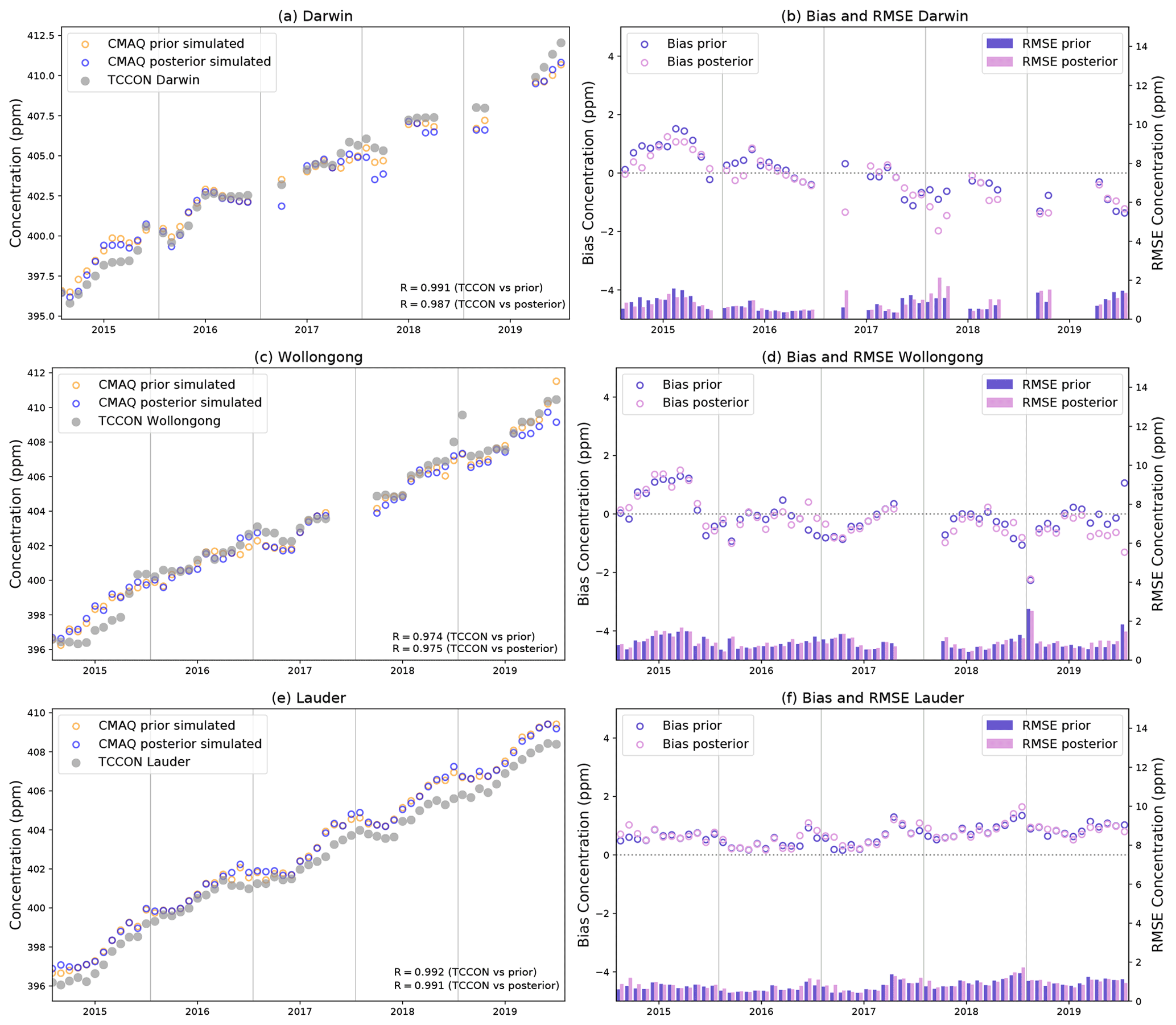
Figure 7 Comparison between the monthly mean column-averaged bias and root-mean-square error (RMSE) at the (a, b) Darwin, (c, d) Wollongong, and (e, f) Lauder TCCON sites and the CMAQ prior and posterior modelled CO₂ concentrations for 2015–2019. In panels (a), (c), and (e), the orange and blue circles represent the respective prior and posterior mean concentrations, and the grey dots represent TCCON observations.

3.4.2 Comparison with ground-based in situ measurements

Figure 8a, c, and e show the comparison between ground-based in situ measurements (Gunn point, Burncluith, Ironbark, and Cape Grim) and the prior and posterior simulated by the CMAQ model at the surface for 2015–2019, and Fig. 8b, d, and f show the bias and root-mean-square error (RMSE) from these averages. Averages were computed using data selected between 12:00 and 17:00 LT (Australian local time with respect to the individual site).

We note that the posterior column-averaged concentrations generally underestimate the observations at the Gunn Point site. The prior concentration indicates a better agreement, but biases are still significant. Some possible explanations for these results might be related to the limited vertical resolution of these retrievals and, consequently, the relative inability of OCO-2 to constrain fluxes at the scale relevant to this site (total column measurements are less sensitive at the surface than in situ sampling). Another possible explanation is that, within our model, Gunn Point is a coastal site that is affected by prevailing offshore winds. If winds come from the ocean, our fluxes are less constrained by OCO-2 retrievals (see the plot of wind directions in the Supplement, Figs. S20 and S24, for January–February).

The data for the Burncluith site span from July 2015 to May 2018 (Fig. 8b). At this site, posterior biases seem to vary seasonally. It is clear that the posterior biases are larger (relative to the prior bias) in the winter season (June, July, and August) compared with the summer season (e.g. January and February) and spring (e.g. September and October). In this period, the prior concentrations show a better agreement with the observations, with biases ranging from 0.54 to −0.46 ppm, compared with the posterior biases (range from −2.79 to −3.57 ppm). Large negative posterior biases at this site could be related to errors in the transport in the CMAQ model (e.g. associated with the parameterization scheme within the planetary boundary layer) or erroneous meteorological inputs from our WRF simulations (forcing errors). Transport errors in the vertical mixing near the surface associated with the incorrect treatment of atmospheric turbulence can cause significant biases in the simulated concentrations (Gerbig et al., 2008; Lauvaux et al., 2012). The atmospheric boundary layer mixing height is an important property in atmospheric modelling because it gives the volume of a column of air in which the fluxes contribute to the CO₂ concentration. In this study, it is difficult to quantify the likely error in the simulation of the boundary layer height because the site lacks the relevant physical measurements. A more detailed discussion of these findings is found in Sect. 4. We also did not find much improvement in the correlations at this site (Table G4).

Results for the Ironbark monitoring station are similar to Burncluith. These results were not unexpected given the stations' proximity (Fig. 2). For 2015 and 2016, validation against the Ironbark site also shows that the posterior mean concentrations were in good agreement with the observations for the summer and spring seasons. In February 2018, we see that the posterior biases were about −11.4 (RMSE of 21.61). The difference between the posterior simulation and the observations may be related to a single event visible to the surface station but not seen by OCO-2. On 7 February, Ironbark registered a CO₂ concentration of 459.87 ppm. It is possible that fires may have caused the high CO₂ concentration registered in this period (see information for February 2018 on the NASA Fire Information for Resource Management System; FIRM, 2020). From 18 to 20 April, we also see a similar event that was not captured by the inversion, causing a posterior concentration bias of −6.44 ppm (RMSE of 9.82). During these 3 d, the concentrations registered at Burncluith were greater than 450 ppm.

Cape Grim is the only site with a complete time series of observations during this period (Fig. 8d). Like Gunn Point, Cape Grim is a coastal site affected by strong westerly winds that blow from the ocean into Tasmania. In Fig. 8d, we see that there is an evident underestimation of our posterior fluxes from 2015 to 2019. However, there are some months in 2015, 2016, and 2017 for which we see a significant reduction in the prior bias. In May 2015, for example, the reduction in the biases was 87 %. For November 2016 to April 2017, the reduction in the biases was more noticeable; in April 2017, for example, we found a reduction of about 70 %. Stable winds during the period might be associated with the improvement in the biases (see Fig. S37 in the Supplement). In general, all of the negative large posterior biases for all of the months (2–5 ppm approximately) are associated with strong westerly and north-westerly winds that come from the ocean to Tasmania. As previously mentioned, Cape Grim is a coastal station whose aim is to record clean air that blows from the Southern Ocean, and it is not representative of Tasmania's air mass.

A poor fit between the posterior concentrations and surface sites raises doubts about the reliability of the OCO-2 assimilated fluxes estimated over warm temperate, tropical, and cool temperate ecosystems. Therefore, in the upcoming section, we assess the analysis of the variability in the posterior fluxes only over the savanna and sparsely ecosystems, where our posterior carbon fluxes derived by OCO-2 data are likely more trustworthy than fluxes assimilated over areas directly impacted by offshore ocean fluxes.

Figure 8 Comparison between monthly mean CO₂ concentrations (ground-based stations) at the (a) Gunn point, (c) Burncluith, (e) Ironbark, and (g) Cape Grim sites and the CMAQ prior and posterior modelled CO₂ concentrations for 2015–2019. Bias and root-mean-square error (RMSE) between the model and observations are shown in panels (b), (d), (f), and (h). The purple and violet circles in the aforementioned panels represent the respective prior and posterior concentration biases, and the purple and violet bars represent the respective prior and posterior RMSE values.

3.5 Australia's carbon flux anomalies

Figure 9a and b illustrate the 3-month running mean of the prior and posterior flux anomalies and the 3-month running means of EVI, rainfall, and air temperature anomalies for the 2015–2019 period aggregated over sparsely vegetated and savanna ecosystems. Figure 10 shows the spatial distribution pattern of the annual anomalies of the posterior flux estimate for the 2015–2019 period.

It is clear that the anomalous prior and posterior carbon land sink recorded over the sparsely vegetated ecosystem from August 2016 to April 2017 is likely due to the combination of a higher-than-average increase in land productivity (positive EVI anomalies) and rainfall (positive rainfall anomalies) as well as a lower-than-average decrease in air temperature (negative temperature anomalies). It is also evident that the strong carbon release (positive carbon flux anomalies) recorded after April 2017 is due to a lower-than-average greenness of the vegetation (negative EVI anomalies) and rainfall (negative rainfall anomalies) as well as an increase in the air temperature (positive temperature anomalies). In this ecoregion, we found that the temporal correlation between EVI anomalies and carbon flux anomalies is in better agreement with the posterior ($R=-\mathrm{0.5}$) than the prior ($R=-\mathrm{0.32}$) anomalies. The posterior and EVI correlations become even stronger when we see them at each grid point Fig. 11b (R=0.5–0.9). Spatial averaging smooths grid point anomalies and, thus, dilutes signals. The spatial distribution of correlations between rainfall anomalies (Fig. 11d), temperature anomalies (Fig. 11f), and posterior carbon anomalies also improved in some areas in this large ecosystem.

Similar to the findings for sparsely vegetated regions, we also see a higher-than-average increase in land productivity (positive EVI anomalies) and rainfall as well as a decrease in air temperature recorded from August 2016 to April 2017 over the savanna ecosystem. However, unlike the results for sparsely vegetated regions, the carbon sink anomaly only coincides with the negative posterior carbon anomaly in 2016. In 2017, we see that the positive EVI and rainfall as well as the negative anomalies recorded from January to April do not align with the larger-than-average posterior carbon release in this period. We believe that the few OCO-2 soundings found in this period limit the potential of our inversion to constrain the surface fluxes in the savanna ecosystem (see Fig. S2a, b, and c in the Supplement). We found similar results in September and November 2017. As mentioned in Sect. 3.1, there was a long data outage of 51 d from August to September 2017. In September, the number of OCO-2 observations in Australia was only 221, and most of the soundings were seen over sparsely vegetated regions (in central Australia) compared with the savanna ecosystem (see Fig. S2h and i in the Supplement). In 2019, we also see that a lower-than-average land productivity, in combination with a rainfall deficit and an increase in temperature, led to a stronger carbon release into the atmosphere. In this category, the temporal correlation between the posterior anomalies and EVI anomalies was moderate ($R=-\mathrm{0.38}$) compared with the prior flux anomalies and EVI anomalies ($R=-\mathrm{0.52}$). We note that the time series temporal correlation between EVI anomalies and posterior anomalies at the grid-cell-scale resolution (Fig. 11a) is slightly stronger for the prior than the posterior correlations (Fig. 11b). Similar results were found between the link of the rainfall and posterior flux anomalies, where the correlation tends to degrade compared with the prior. The spatial correlation between temperature anomalies and posterior correlation is more variable, and we see that correlations for the posterior flux anomalies are stronger in the north-west area of the continent.

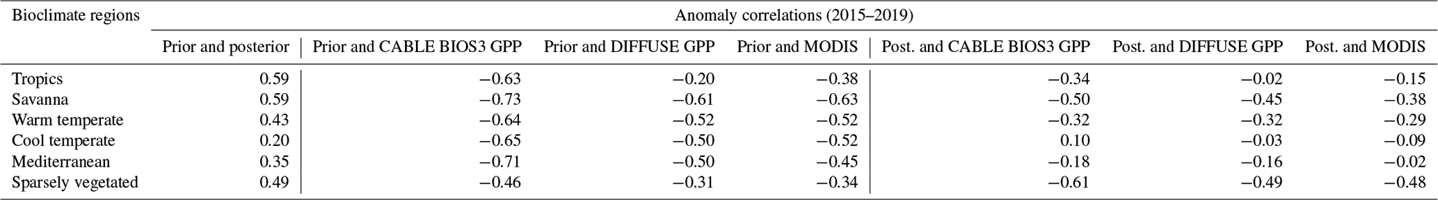
In general, the better agreement between posterior, climate, and vegetation parameters over regions with sparse vegetation is because the CABLE model likely underestimates GPP anomalies. We found that the correlation between the posterior anomalies and CABLE BIOS3, DIFFUSE, and MODIS GPP anomalies was stronger than that for the prior anomalies. For example, the correlation between the prior and CABLE BIOS3 GPP anomalies was −0.46 compared with the posterior ($R=-\mathrm{0.61}$). Correlations between the posterior anomalies and DIFFUSE and MODIS GPP (−0.5) were also stronger than the prior ($R=-\mathrm{0.3}$) (more details in Table D2). These findings are significant for Australia because they suggest that our OCO-2 inversion might likely be better at capturing the anomalies of this ecosystem (the largest ecosystem in Australia) compared with the biosphere–land model.

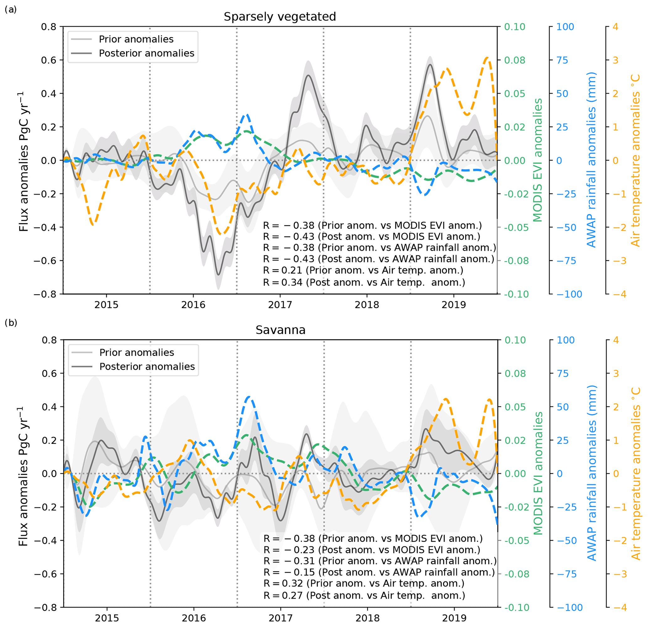
Figure 9 Time series of the 3-month running mean posterior (black line) and prior (grey line) terrestrial carbon flux anomalies (PgC yr⁻¹) and 3-month running mean EVI anomalies (turquoise dashed line) between 2015 and 2019 aggregated by two agroclimatic regions: (a) sparsely vegetated and (b) savanna ecosystems. Anomalies over tropical, warm temperate, cool temperate, and Mediterranean ecosystems are shown in Appendix D (Fig. D1). The grey shaded area represents a 1.0 standard deviation range around the mean for the prior and posterior flux uncertainty.

Figure 10 Spatial distribution maps of the annual posterior terrestrial carbon flux anomalies (gC m⁻² yr⁻¹) for 2015–2019 (a, b, c, d, e). Negative anomalies correspond to a larger-than-average uptake of carbon by land ecosystem, whereas positive anomalies correspond to a larger-than-average release of carbon to the atmosphere from the land.

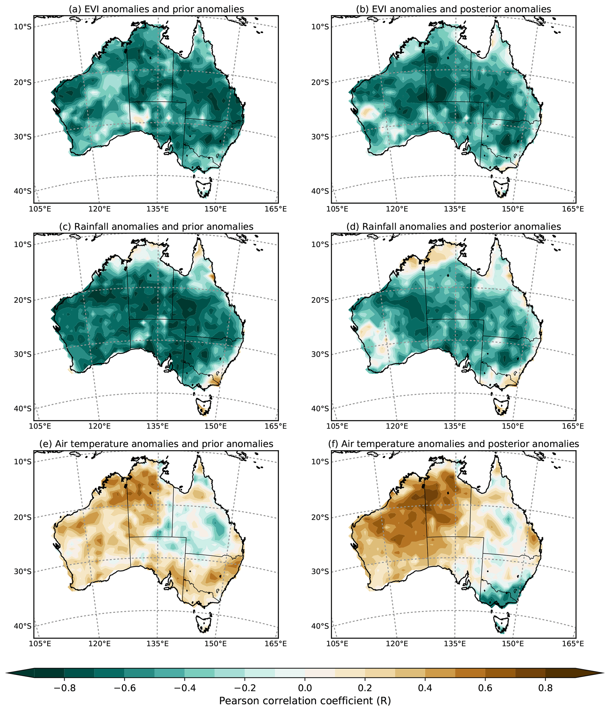
Figure 11 Spatial map of the monthly temporal correlation between (a, b) EVI prior and posterior anomalies, (c, d) rainfall prior and posterior anomalies, and (e, c) air temperature prior and posterior anomalies for the 2015–2019 period.

4 Discussion

In Sect. 3.4, we saw that validating the posterior concentrations against the current Australian greenhouse gas monitoring system is challenging due to the small number of stations across the continent (approximately five). In addition, some of these sites, such as Cape Grim, provide no meaningful constraint on Australian fluxes and, therefore, leave the question of accuracy in the posterior carbon fluxes unanswered over savanna and sparsely vegetated regions, where our inversion suggests a stronger carbon sink for the study period compared with the prior estimate made by the biosphere model.

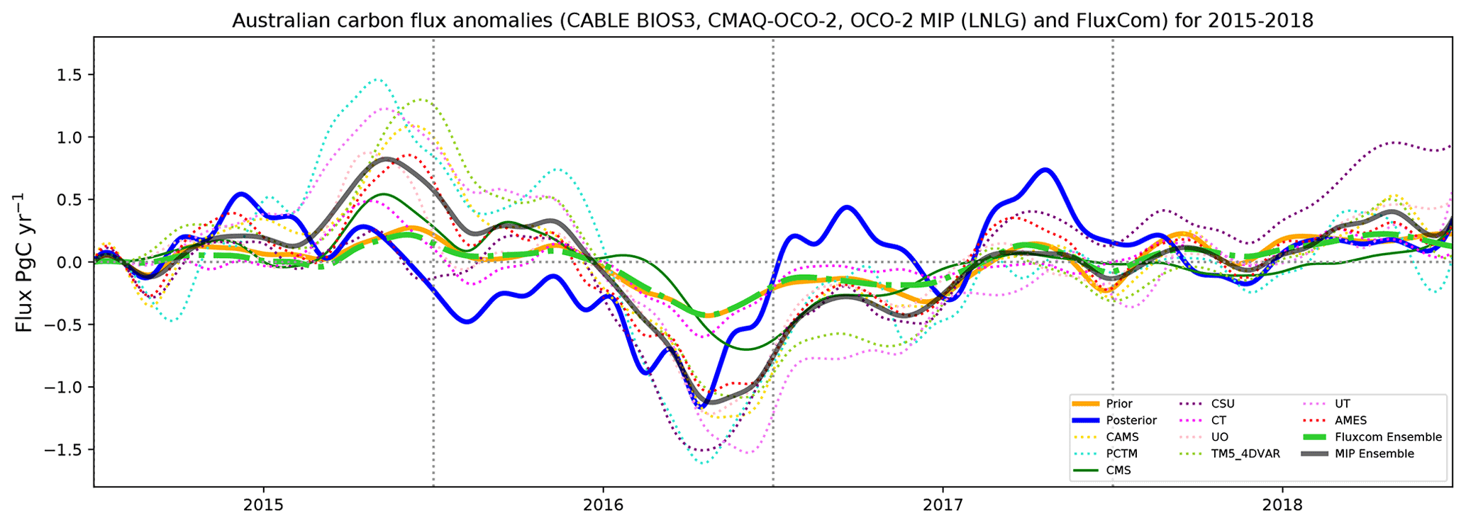
Figure 12 Comparison between monthly mean posterior (blue line), prior (orange line), FLUXCOM ensemble mean (green line), OCO-2 MIP ensemble (black line) carbon fluxes, and the monthly carbon fluxes from the nine models that participate in OCO-2 MIP: AMES, PCTM, CAMS, CMS-Flux, CSU, CT, OU, TM5-4DVAR, and UT (in PgC yr⁻¹).

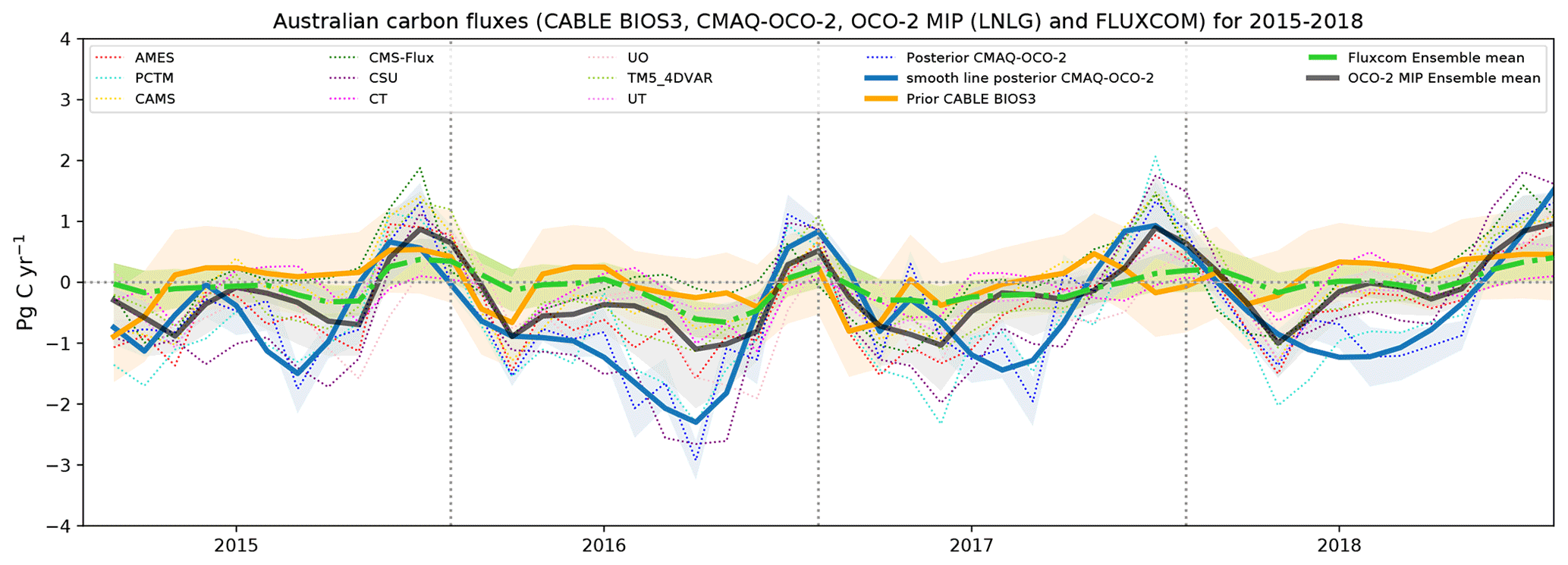
Figure 13 Comparison between 3-month running mean posterior (black line), prior (grey orange), FLUXCOM ensemble, OCO-2 MIP ensemble carbon flux anomalies, and 3-month running mean anomalies of the nine models that participate in OCO-2 MIP: AMES, PCTM, CAMS, CMS-Flux, CSU, CT, OU, TM5-4DVAR, and UT (in PgC yr⁻¹).

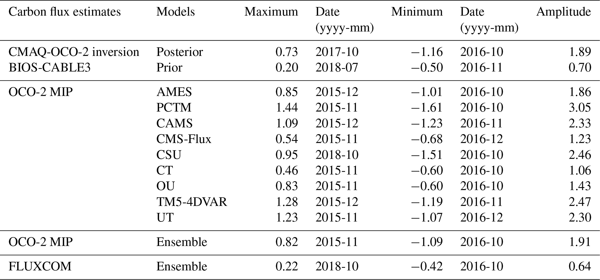
Table 3 Summary of the peak-to-peak amplitude of 3-month running mean posterior, prior, and FLUXCOM flux anomalies as well as 3-month running mean anomalies of the nine different models from OCO-2 MIP (in PgC yr⁻¹).

To assess and discuss how well our monthly assimilated OCO-2 carbon fluxes align the current understanding of the Australian carbon cycle, we compare our results to other global products: OCO-2 MIP global inversions (AMES, PCTM, CAMS, CMS-Flux, CSU, CT, OU, TM5-4DVAR, and UT) and FLUXCOM for 2015–2018 (Fig. 12). The annual OCO-2 MIP ensemble mean of carbon fluxes shown in Fig. 12 suggests that Australia was a carbon sink of −0.26 ± 0.22 for 2015–2018, similar to our posterior flux estimate (−0.52 ± 0.08 PgC yr⁻¹) considering the OCO-2 MIP ensemble spread of the nine models as representing the uncertainty. The annual FLUXCOM ensemble mean also suggests that Australia was a slight carbon sink of −0.06 ± 0.04. In terms of seasonality, we can observe (from Fig. 12) that, for several periods between 2015 and 2018, the monthly mean of our posterior carbon fluxes falls within the uncertainties of the OCO-2 MIP ensemble mean, except for some months in winter. For example, we notice that the large carbon sink estimated by our inversion (−2.92 ± 0.27 PgC yr⁻¹) in August 2016 does not fall within the ensemble monthly MIP mean of that period (−1.28 ± 0.78 PgC yr⁻¹). However, the carbon flux estimate derived by the PCTM (−2.31 PgC yr⁻¹) and CSU (−2.66 PgC yr⁻¹) global models shows similar results to our flux estimate. These findings are also observed throughout 2015, 2017, and 2018, when our posterior carbon flux estimates closely follow PCTM and CSU seasonal patterns. The seasonality of FLUXCOM agrees with our assimilated fluxes, mostly in summer but not in winter.

We also studied the carbon flux anomalies derived by OCO-2 MIP and FLUXCOM and compared them with the prior and posterior flux anomalies (3-month running mean) that we have discussed throughout this study (Fig. 13). In Fig. 13, we see that all carbon flux estimates agree that 2016 was the period in which Australia recorded the largest carbon uptake relative to the 2015–2018 mean. Throughout this study, we saw that 2016 was a year in which Australia recorded above-average precipitation and low temperatures that certainly drove the increase in vegetation productivity across the country. Similar findings were reported by Haverd et al. (2016) for 2011; their study suggested that the variations in carbon fluxes over Australia's semi-arid ecosystems show a direct physiological response of vegetation productivity to water availability fluctuations. Other regional studies conducted in Africa (e.g. Williams et al., 2008; Archibald et al., 2009; Merbold et al., 2009) have also indicated that the interannual carbon fluctuations in semi-arid ecosystems largely depend on water availability, which is driven by variations in rainfall between years. Water availability is the most important factor that controls the vegetation productivity of ecosystems across most of Australia, such as grasslands and shrublands/desert (see Fig. 2 in Churkina and Running, 1998).

In terms of the amplitude of carbon flux anomalies, we can see that the prior and the FLUXCOM anomalies exhibit a lower amplitude than the one derived by our inversion and the majority of the models in the MIP. Australian FLUXCOM estimates are likely not a good representation of the carbon flux estimates for the continent, given the sparsity of the flux tower network. FLUXCOM carbon fluxes use machine learning methods to empirically upscale flux tower data. In Australia, the number of OzFlux monitoring sites is small (approximately 30 towers), and most of the flux towers are located far away from semi-arid/arid ecosystems. This is relevant for Australia because semi-arid/arid ecosystems represent about 70 % of the Australian landscape.

With respect to OCO-2 MIP global inversions, we observe that five global inversions (PCTM, CMS-Flux, CT, OU, and UT) agreed with our findings for 2016 and suggested October as the month of peak uptake. The ensemble mean of FLUXCOM also agrees with our results (−0.42 PgC yr⁻¹); however, the size of the uptake is half of our estimates (−1.12 PgC yr⁻¹). In terms of the peak of carbon release, there is no agreement between MIP, FLUXCOM, and prior and posterior carbon estimates. We observe that almost all OCO-2 MIP inversions agree that the largest outgassing occurred in November 2015. Our inversion places the maximum outgassing in October 2017, whereas the FLUXCOM and the prior have the maximum outgassing period in October and July 2018 respectively.

The analysis of the interannual (peak-to-peak) variability shows that PCTM (3.05 PgC yr⁻¹) and CSU (2.46 PgC yr⁻¹) produce the largest amplitude of variability compared with our prior (0.70 PgC yr⁻¹) and posterior (1.89 PgC yr⁻¹) anomalies. We also note that OU and AMES exhibit the lowest carbon amplitude of the variability, with values of 1.06 and 1.86 respectively. The disagreement between the global inversion and our study might also be driven by transport differences (Basu et al., 2018; Schuh et al., 2019).

The larger seasonal cycle amplitude of the anomalies suggested by our regional inversion and OCO-2 MIP compared with the flux anomalies derived by the CABLE model and FLUXCOM raises some questions. For example, why do Australia's semi-arid ecosystems capture more carbon dioxide (based on our OCO-2 inversion) than the process-based model estimate? Could it be possible that the larger posterior carbon uptake and its larger anomalies estimated by the inversion (relative to the prior and FLUXCOM) are because the CABLE model is not well calibrated against the insufficient number of eddy covariance flux towers across the continent? Could the remaining OCO-2 biases in version 9 and potential errors in the transport model be causing deviation from the true flux? More work needs to be done to reconcile and disentangle what is being found by the inversions and the Australia CABLE model. In future work, we could run this regional inversion using the latest version of OCO-2 data (version 10) in combination with ocean glint data, for which recent verifications confirm reductions in both the bias and standard deviation compared with the TCCON data (OCO-2 Data Quality Statement, 2020). Another direction for future work would be to explore the impact of transport model errors on the resulting assimilated OCO-2 fluxes. Such assessment could be done by choosing, for example, different planetary boundary schemes within the CMAQ model. As mentioned in Sect. 3.4.2, a misrepresentation of vertical mixing near the surface in atmospheric transport models leads to uncertainties in modelled CO₂ mixing ratios. Mixing within the planetary boundary layer influences the redistribution of the surface fluxes to the atmospheric column. Another way of evaluating the transport error of the model would be through a model intercomparison. This approach is well known in the global inversion TransCom group community (Law et al., 2008; Peylin et al., 2013; Basu et al., 2018); examples of such intercomparisons are the recent Model Intercomparison Project (MIP), organized by the OCO-2 Science Team (Crowell et al., 2019; Peiro et al., 2022), and the recent European atmospheric transport inversion comparison (EUROCOM) project (Monteil et al., 2020).

Finally, we could say that previous inversion studies over Australia have been limited by the lack of in situ data. The OCO-2 data certainly allow for a quantum leap in resolution, but this is still reasonably coarse, especially when one recalls that the prior covariance structures we use impose smooth variations up to the correlation length of 500 km. Instruments with scanning geometries that allow higher-resolution observations, such as OCO-3 (Eldering et al., 2019), may significantly improve the available resolution of fluxes. This is particularly important when assessing the roles of drivers, such as rainfall, that may vary on smaller scales. We also note that continuing improvement of the OCO retrievals themselves should allow the joint assimilation of land and ocean measurements, hopefully improving the visibility of coastal fluxes and the comparison with coastal in situ measurements such as Cape Grim and Gunn Point, as shown by Villalobos et al. (2021).

5 Conclusions

We estimated monthly carbon fluxes over Australia for 2015–2019, based on the assimilation of Orbiting Carbon Observatory-2 (OCO-2) satellite data (land nadir and glint data, version 9). We investigated the effect of vegetation productivity (using EVI anomalies as a proxy) and climate driver variations such as rainfall and air temperature on the Australian terrestrial carbon flux variability. The mean of our 5-year inversion suggests that Australia was a −0.46 ± 0.08 PgC yr⁻¹ carbon sink, which was driven partly by large carbon uptake (−1.04 PgC yr⁻¹) recorded in 2016 over savanna and sparsely vegetated ecosystems. We found that negative carbon flux anomalies recorded in this period over these ecosystems coincide with an increase in the vegetation greenness (positive EVI anomalies) driven by higher-than-average rainfall anomalies and lower-than-average air temperature anomalies. The 2017 sink over Australia also contributed to the 2015–2019 long-term mean, but its contribution was not as significant as that for 2015 and 2016. Negative carbon flux anomalies recorded in 2017 also coincided with positive rainfall anomalies and below-average temperatures in that period over areas with sparse vegetation. In 2018, we did not find significant terrestrial flux anomalies across Australia, and 2019 was mainly affected by positive carbon flux anomalies, which were also in line with a rainfall deficit and positive temperature anomalies.

With respect to the validation of our inversion with independent data, we found it challenging to validate our posterior column-averaged concentration using the current Australian monitoring sites. Despite the fact that the posterior concentration biases at the TCCON monitoring site were less than 1.0 ppm for several periods between 2015 and 2019, OCO-2 data were not able to reduce prior biases significantly. We associate this slight improvement or lack of improvement with the fact that these monitoring stations are strongly affected by ocean fluxes, for which no OCO-2 data were considered. Similar findings were reported for in situ measurements at coastal sites such as Cape Grim and Gunn Point. Despite the weak comparison with independent monitoring data, the comparisons to the OCO-2 MIP global inversion for 2015–2018 and the FLUXCOM ensemble mean present similar results to our regional inversion, suggesting that the year 2016 was a period in which Australia acted as a strong carbon (CO₂) sink.

Appendix A: Histograms: the CMAQ model and OCO-2 differences

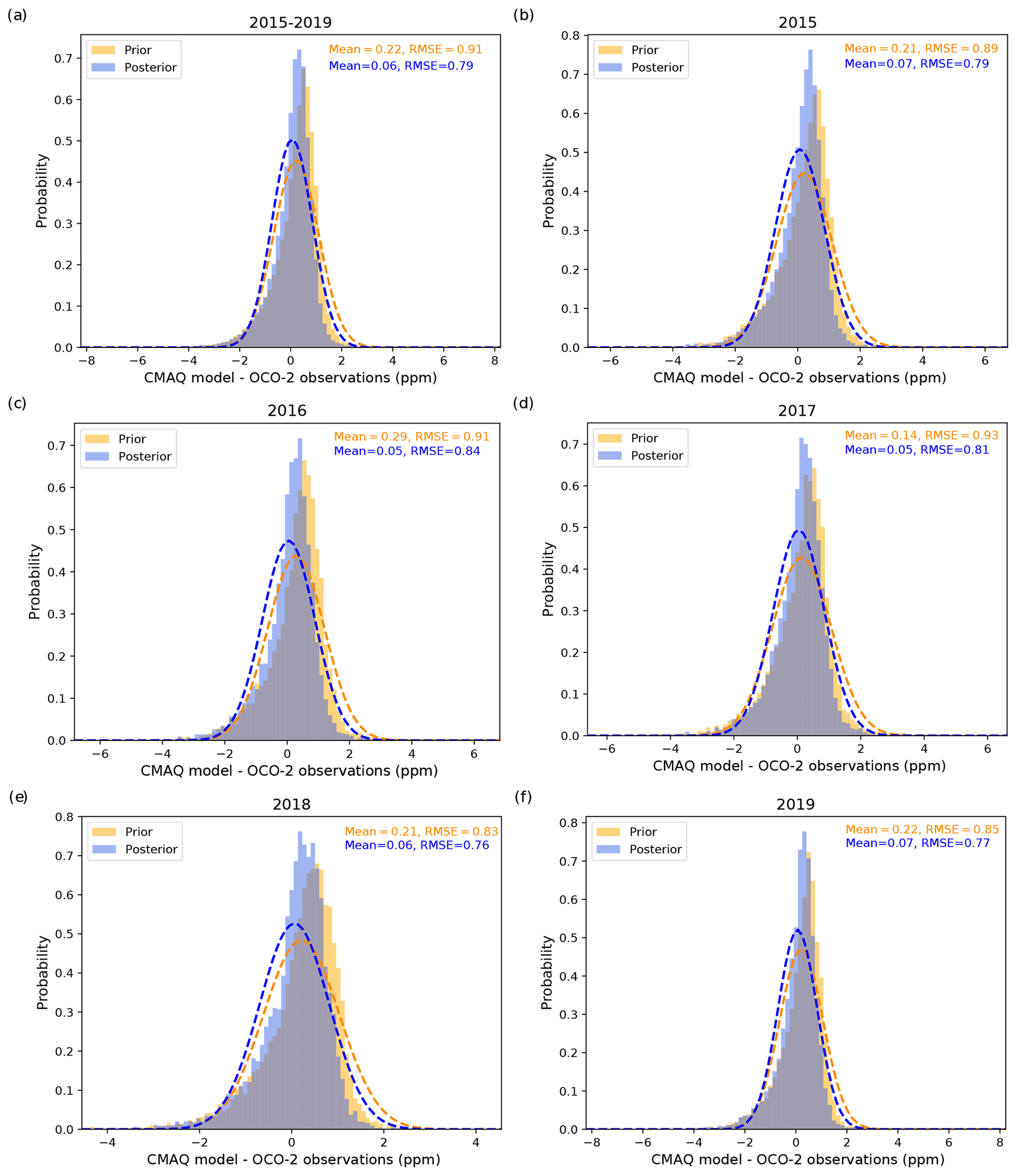
Figure A1 Probability density distribution of the difference between the CMAQ column-averaged CO₂ concentration and OCO-2 observations (in ppm). The orange histogram presents the prior CMAQ column-averaged simulated concentration minus OCO-2, whereas the blue histogram presents the posterior column-averaged simulated concentration minus the OCO-2. The mean differences and the RMSE are indicated in the legend.

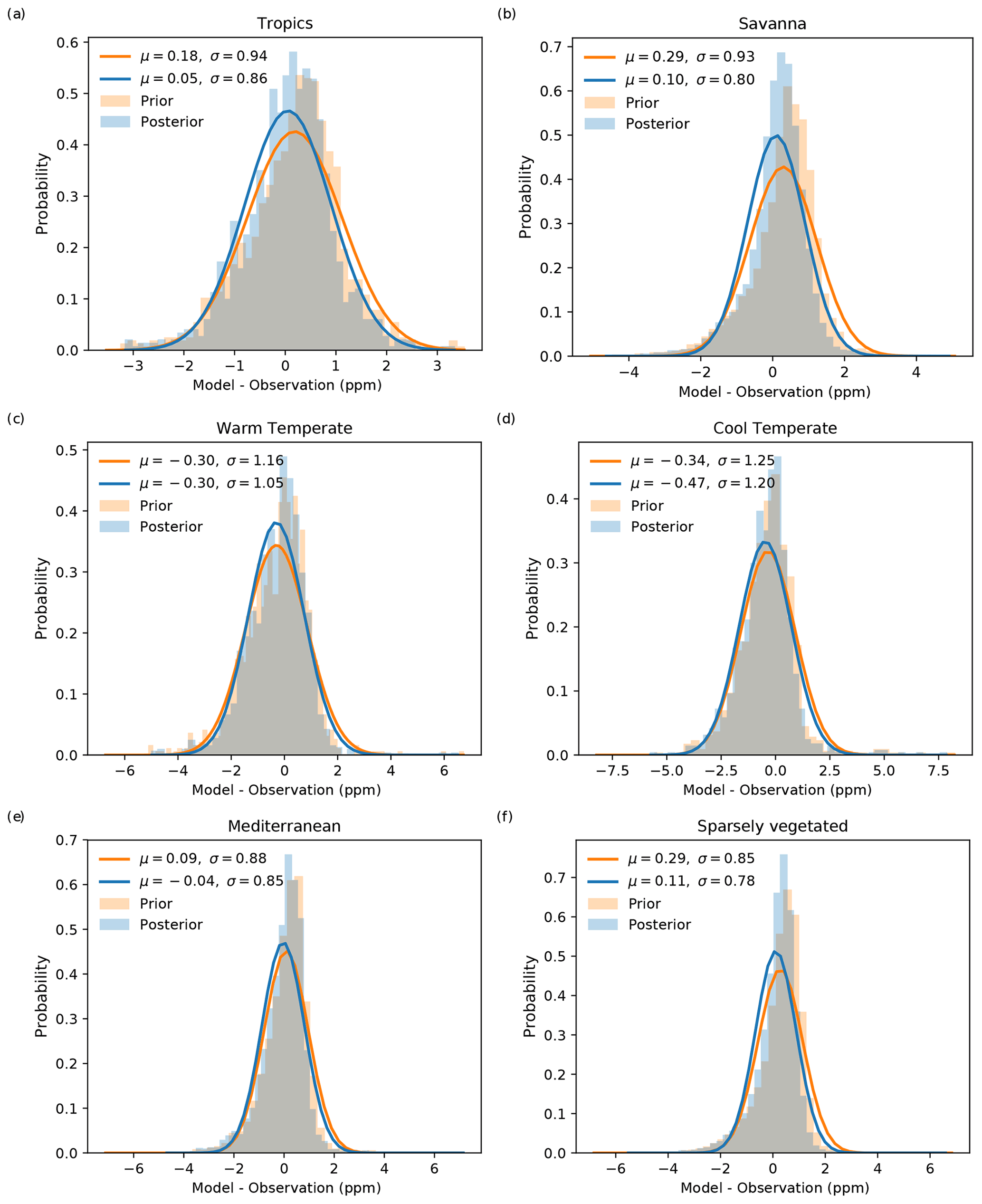
Figure A2 Probability density distribution of the difference between the CMAQ column-averaged CO₂ concentration and OCO-2 observations aggregated by six bioclimatic classifications (in ppm). The orange histogram presents the prior CMAQ column-averaged simulated concentration minus OCO-2, whereas the blue histogram presents the posterior column-averaged simulated concentration minus the OCO-2. The mean differences and the RMSE are indicated in the legend.

Appendix B: Spatial distribution of the prior and posterior annual means (2015–2019)

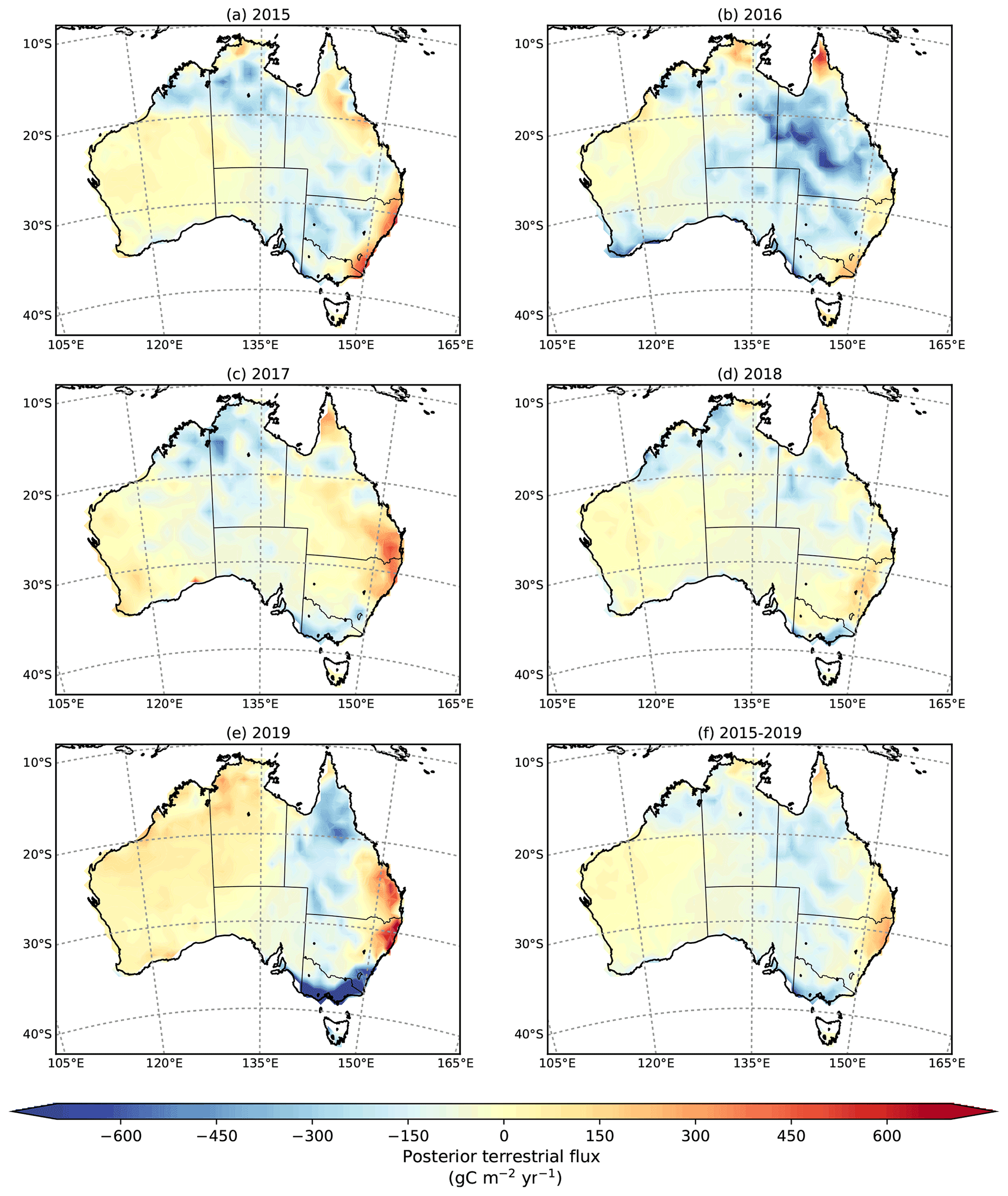
Figure B1 Posterior fluxes assimilated using LNLG OCO-2 satellite observations averaged for 2015–2019 (fossil fuel emissions are excluded).

Figure B2 Prior fluxes derived by the CABLE model using the BIOS3 set-up in combination with fire emissions selected by GFED averaged for 2015–2019 (fossil fuel emissions are excluded).

Appendix C: Climatological seasonal cycle and GPP anomalies (2015–2019)

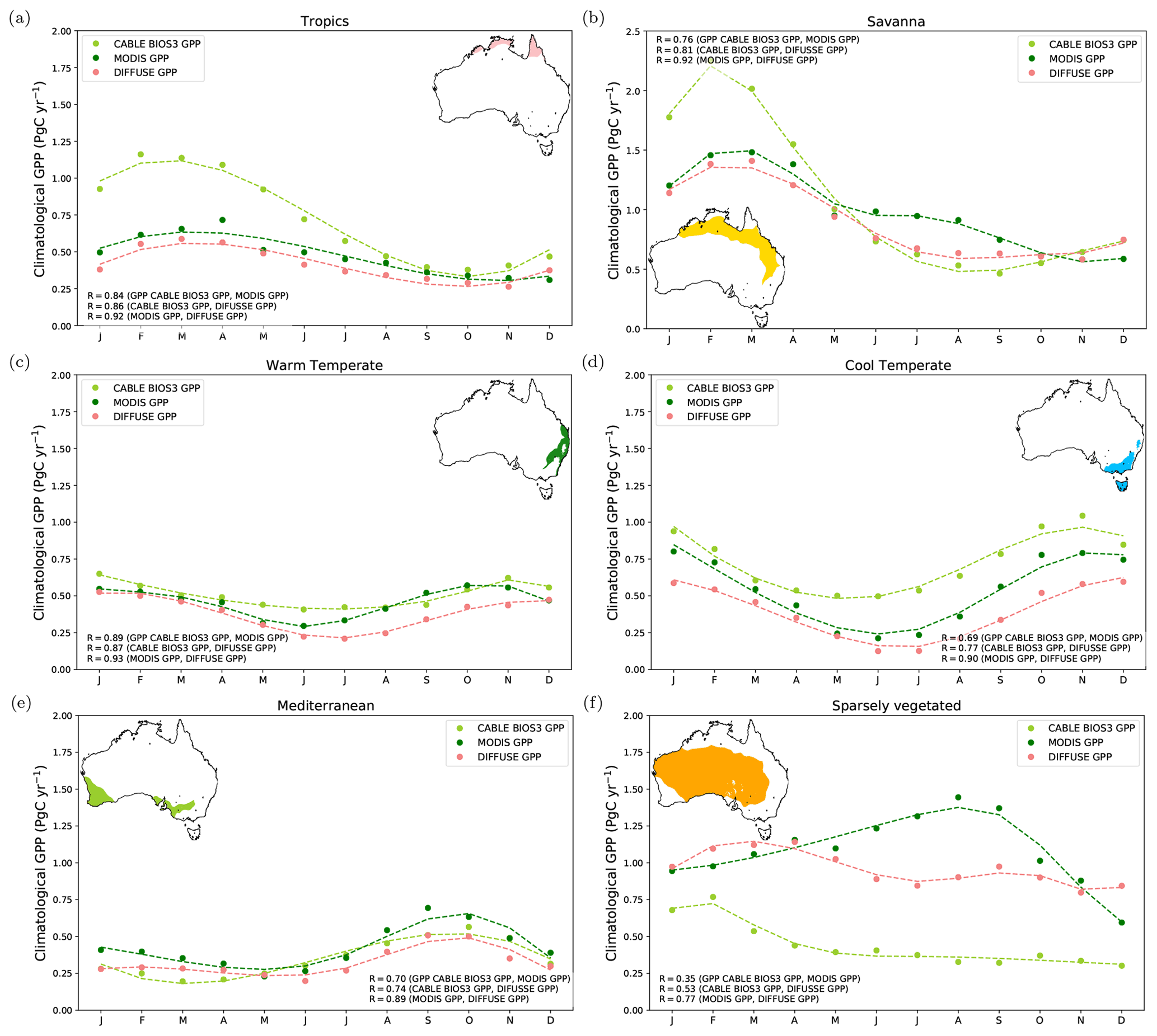
Figure C1 Climatological seasonal cycle of the GPP (2015–2019) derived from the CABLE BIOS3 model (light green dashed line), MODIS (dark green dashed line), and the DIFFUSE model (pink dashed line).

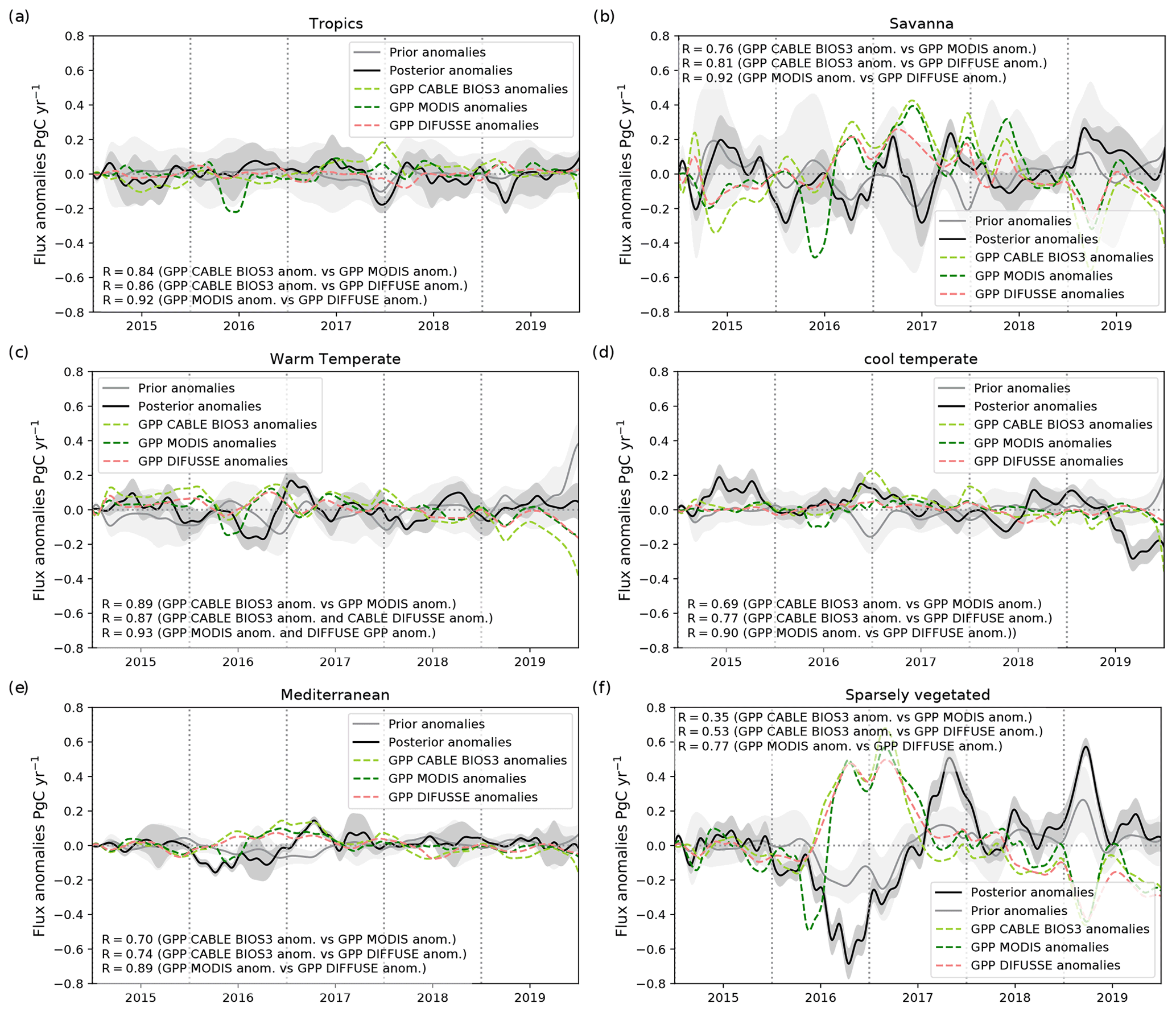
Figure C2 Time series of the 3-month running mean GPP anomalies derived from the CABLE BIOS3 model (light green dashed line), MODIS (dark green dashed line), and the DIFFUSE model (orange dashed line) between 2015 and 2019.

Appendix D: Carbon flux anomalies aggregated by bioclimatic regions

Figure D1 Time series of the 3-month running mean posterior (black line) and prior (grey line) terrestrial CO₂ flux anomalies (PgC yr⁻¹) and 3-month running mean EVI anomalies (turquoise dashed line) between 2015 and 2019 aggregated by four agroclimatic regions: (a) tropics, (b) warm temperate, (c) cool temperate, and (d) Mediterranean. The grey shaded area represents a 1.0 standard deviation range around the mean for the prior and posterior flux uncertainty.

Appendix E: Spatial distribution of OCO-2 soundings (land nadir and glint data) over the CMAQ domain for 2015

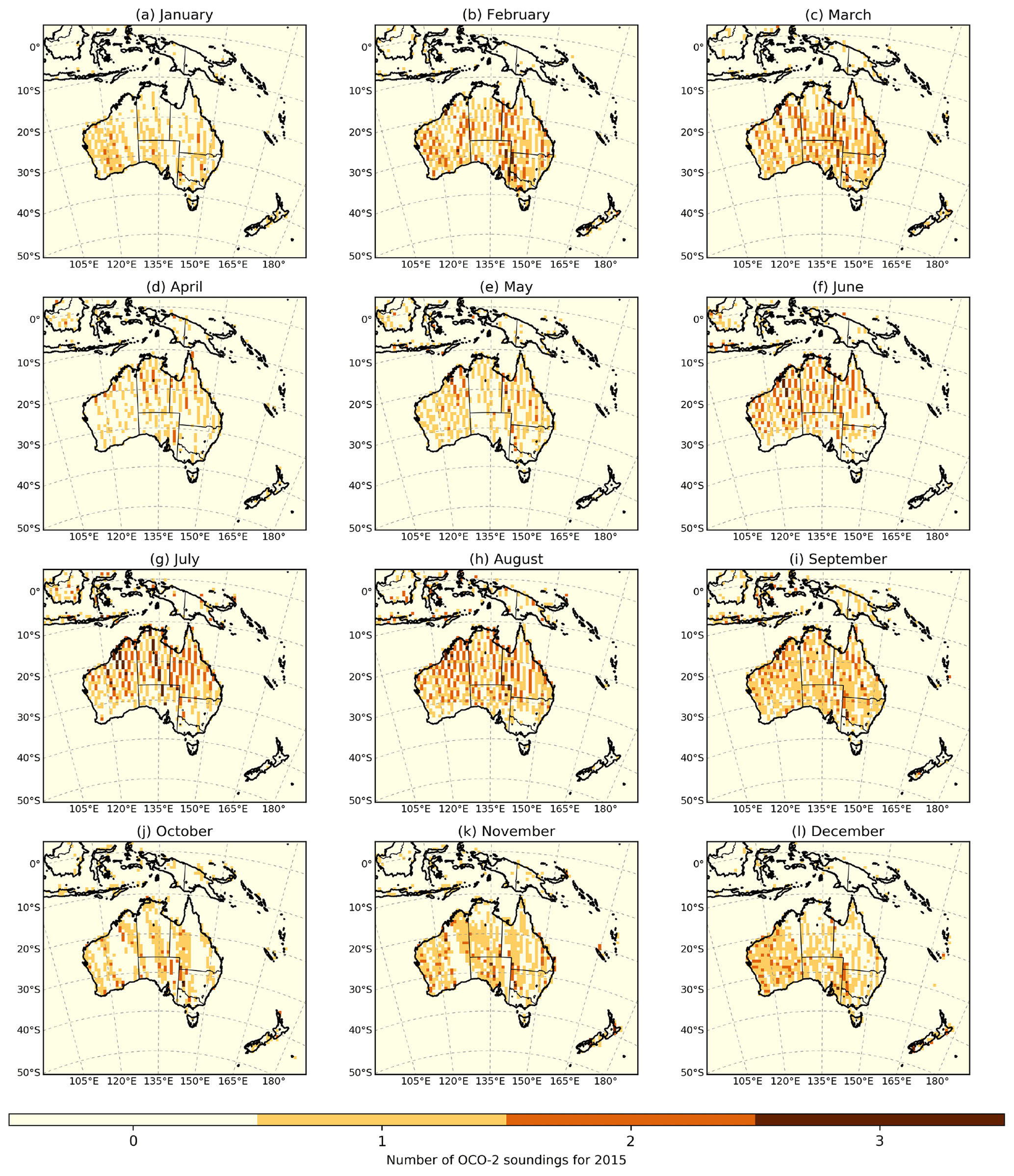
Figure E1 Spatial distribution of OCO-2 soundings (land nadir and glint data) over the CMAQ domain for 2015.

Appendix F: Analysis of the residual TCCON

Table F1 Analysis of the residual between CMAQ prior and posterior simulation values and the TCCON Darwin site for the 2015–2019 period, showing the averaged bias (Bias), root-mean-square error (RMSE), and Pearson coefficient (R).

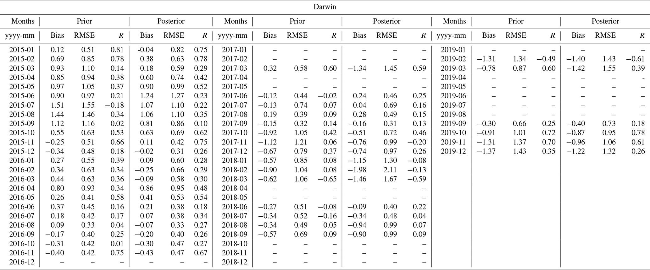
Table F2 Analysis of the residual between CMAQ prior and posterior simulation values and the TCCON Lauder site for the 2015–2019 period, showing the averaged bias (Bias), root-mean-square error (RMSE), and Pearson coefficient (R).

Table F3 Analysis of the residual between CMAQ prior and posterior simulation values and the TCCON Wollongong site for the 2015–2019 period, showing the averaged bias (Bias), root-mean-square error (RMSE), and Pearson coefficient (R).

Appendix G: Analysis of the residual in situ data

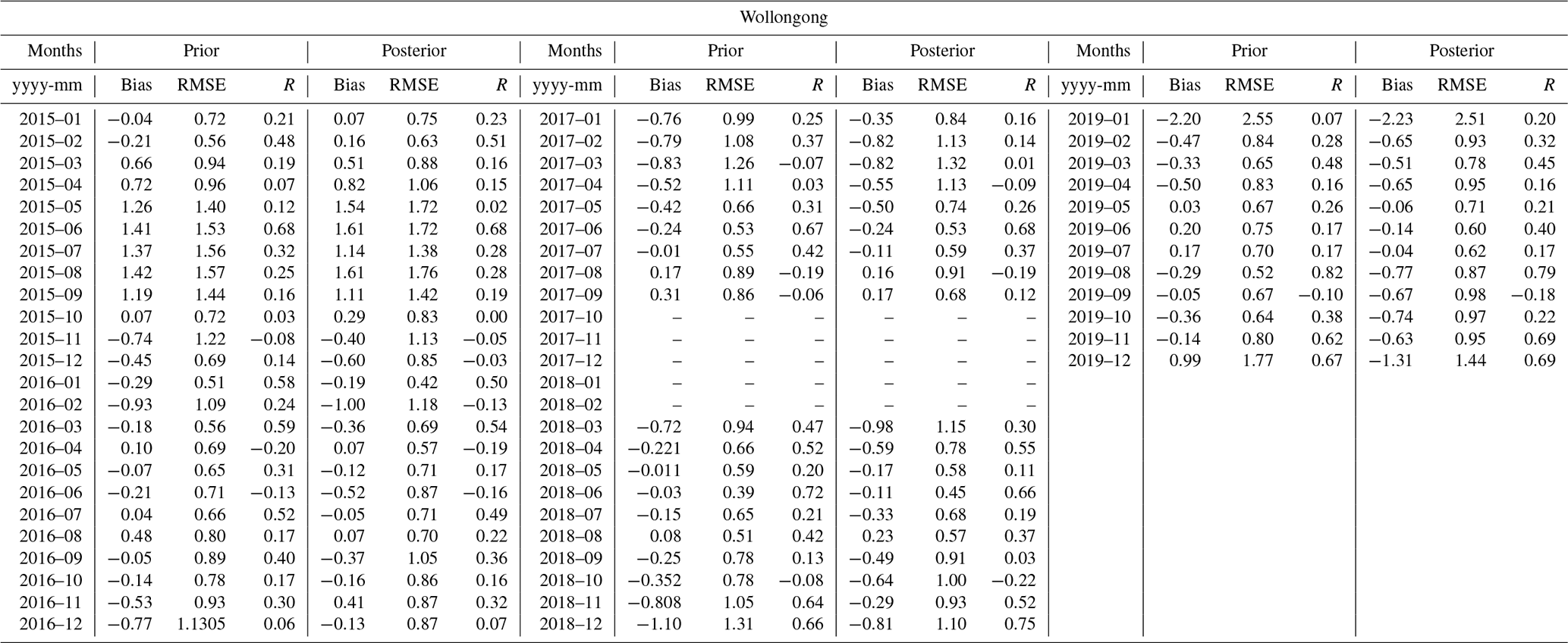
Table G1 Analysis of the residual between CMAQ prior and posterior simulation values and the Cape Grim site for the 2015–2019 period, showing the averaged bias (Bias), root-mean-square error (RMSE), and Pearson coefficient (R).

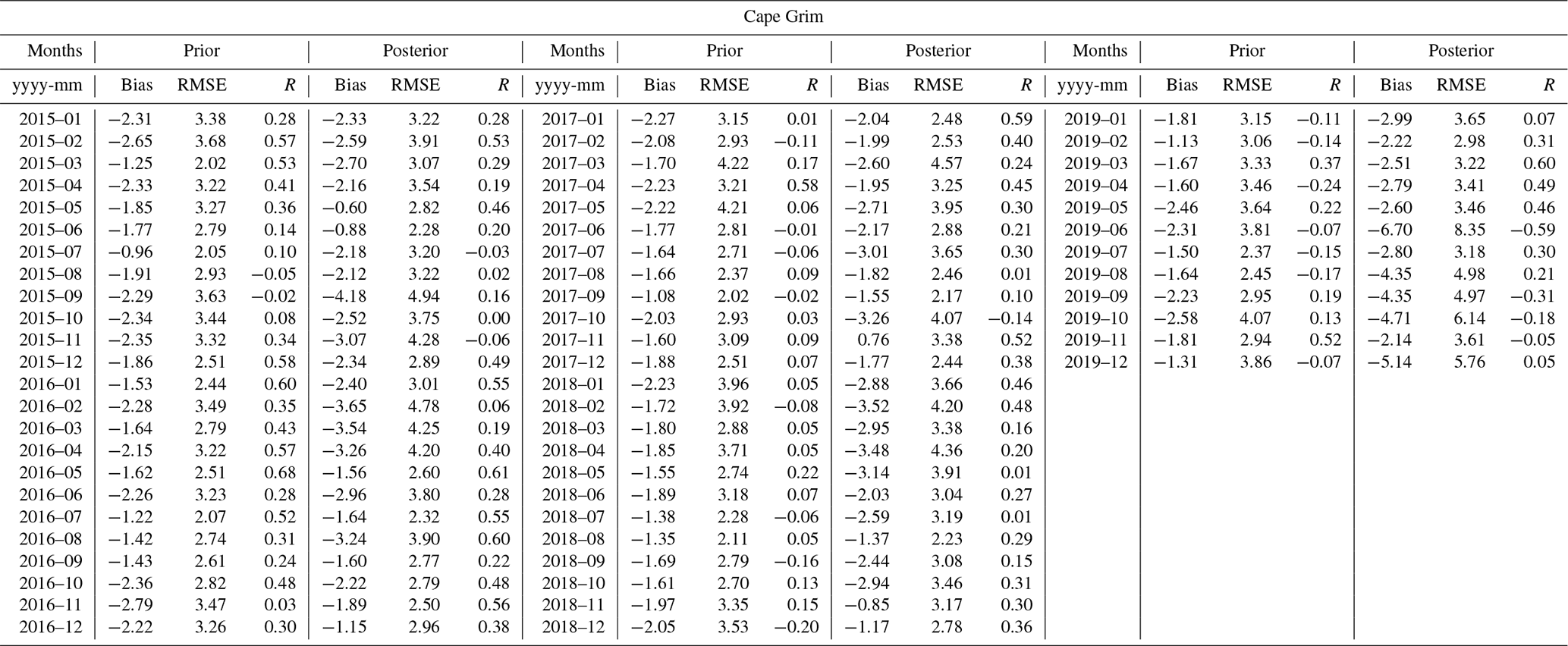
Table G2 Analysis of the residual between CMAQ prior and posterior simulation values and the Gunn Point site for the 2015–2019 period, showing the averaged bias (Bias), root-mean-square error (RMSE), and Pearson coefficient (R).

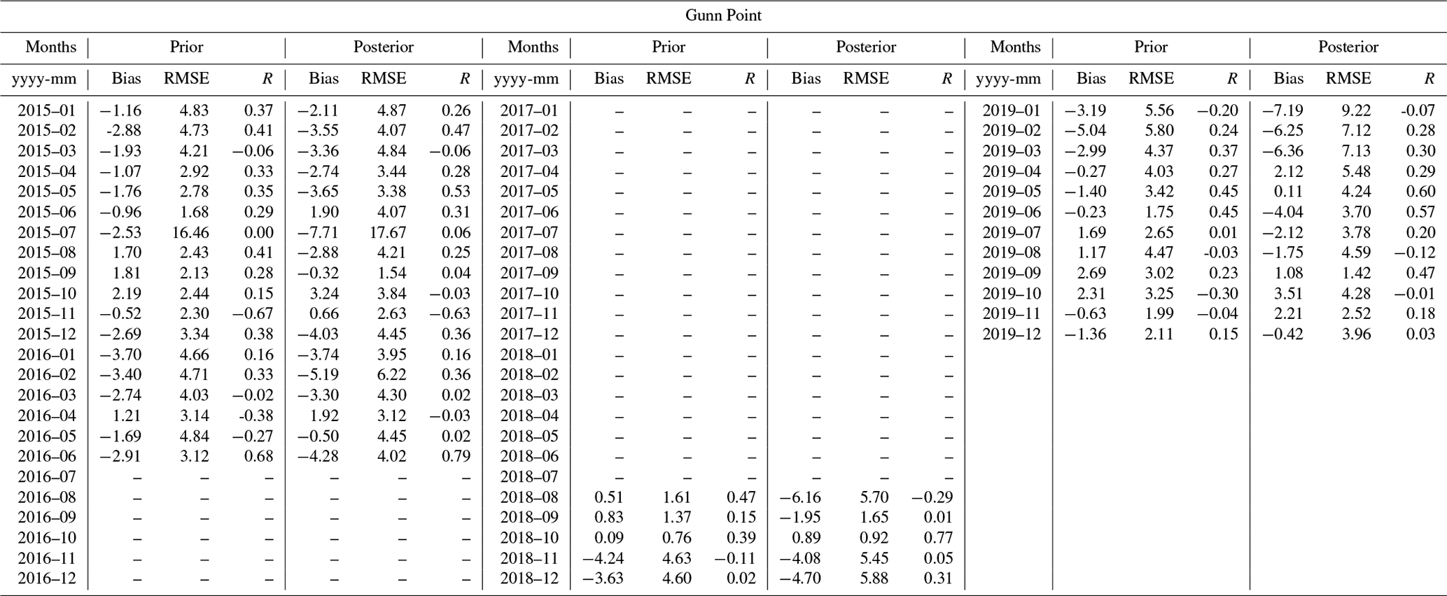
Table G3 Analysis of the residual between CMAQ prior and posterior simulation values and the Iron bark site for the 2015–2019 period, showing the averaged bias (Bias), root-mean-square error (RMSE), and Pearson coefficient (R).

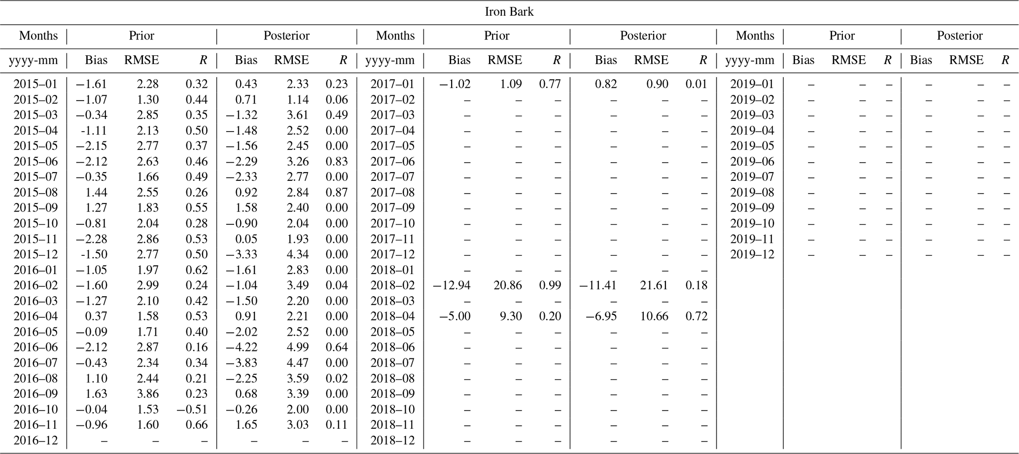
Table G4 Analysis of the residual between CMAQ prior and posterior simulation values and the Burncluith site for the 2015–2019 period, showing the averaged bias (Bias), root-mean-square error (RMSE), and Pearson coefficient (R).

Appendix H: Prior, posterior, and GPP flux anomaly correlation analysis

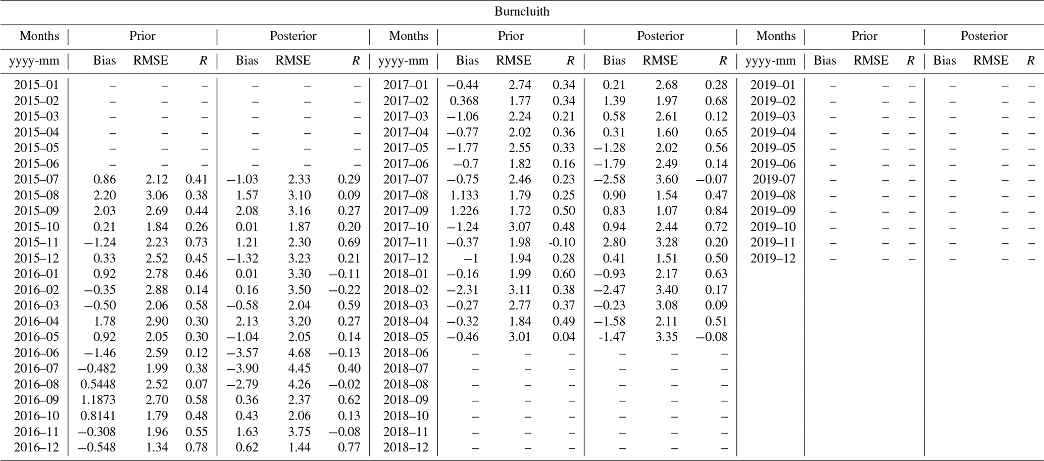
Table H1 The Pearson correlation (R) values of prior and posterior climatological seasonal fluxes with GPP fluxes derived from the respective CABLE BIOS3, MODIS, and DIFFUSE models.

Table H2 The Pearson correlation (R) values of prior and posterior flux anomalies with GPP anomalies derived from the respective CABLE BIOS3, MODIS, and DIFFUSE models.