the Creative Commons Attribution 4.0 License.
the Creative Commons Attribution 4.0 License.
 | 22 Feb 2022
The contribution of coral-reef-derived dimethyl sulfide to aerosol burden over the Great Barrier Reef: a modelling study
Matthew T. Woodhouse
Steve Utembe
Robyn Schofield
Simon P. Alexander
Joel Alroe
Scott D. Chambers
Zhenyi Chen
Luke Cravigan
Erin Dunne
Ruhi S. Humphries
Graham Johnson
Melita D. Keywood
Todd P. Lane
Branka Miljevic
Yuko Omori
Alain Protat
Zoran Ristovski
Paul Selleck
Hilton B. Swan
Hiroshi Tanimoto
Jason P. Ward
Alastair G. Williams
Coral reefs have been found to produce the sulfur compound dimethyl sulfide (DMS), a climatically relevant aerosol precursor predominantly associated with phytoplankton. Until recently, the role of coral-reef-derived DMS within the climate system had not been quantified. A study preceding the present work found that DMS produced by corals had negligible long-term climatic forcing at the global–regional scale. However, at sub-daily timescales more typically associated with aerosol and cloud formation, the influence of coral-reef-derived DMS on local aerosol radiative effects remains unquantified. The Weather Research and Forecasting model coupled with Chemistry (WRF-Chem) has been used in this work to study the role of coral-reef-derived DMS at sub-daily timescales for the first time. WRF-Chem was run to coincide with an October 2016 field campaign over the Great Barrier Reef, Queensland, Australia, against which the model was evaluated. After updating and scaling the DMS surface water climatology, the model reproduced DMS and sulfur concentrations well. The inclusion of coral-reef-derived DMS resulted in no significant change in sulfate aerosol mass or total aerosol number. Subsequently, no direct or indirect aerosol effects were detected. The results suggest that the co-location of the Great Barrier Reef with significant anthropogenic aerosol sources along the Queensland coast prevents coral-reef-derived aerosol from having a modulating influence on local aerosol burdens in the current climate.


Dimethyl sulfide (DMS) is an important precursor gas for aerosol formation. DMS is produced predominantly by marine organisms such as algae and phytoplankton. Once emitted, atmospheric DMS (DMSa) has a lifetime of approximately 1–2 d (Korhonen et al., 2008; Kloster et al., 2006; Khan et al., 2016) and is primarily oxidised by hydroxyl (OH) and nitrate (NO3) radicals. Oxidation of DMS produces methanesulfonic acid (MSA), dimethyl sulfoxide (DMSO) and ultimately SO2, which then oxidise further into H2SO4. H2SO4 can subsequently condense onto pre-existing particles, or, if in sufficiently high atmospheric concentration and in the absence of pre-existing surfaces, H2SO4 can nucleate into new particles. In the free troposphere, cooler temperatures, higher supersaturation and fewer pre-existing particles can provide ideal conditions for aerosol precursor gases to undergo new particle formation. In the boundary layer however, the specific conditions needed for new particle formation occur far less frequently. Merikanto et al. (2009) estimate in the marine boundary layer that only 10 % of low-level cloud CCN (cloud condensation nuclei) are created by boundary layer nucleation, compared to 45 % in the free troposphere and subsequently entrained to lower levels.
At the global scale, DMS plays an important role in global climate modulation via direct (McCormick and Ludwig, 1967) and indirect aerosol effects (Twomey, 1974; Pincus and Baker, 1994; Albrecht, 1989; Warner, 1968). Thomas et al. (2010), Mahajan et al. (2015) and Fiddes et al. (2018) each found global DMS to have a net radiative effect of −2.03, −1.79 and −1.7 W m−2 at the top of the atmosphere respectively, resulting in surface cooling. Fiddes et al. (2018) found evidence of indirect effects predominantly occurring in Southern Hemisphere stratocumulus decks.
Coral reef ecosystems are an unaccounted for source of DMS (Broadbent et al., 2002; Broadbent and Jones, 2004; Jones and Trevena, 2005; Jones et al., 2007; Burdett et al., 2015; Deschaseaux et al., 2019; Jackson et al., 2020b). Many of these studies suggest that the contribution of DMS from coral reefs is a significant source of marine aerosol and may have an impact on local climate. Links to coral-reef-derived DMS, aerosol formation, cloud cover and/or sea surface temperatures (SSTs) have been made by a range of observational studies (Modini et al., 2009; Deschaseaux et al., 2012; Leahy et al., 2013; Swan et al., 2017; Jones et al., 2017; Cropp et al., 2018; Jackson et al., 2018, 2020a). In particular, during a campaign on the Great Barrier Reef (GBR), Modini et al. (2009) describe several instances of boundary layer nucleation events during periods of clean marine air mass. These events resulted in peaks in nucleation-mode aerosol number concentrations associated with sulfate and organic aerosol. While acknowledging that the precursor gases could have a continental origin, Modini et al. (2009) suggest that they are more likely from marine sources. Furthermore, the authors attribute one particularly strong event to precursor gases specifically produced by the GBR. Jackson et al. (2018) show a positive correlation between the satellite-derived aerosol optical depth (AOD) and SSTs and irradiance, suggesting the source of sulfur coming from the GBR to be the cause of this result. Similarly, Cropp et al. (2018) also find a positive correlation between satellite-derived AOD and coral stress indices, taking into account irradiance, tidal activity and water clarity. Jackson et al. (2020b) further find a significant link of satellite-derived AOD to in situ DMSa during periods of calm in daylight hours, suggesting that coral reef production of DMSa resulted in condensational growth of sulfate aerosol. Furthermore, Jackson et al. (2020b) again report significant correlations of AOD to irradiance and SSTs, citing this as possible evidence for a bioregulatory feedback, which has also been suggested in previous studies (Jones, 2013; Jones et al., 2017; Cropp et al., 2018).
A bioregulatory feedback between coral and DMS would be an example of the CLAW (Charlson, Lovelock, Andreae and Warren) hypothesis (Charlson et al., 1987). The CLAW hypothesis proposes that marine organisms produce more DMS when stressed, which, when released into the atmosphere, undergoes oxidation and participates in direct and indirect aerosol radiative effects by contributing to the formation of sulfate aerosol. Thus by releasing DMS, organisms are able to cool their environment. However, the studies suggesting that coral reefs participate in bioregulatory feedback cannot fully take into account the complexity of the DMS–climate system and its significant non-linearities. Studies that rely on observational products cannot easily separate the many influences on aerosol loading found in complex coastal regions, for example, the influence of sea spray aerosol, continental air masses or intrusions from the free troposphere.
Fiddes et al. (2021) provided the first global modelling study to quantify the climatic influence of coral reefs. This study found that most coral reefs globally were too small to have any effect on aerosol burdens, with the exception of those around the Maritime Continent and Australian region. However, although coral reefs in the Australasian region were found to contribute to nucleation- and Aitken-mode aerosol, little evidence of a long-term climatic impact could be found over the regions. The results from both Fiddes et al. (2021) and Fiddes et al. (2018) further suggest that regions with large aerosol loading, from either anthropogenic or natural aerosol sources, are unlikely to be sensitive to very small changes in DMS concentrations.
While there have been numerous studies quantifying the global influence of DMS on climate (as discussed in Fiddes et al., 2018), this is not the case for impacts of DMS on regional climate, let alone coral-reef-derived DMS. Regional modelling studies of DMS in the atmosphere and its interactions with local weather and climate are few. DMS has been included in regional climate models (such as the Weather Research and Forecasting model coupled with Chemistry, WRF-Chem) since the early 2000s with the incorporation of the Georgia Tech/Goddard Global Ozone Chemistry Aerosol Radiation and Transport (GOCART) scheme (Chin et al., 2000). However, DMS is rarely the topic of interest, with little attention being paid to the effects of DMS on aerosol, clouds and climate. This gap in research is concerning given that DMS has been found in observational studies to explain a significant part of aerosol variability, especially in clean marine areas (Vallina et al., 2006; Korhonen et al., 2008).
One exception is the major campaign VAMOS (Variability of the American Monsoon Systems) Ocean-Cloud-Atmosphere-Land Study Regional Experiment (VOCALS), which made extensive measurements in the Southeast Pacific stratocumulus deck (off the coast of Chile and Peru). Whilst DMS was not the main focus, Yang et al. (2011) and Saide et al. (2012) evaluate DMS in WRF-Chem (V3.3) relative to the VOCALS observations. Both these studies suggest that the DMS flux (fluxDMS) is overestimated in the model when compared to ship-based measurements. The overestimation of fluxDMS resulted in a high bias in DMSa concentrations. Whilst these overestimations of fluxDMS were considerable, the focus of both Yang et al. (2011) and Saide et al. (2012) was not on the sensitivity testing of DMS, and hence both studies stop short of evaluating how DMS alone may affect aerosol–cloud interaction.
More recently, Muñiz-Unamunzaga et al. (2018) show the importance of including marine halogens and DMS in air quality monitoring for a large coastal city (Los Angeles). The authors note that these inclusions can decrease ozone and nitrogen dioxide levels and can cause large changes in oxidants (OH, HO2 and NO3) and the composition of particulate matter. Studies such as this highlight the importance of DMS not only on clean marine areas, such as those explored in VOCALS, but also in more polluted urban environments. However, Muñiz-Unamunzaga et al. (2018) provide no evaluation of the impact of DMS itself on the local climate.
In this study, we aim to explore the extent to which coral-reef-derived DMS can influence local aerosol burdens over the Great Barrier Reef. We do this by evaluating the ability of WRF-Chem to simulate DMS processes and analysing what the impact of including an additional coral reef source of DMS is on aerosol processes. We evaluate WRF-Chem against new and novel observations from a major field campaign undertaken in the austral spring of 2016: “GBR as a significant source of climatically relevant aerosol particles”, nicknamed “Reef to Rainforest” (R2R). The model set-up, experiment design and field campaign details are provided in Sect. 2, while the results of this work are provided in Sect. 3. We provide a detailed discussion of model limitations in Sect. 4 and summarise this work in Sect. 5. Additional methods and evaluation plots can be found in the Appendices A–C.
2.1 WRF-Chem configuration
WRF-Chem simulations were run for the period 1 October 2016, at 12:00 UTC, to 25 October 2016, at 12:00 UTC, to align with the R2R campaign. Two nested domains (one-way) were chosen (see Fig. 1). The outer domain (D01) covers the majority of the Australian continent and the Coral Sea and is run at a 27 km horizontal grid spacing with a 120 s time step. The inner domain (D02) runs at a 9 km horizontal grid spacing with a 60 s time step and covers the state of Queensland and the majority of the Great Barrier Reef. All simulations have 41 vertical levels in the troposphere (up to 20.4 km), including 11 levels below 1 km, and produce hourly output for each domain.
All WRF-Chem simulations have been meteorologically nudged to provide the best comparison to the R2R field campaign and to ensure that the responses found in the model are attributable to the DMS surface water concentration (DMSw) perturbations and not internal model variability. The Australian Bureau of Meteorology (BoM) Atmospheric high-resolution Regional Reanalysis for Australia – Regional domain (BARRA-R) has been used to provide initial conditions and to perform nudging at 6-hourly intervals (Su et al., 2019). Nudging has been applied to temperature and water vapour above the planetary boundary layer and to horizontal wind above vertical level 19 (approximately 3 km).
The model was restarted every 4 d (ingesting the previous day's chemical conditions), with a 12 h spin-up thrown out. The chemical boundary and initial conditions are provided by the Model for Ozone and Related Chemical Tracers (MOZART-4; Emmons et al., 2010). WRF-Chem maps aerosol mass and number to the eight simulated bin sizes (described in Fast et al., 2006) from the bulk aerosol mass provided by MOZART-4, representing the Aitken mode through to the accumulation mode. A full description of the chemistry, aerosol and physics set-up for these simulations can be found in Appendix A.
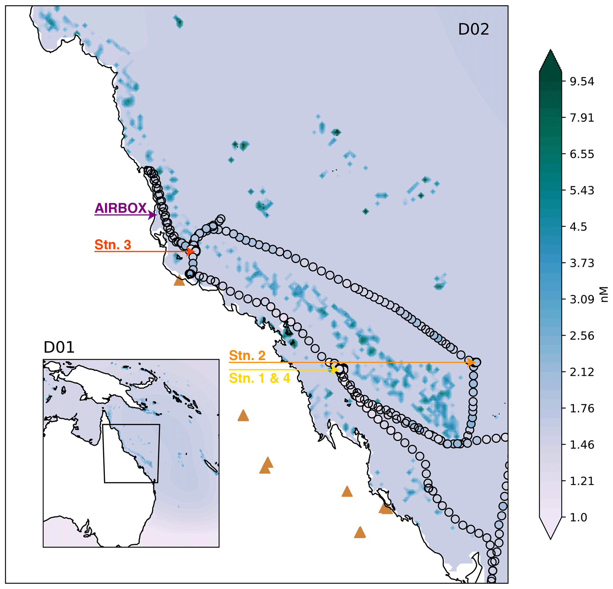
Figure 1Domain two (D02) of the WRF-Chem simulations, with the outer domain (D01) inset. The colours represent the DMS surface water concentrations for the simulations including coral-reef-derived DMS (note the log scale). The RVI ship track is shown by black outlined circles, also coloured by DMS observations. The locations of the RVI stations and AIRBOX are shown by coloured text and arrows. The brown triangles indicate where fossil fuel or biomass burning power generators are located.
2.2 DMS climatologies
The default DMSw climatology provided by WRF-Chem is the outdated Kettle and Andreae (2000) climatology on a 1 × 1.25∘ grid. The climatology used here is the updated Lana et al. (2011) DMSw (referred to henceforth as the L11 climatology), though we note that this has recently been updated again (Hulswar et al., 2021). The interpolation performed by WRF-Chem (via Prep-Chem) was deemed unsatisfactory (creating unphysical patterns around the coastlines and generally a very coarse interpolation). For this reason, the L11 climatology for October was interpolated to each WRF-Chem domain using the Python (v3.5) basemap bilinear interpolation, overriding the default WRF-Chem DMSw climatology. Further smoothing around the coastlines was performed. All fields that pass through Prep-Chem underwent the same interpolation to a higher resolution for consistency.
After initial testing, it was found that simulations using L11 overestimated DMSw in comparison to observations taken during the R2R campaign (this finding will be described in Sect. 3). For this reason, a scaled DMSw climatology was created, where L11 was divided by 2.8 to match the average DMSw observations taken during the R2R campaign. The scaled climatology is referred to as L11S henceforth.
To examine the impact of coral-reef-derived DMS, a new source of DMSw was added to the L11S climatology. The coral reef source was determined using the areal fraction of coral reefs per WRF-Chem grid box to add a weighted 50 nM of DMSw, matching that of the global analysis performed in Fiddes et al. (2021). The 50 nM value was chosen as a high range estimate in order to maximise any potential signal and response. In reality, this source varies considerably with time (e.g. up to as much as 54 nM; Jones et al., 2007) but is likely much smaller. The coral reef DMSw source added to the L11S climatology is referred to as L11SCR and is shown by the coloured contours in Fig. 1 alongside the R2R DMSw observations.
2.3 Experiment set-up
Three simulations are analysed in this study. The first simulation uses the L11 climatology (and hence will be referred to as the L11 simulation), with no biomass burning or dust and with the Gong et al. (1997) sea salt emissions. While this climatology is not the default DMSw climatology in WRF-Chem, it is the most up to date, warranting its evaluation. The second simulation uses the L11S DMSw climatology scaled to the ship observations (and subsequently referred to as the L11S simulation). In addition, L11S uses the Fuentes et al. (2010) sea salt parameterisation, which now includes an organic aerosol component that is excluded under the Gong et al. (1997) parameterisation. Biomass and dust emissions are also included. The third simulation uses the L11SCR DMSw climatology and otherwise the same set-up as L11S, to examine if coral-reef-derived DMSw plays a role in aerosol characteristics over the region.
2.4 Observations and evaluation methods
The 2016 major field campaign, R2R, aimed to determine if marine aerosol produced by the GBR could affect CCN concentrations, cloud formation and subsequently the hydrological cycle, providing essential observational evidence for assessing DMS–climate interaction. A leading motivation for this field campaign came from observations by Modini et al. (2009). A selection of the data from this campaign are used in this work to evaluate the WRF-Chem model.
The R2R field campaign took place on two platforms, the first on board the CSIRO Marine National Facility RV Investigator (RVI) which navigated a path around the GBR from 28 September–22 October 2016. The ship track is given in Fig. 1. The second platform used in R2R was the Atmospheric Integrated Research Facility for Boundaries and Oxidative Experiments (AIRBOX) mobile atmospheric chemistry lab, stationed at Mission Beach, QLD, from 20 September to 16 October 2016. The position of AIRBOX is given in Fig. 1. While a subset of AIRBOX data has been described previously in Chen et al. (2018) (including lidar, aerosol, trace gas and meteorology data), this is the first work to use the new data set from across the R2R campaign. However, we note that an overview paper on this campaign is currently in preparation (Trounce et al., 2022).
Observations collected both on the RVI and at AIRBOX comprised measurements of meteorology and atmospheric chemical and aerosol composition. These observations aimed to capture each step of the DMS cycle over the GBR for the first time. A list of observations used in this study from the R2R campaign can be found in Appendix B, Tables B1 and B2 as well as a brief description of how the data were collected and processed. All observations are available from the relevant institutions upon request.
To compare the estimated fluxDMS from the model and observations, we used the Liss and Merlivat (1986) parameterisation given modelled and observed DMSw, SSTs and wind fields. To evaluate sulfate aerosol, particle size bins were linearly interpolated to observed particle sizes, assuming aerosol bins are internally mixed. In order to determine periods of time in which the RVI observations were contaminated by ship exhaust, the hourly black carbon concentrations needed to be above 50 ng m−3, and the wind direction relative to the ship was >120 and <240∘. Any time stamp within ± 5 min of meeting these two criteria was also flagged. Air masses were considered to have marine origins if radon concentrations were below 300 mBq cm−3.
To aid the air mass characterisation, the Hybrid Single Particle Lagrangian Integrated Trajectory Model (HYSPLIT) was used to perform back trajectories (Draxler and Hess, 1997, 1998). The National Centers for Environmental Prediction (NCEP) Global Data Assimilation System (GDAS) 0.5∘ product was used to produce the back trajectories, where vertical motion was calculated using the model vertical velocity. Initial height was set at 100 m, and the trajectories were run for 72 h, every 2 h. Further characterisation of air masses has been performed by splitting WRF-Chem aerosol into boundary layer and free troposphere masses. The simulated boundary layer height was used. This was done to explore if any specific changes to aerosol could be found in either air mass, in particular due to the differing nucleation processes that occur at the two different levels, and following from Fiddes et al. (2018), who found some impact on nucleation rates in the free troposphere in response to perturbations of coral-reef-derived DMS.
For the WRF-Chem evaluation, time series comparisons, correlations and a bias factor metric have been used, evaluating equivalent model fields to the observations taken during R2R. For this work, evaluation is focused on the WRF-Chem domain two. We note that in both domains, WRF-Chem considers the AIRBOX grid point as ocean (the container was < 50 m from the shoreline). This has had some impact on how well the model captures the meteorology at AIRBOX (Fig. C2 in Appendix C). The normalised mean bias factor (NMBF; Yu et al., 2006) is used. The NMBF is a symmetric metric, i.e. negative biases are not bound by zero, and remains viable when measured values are much smaller than model values. This metric is an improvement on other model performance metrics, as described by Yu et al. (2006). To ensure clarity of this metric across both positive and negative biases, the NMBF has been converted into a bias factor (BF) by adding 1 if NMBF < 0 or subtracting 1 if NMBF > 1. Correlation analysis has been performed using Spearman's rank correlation methods (Wilks, 2011). This method is a non-parametric test that quantifies the monotonicity of the relationship between two variables.
3.1 Surface water DMS and the resulting sea–air flux
Figure 2 shows the time series of DMSw, wind speed and the resultant fluxDMS for the three WRF-Chem simulations and the RVI observations. In Fig. 2a, the effect of scaling the L11 DMSw climatology can clearly be seen, where L11S represents a more realistic value for the GBR region with a BF of 1.02 compared to L11 of 2.74. While the L11 climatology is, as of writing, the most up-to-date gridded data set of DMSw available, we can see that for this region it significantly overestimates DMS. This result highlights that much greater sampling of DMSw variability over space and time is required, especially in regional studies. We note a new DMSw climatology has just been submitted for review (Hulswar et al., 2021) and that Lana et al. (2011) is not the default climatology for WRF-Chem, rather the original Kettle et al. (1999) climatology.
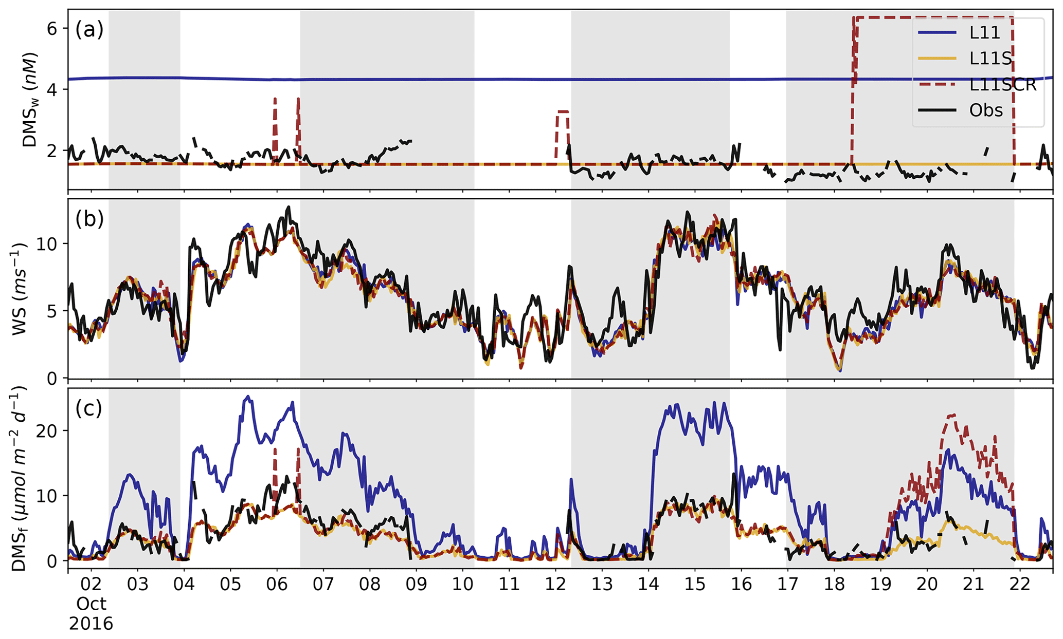
Figure 2RVI observations (black) and model estimates (coloured) of (a) DMSw (nM), (b) wind speed (m s−1) and (c) the fluxDMS (µmol m−2 d−1). Note the fluxDMS is calculated from observations using the Liss and Merlivat (1986) parameterisation. The three WRF-Chem simulations are L11 (blue), L11S (yellow) and L11SCR (dashed red). The grey shading from left to right indicates when the ship was at station locations 2, 3.1, 3.2 and 4.
Figure 2b shows that overall, the model predicts wind speed along the RVI path well, with L11S having a NMBF of 1.06 and a correlation coefficient of R=0.87 to the observations. The diurnal cycle is also well captured (not shown), although the model tends to underestimate and delay the peak wind speed. This is attributed to the poor simulation of the sea breeze structure (results not shown). Some model skill may be attributed to the fact that RVI observations are assimilated into the BARRA reanalysis product used to nudge the model, although we also note that model winds are free-running below 3 km. Comparison of wind roses (not shown) indicates that the model has a bias of winds from the south-east. This bias reflects the predominant large-scale flow over the area for this time of year. Generally, however, the model captures the overall meteorology as well as can be expected for the RVI (see Fig. C1) though less satisfactorily for AIRBOX (Fig. C2).
Wind speed is a key factor in the Liss and Merlivat (1986) flux parameterisation. An estimate of the fluxDMS along the RVI track is shown in Fig. 2c. Here we can see that despite the model's constant DMSw, it is able to do a comparatively good job representing the average fluxDMS, with a BF of 1.21 for L11S, compared to 2.32 for L11. This skill is predominantly due to the well-captured marine wind speeds discussed above. Visually, the L11S fluxDMS time series appears to follow that of the observations relatively closely although with a weak R value of 0.24 and underestimated variance (where σL11S=2.77, σObs=3.11), likely due to the constant DMSw.
From Fig. 2a, we can see where the ship is within a grid box that has an additional coral reef DMSw source included in L11SCR. The corresponding fluxDMS is in general much larger than what was observed, although we recognise that the ship did not measure directly over coral reefs. Nevertheless, this is a clear demonstration of how additional coral reef DMSw is influencing the fluxDMS and should subsequently influence DMSa.
3.2 Atmospheric DMS and sulfate aerosol mass
Figure 3a and c show DMSa from the RVI and at AIRBOX. The average at both sites is moderately well captured. For the RVI, the BF for L11S compared to the observations is 1.29, while at AIRBOX this is 1.42. Weak (negative) and insignificant correlations between the observations and simulations are found for both locations. The poorer performance of the model at AIRBOX may be due to the complexity of the location on the coast. However, the weak and negative correlations suggest that the model is missing an important aspect of DMSa variability, likely caused by the constant DMSw field or perhaps missing chemical sinks. While WRF-Chem has more complex DMS chemistry compared to other chemical models, comprising 30 DMS oxidation pathway reactions, it is possible that it is still missing important reactions. For example, the importance of DMS removal by BrO or Cl2 has been highlighted in the literature (Breider et al., 2010; Khan et al., 2016; Muñiz-Unamunzaga et al., 2018). Specifically, Khan et al. (2016) note that without these inclusions, the variability of DMSa is not well modelled.

Figure 3Observations (black) from the RVI (a, b) and AIRBOX (c, d) and corresponding model estimates (coloured) of (a, c) DMSa (ppb) and (b, d) aerosol mass (µg cm−3). The three WRF-Chem simulations are L11 (blue), L11S (yellow) and L11SCR (dashed red). The grey shading from left to right indicates when the ship was at station locations 2, 3.1, 3.2 and 4. Note that the dates in (a), (b) and (c), (d) are not the same.
Nevertheless, significant improvement can be seen in DMSa in the L11S simulations compared to the standard L11 simulation. The addition of coral reef DMSw has made a small difference in DMSa when near reef regions. However, the significant changes to DMSw between L11, L11S and L11SCR have not had a significant impact on the sulfate aerosol mass, shown in Fig. 3b and d.
For L11S, over the entire time series, the model underestimates the observations of sulfate aerosol mass by approximately 0.11 µg m−3, with a BF of 1.3. A moderate correlation of R=0.46 suggests that the model is capturing some of the observed trends and variability. For AIRBOX, the underestimation of the observations by L11 increases to 0.16 µg m−3, and the BF is 1.43. In addition, a statistically significant negative relationship is found between the two time series (). This is likely due to a number of local sulfate sources observed by AIRBOX that were not included in the model, for example, vehicle emissions, that impact the variability of the time series.
Importantly, we note that reducing DMSw by approximately 65 % between L11 and L11S results in a decrease of only 10 % in total surface sulfate aerosol mass along the RVI track. It is possible that this is because L11S also included biomass burning, while L11 did not. The mean difference of surface concentration for L11 and L11S over the entire RVI time series is −0.039 µg m−3. When periods of contaminated air (air masses that contained high levels of black carbon, had terrestrial influence or were flagged for other reasons) are filtered out of the calculations, the difference between L11 and L11S was −0.049 µg m−3, or a −15 % change. The difference between the filtered and unfiltered means suggests that the inclusion of biomass burning has offset the sulfate reduction caused by DMSw only marginally (by about 5 %). Nevertheless, these results imply that DMS only plays a small role in the sulfate aerosol burden over the GBR.
3.3 Terrestrial air mass influence
Figure 4a shows the time series of radon and black carbon (for both the RVI and L11S), the mean wind direction in the model and three sets of HYSPLIT trajectories over Stations 3.1, 3.2 and 4. It is clear from the radon time series that over the campaign, the ship did not encounter what could be considered clean marine air often (defined as periods below 300 mBq m−3), although we note that exposed coral reef atolls are also a source of radon. The radon time series is coloured by the exhaust contamination flag and indicates that there were even fewer occasions in which conditions uninfluenced by ship exhaust (shown by the green colours) or terrestrial air mass were measured.
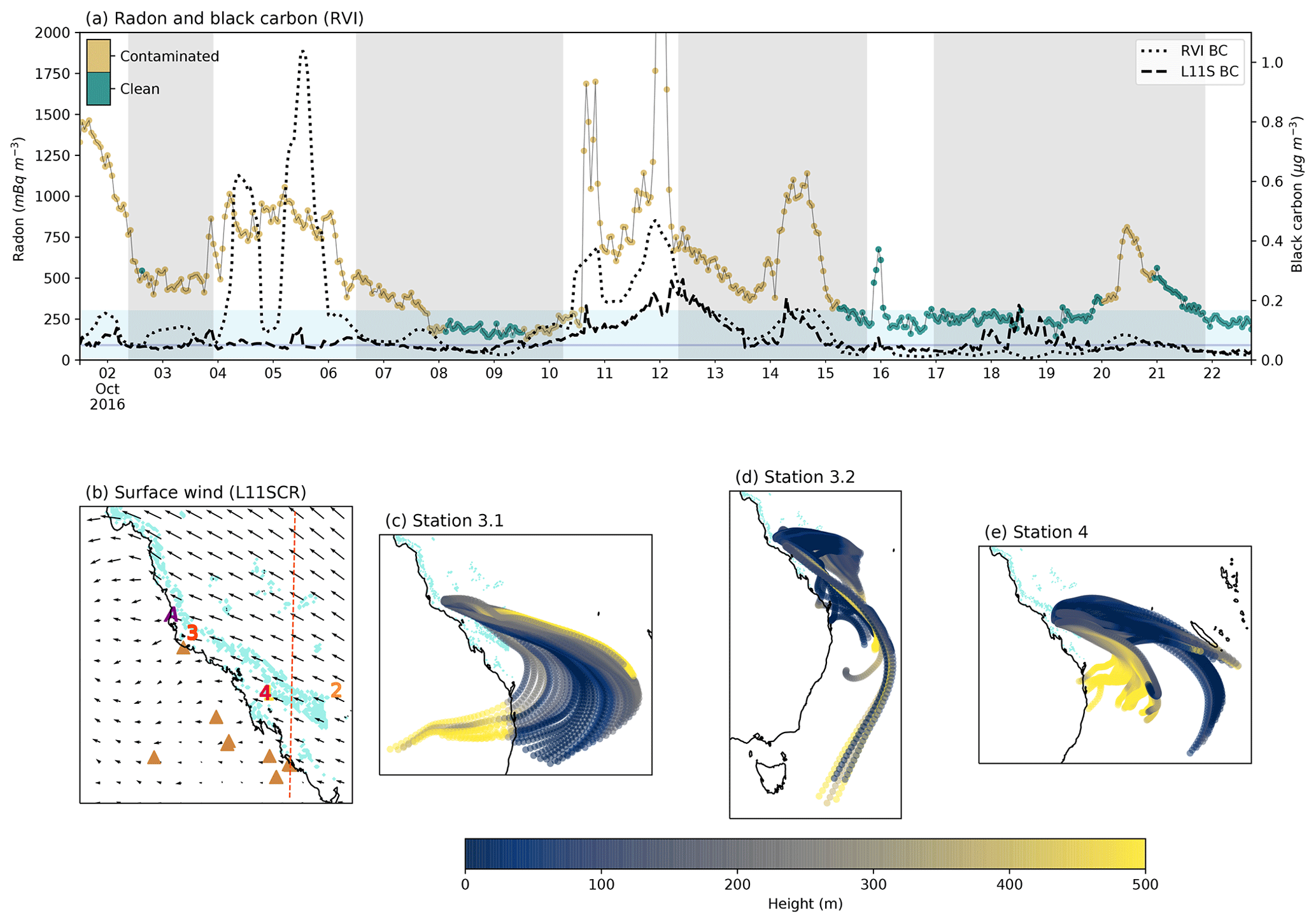
Figure 4(a) Radon concentrations from the RVI and coloured by the ship exhaust flag (left axis). Black carbon concentrations (right axis) from the RVI (dotted line) and L11S (dashed line). The light blue shading indicates when radon was below 300 mBq m−3, and the dark blue line indicates black carbon below 0.05 µg m−3. The grey shading represents ship stations 2, 3.1, 3.2 and 4. (b) the surface winds from L11SCR. Coral reefs are shown in light blue. Numbers indicate RVI observation stations 1–4 coloured yellow through to red, and the purple A indicates the AIRBOX location. The brown triangles indicate where fossil fuel power generators are located, and the dashed orange vertical line indicates where a transect was taken for vertical profile analysis. (c–e) HYSPLIT back trajectories for every 2 h while the ship was at station 3.1, 3.2 and 4 respectively, coloured by height.
Comparing the RVI black carbon to the L11S concentrations, where ship exhaust from the RVI is not included, we can see some agreement in periods of terrestrial air mass (e.g. between stations 3.1 and 3.2). While the L11S black carbon levels are lower than what was measured, the mean (in periods of no exhaust contamination) of 0.07 µg m−3 over the time period shown is above that of which was considered clean in this study (0.05 µg m−3), also implying a predominant terrestrial influence. We note that Fig. C4 shows an evaluation of BC at AIRBOX, where modelled BC is also lower than that of the observations (by a factor of approximately 3.3). The majority of this underestimation is due to some very large peaks in the observations which Chen et al. (2018) attributed in part to biomass burning but may also be a result of local vehicle movements. This may indicate that the model is not capturing some small-scale or transient terrestrial/anthropogenic emissions. This limitation is not detrimental to the results.
In Fig. 4b, south-easterly surface winds are shown to prevail, although some bias in the day-to-day wind direction was found compared to the RVI (see Fig. C1). Looking at this map, one may expect that this period did comprise clean marine air masses, and, as an example, this time of year was in part chosen due to this prevailing wind direction. However, as the 72 h HYSPLIT back trajectories in Fig. 4c–e show, despite the wind coming from the south-east, much of the time, this air mass had actually recirculated over the Australian continent and spent only a partial time over the ocean. The dominance of terrestrial air mass during the R2R campaign was also demonstrated by Chen et al. (2019), where much of the air mass measured at AIRBOX had strong terrestrial influence, with signatures of biomass burning.
In addition to unfavourable synoptic conditions, one such cause of a lack of clean marine periods is the influence of sea–land breeze coupling. Over coastal–marine regions, recycling of air masses over the land and ocean can occur and have far-reaching impacts. For example, a sea–land breeze circulation up to 150 km offshore under favourable conditions during the R2R campaign was detected in previous (unpublished) WRF simulations (Claire Vincent, personal communication, 2019). Similarly, sea–land coupling was also observed at AIRBOX (not shown). This circulation between land and ocean can lead to terrestrial air masses extending far offshore.
3.4 Dominant anthropogenic sources of sulfur
Now we consider not just how DMS has changed in response to the simulated coral reef perturbations over the RVI track or at AIRBOX but how it has changed over the entire WRF domain, and in particular over coral reef regions. To be clear, the changes in DMS are simulated only – not observed changes. A vertical transect of DMSa and the surface mean for the entire domain is shown in Fig. 5a and b. In this figure, the source of coral reef DMSa is clearly evident in the (simulated) boundary layer (panel c) and is blown with the prevailing model winds at the surface in panel (d). Over the entire domain, at the surface, a significant increase in DMSa of 0.003 ppb is found, approximately 12 %, with a mean increase of 40 % found over coral reef grid points. These significant increases in DMSa, however, do not result in significant change in sulfate aerosol mass, as found along the RVI track and at AIRBOX.
We note that the model captures the boundary layer height along the RVI track relatively well (Fig. C1), with some exceptions due in part to the model and in part to the physical limitation of the lidar system resulting in no boundary layer height detection below 500 m altitude, as well as possible misidentification of some cloud layers by the lidar algorithm (e.g. spikes in boundary layer height in the early time series). At AIRBOX, the boundary layer height is not as well captured (Fig. C2), in agreement with Chen et al. (2019). This result also agrees with previous work that indicates the Mellor–Yamada–Janjić (MYJ) boundary layer scheme underestimates the boundary layer height the most in coastal marine areas, which then improves further offshore (Rahn and Garreaud, 2010).
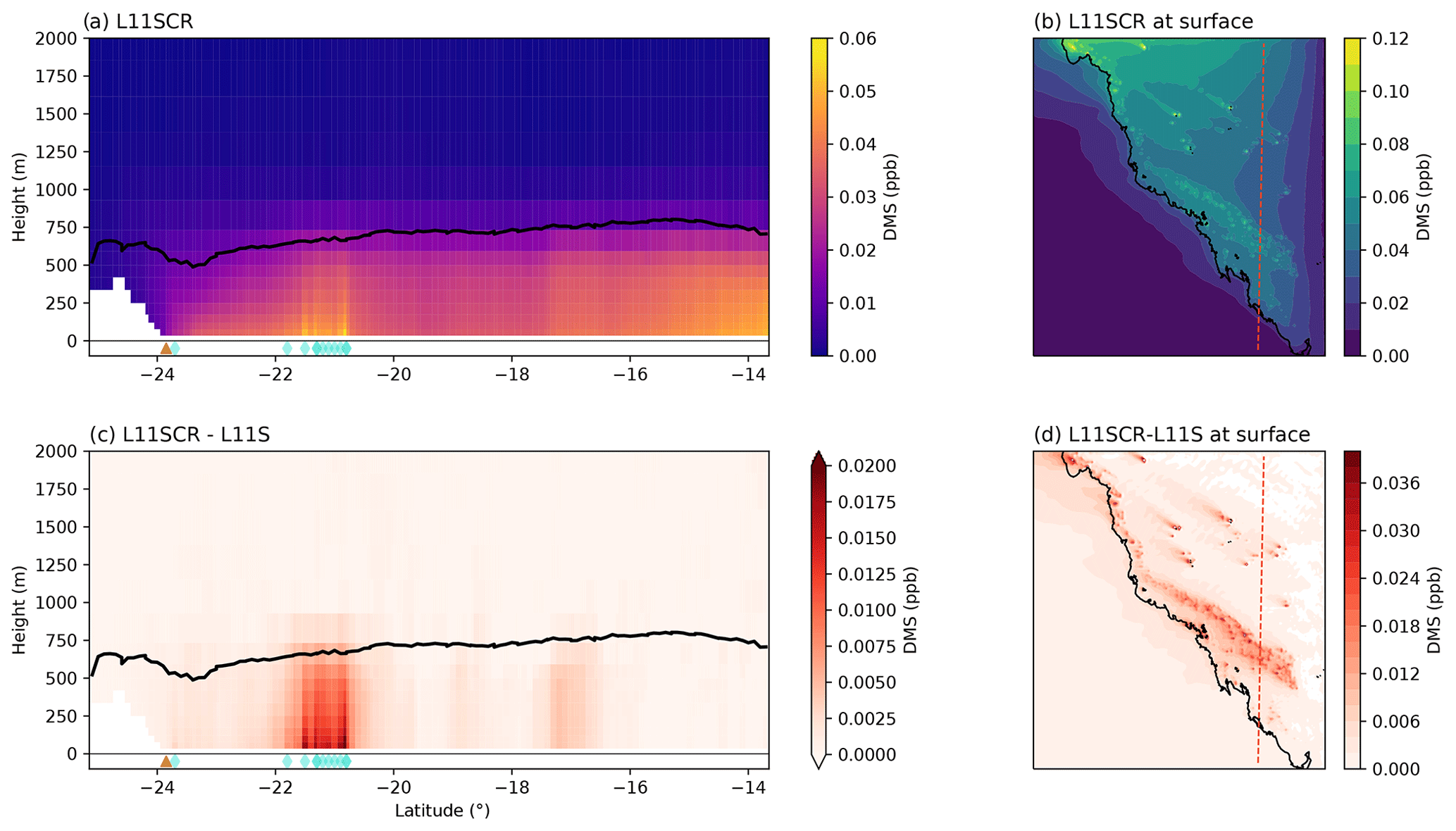
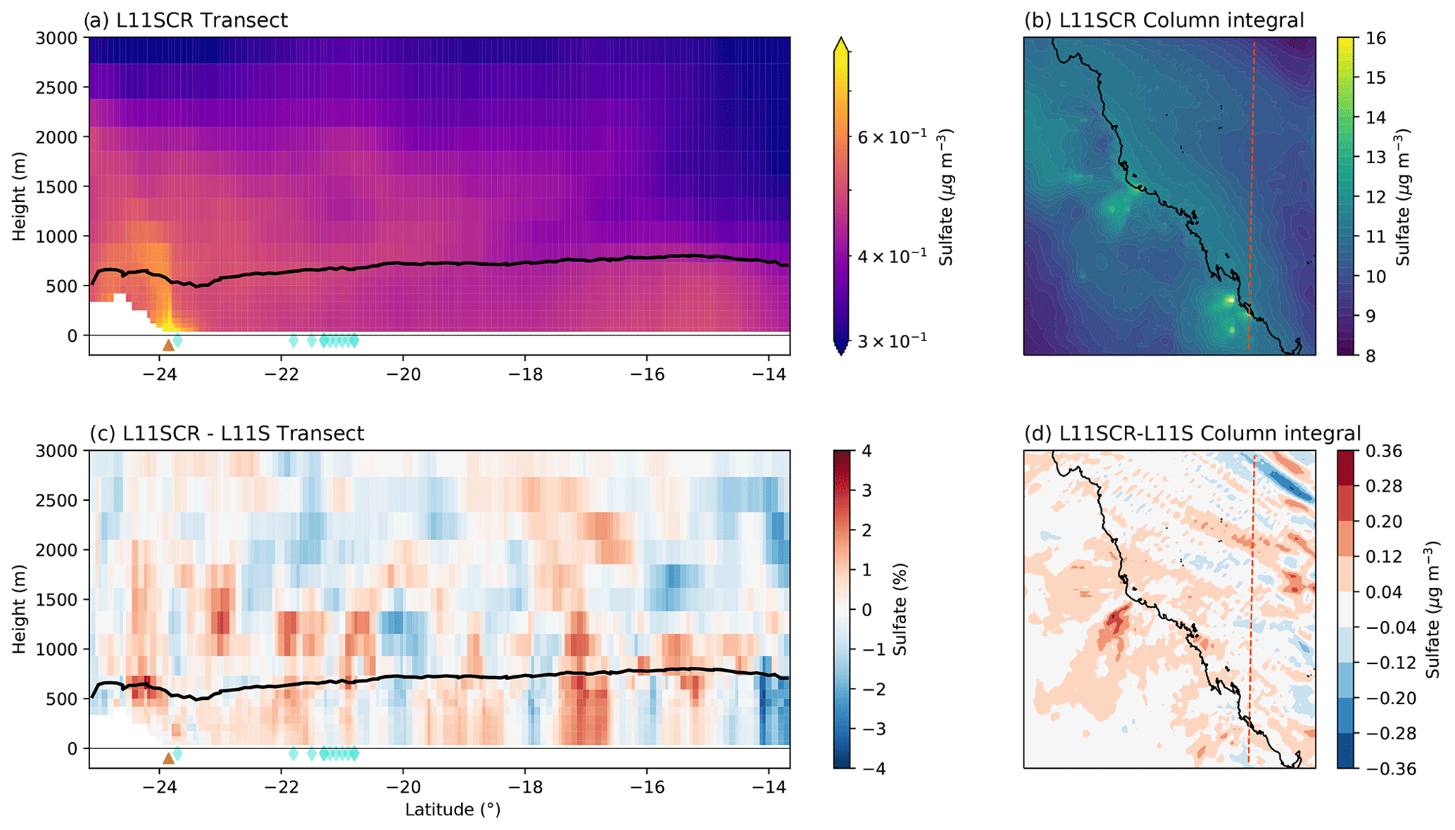
Figure 5Vertical transects (a, c) and surface means (b, d) of DMSa for L11SCR (a, b) and the difference between L11SCR and L11S (c, d). In (a) and (c), the black line indicates the mean simulated boundary layer height, while the brown triangle shows the location of the Gladstone power station, and the blue diamonds show grid points within which coral reefs are found.
Figure 6a and b show the vertical transect and surface mean of total sulfate aerosol mass (including in-cloud sulfate aerosol). These two plots clearly demonstrate that anthropogenic emissions represent a significant source of sulfate aerosol (among other species) for the GBR region. In Fig. 6a, over the Gladstone coal fire power station (brown triangle), a dominant plume in sulfate aerosol can be seen, while in Fig. 6b, numerous plumes, that align with known power generators, can be seen. We note that the same delineation between the boundary layer and free troposphere found in the DMSa plots is not seen in the sulfate aerosol mass.
Figure 6c and d indicate no coherent change in total sulfate aerosol mass that could be robustly attributed to the inclusion of coral-reef-derived DMS. The surface mean change between L11S and L11SCR over the entire domain is 0.0018 µg m−3, or a change of 0.38 %. Directly over coral reef grid points, an increase of 0.47 % was found.
3.5 Nucleation pathways of coral-reef-derived DMS
The prevalence of anthropogenic sulfur and the abundance of pre-existing particles suggest that the small addition of sulfate from DMS is unlikely to participate in new particle formation in the boundary layer. Rather, it is more likely that coral-reef-derived H2SO4 would condense onto pre-existing particles, growing their mass. Below, we analyse column integrals of aerosol number and mass in the free troposphere and boundary layer to test this hypothesis. We have separated the two atmospheric profiles as Fiddes et al. (2021) noted larger changes in the free troposphere in response to perturbed coral reef DMS than in the boundary layer.
Figure 7 shows the transect of the boundary layer (left) and free troposphere (right) total column sulfate mass and aerosol number for the bins representing Aitken- and accumulation-mode aerosol. We suggest that regions where the changes along the transects in the number and mass co-vary are likely due to internal model variability (e.g. some variation between model simulations independent of perturbations, despite the nudging, is expected), rather than changes in the DMSa field. In the larger bins (Fig. 7e–j), this appears to be the case in most locations. However, in the smaller bins (Fig. 7a–d), some instances where the mass has changed independently of the number are found.
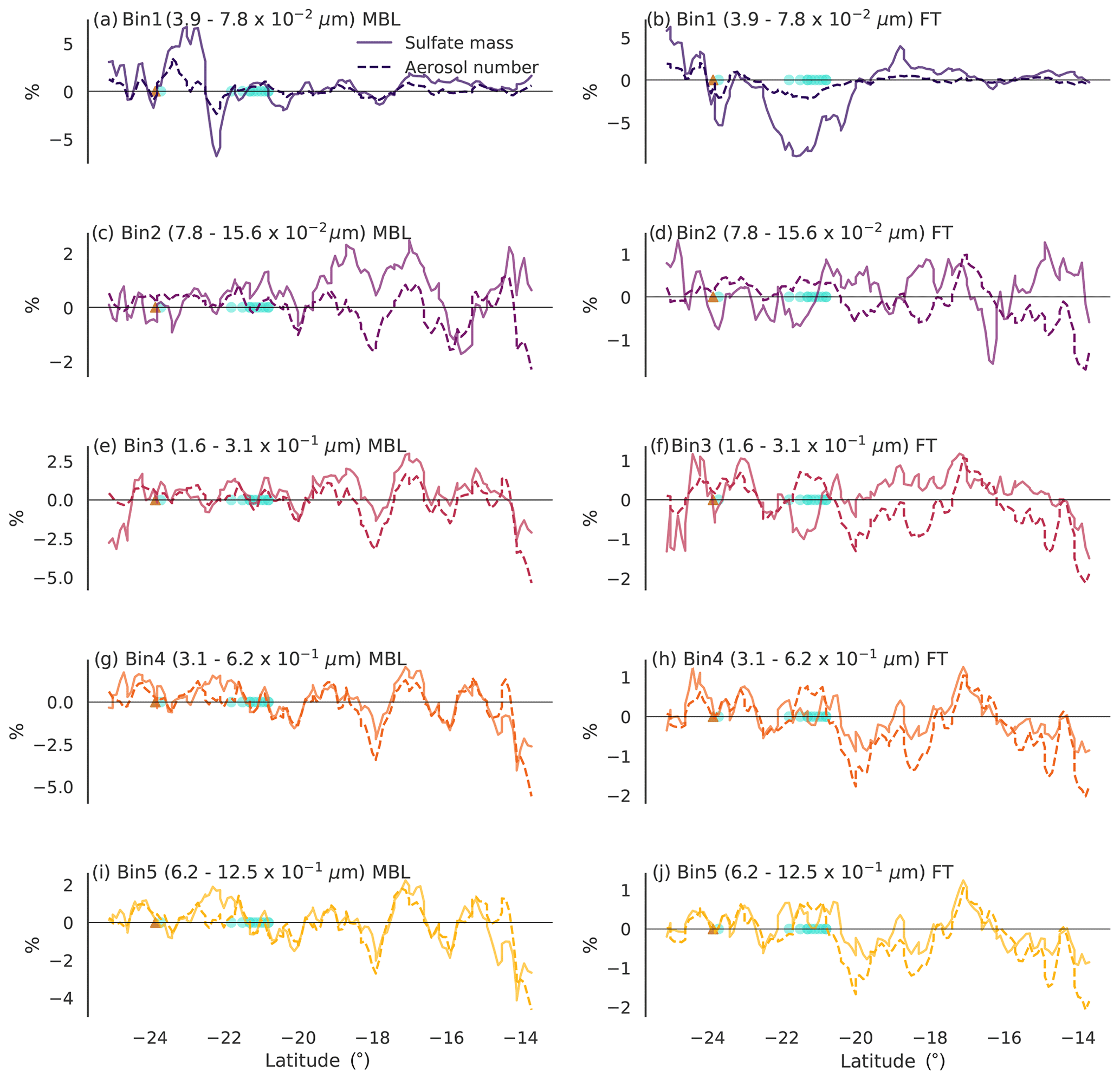
Figure 7Percentage changes (L11SCR-L11S) along the vertical transect of total boundary layer column (a, c, e, g, i) and free troposphere column (b, d, f, h, j) sulfate mass (solid line) and total aerosol number (dashed line) for the five smallest bin sizes representing the Aitken mode (bin 1) and accumulation mode (bins 2–5). The brown triangle shows the location of the Gladstone power station, and the blue circles show grid points within which coral reefs are found.
In Fig. 7a and c, the total boundary layer total column sulfate mass has increased in some areas, while the number has not. These increases may be evidence of condensational growth. Importantly, we note that the regions over which the increase in mass occur are not co-located with coral reefs but may be due to advected DMSa and its oxidation products.
In the free troposphere, new particle formation is far more likely to occur. Examining the smallest bin size (Fig. 7b), however, no clear evidence of the coral-reef-derived sulfuric acid participating in new particle formation is found. Rather, directly over coral reefs, a relatively large decrease in sulfate aerosol mass is found compared to the simulation without coral-reef-derived DMS, with a lesser reduction in particle number concentration. These decreases may suggest that the coral-reef-derived precursors have grown existing small-sized particles, causing them to shift into larger bin sizes. On average, over the transects for the remaining bin sizes, increases in free tropospheric sulfate mass were found, accompanied by decreases in number (keeping in mind that these changes are insignificant and less than 1 %). This may further suggest greater coagulation rates, reducing the number while increasing the mass. However, due to the very small and insignificant changes found, we have low confidence that these results are caused directly by coral-reef-derived DMS as opposed to model noise.
While locally, changes in sulfate mass in some cases appear to be up to 5 %, on average, the changes over the transects in either the boundary layer or free troposphere are less than 1 %. Furthermore, the largest signals from coral-reef-derived DMS appear to occur in the smallest size aerosol, with little discernible change in the larger aerosol sizes that are of greater climatic relevance. Examination of changes in cloud condensation nuclei (CCN, not shown) confirms this and indicates that the very small addition of sulfate by corals is unlikely to have any direct or indirect aerosol effects over the GBR region. Further investigation of these aerosol effects has been carried out (not shown), and no significant changes in clear sky radiation, total radiation, cloud droplet number, liquid water path, cloud fraction or precipitation were found.
An important limitation of this present study is the choice of model set-up in relation to the aerosol size distribution. In this work, the default aerosol size bins were used, which range from ∼39 nm to 10 µm (Fast et al., 2006), capturing aerosol in the Aitken mode through to the coarse mode. This set-up does not explicitly represent nucleation-mode aerosol, which is instead parameterised to contribute directly to Aitken mode via growth. The parameterisation of nucleation-mode particles will be discussed in greater detail below and is described in Appendix A. A model set-up in which the nucleation mode was explicitly resolved was not used in the present study as we followed the model set-up of Yang et al. (2011) and Saide et al. (2012), one of the few studies in the literature using WRF-Chem to examine the role of DMS in climate.
The impact of the nucleation-mode configuration on the results of this study could be twofold. Firstly, Lee et al. (2013) demonstrated that not explicitly including nucleation and early growth (including coagulation) of nucleation-mode particles can significantly overestimate the N10 (number of particles with a dry diameter greater than 10 nm). However, only minor impacts on CCN and the subsequent indirect aerosol effects were found when nucleation-mode processes below 10 nm were explicitly resolved. Such results have not been discussed in detail in this study, but we can briefly confirm that total aerosol number concentrations (N10 and CCN) were overestimated for this work (see Figs. C3 and C4).
In our previous work (Fiddes et al., 2021), the GLObal Model of Aerosol Processes (GLOMAP)-mode aerosol scheme was used, which explicitly included nucleation-mode aerosol below 5 nm. New particular formation was parameterised via the Kulmala et al. (1998) scheme in the free troposphere and organic mediated (Metzger et al., 2010) boundary layer nucleation scheme. In that work, a small impact on nucleation–Aitken-mode aerosol was found when coral-reef-derived aerosol was included, but these increases were not large enough to conclusively be found to have altered the CCN. It was also found that the largest differences in particles with a dry diameter greater than 3 nm were in the free troposphere. This present work, using the same coral-reef-derived DMS contributions, also found a small change in Aitken-mode aerosol and little to no change in CCN. A fully resolved nucleation mode may result in fewer ultra-fine (below 70 nm) aerosols and change how coral-reef-derived aerosol may interact with the ambient aerosol burden. However, in light of our previous work, we do not have reason to believe that the conclusions of this work would be significantly altered for the present-day climate.
Secondly, a number of studies have reported the impact of including new particle formation on clouds and radiation, where new particle formation increases the condensation sink (Blichner et al., 2021) and reduces the amount of sulfuric acid available for condensation (Sullivan et al., 2018), resulting in inhibited growth of particles into CCN, thereby reducing the cloud albedo. This mechanism is further supported by Gordon et al. (2016), where, under pre-industrial conditions, the inclusion of biogenic new particle formation results in large decreases in cloud albedo. Blichner et al. (2021) also find that under present-day conditions, new particle formation, including early growth, has a greater influence on the activation of cloud droplets than under pre-industrial conditions, in part due to the increased sulfate burdens and associated increased hygroscopicity, resulting in CCN activation at smaller sizes.
In this work, no discernible effect was found on cloud or radiative properties. Whether this is caused by the model set-up or is because the coral-reef-derived source of aerosol is insignificant is difficult to conclude in this study alone. However, Fiddes et al. (2021) also found little to no effect on cloud radiative properties, indicating that the results here are robust.
In addition to the limited aerosol bin sizes discussed above, the choice of nucleation mechanism, whether parameterised or more fully resolved, is likely of some importance to this work. Much community effort has been undertaken to improve our understanding of new particle formation, including new observations, as well as updated parameterisations (Lee et al., 2019; Semeniuk and Dastoor, 2018). Here, the Wexler et al. (1994) parameterisation is used, in which only binary nucleation of sulfuric acid with water is included. Current understanding suggests that binary nucleation cannot satisfactorily parameterise sulfate concentrations in the clean marine boundary layer (Semeniuk and Dastoor, 2018). To add to this, ternary nucleation processes (with ammonia) have been found to under-predict new particle formation (Semeniuk and Dastoor, 2018; Zaveri et al., 2008).
These findings demonstrate how complex new particle formation is and how much we still need to understand. For example, literature suggests that nucleation involving amines, ammonia, iodine or other ions with DMS or MSA may be important for coastal regions, such as Mace Head or the Antarctic Peninsula (Brean et al., 2021; O'Dowd et al., 2002; Semeniuk and Dastoor, 2018). Other work has suggested that the presence of isoprene, a compound emitted in large quantities by eucalypt forests (Emmerson et al., 2020), may suppress new particle formation (Lee et al., 2019). How important these compounds and interactions are for the GBR, a tropical coastal marine region bounded by significant eucalypt forests, has not been quantified. While these processes are not included in our work, we hope that this present study can be used as a beginning point to understand the aerosol processes of the region more fully.
In summary, a more representative aerosol scheme is desirable, in particular to better understand the possibility/influence of boundary layer nucleation, as suggested to be possible by Modini et al. (2009). Though the set-up of the current work may have precluded the ability of boundary layer nucleation to realistically occur, our previous work suggests that nucleation in the free troposphere is more important, and hence we do not expect significantly different results. Nevertheless, we strongly recommend any future work similar to the present study employs a more fully resolved size distribution similar to Matsui et al. (2011), Zhao et al. (2020) or Sullivan et al. (2018) within WRF-Chem or uses alternate regional models such as in Gordon et al. (2018) and, if available, a nucleation mechanism that considers the complexity of a coastal marine environment.
Finally, further limitations of this study include the nudged meteorology (every 6 h), potentially limiting the ability of indirect aerosol effects to occur and any possible feedbacks. As shown in Fiddes et al. (2021), large differences can be found in aerosol–climate processes between nudged and free-running simulations, although differentiating between model noise and a real signal is difficult. However, we do not expect that in a similar free-running study the results would be significantly changed due to the very small changes in aerosol found in this work, the abundance of anthropogenic aerosol and the fact that the meteorological nudging was not applied in the boundary layer. Furthermore, the 4 d restarts of WRF-Chem, despite ingesting the previous day's chemistry, appeared to impact total aerosol numbers, including CCN, which were found to be strongly constrained by this set-up choice. This impact has limited the analysis of these fields in this study. The restarts were not thought to impact the DMS processes, in part due to the lifetime of DMS in the atmosphere.
Coral reefs as an unaccounted for source of DMS have gained attention over recent years, with numerous observational studies suggesting they play an important and even regulatory role in local climate (Jones, 2013; Hopkins et al., 2016; Jones et al., 2017; Cropp et al., 2018; Jackson et al., 2018, 2020b). While Fiddes et al. (2021) in a global modelling study found that coral-reef-derived DMS over the Maritime Continent and Australian region had little impact on long-term climate, no regional-scale modelling has been performed prior to this present study. This is particularly important if we are considering temporal and spatial resolutions relevant to bioregulatory feedbacks. In this work, we have evaluated the ability of WRF-Chem to simulate DMS and sulfur processes and tested the sensitivity of these processes to perturbations in DMSw, with a particular focus on coral-reef-derived DMS.
We find that, compared to observations taken during the R2R campaign, the Lana et al. (2011) climatology significantly overestimates DMSw and required reduction by 65 % to be of a similar magnitude. This finding adds to a growing argument of a need for an updated and, if possible, time-varying (beyond the fixed monthly climatology) DMSw climatology (e.g. as suggested in Green and Hatton, 2014). We note that a third-generation climatology has recently been developed (Hulswar et al., 2021); however this still does not address the need for time-varying data sets. Furthermore, our finding demonstrates that greater attention needs to be paid to the DMSw climatology within modelling systems, highlighted by the fact that the default WRF-Chem climatology is the out-of-date Kettle and Andreae (2000) climatology.
With a DMSw field that aligns with observations, the Liss and Merlivat (1986) fluxDMS calculated from both observations and the model agrees reasonably well in magnitude. This result is in part due to the well-captured marine wind speeds along the RVI track. Subsequently, DMSa is also reasonably well captured, although overestimated, as is sulfate aerosol mass over the ship track. The Liss and Merlivat (1986) flux parameterisation is considered a conservative parameterisation compared to other methods which provide much larger fluxes (see Appendix for details). Hence the overestimation of DMSa found here (despite matched DMSw and well-captured wind speeds) further suggests that Liss and Merlivat (1986) is the most realistic parameterisation for calculating the fluxDMS. Nevertheless, this evaluation gives us confidence that the model is able to capture the key processes in the DMS–aerosol system.
By comparing simulations with the original Lana et al. (2011) DMSw climatology to the scaled climatology, we find that DMS plays only a small role in sulfate aerosol burdens over the GBR. For a 65 % reduction in DMSw, a subsequent 67 % reduction in DMSa and a 10 %–15 % reduction in sulfate aerosol mass were found at the surface. Examination of the background meteorological conditions indicates that influence from terrestrial air masses occurred for the majority of the R2R campaign, which was broadly reflected in the WRF-Chem model. Furthermore, we suggest that local anthropogenic sources of sulfur from fossil fuel power generation are likely to have a strong influence over the GBR air mass due to proximity, interaction of the sea breeze and synoptic conditions. We recommend further observational studies are carried out to confirm if this is the case for different times of year. Additionally, we note that major coral bleaching events occurred in the summer prior to this field campaign. While the coral reefs south of Cairns (the region of this campaign) were not as severely bleached, we cannot rule out an impact on the production of DMS by coral reefs due to this event.
These results suggest that much smaller changes in DMS from coral reefs are unlikely to have a large impact on the aerosol burden. We find that by adding in a source of coral reef DMS, the total sulfate aerosol mass increases by less than 1 %, while insignificant changes of a similar magnitude were found for the total aerosol number. Over the time period studied, no evidence of new particle formation was found, although condensational growth in boundary layer and free troposphere in the smallest aerosol bins may have occurred. No evidence of direct or indirect aerosol effects was found in response to these very small changes in aerosol mass and number.
Whether the lack of influence from coral-reef-derived DMS on the local aerosol burden was a result of unfavourable synoptic conditions or model limitations is difficult to assess. However, the close proximity of anthropogenic aerosol emissions to the inner GBR suggests that this region should not be considered a “clean marine” environment unless under very specific conditions, therefore limiting the role that coral-reef-derived DMS can play in aerosol formation and growth while these emissions continue. We suggest that the influence of anthropogenic aerosol is analysed in future work by exploring if an increase in ammonium was also found, associated with sulfate produced by a power station. While Modini et al. (2009) suggested that they had observed new particle formation in such clean marine conditions, further work needs to be done to understand how often such conditions occur over the GBR before we can consider if these new particle formation events could have an influence on aerosol and weather.
This study indicates that it is more likely the small contribution of volatile sulfur compounds from the GBR contributes to aerosol growth via condensational pathways. While this is in agreement with the hypothesis presented in Jackson et al. (2020b), our results suggest that the growth in the smaller sized aerosol (Aitken mode) due to coral-reef-derived DMS is still too small to have an impact on radiative or cloud processes. This finding is in agreement with the global simulation study described in Fiddes et al. (2021). We suggest future work focuses on what the influence of coral-reef-derived DMS may be under “pristine” conditions. Planned work will target the clean marine period identified in the R2R campaign and consider the downwind processes from the RVI to AIRBOX, where the air mass crosses coral reefs. As this work has shown, small increases in sulfate aerosol mass are found directly over coral reefs, and how this evolves downwind is of interest. Modelling studies that test the sensitivity of influence of coral-reef-derived DMS to other aerosol burdens (e.g. anthropogenic, biomass burning or sea spray) would also be of significant value. Of further interest, and perhaps yielding more significant results, would be a study conducted under pre- or post-industrial emissions conditions. Simulations such as this become particularly relevant if we consider a post-anthropogenic aerosol emissions world, in which coral reefs such as the Great Barrier Reef may already be extinct.
A1 Chemistry and aerosol
The Carbon Bond Mechanism Z (CBMZ) chemical mechanism with aqueous chemistry and DMS is used in conjunction with the Model for Simulating Aerosol Interactions and Chemistry (MOSAIC) aerosol scheme. Dry deposition of gases and aerosol is turned on, as is wet scavenging (including convective wet scavenging). In-cloud chemistry, turbulent mixing and subgrid convective transport are also switched on. The FTUV (fast Tropospheric Ultraviolet-Visible) photolysis scheme (Tie, 2003) is used.
MOSAIC represents aerosol via a sectional approach with eight discrete size bins. For each bin, the number and mass of particles are simulated: defined by the lower and upper limit of the dry particle diameter (Zaveri et al., 2008). Particle growth is calculated in a Lagrangian manner, and transfer of particles between bins is calculated using a two-moment approach (Simmel and Wurzler, 2006). Coagulation of aerosol is calculated according to Jacobson et al. (1994). Homogeneous nucleation of H2SO4–H2O in MOSAIC is calculated via the Wexler et al. (1994) scheme. In MOSAIC, growth to Aitken-mode particles (the smallest bin size in this simulation) is simulated implicitly as newly nucleated particle sizes are smaller than the smallest simulated aerosol size in the model. Heterogeneous nucleation in MOSAIC is partitioned into two schemes, treating condensation of non-volatile gases (H2SO4 and methanesulfonic acid) and condensation and evaporation of semi-volatile gases (HNO3, HCl and NH3) separately (Zaveri et al., 2008).
MOSAIC includes 11 specific aerosol species, sulfate ( and ), methanesulfonate, nitrate, chloride, carbonate, ammonium, sodium, calcium, black carbon, primary organic matter plus water, and treats other unspecified aerosol species as a lumped mass or through substitutions of equivalent species. Some gas-phase species, including sulfuric acid and MSA, are allowed to partition to the particle phase. Atmospheric DMS chemistry is not a part of the CBMZ scheme but was added with the development and coupling of MOSAIC (Zaveri et al., 2008). The DMS chemistry is based on that of Zaveri (1997) and includes 11 species and 30 reactions.
The Liss and Merlivat (1986) parameterisation is used to calculate the fluxDMS emissions in WRF-Chem. As noted in Fiddes et al. (2018, 2021), the Liss and Merlivat (1986) parameterisation is considered a conservative method but is believed to be the most realistic (Vlahos and Monahan, 2009; Bell et al., 2017). Sea salt emissions are calculated online via either the Gong et al. (1997) parameterisation or the Fuentes et al. (2010) adaptation, which includes a large addition of marine organic matter. All sea salt schemes have been found to overestimate sea salt emissions in WRF-Chem (e.g. in Saide et al., 2012) and the Fuentes method especially so. Hence for simulations using the Fuentes high-organics option, the sea salt emission was halved, as was the sea salt mass within the boundary and initial conditions.
Dust emissions are calculated via the Shao et al. (2011) scheme. Wet deposition of dust has been turned on and follows the Jung and Shao (2006) method. For daily biomass burning emissions, fire location data are provided by FIRMS (Fire Information for Resource Management System) via the MODIS (Moderate Resolution Imaging Spectroradiometer) Collection 6 platform operated by NASA and available from https://earthdata.nasa.gov/firms (last access: 11 February 2022). The Brazilian Biomass Burning Emission Model (Longo et al., 2010) calculates the respective emissions and plume rise at daily resolution. Biogenic emissions are calculated online using the Guenther scheme (Guenther et al., 1994; Simpson et al., 1995). Anthropogenic emissions are prescribed from the Emissions Database for Global Atmospheric Research (EDGAR) V4.2, available at https://edgar.jrc.ec.europa.eu/ (last access: 11 February 2022) (European Commission Joint Research Centre and Netherlands Environmental Assessment Agency, 2012). Aircraft and volcanic emissions are not included.
A2 Physics
All simulations use the Morrison double-moment cloud microphysics scheme (Morrison et al., 2008). The RRTMG (Rapid Radiative Transfer Model for general circulation models) for longwave and shortwave radiation is used (Iacono et al., 2008), including the Monte Carlo Independent Column Approximation method for random cloud overlap (Barker et al., 2003). Cumulus parameterisation was performed using the Grell 3D scheme, similar to the Grell–Devenyi ensemble scheme (Grell and Dévényi, 2002). In addition, cumulus radiation effects are switched on, allowing for interaction of the radiation scheme and parameterised convective clouds (Gustafson et al., 2007). Cloud fractions are calculated using the Xu and Randall (1996) method, while cumulus and aerosol radiative feedbacks are permitted. Aerosol optical properties (Mie calculations) are approximated using the volume averaging method. The Noah land surface model is used, with soil temperature and moisture in four layers, fractional snow cover and frozen soil physics (Chen and Dudhia, 2002). The boundary layer scheme used is the Mellor–Yamada–Janjić scheme (Janjić, 1994) operating in conjunction with the surface layer physics scheme, Eta (Janjić, 1996).
In WRF-Chem, with the chemistry and physics options described above, aerosol direct and indirect effects are permitted via the radiative, photolysis and cloud microphysical schemes. For direct aerosol effects, the size, number and composition of aerosol and aerosol water, refractive indices of aerosol types (based on literature) and the Mie calculations (Bohren and Huffman, 1998) update the AOD, the single-scattering albedo and the asymmetry factor used in the RRTMG radiation scheme. Aerosol water has a large impact, and hence the relative humidity must also be considered when direct effects are being examined. In this work, water vapour has been nudged to the BARRA reanalysis and hence should not change significantly between experiments.
For indirect aerosol effects, the CCN number and composition are used to calculate the cloud droplet number (CDN) in aerosol activation modules (Abdul-Razzak and Ghan, 2000, 2002). Activation depends on the composition and size of the particle (i.e. their hygroscopic properties), as well as the vertical and turbulent velocities of the air mass. For the first indirect effect, CDN and the cloud water mixing ratio are used to calculate the cloud particle size and effective radius, which then inform the calculation of cloud albedo. The second indirect effect is simulated within the cloud physics routines (Morrison et al., 2008), which are informed by the CDN, and subsequently updates the autoconversion rate, rain mixing ratio and precipitation of the module. Lastly, for the semi-direct effect, the cloud optical properties are influenced by the absorption of solar ultraviolet and infrared fluxes altering the heating rate of cloud liquid water. It must be noted that the indirect effects can only be simulated via the microphysics, and hence at non-cloud-resolving scales, care must be taken in the interpretation.
Table B1List of RVI observations used in the WRF-Chem evaluation, the institute responsible for data collection and processing, details on the instrument used and literature relevant to the data processing methods
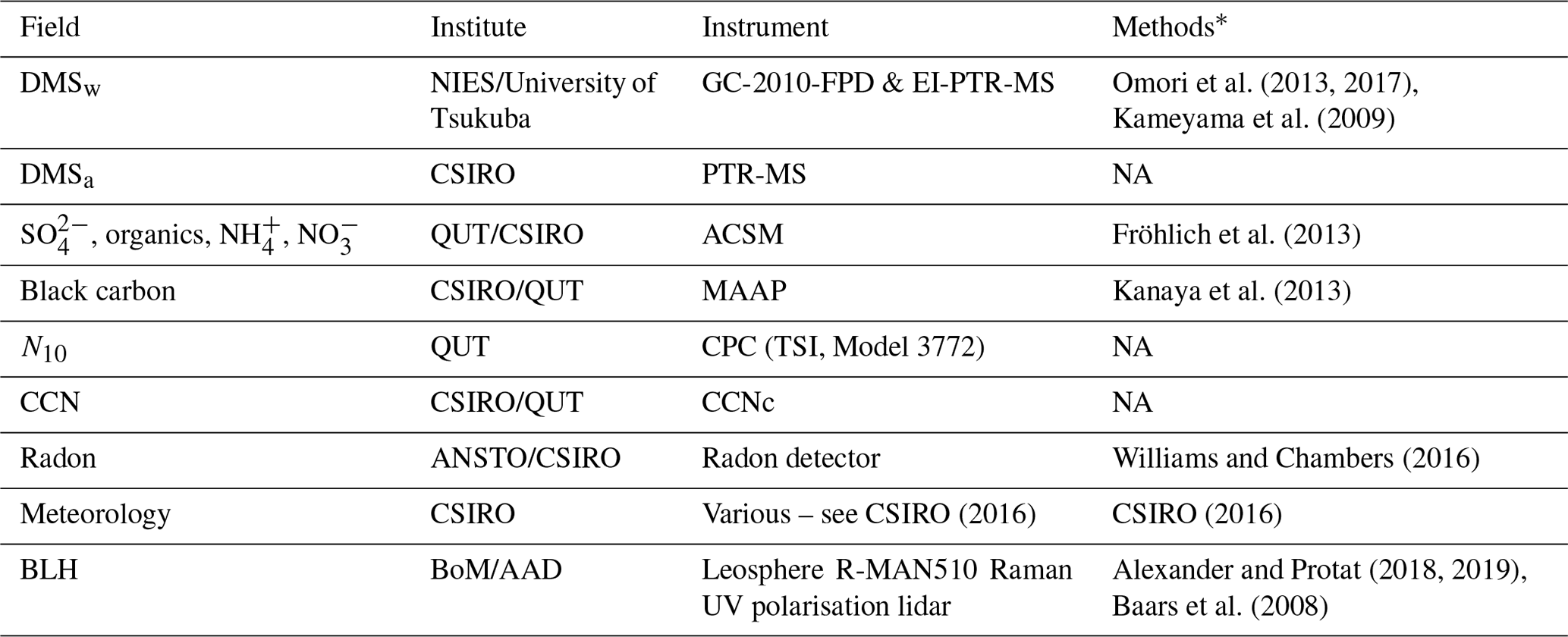
* Refer to in-text data description for full methods. NA – not available.
Table B2List of RVI observations used in the WRF-Chem evaluation, the institute responsible for data collection and processing, details on the instrument used and literature relevant to the data processing methods
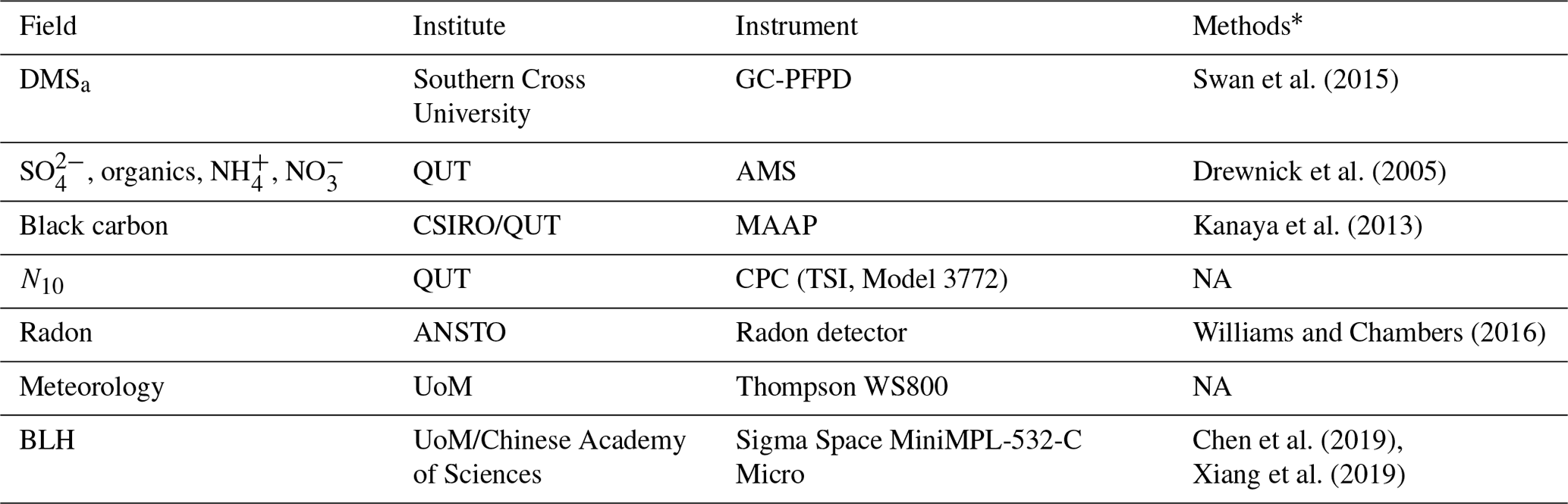
* Refer to in-text data description for full methods. NA – not available.
B1 DMS fields
DMSw observations were taken by the RVI for the duration of the voyage. Seawater samples (from between 0–5 m depth) were pumped through to the wet chemistry laboratory as part of the ship's routine underway measurements every minute. For the first half of the voyage (up until 14 October), a Shimadzu gas chromatograph (GC-2010) (employing purge and trap gas chromatography) was used to detect DMSw. After 14 October, due to competing demands for the GC, DMSw was measured using an equilibrator inlet–proton transfer reaction–mass spectrometry (EI-PTR-MS) system (Kameyama et al., 2009; Omori et al., 2013, 2017). The seawater samples pumped by the ship system were flowed continuously into a 10 L glass equilibrator at 1 L min−1. Pure nitrogen flowed from the bottom to the upper outlet of the equilibrator at 120 sccm. Dissolved DMS was extracted into the N2 gas phase and introduced into the PTR-MS system (Ionicon Analytik GmbH, Innsbruck, Austria). The mass signal of DMS in the sample gas was obtained at 10 s integration at 1 min intervals. The DMSw concentrations were calculated from concentrations in the sample gas extracted from the equilibrator with Henry's law constant (Kameyama et al., 2009). Comparison between the DMSw observations taken by the two techniques shows excellent agreement (r2=0.999) with high confidence (p<0.001).
Accompanying the DMSw measurements on board the RVI were DMSa observations. A commercially available high-sensitivity PTQRMS (proton transfer quadrupole reaction–mass spectrometry; Ionicon Analytik GmbH, Innsbruck, Austria) system was used to measure DMSa. The PTQRMS sampled via a 30 m in. ID PFA line with an inlet at the top of the mast on the foredeck 17 m above water level at a flow rate of ∼5 L min−1. The PTQRMS scanned masses from 21 to 160, giving a full mass scan approximately every 10 min. DMSa was measured at 63 corresponding to the protonated parent molecule (C2H6SH+). The PTQRMS drift tube was operated with an applied voltage of 600 V, pressure of ∼2.2 mbar ( Td) and an average primary ion signal ( 19) of 1.78×10⁷ cps. Data were filtered to remove periods of instrument instability. The PTQRMS was operated with a CSIRO custom built auxiliary system which controlled whether the PTQRMS sampled volatile organic compound (VOC)-free air to determine instrument background, calibration gas to determine instrument response or ambient air. Zero air measurements occurred twice daily (01:00–02:00 and 13:00–14:00 UTC), and an interpolated zero signal was subtracted from the reported ambient and calibration measurement signals. Once per day (14:00 to 15:00 UTC), calibration measurements occurred by diluting a certified calibration gas standard containing 997 ppb DMSa (Apel-Reimer Environmental Inc, Colorado, USA) (stated accuracy ±5 %) into VOC-free air. The instrument sensitivity to DMSa was 11.3 normalised cps ppb−1 (relative SD ±3 %). The minimum detectable limit (MDL) for a single 5 s measurement at 63 (DMSa) was 0.029 ppb, determined using principles of ISO 6879 (ISO 1995). Values lower than the MDL were removed.
At AIRBOX, DMSa was measured using an automated gas chromatograph–pulsed flame photometric detector (GC-PFPD). Measurements were taken every 20 min via an auto-sampler programmed to control the GC-PFPD. Full details on the instrumentation and data processing, including uncertainties, can be found in Swan et al. (2015). For DMSa measurements at both platforms, the closest measurement within ± 10 min to the hour was taken for comparison to the instantaneous hourly output from WRF-Chem.
B2 Aerosol fields and radon
Mass concentrations of black carbon (BC) at AIRBOX and on the RVI were obtained with a Thermo Scientific Model 5012 multi-angle absorption photometer (MAAP) and were used to help identify periods of air contaminated by ship exhaust. The MAAP sampled through a dedicated PM10 inlet, which was heated to minimise the influence of humidity on the BC measurements (Kanaya et al., 2013). Samples were acquired at 5 s time intervals and have been averaged to a 10 min time resolution.
An Aerodyne compact time-of-flight aerosol mass spectrometer (AMS) provided the non-refractory chemical composition of submicron aerosol at AIRBOX (Drewnick et al., 2005). The AMS sampled through a membrane dryer (Nafion MD-700) and a silica gel diffusion dryer which maintained sample relative humidities below 40 %. Daily measurements through a high-performance particle filter were used to calculate detection limits and correct for concentrations of background air species (Allan et al., 2004). Samples were averaged to 10 min intervals. At this time resolution, the campaign-average detection limits were 54 ng m−3 (organics), 5 ng m−3 (SO4), 4 ng m−3 (NO3) and 46 ng m−3 (NH4).
On board the RVI, an Aerodyne time-of-flight aerosol chemical speciation monitor (ACSM) was used to obtain chemical composition of the non-refractory submicron aerosol. A full description of its design and operation is given in Fröhlich et al. (2013). The ACSM inlet efficiency is at a maximum for vacuum aerodynamic diameters between 100–450 nm (Jayne et al., 2000; Liu et al., 2007), and therefore the composition measurements best represent accumulation-mode aerosol. The AMS sampled through a membrane dryer (Nafion MD-700) which maintained sample relative humidities below 40 %. Samples were averaged to 10 min intervals, and at this time resolution, the campaign-average detection limits were 127 ng m−3 (organics), 18 ng m−3 (SO4), 11 ng m−3 (NO3) and 151 ng m−3 (NH4).
At AIRBOX, the total number concentrations of aerosol with diameters larger than 10 nm were measured with a series of condensation particle counters (CPCs). Sampling was initially performed with a TSI Model 3787 CPC. This unit failed on 1 October 2016 and was replaced on 3 October with a TSI Model 3782 CPC. In the intervening period, aerosol concentrations were calculated from size distributions measured by a TSI 3080 scanning mobility particle sizer (SMPS). The SMPS was operated with a TSI Model 3782 CPC and a custom-made differential mobility analyser, which allowed for measurement of aerosol with diameters from 11–600 nm. From 11 October 2016 onwards, a newly calibrated TSI Model 3772 CPC was operated in parallel with these instruments, providing reference measurements that were used to correct the counting efficiencies of SMPS and Model 3782 CPC. In turn, the counting efficiency of the Model 3787 CPC was calibrated against the Model 3782 based on co-located measurements taken at the beginning of the campaign. The measurements were averaged to a 3 min time resolution.
On board the RVI, total number concentrations of aerosol with diameters larger than 10 nm were measured with a TSI model 3772 (TSI, Shoreview, MN) CPC. Aerosol size distributions were measured at diameters from 14 to 685 nm using a TSI 3080 SMPS. The SMPS was operated with a TSI Model 3772 CPC and a TSI 3081 differential mobility analyser, with a sheath flow of 3 L min−1 and aerosol flow of 0.3 L min−1.
The number concentration of CCN was measured on the RVI using a continuous-flow streamwise thermal-gradient CCN counter (CCNc, model CCN-100, Droplet Measurement Technologies, Longmont, CO, USA). The instrument was configured to run continuously at 0.5 % supersaturation, and the flow rate was set to 0.5 L min−1. The CCNc and CPC measured from approximately the same point on the sampling line. At AIRBOX, CCN measurements were unavailable due to instrument failure.
In addition, atmospheric radon-222 concentrations were measured both at AIRBOX and on the RVI using dual-flow-loop two-filter atmospheric radon detectors. Radon concentrations have been shown to be an accurate, independent measure of residual terrestrial influence within an air mass. Radon can subsequently be used to determine if an air mass has a marine or terrestrial origin and can be satisfactorily used to detect “baseline” air mass at locations such as Cape Grim, Tasmania, Australia (Williams and Chambers, 2016). While at Cape Grim, the baseline radon concentration is considered to be ∼80 mBq m−3 or below, on board the RVI and at AIRBOX, terrestrial influence over the air masses was much higher given their coastal location, prevailing wind directions and the fact that coral atolls, when exposed, are also a source of radon. For the RVI, a threshold of 300 mBq m−3 was used to determine marine from terrestrial air mass. At AIRBOX, no satisfactory threshold of radon could be determined to separate marine and terrestrial influences.
B3 Meteorology
On board the RVI, meteorological observations were taken as part of the routine observations. Observations are available at 5 or 10 s or 5 min intervals. The 5 min interval has been used in this study. Where port and starboard observations were available, an average of the two was taken. These observations have been processed by the Marine National Facility and can be downloaded from the Marlin metadata system (CSIRO, 2016), where more information can also be found. At AIRBOX, wind speed and direction, relative humidity, temperature and pressure observations were taken using a Thompson WS800 weather station. Observations were taken every 15 s. These observations have undergone basic quality control.
A Leosphere R-MAN510 Raman UV polarisation (RMAN) lidar operating at 355 nm collected profiles of attenuated backscatter and depolarisation throughout the voyage, which were then processed following the techniques described in Alexander and Protat (2018) and Noh et al. (2019). Advancements to the lidar processing algorithm for this campaign include the use of optically thick liquid non-precipitating stratocumulus clouds for calibration of the lidar (O'Connor et al., 2004) and the initial extraction of the brightest cloud features in the co-polarised channel and subsequent assignment of cloud phase (Alexander et al., 2021; Hu et al., 2009) before the fainter cloud pixels are processed. Additionally, hydrometeor and aerosol pixels are flagged, using empirically determined campaign-specific thresholds of molecular backscatter and variance, followed by the removal of spurious signals using a region-of-interest analysis. This new step results in a much larger detection of ice virga as the cross-polarisation channel data are also utilised. Liquid precipitation, including that which reaches the surface, is readily detected in this additional step. This improved cloud–precipitation–aerosol detection algorithm allows us to extract clear-air profiles (where hydrometeors are absent) which are then used to detect the boundary layer height (BLH) using the wavelet covariance transform method as described by (Baars et al., 2008). Alexander and Protat (2019) showed that this method agreed closely with co-located radiosonde measurements of the boundary layer altitude over the Southern Ocean.
The BLH at AIRBOX was estimated from observations by a scanning Mini Micro Pulse lidar-532-C Micro (MiniMPL) System (Sigma Space Corporation, Lanham, MD, USA). The MiniMPL operates at 532 nm wavelength and retrieves elastic aerosol backscatter every 10–20 s between 30–9990 m. More information about the MiniMPL, including the set-up, calibration and data processing, can be found in Chen et al. (2019). To detect the BLH, an extension of the gradient method of lidar backscatter was employed, which is detailed in Xiang et al. (2019).
In this section, we provide additional plots further evaluating the model against observations. These plots have been provided as a reference and will not be discussed.
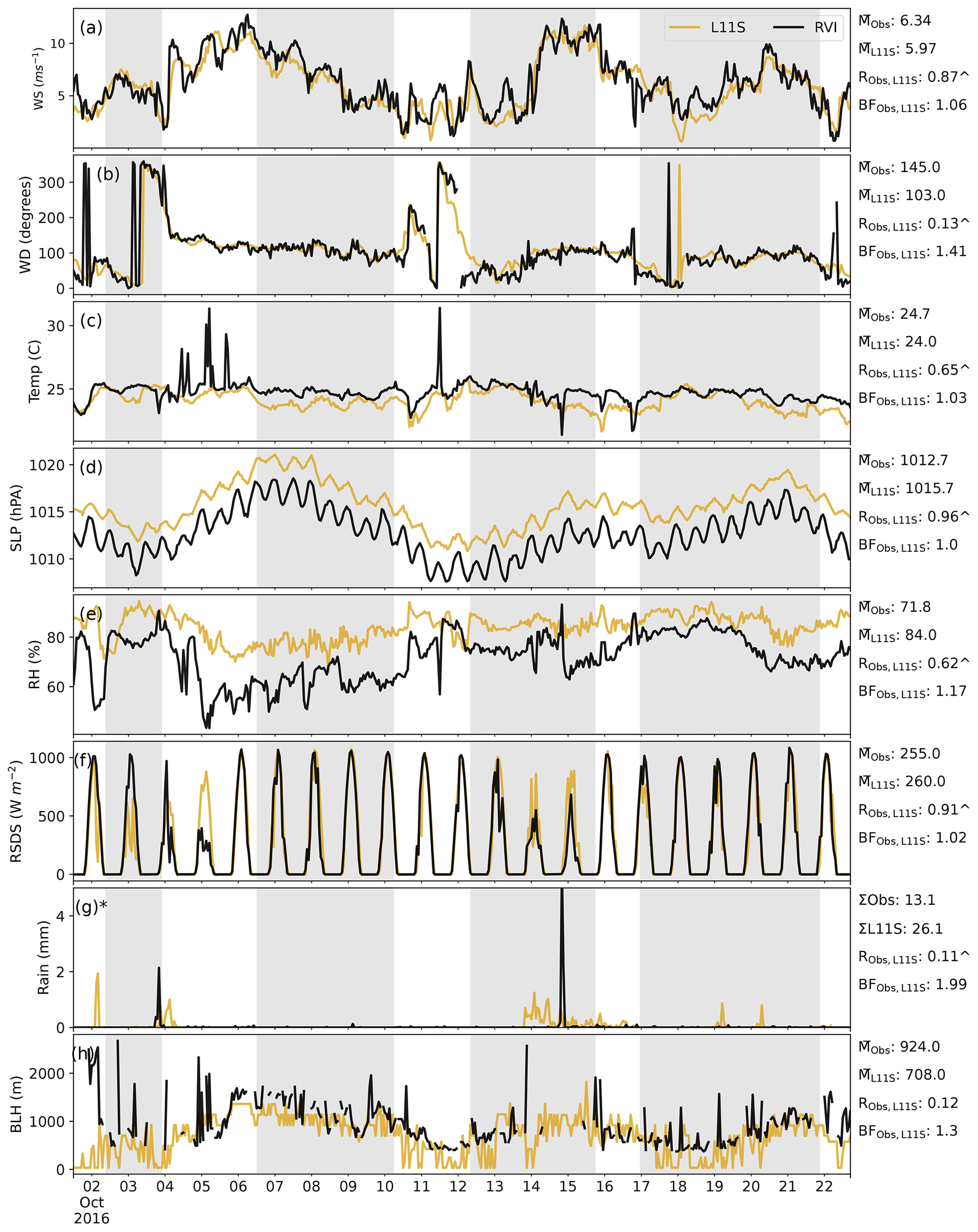
Figure C1Time series along the RVI track (in UTC) in descending order of wind speed, wind direction, temperature, sea level pressure, relative humidity, surface incoming radiation, rainfall and boundary layer height, comparing the L11S WRF simulation (yellow) to observations (black). Summary statistics are shown for the observations and L11S including the mean () (or sum Σ), the correlation (R) and the normalised mean bias factor. ∧ indicates where the R values are significant to the 95th percentile. The shaded grey areas in (a)–(h) represent periods when the ship was at a station. The y axis in (g) has been limited to 5 mm for clarity. Observations in (h) have been filtered for when cloud was detected and subsequently excluded for the relevant statistics.

Figure C2Time series for AIRBOX (in UTC) in descending order of wind speed, wind direction, temperature, sea level pressure, relative humidity, surface incoming radiation, rainfall and boundary layer height, comparing the L11S WRF simulation (yellow) to observations (black). Summary statistics are shown for the observations and L11S including the mean () (or sum Σ), the correlation (R) and the normalised mean bias factor. ∧ indicates where the R values are significant to the 95th percentile.
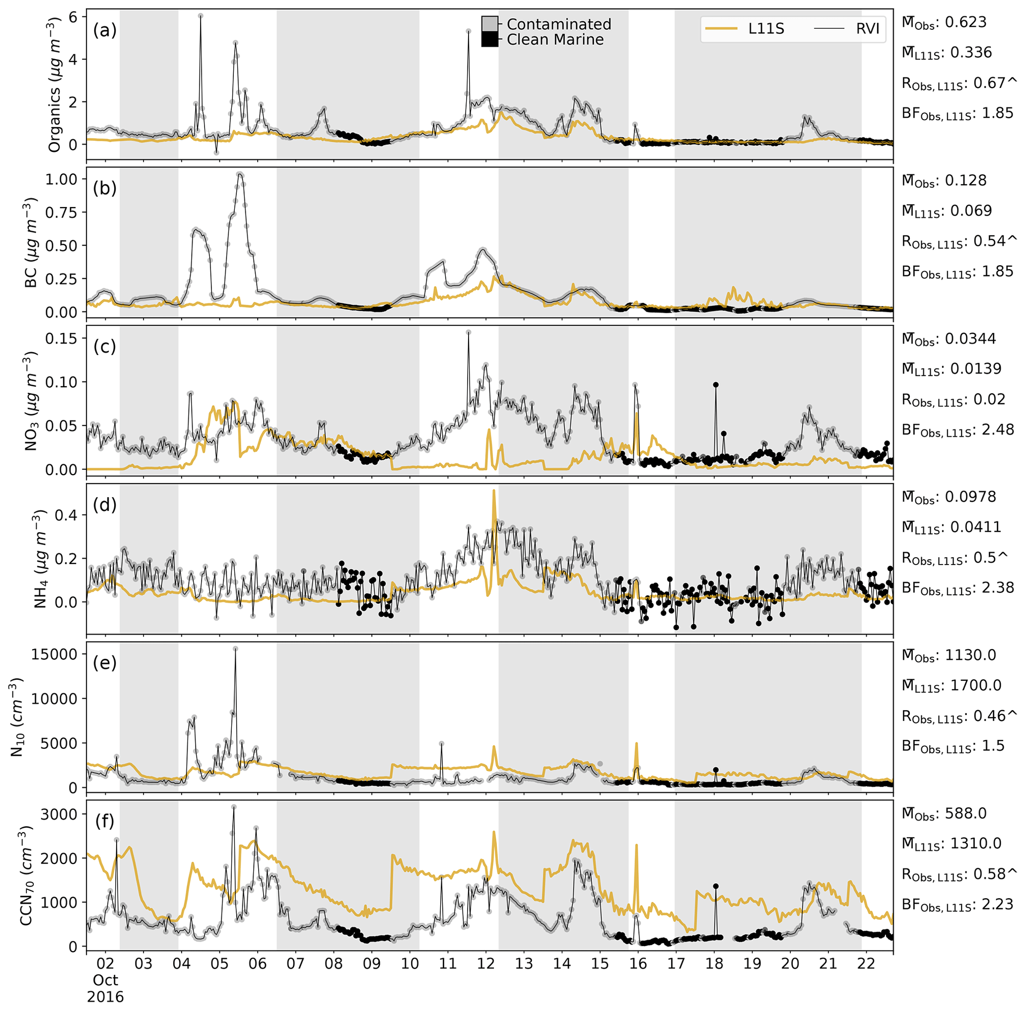
Figure C3Time series along the RVI track in descending order of surface organic, BC, NO3 and NH4 aerosol mass, aerosol number greater than 10 nm (N10) and cloud condensation nuclei greater than 70 µm (CCN70), comparing the L11S simulation (yellow) to the observations (black). Summary statistics are shown for the observations and L11S including the mean (M), the Pearson correlation (R) and the normalised mean bias factor. ∧ indicates where the R values are significant to the 95th percentile. The shaded grey areas in (a)–(f) represent periods when the ship was at a station. Observations in the time series are flagged by grey dots when the air mass was considered to be influenced by exhaust, terrestrial air mass or both (contaminated), including a log flag. Flagged values have been excluded from the statistics.

Figure C4Time series for AIRBOX in descending order of surface organic, BC, NO3 and NH4 aerosol mass and aerosol number greater than 10 nm (N10), comparing the L11S simulation (yellow) to the observations (black). Summary statistics are shown for the observations and L11S including the mean (M), the Pearson correlation (R) and the normalised mean bias factor. ∧ indicates where the R values are significant to the 95th percentile.
RVI (voyage IN2016_V05) data including ship location, meteorology and radon are available on the CSIRO Marlin Metadata System at https://marlin.csiro.au/ (CSIRO National Collections and Marine Infrastructure, 2022). Remaining RVI and AIRBOX data are available upon request. WRF-Chem namelists are available upon request, and data can be made available upon reasonable request. WRF-Chem analysis was performed using the wrf-python software package (https://doi.org/10.5065/D6W094P1, Ladwig, 2017).
SLF completed the WRF-Chem simulations, analysis and the initial draft of this paper. SU developed the initial model set-up and provided advice as to the specific set-up requirements of this study. MTW and SU helped guide the analysis and contributed significantly to the revisions of this paper. RS and TPL provided advice and guidance on the direction of this study and contributed to the revisions of this paper. Remaining authors contributed observational data to this study and to the revisions of this paper.
The contact author has declared that neither they nor their co-authors have any competing interests.
Publisher’s note: Copernicus Publications remains neutral with regard to jurisdictional claims in published maps and institutional affiliations.
This study and its authors were supported by the ARC Discovery Project: Great Barrier Reef as a significant source of climatically relevant aerosol particles (DP150101649). Sonya L. Fiddes would like to thank Peter J. Rayner and his research group for their helpful discussions, Mary Bath for her constructive comments for Sonya's PhD thesis examination and Dylan McConnell for providing the locations of power generators across Queensland. Sonya L. Fiddes was supported by the Australian Research Council (ARC) Centre of Excellence for Climate System Science (CE110001028) and the Australian Antarctic Program Partnership. Todd P. Lane is supported by the Australian Research Council (ARC) Centre of Excellence for Climate Extremes (CE170100023). Financial support was given to Hiroshi Tanimoto and Yuko Omori by Grant-in-Aid for Scientific Research (15H01732 and 17KK0016) from the Ministry of Education, Culture, Sports, Science and Technology, Japan. This research was undertaken with the assistance of resources and services from the National Computational Infrastructure (Project q90 and w40), which is supported by the Australian Government. Sonya L. Fiddes was supported by the Australian Government Research Training Program Scholarship.
This research has been supported by the Australian Research Council (grant nos. DP150101649, CE170100023, and CE110001028) and the Grant-in-Aid for Scientific Research (15H01732 and 17KK0016) from the Ministry of Education, Culture, Sports, Science and Technology, Japan.
This paper was edited by Susannah Burrows and reviewed by two anonymous referees.
Abdul-Razzak, H. and Ghan, S. J.: A parameterization of aerosol activation: 2. Multiple aerosol types, J. Geophys. Res.-Atmos., 105, 6837–6844, https://doi.org/10.1029/1999JD901161, 2000. a
Abdul-Razzak, H. and Ghan, S. J.: A parameterization of aerosol activation 3. Sectional representation, J. Geophys. Res.-Atmos., 107, 1–6, https://doi.org/10.1029/2001jd000483, 2002. a
Albrecht, B. A.: Aerosols, cloud microphysics, and fractional cloudiness, Science, 245, 1227–1230, https://doi.org/10.1126/science.245.4923.1227, 1989. a
Alexander, S. P. and Protat, A.: Cloud Properties Observed From the Surface and by Satellite at the Northern Edge of the Southern Ocean, J. Geophys. Res.-Atmos., 123, 443–456, https://doi.org/10.1002/2017JD026552, 2018. a, b
Alexander, S. P. and Protat, A.: Vertical Profiling of Aerosols With a Combined Raman‐Elastic Backscatter Lidar in the Remote Southern Ocean Marine Boundary Layer (43–66∘ S, 132–150∘ E), J. Geophys. Res.-Atmos., 124, 12107–12125, https://doi.org/10.1029/2019JD030628, 2019. a
Alexander, S. P., McFarquhar, G. M., Marchand, R., Protat, A., Vignon, E., Mace, G. G., and Klekociuk, A. R.: Mixed‐Phase Clouds and Precipitation in Southern Ocean Cyclones and Cloud Systems Observed Poleward of 64∘ S by Ship‐Based Cloud Radar and Lidar, J. Geophys. Res.-Atmos., 126, e2020JD033626, https://doi.org/10.1029/2020JD033626, 2021. a
Allan, J. D., Delia, A. E., Coe, H., Bower, K. N., Alfarra, M. R., Jimenez, J. L., Middlebrook, A. M., Drewnick, F., Onasch, T. B., Canagaratna, M. R., Jayne, J. T., and Worsnop, D. R.: A generalised method for the extraction of chemically resolved mass spectra from Aerodyne aerosol mass spectrometer data, J. Aerosol Sci., 35, 909–922, https://doi.org/10.1016/j.jaerosci.2004.02.007, 2004. a
Baars, H., Ansmann, A., Engelmann, R., and Althausen, D.: Continuous monitoring of the boundary-layer top with lidar, Atmos. Chem. Phys., 8, 7281–7296, https://doi.org/10.5194/acp-8-7281-2008, 2008. a, b
Barker, H., Pincus, R., and Morcrette, J.-J.: The Monte-Carlo Independent Column Approximation: Application within large-scale models, in: Proceedings of the GCSS/ARM Workshop on the Representation of Cloud Systems in Large-Scale Models, p. 10, May 2002, Kananaskis, Alberta, Canada, https://www.researchgate.net/publication/247932508_The_Monte_Carlo_Independent_Column_Approximation_Application_within_large-scale_models (last access: 11 February 2022), 2003. a
Bell, T. G., Landwehr, S., Miller, S. D., de Bruyn, W. J., Callaghan, A. H., Scanlon, B., Ward, B., Yang, M., and Saltzman, E. S.: Estimation of bubble-mediated air–sea gas exchange from concurrent DMS and CO2 transfer velocities at intermediate–high wind speeds, Atmos. Chem. Phys., 17, 9019–9033, https://doi.org/10.5194/acp-17-9019-2017, 2017. a
Blichner, S. M., Sporre, M. K., and Berntsen, T. K.: Reduced effective radiative forcing from cloud–aerosol interactions (ERFaci) with improved treatment of early aerosol growth in an Earth system model, Atmos. Chem. Phys., 21, 17243–17265, https://doi.org/10.5194/acp-21-17243-2021, 2021. a, b
Bohren, C. F. and Huffman, D. R.: Absorption and Scattering of Light by Small Particles, Wiley, Weinheim, Germany, https://doi.org/10.1002/9783527618156, 1998. a
Brean, J., Dall’Osto, M., Simó, R., Shi, Z., Beddows, D. C. S., and Harrison, R. M.: Open ocean and coastal new particle formation from sulfuric acid and amines around the Antarctic Peninsula, Nat. Geosci., 14, 383–388, https://doi.org/10.1038/s41561-021-00751-y, 2021. a
Breider, T. J., Chipperfield, M. P., Richards, N. A., Carslaw, K. S., Mann, G. W., and Spracklen, D. V.: Impact of BrO on dimethylsulfide in the remote marine boundary layer, Geophys. Res. Lett., 37, 1–6, https://doi.org/10.1029/2009GL040868, 2010. a
Broadbent, A., Jones, G. B., and Jones, R. J.: DMSP in Corals and Benthic Algae from the Great Barrier Reef, Estuar. Coast. Shelf S., 55, 547–555, https://doi.org/10.1006/ecss.2002.1021, 2002. a
Broadbent, A. D. and Jones, G. B.: DMS and DMSP in mucus ropes, coral mucus, surface films and sediment pore waters from coral reefs in the Great Barrier Reef, Mar. Freshwater Res., 55, 849–855, https://doi.org/10.1071/MF04114, 2004. a
Burdett, H. L., Hatton, A. D., and Kamenos, N. A.: Coralline algae as a globally significant pool of marine dimethylated sulfur, Global Biogeochem. Cy., 29, 1845–1853, https://doi.org/10.1002/2015GB005274, 2015. a
Charlson, R. J., Lovelock, J. E., Andreae, M. O., and Warren, S. G.: Oceanic phytoplankton, atmospheric sulphur, cloud albedo and climate, Nature, 326, 655–661, https://doi.org/10.1038/326655a0, 1987. a
Chen, F. and Dudhia, J.: Coupling an Advanced Land Surface–Hydrology Model with the Penn State–NCAR MM5 Modeling System. Part II: Preliminary Model Validation, Mon. Weather Rev., 129, 587–604, https://doi.org/10.1175/1520-0493(2001)129<0587:caalsh>2.0.co;2, 2002. a
Chen, G., Li, S., Knibbs, L. D., Hamm, N. A., Cao, W., Li, T., Guo, J., Ren, H., Abramson, M. J., and Guo, Y.: A machine learning method to estimate PM2.5 concentrations across China with remote sensing, meteorological and land use information, Sci. Total Environ., 636, 52–60, https://doi.org/10.1016/j.scitotenv.2018.04.251, 2018. a, b
Chen, Z., Schofield, R., Rayner, P., Zhang, T., Liu, C., Vincent, C., Fiddes, S., Ryan, R. G., Alroe, J., Ristovski, Z. D., Humphries, R. S., Keywood, M. D., Ward, J., Paton-Walsh, C., Naylor, T., and Shu, X.: Characterization of aerosols over the Great Barrier Reef: The influence of transported continental sources, Sci. Total Environ., 690, 426–437, https://doi.org/10.1016/j.scitotenv.2019.07.007, 2019. a, b, c, d
Chin, M., Rood, R. B., Lin, S.-J., Müller, J.-F., and Thompson, A. M.: Atmospheric sulfur cycle simulated in the global model GOCART: Model description and global properties, J. Geophys. Res.-Atmos., 105, 24671–24687, https://doi.org/10.1029/2000JD900384, 2000. a
Cropp, R., Gabric, A., van Tran, D., Jones, G., Swan, H., and Butler, H.: Coral reef aerosol emissions in response to irradiance stress in the Great Barrier Reef, Australia, Ambio, 47, 671–681, https://doi.org/10.1007/s13280-018-1018-y, 2018. a, b, c, d
CSIRO: RV Investigator Voyage IN2016_V05 Underway UWY Data, http://www.marlin.csiro.au/geonetwork/srv/eng/search#!65e8e881-dafe-4ca5-8f8a-f69d83596523 (last access: 11 February 2022), 2016. a, b, c
CSIRO National Collections and Marine Infrastructure: Marlin Metadata System, https://marlin.csiro.au/, last access: 11 February 2022. a
Deschaseaux, E., Jones, G. B., Miljevic, B., Ristovski, Z., and Swan, H.: Can corals form aerosol particles through volatile sulphur compound emissions?, in: Proceedings of the 12th International Coral Reef Symposium, edited by: Yellowlees, D. and Hughes, T., James Cook University, Cairns, QLD, Australia, 2012. a
Deschaseaux, E., Stoltenberg, L., Hrebien, V., Koveke, E. P., Toda, K., and Eyre, B. D.: Dimethylsulfide (DMS) fluxes from permeable coral reef carbonate sediments, Mar. Chem., 208, 1–10, https://doi.org/10.1016/j.marchem.2018.11.008, 2019. a
Draxler, R. R. and Hess, G. D.: Description of the HYSPLIT_4 modeling system, Tech. rep., National Oceanic Atmospheric Administration, Silver Spring, Maryland, USA, https://www.arl.noaa.gov/documents/reports/arl-224.pdf (last access: 11 February 2022), 1997. a
Draxler, R. R. and Hess, G. D.: An Overview of the HYSPLIT_4 Modelling System for Trajectories, Dispersion, and Deposition, Aust. Meteorol. Mag., 47, 295–308, 1998. a
Drewnick, F., Hings, S. S., DeCarlo, P., Jayne, J. T., Gonin, M., Fuhrer, K., Weimer, S., Jimenez, J. L., Demerjian, K. L., Borrmann, S., and Worsnop, D. R.: A new time-of-flight aerosol mass spectrometer (TOF-AMS) – Instrument description and first field deployment, Aerosol Sci. Tech., 39, 637–658, https://doi.org/10.1080/02786820500182040, 2005. a, b
Emmerson, K. M., Possell, M., Aspinwall, M. J., Pfautsch, S., and Tjoelker, M. G.: Temperature response measurements from eucalypts give insight into the impact of Australian isoprene emissions on air quality in 2050, Atmos. Chem. Phys., 20, 6193–6206, https://doi.org/10.5194/acp-20-6193-2020, 2020. a
Emmons, L. K., Walters, S., Hess, P. G., Lamarque, J.-F., Pfister, G. G., Fillmore, D., Granier, C., Guenther, A., Kinnison, D., Laepple, T., Orlando, J., Tie, X., Tyndall, G., Wiedinmyer, C., Baughcum, S. L., and Kloster, S.: Description and evaluation of the Model for Ozone and Related chemical Tracers, version 4 (MOZART-4), Geosci. Model Dev., 3, 43–67, https://doi.org/10.5194/gmd-3-43-2010, 2010. a
European Commission Joint Research Centre and Netherlands Environmental Assessment Agency: Emission Database for Global Atmospheric Research (EDGAR), https://edgar.jrc.ec.europa.eu/ (last access: 11 February 2022), 2012. a
Fast, J. D., Gustafson, W. I., Easter, R. C., Zaveri, R. A., Barnard, J. C., Chapman, E. G., Grell, G. A., and Peckham, S. E.: Evolution of ozone, particulates, and aerosol direct radiative forcing in the vicinity of Houston using a fully coupled meteorology-chemistry-aerosol model, J. Geophys. Res.-Atmos., 111, 1–29, https://doi.org/10.1029/2005JD006721, 2006. a, b
Fiddes, S. L., Woodhouse, M. T., Nicholls, Z., Lane, T. P., and Schofield, R.: Cloud, precipitation and radiation responses to large perturbations in global dimethyl sulfide, Atmos. Chem. Phys., 18, 10177–10198, https://doi.org/10.5194/acp-18-10177-2018, 2018. a, b, c, d, e, f
Fiddes, S. L., Woodhouse, M. T., Lane, T. P., and Schofield, R.: Coral-reef-derived dimethyl sulfide and the climatic impact of the loss of coral reefs, Atmos. Chem. Phys., 21, 5883–5903, https://doi.org/10.5194/acp-21-5883-2021, 2021. a, b, c, d, e, f, g, h, i, j
Fröhlich, R., Cubison, M. J., Slowik, J. G., Bukowiecki, N., Prévôt, A. S. H., Baltensperger, U., Schneider, J., Kimmel, J. R., Gonin, M., Rohner, U., Worsnop, D. R., and Jayne, J. T.: The ToF-ACSM: a portable aerosol chemical speciation monitor with TOFMS detection, Atmos. Meas. Tech., 6, 3225–3241, https://doi.org/10.5194/amt-6-3225-2013, 2013. a, b
Fuentes, E., Coe, H., Green, D., de Leeuw, G., and McFiggans, G.: On the impacts of phytoplankton-derived organic matter on the properties of the primary marine aerosol – Part 1: Source fluxes, Atmos. Chem. Phys., 10, 9295–9317, https://doi.org/10.5194/acp-10-9295-2010, 2010. a, b
Gong, S. L., Barrie, L. A., and Blanchet, J.-P.: Modeling sea-salt aerosols in the atmosphere: 1. Model development, J. Geophys. Res.-Atmos., 102, 3805–3818, https://doi.org/10.1029/96jd02953, 1997. a, b, c
Gordon, H., Sengupta, K., Rap, A., Duplissy, J., Frege, C., Williamson, C., Heinritzi, M., Simon, M., Yan, C., Almeida, J., Tröstl, J., Nieminen, T., Ortega, I. K., Wagner, R., Dunne, E. M., Adamov, A., Amorim, A., Bernhammer, A.-K., Bianchi, F., Breitenlechner, M., Brilke, S., Chen, X., Craven, J. S., Dias, A., Ehrhart, S., Fischer, L., Flagan, R. C., Franchin, A., Fuchs, C., Guida, R., Hakala, J., Hoyle, C. R., Jokinen, T., Junninen, H., Kangasluoma, J., Kim, J., Kirkby, J., Krapf, M., Kürten, A., Laaksonen, A., Lehtipalo, K., Makhmutov, V., Mathot, S., Molteni, U., Monks, S. A., Onnela, A., Peräkylä, O., Piel, F., Petäjä, T., Praplan, A. P., Pringle, K. J., Richards, N. A. D., Rissanen, M. P., Rondo, L., Sarnela, N., Schobesberger, S., Scott, C. E., Seinfeld, J. H., Sharma, S., Sipilä, M., Steiner, G., Stozhkov, Y., Stratmann, F., Tomé, A., Virtanen, A., Vogel, A. L., Wagner, A. C., Wagner, P. E., Weingartner, E., Wimmer, D., Winkler, P. M., Ye, P., Zhang, X., Hansel, A., Dommen, J., Donahue, N. M., Worsnop, D. R., Baltensperger, U., Kulmala, M., Curtius, J., and Carslaw, K. S.: Reduced anthropogenic aerosol radiative forcing caused by biogenic new particle formation, P. Natl. Acad. Sci. USA, 113, 12053–12058, https://doi.org/10.1073/pnas.1602360113, 2016. a
Gordon, H., Field, P. R., Abel, S. J., Dalvi, M., Grosvenor, D. P., Hill, A. A., Johnson, B. T., Miltenberger, A. K., Yoshioka, M., and Carslaw, K. S.: Large simulated radiative effects of smoke in the south-east Atlantic, Atmos. Chem. Phys., 18, 15261–15289, https://doi.org/10.5194/acp-18-15261-2018, 2018. a
Green, T. K. and Hatton, A. D.: The Claw Hypothesis: A New Perspective on the Role of Biogenic Sulphur in the Regulation of Global Climate, Oceanogr. Mar. Biol., 52, 315–336, https://doi.org/10.1201/b17143-7, 2014. a
Grell, G. A. and Dévényi, D.: A generalized approach to parameterizing convection combining ensemble and data assimilation techniques, Geophys. Res. Lett., 29, 38-1–38-4, https://doi.org/10.1029/2002gl015311, 2002. a
Guenther, A., Zimmerman, P., and Wildermuth, M.: Natural volatile organic compound emission rate estimates for U.S. woodland landscapes, Atmos. Environ., 28, 1197–1210, https://doi.org/10.1016/1352-2310(94)90297-6, 1994. a
Gustafson, W. I., Chapman, E. G., Ghan, S. J., Easter, R. C., and Fast, J. D.: Impact on modeled cloud characteristics due to simplified treatment of uniform cloud condensation nuclei during NEAQS 2004, Geophys. Res. Lett., 34, 1–5, https://doi.org/10.1029/2007GL030021, 2007. a
Hopkins, F. E., Bell, T. G., Yang, M., Suggett, D. J., and Steinke, M.: Air exposure of coral is a significant source of dimethylsulfide (DMS) to the atmosphere, Sci. Rep.-UK, 6, 36031, https://doi.org/10.1038/srep36031, 2016. a
Hu, Y., Winker, D., Vaughan, M., Lin, B., Omar, A., Trepte, C., Flittner, D., Yang, P., Nasiri, S. L., Baum, B., Holz, R., Sun, W., Liu, Z., Wang, Z., Young, S., Stamnes, K., Huang, J., and Kuehn, R.: CALIPSO/CALIOP Cloud Phase Discrimination Algorithm, J. Atmos. Ocean. Tech., 26, 2293–2309, https://doi.org/10.1175/2009JTECHA1280.1, 2009. a
Hulswar, S., Simo, R., Galí, M., Bell, T., Lana, A., Inamdar, S., Halloran, P. R., Manville, G., and Mahajan, A. S.: Third Revision of the Global Surface Seawater Dimethyl Sulfide Climatology (DMS-Rev3), Earth Syst. Sci. Data Discuss. [preprint], https://doi.org/10.5194/essd-2021-236, in review, 2021. a, b, c
Iacono, M. J., Delamere, J. S., Mlawer, E. J., Shephard, M. W., Clough, S. A., and Collins, W. D.: Radiative forcing by long-lived greenhouse gases: Calculations with the AER radiative transfer models, J. Geophys. Res.-Atmos., 113, 2–9, https://doi.org/10.1029/2008JD009944, 2008. a
Jackson, R. L., Gabric, A., and Cropp, R.: Effects of ocean warming and coral bleaching on aerosol emissions in the Great Barrier Reef, Australia, Sci. Rep.-UK, 8, 1–11, https://doi.org/10.1038/s41598-018-32470-7, 2018. a, b, c
Jackson, R. L., Gabric, A. J., Cropp, R., and Woodhouse, M. T.: Dimethylsulfide (DMS), marine biogenic aerosols and the ecophysiology of coral reefs, Biogeosciences, 17, 2181–2204, https://doi.org/10.5194/bg-17-2181-2020, 2020a. a
Jackson, R. L., Gabric, A. J., Woodhouse, M. T., Swan, H. B., Jones, G. B., Cropp, R., and Deschaseaux, E. S.: Coral Reef Emissions of Atmospheric Dimethylsulfide and the Influence on Marine Aerosols in the Southern Great Barrier Reef, Australia, J. Geophys. Res.-Atmos., 125, e2019JD031837, https://doi.org/10.1029/2019JD031837, 2020b. a, b, c, d, e
Jacobson, M. Z., Turco, R. P., Jensen, E. J., and Toon, O. B.: Modeling coagulation among particles of different composition and size, Atmos. Environ., 28, 1327–1338, https://doi.org/10.1016/1352-2310(94)90280-1, 1994. a
Janjić, Z. I.: The Step-Mountain Eta Coordinate Model: Further Developments of the Convection, Viscous Sublayer, and Turbulence Closure Schemes, Mon. Weather Rev., 122, 927–945, https://doi.org/10.1175/1520-0493(1994)122<0927:TSMECM>2.0.CO;2, 1994. a
Janjić, Z. I.: The surface layer parameterization in the NCEP Eta Model, World Meteorological Organization-Publications-WMO TD, 4–16, 1996. a
Jayne, J. T., Leard, D. C., Zhang, X., Davidovits, P., Smith, K. A., Kolb, C. E., and Worsnop, D. R.: Development of an Aerosol Mass Spectrometer for Size and Composition Analysis of Submicron Particles, Aerosol Sci. Tech., 33, 49–70, https://doi.org/10.1080/027868200410840, 2000. a
Jones, G., Curran, M., Swan, H., and Deschaseaux, E.: Dimethylsulfide and Coral Bleaching: Links to Solar Radiation, Low Level Cloud and the Regulation of Seawater Temperatures and Climate in the Great Barrier Reef, American Journal of Climate Change, 6, 328–359, https://doi.org/10.4236/ajcc.2017.62017, 2017. a, b, c
Jones, G. B.: Coral animals combat stress with sulphur, Nature, 502, 634–635, https://doi.org/10.1038/nature12698, 2013. a, b
Jones, G. B. and Trevena, A. J.: The influence of coral reefs on atmospheric dimethylsulphide over the Great Barrier Reef, Coral Sea, Gulf of Papua and Solomon and Bismarck Seas, Mar. Freshwater Res., 56, 85–93, https://doi.org/10.1071/MF04097, 2005. a
Jones, G. B., Curran, M., Broadbent, A., King, S., Fischer, E., and Jones, R. J.: Factors affecting the cycling of dimethylsulfide and dimethylsulfoniopropionate in coral reef waters of the great barrier reef, Environ. Chem., 4, 310–322, https://doi.org/10.1071/EN06065, 2007. a, b
Jung, E. and Shao, Y.: An intercomparison of four wet deposition schemes used in dust transport modeling, Global Planet. Change, 52, 248–260, https://doi.org/10.1016/j.gloplacha.2006.02.008, 2006. a
Kameyama, S., Tanimoto, H., Inomata, S., Tsunogai, U., Ooki, A., Yokouchi, Y., Takeda, S., Obata, H., and Uematsu, M.: Equilibrator inlet-proton transfer reaction-mass spectrometry (EI-PTR-MS) for sensitive, high-resolution measurement of dimethyl sulfide dissolved in seawater, Anal. Chem., 81, 9021–9026, https://doi.org/10.1021/ac901630h, 2009. a, b
Kanaya, Y., Taketani, F., Komazaki, Y., Liu, X., Kondo, Y., Sahu, L. K., Irie, H., and Takashima, H.: Comparison of black carbon mass concentrations observed by multi-angle absorption photometer (MAAP) and continuous soot-monitoring system (COSMOS) on fukue Island and in Tokyo, Japan, Aerosol Sci. Tech., 47, 1–10, https://doi.org/10.1080/02786826.2012.716551, 2013. a, b, c
Kettle, A. J. and Andreae, M.: Flux of dimethylsulfide from the oceans : A comparison of updated data sets and flux models, J. Geophys. Res., 105, 26793–26808, https://doi.org/10.1029/2000JD900252, 2000. a, b
Kettle, A. J., Amouroux, D., Andreae, T. W., Bates, T. S., Berresheim, H., Bingemer, H., Boniforti, R., Helas, G., Leck, C., Maspero, M., Matrai, P., McTaggart, A. R., Mihalopoulos, N., Nguyen, B. C., Novo, A., Putaud, J. P., Rapsomanikis, S., Roberts, G., Schebeske, G., Sharma, S., Simó, R., Staubes, R., Turner, S., and Uher, G.: A global data base of sea surface dimethyl sulfide (DMS) measurements and a simple model to predict sea surface DMS as a function of latitude, longitude, and month, Global Biogeochem. Cy., 13, 399–444, 1999. a
Khan, M. A., Gillespie, S. M., Razis, B., Xiao, P., Davies-Coleman, M. T., Percival, C. J., Derwent, R. G., Dyke, J. M., Ghosh, M. V., Lee, E. P., and Shallcross, D. E.: A modelling study of the atmospheric chemistry of DMS using the global model, STOCHEM-CRI, Atmos. Environ., 127, 69–79, https://doi.org/10.1016/j.atmosenv.2015.12.028, 2016. a, b, c
Kloster, S., Feichter, J., Maier-Reimer, E., Six, K. D., Stier, P., and Wetzel, P.: DMS cycle in the marine ocean-atmosphere system – a global model study, Biogeosciences, 3, 29–51, https://doi.org/10.5194/bg-3-29-2006, 2006. a
Korhonen, H., Carslaw, K. S., Spracklen, D. V., Mann, G. W., and Woodhouse, M. T.: Influence of oceanic dimethyl sulfide emissions on cloud condensation nuclei concentrations and seasonality over the remote Southern Hemisphere oceans: A global model study, J. Geophys. Res.-Atmos., 113, 1–16, https://doi.org/10.1029/2007JD009718, 2008. a, b
Kulmala, M., Laaksonen, A., and Pirjola, L.: Parameterizations for sulfuric acid/water nucleation rates, J. Geophys. Res., 103, 8301, https://doi.org/10.1029/97JD03718, 1998. a
Ladwig, W.: wrf-python (Version 1.3.2), UCAR/NCAR [software], Boulder, Colorado, https://doi.org/10.5065/D6W094P1, 2017. a
Lana, A., Bell, T. G., Simó, R., Vallina, S. M., Ballabrera-Poy, J., Kettle, A. J., Dachs, J., Bopp, L., Saltzman, E. S., Stefels, J., Johnson, J. E., and Liss, P. S.: An updated climatology of surface dimethlysulfide concentrations and emission fluxes in the global ocean, Global Biogeochem. Cy., 25, 1–17, https://doi.org/10.1029/2010GB003850, 2011. a, b, c, d
Leahy, S. M., Kingsford, M. J., and Steinberg, C. R.: Do Clouds Save the Great Barrier Reef? Satellite Imagery Elucidates the Cloud-SST Relationship at the Local Scale, PLoS ONE, 8, e70400, https://doi.org/10.1371/journal.pone.0070400, 2013. a
Lee, S., Gordon, H., Yu, H., Lehtipalo, K., Haley, R., Li, Y., and Zhang, R.: New Particle Formation in the Atmosphere: From Molecular Clusters to Global Climate, J. Geophys. Res.-Atmos., 124, 7098–7146, https://doi.org/10.1029/2018JD029356, 2019. a, b
Lee, Y. H., Pierce, J. R., and Adams, P. J.: Representation of nucleation mode microphysics in a global aerosol model with sectional microphysics, Geosci. Model Dev., 6, 1221–1232, https://doi.org/10.5194/gmd-6-1221-2013, 2013 a
Liss, P. S. and Merlivat, L.: Air-Sea Gas Exchange Rates: Introduction and Synthesis, in: The Role of Air-Sea Exchange in Geochemical Cycling, edited by: Buat-Ménard, P., 113–127, Springer Netherlands, Dordrecht, https://doi.org/10.1007/978-94-009-4738-2_5, 1986. a, b, c, d, e, f, g, h
Liu, P. S. K., Deng, R., Smith, K. A., Williams, L. R., Jayne, J. T., Canagaratna, M. R., Moore, K., Onasch, T. B., Worsnop, D. R., and Deshler, T.: Transmission Efficiency of an Aerodynamic Focusing Lens System: Comparison of Model Calculations and Laboratory Measurements for the Aerodyne Aerosol Mass Spectrometer, Aerosol Sci. Tech., 41, 721–733, https://doi.org/10.1080/02786820701422278, 2007. a
Longo, K. M., Freitas, S. R., Andreae, M. O., Setzer, A., Prins, E., and Artaxo, P.: The Coupled Aerosol and Tracer Transport model to the Brazilian developments on the Regional Atmospheric Modeling System (CATT-BRAMS) – Part 2: Model sensitivity to the biomass burning inventories, Atmos. Chem. Phys., 10, 5785–5795, https://doi.org/10.5194/acp-10-5785-2010, 2010. a
Mahajan, A. S., Fadnavis, S., Thomas, M. a., Pozzoli, L., Gupta, S., Royer, S.-j., Saiz-Lopez, A., and Simó, R.: Quantifying the impacts of an updated global dimethyl sulfide climatology on cloud microphysics and aerosol radiative forcing, J. Geophys. Res.-Atmos., 120, 2524–2536, https://doi.org/10.1002/2014JD022687, 2015. a
Matsui, H., Koike, M., Kondo, Y., Takegawa, N., Wiedensohler, A., Fast, J. D., and Zaveri, R. A.: Impact of new particle formation on the concentrations of aerosols and cloud condensation nuclei around Beijing, J. Geophys. Res., 116, D19208, https://doi.org/10.1029/2011JD016025, 2011. a
McCormick, R. A. and Ludwig, J. H.: Climate Modification by Atmospheric Aerosols, Science, 156, 1358–1359, https://doi.org/10.1126/science.156.3780.1358, 1967. a
Merikanto, J., Spracklen, D. V., Mann, G. W., Pickering, S. J., and Carslaw, K. S.: Impact of nucleation on global CCN, Atmos. Chem. Phys., 9, 8601–8616, https://doi.org/10.5194/acp-9-8601-2009, 2009. a
Metzger, A., Verheggen, B., Dommen, J., Duplissy, J., Prevot, A. S. H., Weingartner, E., Riipinen, I., Kulmala, M., Spracklen, D. V., Carslaw, K. S., and Baltensperger, U.: Evidence for the role of organics in aerosol particle formation under atmospheric conditions, P. Natl. Acad. Sci. USA, 107, 6646–6651, https://doi.org/10.1073/pnas.0911330107, 2010. a
Modini, R. L., Ristovski, Z. D., Johnson, G. R., He, C., Surawski, N., Morawska, L., Suni, T., and Kulmala, M.: New particle formation and growth at a remote, sub-tropical coastal location, Atmos. Chem. Phys., 9, 7607–7621, https://doi.org/10.5194/acp-9-7607-2009, 2009. a, b, c, d, e, f
Morrison, H., Thompson, G., and Tatarskii, V.: Impact of Cloud Microphysics on the Development of Trailing Stratiform Precipitation in a Simulated Squall Line: Comparison of One- and Two-Moment Schemes, Mon. Weather Rev., 137, 991–1007, https://doi.org/10.1175/2008mwr2556.1, 2008. a, b
Muñiz-Unamunzaga, M., Borge, R., Sarwar, G., Gantt, B., de la Paz, D., Cuevas, C. A., and Saiz-Lopez, A.: The influence of ocean halogen and sulfur emissions in the air quality of a coastal megacity: The case of Los Angeles, Sci. Total Environ., 610–611, 1536–1545, https://doi.org/10.1016/j.scitotenv.2017.06.098, 2018. a, b, c
Noh, Y. J., Miller, S. D., Heidinger, A. K., Mace, G. G., Protat, A., and Alexander, S. P.: Satellite-Based Detection of Daytime Supercooled Liquid-Topped Mixed-Phase Clouds Over the Southern Ocean Using the Advanced Himawari Imager, J. Geophys. Res.-Atmos., 124, 2677–2701, https://doi.org/10.1029/2018JD029524, 2019. a
O'Connor, E. J., Illingworth, A. J., and Hogan, R. J.: A Technique for Autocalibration of Cloud Lidar, J. Atmos. Ocean. Tech., 21, 777–786, https://doi.org/10.1175/1520-0426(2004)021<0777:ATFAOC>2.0.CO;2, 2004. a
O'Dowd, C. D., Aalto, P., Hmeri, K., Kulmala, M., and Hoffmann, T.: Atmospheric particles from organic vapours, Nature, 416, 497–498, https://doi.org/10.1038/416497a, 2002. a
Omori, Y., Tanimoto, H., Inomata, S., Kameyama, S., Takao, S., and Suzuki, K.: Evaluation of using unfiltered seawater for underway measurement of dimethyl sulfide in the ocean by online mass spectrometry, Limnol. Oceanogr.-Meth., 11, 549–560, https://doi.org/10.4319/lom.2013.11.549, 2013. a, b
Omori, Y., Tanimoto, H., Inomata, S., Ikeda, K., Iwata, T., Kameyama, S., Uematsu, M., Gamo, T., Ogawa, H., and Furuya, K.: Sea-to-air flux of dimethyl sulfide in the South and North Pacific Ocean as measured by proton transfer reaction-mass spectrometry coupled with the gradient flux technique, J. Geophys. Res., 122, 7216–7231, https://doi.org/10.1002/2017JD026527, 2017. a, b
Pincus, R. and Baker, M. B.: Effect of precipitation on the albedo susceptibility of clouds in the marine boundary layer, Nature, 372, 250–252, https://doi.org/10.1038/372250a0, 1994. a
Rahn, D. A. and Garreaud, R.: Marine boundary layer over the subtropical southeast Pacific during VOCALS-REx – Part 1: Mean structure and diurnal cycle, Atmos. Chem. Phys., 10, 4491–4506, https://doi.org/10.5194/acp-10-4491-2010, 2010. a
Saide, P. E., Spak, S. N., Carmichael, G. R., Mena-Carrasco, M. A., Yang, Q., Howell, S., Leon, D. C., Snider, J. R., Bandy, A. R., Collett, J. L., Benedict, K. B., de Szoeke, S. P., Hawkins, L. N., Allen, G., Crawford, I., Crosier, J., and Springston, S. R.: Evaluating WRF-Chem aerosol indirect effects in Southeast Pacific marine stratocumulus during VOCALS-REx, Atmos. Chem. Phys., 12, 3045–3064, https://doi.org/10.5194/acp-12-3045-2012, 2012. a, b, c, d
Semeniuk, K. and Dastoor, A.: Current state of aerosol nucleation parameterizations for air-quality and climate modeling, Atmos. Environ., 179, 77–106, https://doi.org/10.1016/j.atmosenv.2018.01.039, 2018. a, b, c, d
Shao, Y., Ishizuka, M., Mikami, M., and Leys, J. F.: Parameterization of size-resolved dust emission and validation with measurements, J. Geophys. Res.-Atmos., 116, 1–19, https://doi.org/10.1029/2010JD014527, 2011. a
Simmel, M. and Wurzler, S.: Condensation and activation in sectional cloud microphysical models, Atmos. Res., 80, 218–236, https://doi.org/10.1016/j.atmosres.2005.08.002, 2006. a
Simpson, D., Guenther, A., Hewitt, C. N., and Steinbrecher, R.: Biogenic emissions in Europe: 1. Estimates and uncertainties, J. Geophys. Res., 100, 22875, https://doi.org/10.1029/95JD02368, 1995. a
Su, C.-H., Eizenberg, N., Steinle, P., Jakob, D., Fox-Hughes, P., White, C. J., Rennie, S., Franklin, C., Dharssi, I., and Zhu, H.: BARRA v1.0: the Bureau of Meteorology Atmospheric high-resolution Regional Reanalysis for Australia, Geosci. Model Dev., 12, 2049–2068, https://doi.org/10.5194/gmd-12-2049-2019, 2019. a
Sullivan, R. C., Crippa, P., Matsui, H., Leung, L. R., Zhao, C., Thota, A., and Pryor, S. C.: New particle formation leads to cloud dimming, npj Climate and Atmospheric Science, 1, 9, https://doi.org/10.1038/s41612-018-0019-7, 2018. a, b
Swan, H. B., Ivey, J. P., Jones, G. B., and Eyre, B. D.: The validation and measurement uncertainty of an automated gas chromatograph for marine studies of atmospheric dimethylsulfide, Anal. Meth., 7, 3893–3902, https://doi.org/10.1039/c5ay00269a, 2015. a, b
Swan, H. B., Jones, G. B., Deschaseaux, E. S. M., and Eyre, B. D.: Coral reef origins of atmospheric dimethylsulfide at Heron Island, southern Great Barrier Reef, Australia, Biogeosciences, 14, 229–239, https://doi.org/10.5194/bg-14-229-2017, 2017. a
Thomas, M. A., Suntharalingam, P., Pozzoli, L., Rast, S., Devasthale, A., Kloster, S., Feichter, J., and Lenton, T. M.: Quantification of DMS aerosol-cloud-climate interactions using the ECHAM5-HAMMOZ model in a current climate scenario, Atmos. Chem. Phys., 10, 7425–7438, https://doi.org/10.5194/acp-10-7425-2010, 2010. a
Tie, X.: Effect of clouds on photolysis and oxidants in the troposphere, J. Geophys. Res., 108, 4642, https://doi.org/10.1029/2003jd003659, 2003. a
Trounce, H., Ristovsky, Z., Miljevic, B., Cravigan, L., Alroe, J., Osuagwa, C., Harvey, M., Bromley, T., Grey, S., Dunne, E., Humphries, R., Keywood, M., Ward, J., Lawson, S., Protat, A., Alexander, S., Schofield, R., Ryan, R., Fiddes, S., Vincent, C., Griffith, D., Murphy, C., Naylor, T., Jones, G., Omori, Y., and Tanimoto, H.: Great Barrier Reef aerosol and cloud data from the Reef to Rainforest campaign, Earth Syst. Sci. Data Discuss., in preparation, 2022. a
Twomey, S.: Pollution and the Planetary Albedo, Atmos. Environ., 8, 1251–1256, 1974. a
Vallina, S. M., Simó, R., and Gassó, S.: What controls CCN seasonality in the Southern Ocean? A statistical analysis based on satellite-derived chlorophyll and CCN and model-estimated OH radical and rainfall, Global Biogeochem. Cy., 20, 1–13, https://doi.org/10.1029/2005GB002597, 2006. a
Vlahos, P. and Monahan, E. C.: A generalized model for the air-sea transfer of dimethyl sulfide at high wind speeds, Geophys. Res. Lett., 36, L21605, https://doi.org/10.1029/2009GL040695, 2009. a
Warner, J.: A Reduction in Rainfall Associated with Smoke from Sugar-Cane Fires – An Inadvertent Weather Modification?, J. Appl. Meteorol., 7, 247–251, https://doi.org/10.1175/1520-0450(1968)007<0247:ARIRAW>2.0.CO;2, 1968. a
Wexler, A. S., Lurmann, F. W., and Seinfeld, J. H.: Modelling urban and regional aerosols – I. model development, Atmos. Environ., 28, 531–546, https://doi.org/10.1016/1352-2310(94)90129-5, 1994. a, b
Wilks, D. S.: Statistical Methods in the Atmospheric Sciences, Elsevier, 3rd Edn., https://doi.org/10.1016/B978-0-12-385022-5.00026-9, 2011. a
Williams, A. G. and Chambers, S. D.: A History of Radon Measurements at Cape Grim, Baseline History and Recollections: 40th Anniversary Special Edition, edited by: Derek, N., Krummel, P., and Cleland, S., CSIRO 2016, 131–146, https://doi.org/10.25919/1e94-dx04, 2016. a, b, c
Xiang, Y., Zhang, T., Liu, J., Lv, L., Dong, Y., and Chen, Z.: Atmosphere boundary layer height and its effect on air pollutants in Beijing during winter heavy pollution, Atmos. Res., 215, 305–316, https://doi.org/10.1016/j.atmosres.2018.09.014, 2019. a, b
Xu, K.-M. and Randall, D. A.: A Semiempirical Cloudiness Parameterization for Use in Climate Models, J. Atmos. Sci., 53, 3084–3102, https://doi.org/10.1175/1520-0469(1996)053<3084:ASCPFU>2.0.CO;2, 1996. a
Yang, Q., W. I. Gustafson Jr., Fast, J. D., Wang, H., Easter, R. C., Morrison, H., Lee, Y.-N., Chapman, E. G., Spak, S. N., and Mena-Carrasco, M. A.: Assessing regional scale predictions of aerosols, marine stratocumulus, and their interactions during VOCALS-REx using WRF-Chem, Atmos. Chem. Phys., 11, 11951–11975, https://doi.org/10.5194/acp-11-11951-2011, 2011. a, b, c
Yu, S., Eder, B., Dennis, R., Chu, S.-H., and Schwartz, S. E.: New unbiased symmetric metrics for evaluation of air quality models, Atmos. Sci. Lett., 7, 26–34, https://doi.org/10.1002/asl.125, 2006. a, b
Zaveri, R. A.: Development and Evaluation of a Comprehensive Tropospheric Chemistry Model for Regional and Global Applications Development and Evaluation of a Comprehensive Tropospheric Chemistry Model for Regional and Global Applications, PhD thesis, Virginia Polytechnic Institute and State University, https://citeseerx.ist.psu.edu/viewdoc/download?doi=10.1.1.411.363&rep=rep1&type=pdf (last access: 11 February 2022), 1997. a
Zaveri, R. A., Easter, R. C., Fast, J. D., and Peters, L. K.: Model for Simulating Aerosol Interactions and Chemistry (MOSAIC), J. Geophys. Res.-Atmos., 113, 1–29, https://doi.org/10.1029/2007JD008782, 2008. a, b, c, d
Zhao, B., Shrivastava, M., Donahue, N. M., Gordon, H., Schervish, M., Shilling, J. E., Zaveri, R. A., Wang, J., Andreae, M. O., Zhao, C., Gaudet, B., Liu, Y., Fan, J., and Fast, J. D.: High concentration of ultrafine particles in the Amazon free troposphere produced by organic new particle formation, P. Natl. Acad. Sci. USA, 117, 25344–25351, https://doi.org/10.1073/pnas.2006716117, 2020. a
- Abstract
- Introduction
- Methods
- Results
- Discussion
- Conclusions
- Appendix A: WRF-Chem Chemistry, aerosol and physics set-up
- Appendix B: Field observation methods
- Appendix C: Additional evaluation plots
- Code and data availability
- Author contributions
- Competing interests
- Disclaimer
- Acknowledgements
- Financial support
- Review statement
- References