Cloud, precipitation and radiation responses to large perturbations in global dimethyl sulfide

Natural aerosol emission represents one of the largest uncertainties in our understanding of the radiation budget. Sulfur emitted by marine organisms, as dimethyl sulfide (DMS), constitutes one-fifth of the global sulfur budget and yet the distribution, fluxes and fate of DMS remain poorly constrained. This study evaluates the Australian Community Climate and Earth System Simulator (ACCESS) United Kingdom Chemistry and Aerosol (UKCA) model in terms of cloud fraction, radiation and precipitation, and then quantifies the role of DMS in the chemistry–climate system. We find that ACCESS-UKCA has similar cloud and radiation biases to other global climate models. By removing all DMS, or alternatively significantly enhancing marine DMS, we find a top of the atmosphere radiative effect of 1.7 and −1.4 W m⁻² respectively. The largest responses to these DMS perturbations (removal/enhancement) are in stratiform cloud decks in the Southern Hemisphere's eastern ocean basins. These regions show significant differences in low cloud ($-\mathrm{9}/+$6 %), surface incoming shortwave radiation ($+\mathrm{7}/-\mathrm{5}$ W m⁻²) and large-scale rainfall ($+\mathrm{15}/-\mathrm{10}$ %). We demonstrate a precipitation suppression effect of DMS-derived aerosol in stratiform cloud deck regions due to DMS, coupled with an increase in low cloud fraction. The difference in low cloud fraction is an example of the aerosol lifetime effect. Globally, we find a sensitivity of temperature to annual DMS flux of 0.027 and 0.019 K per Tg yr⁻¹ of sulfur, respectively. Other areas of low cloud formation, such as the Southern Ocean and stratiform cloud decks in the Northern Hemisphere, have a relatively weak response to DMS perturbations. We highlight the need for greater understanding of the DMS–climate cycle within the context of uncertainties and biases of climate models as well as those of DMS–climate observations.

1 Introduction

Current understanding of the global climate is underpinned by the concept of the radiation budget, the balance of energy entering and leaving the Earth's atmosphere. Aerosols play an important role in this budget, having direct (McCormick and Ludwig, 1967) and indirect effects via cloud processes (Albrecht, 1989; Twomey, 1974). Aerosols produce a net cooling effect at the surface, with the total aerosol effective radiative forcing estimated as −0.9 W m⁻² by the most recent Intergovernmental Panel on Climate Change (IPCC) report. The aerosol radiative forcing substantially offsets the effect of well mixed greenhouse gases' effective radiative forcing of 2.8 W m⁻² (Myhre et al., 2013b). However, large uncertainty in aerosol radiative forcing remains (±0.5 W m⁻² in the 2013 IPCC report), and is in fact the largest source of uncertainty in the overall radiation budget for the current climate (Carslaw et al., 2013; Myhre et al., 2013b). Uncertainties due to aerosols affect not only the radiation budget, but also chemical and meteorological parameters such as ozone concentration and photolysis (Kushta et al., 2014), cloud formation, albedo, temperature and precipitation (Rosenfeld et al., 2014; Rotstayn et al., 2015; Seinfeld et al., 2016).

Natural aerosol sources account for the largest portion of this uncertainty, explaining up to 45 % of the variance of aerosol forcing, compared to 34 % from anthropogenic aerosol emissions (Carslaw et al., 2013). Dimethyl sulfide (DMS) produced by marine organisms makes up approximately 19 % of global sulfur emissions, producing a DMS flux (flux_DMS) of 17.6 Tg yr⁻¹ (Sheng et al., 2015), though estimates range from 9 to 35 Tg yr⁻¹ of sulfur (Belviso et al., 2004a; Elliott, 2009; Tesdal et al., 2016; Woodhouse et al., 2010). Global DMS concentrations and fluxes remain poorly constrained by observations (Royer et al., 2015; Tesdal et al., 2016), and its role in the climate system is subject to debate (Ayers and Cainey, 2007; Quinn and Bates, 2011).

Charlson, Lovelock, Andreae and Warren (CLAW) proposed a hypothesis by which marine organisms, primarily phytoplankton, regulate their environment via the increased production of dimethyl sulfonium propionate (DMSP) when stressed, for example due to warm sea surface temperatures (SSTs) (Charlson et al., 1987). DMSP is degraded via bacterial processes to DMS in the ocean (Yoch, 2002), some of which is vented into the atmosphere (Charlson et al., 1987). Once in the atmosphere DMS has a lifetime of 1–2 days (Kloster et al., 2007; Korhonen et al., 2008), and oxidises to form sulfuric acid and ultimately contributes to the aerosol burden. This additional source of aerosol can directly or indirectly influence the radiation budget and potentially cool local SSTs (although this has not been proven in the literature), hence reducing phytoplankton stress. The DMS–climate system is summarised in Fig. 1.

Current understanding of the DMS–climate system implies that no bio-regulatory feedback exists as proposed by the CLAW hypothesis (Quinn and Bates, 2011; Woodhouse et al., 2013). However, observations show that seasonal cloud condensation nuclei (CCN) variability cannot be explained without a contribution from DMS (Korhonen et al., 2008; Vallina et al., 2006), implying that DMS is important for the longer term climate. Complicating this problem is our limited understanding of the global distribution of DMS, ultimately relying on the collection of observations collated and interpolated by Lana et al. (2011), which may not capture local DMS concentrations in certain regions such as over coral reefs (Hopkins et al., 2016) and at the poles (Kim et al., 2017; Mungall et al., 2016).

A number of studies have parameterised global oceanic DMS (or DMSP) concentrations, using primary productivity, insolation, SSTs and other fields as predictors (Anderson et al., 2001; Belviso et al., 2004b; Gali et al., 2015; Simó and Dachs, 2002). However, numerous issues arise when trying to parameterise oceanic DMS, including the lack of observations as mentioned, but also that DMS production is species-dependent and predictors are not uniformly relevant across marine biota. Halloran et al. (2010) find that two older parameterisations of DMS concentration perform little better than in the Kettle and Andreae (2000) climatology. Further uncertainty in flux_DMS arises from the parameterisation of the sea–air flux mechanism. Several parameterisations of flux_DMS exist (Liss and Merlivat, 1986; Nightingale et al., 2000; Wanninkhof, 1992), resulting in a large range of annual global flux_DMS estimates, for example, 15–35 Tg yr⁻¹ of sulfur (Elliott, 2009) or 9–35 Tg yr⁻¹ of sulfur (Tesdal et al., 2016). Both these uncertainties (in climatology and flux) can have significant consequences for our understanding of climate.

The importance of DMS in large-scale climate has been highlighted by numerous global modelling studies. Mahajan et al. (2015) (using the Lana et al., 2011 DMS climatology) and Thomas et al. (2010) (using the Kettle et al., 1999 DMS climatology) found DMS to have a radiative effect of −1.79 and −2.03 W m⁻² at the top of the atmosphere (TOA) respectively. Thomas et al. (2011) doubled surface water DMS concentrations, (DMS_w), finding a TOA radiative effect of −3.42 W m⁻². These studies perturbed DMS in the climate system in order to quantify the effect on climate, and noted that the largest changes in radiation and cloud microphysics occurred in the Southern Ocean, South Pacific Ocean and South Indian Ocean.

Other modelling studies have explored the impact of anthropogenic climate change on marine DMS production, often with opposing conclusions, making it unclear whether marine DMS production would increase or decrease with warming temperatures (Bopp et al., 2004; Cameron-Smith et al., 2011; Gabric et al., 2004; Kloster et al., 2007). Six et al. (2013) found DMS emissions were reduced by 17 % by the end of the century, primarily due to decreasing ocean pH (caused by anthropogenic CO₂ emissions). The reduced flux_DMS was found to cause an additional 0.23–0.48 K of warming by the end of the century (Six et al., 2013). Reduced flux_DMS due to ocean acidification is also modelled by Schwinger et al. (2017), who found, under the Representative Concentration Pathway (RCP) 8.5 to the year 2200, that DMS production decreases by 48 %, assuming a strong sensitivity of DMS production to changes in pH. Schwinger et al. (2017) calculated a DMS temperature sensitivity of −0.041 K per Tg yr⁻¹ of sulfur.

Laboratory experiments have found that under ocean acidification, marine organisms produce significantly less DMS (Hopkins et al., 2011). However, more recently Hopkins et al. (2018) reported that polar planktonic communities show resilience to ocean acidification. The Six et al. (2013) study found an increased flux_DMS in the polar regions, while the Schwinger et al. (2017) study did not.

Grandey and Wang (2015) attempted to determine if a significant artificial increase of marine DMS production (due to, for example, ocean fertilisation) in the oceanic ecosystem could offset future warming trends. Under a scenario where flux_DMS is increased to 46.1 Tg yr⁻¹ of sulfur, Grandey and Wang (2015) found that global temperature increases due to anthropogenic climate change under RCP4.5 were partially offset, primarily due to low- and mid-level cloud feedbacks, resulting in a radiative flux perturbation of −2.0 W m⁻². Regional changes in precipitation (both increases and decreases) were also noted, up to as much as 30 %.

The direct aerosol effect can be approximately linearly related to aerosol concentration (Myhre et al., 2013a). By contrast, aerosol–cloud processes, or the secondary aerosol indirect effects, have large uncertainties, with implications for the radiation budget (Myhre et al., 2013b). Global climate models are currently unable to capture many key physical and chemical processes and interactions in the aerosol–cloud system (Rosenfeld et al., 2014). These shortcomings add further uncertainty to quantification of the DMS–climate system. Quantification of model performance is essential in providing context and perspective to any modelling experiment.

Many DMS–climate modelling studies consider DMS under future scenarios (Bopp et al., 2004; Cameron-Smith et al., 2011; Gabric et al., 2004; Grandey and Wang, 2015; Kloster et al., 2007; Schwinger et al., 2017; Six et al., 2013). However, it is clear that our understanding of DMS in the current climate is not yet fully established, considering both modelling and observational uncertainties. Studies exploring DMS changes under current climate conditions (Mahajan et al., 2015; Thomas et al., 2010; Woodhouse et al., 2010) have completed short simulations (approximately 1 year), which are too short to be indicative of a true climatological response. Furthermore, uncertainties related to DMS emission and fate in the atmosphere are not the only barriers to the DMS–climate question. Climate model uncertainties and biases must also be considered, which have not previously been provided.

The interactions between DMS-derived sulfur, its oxidation products and the atmosphere can be highly non-linear, vary regionally and have far-reaching impacts on multiple processes in the climate system (Thomas et al., 2011). Many of the studies noted above focused on one or two aspects of the DMS–climate system, commonly reporting on the flux_DMS and its radiative and temperature effects. In this study we evaluate the whole system, examining chemical, aerosol and meteorological changes, including cloud and precipitation effects.

This study has two aims, the first of which is to assess the suitability of the ACCESS (Australian Community Climate and Earth System Simulator) UKCA (United Kingdom Chemistry and Aerosol) model for examining the role of DMS in the Earth's climate in terms of low, medium and high cloud cover, outgoing TOA shortwave (SW) and longwave (LW) radiation, incoming surface SW radiation, and precipitation. Secondly, ACCESS-UKCA is used to test the large-scale sensitivity of the present-day climate to prescribed changes in DMS_w. We aim to discuss these sensitivities not only within the specific context of the DMS–climate system, as mentioned above, over a 10-year time period, but also in the broader context of the current uncertainties in the DMS–climate system and climate modelling.

Figure 1 Schematic diagram showing the ocean–atmosphere sulfur life cycle and climate-relevant processes. Acronyms are defined as follows: sea surface temperatures (SSTs), methane sulfonic acid (MSA), dimethylsulfoniopropionate (DMSP), dimethyl sulfoxide (DMSO), dimethyl sulfide (DMS), cloud condensation nuclei (CCN) and cloud droplet number (CDN).

Three simulations are performed to explore the chemical, aerosol and meteorological implications of large DMS_w perturbations. In the first experiment, a control simulation is compared to a simulation in which all DMS_w is removed from the system to determine its current contribution to the climate. In the second experiment, the control simulation is compared to a simulation in which DMS_w is significantly increased, and the results are compared to that of the work by Grandey and Wang (2015).

This paper is organised as follows: Sect. 2 outlines the methodology used in this study, Sect. 3 evaluates how well ACCESS-UKCA performs with respect to certain satellite products, Sect. 4 analyses the sensitivity of the ACCESS-UKCA climate to large perturbations in DMS and Sect. 5 provides some discussion and concluding remarks.

2 Methods

2.1 Model description and set-up

2.1.1 ACCESS-UKCA

The ACCESS-UKCA coupled climate–chemistry model is a platform from which the influences of DMS on the large-scale climate can be evaluated. The physical atmosphere in the ACCESS model is the United Kingdom Met Office's Unified Model (UM). In this case, UM version 8.4 is used, in conjunction with the UKCA chemistry model (Abraham et al., 2012), which includes the GLObal Model of Aerosol Processes (GLOMAP)-mode aerosol scheme described in Sect. 2.1.2.

Horizontal grid resolution is 1.25^∘ latitude × 1.85^∘ longitude, with 85 vertical levels, where the model top is located at 85 km. Anthropogenic emissions are prescribed pre-2000 from the Atmospheric Chemistry and Climate Model Intercomparison Project (ACCMIP) (Lamarque et al., 2010), and post-2000 from RCP6.0 (van Vuuren et al., 2011). Biomass burning emissions are from the GFED4s database (van der Werf et al., 2017). Emissions of other species required by ACCESS-UKCA, and their original sources, including biogenic emissions, chemical precursors and primary aerosol, are described in detail in Woodhouse et al. (2015). DMS emissions are calculated within UKCA, and are described in Sect. 2.1.3. Long-lived greenhouse gas concentrations (e.g. CO₂, CH₄ and N₂O) are prescribed from the Coupled Model Intercomparison Project Phase 5 (CMIP5) and RCP6.0 recommendations. Monthly mean SST and sea ice coverage are prescribed as per the Atmospheric Model Intercomparison Project (AMIP) (Taylor et al., 2015). UKCA is coupled to the ACCESS radiation scheme via O₃, CH₄, N₂O and aerosol (direct scattering and absorption). Aerosols further influence the large-scale cloud and precipitation schemes via the cloud droplet number (CDN) concentration, allowing changes in the chemical/aerosol fields to affect the meteorology.

For this study, ACCESS-UKCA is run for the years 2000–2009, with a 1-year spin-up, 1999. The simulations are nudged to ERA-Interim (Dee et al., 2011), using the horizontal wind component and potential temperature, at 6-hourly intervals in the free troposphere. The use of nudging does not allow aerosol and cloud responses to perturbed DMS to affect synoptic-scale meteorology; hence the results here represent instantaneous responses in the climate system. Nudging was deemed desirable for this study to limit computational expense, allowing single runs of 10 years. Due to nudging, responses in the simulation may be dampened, but can be attributed directly to the DMS perturbations. The complicating effect of internal variability within the modelled system is also avoided in nudged simulations.

2.1.2 GLOMAP

The GLOMAP-mode aerosol scheme uses two-moment pseudo-modal aerosol dynamics to simulate aerosol size distributions (Mann et al., 2010, 2012). GLOMAP-mode simulates particle compositions with sulfate, sea salt, elemental and organic carbon in internally mixed modes (Mann et al., 2010). Dust is treated outside of GLOMAP-mode according to the scheme detailed in Woodward (2001). Processes simulated within GLOMAP-mode include primary emissions, new particle formation, particle growth by coagulation, condensation and cloud processing and removal by dry deposition, and in-cloud and below-cloud scavenging (Mann et al., 2010). New particle formation occurs via two mechanisms in ACCESS-UKCA: free tropospheric binary homogeneous nucleation (Kulmala et al., 1998) and organic-mediated boundary layer nucleation (Metzger et al., 2010). The aerosol size distribution is represented in four soluble modes (corresponding to nucleation, Aitken, accumulation and coarse size modes) and one insoluble mode (Aitken). A full description of the scheme can be found in Mann et al. (2010), with improvements detailed in Mann et al. (2012). Bellouin et al. (2013) compare GLOMAP-mode with an older generation aerosol scheme, finding significant differences in aerosol response to perturbations between the two schemes.

2.1.3 DMS_w climatology and flux parameterisation

The number of DMS_w observations have increased dramatically over the last 3 decades (Kettle et al., 1999; Lana et al., 2011), although significant gaps, both spatially and temporally, remain. Lana et al. (2011) use observations to derive a gridded DMS_w climatology, which is used in this study and shown in Fig. 2a. The Lana et al. (2011) climatology shows that high-latitude regions have the highest DMS_w concentrations. Significant sampling biases exist within the Lana et al. (2011) data set, with approximately half of observations collected in late spring through summer, and more than two-thirds of the data collected in the Northern Hemisphere.

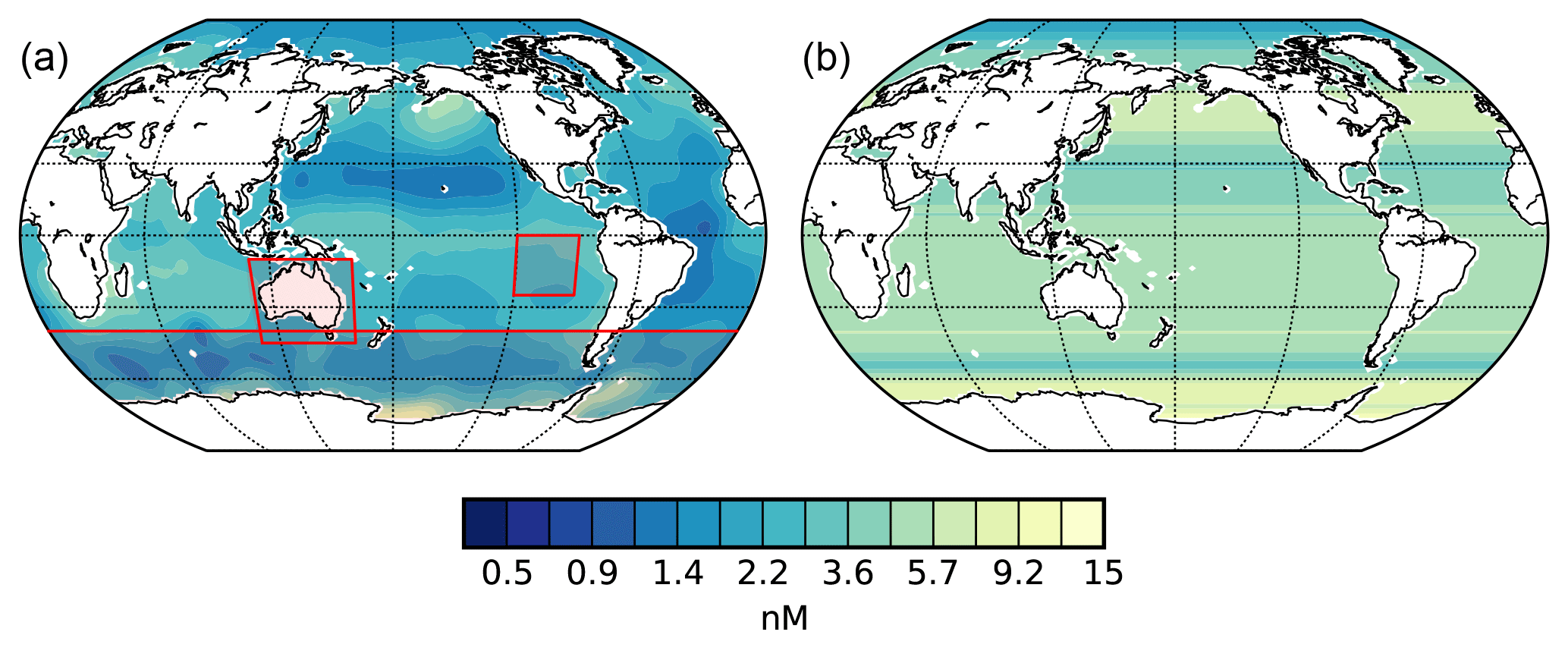
Figure 2 The annual mean concentrations of (a) the Lana et al. (2011) DMS_w climatology and (b) the DMS_w field of the second experimental run, zonal maximum DMS_w. Additionally, three regions of interest are shown in (a) by red boxes: the Australian region, 45–10^∘ S, 110–160^∘ E, the Southern Ocean (SO), ocean grid points south of 40^∘ S, and the south-eastern Pacific (SEP), 240–270^∘ E, 25^∘ S–0^∘.

The flux_DMS from the ocean to the atmosphere remains poorly parameterised, has large variability in space and time and cannot easily be measured. This subsequently causes large uncertainties in the flux_DMS parameterisation. The most common flux parameterisations exhibit considerable ranges in flux_DMS, from 15–35 Tg yr⁻¹ of sulfur in Elliott (2009) to 9–34 Tg yr⁻¹ of sulfur found in Tesdal et al. (2016), who recommend a range of 18–24 Tg yr⁻¹ of sulfur as a reasonable estimate. Vlahos and Monahan (2009) and Bell et al. (2017) show that current parameterisations overestimate the flux_DMS at high wind speeds and suggest that annual global flux_DMS is likely to be in the lower range of current estimates. Of the flux_DMS parameterisations available in ACCESS-UKCA, the Liss and Merlivat (1986) method yields a low to moderate flux comparable to those calculated in Vlahos and Monahan (2009) and Bell et al. (2017), and is used in this study.

The Liss and Merlivat (1986) DMS_flux parameterisation is described in Eq. (1), where k, the piston velocity, is parameterised under three wind-induced sea surface regimes: smooth (Eq. 2) and rough (Eq. 3) gas transfer, and a wave-breaking/bubble-bursting regime (Eq. 4).

$$\begin{array}{}\text{(1)}& {\mathrm{DMS}}_{\mathrm{flux}}=k\left({\mathrm{DMS}}_{\mathrm{w}}-{\displaystyle \frac{{\mathrm{DMS}}_{\mathrm{a}}}{\mathit{\alpha }}}\right)=k\left({\mathrm{DMS}}_{\mathrm{w}}\mathit{\alpha }-{\mathrm{DMS}}_{\mathrm{a}}\right)\end{array}$$

For w₁₀ < 3.6 m s⁻¹:

$$\begin{array}{}\text{(2)}& k=\mathrm{0.17}{w}_{\mathrm{10}}{\left({\displaystyle \frac{{\mathrm{SC}}_{\mathrm{DMS}}}{\mathrm{600}}}\right)}^{\frac{\mathrm{2}}{\mathrm{3}}}.\end{array}$$

For 3.6 m s⁻¹ < w₁₀ < 13 m s⁻¹:

$$\begin{array}{}\text{(3)}& k=\mathrm{2.85}\left(w_{\mathrm{10}}-\mathrm{3.6}\right){\left({\displaystyle \frac{{\mathrm{SC}}_{\mathrm{DMS}}}{\mathrm{600}}}\right)}^{\frac{\mathrm{1}}{\mathrm{2}}}+\mathrm{0.612}{\left({\displaystyle \frac{{\mathrm{SC}}_{\mathrm{DMS}}}{\mathrm{600}}}\right)}^{\frac{\mathrm{2}}{\mathrm{3}}}.\end{array}$$

For w₁₀ > 13 m s⁻¹:

$$\begin{array}{ll}{\displaystyle }k=& {\displaystyle }\mathrm{5.9}\left(w_{\mathrm{10}}-\mathrm{13}\right){\left({\displaystyle \frac{{\mathrm{SC}}_{\mathrm{DMS}}}{\mathrm{600}}}\right)}^{\frac{\mathrm{1}}{\mathrm{2}}}+\mathrm{26.79}\left(w_{\mathrm{10}}-\mathrm{3.6}\right){\left({\displaystyle \frac{{\mathrm{SC}}_{\mathrm{DMS}}}{\mathrm{600}}}\right)}^{\frac{\mathrm{1}}{\mathrm{2}}}\\ \text{(4)}& {\displaystyle }& {\displaystyle }+\mathrm{0.612}{\left({\displaystyle \frac{{\mathrm{SC}}_{\mathrm{DMS}}}{\mathrm{600}}}\right)}^{\frac{\mathrm{2}}{\mathrm{3}}}.\end{array}$$

Here DMS_w solubility α=11.4 at 26 ^∘C, w₁₀=10 m wind speed (m s⁻¹) and the Schmidt number of DMS SC_DMS, a measure of viscosity/diffusion and a function of sea surface temperature, is determined following the method of Saltzman et al. (1993). The denominator in this function is the Schmidt number of CO₂ in fresh water at 20 ^∘C, SC${}_{{\mathrm{CO}}_{\mathrm{2}}}=\mathrm{600}$, which is used to normalise the numerator (SC_DMS). We assume that the concentration of DMS_a is negligible, as it is orders of magnitude smaller than that of seawater.

2.2 Model evaluation

In order to provide a climatological evaluation of ACCESS-UKCA, and to put the sensitivity testing of DMS into a real-world context, a comparison to observational data sets is presented. Global means at the surface are calculated over the 2000–2009 period, except for the cloud climatologies which were only available from 2006 to 2009.

The following global data sets were compared to the model output: low, medium and high cloud fractions from the GCM-Oriented Cloud-Aerosol Lidar and Infrared Pathfinder Satellite Observation Cloud Product (CALIPSO-GOCCP) (Chepfer et al., 2010), radiation fluxes from the Clouds and the Earth's Radiant Energy System (CERES) Energy Balanced and Filled (EBAF) TOA Edition 4.0 (Loeb et al., 2009) and CERES EBAF Surface Edition 4.0 (Kato et al., 2013) and precipitation from the Tropical Rainfall Measuring Mission (TRMM) (Huffman et al., 2007). Cloud fraction is defined according to the CALIPSO-GOCCP: high between 50 and 440 hPa, medium between 440 and 680 hPa and low between 680 and 1000 hPa. Direct comparison of cloud fractions between model output and satellites cannot take into account satellite measurement biases, which can be resolved using a cloud satellite simulator such as the Cloud Feedback Model Intercomparison Program (CFMIP) Observation Simulator Package (COSP). COSP was not available in the version of ACCESS-UKCA used here, limiting the comparison. Nevertheless, a useful comparison is still possible.

2.3 DMS sensitivity testing

To explore the sensitivity of the global climate to large perturbations in DMS_w concentrations, two experimental simulations were performed and compared to the control run (Ctl). As described above, the Ctl simulation used the Lana et al. (2011) DMS_w climatology, which is shown in Fig. 2a.

In Experiment 1 (Exp.1), DMS_w was set to zero, leaving a flux of 0.72 Tg yr⁻¹ of sulfur derived from terrestrial sources (Jardine et al., 2015). From this we can attribute what role ocean-derived DMS plays in shaping our current climate and enhance our understanding of how the physical processes underpinning the DMS–climate system operate. This may further aid our understanding of how natural aerosols interact with the global radiation budget. In Experiment 2 (Exp.2), the DMS_w field was set to each latitude's (at the model resolution of 1.25^∘) monthly zonal maximum value, following a similar method to Grandey and Wang (2015), and shown in Fig. 2b. This simulation allows further exploration of the physical processes by which DMS can influence the climate, when the perturbations are exaggerated.

Three regions of interest are defined for their relevance to the broader Australian community (for which ACCESS is purposed) or are of particular interest in the DMS–climate system. They are the Australian region, 45–10^∘ S, 110–160^∘ E, the Southern Ocean (SO), ocean grid points south of 40^∘ S, and the south-eastern Pacific (SEP) that represents an area of significant stratiform cloud decks, 240–270^∘ E, 25^∘ S–0^∘.

2.4 Global energy budget

Due to the nudging of the model to ERA-Interim and the prescribed SSTs, a direct estimate of how global temperatures might respond to DMS perturbations is not possible. For this reason, a simple energy balance model has been used to estimate the effects of the DMS perturbations on global mean temperatures, a useful metric for comparison to some previous studies.

We have used the climate component of the Finite Amplitude Impulse Response (FAIR) model. This model is based on the one first proposed by Boucher and Reddy (2008) and subsequently used in the most recent IPCC Assessment Report 5 for equivalent emission metric calculations (Myhre et al., 2013b). FAIR's climate component is a simple impulse response model which emulates the behaviour of more complex Earth system models, given a certain radiative forcing (in this case due to DMS). FAIR has been designed to determine temperature responses to radiative forcing of similar magnitudes to the DMS radiative effect (Millar et al., 2017). FAIR's temperature response is calculated as the sum of two components, approximately representing the response of the upper mixed layer and deep ocean to a change in radiative forcing (Millar et al., 2017). Due to its simplicity, FAIR cannot capture the non-linearities and feedbacks in the climate system, and hence the temperature response calculated must be taken as an estimate only. Furthermore, in this work we consider only a single mid-range estimate of climate sensitivity.

For each experimental run, the radiative effect (R_DMS) due to increasing or decreasing DMS_w is defined as the difference between the TOA energy balance (Q^*) of an experimental run from the Ctl, which can be taken directly from ACCESS-UKCA. By providing this radiative effect to FAIR's climate component, we can estimate the difference in temperature expected across the 10-year period under zero DMS_w or enhanced DMS_w conditions. In ACCESS-UKCA, an ensemble experiment would be required to provide equivalent temperature difference estimates, which would be computationally expensive.

To provide a measure of model uncertainty of the change in Q^*, we have used a moving block bootstrap (Wilks, 2011). By selecting, with replacement, blocks of size 2 (as determined by the time series auto-correlation) to create 1000 alternate time series, we are able to provide the 10th and 90th percentile confidence intervals of mean change in Q^*. This is subsequently translated into an uncertainty range for the change in temperature and flux sensitivity estimates.

3 Model evaluation

This section compares selected ACCESS-UKCA fields to satellite-derived observations. In order to give context to this evaluation, the ACCESS-UKCA output is also compared to that of the CMIP5 (general circulation models, GCMs).

3.1 Cloud fraction

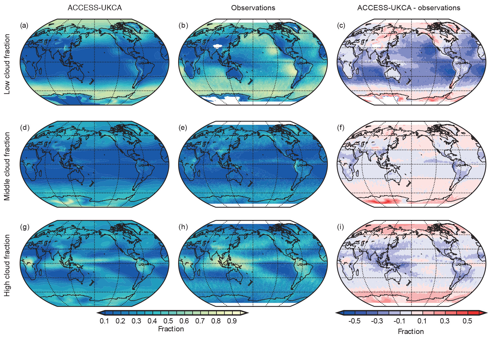
Figure 3 The 2006–2009 annual mean of the ACCESS-UKCA Ctl (a, d, g) compared to the CALIPSO-GOCCP (Chepfer et al., 2010) climatology (b, e, h), with the relative differences between the two shown in (c), (f) and (i) (model – observations). Panels (a), (b) and (c) show the low cloud fraction, (d), (e) and (f) show the middle cloud fraction and (g), (h) and (i) show the high cloud fraction.

Figure 4 As for Fig. 3 but for annual means for 2000–2009, where (a), (b) and (c) show the TOA outgoing LW radiation, (d), (e) and (f) show TOA outgoing SW radiation and (g), (h) and (i) show surface incoming SW radiation. The observations are from the CERES EBAF TOA and Surface Ed. 4.0 (Kato et al., 2013; Loeb et al., 2009); all units are in W m⁻².

The cloud fraction comparison is performed for the years 2006–2009, aligning with the availability of CALIPSO-GOCCP data. ACCESS-UKCA simulates too little low cloud fraction (Fig. 3a–c) over the majority of the globe (mean bias of −0.16), which is consistent with findings for the CMIP5 GCMs (Cesana and Chepfer, 2012; Klein et al., 2013; Nam et al., 2012). Areas of large stratiform cloud decks in eastern ocean basins are significantly underestimated, by a fraction larger than 0.5, consistent with other CMIP5 and CFMIP Phase 1 and 2 findings (Bony and Dufresne, 2005; Cesana and Chepfer, 2012; Klein et al., 2013). These low-level marine clouds have an important impact on the global radiation budget (Leon et al., 2009) and have been identified as the primary source of uncertainty in tropical cloud–climate feedbacks (e.g. the effects of the cloud albedo) in GCMs (Bony and Dufresne, 2005). These biases have been attributed to poor vertical distribution of clouds in the models, difficulty capturing overlapping cloud layers, the misrepresentation of cloud structures, deficiencies with the statistical parameterisation of clouds and likely problems in the cloud microphysics (Nam et al., 2012). Low clouds over the polar regions and some areas of northern Asia and North America are slightly overestimated. The ACCESS-UKCA low-cloud biases over the Arctic are within the range of biases found for the CMIP5 GCMs studied in Cesana and Chepfer (2012). It should be noted that satellite observations are subject to biases in detecting low clouds, particularly over the Southern Ocean.

ACCESS-UKCA reproduces medium cloud fraction (Fig. 3d–f) reasonably well, within ±0.1 in most regions (global mean bias of −0.01). The largest discrepancies are overestimated medium cloud fraction over the Southern Ocean and Antarctica, where the simulated medium cloud fraction is at its highest globally. The Antarctic bias is of opposite sign to the CMIP5 models compared in Cesana and Chepfer (2012). Bodas-Salcedo et al. (2014) note that issues within GCMs around distinguishing between clouds with tops at actual mid-level and low-level clouds contribute to such biases. The biases in high cloud fractions (Fig. 3g–i) show similar spatial patterns to that of the low cloud fraction, where an underestimate occurs over most of the tropics and mid-latitudes. The global mean bias is 0.05. The largest negative biases, of up to 0.3, occur over the Maritime Continent. Moderate overestimation is noted over the polar regions. These biases are within the range of those found for the CMIP5 models studied in Cesana and Chepfer (2012).

Interestingly, Nam et al. (2012) noted that due to underestimated low clouds in the tropics, the CMIP5 models overcompensated by producing low clouds that are optically thick and too bright and more high clouds, impacting the radiation budget. Here, an underestimation of low clouds is also found, although there is no evidence of an overcompensation of high clouds. Predominantly a small underestimation of high cloud fraction is found in this simulation at tropical to mid-latitudes (Fig. 3i).

3.2 Radiation

The remaining analyses consider means over the period of 2000–2009. The comparison of the observed and simulated TOA outgoing LW radiation is shown in Fig. 4a–c. The observed global mean of 239.7 W m⁻² is closely matched by the simulated 241.0 W m⁻². Compared to the CMIP5 ensemble, which tends to underestimate TOA outgoing LW radiation, 238.6 W m⁻² from Stephens et al. (2012) and 238.9 W m⁻² from Wang and Su (2013), TOA outgoing LW radiation in ACCESS-UKCA is slightly overestimated. The regions with the largest biases (both positive and negative) occur in regions of deep convection (Fig. 4c), and align well spatially with the biases in high cloud fractions shown in Fig. 3c. Underestimation by −3 W m⁻² of TOA outgoing LW radiation occurs over the polar oceans, which may partly be explained by an overestimation of cloud fraction at all levels, and especially the mid-level clouds (Fig. 3f) in this region.

Spatial biases in the TOA outgoing SW radiation (Fig. 4d–f) are of greater magnitude than that of the LW radiation. In most regions the sign of the outgoing SW radiation bias is opposite to that of the LW radiation. The same processes as described above that block LW radiation from escaping the atmosphere prevent SW radiation reaching the surface, hence reflecting more sunlight and enhancing the albedo. Globally, ACCESS-UKCA performs reasonably well, simulating the global mean TOA outgoing SW radiation of 101.8 W m⁻² compared to the observed 99.6 W m⁻², consistent with the multi-model mean of GCM ensembles from previous studies (Stephens et al., 2012; Wang and Su, 2013). In Fig. 4f, an abrupt change in sign of TOA outgoing SW radiation at 60^∘ S is found, which is also present in the CFMIP comparisons (Bodas-Salcedo et al., 2014). In the Southern Ocean, wrongly assigned mid-level cloud types have been found to be a leading cause of the model underestimation of TOA outgoing SW radiation (Bodas-Salcedo et al., 2014). In addition, poor representation of the physical processes surrounding supercooled liquid water in the Southern Ocean has been found to account for 27–38 % of the total reflected solar radiation (Bodas-Salcedo et al., 2016). Over the Antarctic ice sheets, both TOA outgoing and surface incoming SW radiation are overestimated, due to an underestimation of low clouds, which allows the high albedo to reflect too much incoming SW radiation back out to space.

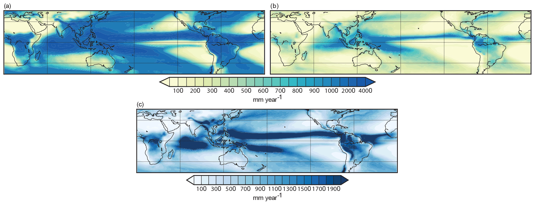
Figure 5 The mean (2000–2009) annual total precipitation of (a) the ACCESS-UKCA climatology (b) the satellite climatology from TRMM (Huffman et al., 2007) and (c) the difference between ACCESS-UKCA and the TRMM product (model – observations). Units are in mm yr⁻¹.

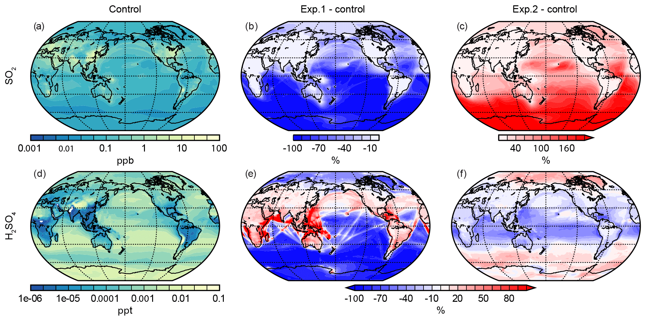
Figure 6 Mean (2000–2009) values for the Ctl (a, d), the difference between Exp.1 (zero DMS_w) and the Ctl (b, e) and the difference between Exp.2 (zonally enhanced DMS_w) and the Ctl (c, f). Panels (a), (b) and (c) show the volume mixing ratio of SO₂ in ppb; (d), (e) and (f) show the volume mixing ratio of H₂SO₄ in ppt.

Globally, ACCESS-UKCA overestimates incoming surface SW radiation (Fig. 4g–i), with 202.4 W m⁻² compared to observations of 198.3 W m⁻². This overestimation is slightly greater than that found for CMIP5 GCMs of 2 ± 6 W m⁻² (Stephens et al., 2012), though within their uncertainty. Nevertheless, large regional biases of over ±30 W m⁻² exist. The most notable features, apart from those discussed above, are too much incoming SW radiation over the continents and the tropical regions, which can be attributed in part to the underestimated cloud cover. The North Pacific and North Atlantic oceans, the Arctic Ocean and parts of the Southern Ocean all receive too little incoming SW radiation, consistent with overestimated cloud cover.

3.3 Precipitation

Precipitation in ACCESS-UKCA has large positive biases in regions that receive the most annual rainfall and align with the intertropical and South Pacific convergence zones (ITCZ/SPCZ). These regions overestimate precipitation by over 2000 mm yr⁻¹. Poor performance of GCMs in this region is not unusual however (Stephens et al., 2010), with the current CMIP5 GCM ensemble overestimating precipitation in a similar region by more than 1000 mm yr⁻¹ (Flato et al., 2013). Stephens et al. (2010) found that models in these regions produce light rain too frequently, indicating that convective processes are poorly simulated. Two of Australia's CMIP5 GCMs, ACCESS 1.0 and 1.3, both overestimate precipitation in this region by similar amounts to that of the ACCESS-UKCA model (Bi et al., 2013). If biases of precipitation are considered as a percentage (not shown), the largest differences occur in the eastern basins of the South Pacific (493 % over the SEP region) and South Atlantic oceans (275 % from 0–25^∘ S, 330–10^∘ E).

4 DMS perturbations

This section aims to quantify the role of DMS in the large-scale climate system. Two experimental simulations have been performed, described in Sect. 2.3 and Table 1, which involve removing all DMS_w (Exp.1) and setting the DMS_w to the zonal maximum (Exp.2).

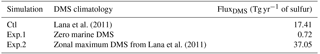
Lana et al. (2011)Lana et al. (2011)

Table 1 Summary of the three global simulations presented in this study, the DMS_w climatology used and the annual mean (2000–2009) total global flux_DMS.

4.1 Exp.1: zero DMS_w

4.1.1 Chemistry response

The 2000–2009 annual mean ocean flux_DMS from ACCESS-UKCA is 17.41 Tg yr⁻¹ of sulfur, resulting in an atmospheric DMS (DMS_a) annual mean surface concentration of 81.9 ppt. Taking all marine DMS out of the model (but retaining the terrestrial source of 0.72 Tg yr⁻¹ of sulfur) results in a 94 % reduction in DMS_a at the surface; throughout the troposphere, it results in a 98 % reduction of DMS_a.

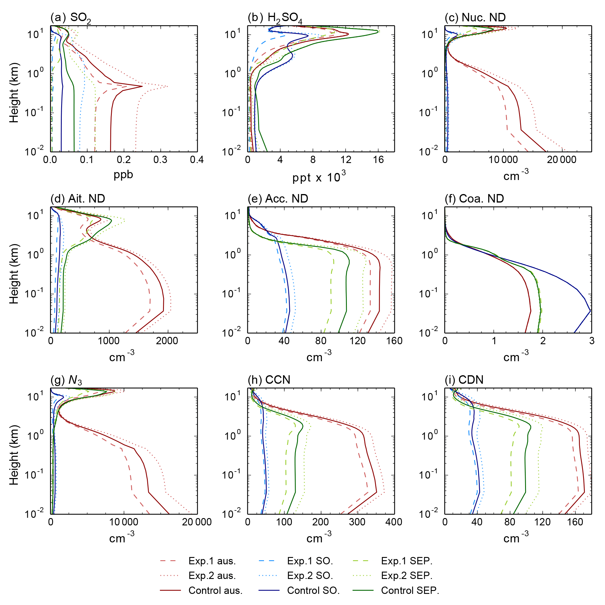
Figure 7 The vertical profiles of (a) SO₂, (b) H₂SO₄, (c) nucleation-mode number density, (d) Aitken-mode number density, (e) accumulation-mode number density, (f) coarse-mode number density, (g) N₃ nuclei number, (h) cloud condensation nuclei number and (i) cloud droplet number. The solid lines represent the Ctl, dashed lines shows Exp.1 and dotted lines show Exp.2. Blue lines show the SO (SO) mean, red the Australian (Aus) region mean and green the south-eastern Pacific (SEP). All units are cm⁻³, apart from (a) ppb and (b) ppt × 10⁻³.

The impact of this reduced flux_DMS on atmospheric sulfur can be seen in Fig. 6a–b and d–e. Globally, there is a net decrease of 15 % of SO₂ at the surface. The largest absolute differences are in the tropics and mid-latitudes over the oceans. Large relative decreases in SO₂ occur in the SO and SEP, of 84 and 94 % respectively. Figure 7a shows the vertical profile of SO₂ for the Australian region (ref), the SO (blue) and the SEP (green). The large peak in concentration at approximately 500 m occurring in the Australian profile is attributable to industrial and energy-related emissions of SO₂, which is due to lofting by chimneys and smokestacks. The SO₂ in Exp.1 is consistently lower than that of the Ctl throughout the troposphere, though for the regional means, the difference begins to decrease closer to the tropopause.

Surface H₂SO₄ (Fig. 6d–e) shows significant loss in predominantly clean marine areas; the SO has a 79 % decrease and the SEP an 84 % decrease, compared to a 49 % global mean decrease. Interestingly, heavily polluted regions, especially busy shipping lanes, undergo an increase in H₂SO₄. H₂SO₄ is a precursor gas, which can participate in the formation of secondary sulfate aerosol, or it can condense onto pre-existing particles. The increased H₂SO₄ concentration in heavily polluted regions results from a decreased condensational sink (not shown). Similar non-linearities have been described in Thomas et al. (2011).

The vertical profiles of H₂SO₄ in Fig. 7b show that the largest differences between Exp.1 and the Ctl occur in the free troposphere (between 1 and 10 km) for all regions. In all three regions (each considered a clean atmospheric environment), net decreases of H₂SO₄ occur.

4.1.2 Aerosol response

The majority of gaseous H₂SO₄ is taken up by aerosol formation (99.99 %) as opposed to being removed by dry deposition (0.01 %) (Mann et al., 2010). The peak in nucleation-mode number density in the free troposphere in Fig. 7c coincides with the peak concentration of H₂SO₄. Surface global nucleation-mode number concentration decreases by 9 % between Exp.1 and the Ctl (see Fig. 7c). While in absolute terms, clean terrestrial regions have the largest decreases, the Australian region only has a relative decrease of 18 % in nucleation-mode particles. Over the oceans, although few nucleation-mode particles exist, there are large relative differences of both signs.

In absolute terms, the differences in the aerosol number concentration are greatest in the smaller aerosol modes, particularly the nucleation mode described above. Figure 7d–f show the number concentrations for the Aitken mode, accumulation mode and coarse mode (global maps not shown). The Aitken mode (Fig. 7d) shows some differences between the two simulations, with profiles reflecting reduced new particle formation in the free troposphere and reduced condensation growth of H₂SO₄ onto pre-existing particles in the boundary layer. The largest differences are seen over the Australian region. Similar boundary layer differences are also present in the accumulation mode, with the differences between Exp.1 and the Ctl consistent below 1 km (Fig. 7e). Little difference is seen in the coarse mode throughout the troposphere (Fig. 7f), which in marine regions is dominated by sea salt.

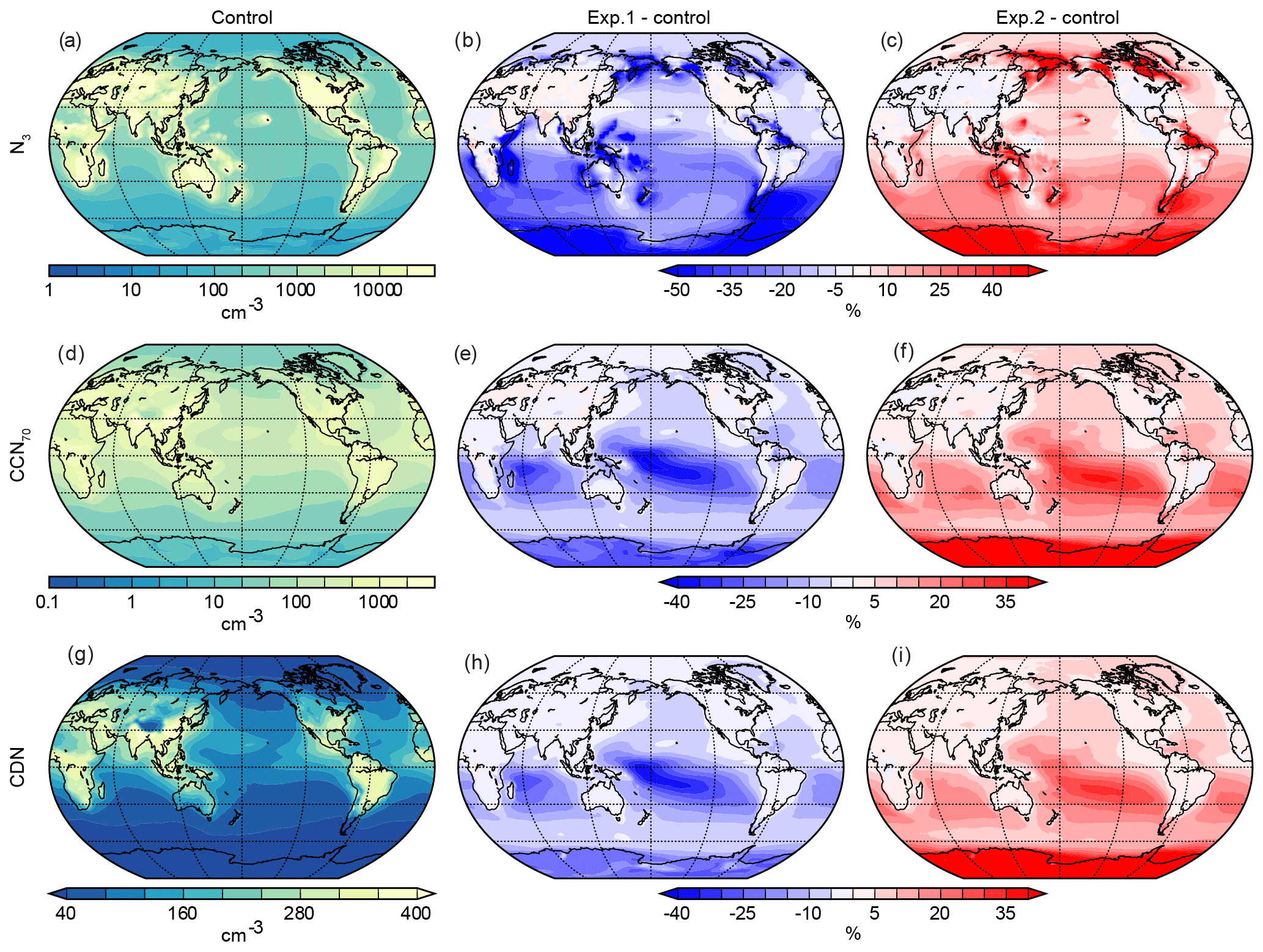
Figure 8 As for Fig. 6, but where (a), (b) and (c) the number concentration of N₃ (condensation nuclei), (d), (e) and (f) show the number of cloud condensation nuclei greater than 70 nm dry diameter and (g), (h) and (i) show the cloud droplet number concentration. All units are in cm⁻³.

As aerosols grow towards the larger end of the Aitken mode, they become relevant to cloud processes. Figure 8a shows the Ctl's N₃ (condensation) number concentration (N₃ signifies particles with a dry diameter greater than 3 nm). The difference in surface N₃ number concentration between the Ctl and Exp.1 shows the largest relative decreases occur in clean, coastal regions, predominantly in the Southern Hemisphere, as well as some regions of the SO. In heavily polluted terrestrial regions a small increase in the N₃ number concentration occurs. A decrease of 8 % is found globally. For the Australian region (representative of a clean, terrestrial region), a decrease of 17 % is found.

Over the SO a relative decrease of 39 % occurs at the surface. The SO and the SEP have far fewer aerosols in all modes except the coarse mode (see Fig. 7c–f), where sea salt dominates. This decrease in number concentration in small aerosol modes represents a large portion of the aerosol loading in the region. The increase in nucleation-mode particles is reflected in the N₃ for the SEP region, via a more moderate decrease of 20 %.

Table 2 Global and hemispheric means of the CCN sensitivity to the flux_DMS (as defined by Woodhouse et al., 2010, 2013) in both absolute (cm⁻³/$\mathrm{mg}{\mathrm{m}}^{-\mathrm{2}}{\mathrm{day}}^{-\mathrm{1}}$) and relative terms, for Exp.1 and Exp.2.

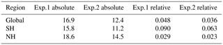
Figure 8d–e show the number concentration of CCN with dry diameters greater than 70 nm (CCN₇₀) for the Ctl and the differences resulting from Exp.1. The largest absolute differences are in the tropics, which, similarly to the N₃, have the highest concentration. Relatively, there is a global decrease of 5 %, while decreases of 7 % were found over the Australian region, decreases of 8 % over the SO and decreases of 20 % over the SEP. Differences in CDN are shown in Fig. 8g–h. The relative differences in CDN show a similar spatial pattern to that of the CCN. Global mean CDN decreases by 5 %. A decrease of 5 % is also found for the Australian region, whereas the SO shows an 8 % decrease, and the SEP shows an 18 % decrease. In both the CCN₇₀ and CDN, the marine Southern Hemisphere mid-latitudes have the largest decreases of 14 % (averaged between 5 and 35^∘ S) despite the SO having some of the larger decreases in SO₂ and H₂SO₄.

The larger differences in concentration of both CCN and CDN in the oceanic Southern Hemisphere tropics and mid-latitudes, compared to the SO, warrant further investigation of how sulfate aerosols are interacting with their background environments, for example cloud processes and pre-existing aerosols. The SO has large concentrations of sea salt particles, which, like more polluted regions of the Northern Hemisphere, may provide a buffering effect to reduced DMS-derived aerosols. Additionally, in areas of persistent low cloud formation, in-cloud aqueous sulfate oxidation is the dominant reaction (over gaseous nucleation), which allows almost instantaneous condensational growth of existing aerosols, and is temperature-dependent. We speculate that poor representation of low clouds in the SO may be having further impacts on atmospheric composition modelling than currently realised. A cloud resolving modelling study may be better suited to gain understanding of the complex system described here.

Following the method of Woodhouse et al. (2010, 2013), global and hemispheric sensitivities of CCN to flux_DMS have been calculated (Table 2). The results presented here suggest a lower CCN sensitivity to flux_DMS compared to the Woodhouse et al. (2013) study where absolute sensitivities of 94 and 63 cm⁻³/$\mathrm{mg}{\mathrm{m}}^{-\mathrm{2}}{\mathrm{day}}^{-\mathrm{1}}$ of sulfur were found globally for June and December respectively. Similar CCN sensitivities are reported in the Woodhouse et al. (2010) study (63 cm⁻³/$\mathrm{mg}{\mathrm{m}}^{-\mathrm{2}}{\mathrm{day}}^{-\mathrm{1}}$ global average). The lower sensitivities in our study are likely the result of the large (near 100 %) changes in flux_DMS (the denominator). Relative CCN sensitivities calculated here compare well with the Woodhouse et al. (2010, 2013) studies. For example Woodhouse et al. (2010) finds mean hemispheric relative CCN sensitivities of 0.02 for the Northern Hemisphere and 0.07 for the Southern Hemisphere. These results highlight the greater relative importance of DMS in the Southern Hemisphere.

4.1.3 Cloud, radiation and precipitation response

Meteorological responses to the DMS perturbations must be considered carefully. As detailed in the methods section, the ACCESS-UKCA simulations are nudged to ERA-Interim potential temperature and horizontal winds, preserving synoptic-scale meteorology and limiting any feedbacks. While performing a non-nudged simulation would allow the meteorology to respond to changes in the chemistry and aerosol more freely, it would make comparison of the aerosol and meteorological responses more difficult. Within ACCESS-UKCA, GLOMAP-mode is directly coupled to the large-scale cloud and precipitation schemes via the CDN (Abraham et al., 2012), as well as the radiation scheme via aerosols and some gases (see Sect. 2.1.1). Convective rainfall and cloud formation are not directly coupled to the aerosol scheme, but can be indirectly influenced via changes in radiation (which can act on temperature and moisture, etc.).

Figure 9 Comparisons of the low cloud fraction (as a percentage) (a–b) and incoming SW radiation at surface (W m⁻²) (c–d) over the 2000–2009 period for Exp.1 (first column) and Exp.2 (second column) minus the Ctl. The absolute values for the Ctl of these fields can be seen in Figs. 3 and 4.

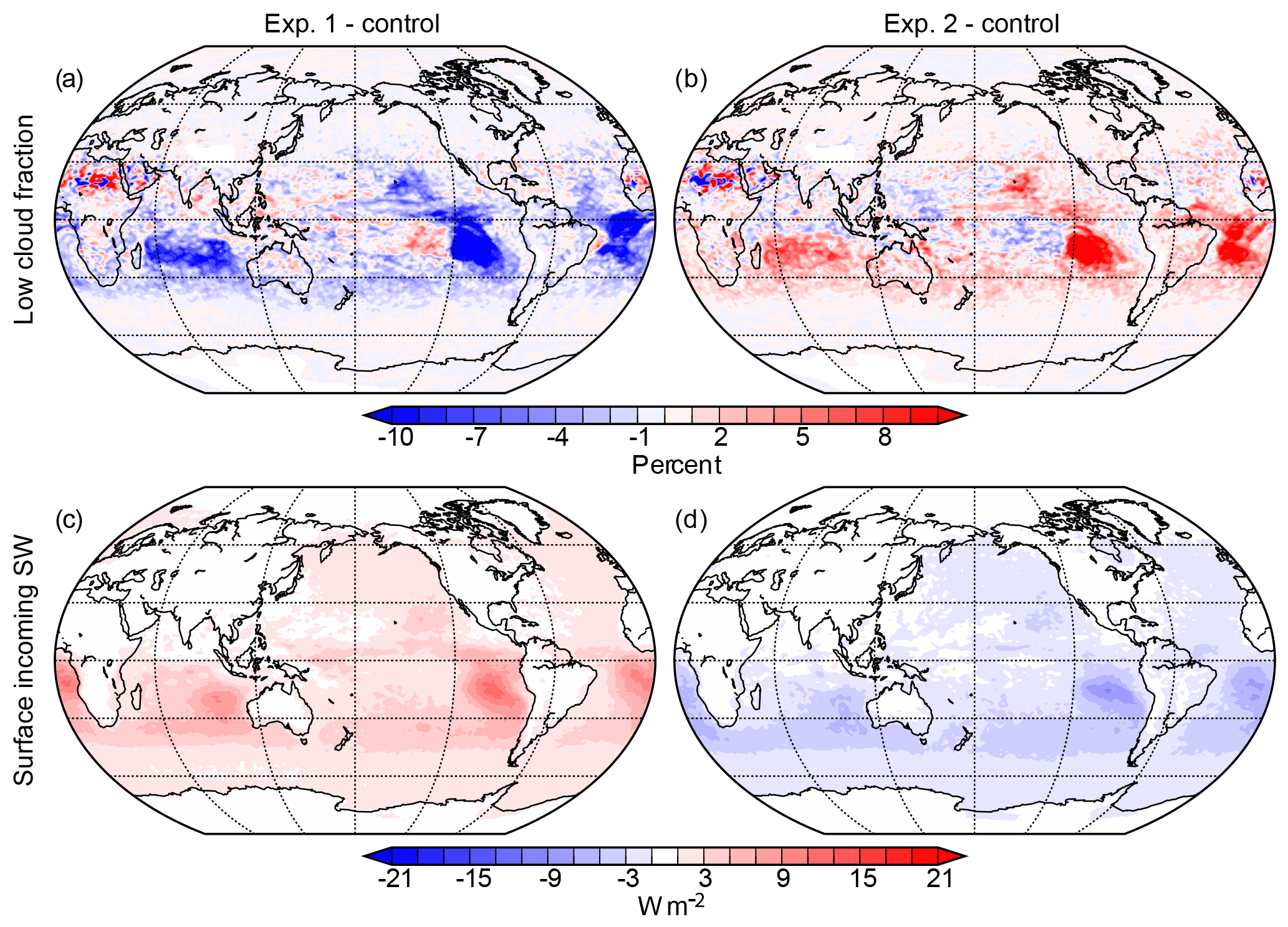
Differences in low cloud fraction occur predominantly in areas with large stratiform cloud decks (Fig. 9a). The largest differences occur in eastern basins of the Southern Hemisphere's oceans. The SEP region shows an annual mean decrease in low cloud fraction of 9 %. In the Northern Hemisphere (including the north-eastern Pacific where significant stratiform cloud decks are found) and the SO (where persistent low cloud formation occurs) only small differences are evident, which may in part be due to the modest differences in CCN and CDN concentrations discussed in Sect. 4.1.2. Stratiform cloud deck fractions are consistently underestimated by ACCESS-UKCA and other GCMs (see Sect. 3) in comparison to other areas of significant low cloud formation such as the SO. The mechanism behind the different responses (between the SO and cloud deck regions), and whether the long-standing model biases, especially those around the formation of supercooled liquid water, have contributed to the differing responses requires further investigation.

The decrease in low cloud fraction and aerosol number concentration discussed above leads to an increase in surface incoming SW radiation (Fig. 9c). This increase in surface SW radiation is highest in the regions of stratiform cloud deck formation. In the SEP region there is a mean increase of 7 W m⁻².

Figure 10 Comparisons of the (a–c) total liquid water at 1700 m height (Q_cl), (d–f) large-scale rainfall and (g–i) convective rainfall over the 2000–2009 period. The Ctl absolute values are shown in the first column, and respectively Exp.1 and Exp.2 minus the Ctl in the second and third columns. Units are in kg kg⁻¹ and mm yr⁻¹.

Decreases of total liquid water (Q_cl) at 1700 m height shown in Fig. 10a–b are found in the stratiform cloud deck regions. Little difference in Q_cl occurs at the surface. The decrease in Q_cl is coincident with increases in large-scale precipitation in the stratiform cloud decks, regions with very little precipitation (Fig. 10d–e). In the SEP region large-scale rainfall increases by 17 mm yr⁻¹ (15 %) over the Ctl mean of 111 mm yr⁻¹.

In the Southern Hemisphere stratiform cloud decks, and in particular the SEP region, the model demonstrates a distinct cloud lifetime effect in response to removing DMS in Exp.1. Decreased CDN concentration and the associated increase in cloud droplet size and increased liquid water lead to increased autoconversion and large-scale rainfall. The overall impact is to reduce low cloud fraction.

Figure 10g–h show the differences in convective rainfall. While the convective rainfall scheme is not coupled directly to GLOMAP-mode, there are differences between the simulations. Convective rainfall decreases in Exp.1 compared to the Ctl along the ITCZ (a mean difference of 11 mm yr⁻¹ between 20^∘ S and 20^∘ N). This difference represents a small fraction (less than 1 %) of the total convective rainfall. Relatively, (not shown) the largest differences (a 5 % decrease in the SEP) are found once again in eastern basins of Southern Hemisphere stratiform cloud decks.

Seifert and Beheng (2006) note that even when convection schemes are coupled to an aerosol scheme, the effects of CCN on convection, and the resultant precipitation and associated maximum updrafts, differ significantly depending on the cell type and size, making these effects difficult to quantify. Large differences in convective rainfall would not be expected in these results, due to the meteorological nudging used in the experiments.

4.2 Exp.2: zonally increased DMS_w

This section considers the response to zonally enhanced DMS_w, resulting in a flux_DMS of 37.05 Tg yr⁻¹ of sulfur (relative to 17.41 Tg yr⁻¹ of sulfur in the Ctl simulation). For comparison the Grandey and Wang (2015) study used a zonally enhanced flux_DMS of 46.1 Tg yr⁻¹ of sulfur (up from 18.2 Tg yr⁻¹ of sulfur) under global warming scenarios. Many of the differences resulting from zonally enhancing DMS_w show similar spatial patterns, with a similar magnitude but reversed sign compared to Exp.1.

Globally, the differences in SO₂ (Fig. 6c) are of comparable magnitude to Exp.1. Increased SO₂ concentrations occur over the Australian region, the SO and the SEP: increases of 42, 172 and 89 % respectively. There is a net decrease in H₂SO₄ of 14 % in Australia, and a larger decrease over the tropical oceans. Over the SO there is an increase of 9 %, while in the SEP a decrease of 37 % occurs. Similar non-linearities are discussed in terms of doubled DMS in the Thomas et al. (2011) study. These differences in SO₂ and H₂SO₄ are also clear in the vertical profiles shown in Fig. 7a–b.

Differences in the aerosol modes (see Fig. 7c–f) are of a similar magnitude but opposite sign to those noted in Sect. 4.1.2. Global mean N₃, CCN₇₀ and CDN increase by 6, 4 and 5 % respectively (Fig. 8c, f, i). Larger differences are seen over the SO of 27, 15 and 13 % and the SEP of 14, 19 and 17 % for N₃, CCN₇₀ and CDN respectively.

Globally, there is little difference in low cloud fraction or Q_cl, though increases are noted in regions of large stratiform cloud decks (Fig. 9d), which show similar spatial patterns to that of Exp.1. Incoming surface SW radiation has a global mean decrease of −1.75 W m⁻². This decrease is comparable to the Grandey and Wang (2015) finding of −2.2 W m⁻² (noting the larger DMS perturbation by Grandey and Wang, 2015). Lastly, decreases in large-scale precipitation are found, again in regions of stratiform cloud decks (Fig. 10f), while general increases in convective precipitation over the tropical oceans occur (Fig. 10i). The Grandey and Wang (2015) study, which analysed a warming climate, also found large relative decreases in precipitation rate predominantly in eastern ocean basins. We find, under the current climate, the largest relative increase in total precipitation (not shown) in the southeast basins of the Pacific and Atlantic oceans; however these results presented here are much nosier than the Grandey and Wang (2015) results. Grandey and Wang (2015) find that artificial enhancement of DMS may offset global warming, which is supported by this study as implied by the decreases in incoming SW radiation at the surface; however the precipitation responses warrant further study.

4.3 Temperature response

Table 3 Summary of the global mean (2000–2009) radiation fields: absolute Ctl values for the TOA shortwave (SW) and longwave (LW) outgoing and Q^* and the differences in these quantities resulting from Exp.1 and Exp.2 (from the Ctl) as well as the FAIR temperature response. The ranges shown for Exp.1 Ctl and Exp.2 Ctl indicate the 10th and 90th percentile confidence intervals. n/a – not applicable

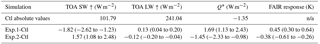
The global 2000–2009 mean of the TOA radiation budget (Q^*) and its main components are provided in Table 3, along with the relevant confidence intervals derived from the bootstrapping technique. Due to the nudging used in the simulations, we do not expect the TOA Q^* to be balanced (i.e. $Q^{*}=\mathrm{0}$). The differences in Q^* seen in Exp.1 and Exp.2, 1.69 W m⁻² (1.13 to 2.43, 10th and 90th confidence intervals) and −1.48 W m⁻² (−2.33 to −0.98, 10th and 90th confidence intervals) respectively, show a substantial radiative effect of DMS on the energy budget. The Q^* response found for Exp.1 is consistent with the Mahajan et al. (2015) findings of 1.79 W m⁻². Using the FAIR model's climate component, the 2000–2009 mean temperature response is calculated to be 0.45 K (0.30 to 0.64, 10th and 90th percentile range) for Exp.1 and −0.38 K (−0.26 to −0.61, 10th and 90th percentile range) for Exp.2.

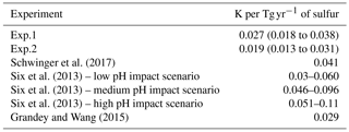
Other studies generally consider DMS changes under global warming and we can make comparisons via the sensitivity of the estimated global temperature response to changes in the flux_DMS (see Table 4). In this study, we find a response of 0.027 K per Tg yr⁻¹ of sulfur in Exp.1, and 0.019 K per Tg yr⁻¹ of sulfur in Exp.2. These results are of similar magnitude to the Grandey and Wang (2015) study (0.029 K per Tg yr⁻¹ of sulfur) and in the range of the lowest impact scenario of Six et al. (2013) (0.03–0.060 K per Tg yr⁻¹ of sulfur). The other scenarios in the Six et al. (2013) study (0.046–0.11 K per Tg yr⁻¹ of sulfur) suggest much higher temperature sensitivities to changes in flux_DMS, as does the Schwinger et al. (2017) study (0.041 K per Tg yr⁻¹ of sulfur).

Schwinger et al. (2017)Six et al. (2013)Six et al. (2013)Six et al. (2013)Grandey and Wang (2015)

Table 4 The estimated temperature response to perturbations in the flux_DMS (K per Tg yr⁻¹ of sulfur) for the current study's experiments (Exp.1 and Exp.2) and those found in the literature. The ranges shown for Exp.1 and Exp.2 indicate the 10th and 90th percentile confidence intervals.

5 Discussion and conclusions

The ACCESS-UKCA chemistry–climate model, which includes a detailed microphysical aerosol module, has been evaluated against satellite observations of cloud fraction, radiation and precipitation and subsequently used to conduct sensitivity experiments to determine the role of DMS in several aspects of the climate system.

Important considerations when using climate models include the inherent uncertainties associated with all climate simulations, e.g. emissions uncertainties (both natural and anthropogenic), parameterisations and physical representations of atmospheric processes. Nevertheless, where clear shortcomings have been found in comparison to the satellite-derived observations, the ACCESS-UKCA model has been found to perform with comparable skill to current CMIP5 GCMs. Additionally, it is important to note biases in the satellite products themselves, for example in cloud fraction retrievals as noted in Mace and Zhang (2014) or Protat et al. (2014).

Of particular interest, our evaluation of ACCESS-UKCA shows an underestimation of large stratiform cloud decks located in the eastern mid-latitude basins of the Earth's oceans. These regions of extensive low cloud produce little rainfall (that is overestimated by the model) and are often regions of high primary productivity. These biases have not been attributed to a single cause (multiple theories have been proposed, as discussed in Sect. 3.1), indicating a gap in understanding of atmospheric processes in these regions (Nam et al., 2012).

Globally, removing or enhancing DMS_w from the climate system leads to significant responses in chemistry and aerosol concentrations. While changes in meteorological parameters (low cloud fraction, large-scale precipitation, moisture, radiation) are largest in the Southern Hemisphere stratiform cloud decks, global mean differences were small. We find that DMS in these stratiform regions plays an important role in cloud processes and precipitation suppression (as discussed in Thomas et al., 2011 or with regards to anthropogenic pollution in Ackerman et al., 2004). Furthermore, we have demonstrated that marine DMS is responsible for increasing low cloud fraction in stratiform cloud deck regions, a demonstration of the second aerosol indirect (or lifetime) effect (Albrecht, 1989). These results indicate that a greater understanding of natural aerosols and their interaction with cloud processes (both via observations and modelling studies) in these regions may improve model representation, as it is these regions that show considerable model bias in comparison to observations.

In other regions of significant low cloud formation (SO, Northern Hemisphere cloud decks), aerosol sources such as sea salt and anthropogenic aerosols may buffer the regions from changes in DMS-derived aerosols. Additionally, in the SO, representation of cloud processes in global climate models is poor, especially with respect to supercooled liquid water (Bodas-Salcedo et al., 2016). It is likely that these biases are misrepresenting the DMS–climate interactions in these regions.

By nudging these simulations, the model response to the DMS perturbations is limited to fast (aerosol and cloud) changes. We suggest that free-running ensemble experiments are performed to gain insight into the aerosol–cloud–climate processes occurring in regions of significant DMS influence. Such experiments should focus on improving microphysical aspects of aerosol–cloud interaction in these regions (and how it differs among regions) or improving the representation of aerosols, in particular natural aerosols.

Previous studies examining the role of DMS in the climate system have not identified stratiform cloud decks as regions of particular importance. Instead, these studies focused on cloud feedbacks in the SO (Mahajan et al., 2015; Thomas et al., 2010). Mahajan et al. (2015) estimated the global TOA radiative effect of DMS to be 1.79 W m⁻², which is consistent with our results (1.69 W m⁻²), but slightly lower than the estimation of 2.03 W m⁻² estimated by Thomas et al. (2010) (who used the previous Kettle and Andreae (2000) DMS_w climatology).

In this study, we find the estimated temperature responses per unit change in DMS-derived sulfur flux (0.027 or 0.019 K per Tg yr⁻¹ of sulfur) are lower than those reported in the Six et al. (2013) (0.046–0.096 K per Tg yr⁻¹ of sulfur, medium-impact scenario) and Schwinger et al. (2017) (0.041 K per Tg yr⁻¹ of sulfur) studies. The temperature response sensitivities calculated here are comparable to those given in Grandey and Wang (2015) (0.029 K per Tg yr⁻¹ of sulfur). Without further information, it is difficult to speculate on the cause of the discrepancy between the results presented here and those in Six et al. (2013) and Schwinger et al. (2017). However, the discrepancy between these results suggests the need for better observational constraints, and highlights the complexity of the DMS–aerosol–cloud system.

Natural aerosols account for a significant source of uncertainty in climate modelling and radiation budgets (Carslaw et al., 2013). Our study uses the Lana et al. (2011) DMS_w climatology with the Liss and Merlivat (1986) flux parameterisation. Though this data set and method are commonplace for DMS–climate studies, both are limited by sparse observations and uncertainties (Tesdal et al., 2016). For example, recent studies have indicated that coral reefs produce significant amounts of DMS, and are an unaccounted for source of sulfur (Hopkins et al., 2016; Jones et al., 2017; Swan et al., 2017). Furthermore, larger concentrations and/or fluxes of DMS than what we currently consider have also been found at the poles, especially around sea ice and polynyas (Jarnikova and Tortell, 2016; Kim et al., 2017; Mungall et al., 2016; Nomura et al., 2011).

Observational deficiencies become particularly relevant when considering the stratiform cloud deck regions. In the Lana et al. (2011) data set, the SEP region contains only two ship campaigns collecting measurements in January and February. The cloud deck in the Southern Hemisphere eastern basin of the Indian Ocean has no DMS_w observations. The higher susceptibility of cloud and precipitation to changes in DMS in these regions suggest that they should be a priority for future atmospheric composition field campaigns.

To place the conclusions of this study into a broader perspective, we must consider the DMS–climate system within the context of anthropogenic climate change despite the uncertainties discussed above and in Sect. 1. As discussed in the introduction and above, a better understanding of current global DMS is essential before future scenarios can be considered with certainty. Nevertheless, Hopkins et al. (2011), Six et al. (2013) and Schwinger et al. (2017) have suggested that global production of DMS by marine phytoplankton is vulnerable to ocean acidification, amongst other oceanic changes expected with global warming, for example impacts on nutrient availability, salinity, mixed layer depths and light penetration (Kloster et al., 2007). While both the Six et al. (2013) and Schwinger et al. (2017) temperature responses are much larger than those found here, our results imply a 25 % decrease in flux_DMS would result in an increase of 0.12 K (0.07 to 0.16, 10th and 90th confidence intervals) globally. Considering the current Paris Agreement target of limiting global warming to 1.5–2.0 K, the sensitivity of ocean-derived sulfate aerosol to warming temperatures and ocean acidification becomes important. Strategies to mitigate anthropogenic climate change must consider not only the effect of increased CO₂ on temperatures, but also on ocean pH. Mitigating only temperature increases (e.g. via solar radiation management) may have short-term cooling effects; however, without removing CO₂ from the atmosphere, ocean acidification will continue to impact marine life, and as demonstrated here, the climate.