Inverse modelling of carbonyl sulfide: implementation, evaluation and implications for the global budget

Carbonyl sulfide (COS) has the potential to be used as a climate diagnostic due to its close coupling to the biospheric uptake of CO₂ and its role in the formation of stratospheric aerosol. The current understanding of the COS budget, however, lacks COS sources, which have previously been allocated to the tropical ocean. This paper presents a first attempt at global inverse modelling of COS within the 4-dimensional variational data-assimilation system of the TM5 chemistry transport model (TM5-4DVAR) and a comparison of the results with various COS observations. We focus on the global COS budget, including COS production from its precursors carbon disulfide (CS₂) and dimethyl sulfide (DMS). To this end, we implemented COS uptake by soil and vegetation from an updated biosphere model (Simple Biosphere Model – SiB4). In the calculation of these fluxes, a fixed atmospheric mole fraction of 500 pmol mol⁻¹ was assumed. We also used new inventories for anthropogenic and biomass burning emissions. The model framework is capable of closing the COS budget by optimizing for missing emissions using NOAA observations in the period 2000–2012. The addition of 432 Gg a⁻¹ (as S equivalents) of COS is required to obtain a good fit with NOAA observations. This missing source shows few year-to-year variations but considerable seasonal variations. We found that the missing sources are likely located in the tropical regions, and an overestimated biospheric sink in the tropics cannot be ruled out due to missing observations in the tropical continental boundary layer. Moreover, high latitudes in the Northern Hemisphere require extra COS uptake or reduced emissions. HIPPO (HIAPER Pole-to-Pole Observations) aircraft observations, NOAA airborne profiles from an ongoing monitoring programme and several satellite data sources are used to evaluate the optimized model results. This evaluation indicates that COS mole fractions in the free troposphere remain underestimated after optimization. Assimilation of HIPPO observations slightly improves this model bias, which implies that additional observations are urgently required to constrain sources and sinks of COS. We finally find that the biosphere flux dependency on the surface COS mole fraction (which was not accounted for in this study) may substantially lower the fluxes of the SiB4 biosphere model over strong-uptake regions. Using COS mole fractions from our inversion, the prior biosphere flux reduces from 1053 to 851 Gg a⁻¹, which is closer to 738 Gg a⁻¹ as was found by Berry et al. (2013). In planned further studies we will implement this biosphere dependency and additionally assimilate satellite data with the aim of better separating the role of the oceans and the biosphere in the global COS budget.

1 Introduction

Carbonyl sulfide (COS or OCS) is a low abundant trace gas in the atmosphere with a lifetime of about 2 years and a tropospheric mole fraction of about 484 pmol mol⁻¹ (Montzka et al., 2007). COS is regarded as a promising diagnostic tool for constraining photosynthetic gross primary production (GPP) of CO₂ through similarities in their stomatal control (Montzka et al., 2007; Campbell et al., 2017; Berry et al., 2013; Whelan et al., 2018; Kooijmans et al., 2017, 2019; Wang et al., 2016). COS also contributes to stratospheric sulfur aerosols, which have a cooling effect on climate and hence mitigate climate warming (Crutzen, 1976; Andreae and Crutzen, 1997; Brühl et al., 2012; Kremser et al., 2016). In recent decades, COS mole fractions in the troposphere have remained relatively constant, which implies that sources and sinks of COS are balanced. Whelan et al. (2018) reviewed the state of current understanding of the global COS budget and the applications of COS to ecosystem studies of the carbon cycle. The most pressing challenge currently is to reconcile the balance of COS sources and sinks, given the small global atmospheric trends.

Previous studies show that substantial emissions of COS are coming from oceanic, anthropogenic, and biomass burning sources and the largest sinks are uptake by plants and soils (Watts, 2000; Kettle et al., 2002; Berry et al., 2013). Oceanic emissions are thought to be the largest source of COS, both directly and indirectly, due to emissions of CS₂ and possibly DMS (Lennartz et al., 2017, 2020), which can be quickly oxidized to COS in the atmosphere (Sze and Ko, 1980). There are considerable uncertainties related to this indirect COS source, with reported yields of COS being (83 ± 8) % from CS₂ (Stickel et al., 1993) and (0.7 ± 0.2) % from DMS under NO_x-free conditions at 298 K (Barnes et al., 1996). Blake et al. (2004) reported anthropogenic Asian emissions for COS and CS₂, which appear to have been underestimated by 30 %–100 % due to underestimated coal burning in China (Du et al., 2016). Zumkehr et al. (2018) recently presented a new global anthropogenic emission inventory for COS. The new anthropogenic emission estimates are, with 406 Gg a⁻¹ (as S equivalents)¹ in 2012, substantially larger than the previous estimate of 180.5 Gg a⁻¹ by Berry et al. (2013). Another recent study (Stinecipher et al., 2019) concluded that it is unlikely that biomass burning accounts for the balance between sources and sinks of COS, due to the relatively small contribution of biomass burning to the total emissions ((60 ± 37) Gg a⁻¹).

Suntharalingam et al. (2008) made a first attempt to simulate the global COS budget using the GEOS-Chem model and global-scale surface measurements from NOAA. In order to fit the observed seasonal cycle of the COS mole fraction, they had to double the terrestrial vegetation uptake estimated in Kettle et al. (2002), reduce the southern extra-tropical ocean source and assume an additional COS source of 235 Gg a⁻¹. Campbell et al. (2008) found that this upward revision could be validated using direct observations from the continental boundary layer from the intensive INTEX-NA airborne campaign. Berry et al. (2013) implemented COS in the global biosphere model SiB3. They inferred that, in order to compensate for updated COS biosphere and soil sinks of 1093 Gg a⁻¹, there must be additional COS sources of 600 Gg a⁻¹, which were allocated to the ocean. Glatthor et al. (2015) and Launois et al. (2015) estimated direct COS emissions from the ocean as 992 and 813 Gg a⁻¹, respectively, and also Kuai et al. (2015) hinted at underestimated COS sources from tropical oceans by optimizing sources using 1 month of COS satellite observations by the Tropospheric Emission Spectrometer on Aura (TES-Aura). However, Lennartz et al. (2017, 2019) used COS measurements in ocean water to show that the direct oceanic emissions were much lower (130 Gg a⁻¹) than top-down studies suggested. It is therefore not resolved whether ocean emissions account for the missing source.

In this paper, we address several important open questions concerning the COS budget using inverse modelling techniques, employing the TM5-4DVAR modelling system. We focus on the closure of the COS budget, the contributions of the potential COS precursors CS₂ and DMS, and evaluation of the results with aircraft and satellite observations. In Sect. 2 we will describe the observations; the implementation of COS, CS₂ and DMS in TM5; and the inverse modelling system TM5-4DVAR. In Sect. 3, we will analyse the results of various inverse model calculations, which are discussed further in Sect. 4.

2 Method

This study aims to close the gap in the global COS budget by so-called flux inversions. This technique employs atmospheric measurements to optimize sources and sinks of trace gases such that mismatches between simulations and observations are minimized. In Sect. 2.1 the observations used in this study are introduced. Section 2.2 will subsequently describe our modelling system, including new emission data sets that have been coupled to the modelling system. The inverse modelling framework is discussed in Sect. 2.3.

2.1 Measurements

2.1.1 NOAA flask data

The NOAA surface flask network provides long-term measurements of the COS mole fraction at 14 locations at weekly–monthly frequencies. Most of the stations are located in the Northern Hemisphere (NH), as shown in Fig. 1. Although the number of sampling sites is modest, their locations cover most latitudinal regions and sample over both land and coastal areas. It is worth noting that there is a lack of observations in the tropical continental boundary layer. The observational error for each sample is relatively small (<7 pmol mol⁻¹); therefore we have taken inter-annual variability in COS from Table 1 in Montzka et al. (2007) to represent a fixed observational-error upper limit at each site. In general, the observational error defined in this way varies between 4–10 pmol mol⁻¹ in the NH and between 2–4 pmol mol⁻¹ in the Southern Hemisphere (SH). This error is used in the inverse modelling as will be described in Sect. 2.4.

Table 1 The split of anthropogenic emissions in the different categories and between COS and CS₂ based on Zumkehr et al. (2018). Note that we used a CS₂-to-COS molar yield of 0.87 and that CS₂ contains two S atoms. Averages over 2000–2012 are presented.

^* The fraction of COS is calculated based on the COS-to-CS₂ emission ratio reported in Table 1 of Lee and Brimblecombe (2016).

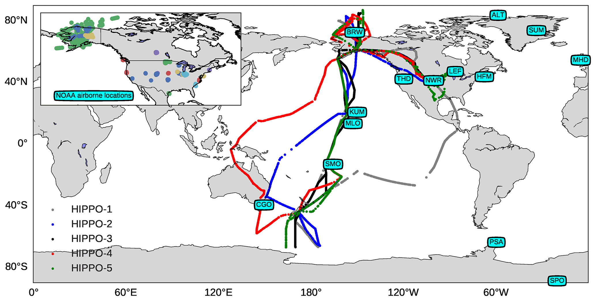
Figure 1 Geographical locations of the NOAA ground-based observations (shown in boxes), the five HIPPO campaign tracks and the NOAA profile programme (inset). Note that there are no NOAA surface stations located in Asia, South America or Africa.

2.1.2 HIPPO aircraft and NOAA airborne data

Flask data of the HIAPER Pole-to-Pole Observations (HIPPO) experiments (Wofsy, 2011; Wofsy et al., 2017) are used to validate the results of the inverse modelling. There were five HIPPO campaigns conducted from 2009 to 2011 that sampled the COS mole fraction from the North Pole to the South Pole and from the lower troposphere up to the stratosphere. Three different instruments were used to make measurements of COS during HIPPO. Instrument 2 was used by NOAA to measure COS, and instrument 1 was calibrated consistently with the NOAA calibration standard. Results of instrument 3 were scaled to be consistent with those of instrument 2, such that results from all three instruments on HIPPO are referenced to the same NOAA scale. The probability distribution function of the mole fractions confirms that the three instruments report consistent values, with similar averages (see Fig. S1). Thus, HIPPO data provide valuable data to check the consistency of the optimized COS budget. The flight routes of the five campaigns are shown in Fig. 1. In some numerical experiments, HIPPO data are additionally assimilated to investigate their impact on the optimized COS budget. To investigate this impact on the vertical distribution of COS, we compared model results to 2008–2011 NOAA airborne data that are mainly available over North America (Fig. 1). The number of aircraft sites used is 19, and the upper altitude that was typically reached is 8 km.

2.1.3 Satellite data

Our inverse modelling results are compared to three independent satellite data sources: TES-Aura, the Atmospheric Chemistry Experiment Fourier Transform Spectrometer (ACE-FTS) and the Michelson Interferometer for Passive Atmospheric Sounding (MIPAS). We have selected the period 2008–2011 for the comparison.

NASA's TES is both a nadir- and a limb-viewing instrument that flies on the Aura satellite, which was launched in 2004 (Beer et al., 2001). TES measures the infrared radiation emitted from the Earth and atmosphere in a high spectral resolution for 16 orbits every other day. From these spectra, abundances of tropospheric trace gases are retrieved. The COS product used in this study is described in Kuai et al. (2014). The COS retrievals cover the whole vertical column, have less than 1^∘ of freedom (DOF) and show maximum sensitivity in the 300–500 hPa region. We will therefore focus our comparisons on total COS columns. To account for the non-uniform vertical sensitivity, we use the averaging kernel (AK) in the model–satellite comparison. As described in Kuai et al. (2014), the AK included in the TES data files is defined in log space and should be applied as

$$\begin{array}{}\text{(1)}& \ln \left({\mathit{\chi }}_{\mathrm{con}}\right)=\ln \left({\mathit{\chi }}_{\mathrm{p}}\right)+\mathbf{A}\left[\ln \right({\mathit{\chi }}_{\mathrm{m}})-\ln ({\mathit{\chi }}_{\mathrm{p}})+\mathit{\beta }],\end{array}$$

where χ_con, χ_p and χ_m are the convolved, prior and modelled profiles, respectively, and A is the AK. β is a global constant bias correction term. In Kuai et al. (2015) a β value of 0.2 was derived using inverse modelling, partly to account for the missing stratospheric decay in that study. In Sect. 3.4 the modelled profiles are convolved with the TES AK (χ_con), vertically integrated, and compared to the TES columns.

ACE-FTS is a high-spectral-resolution infrared Fourier transform spectroscopy instrument that performs solar occultation measurements, with the aim of sampling stratospheric and upper tropospheric profiles of trace gases (Boone et al., 2013). The instrument flies on SCISAT, a Canadian satellite mission for remote sensing of the Earth's atmosphere that was launched in 2003. Its orbit covers tropical, mid-latitude and polar regions. COS is one of the atmospheric trace gases measured by the ACE-FTS instrument (Koo et al., 2017). ACE-FTS profiles have been compared to balloon observations and have generally shown good agreement, with underestimations smaller than 20 % (Krysztofiak et al., 2015). We use product version 3.6, and only observations with a quality flag of zero are used. ACE-FTS measures COS within 0–150 km vertically, but the data quality is only sufficient in the upper troposphere and lower stratosphere (UTLS).

MIPAS is a Fourier transform spectrometer for detection of the radiative emission of various molecules in limb observation mode in the middle and upper atmosphere (Fischer et al., 2008). MIPAS flew on ESA's Envisat platform that operated between 2002–2012. MIPAS delivers global atmospheric COS profiles in the upper troposphere and stratosphere (Glatthor et al., 2015, 2017). Similarly to TES, the MIPAS data product contains representative AKs and prior profiles to facilitate comparison to modelled profiles but not in log space, since MIPAS COS is evaluated by a linear retrieval:

$$\begin{array}{}\text{(2)}& {\mathit{\chi }}_{\mathrm{con}}={\mathit{\chi }}_{\mathrm{p}}+\mathbf{A}[{\mathit{\chi }}_{\mathrm{m}}-{\mathit{\chi }}_{\mathrm{p}}],\end{array}$$

where χ_m has to be resampled on the MIPAS retrieval grid in advance.

As for most other gases, the prior profile for MIPAS COS retrievals is a zero profile. Equation (2) thus becomes a simple multiplication of the AK with the modelled profiles. A detailed description of the application of MIPAS AKs on other data sets can be found in Stiller et al. (2012).

The MIPAS product has been compared to modelled COS distributions (Glatthor et al., 2015) and ACE-FTS (Glatthor et al., 2017). The latter comparison showed that MIPAS retrieves higher mole fractions around the tropopause compared to ACE-FTS. The MIPAS product has also been compared to airborne measurements of the HIPPO, ARCTAS and INTEX-B campaigns (Supplement of Glatthor et al., 2015). Finally, MIPAS has been compared to MkIV and SPIRALE profiles (Glatthor et al., 2017).

The retrievals of TES, MIPAS and ACE-FTS v3.6 are provided on 14, 60 and 150 vertical levels in the atmosphere, respectively. We map our modelled COS profiles to these levels using a mass-conserving interpolation scheme.

2.1.4 Seasonal decomposition

In Sect. 3.1 we apply a simple seasonal decomposition method to our calculated exchange fluxes. The seasonal decomposition is performed using the Python module statsmodels, version 0.10. The time series are decomposed into trend, seasonality and noise:

$$\begin{array}{}\text{(3)}& \mathit{y}\left(t\right)={\mathit{y}}_{\mathrm{t}}\left(t\right)+{\mathit{y}}_{\mathrm{s}}\left(t\right)+{\mathit{y}}_{\mathrm{r}}\left(t\right),\end{array}$$

with y(t) being the monthly exchange fluxes and y_t, y_s and y_r the trend, seasonal and residual components, respectively.

2.2 Model description

2.2.1 Anthropogenic emissions

We have implemented the anthropogenic emissions based on a recent global gridded emission inventory of COS (Campbell et al., 2015; Zumkehr et al., 2018). Since we were aiming to model COS, CS₂ and DMS as separated tracers, we disentangled the reported COS emissions into COS and CS₂ contributions. Here, we applied an assumed yield of 0.87 (Zumkehr et al., 2018), which means that 1 mol of CS₂ yields 0.87 mol of COS. As a precursor of COS, CS₂ reacts with OH to produce COS and has an atmospheric lifetime of about 12 d (Khalil and Rasmussen, 1984). We applied a detailed anthropogenic emission budget for COS and CS₂ from Table 1 in Lee and Brimblecombe (2016). This allows us to roughly estimate the ratio of this budget and hence the direct and indirect COS anthropogenic emissions. The converted emissions averaged over the period 2000–2012 are summarized in Table 1.

The total anthropogenic COS emissions are on average 343.3 Gg a⁻¹, split between direct COS emissions of 147.5 Gg a⁻¹ and CS₂ emissions of 450.2 Gg a⁻¹. This indicates that CS₂ is an important precursor of COS. Figure 2 shows time series of COS and CS₂ anthropogenic emissions. COS emissions are dominated by industrial and residential coal sources, while CS₂ emissions are dominated by rayon industry and TiO₂ production. Moreover, while COS emissions remained relatively constant in the 2007–2012 period, CS₂ emissions showed an increasing trend.

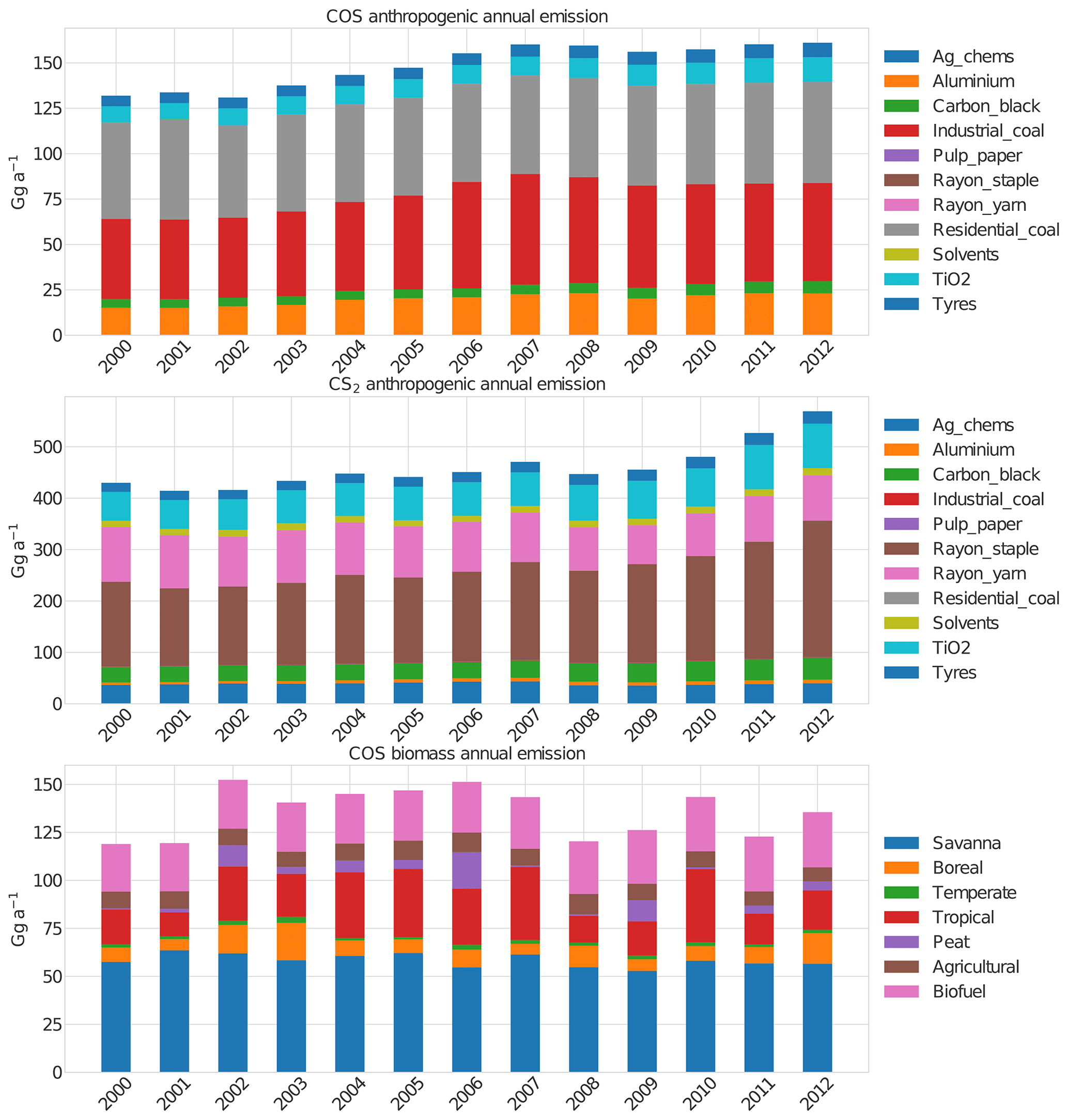
Figure 2 Yearly anthropogenic emissions of COS and CS₂ as well as COS biomass burning emissions in the period 2000 to 2012. We disentangled the emissions reported in Zumkehr et al. (2018) into COS and CS₂ emissions using their reported yield of 0.87 (see main text). Biomass burning emissions are calculated based on the GFED V4.1 biomass burning inventory and the CEDS biofuel emission inventory (see main text).

While Zumkehr et al. (2018) assumed a molar yield of CS₂ to COS of 87 %, other reported yields are (83 ± 8) % (Stickel et al., 1993) and 81 % (Chin and Davis, 1993). We decided to use a yield of 83 % in our modelling, while we used the reported yield of 87 % to produce the numbers listed in Table 1. This implies that we introduce slightly less COS into the atmosphere compared to using the Zumkehr et al. (2018) data as direct COS emissions. Note that we apply all categorical emissions or fluxes with a monthly time resolution. It is also worth noting that the uncertainty in the anthropogenic inventory is much larger than the uncertainty in molar yield.

2.2.2 Biomass burning emissions

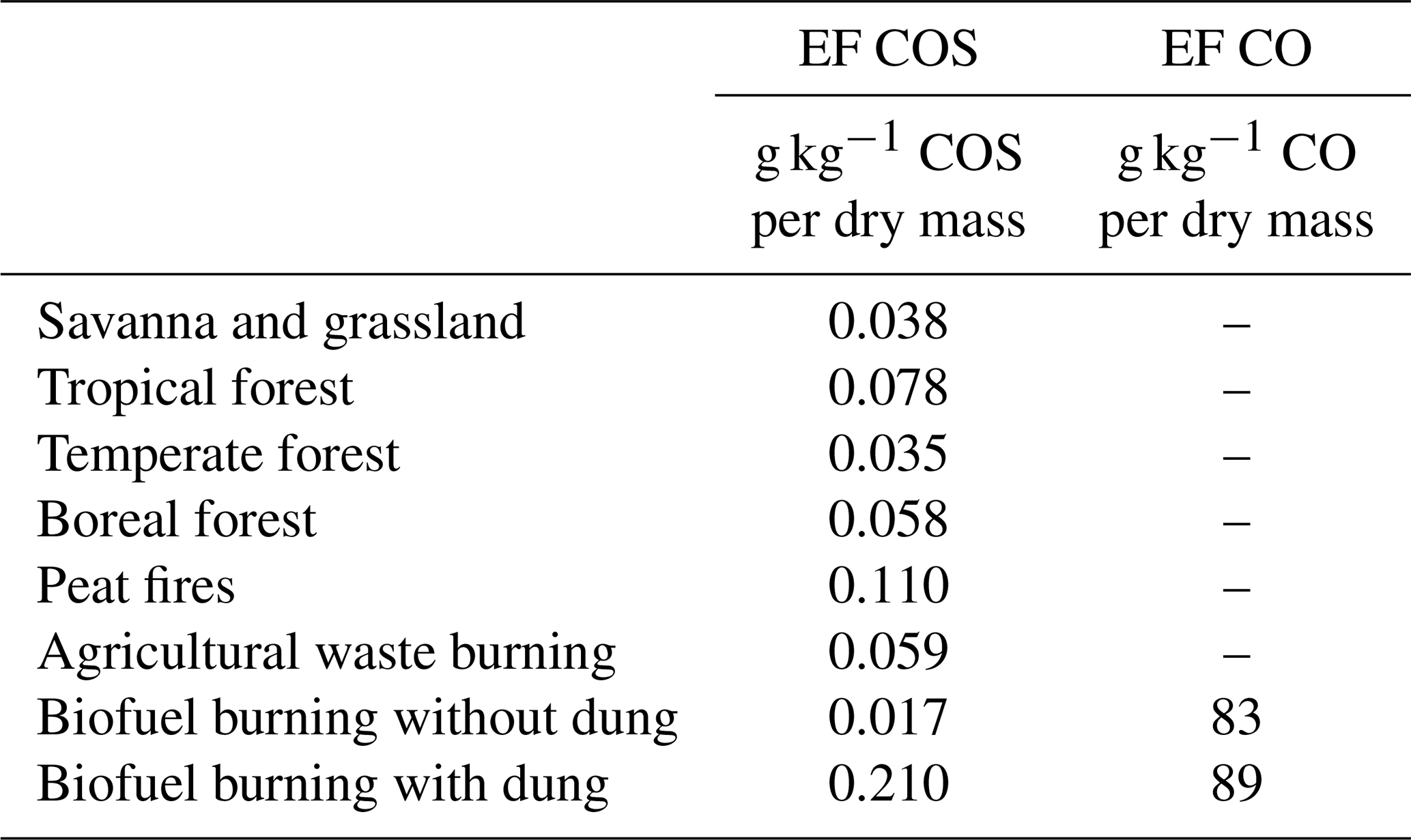
We estimated biomass burning emissions based on the widely used GFED V4.1 data set (Randerson et al., 2018) for six of the seven emission categories listed in Table 2. In converting dry mass burned to COS emissions, we used the updated emission factors reported in Andreae (2019). For biofuel use, we base our estimates on the Community Emissions Data System (CEDS) (Hoesly et al., 2018). We calculated COS emissions by first converting CO emissions to dry mass burned, which was converted to COS emissions in a second step. Emission factors are listed in Table 2. In this process we made a distinction between biofuel with and without dung. Dung burning is mainly employed in southern Asia (Fernandes et al., 2007), and we applied the dung emission ratios only in the region 0–40^∘ N and 60–100^∘ E. Our biomass burning emissions in the 2000–2012 period are in the range of 118–154 Gg a⁻¹ (Fig. 2) and similar to the emissions used in Berry et al. (2013) (135 Gg a⁻¹) and estimates reported in Campbell et al. (2015) (116 ± 52 Gg a⁻¹). The more recent biomass burning estimate from Stinecipher et al. (2019) based on GFED 1997–2016 data reports global emissions of 60 ± 37 Gg a⁻¹. Note, however, that biofuel use is not included in this estimate. The spatial and seasonal distribution of the biomass burning emissions averaged over the period 2000–2012 is presented in Fig. S2 in the Supplement.

Table 2 Biomass burning emission factors used in converting COS emissions. EF COS denotes the COS emission factor from dry mass in units of g kg⁻¹ COS per dry mass, and EF CO denotes the CO emission factor in g kg⁻¹ CO per dry mass. Emission factors were taken from Andreae (2019).

2.2.3 Biosphere flux

Our biosphere fluxes are based on simulations with the Simple Biosphere Model, version 4 (SiB4) (Berry et al., 2013; Haynes et al., 2019). Currently, soil uptake is scaled to the CO₂ soil respiration term, and the implementation of specific COS soil models (Sun et al., 2015; Ogée et al., 2016) is ongoing. SiB4 was constrained by a prescribed COS mole fraction of 500 pmol mol⁻¹ outside the canopy. This 500 pmol mol⁻¹ is merely a placeholder and probably leads to too large fluxes over the active biosphere, where COS mole fractions decline because of strong uptake. This is further discussed in Sect. 3.5. Meteorological data that are used as forcing for SiB4 are taken from the Modern-Era Retrospective Analysis for Research and Applications (MERRA) and are available from 1980 onwards (Rienecker et al., 2011). A spin-up of the model was performed for the period 1850–1979 to reach an equilibrium of the carbon pools. As no MERRA data were available for the spin-up period, the climatological average of MERRA data over the period 1980–2018 was used as meteorological input for the spin-up period. A final simulation was performed for 1980–2018 with the actual MERRA driver data. The 2000–2018 average flux to the biosphere (vegetation plus soil) amounts to −1053 Gg a⁻¹, in line with estimates of −951 Gg a⁻¹ using SiB3 (Kuai et al., 2015; Berry et al., 2013). The spatial and seasonal distribution of the biosphere uptake is shown in Fig. S3. The uptake shows a large seasonal cycle in the NH and large uptake over tropical forests. The biosphere fluxes were deployed on a monthly timescale.

2.2.4 Ocean emissions

Climatological ocean emissions of COS and the COS precursors CS₂ and DMS are based on Suntharalingam et al. (2008) and Kettle et al. (2002). Large quantities of COS, DMS and CS₂ are emitted from open oceans. The estimated DMS emissions are about 22 Tg a⁻¹, and we note that even if the COS yield from oxidation of DMS is as small as 0.7 % (Barnes et al., 1996), 156 Gg a⁻¹ COS has already been formed. The CS₂ direct emissions from oceans are roughly 195 Gg a⁻¹, yielding 81 Gg a⁻¹ of COS. When the ocean water is cold enough, oceans can turn into a sink of COS instead of a source (Lennartz et al., 2017). Figure S4 shows the spatial distribution of the January and July direct and indirect ocean emissions of COS. Note that our estimate of all COS oceanic emissions as 277 Gg a⁻¹ is substantially smaller than the estimate of 813 Gg a⁻¹ by Launois et al. (2015).

Figure 3 Error analysis for NOAA stations. Black error bars represent the time variations in the errors over a 3-year period (2008–2010). For ALT, SPO and SUM, the flux-related errors are close to zero and not shown. Stations are ordered from the North Pole to the South Pole.

2.3 TM5-4DVAR inverse modelling system

We have implemented three tracers (COS, CS₂ and DMS) in the inverse modelling framework TM5-4DVAR (Krol et al., 2005, 2008; Meirink et al., 2008). In brief, the TM5 model is used to convert fluxes, collected in state vector x, to observations y:

$$\begin{array}{}\text{(4)}& \mathit{y}=\mathit{H}\mathbf{\left(}\mathit{x}\mathbf{\right)},\end{array}$$

where H represents the global chemistry transport model TM5. Since the relation between fluxes and observations is currently linear, y=H(x) can be written as y=Hx. In a flux inversion a cost function is minimized. The cost function has the following form:

$$\begin{array}{}\text{(5)}& \begin{array}{rl}J\left(\mathit{x}\right)& ={\displaystyle \frac{\mathrm{1}}{\mathrm{2}}}(\mathit{x}-{\mathit{x}}_b{)}^T{\mathbf{B}}^{-\mathrm{1}}(\mathit{x}-{\mathit{x}}_b)\\ & +{\displaystyle \frac{\mathrm{1}}{\mathrm{2}}}(\mathit{y}-\mathit{H}\mathit{x}{)}^T{\mathbf{R}}^{-\mathrm{1}}(\mathit{y}-\mathit{H}\mathit{x}),\end{array}\end{array}$$

where x_b represents the prior state of the fluxes and B and R are the error covariance matrices of the fluxes and observations, respectively. B contains the errors assigned to the fluxes, as well as their correlations in space and time (i.e. B is a non-diagonal matrix). R contains the errors assigned to (y−Hx). These errors are assumed to be uncorrelated and they also include, besides the observational errors, errors related to the process of mapping coarse-scale fluxes x to localized observations y. The adjoint of the TM5 model (Krol et al., 2008; Meirink et al., 2008) is used to calculate the gradient of this cost function with respect to all elements in the state vector:

$$\begin{array}{}\text{(6)}& \mathrm{\nabla }J\left(\mathit{x}\right)={\mathbf{B}}^{-\mathrm{1}}(\mathit{x}-{\mathit{x}}_b)+{\mathit{H}}^T{\mathbf{R}}^{-\mathrm{1}}(\mathit{H}\mathit{x}-\mathit{y}).\end{array}$$

Table 3 Names and error settings of the inversions performed in this study. The values correspond to grid-scale errors. Monthly flux fields are optimized using spatial and temporal correlation lengths of 4000 km and 12 months, except for inversion S_u, in which multiple settings are explored.

In all inversions, y is represented by COS observations from the NOAA flask network data (Montzka et al., 2007). Our flux space, however, in addition to COS emissions, may represent CS₂ and DMS emissions from anthropogenic activity and oceans. To map their influence on simulated COS observations y, we need to consider chemical conversions of CS₂ and DMS to COS. CS₂ and DMS are short-lived trace gases, with atmospheric lifetimes of approximately 12 d (Khalil and Rasmussen, 1984) and 1.2 d (Khan et al., 2016; Boucher et al., 2003; Breider et al., 2010), respectively. For CS₂ we implemented OH-initiated conversion to COS, while for DMS we simply apply exponential decay with a lifetime of 1.2 d. COS itself is also destroyed by OH in the troposphere and by photolysis in the stratosphere. For OH, we use monthly varying climatological OH fields (Spivakovsky et al., 2000) and apply a correction factor of 0.92 (Naus et al., 2019). In summary, the chemistry that is implemented therefore consists of the following four reactions:

$$\begin{array}{}\text{(R1)}& {\displaystyle }\mathrm{COS}+\mathrm{OH}\stackrel{r_{\mathrm{1}}}{⟶}\mathrm{products},\text{(R2)}& {\displaystyle }\mathrm{COS}+\mathrm{h}\mathit{\nu }\stackrel{j_{\mathrm{1}}}{⟶}\mathrm{products},\text{(R3)}& {\displaystyle }{\mathrm{CS}}_{\mathrm{2}}+\mathrm{OH}\stackrel{r_{\mathrm{2}}}{⟶}{f}_{\mathrm{1}}\mathrm{COS}+\mathrm{other}\mathrm{products},\text{(R4)}& {\displaystyle }\mathrm{DMS}\stackrel{r_{\mathrm{3}}}{⟶}{f}_{\mathrm{2}}\mathrm{COS}+\mathrm{other}\mathrm{products},\end{array}$$

where j₁ is the stratospheric photolysis frequency and r₁ and r₂ are the rate constants of COS and CS₂ OH oxidation, respectively. The fractions f₁ and f₂ represent the molar yields of COS from CS₂ (taken as 0.83; Stickel et al., 1993) and DMS (taken as 0.007; Barnes et al., 1996). The rate r₁ is calculated according to the Arrhenius equation:

$$\begin{array}{}\text{(7)}& r_{\mathrm{1}}=A{e}^{\frac{-\mathrm{1200}\text{K}}{T}},\end{array}$$

where T is temperature in kelvins and A is $\mathrm{1.13}\times {\mathrm{10}}^{-\mathrm{12}}$ cm³ s⁻¹ molecule⁻¹ (Cheng and Lee, 1986). The rate r₂ is $\mathrm{2.0}\times {\mathrm{10}}^{-\mathrm{12}}$ cm³ s⁻¹ molecule⁻¹ (Jones et al., 1983). Note that this rate expression is independent of temperature and slightly different from that of Sander et al. (2006). This latter rate was used in Khan et al. (2017) and resulted in a short CS₂ lifetime of 2.8–3.4 d. However, when we implement the rate of Sander et al. (2006) in TM5, we find a CS₂ lifetime of 6.2 d. This might be due to the fact that we ignore CS₂ deposition (15 % of the loss according to Khan et al., 2017) or that we use lower OH or higher emissions. Rate $r_{\mathrm{2}}=\mathrm{2.0}\times {\mathrm{10}}^{-\mathrm{12}}$ cm³ s⁻¹ molecule⁻¹ leads to an atmospheric CS₂ lifetime of 9.4 d in TM5. Rate r₃ represents an exponential decay of 1.2 d for DMS ($r_{\mathrm{3}}=\mathrm{9.6}\times {\mathrm{10}}^{-\mathrm{6}}$ s⁻¹).

COS photolysis frequencies are calculated based on a troposphere ultraviolet and visible (TUV) radiation model (Madronich et al., 2003). Based on monthly climatologies of ozone profiles and temperatures, monthly averaged photolysis frequencies are calculated on a 1 km grid spanning 0–120 km and on 180 latitude bands. Implemented in TM5, COS loss in the stratosphere amounts to about 40 Gg a⁻¹. This estimate is in line with earlier estimates of (50 ± 15) Gg a⁻¹ (Brühl et al., 2012; Barkley et al., 2008; Chin and Davis, 1995; Engel and Schmidt, 1994; Weisenstein, 1997; Krysztofiak et al., 2015; Turco et al., 1980; Crutzen and Schmailzl, 1983; Crutzen, 1976).

2.4 Model–data mismatch errors

The diagonal elements of the error covariance matrix R in Eq. (5) contain contributions from observational errors, representation errors and errors related to applying large fluxes in the planetary boundary layer (Bergamaschi et al., 2010):

$$\begin{array}{}\text{(8)}& {\mathit{\sigma }}_{\mathrm{t}}=\sqrt{({\mathit{\sigma }}_{\mathrm{o}}^{\mathrm{2}}+{\mathit{\sigma }}_{\mathrm{r}}^{\mathrm{2}}+{\mathit{\sigma }}_{\mathrm{f}}^{\mathrm{2}})},\end{array}$$

where σ_t is the total error, σ_o the observational error, σ_r the representation error and σ_f an error related to applying large surface fluxes. The assumed observational error is shown in Fig. 3. It is worth noting that observational errors are usually overwhelmed by the representation and flux errors. The representation error is calculated by sampling the modelled gradients in the vicinity of the sampled station (Bergamaschi et al., 2010). Finally, the flux error in each cell is linked to the magnitude of the monthly surface flux f (kg m⁻² s⁻¹ in each cell) applied in the model as

$$\begin{array}{}\text{(9)}& {\mathit{\sigma }}_{\mathrm{f}}={\displaystyle \frac{fg{M}_{\mathrm{air}}\mathrm{\Delta }t}{M_{\mathrm{S}}\mathrm{\Delta }p}}.\end{array}$$

Here, f represents the sum of all COS prior flux components. In this sum, the biosphere flux is dominant over regions with strong biosphere uptake. Further, g is gravitational acceleration (9.8 m s⁻²), M_air is the molar mass of dry air (28.9 kg kmol⁻¹), M_S is the molar mass of sulfur (32.1 kg kmol⁻¹), Δp (Pa) is the thickness of the first model layer and Δt is the time (s) over which the COS flux accumulates (we use 1 h). Note that σ_f is unitless and is multiplied by 1×10¹² to obtain units of pmol mol⁻¹.

Based on the total error, we define a χ² metric to quantify how well the observations are reproduced by the model (e.g. at a particular station).

$$\begin{array}{}\text{(10)}& {\mathit{\chi }}^{\mathrm{2}}={\displaystyle \frac{{\sum }_{i=\mathrm{1}}^N(\mathit{H}\mathit{x}-\mathit{y}{)}^{\mathrm{2}}}{N{\mathit{\sigma }}_{\mathrm{t}}^{\mathrm{2}}}},\end{array}$$

where N is the number of individual observations. We can calculate this metric before optimization (prior) and after optimization (posterior). χ² is used to diagnose whether inversions are over-fitting or under-fitting the information contained in the measurement network. A value of χ²≈1.0 indicates that the inverse system is able to fit the data within the error setting (Hooghiemstra et al., 2011). A large posterior χ² indicates that the state does not have enough degrees of freedom to fit the observations properly (or the error settings are too small). A small posterior χ² indicates over-fitting of the observations (or too wide error settings).

2.5 Model settings

In this study, the TM5-4DVAR system is employed on a global resolution of ${\mathrm{6}}^{\circ }\times {\mathrm{4}}^{\circ }$ (longitude × latitude). Flux fields are coarsened from a resolution of ${\mathrm{1}}^{\circ }\times {\mathrm{1}}^{\circ }$. To create a reasonable start field for the inversions, we initially performed an 11-year forward simulation starting with zero initial mole fractions and baseline surface fluxes augmented by 432 Gg a⁻¹, distributed uniformly to close a gap in the global budget. After 11 years, sources and sinks are roughly in balance, with atmospheric mole fractions of about 500 pmol mol⁻¹. Note that fluxes are used as zero-order terms, while the COS removal by OH and photolysis are first-order removal terms that grow as the atmospheric COS increases.

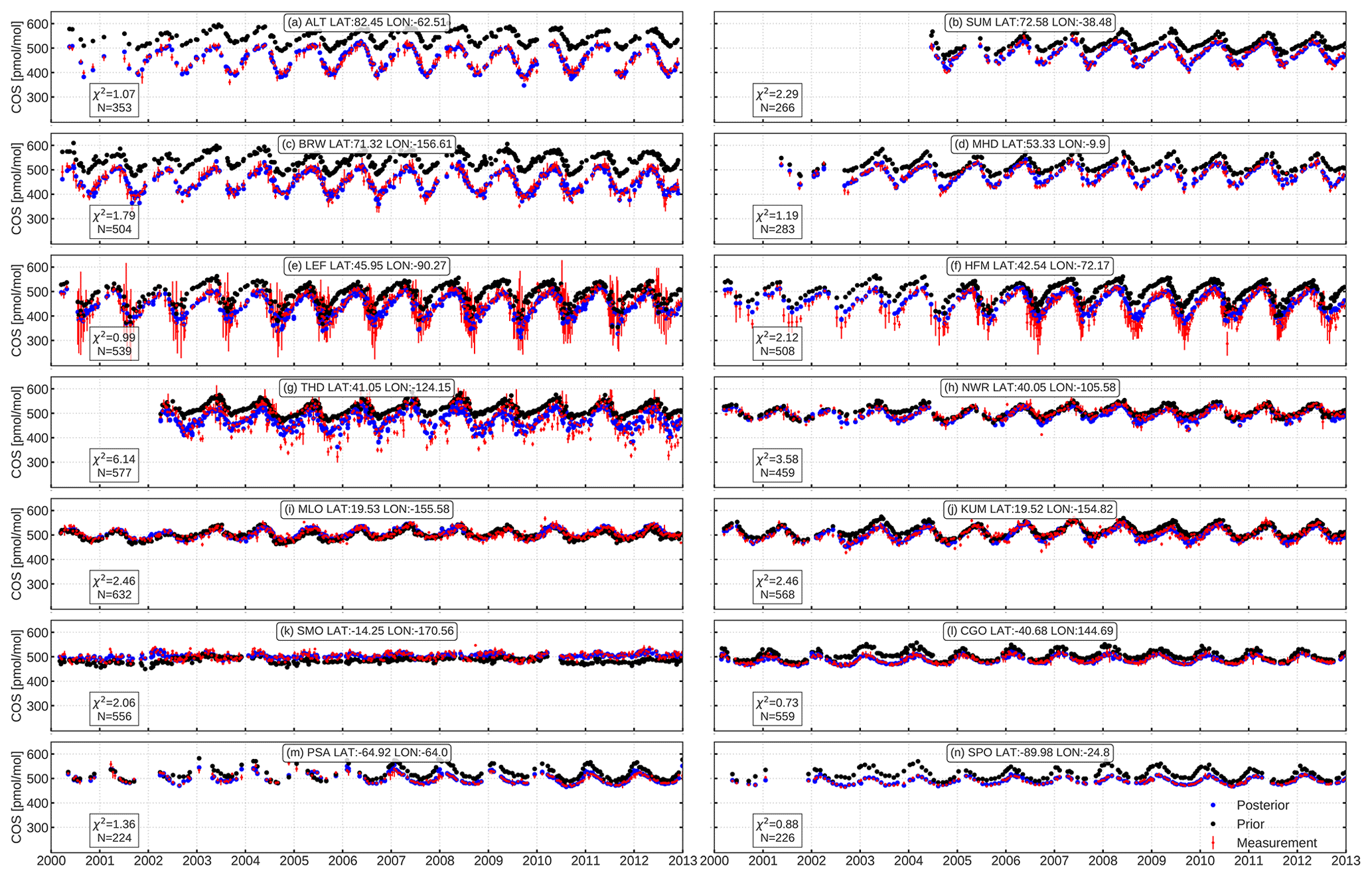
Figure 4 COS prior and posterior comparison at NOAA stations. Red dots and bars are NOAA measurements with errors. Blue and black dots represent the posterior and prior simulation, respectively. Results are shown for inversion S_u in which only the unknown emission category is optimized.

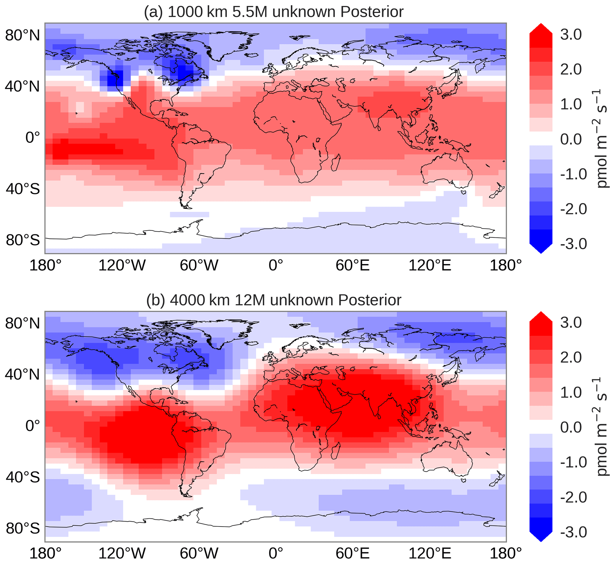
Figure 5 Optimized emission pattern of the unknown field of inversion S_u for different settings of the spatio-temporal correlation lengths. (a) Spatial correlation of 1000 km and temporal correlation of 5.5 months. (b) Spatial correlation of 4000 km and temporal correlation of 12 months. Results are averages over 2008–2011.

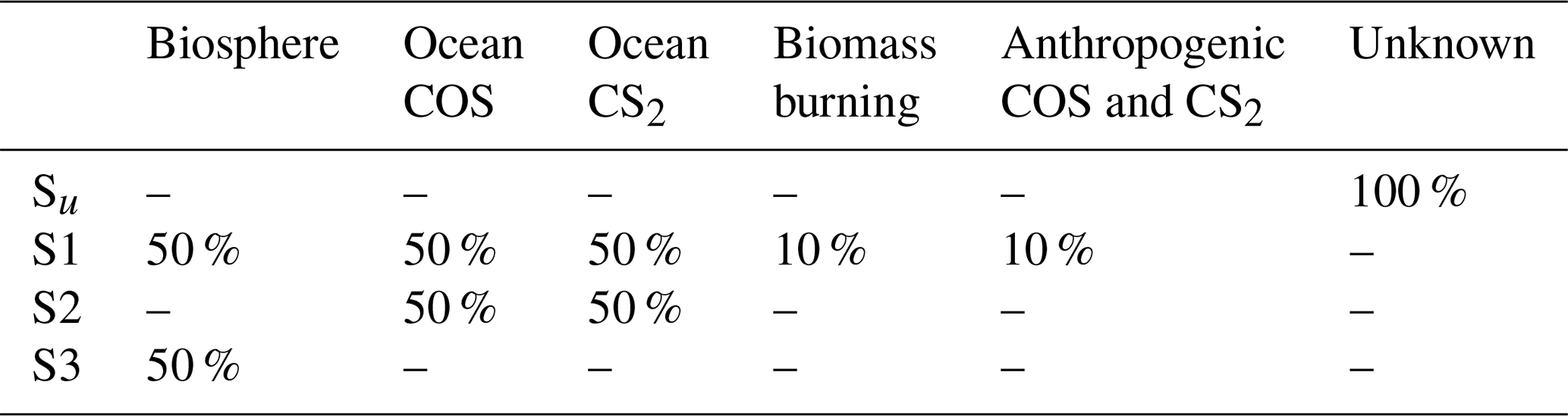
We will present the results of four inversions. Firstly, we optimized the missing emissions, which amount to 432 Gg a⁻¹. This inversion will be denoted by S_u throughout the paper. The aim of this inversion is to investigate the spatial structure and temporal variability in the missing COS emissions. This is the first time that a formal 4DVAR approach is applied to the COS budget. To this end, we start from an emission field of 432 Gg a⁻¹ that is uniformly distributed globally. We optimize emissions on a monthly timescale and assign a grid-scale prior error of 100 %, which is an arbitrary number to give fluxes enough freedom to adjust. In a 3-year inversion, the total number of state vector elements amounts to 97 200 (36 months × 45 latitudinal bins × 60 longitudinal bins). The total number of NOAA observations is much smaller, thus rendering the inversion under-determined. We therefore also use inversion S_u to explore different settings of the temporal and spatial correlation lengths, which control the degrees of freedom of the state vector. We explore spatial correlation lengths of 1000, 4000, 6000, 10 000 and 20 000 km and temporal correlation lengths of 5.5, 7, 9.5 and 12 months.

Secondly, we explore the optimization of specific categories in inversions S1–S3. In S1 we attempt to perform an “objective” inversion, in which we assign grid-scale errors of 50 % to the biosphere and ocean (we optimize both COS and CS₂) and 10 % to the anthropogenic COS and CS₂ emissions and to the biomass burning emissions. Furthermore, in S2 we only optimize ocean exchange and in S3 we only optimize the biosphere exchange. The aim of inversions S1–S3 is to explore whether either ocean fluxes or the biosphere fluxes (or both) should be used to close the gap in the COS budget. Note that DMS ocean emissions are not optimized. The names and settings of the inversions are summarized in Table 3.

The cost function is minimized with CONGRAD, an efficient numerical algorithm for solving linear systems (Lanczos, 1950). This minimizer has also been used in previous inverse modelling studies with the TM5-4DVAR system (Basu et al., 2013; Monteil et al., 2011, 2013; Houweling et al., 2014; Pandey et al., 2015). For convergence, we request a gradient norm reduction of 1 × 10⁵, and this reduction is usually achieved within 40 iterations.

We perform flux inversions for the period 2000–2012. To decrease computational costs, we adopt the strategy to run parallel 3-year inversions, and we discard the optimized fluxes of the first 6 months (spin-up) and the last 6 months (spin-down). For example, the first inversion targets the period 1 January 2000 to 1 January 2003, the second inversion 1 January 2002 to 1 January 2005 and so on. In the spin-up period the fluxes in the first 6 months are used to adjust the imperfect initial condition. In the spin-down period, fluxes are less reliable, because they have not been well constrained by observations. The optimized fluxes in the overlapping years are used to check the inversion results for consistency. In general, it is found that the optimized fluxes in the overlapping periods are highly consistent.

3 Results

3.1 Closing a gap in the COS budget

In this section, we consider inversion S_u, in which a uniform field emitting 432 Gg a⁻¹ is optimized. We use different settings for the spatial and temporal correlation lengths of this field in the inversion and quantify the posterior goodness of fit using the χ² metric (Eq. 10). As presented in more detail in Fig. S5 we find, as expected, that χ² decreases with increasing degrees of freedom (smaller correlations).

Overall, the posterior fit to NOAA surface observations from 14 sites does not improve significantly for smaller correlation lengths. If we analyse the posterior fit to the short-term sampling programme from HIPPO, however, we find that the χ² reaches a minimum (see Fig. S5). After this minimum, χ² values increase again, a possible sign of over-fitting. We therefore select 4000 km and 12 months for the spatial and temporal correlation length, respectively, and use these values in the remainder of this study.

Figure 4 presents the fit to observations of the prior and posterior simulation, for the inversion with temporal and spatial correlation lengths of 12 months and 4000 km, respectively. Corresponding χ² metrics per station are listed as labels in Fig. 4. Posterior fits are by design much better than prior fits. Only for NOAA stations THD and NWR does the posterior χ² remain larger than 3, indicating insufficient degrees of freedom to resolve remaining discrepancies, underestimated model errors or the influence of outliers (see Fig. 4g, h). THD is a coastal site (107 m a.s.l.), and NWR is a tundra site above the treeline (3526 m a.s.l.) in the USA (Fig. 1), and thus the model resolution of 6${}^{\circ }\times$4^∘ is likely too coarse to represent these sites. The local coastal effect might be another reason why THD yields a larger χ² (Riley et al., 2005). It is worth noting that the posterior simulation does not exhibit jumps in overlapping years from the parallel-running inversions, indicating that our inversion strategy works well.

The correlation settings have a large impact on the optimized fluxes. Figure 5 shows the spatial distribution of the posterior flux field calculated with two different correlation settings. For correlations of 1000 km and 5.5 months (panel a) we detect a typical pattern that signals over-fitting of the observations. In such a pattern, the optimized flux displays hot spots close to measurement locations (e.g. THD, MLO, SMO). For very long spatial correlations, e.g. 20 000 km, posterior fits are poor (χ²>6; see Fig. S5) and optimized flux patterns show irregular behaviour (Fig. S6). Our best inversion (4000 km and 12 months) produces a smooth optimized flux without apparent spatial patterns near observational stations (Fig. 5b). This pattern confirms the missing COS sources in the tropics (Suntharalingam et al., 2008; Berry et al., 2013) and also requires more uptake at high latitudes, especially in the NH.

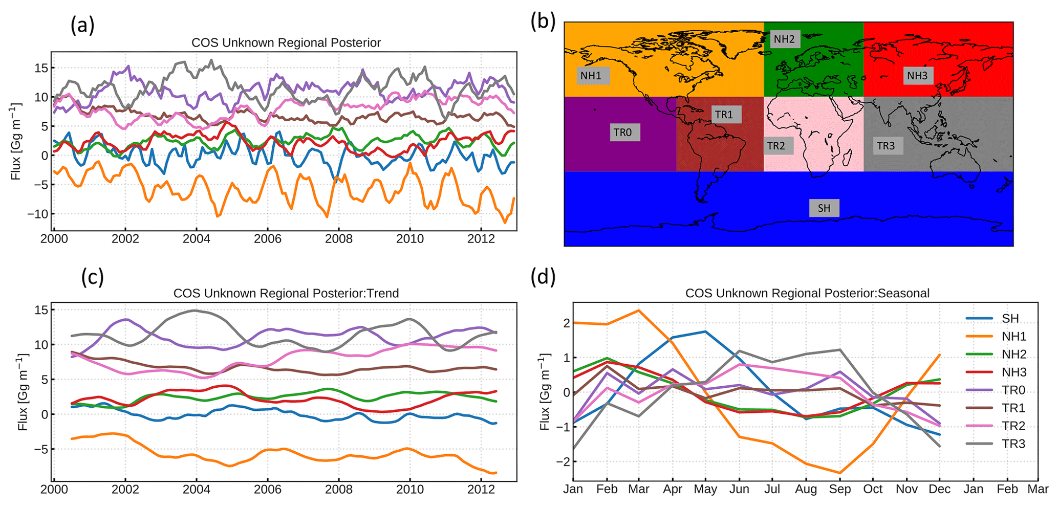
Figure 6 Regional analysis of multi-year optimized COS fluxes of inversion S_u: (a) posterior flux per region, (b) regions over which the posterior flux is analysed, (c) trend in the decomposed signal and (d) seasonal signal in the decomposed signal. Note that region colours in (b) are used in (a), (c) and (d).

To investigate the variation in the optimized fluxes of inversion S_u, we decompose the flux components as described in Sect. 2.1.4. The monthly fluxes and derived long-term trend are shown in Fig. S7. The global flux was subsequently split into eight regions, and the regional COS S_u fluxes analysed for these regions are shown in Fig. 6. Region NH1 (North America plus part of the Pacific and Atlantic oceans, orange) shows a negative “unknown” flux, indicating that more sinks are needed. This likely points to an underestimation of the biosphere uptake in the prior, since this region (that is well constrained by observations) depicts a clear seasonal cycle in the optimized unknown flux.

A larger sink is also needed in NH2 (Europe, green) and NH3 (Asia, red) but one of smaller magnitude than in NH1. Tropical regions TR0–TR3 have a similar trend and seasonality and generally show a positive flux signal, with a small seasonal cycle. This could represent an oceanic signal (underestimated emissions of COS or COS precursors in the prior), a signal from biomass burning or an overestimated biosphere sink. The ocean-dominated region SH (blue) has a near-neutral flux, with a seasonal cycle that shows higher emissions in local autumn and early winter. In the next section, we will explore the optimization of the ocean and biosphere fluxes.

Table 4 Results from inversions S_u, S1, S2 and S3 compared to published global COS budgets. The total sources, total sinks, the unknown flux and the total flux are shown in italics.

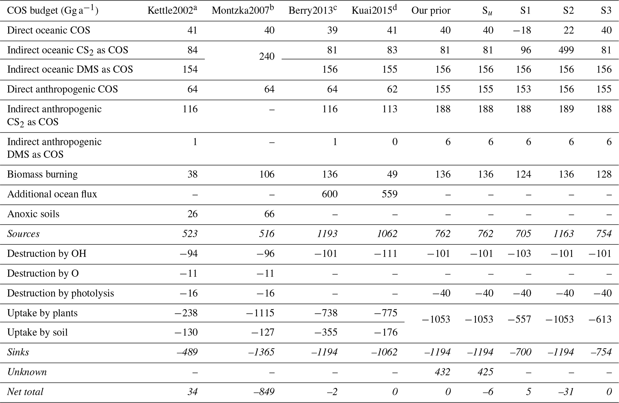
^a Kettle et al. (2002). ^b Table 2 from Montzka et al. (2007). ^c Berry et al. (2013). ^d Kuai et al. (2015).

3.2 Objective inversions

In this section we will discuss the results of inversions S1, S2 and S3. The resulting global budgets are compared to literature values in Table 4. In addition, χ² metrics and biases of the various inversions are reported in Table 5 for the NOAA surface network, the HIPPO campaigns and the NOAA airborne profiles. Note that we also report results for optimizations that assimilated the HIPPO observations besides the NOAA surface data. The period of the analysed inversions is 2008–2010. The prior and posterior emission errors and error reduction in the different inversion scenarios are listed and discussed in Table S1.

The three inversions are all able to close the gap in the global COS budget with, however, very different budget terms (Table 4). Inversions S1 and S3 close the gap in the budget by a drastic reduction in the biosphere uptake in the tropics and more biosphere uptake at high latitudes. When the biosphere is not optimized (S2), the inversion enhances the CS₂ tropical oceanic source and reduces direct COS emissions from the high-latitude oceans (Table 4). Both patterns lead to reduced tropical biospheric uptake and more uptake at high latitudes, as was found for inversion S_u.

Concerning the posterior fit to observations, none of the S1–S3 inversions performed like inversion S_u. The statistics in Table 5 show that S_u leads to the best fit to the assimilated observations and only a small remaining bias. Inversions S1 and S3 show better χ² statistics and smaller biases than inversion S2, because it is difficult to fit continental NOAA stations (LEF, HFM, NWR, THD) only by optimizing ocean fluxes. However, S1 and S3 show a tendency to turn the tropical biosphere sink into a source, as shown in Fig. 7, which depicts the posterior biosphere flux and flux increment for inversion S1. Note that while the uptake over high NH latitudes is enhanced, fluxes over regions in South America and over Indonesia have turned into a source. This behaviour can be explained by the under-determined nature of the inverse problem: there are simply not enough observations in the tropics to constrain the tropical fluxes. Fast mixing in the tropics further complicates the detection of signals from the tropical biosphere using the NOAA surface network. Without additional observations it is therefore hard to unequivocally close the gap in the tropical COS budget. Currently, inversion S1 mostly assigns the missing sources to reduced biosphere uptake in the tropics, but the superior S_u inversion assigns the missing COS sources to a broad band in the tropics, without strong preference for land or ocean. Note that the behaviour of inversions S1, S2 and S3 is strongly driven by the predefined spatio-temporal patterns in the prior flux fields. In Sect. 3.4, we will revisit this issue.

Table 5 χ² metrics and mean biases for the different inversion scenarios. Statistics are shown for the NOAA surface stations, the HIPPO campaigns and the NOAA airborne profiles. Biases are given in pmol mol⁻¹.

^* If HIPPO is not optimized, only NOAA surface data are assimilated into inversions. If HIPPO is optimized, both NOAA surface data and HIPPO are assimilated into inversions. NOAA airborne data are only used for validation.

Figure 7 Posterior biosphere flux from inversion S1 and increment (posterior–prior). The fluxes represent 3-year (2008–2010) averages with removal of 6-month spin-up and spin-down periods. The maximum and minimum flux values are given in the boxes.

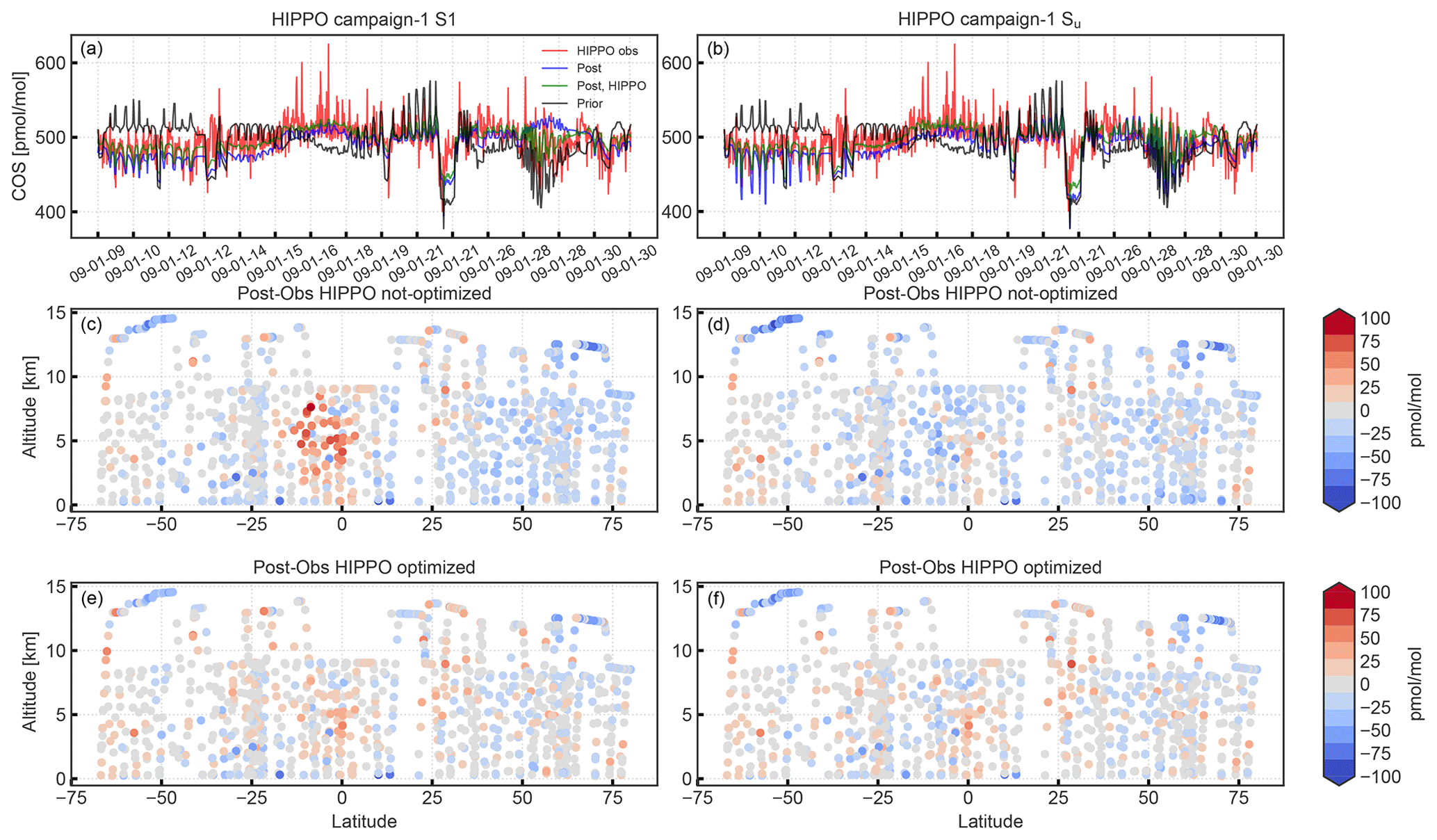
Figure 8 HIPPO campaign-1 COS observations compared to results from inversions S1 (a, c, e) and S_u (b, d, f). The first row shows time series of HIPPO observations (red), prior (black), posterior (blue), and posterior with HIPPO observations assimilated (green). The middle and bottom rows show the model minus observations in a latitude–height plot for inversions with and without assimilating HIPPO observations, respectively.

Although we currently cannot close the gap in the global COS budget with one specific known flux, it is instructive to explore the information content of a separate set of COS observations. In the next section, we will therefore evaluate the results of our inversions with HIPPO and NOAA airborne observations (Fig. 1).

3.3 Evaluation with HIPPO and NOAA airborne profiles

From Table 5 it is clear that for all inversions the comparison to HIPPO observations is not very favourable. Most notably, the simulations with optimized fluxes show strong negative biases and poor χ² statistics. However, Fig. 8 shows that the inversions S1 and S_u (blue lines) largely improve the correspondence to HIPPO campaign-1 observations (red), relative to the prior simulation (black). The posterior simulations capture the HIPPO observations much better. The remaining differences in the middle panels of Fig. 8 show the general underestimation of the model. However, inversion S1 overestimates HIPPO in the southern tropics, likely caused by too large flux adjustments over South America, the region sampled by HIPPO campaign 1.

Interestingly, when the HIPPO observations are additionally assimilated into the inversion, biases are largely removed (Fig. 8, lower panels) while the correspondence to the NOAA surface network deteriorates only slightly (Table 5). Posterior χ² values for the HIPPO campaigns remain relatively poor, however, signalling too strict error settings or processes that are not properly modelled.

From the comparison with HIPPO we find that our state vector has enough flexibility to fit additional observations and that the inversions are strongly observation-limited. Moreover, we find that the inversions based on only observations from the NOAA surface network tend to underestimate COS in the free troposphere. This is corroborated by observations from the NOAA airborne profiles, which are mostly collected over the USA (see Fig. 1). Figure 9 shows a comparison between profiles using results of inversion S1. Although most posterior profiles (blue) improve considerably compared to the prior simulation (black), they still underestimate observations (red) in the free troposphere. Note that the simulations based on inversion S1 correctly predict the drawdown of COS towards the surface for most measured profiles, and in particular the match with the LEF site is very good at the surface, which confirms the performance of the inversion. If HIPPO observations are additionally assimilated (green), the agreement in the free troposphere slightly improves. For S1, χ² for the profile comparison reduces from 27.7 to 20.1 and the bias reduces from −13.9 to −9.7 pmol mol⁻¹ (Table 5). This confirms the low bias of the free troposphere COS mole fractions in simulations with fluxes that are optimized using both NOAA surface and HIPPO observations.

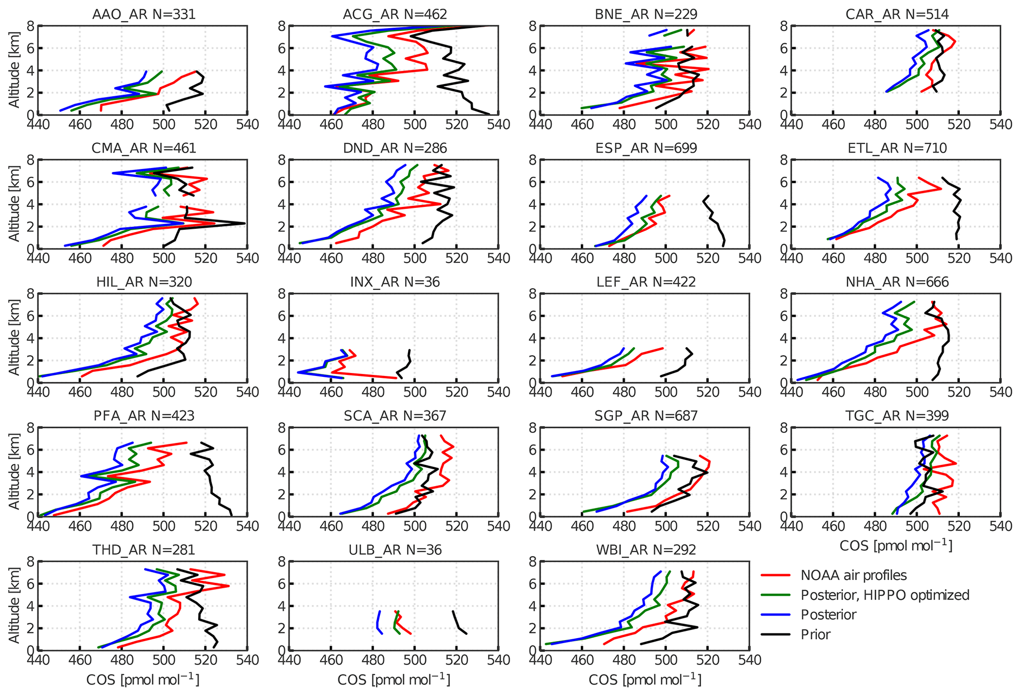
Figure 9 Prior (black) and posterior (blue) profiles of inversion S1, compared to NOAA aircraft profiles (red). Location (see Fig. 1) and number of observations are mentioned in the caption. The green lines are results from an inversion into which, besides NOAA surface observations, HIPPO observations are also assimilated. Note that the profiles are from all seasons.

It is now clear that inversions using surface data from the available NOAA network sites will not be able to separate various source categories and specifically not in the data-void tropics. In the next section we will therefore investigate the prospects of using satellite data to constrain fluxes.

3.4 Satellite validation

In Fig. 10 we present a comparison between MIPAS, ACE-FTS and co-sampled TM5 COS profiles. The latitude–height distributions of MIPAS, TM5 (convolved with the MIPAS AK) and ACE-FTS are shown in Fig. 10a–c. In Fig. 10d we show averaged ACE-FTS, MIPAS and TM5 profiles, the latter two resulting from collocations with respect to ACE-FTS. The TM5 profiles shown are from the prior simulation (black), from inversion S1 (blue) and from inversion S1 with additional assimilation of HIPPO profiles (green). They are all convolved with the MIPAS AK.

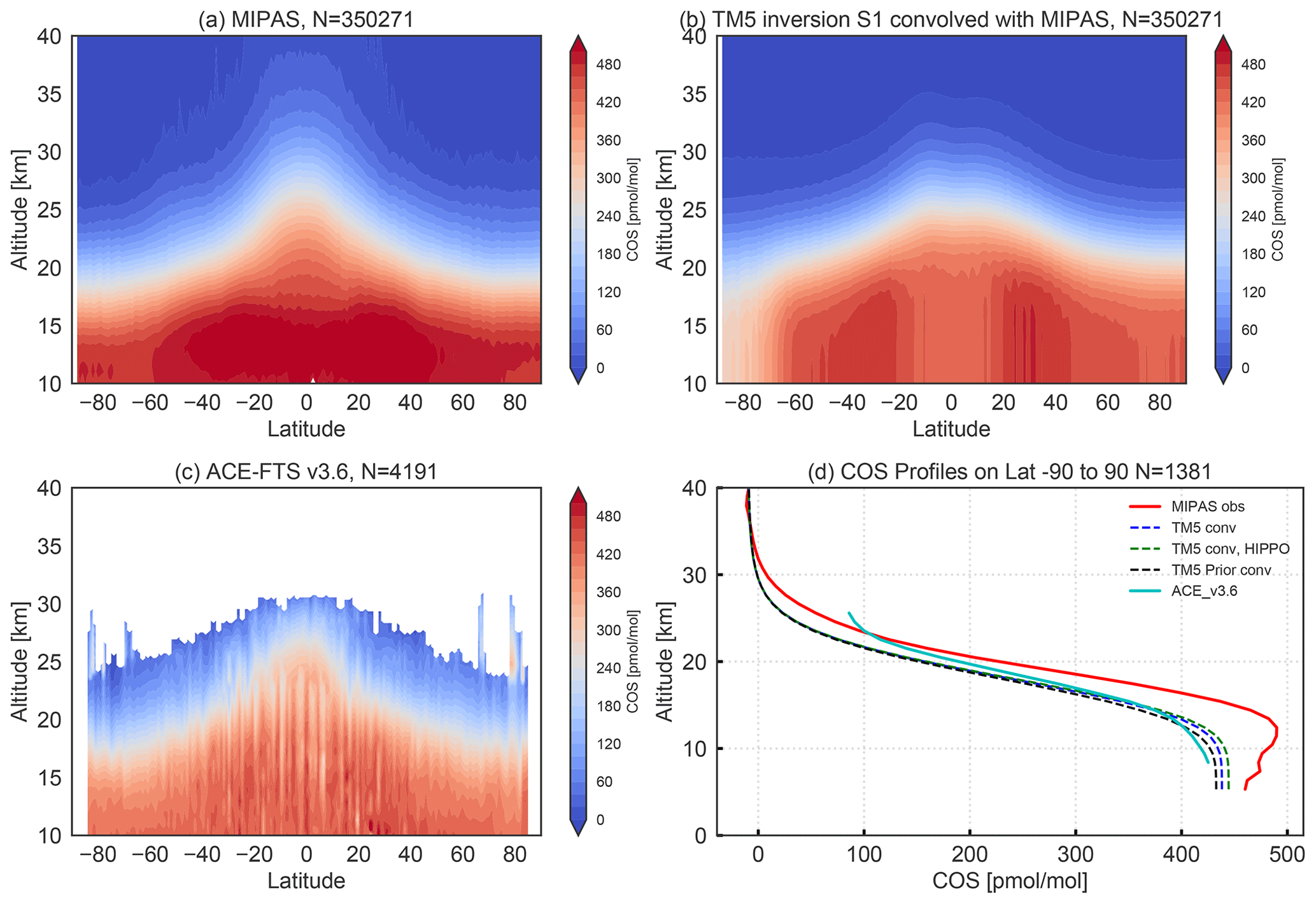
Figure 10 Comparison of MIPAS and ACE-FTS v3.6 with TM5 results from inversions for 2009. (a) Latitude–height contour plot of MIPAS; (b) TM5 S1 convolved with the MIPAS AK; (c) ACE-FTS profiles; (d) average of collocated profiles for MIPAS (red), TM5 convolved with MIPAS AK from inversion S1 (blue), TM5 convolved from inversion S1 (with HIPPO observations assimilated) (green), TM5 convolved prior (black) and ACE-FTS. In (d) TM5 and MIPAS profiles are collocated with respect to ACE-FTS profiles within a temporal offset of 6 h and a spatial distance of 5^∘. The number of collocated profiles is 1381.

In general, TM5 reproduces the observed pattern of COS well but with lower values in the tropical upwelling region at around a 25 km altitude. The comparison between ACE-FTS and MIPAS is consistent with findings of Glatthor et al. (2017), who found that ACE-FTS is systematically lower in the UTLS region. Moreover, they found that MIPAS data showed no bias compared to MkIV and SPIRALE COS balloon profiles, which also exhibit higher COS values than ACE-FTS (Krysztofiak et al., 2015; Velazco et al., 2011). TM5 profiles, after convolution with the MIPAS AK, are in between MIPAS and ACE-FTS. Compared to the other TM5 runs, prior TM5 profiles (black) show the lowest values around the tropopause. Again, TM5 profiles optimized by HIPPO and NOAA observations (dashed green line in Fig. 10d) show a slight increase in the upper troposphere compared to the optimization with only NOAA surface-site data (dashed blue line).

To compare the different inversions with respect to the simulated latitude–longitude distribution, Fig. 11 shows a comparison of COS between TM5 inversions and MIPAS at 250 hPa in June to August. Similar results at 250 hPa from September to November and at 150 hPa from June to August are shown in the Supplement (Figs. S8 and S9). MIPAS COS represents a 2002–2011 average taken from Glatthor et al. (2017). TM5 results have been averaged over 2008–2010. The distributions of COS in all inversions match relatively well with MIPAS. Note, however, that we adjusted the TM5 results by +25 pmol mol⁻¹ to match the colour scale of MIPAS. The COS distribution from the prior simulation correctly simulates low COS over the Amazon and Africa but is clearly too high over northern latitudes. This latter aspect is partly solved by the inversions. If we concentrate on the observed COS minimum over the Atlantic, Africa and the Amazon, inversions S1 and S3 shift this minimum to the east, consistent with the COS biosphere flux increment shown in Fig. 7 for S1. Inversions S_u and S2 exhibit a better comparison with MIPAS, suggesting that the large increments of the tropical biosphere over South America (Fig. 7) are unrealistic. However, assigning the missing tropical source totally to ocean emissions (S2) appears to overestimate the COS drawdown over the Amazon.

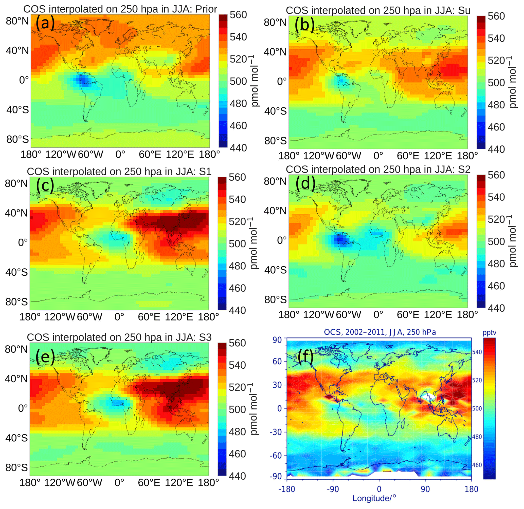
Figure 11 COS mole fraction comparison of MIPAS and TM5 inversions at 250 hPa in June to August. (a–e) TM5 prior and inversions S_u, S1, S2 and S3, respectively. (f) Captured from Fig. 11 in Glatthor et al. (2017). TM5 results represent a 2008–2010 average, and MIPAS is averaged over 2002–2011. Because TM5 results are systematically lower than MIPAS, 25 pmol mol⁻¹ is added to the TM5 results for a better visual comparison.

TM5 results are also compared to the nadir-viewing TES instrument. To this end, COS columns of TM5 (convolved with the TES AK; see Eq. 1) and TES are averaged in 20 latitudinal bins between 32^∘ S and 32^∘ N. Outside this latitude band, TES observations become too noisy for a reasonable comparison. Comparisons are shown for the months March, June, September and December in Fig. 12, based on inversion S1 and averaged over the years 2008–2011. We applied an arbitrary bias correction of β=1 in Eq. (1) to obtain a reasonable fit to TES observations. After assimilation, the agreement with TES improves compared to the prior, but the latitudinal gradients remain generally smaller in the model. The inversion into which the HIPPO observations are also assimilated increases the simulated mole fractions, confirming our findings based on the airborne observation. In general, the TES-derived columns offer a good perspective to better constrain the COS budget in the tropics. Due to the sensitivity of TES to COS in the middle troposphere (Kuai et al., 2015), the assimilation of TES into our 4DVAR system might be able to differentiate between the biosphere and ocean signal, something that turned out to be difficult using NOAA surface observations only.

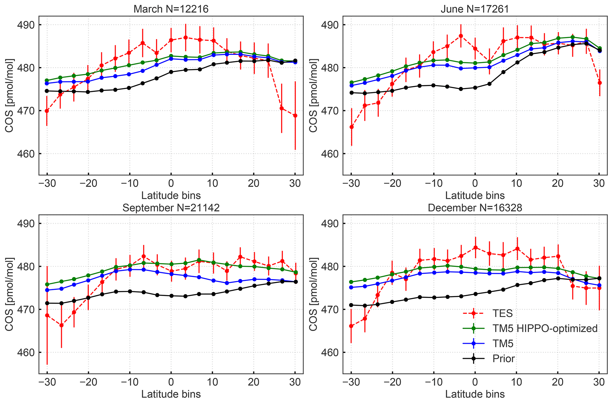
Figure 12 Column-averaged COS mole fractions sampled by TES (red), model prior (black), model posterior (blue) and posterior with HIPPO observations assimilated (green) for March, June, September and December. The columns are averaged over 2008–2010 in 20 latitudinal bins from 32^∘ S to 32^∘ N. The result of inversion S1 is shown. Error bars on TES represent variability in the measurements, and the number of observations is given in the caption. Variability is mostly determined by measurement noise. A bias correction of β=0.1 was applied when applying the TES AK in Eq. (1).

3.5 Discussion

In this study we have presented inversions focused on the closure of the global COS budget. In general, our inversion modelling framework based on the TM5-4DVAR system is well capable of closing the gap in the global budget (e.g. inversion S_u, S1 and S3) and of optimizing flux fields such that surface observations are well reproduced. However, due to the lack of observations, we are unable to unambiguously assign the missing COS sources to either missing ocean emissions or reduced tropical uptake by the biosphere. Firstly, the total number of observations remains relatively small, which leads to an under-determined inversion problem. Secondly, there are no observational sites that sample air masses from tropical Africa, South America and southeastern Asia, which are regions with important COS fluxes. An important next step will therefore be the utilization of satellite data in future inverse modelling studies. In the current study, we did not include all exchange fluxes that are reported in the literature (Whelan et al., 2018). In general, we find that our inversions still underestimate COS in the free troposphere. Here, there might be a role for volcanic emissions (25–42 Gg a⁻¹; Whelan et al., 2018), or “unnoticed” tropical sources like wetland exchange (−150 to 290 Gg a⁻¹; Whelan et al., 2018). Volcanic emissions are important to mitigate the stratospheric aerosol loading in the stratosphere (Sheng et al., 2015) and might be able to reduce the gap between modelled COS by TM5 and measurements. Alternatively, missing COS could come from an atmospheric oxidation process that converts CS₂ or DMS to COS. We did not find strong evidence for enhanced CS₂ emissions from tropical oceans in our S1 inversion, although inversion S2 produced reasonable COS simulations by optimizing only COS and CS₂ emissions from the ocean. Moreover, our “best” S_u inversion produced a flux field that indicated enhanced tropical sources over both land and ocean (Fig. 5). Thus, field studies that address tropical COS exchange processes are urgently needed (Lennartz et al., 2020).

We have also considered some variations in our modelling setup. A unique approach of our study is the inclusion of CS₂ and DMS as COS precursors. We tested the effect of emitting CS₂ ocean and anthropogenic sources directly as COS in an additional forward model simulation. As shown in Fig. S10, COS mole fractions would become significantly larger close to CS₂ emission hot spots in Asia, Europe and the USA. At selected stations (LEF in the USA and MHD in Europe, Fig. S10a and b), we observe COS mole fractions that are up to 40 pmol mol⁻¹ higher during events where emitted CS₂ is advected to the station. Some ambiguity has been introduced about the CS₂ lifetime (Khan et al., 2017). In our S_u inversion, the lifetime of CS₂ is estimated as 9.4 d (CS₂ burden divided by CS₂ loss by OH), substantially longer than the ∼3 d lifetime mentioned in Khan et al. (2017). Future work should be based on the rate recommendations in Sander et al. (2006). Thus, we conclude that inclusion of CS₂ as a separate tracer is important if we want to understand emissions of CS₂ and COS, which have distinctly different spatial patterns (e.g. see Fig. S4). Regarding DMS as a COS precursor, we have evaluated its importance by performing a NO–DMS inversion, in which DMS as a tracer was removed and the 162 Gg a⁻¹ DMS source was added to the COS “unknown flux” in inversion S_u. In Fig. S11, it can be seen that the NO–DMS inversion shows larger adjustment over both oceans and continents but that the pattern remains comparable to inversion S_u.

The use of COS as a proxy for gross primary productivity on a global scale needs a better level of understanding of the biosphere flux. Here we used monthly prior flux fields calculated with SiB4 (Berry et al., 2013) in which soil exchange and vegetation uptake are combined. In future studies, we might need a better prior description of this important global COS sink. For instance, recent studies (Ogée et al., 2016; Sun et al., 2018; Meredith et al., 2019; Spielmann et al., 2020) stress the importance of the soil–atmosphere COS exchange. Our inversions S1 and S3 calculate large increments in the biosphere exchange (Fig. 7), with generally less uptake in the tropics (turning the flux even into a COS source) and enhanced uptake in the NH high latitudes. Quantitatively, the COS uptake is reduced from a prior value of 1053 to 557 Gg a⁻¹ to close the gap in the COS budget. While we seriously question the validity of this result given the fact that most flux adjustments are projected in the data-void tropics, it is still instructive to consider the feedback of the atmospheric COS mole fractions on COS uptake. Since biosphere models operate mostly uncoupled to atmospheric transport models, we used a fixed mole fraction of 500 pmol mol⁻¹ to construct the prior biosphere fluxes. However, observations clearly show a large drawdown of COS near the surface (Campbell et al., 2008; Hilton et al., 2017; Spielmann et al., 2020; Berkelhammer et al., 2020). We therefore explored the calculations in SiB4 and found that biosphere flux should scale linearly with atmospheric COS mole fractions (Berry et al., 2013). To estimate the potential impact of reduced mole fractions at the surface on the biosphere flux, we corrected the monthly SiB4 fluxes as

$$\begin{array}{}\text{(11)}& f_{\mathrm{biosp},\mathrm{cor}}=f_{\mathrm{biosp}}{\displaystyle \frac{y\left(\mathrm{COS}\right)}{\text{500}\text{pmol}{\text{mol}}^{-\mathrm{1}}}},\end{array}$$

where f_biosp and f_biosp, cor are the original and corrected monthly biosphere fluxes on the TM5 grid and y(COS) is the monthly mean COS mole fractions (pmol mol⁻¹) in the first model layer (approximately 50 m) from inversion S_u. This simple correction, based on monthly mean fields, changes the biosphere sink from 1053 to 851 Gg a⁻¹, an update of 202 Gg a⁻¹ (Figs. S12, S13 and S14) and closer to the 738 Gg a⁻¹ reported by Berry et al. (2013). Interestingly, the corrected flux is strongly reduced over regions with an active tropical biosphere, in line with results from inversions S1 and S3. This indicates that uptake of COS should be treated as a first-order loss process and that the SiB4 prior fields based on fixed atmospheric mole fractions of 500 pmol mol⁻¹ likely overestimate COS uptake. However, such an approach makes the optimization problem non-linear. This, as well as the challenge of assimilating satellite observations, will be the subject of future studies.

4 Conclusions

In this study, we have implemented an inverse modelling framework for COS, coupled to the budgets of CS₂ and DMS. Inversions using the NOAA surface observation network have been evaluated with observations from HIPPO, airborne observations and satellite products. Conclusions are as follows:

• In line with earlier studies, our inversions point to missing sources in the tropics and missing sinks at high latitudes. With seasonal decomposition of the optimized unknown COS flux, it is found that the missing sources show regional seasonality, indicating regional source or sink impacts. Whether the missing sources in the tropics originate from the land or ocean cannot be determined currently because of a lack of observations in the tropics.

• Simulations that are optimized by only NOAA surface observations from 14 sites lack information about COS in the free troposphere. When the short-term HIPPO aircraft sampling programme is used as an additional data source in the inversions, the comparison to NOAA airborne observations and satellite products generally improves.

• Comparison between TM5 inversions and satellite data shows that COS in the model is systematically lower than MIPAS, and inversions reproduced the tropospheric COS spatial distribution well, specifically for inversions S_u and S2. These comparisons indicate that the missing tropical source likely originates from a combination of underestimated ocean emissions and overestimated biosphere uptake. Part of the tropical sources can be explained by the dependence of COS uptake on atmospheric mole fractions.

• Future improvements are expected from the assimilation of satellite data and better prior descriptions of the ocean and biosphere fluxes.

Our future plan is therefore to assimilate satellite data into our 4DVAR inverse modelling system to have better constraints on COS in the free troposphere and lower stratosphere. Other developments target the coupling of COS and CO₂ in a shared inverse modelling system, with the aim of better constraining gross primary productivity.