A satellite-data-driven framework to rapidly quantify air-basin-scale NO_x emissions and its application to the Po Valley during the COVID-19 pandemic

The evolving nature of the COVID-19 pandemic necessitates timely estimates of the resultant perturbations to anthropogenic emissions. Here we present a novel framework based on the relationships between observed column abundance and wind speed to rapidly estimate the air-basin-scale NO_x emission rate and apply it at the Po Valley in Italy using OMI and TROPOMI NO₂ tropospheric column observations. The NO_x chemical lifetime is retrieved together with the emission rate and found to be 15–20 h in winter and 5–6 h in summer. A statistical model is trained using the estimated emission rates before the pandemic to predict the trajectory without COVID-19. Compared with this business-as-usual trajectory, the real emission rates show three distinctive drops in March 2020 (−42 %), November 2020 (−38 %), and March 2021 (−39 %) that correspond to tightened COVID-19 control measures. The temporal variation of pandemic-induced NO_x emission changes qualitatively agrees with Google and Apple mobility indicators. The overall net NO_x emission reduction in 2020 due to the COVID-19 pandemic is estimated to be 22 %.

1 Introduction

Satellites have revolutionized our ability to observe the Earth's atmospheric composition and air quality. Vertical column densities (VCDs) of reactive species such as NO₂, HCHO, SO₂, and NH₃ are retrieved from the observed radiances in the ultraviolet, visible, or infrared bands. The tropospheric VCD (TVCD) retrieval of NO₂ has been widely used to infer the emissions of nitrogen oxides (NO_x = NO₂ + NO), which is at the center stage of atmospheric chemistry by modulating ozone and secondary aerosol formation (Kroll et al., 2020). The NO_x emissions are dominated by anthropogenic fossil fuel combustion, and its chemical lifetime in the lower troposphere is relatively short. Consequently, the satellite-observed NO₂ TVCD is highly responsive to perturbations of human activities, including economic recession (Castellanos and Boersma, 2012; Russell et al., 2012), long- and short-term emission regulations (Duncan et al., 2016; Mijling et al., 2009; Witte et al., 2009), and the ongoing global pandemic caused by the coronavirus, or COVID-19 (Bauwens et al., 2020; Liu et al., 2020; Huang and Sun, 2020).

Although NO₂ TVCD is well established as an indicator of NO_x emission, the quantitative connection between NO₂ abundance and NO_x emission is confounded by nonlinear chemistry and meteorology (Valin et al., 2014; Goldberg et al., 2020; Keller et al., 2021). Many NO_x emission inference methods have been proposed using chemical transport models (CTMs) that resolve chemistry and meteorology in space and time, including mass balance (Martin et al., 2003; Lamsal et al., 2011; Zheng et al., 2020), four-dimensional variational data assimilation  (4D-Var,  Qu et al., 2019; Wang et al., 2020), and Kalman filters (Miyazaki et al., 2020a; Mijling and Van Der A, 2012; Ding et al., 2020). Ding et al. (2020) and Miyazaki et al. (2020b) used CTMs to estimate NO_x emission reduction in China in the early phase of the COVID-19 pandemic, but it is a growing challenge to match the resolution, lag time, and running cost of CTMs with the new generation of satellite products that resolve the NO₂ spatial distribution down to a few kilometers. As such, observational-data-driven approaches have also been developed, which attempt to derive emissions based on the observed column abundance and without invoking CTMs. A common way to estimate emissions of short-lived species like NO_x is to retrieve emission and lifetime simultaneously by fitting an exponentially modified Gaussian (EMG) function to the downwind plumes from relatively isolated emission sources (e.g., cities or power plants) (Beirle et al., 2011; Liu et al., 2016; de Foy et al., 2015; Lu et al., 2015; Goldberg et al., 2019a, b; Laughner and Cohen, 2019; Valin et al., 2013; Zhang et al., 2019). However, the observational-data-driven approaches using OMI only provide warm-season or annually averaged emissions and hence cannot capture the rapidly varying and ongoing COVID-19-induced emission changes. The availability of much more finely resolved TROPOMI observations since 2018 enables observation-based NO_x emission estimates at daily scale over a megacity (Lorente et al., 2019).

Based on satellite observations and reanalysis wind speed, we develop a novel framework that directly and quickly quantifies air-basin-scale NO_x emissions at monthly resolution. We demonstrate this framework using NO₂ TVCDs from both OMI and TROPOMI over the Po Valley air basin in Italy, which has been severely affected by COVID-19 (Filippini et al., 2020). The COVID-19-induced emission decline has to be disentangled from pre-existing trends and seasonality. Leveraging the long data record from OMI, we build a statistical model using historic emission rates and predict the business-as-usual trajectory in 2020–2021. The difference between this trajectory and the real 2020–2021 emissions reflects the net effect of COVID-19. As the pandemic and the controlling policies are still evolving in 2021, this extrapolation using a long-term satellite record offers a significant advantage over a simple 2020 vs. 2019 comparison. Although only NO_x emission in the Po Valley is investigated in this work, this satellite-data-driven framework can be readily applied to other satellite products and regions to rapidly characterize emission changes.

2 Materials

2.1 Satellite TVCDs

We use the most recent (version 4) NO₂ level 2 TVCD retrievals from the NASA operational standard product for OMI (Lamsal et al., 2021). The operational TROPOMI NO₂ product (van Geffen et al., 2020; ESA, 2018) used in this study underwent several algorithm updates since its public release in 30 April 2018. A significant cloud retrieval algorithm update happened in November 2020, leading to substantial increase in retrieved NO₂ TVCD in polluted regions. The TROPOMI NO₂ algorithm is expected to be updated with full reprocessing in 2021 to improve its consistency and continuity (GES DISC, 2021). The level 2 orbits covering the geographical region of interest over every month are standardized into single files from October 2004 to June 2021 for OMI and from May 2018 to June 2021 for TROPOMI. We only use quality-assured level 2 pixels with cloud fraction <0.3 and solar zenith angle $<\mathrm{70}{}^{\circ }$. Throughout the OMI mission, its across-track pixels are limited to 5–23 out of 1–60 to avoid the row anomaly and keep the time series analysis consistent (Duncan et al., 2016; Schenkeveld et al., 2017). TROPOMI features 450 pixels across its 2600 km swath and a nadir pixel size of 3.5×5.5 km² (3.5×7 km² before 6 August 2019), leading to significantly higher spatial resolution than OMI, whose nadir pixel size is 13×24 km².

Validation studies of both OMI and TROPOMI NO₂ TVCDs consistently show systematic low biases (Choi et al., 2020; Judd et al., 2020; Verhoelst et al., 2021), which can be attributed to the horizontally coarse a priori profile representation as well as uncertainties in surface albedo and cloud parameters in the air mass factor (AMF) calculation. This low bias matters less for emission trend analysis but will proportionally impact the absolute values of the derived emission rate. This study focuses on an air basin in which a high level of pollution is confined, and the spatial gradient is significantly less than many other polluted regions. The relative biases between OMI and TROPOMI NO₂ TVCD are assessed by comparing strictly collocated level 2 retrievals and given in Appendix A. The OMI NO₂ TVCD is generally higher than TROPOMI in the cold season, with a monthly OMI–TROPOMI normalized mean bias (NMB) up to over 30 %, whereas the TROPOMI TVCD is generally higher in the warm season, with a monthly OMI–TROPOMI NMB down to −20 %.

2.2 Study domain and NO_x emission inventories

The Po Valley air basin is delineated according to the boundary between the flat terrain in northern Italy and mountain ranges in the north, west, and south as well as the Adriatic Sea coastline in the east, as shown in Fig. 1. The air basin area is 6.6×10⁴ km². The west–east length scale is ∼500 km, and the south–north length scale is ∼300 km; both are larger than the square root of basin area (257 km) due to the irregularity of the basin shape. We contrast our derived monthly air-basin-scale NO_x emission rates with four global inventories. Their emission distributions near the Po Valley air basin are illustrated in Fig. 1. The Jet Propulsion Laboratory (JPL) chemical reanalysis provides monthly top-down emission estimates at $\mathrm{1.1}{}^{\circ }\times \mathrm{1.1}{}^{\circ }$ spatial resolution for 2005–2019 (Miyazaki et al., 2019, 2020a). The NO_x emissions from the JPL chemical reanalysis (Fig. 1a) are constrained by assimilating O₃, NO₂, CO, HNO₃, and SO₂ from the OMI, GOME-2, SCIAMACHY, MLS, TES, and MOPITT satellite instruments (Miyazaki et al., 2020a) and are considered to have the highest accuracy in spite of the relatively low spatial resolution. The other three are bottom-up emission inventories, including the Community Emission Data System (CEDS;  McDuffie et al., 2020), the Emissions Database for Global Atmospheric Research version 4.3.2 (EDGAR;  Crippa et al., 2018), and the Peking University NO_x inventory (PKUNOx;  Huang et al., 2017). The CEDS inventory is spatially resolved at $\mathrm{0.5}{}^{\circ }\times \mathrm{0.5}{}^{\circ }$ (Fig. 1b) and available monthly from 1970 to 2017. Both EDGAR and PKUNOx are at $\mathrm{0.1}{}^{\circ }\times \mathrm{0.1}{}^{\circ }$ spatial resolution (Fig. 1c, d). EDGAR is available annually from 1970 to 2012, and PKUNOx is available monthly from 1960 to 2014. Because of the large grid sizes of the JPL chemical reanalysis and CEDS inventory, we calculate the air-basin-mean emission rate by averaging inventory grid cells that overlap with the Po Valley air basin, weighted by the overlapping area.

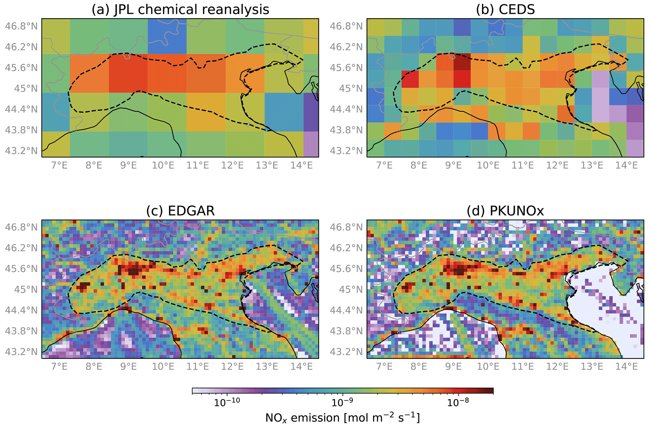
Figure 1 Spatial distribution of annual NO_x emissions in 2005 near the Po Valley air basin (black dashed line) from (a) JPL chemical reanalysis, (b) CEDS, (c) EDGAR, and (d) PKUNOx.

2.3 Wind fields

We use wind fields gridded at $\mathrm{0.25}{}^{\circ }\times \mathrm{0.25}{}^{\circ }$ spatial resolution and hourly temporal resolution from the ERA5 reanalysis meteorology (Hersbach et al., 2020). The relevant ERA5 fields are spatiotemporally interpolated at each individual OMI and TROPOMI level 2 observation. Previous observational-data-driven emission inference studies represented horizontal advection of NO₂ (or similar short-lived tracers like SO₂ and NH₃) by 10 m wind above the surface (de Foy et al., 2015), 100 m above the surface (Goldberg et al., 2020), vertically averaged wind from the surface to 500 m (Lu et al., 2015; Liu et al., 2016; Goldberg et al., 2019a), or vertically averaged wind from the surface to 1000 m (Fioletov et al., 2017; Dammers et al., 2019). Figure 2 quantitatively compares the wind speeds of these four options using ERA5 data sampled at OMI level 2 observations within the Po Valley air basin boundary (see Fig. 1) from October 2004 to February 2021. These four wind speeds show strong linear correlation, with stronger winds when higher altitudes are involved. The surface–1000 m wind speed is almost twice as strong as the 10 m wind, whereas the two intermediate options, the 100 m wind and the surface–500 m wind, are similar with a difference of 13 %. The wind directions among those four options show much larger discrepancy, but only the wind speeds will be used in this study.

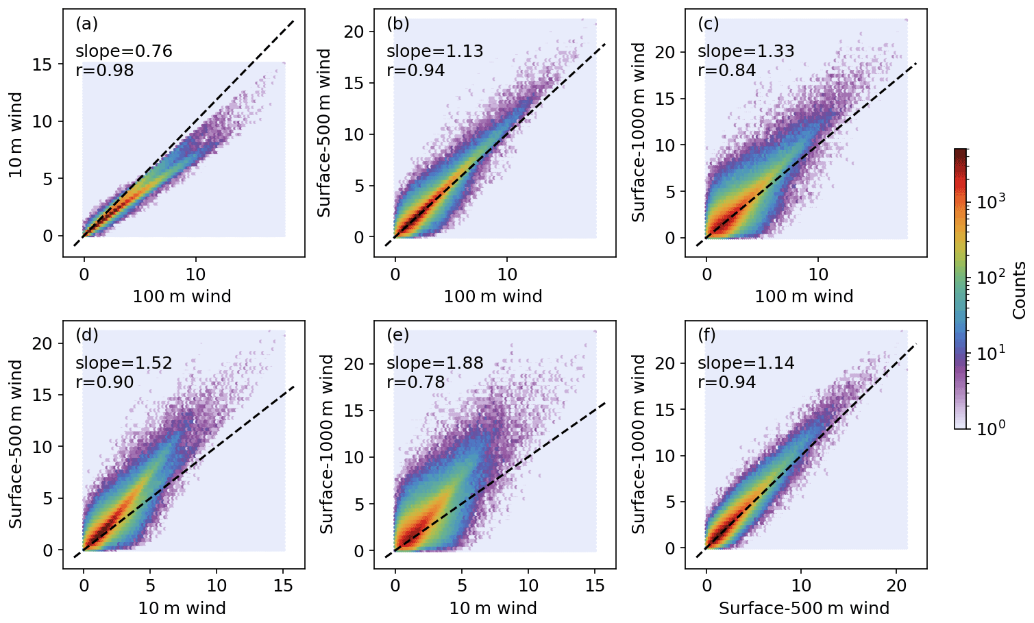
Figure 2 Correlations between speeds of 100 m wind and 10 m wind (a), 100 m wind and surface–500 m wind (b), 100 m wind and surface–1000 m wind (c), 10 m wind and surface–500 m wind (d), 10 m wind and surface–1000 m wind (e), and surface–500 m wind and surface–1000 m wind (f). Wind data are from ERA5 meteorology sampled at valid OMI NO₂ observation locations in the Po Valley air basin in 2004–2021. The slopes labeled in the plot are from orthogonal regression, and r is the correlation coefficient (wind speed unit: m s⁻¹).

2.4 In situ NO_x observations

We use the ground-based NO_x observations over the Po Valley available from the air quality data portal of the European Environment Agency (EEA) to constrain the temporal variation of the NO_x : NO₂ ratio (EEA, 2021). The validated data (E1a) are used for the years 2013–2019 and combined with up-to-date data (E2a) for 2020–2021. Only valid hourly data labeled at 13:00 and 14:00 local time with both NO₂ and NO_x available are included in the analysis. We include only ground-based observations within OMI level 2 pixels with cloud fraction <0.3, but the resultant all-sky vs. clear-sky differences are insignificant.

3 Methods

3.1 Construction of column–wind speed relationships by physical oversampling

A key step to estimating NO_x emissions from the observed NO₂ TVCDs is to construct the column–wind speed relationship by averaging column amounts over a range of wind speed intervals. Physical oversampling (Sun et al., 2018) provides a flexible way to spatiotemporally average satellite data with proper weighting and slice the data under different environmental conditions (e.g., wind speed). The averaged NO₂ TVCD (〈Ω〉) given sets of filtering criteria with respect to space (s), time (t), and other level 2 parameters (p) can be calculated as

$$\begin{array}{}\text{(1)}& \langle \mathrm{\Omega }\rangle (s,t,p)={\displaystyle \frac{{\sum }_{j\in s}{\sum }_{i\in t,p}{w}_{i,j}{\mathrm{\Omega }}_i}{{\sum }_{j\in s}{\sum }_{i\in t,p}{w}_{i,j}}}.\end{array}$$

Here j is the index of each level 3 grid cell at 0.01^∘ resolution, and j∈s includes all grid cells satisfying the spatial aggregation criterion s (e.g., within the boundary of an air basin). Ω_i is NO₂ TVCD retrieved at level 2 pixel i. i∈t and p keep only level 2 pixels satisfying time filtering criteria (e.g., within a calendar month) and parameter filtering criteria (e.g., wind speed at the level 2 pixel within a certain interval). w_i, j is the weight of level 2 pixel i at level 3 grid cell j and depends on the spatial response of pixel i at grid cell j as well as the retrieval uncertainty at pixel i (Zhu et al., 2017; Sun et al., 2018).

The column–wind speed relationship for an air basin over a certain time interval is an array of averaged NO₂ TVCDs over different wind speed intervals (every 0.5 m s⁻¹ in this study):

$$\begin{array}{}\text{(2)}& \begin{array}{rl}& \langle \mathbf{\Omega }\rangle =[\langle \mathrm{\Omega }\rangle (\mathrm{0}{\text{ m\hspace{0.17em}s}}^{-\mathrm{1}}\le W<\mathrm{0.5}{\text{ m\hspace{0.17em}s}}^{-\mathrm{1}}),\langle \mathrm{\Omega }\rangle (\mathrm{0.5}{\text{ m\hspace{0.17em}s}}^{-\mathrm{1}}\\ & \le W<\mathrm{1.0}{\text{ m\hspace{0.17em}s}}^{-\mathrm{1}}),\mathrm{\dots }],\end{array}\end{array}$$

where W is the horizontal wind speed that is interpolated at level 2 pixels and is representative of horizontal advection. The four wind speed options shown in Fig. 2 are tested in this study. Figure 3 shows the column–wind speed (100 m wind here) relationships for OMI and TROPOMI over the Po Valley in December 2018–November 2020 grouped into four seasons. TROPOMI provides 2–3 times more coverage than OMI, as indicated by the dot sizes, but ∼ 50 times more valid level 2 pixels due to much finer spatial resolution, as labeled in the legends.

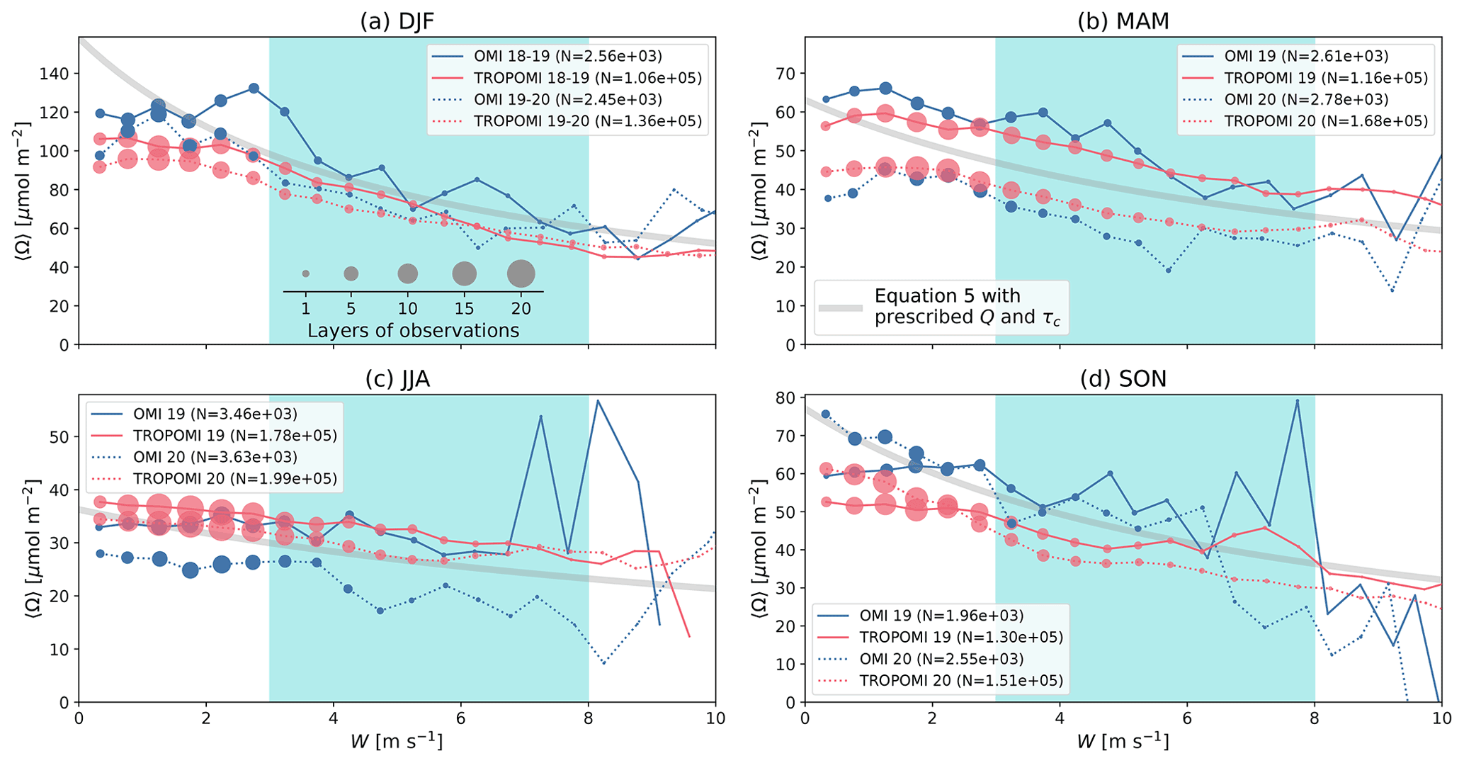
Figure 3 Relationships between OMI (blue) and TROPOMI (red) NO₂ TVCDs and wind speeds in December, January, February (DJF, a), March, April, May (MAM, b), June, July, August (JJA, c), September, October, and November (SON, d). Data are shown as solid lines for 2019 (including December 2018) and dotted lines for 2020 (including December 2019). Layers of level 2 observation coverage are indicated by dot sizes. N in the legends denotes the total number of level 2 pixels used in each column–wind speed relationship. Thick gray lines show the behaviors of Eq. (5) using prescribed NO_x emission rates (Q) of 240, 170, 160, and 170 µmol m⁻² and chemical lifetimes (τ_c) of 16, 9, 5.5, and 11 h for the four seasons. A modest wind range of 3–8 m s⁻¹ is highlighted by cyan shading.

3.2 Conceptual model of column–wind speed relationships

The emission rate over an air basin Q can be linked to the basin-average column amount through a box model:

$$\begin{array}{}\text{(3)}& \langle \mathbf{\Omega }\rangle ={\displaystyle \frac{Q}{\mathit{\varphi }A\left(\frac{\mathrm{1}}{{\mathit{\tau }}_{\mathrm{d}}}+\frac{\mathrm{1}}{{\mathit{\tau }}_{\mathrm{c}}}\right)}},\end{array}$$

where boldface symbols indicate vectors. The averaged NO₂ TVCD 〈Ω〉 and dynamic lifetime τ_d are both vectors resolved over a range of wind speeds W, ϕ is the NO_x : NO₂ ratio, A is the air basin area, and τ_c is the NO_x chemical lifetime. For cloud-free midday conditions in a polluted air mass, ϕ is conventionally assumed to be a constant of 1.32 with 20 % uncertainty in satellite-based NO_x emission estimates (Seinfeld and Pandis, 2006; Liu et al., 2016; Beirle et al., 2019). We further constrain the temporal variation of ϕ using observations in Sect. 4.3. The NO_x chemical lifetime may vary with wind speed depending on complicated nonlinear chemistry (Valin et al., 2013), so the scalar τ_c here should be considered the average value over the wind speed range. The high noise level in column–wind speed relationships prevents us from obtaining further wind speed dependence of the chemical lifetime. We simplify the dynamic lifetime dimensionally as the ratio between wind speed and the horizontal length scale of the air basin L:

$$\begin{array}{}\text{(4)}& {\mathit{\tau }}_{\mathrm{d}}={\displaystyle \frac{L}{\mathit{W}}}.\end{array}$$

This implicitly assumes that the horizontal wind efficiently ventilates pollution away from the air basin. However, the Po Valley is surrounded by mountains except the east side. Low wind conditions may only circulate air pollution within the basin boundary. We thus limit our analysis over moderate wind speeds as shown in Fig. 3. We do not find systematic differences in column–wind relationships over different wind directions over moderate wind speeds, so all wind directions are combined to maximize the number of observations. Then, the conceptual model of column–wind speed relationship can be written as

$$\begin{array}{}\text{(5)}& \langle \mathbf{\Omega }\rangle ={\displaystyle \frac{Q}{\mathit{\varphi }A\left(\frac{\mathit{W}}{L}+\frac{\mathrm{1}}{{\mathit{\tau }}_{\mathrm{c}}}\right)}}.\end{array}$$

Van Damme et al. (2018) and de Foy et al. (2015) have applied such box models to estimate short-lived NH₃ and NO_x emission rates by prescribing their chemical lifetimes. The dynamic lifetime was neglected (Van Damme et al., 2018) or calculated as the ratio between the near-surface wind speed and the half-edge length of the square box (de Foy et al., 2015). Similar box models have also been used to infer area-integrated CH₄ emission rates from column observations (Buchwitz et al., 2017; Varon et al., 2018). The chemical lifetime of CH₄ is negligible, and the dynamic lifetime was constrained by CTM simulations in these studies. Considering that the four wind options described in Sect. 2.3 (10 m, 100 m, surface–500 m, and surface–1000 m) give different yet strongly correlated wind speed values (Fig. 2), we expect that different L values are needed for those wind options. End-to-end emission rate estimates are performed using those four wind speed options with a range of L values in Sect. 4.1. We found that using 100 m wind and L=280 km for the Po Valley air basin (close to $\sqrt{A}=\mathrm{257}$ km) gives emission rate estimates that are most consistent with the JPL chemical reanalysis, which is considered to contain the smallest bias due to the high level of observational constraints. This is deemed a calibration for the dynamic lifetime and is specific to the Po Valley air basin.

The behavior of Eq. (5) is shown in Fig. 3 as gray lines with prescribed emission rate Q and chemical lifetime τ_c values for each season. Equation (5) implies that the column abundance should monotonously decrease with wind speed and, for the same chemical lifetime, scales with emission rate. When the chemical lifetime gets shorter, the $\mathrm{1}/{\mathit{\tau }}_{\mathrm{c}}$ term becomes larger relative to the dynamic lifetime term $\mathit{W}/L$, and hence the column abundance becomes a weaker function of wind speed. This is demonstrated by the fact that the NO₂ TVCDs decrease more rapidly with stronger wind in winter, indicating a longer NO_x chemical lifetime. The overall higher levels of NO₂ TVCDs in winter result from the combined effects of longer chemical lifetime and stronger emissions (see Sect. 4.4 for the seasonality of emission rates derived from this study as well as other top-down and bottom-up inventories).

As shown in Fig. 3, the observed column–wind speed relationship deviates from Eq. (5) at the lower and upper limits of wind speed. The simple parameterization of dynamic lifetime by $L/\mathit{W}$ assumes that the ventilation of the air basin is driven by horizontal advection, which is not valid when the basin air mass is stagnant. This is supported by the flattening of column–wind speed relationships at low wind speeds. At high wind speed, the number of valid observations rapidly decreases, leading to excessive noise. Therefore, we restrict our analysis to a moderate wind speed range of 3–8 m s⁻¹, as indicated by the shaded areas in cyan in Fig. 3.

3.3 Retrieving emission rate and chemical lifetime from column–wind speed relationships

As shown in Eq. (5), 〈Ω〉 and W are vectors with elements separated by wind speeds, so we may directly fit Eq. (5) to the observed column–wind speed relationships and simultaneously obtain emission rate Q and chemical lifetime τ_c. However, the information on τ_c mainly comes from the flatness of the observed column–wind speed relationship, and thus the fitted τ_c is highly sensitive to observational noise. Because Q and τ_c are strongly anticorrelated, the error in τ_c is efficiently propagated to the fitted Q. For example, the spikes in the observed OMI column–wind speed relationships in Fig. 3c and d would result in an unphysically low chemical lifetime and unrealistically high emission rate without proper regularization. To reliably retrieve Q for each calendar month throughout the OMI and TROPOMI record, we build a monthly climatology of τ_c from aggregated observation data and use it as prior information in a Bayesian optimal estimation framework (Rodgers, 2000; Brasseur and Jacob, 2017). The steps are summarized below, followed by a description in this section.

1. The monthly column–wind speed relationships are aggregated into 12 months for all the years (“climatological months” hereafter, in contrast to calendar months) separately for OMI (2004–2021) and TROPOMI (2018–2021). τ_c and Q are then fitted from the column–wind speed relationship of each climatological month.

2. The fitted τ_c values in the previous step are used as prior constraints in a Bayesian inversion to optimally estimate NO_x chemical lifetimes in the 12 climatological months.

3. The optimally estimated τ_c climatology is used as a prior constraint to retrieve emission rate Q and τ_c for each calendar month separately for OMI and TROPOMI.

3.3.1 Constructing and fitting climatological column–wind speed relationships

The column–wind speed relationship of each climatological month is averaged from 3-month windows in all available years. For example, the climatological month June is averaged from May–July in 2005–2020 for OMI and 2018–2020 for TROPOMI. Although each climatological column–wind speed relationship is averaged from a significant number of calendar months (48–51 for OMI and 7–9 for TROPOMI), unregularized nonlinear fitting of Q and τ_c is still highly unstable. Figure 4 shows the independent fitting of the column–wind speed relationships for each climatological month for OMI (panels a and b) and TROPOMI (panels c and d) as black symbols. The gray symbols show 100 bootstrap realizations for each climatological month, for which the calendar months used for averaging are selected randomly with replacement in each realization. This bootstrapping is necessary for realistic error estimation, as the fitting errors are substantially biased low due to strong anticorrelation of fitted parameters. Some climatological months (April, May, and September for OMI and August–October for TROPOMI) are characterized by a nonphysically high emission rate and low chemical lifetime, whereas others (January and February for OMI) are subject to a spuriously high chemical lifetime. Those originate from irregular features in the column–wind speed relationship (observable in Fig. 3) and tend to be more significant when satellite coverage is low. Because of the stochastic nature of atmospheric motion, those irregular features randomly appear in a limited number of calendar months, leading to wide spread of bootstrapping realizations and namely large uncertainties in emission rate and chemical lifetime estimates.

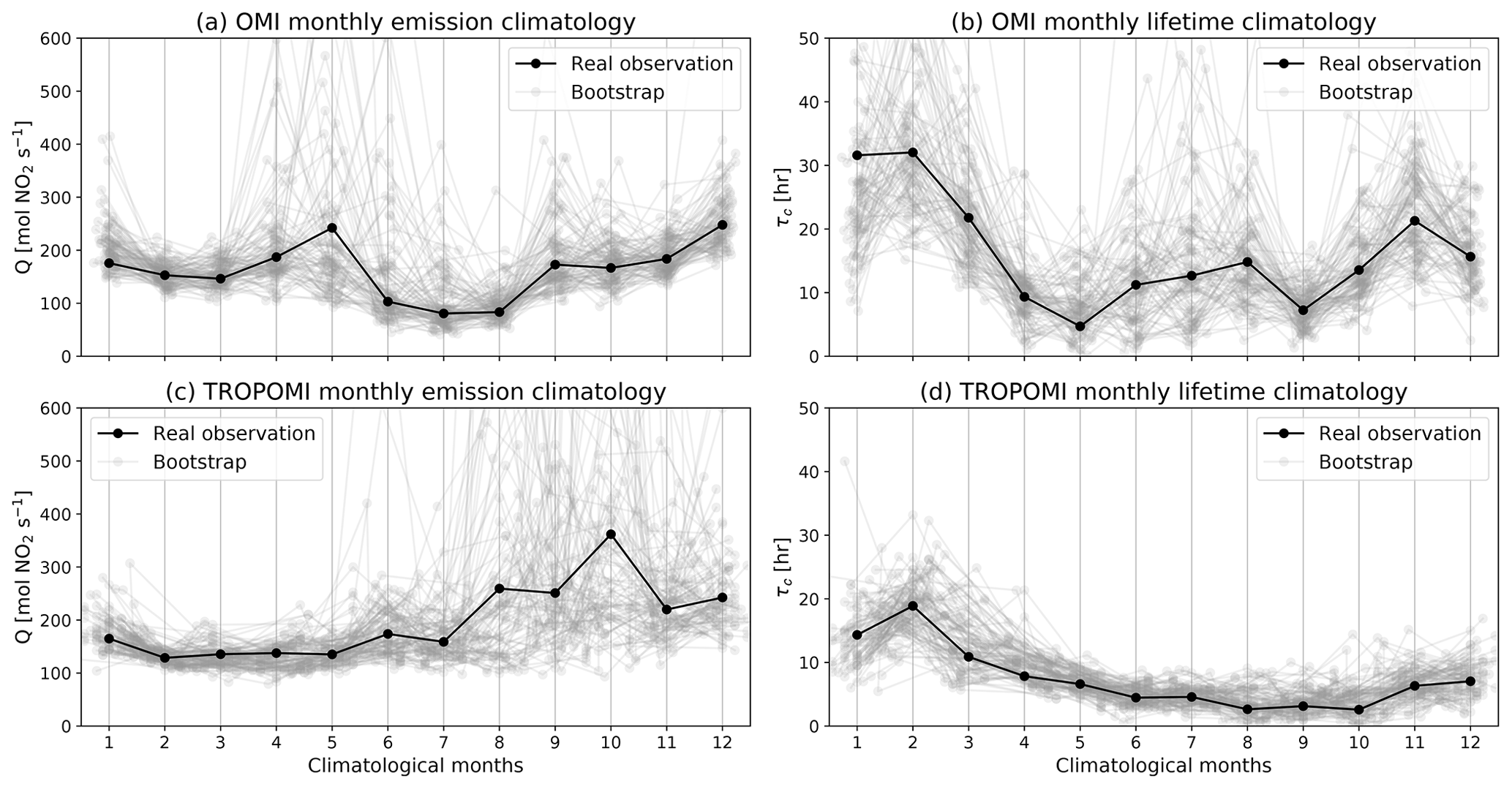
Figure 4 Fitting of the column–wind speed relationships for each climatological month for OMI (a, b) and TROPOMI (c, d). The black symbols are fitted from real observed data, and the gray symbols are bootstrapping realizations.

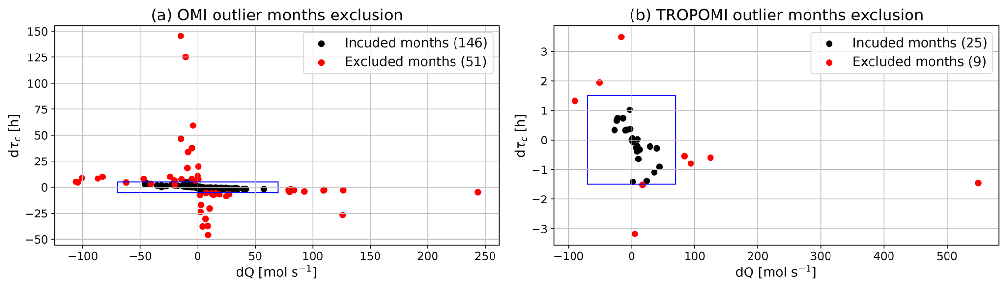
Figure 5 Exclusion of outlier months (red) for OMI (a) and TROPOMI. Each dot locates the differences of Q and τ_c from the corresponding climatological month fitting with and without a specific calendar month. The blue boxes show the boundaries delineating the maximum tolerated Q and τ_c influences from each calendar month to their corresponding climatological month.

We additionally remove “outlier” calendar months that would significantly alter the fitted τ_c and Q from the climatological column–wind speed relationship. These outlier months are often characterized by anomalously high NO₂ TVCDs over a few wind speed bins. For each calendar month, the corresponding climatological month is processed twice, with and without that calendar month included in the averaging. The differences of the fitted Q and τ_c the climatological month with and without a specific calendar month are displayed in Fig. 5. The calendar month is excluded as an outlier if the absolute value of its impact on the climatological Q is larger than 70 mol s⁻¹ or the absolute value of its impact on the climatological τ_c is larger than 1.5 h. The long record of OMI enables a second round of outlier removal, whereby the climatology is averaged from a single month (instead of 3-month window). It is impossible to do that for TROPOMI as 1 climatological month would only have 2–3 calendar months to average from. In this round, the max Q difference with and without including a calendar month is still 70 mol s⁻¹, but the max τ_c difference is relaxed to 5 h. The excluded calendar months are highlighted by red dots in Fig. 5. More winter months are excluded due to lower coverage and consequently noisier column–wind speed relationship. 53 % of winter calendar months in the OMI record are excluded, while the overall removal rate is 30 %.

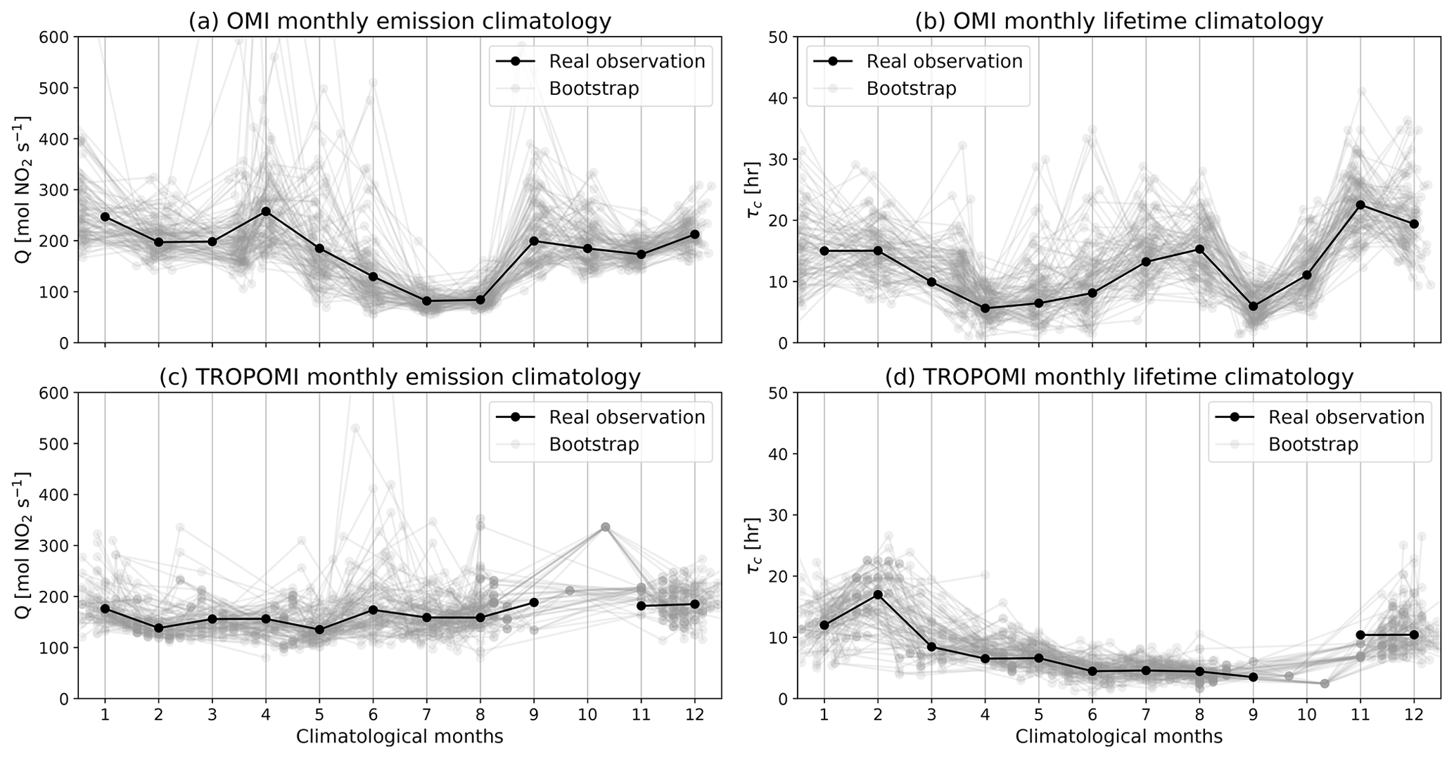
After identifying and excluding the outlier calendar months, the climatological column–wind speed relationships are finalized, and the climatology of emission rates and chemical lifetimes are fitted again. The results are shown in Fig. 6. The fitting quality is significantly improved, as indicated by the reduced variation of bootstrap realizations.

Figure 6 Similar to Fig. 4, but after outlier month exclusion shown in Fig. 5.

3.3.2 Optimal estimation of climatological chemical lifetime

The climatological NO_x chemical lifetimes fitted from the previous step are still unsatisfactory due to remaining large errors and correlation between fitted emission rates and chemical lifetimes. For instance, the OMI-based chemical lifetimes in climatological months April and September are unrealistically shorter than the summer months (Fig. 6b), which is inconsistent with the TROPOMI values (Fig. 6d) and corresponds to suspiciously high emission rates in those two climatological months (Fig. 6a). To further improve the climatology estimates, we incorporate the a priori information that the climatology should vary smoothly over the year through a Bayesian optimal estimation. The regularization from the optimal estimation will effectively suppress noise in the observed column–wind speed relationship.

In this optimal estimation setup, the 12 climatological column–wind relationships are concatenated into a single observation vector, and the 12 climatological chemical lifetimes and emission rates are retrieved simultaneously as a 24-element state vector. The fitted OMI- and TROPOMI-based τ_c values with outlier calendar months removed (black symbols in Fig. 6b and d) are averaged together and smoothed by a first-order Savizky–Golay filter with a 3-month window (Savitzky and Golay, 1964). This smoothed curve is used as the prior values of chemical lifetimes for both OMI and TROPOMI. The prior value for the emission rates is a constant 260 mol s⁻¹ for all climatological months. The prior error standard deviation is loosely set at 150 % for both Q and τ_c, and a time correlation scale of 1.5 months is assumed within the lifetime terms and the emission rate terms in the prior error covariance matrix. The model–observation mismatch error depends on satellite retrieval error, the representativeness of satellite observation in the air basin, and the chaotic nature of atmospheric motion. Little is known about the last two sources of error except that longer averaging time may reduce them, so we simplify the model–observation mismatch error as a single regularization factor λ that presents its overall variance. Optimal λ values are determined separately for OMI and TROPOMI by balancing the norm of fitting residuals and the norm of the prior error-weighted deviation of the solution to the prior using the L curve (Hansen and O’Leary, 1993). Details on the optimal estimation setup are provided in Appendix B.

Figure 7 Similar to Figs. 4 and 6, but using Bayesian optimal estimation incorporating the prior knowledge that the climatological emission rates and lifetimes should vary smoothly.

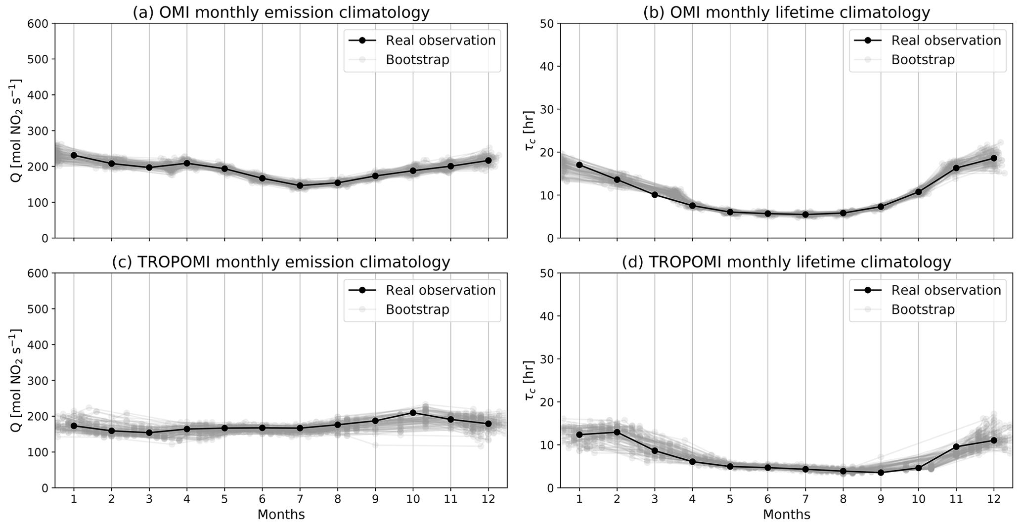
Figure 7 shows the posterior climatological emission rates Q (a and c) and chemical lifetimes τ_c (b and d) optimally estimated using OMI (a and b) and TROPOMI (c and d) column–wind speed relationships. After taking into account the correlations between climatological months via Bayesian optimal estimation, the errors are markedly reduced compared with individual climatological month fittings shown in Figs. 4 and 6. The climatological emission rates estimated from OMI data are higher than TROPOMI because overall the OMI record covers more early years (2004–2021) than TROPOMI (2018–2021), and the emission rate has been decreasing (see Sect. 4.4). The posterior climatological chemical lifetimes will be discussed in Sect. 4.2.

3.3.3 Optimal estimation of emission rates and chemical lifetimes for all calendar months

Finally, the monthly NO_x emission rate and chemical lifetime are retrieved from the column–wind speed relationships of all calendar months simultaneously in an optimal estimation algorithm (see Appendix B for technical details). The prior values of monthly τ_c are taken from the OMI-based τ_c climatology due to its overall higher quality and longer temporal coverage (see Fig. 7b and d and further discussion in Sect. 4.2). In other words, the OMI-based posterior chemical lifetimes in the 12 climatological months are used as the prior chemical lifetime in each calendar month for both OMI and TROPOMI. The prior error of calendar month τ_c is assumed to be 30 %, autocorrelated with an interannual timescale of 1.5 years and an intra-annual timescale of 1.5 months. This prior regularization to the τ_c terms is instrumental in the successful retrieval of the emission rate Q. The prior values of monthly Q are estimated from an exponential function fitted from the annually averaged JPL chemical reanalysis emission rates, and 100 % prior errors are used. No error correlations are assumed among the Q terms and between Q and τ_c terms. This configuration maximizes the information content of emission rates Q from observations while suppressing excessive noise in the results.

4 Results

4.1 Selection of air basin length scale

Equation (5) expresses the dynamic lifetime of NO_x in an air basin dimensionally as the ratio between a length scale L and wind speed. To assess the uncertainties induced by such simplification, we conduct sensitivity studies using end-to-end emission rate and chemical lifetime estimations described in Sect. 3.3 by switching wind speed options described in Sect. 2.3 and varying the prescribed values for L. The resultant OMI-based emission rates are compared with total surface NO_x emission rates from the JPL chemical reanalysis. We choose OMI-based emission rates due to long-term consistency and large overlap with the JPL chemical reanalysis. The combined wind speed option and L value that gives the closest agreement with the JPL chemical reanalysis monthly emission rate is selected, as the overall accuracy of the JPL chemical reanalysis is constrained by multiple observation datasets.

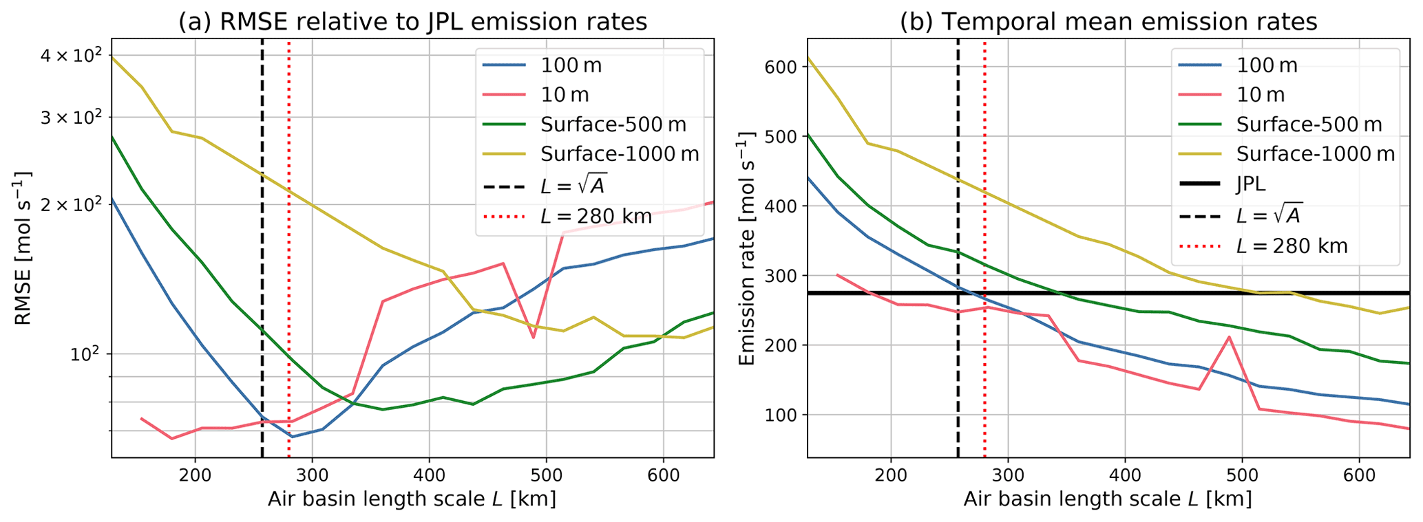
Figure 8 (a) Root mean square error (RMSE) of OMI-based emission rates relative to the monthly JPL chemical reanalysis emission rates for 2005–2019 when using 10, 100, surface–500 m, and surface–1000 m wind speeds as W in Eq. (5) and a range of L values. (b) Comparison of the temporal mean emission rates estimated from those wind and length scale options with the mean JPL chemical reanalysis emission rate. The square root of the air basin area is shown as the black vertical dashed line, and the selected air basin length scale (280 km) is shown as the red vertical dotted line.

Figure 8a shows the root mean square error (RMSE) between the OMI-based emission rates and corresponding JPL chemical reanalysis values for 2005–2019, and Fig. 8b compares the temporally averaged emission rates. The optimal L value, characterized by the lowest RMSE and the matching of temporal mean emission rates to the JPL mean value, increases in the order of 10 m, 100 m, surface–500 m, and surface–1000 m wind, consistent with the overall magnitude of those four wind options. As shown in Fig. 2, those four wind speeds are linearly well correlated. Therefore, the optimal L value scales with the wind strengths and partially “absorbs” the systematic differences between wind speed options. We choose 100 m wind due to its low optimal RMSE and better representation of horizontal advection than the 10 m wind. The basin length scale L is selected to be 280 km, similar to the square root of the air basin area (257 km). One should note that this length scale is specific to the Po Valley air basin and should be fixed in time. A length scale should be similarly estimated before applying such a framework to other source regions.

4.2 NO_x chemical lifetimes

The optimally estimated climatological chemical lifetimes, which are shown in Fig. 7b and d, are replotted in Fig. 9 to emphasize the confidence intervals and the prior values common for OMI and TROPOMI. The TROPOMI-based chemical lifetime estimates are consistently lower than the OMI-based values, but the error bars overlap in climatological months January–July, indicating that the differences are not significant. Because the OMI climatology spans 2004–2021 while the TROPOMI one spans 2018–2021, this difference implies a weak yet notable long-term decrease in NO_x chemical lifetime. This is likely due to the decrease in NO_x emissions (see Fig. 12) and consequently the shifting of chemical regimes away from NO_x-saturated conditions (Martin et al., 2004). Shifting in summertime NO_x chemical lifetime due to a change in NO_x abundance and chemical regimes has been identified in North American cities using OMI observations and an EMG-based approach (Laughner and Cohen, 2019). Model studies indicated a similar NO_x chemical lifetime change in polluted regions undergoing decreasing emissions. Using the GEOS-Chem CTM, Silvern et al. (2019) found that the annual mean tropospheric NO₂ column lifetime over the contiguous US was 8.1 h in 2005 and 7.7 h in 2017. Shah et al. (2020) simulated NO_x lifetime to be 6.1 and 27 h in summer and winter in 2012 and 5.9 and 21 h in summer and winter 2017 using GEOS-Chem in China. Over the Netherlands, Zara et al. (2021) found that the winter NO_x lifetime decreased from 25 to 19 h and the summer NO_x lifetime decreased from 9 to 8 h using the Chemistry Land-surface Atmosphere Soil Slab (CLASS) model.

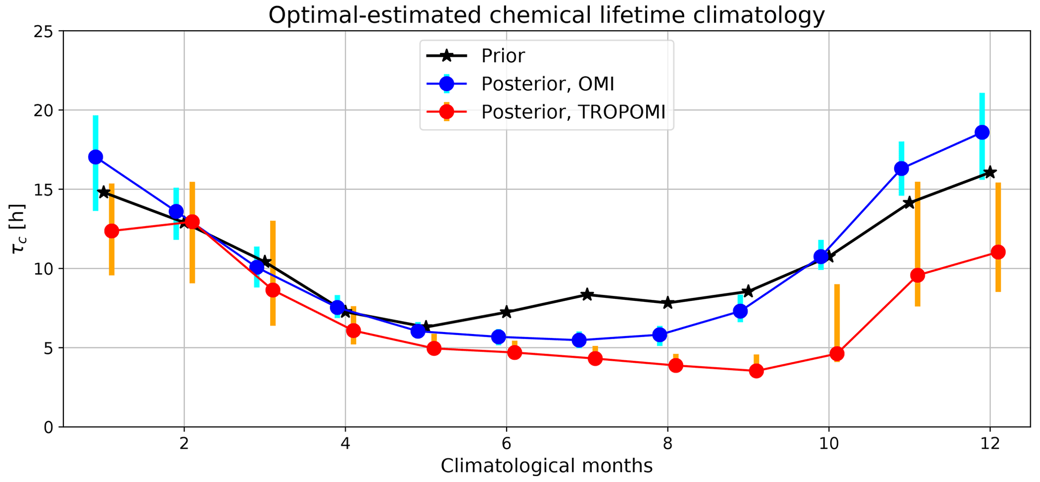
Figure 9 Prior (black) and posterior (blue for OMI and red for TROPOMI) climatological chemical lifetimes from optimal estimation. The prior chemical lifetimes are based on nonlinear fitting to the climatological column–wind speed relationships. The error bars indicate 95 % confidence intervals by bootstrapping the calendar months used to construct each climatological column–wind speed relationship.

The TROPOMI-based climatological chemical lifetimes are suspiciously low after September. As the NO_x sinks are driven by ambient temperature and solar radiation, we do not expect lower chemical lifetimes in September–October than June–July. This anomaly likely results from abnormal TROPOMI column–wind speed relationships characterized by high NO₂ TVCDs in a few wind speed bins. Although the individual monthly column–wind speed relationship from OMI is noisier than TROPOMI (Fig. 3), the much longer OMI record (201 calendar months vs. 38 calendar months for TROPOMI) enables more effective removal of outlier months and retrieval of climatological chemical lifetimes. As such, we focus on the OMI-based chemical lifetime climatology for the following analysis. The NO_x climatological chemical lifetimes are 5–6 h in summer and 15–20 h in winter, generally consistent with CTM studies that consider NO_x sinks comprehensively (Mijling and Van Der A, 2012; Stavrakou et al., 2013; Silvern et al., 2019; Shah et al., 2020). The summertime NO_x chemical lifetime is also close to or slightly higher than other observational-data-driven estimates, mostly through fitting the downwind decay of NO₂ plumes (Valin et al., 2013; de Foy et al., 2015; Liu et al., 2016; Goldberg et al., 2019a; Laughner and Cohen, 2019). This is consistent with the modeling verification by de Foy et al. (2014), which found the NO_x chemical lifetime derived from the EMG-based approach to be biased low compared to the true lifetimes in the model simulations.

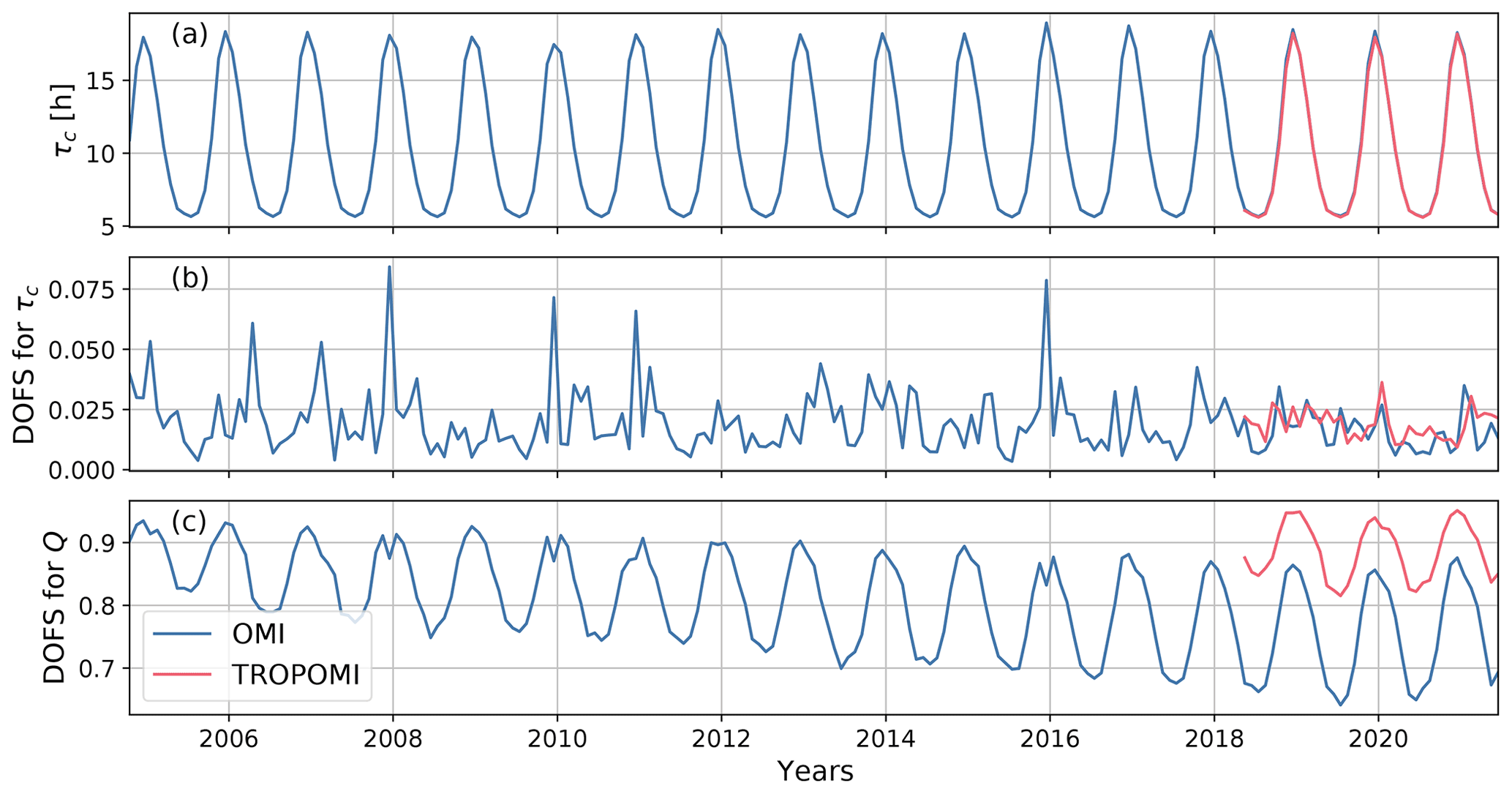
Figure 10 Time series of chemical lifetime (a), degrees of freedom for signal (DOFS) for chemical lifetime τ_c (b), and DOFS for emission rate Q (c) from the calendar-month-based optimal estimations using OMI (blue) and TROPOMI (red) monthly data.

The OMI-based climatological chemical lifetimes in Fig. 9 are then used as priors to derive chemical lifetimes in each calendar month for both OMI and TROPOMI. The resultant monthly NO_x chemical lifetimes are shown in Fig. 10a. Note that the chemical lifetimes in Fig. 10a are retrieved from column–wind speed relationships for each calendar month, whereas the chemical lifetimes in Fig. 9 are retrieved from column–wind speed relationships for each climatological month. The degrees of freedom for signal (DOFS) of retrieved emission rates and chemical lifetimes, shown by Fig. 10b and c, are the diagonal elements of the averaging kernel matrix as given in Appendix B. The DOFS quantifies the number of pieces of information retrieved from observations for a specific state vector element (Rodgers, 2000; Brasseur and Jacob, 2017). The observational information content of τ_c for each calendar month, as indicated by the DOFS, is only ∼0.02 (Fig. 10b). This implies that the chemical lifetimes for calendar months are dominated by prior influences from the climatological chemical lifetimes, which reflects our trade-off between emission rates and chemical lifetimes by applying relatively strong prior regularization to τ_c in each calendar month. While the climatological chemical lifetimes are also derived from observations, the lack of observational constraints for the lifetime in each individual calendar month makes them closely resemble the corresponding climatological month values (i.e., the prior) and prevents us from further interpretation of these monthly lifetime values.

The information on the retrieved emission rate Q that is gained from observations, indicated by the corresponding DOFS, is, however, high and close to unity (Fig. 10c). This indicates that we can confidently retrieve emission rates from the monthly column–wind speed relationships. The decaying DOFS for OMI-based emission rates from 2004 to 2021 is likely due to the gradual increase in OMI radiance noise (Schenkeveld et al., 2017) and consequently increased uncertainties in OMI NO₂ TVCD. The higher DOFS from TROPOMI than OMI is also consistent with the instrument performances.

4.3 Observational constraints on the NO_x : NO₂ ratio

Despite its limited effect on the estimates of NO_x chemical lifetime and relative emission changes, the uncertainty of the NO_x : NO₂ ratio (ϕ in Eq. 5) will directly propagate to the NO_x emission rate estimates. We investigate the ground-based NO_x : NO₂ ratio measured at EEA sites as labeled in Fig. 11a. No ratio data are available in the most polluted Milan metropolitan area because only NO₂ data are reported. Figure 11b shows the monthly distribution of the NO_x : NO₂ ratio in the Po Valley as grayscale background and the monthly median values as a red line. The data coverage is sparse in 2015–2017, and no sensible temporal variation can be identified. Consistent seasonal variation of the NO_x : NO₂ ratio is observable in 2018–2021 with high values (1.5–1.6) in the winter and low values (1.2–1.3) in other seasons, with the caveat that the data after 2020 are not fully validated. The ratios in 2013 and 2014 show a similar seasonal pattern but broader distributions and higher median values in the warm months. Given this discontinuity, we cannot draw a conclusion about the interannual trend of the NO_x : NO₂ ratio. Nonetheless, the seasonal pattern is robust and consistent with low photochemical reactivity in the winter. Therefore, we average the monthly NO_x : NO₂ ratios in 2013–2014 and 2018–2019 and use them as a climatology.

Figure 11 (a) Black circles are the locations of ground-based observation sites where NO_x and NO₂ data are available. TROPOMI NO₂ TVCD from May 2018 to May 2019 oversampled to a 0.02^∘ grid is illustrated in the background. (b) The background shows the density of available NO_x : NO₂ ratios from filtered hourly ground-based measurements. The red line shows the monthly median values.

4.4 NO_x emission rates

Figure 12 presents the monthly air-basin-scale emission rate retrieved from OMI and TROPOMI column–wind speed relationships. The long-term trend and seasonality of OMI-based emission rates generally match those from the JPL chemical reanalysis (r=0.40). The emission rates from bottom-up inventories EDGAR, PKUNOx, and CEDS are also shown in Fig. 12; EDGAR is only available as annual average. We use the surface total NO_x emissions from the JPL chemical reanalysis, which does not include lightning (1.8 % of surface total). According to the JPL chemical reanalysis, 96.2 % of surface total NO_x emissions are anthropogenic. All sectors from CEDS, EDGAR, and PKUNOx are used. Although the PKUNOx and CEDS inventories are monthly, their seasonality differs significantly from the OMI-based and JPL chemical reanalysis values. The interannual trends agree reasonably well between bottom-up inventories and top-down emission estimates (JPL chemical analysis and this study) in their overlapping periods, although the emission decrease trends are not as strong in the top-down estimates as in the bottom-up estimates. The JPL chemical reanalysis reports 3.5 % of NO_x emissions in the Po Valley from soils. However, other top-down studies indicate that the soil emissions may be underestimated in Europe, ranging from 14 % to 40 % (Visser et al., 2019, and references therein). Since the satellites observe emissions from all sources, the discrepancy may also be from missing soil NO_x emissions in bottom-up inventories. The TROPOMI-based emission rates show similar variation as OMI and the JPL chemical reanalysis, but tend to be lower than OMI in the cold months and higher than OMI in the warm months. The calendar month chemical lifetimes retrieved from TROPOMI are similar to OMI (Fig. 10a), and hence the differences in OMI- and TROPOMI-based emission rates directly result from differences in their NO₂ TVCDs. This is supported by Fig. 3; when wind speed is controlled, the OMI TVCDs are higher in cold months, while the TROPOMI TVCDs are higher in warm months.

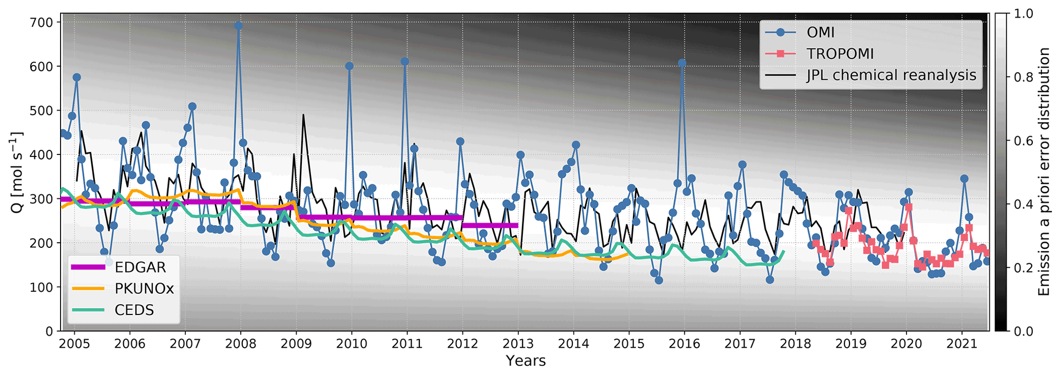
Figure 12 Po Valley NO_x emission rates retrieved from OMI (blue circles) and TROPOMI (red squares) column–wind speed relationships in each calendar month. Monthly emission rates calculated from the JPL chemical reanalysis, EDGAR, PKUNOx, and CEDS inventories are shown as black, magenta, yellow, and cyan lines. The background color map indicates the prior error distributions normalized to the peak height of unity for each calendar month.

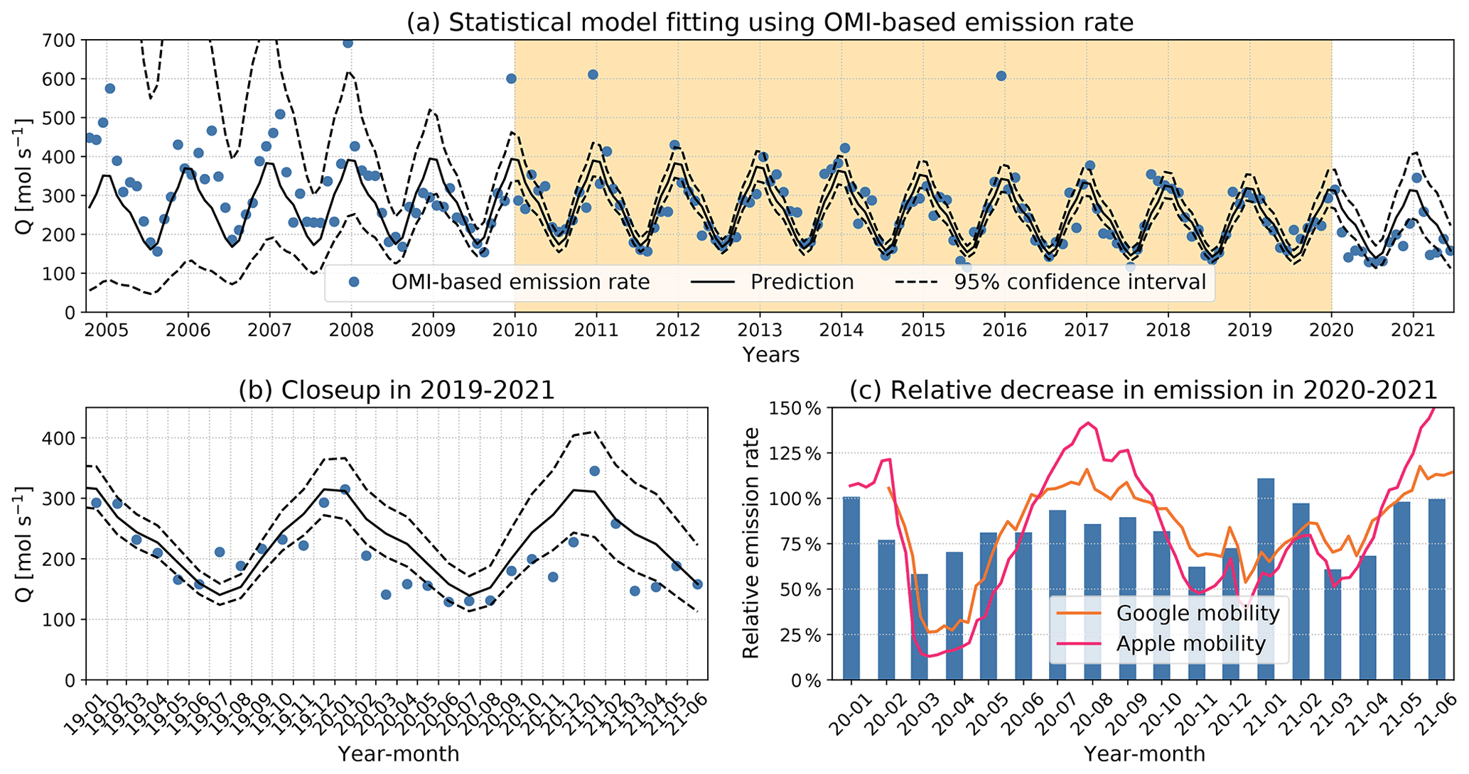
Figure 13 (a) The blue dots show the monthly OMI-based emission rates. The black solid and dashed lines show the prediction and 95 % confidence intervals using the model as in Eq. (6). Only data points for 2010–2019 (yellow shade) are used to fit the model. Prediction values outside this range are extrapolations. Panel (b) is similar to (a) but focused on the period after 2019. (c) The bars show real 2020–2021 emission rates relative to the predicted emission rates. The yellow and red lines show Google and Apple mobility indicators.

Once the air basin length scale is selected (see Sect. 4.1), the proposed satellite-data-driven framework can be used to quantify rapid emission perturbations. The Po Valley region experienced three major COVID-19 outbreaks, and the condition is still evolving (Dong et al., 2020). All outbreaks triggered lockdown measures that are expected to reduce NO_x emissions. However, the quantitative measure of net emission reduction due to the lockdowns is complicated by the long-term decreasing trend and intra-annual variability. For instance, the simple difference between 2020 and 2019 values includes both the pandemic-induced emission changes and the business-as-usual decrease. Leveraging the long and consistent OMI record, we train a statistical model to present the interannual and intra-annual variability using the OMI-based emission rates from January 2010 to December 2019 (yellow shaded region in Fig. 13a):

$$\begin{array}{}\text{(6)}& \begin{array}{rl}& Q\left(t\right)=\\ & \exp \left(\sum _{i=\mathrm{0}}^{n_{\mathrm{p}}}\left(c_i{t}^i\right)+\sum _{j=\mathrm{1}}^{n_{\mathrm{h}}}\left(a_j\sin \left(\mathrm{2}\mathit{\pi }tj\right)+b_j\cos \left(\mathrm{2}\mathit{\pi }tj\right)\right)+e\right),\end{array}\end{array}$$

where t is time measured in fractional years resolved by month, c, a, and b are model parameters, and e is an error term. The order of polynomial n_p=3 and the number of harmonics n_h=4 are chosen through the Akaike information criterion (Akaike, 1974). The fitted model and 95 % confidence intervals are estimated using ordinary least squares and displayed in Fig. 13a and b. Because the model fitting does not involve data before 2010 or after 2020, the model line over those years is from extrapolation and characterized by increasingly large uncertainties (i.e., broader confidence intervals) as the range of projection grows. The well-documented emission perturbation during the 2008–2009 financial crisis (Castellanos and Boersma, 2012) is evident in the discrepancy between model extrapolation and real emission rates (Fig. 13a). Similarly, since this statistical model is trained using data before the pandemic, the prediction in 2020 and beyond serves as a business-as-usual baseline. Compared to just using a previous year or multiyear averaged climatology as a reference (Goldberg et al., 2020; Liu et al., 2020; Bauwens et al., 2020), the model prediction incorporates both the long-term trend and seasonality and is less sensitive to noise in monthly estimates. The real emission rates during the pandemic relative to the predicted emission rates are shown in Fig. 13c. Significant COVID-19-induced emission reduction started in February 2020 and peaked in March 2020 at 42 %. The emission rate gradually recovered as the first outbreak was under control and reached 85 %–95 % of the pre-existing trajectory in June–September 2020. Thereafter, the emission rate dropped twice as of July 2021, reaching reductions of 38 % and 39 % relative to the no-pandemic scenario in November 2020 and March 2021. These reductions correspond to the second and third outbreaks with the subsequent controlling measures. The emission rates in January–February and May–June 2021 seem to be back to the expected normal, highlighting the evolving nature of pandemic-induced emission perturbations. Overall, the real annual emission of 2020 is estimated to be 22 % lower due to the net effect of the COVID-19 pandemic in the Po Valley air basin.

We further correlate the COVID-19-induced NO_x emission changes with the qualitative indicators of human activities estimated by the mobility of Google (Google LLC, 2021) and Apple (Apple, 2021) users. The Google mobility is measured by aggregated Google user activity levels for the categories grocery and pharmacy, parks, transit stations, workplaces, and retail and recreation relative to a baseline period during 3 January–6 February 2020. Google mobility reported for six Italian regions in the Po Valley air basin, including Piedmont, Lombardy, Veneto, Liguria, Emilia–Romagna, and Friuli–Venezia Giulia, is averaged. The Apple mobility is measured by Apple user activity levels in driving and transit modes over the entirety of Italy relative to the baseline on 13 January 2020. Both Google and Apple mobility indicators are in daily native resolution and averaged weekly to remove day-of-week effects. The result is shown in Fig. 13c. The relative NO_x emission changes and the mobility indicators consistently show the three troughs corresponding to large outbreaks. The impacts of the second and third outbreaks were lower than the first one, which is also consistent between the mobility indicators and OMI-based net emission changes. Discrepancies are noted in April 2020 and January 2021, when the mobility indicators stayed low after major control measures, but the NO_x emissions recovered quicker. We speculate that this is the impact of industrial NO_x emissions that are not well represented by the human mobility indicators.

5 Conclusions and discussion

We present a satellite-data-driven framework to rapidly quantify NO_x emission rates over an air basin and demonstrate it in the Po Valley, Italy. Monthly emission rates and chemical lifetimes of NO_x are retrieved from observed column–wind speed relationships, wherein the NO_x column abundance is represented by OMI and TROPOMI NO₂ TVCD observations, and the wind speed is obtained from ERA5 reanalysis. To regularize the retrieval, we derive a NO_x chemical lifetime climatology and use it as prior information. The NO_x chemical lifetime is 5–6 h in summer and 15–20 h in winter. Our observation-based emission rate estimates are consistent with top-down and bottom-up inventories and can be quickly updated as the method only depends on satellite and reanalysis data. Leveraging the long and consistent OMI record, a statistical model is trained to predict the business-as-usual trajectory without the pandemic. Compared with this trajectory, the real 2020–2021 emission rates show three distinctive dips that correspond to tightened COVID-19 control measures and reduced human activities. The overall net NO_x emission reduction due to the COVID-19 pandemic is estimated to be 22 % in 2020 with maximum reduction in March, followed by November. The pandemic-induced emission reduction continued in March–April 2021.

Only observations under modest wind (3–8 m s⁻¹) are used, so there is an implicit assumption that NO_x emissions under modest wind can represent all wind conditions. Since NO_x sources in air basins are mostly anthropogenic, this assumption is deemed to be valid. In addition, the satellite observations are made in the early afternoon local time, so the retrieved emission rates may not necessarily represent the diurnal mean emission rate. This is a common limitation of all observational-data-driven approach, and we note that the overall emission rate level is anchored to the overall emission rate level of the JPL chemical reanalysis, which is spatiotemporally complete, through the selection of basin length scale L. The uncertainties of the retrieved monthly emission rates may also originate from the systematic biases of NO₂ TVCD products, but the relative emission variations should be insensitive to the observational biases. Updated satellite products (e.g., the version 2 TROPOMI NO₂ product to be released in 2021) can be readily adopted. The monthly climatological NO_x : NO₂ ratio derived from ground-based observation networks is used to convert NO₂ abundance to NO_x abundance, which improves upon the fixed value used in previous studies (Beirle et al., 2011; Valin et al., 2013; de Foy et al., 2015; Liu et al., 2016). However, uncertainty remains from contamination of NO₂ in situ measurements (Visser et al., 2019) and the representativeness of the surface-based NO_x : NO₂ ratio to the column-integrated one due to proximity to emission sources and local ozone titration. Moreover, a long-term trend in NO_x : NO₂ may exist, as observed in the Netherlands by Zara et al. (2021), although biases in NO_x : NO₂ have limited impacts on chemical lifetime and relative emission change estimates. The seasonal variability of estimated NO_x emissions is determined by the seasonal variabilities of NO₂ TVCD, chemical lifetime, and the NO_x : NO₂ ratio. We attempt to characterize these variabilities using as much observational data as possible, and yet future investigations are still needed. The general framework is not limited to NO₂ and NO_x in the Po Valley air basin, but can be applied to investigating the emissions and lifetimes of other short-lived species in other geographical regions.

Appendix A: Pixel-based comparison between OMI and TROPOMI NO₂ TVCDs

The TROPOMI retrievals within ±1 h from an OMI retrieval are averaged using the relative pixel overlapping area as weight, and only OMI pixels that are >80 % covered by such TROPOMI pixels are used for comparison. This ensures that OMI and TROPOMI sample essentially the same air mass, and the NO₂ differences reflect the inherent differences of those two products. Figure A1 compares the strictly collocated OMI and TROPOMI retrievals from December 2019 to November 2020. Since the TROPOMI value in each TROPOMI–OMI pair is weight-averaged by 10–90 TROPOMI pixels, its random error is significantly lower than the OMI value, and hence we use the slope in ordinary least square (OLS) regression to represent the OMI $/$ TROPOMI ratio.

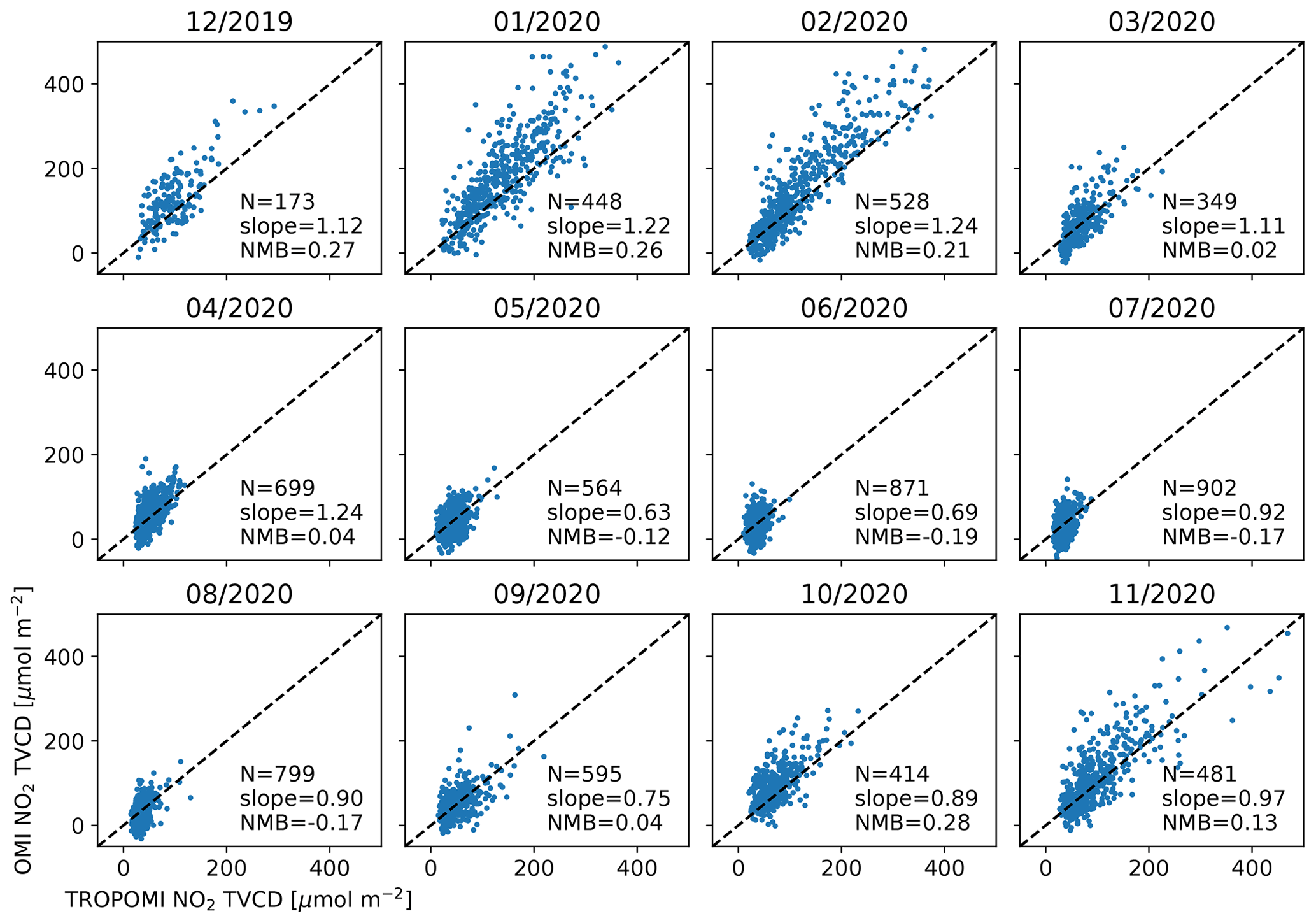
Figure A1 Correlation plots between weight-averaged TROPOMI NO₂ TVCD at OMI pixels and the corresponding OMI NO₂ TVCD; 1 year of data from December 2018 to November 2019 are shown monthly for each panel. The number of collocation pairs (N), OMI $/$ TROPOMI slope from OLS regression, and OMI–TROPOMI NMB are shown in each panel. The dashed black line is 1:1.

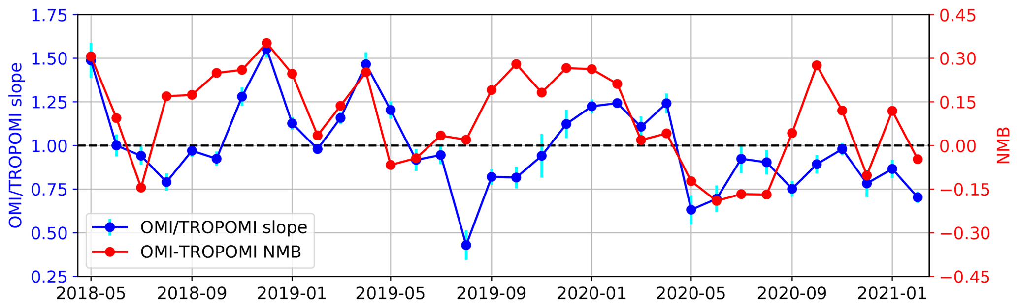
Figure A2 OMI $/$ TROPOMI OLS slope (blue) and OMI–TROPOMI NMB (red) for each month when TROPOMI NO₂ TVCD data are available for comparison.

Figure A2 compares both the OLS slope and the OMI–TROPOMI NMB. In general, OMI is higher than TROPOMI in the cold season, as indicated by slopes larger than unity and NMB larger than zero, whereas TROPOMI is higher in the warm season. The temporal variation of the OLS slope and NMB shows only moderate correlation (correlation coefficient r=0.54), indicating that the discrepancy between OMI and TROPOMI is more complicated than a zero-level offset or proportional scaling.

Appendix B: Details in optimal estimations of Q and τ_c

This Appendix provides technical details on the optimal estimation using column–wind speed relationships over both climatological months (Sect. 3.3.2) and calendar months (Sect. 3.3.3)

Separately for OMI and TROPOMI, the column–wind speed relationship 〈Ω〉 vectors are concatenated to a single observational vector (y):

$$\begin{array}{}\text{(B1)}& \mathit{y}=[\langle \mathbf{\Omega }\rangle (\mathrm{month}\mathrm{1}),\langle \mathbf{\Omega }\rangle (\mathrm{month}\mathrm{2}),\mathrm{\dots }].\end{array}$$

There are 12 months for the climatology retrieval, 201 months for OMI-based calendar month retrieval, and 38 months for TROPOMI-based calendar month retrieval. The state vector β includes emission rates and chemical lifetimes of all months:

$$\begin{array}{}\text{(B2)}& \begin{array}{rl}\mathit{\beta }& =\left[Q\right(\mathrm{month}\mathrm{1}),Q(\mathrm{month}\mathrm{2}),\mathrm{\dots },{\mathit{\tau }}_{\mathrm{c}}(\mathrm{month}\mathrm{1}),\\ & {\mathit{\tau }}_{\mathrm{c}}\left(\mathrm{month}\mathrm{2}\right),\mathrm{\dots }].\end{array}\end{array}$$

The optimal estimation is obtained by iteratively minimizing the cost function

$$\begin{array}{}\text{(B3)}& \begin{array}{rl}J& =(\mathit{y}-\mathit{f}(\mathit{\beta }\left){)}^T{\mathit{\lambda }}^{-\mathrm{1}}\right(\mathit{y}-\mathit{f}\left(\mathit{\beta }\right))\\ & +(\mathit{\beta }-{\mathit{\beta }}_{\mathit{a}}{)}^T{{\mathbf{S}}_{\mathbf{a}}}^{-\mathrm{1}}(\mathit{\beta }-{\mathit{\beta }}_{\mathit{a}}).\end{array}\end{array}$$

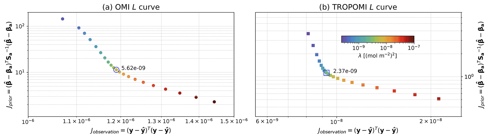
Here f(β) is the forward model by concatenating Eq. (5) for each month, β_a is the prior vector, and S_a is the prior error covariance matrix. In the optimal estimations applied in this study, the strength of prior regularization is controlled by a single factor λ. A lower λ value, or weaker regularization, leads to smaller residuals but larger deviation from the prior; a higher λ value, or stronger regularization, leads to smaller deviation from the prior but larger residuals. We select λ values for OMI $/$ TROPOMI as well as climatology and calendar months separately by finding the maximum curvature point. The corresponding L-curve plots in the Q/τ_c optimal estimations using column–wind speed relationships averaged to climatological months and in each calendar month are shown in Figs. B1 and B2, respectively. The selected λ values are labeled in the plots.

The cost function J (Eq. B3) is minimized by a Gauss–Newton approach, whereby the state vector is updated in each iteration by the following rule:

$$\begin{array}{}\text{(B4)}& \begin{array}{rl}{\mathit{\beta }}_{\mathit{i}\mathbf{+}\mathbf{1}}& ={\mathit{\beta }}_{\mathit{i}}+({{\mathbf{S}}_{\mathbf{a}}}^{-\mathrm{1}}+{{\mathbf{K}}_{\mathbf{i}}}^T{\mathit{\lambda }}^{-\mathrm{1}}{\mathbf{K}}_{\mathbf{i}}{)}^{-\mathrm{1}}({{\mathbf{K}}_{\mathbf{i}}}^T{\mathit{\lambda }}^{-\mathrm{1}}(\mathbf{y}-\mathit{f}({\mathit{\beta }}_{\mathit{i}}\left)\right)\\ & -{{\mathbf{S}}_{\mathbf{a}}}^{-\mathrm{1}}({\mathit{\beta }}_{\mathit{i}}-{\mathit{\beta }}_{\mathit{a}})).\end{array}\end{array}$$

Here β_i is the state vector estimation in iteration i, and β₀=β_a. ${\mathbf{K}}_{\mathbf{i}}=\partial \mathit{f}\left({\mathit{\beta }}_{\mathit{i}}\right)/\partial {\mathit{\beta }}_{\mathit{i}}$ is the Jacobian matrix at iteration i. Since the forward model is concatenated from the column–wind speed relationship for each month (Eq. 5), and the state vector is concatenated from Q and τ_c for each month, the Jacobian can be constructed using analytical derivations of Eq. (5):

$$\begin{array}{}\text{(B5)}& {\displaystyle }& {\displaystyle \frac{\partial \langle \mathbf{\Omega }\rangle }{\partial Q}}={\displaystyle \frac{\mathrm{1}}{\mathit{\varphi }A\left(\frac{\mathit{W}}{L}+\frac{\mathrm{1}}{{\mathit{\tau }}_{\mathrm{c}}}\right)}},\text{(B6)}& {\displaystyle }& {\displaystyle \frac{\partial \langle \mathbf{\Omega }\rangle }{\partial {\mathit{\tau }}_{\mathrm{c}}}}={\displaystyle \frac{Q}{\mathit{\varphi }A}}{\displaystyle \frac{\mathrm{1}}{{\mathit{\tau }}_{\mathrm{c}}^{\mathrm{2}}{\left(\frac{\mathit{W}}{L}+\frac{\mathrm{1}}{{\mathit{\tau }}_{\mathrm{c}}}\right)}^{\mathrm{2}}}}.\end{array}$$

The convergence is determined by comparing the error variance derivative (Bösch et al., 2015),

$$\begin{array}{}\text{(B7)}& \begin{array}{rl}\mathrm{d}{\mathit{\sigma }}_i^{\mathrm{2}}& =({\mathit{\beta }}_{\mathit{i}\mathbf{+}\mathbf{1}}-{\mathit{\beta }}_{\mathit{i}}{)}^T\left({{\mathbf{K}}_{\mathbf{i}}}^T{\mathit{\lambda }}^{-\mathrm{1}}(\mathbf{y}-\mathit{f}({\mathit{\beta }}_{\mathit{i}}\left)\right)\right.\\ & \left.+{{\mathbf{S}}_{\mathbf{a}}}^{-\mathrm{1}}({\mathit{\beta }}_{\mathit{i}}-{\mathit{\beta }}_{\mathit{a}})\right),\end{array}\end{array}$$

with a threshold that scales with the number of state vector elements.

After an optimal solution is found, the DOFS for each state vector element (Q or τ_c) is the corresponding diagonal element of the averaging kernel matrix:

$$\begin{array}{}\text{(B8)}& \mathbf{A}=\mathbf{I}-{\left({\mathbf{K}}^T{\mathit{\lambda }}^{-\mathrm{1}}\mathbf{K}+{{\mathbf{S}}_{\mathbf{a}}}^{-\mathrm{1}}\right)}^{-\mathrm{1}}{{\mathbf{S}}_{\mathbf{a}}}^{-\mathrm{1}},\end{array}$$

where K is the Jacobian matrix at the final iteration and I is an identity matrix with the same dimension as the state vector.

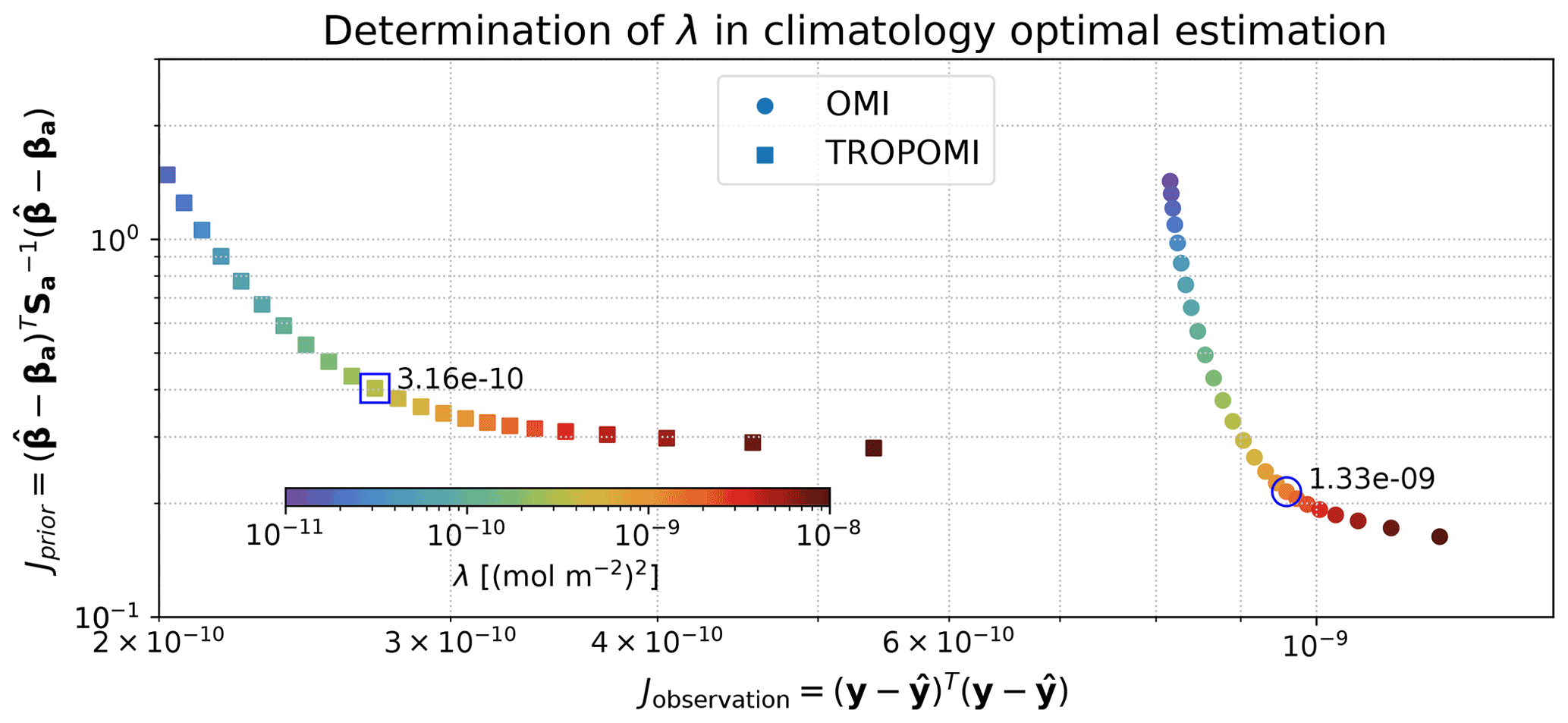
Figure B1 L-curve plot of the squared errors of a regularized solution vs. squared residuals for the climatology of OMI (dots) and TROPOMI (squares).

Figure B2 Similar to Fig. B1 but showing L-curve plots for the optimal estimation for all calendar months for OMI (a) and TROPOMI (b).