the Creative Commons Attribution 4.0 License.
the Creative Commons Attribution 4.0 License.
 | 04 Sep 2020
Comprehensive analyses of source sensitivities and apportionments of PM2.5 and ozone over Japan via multiple numerical techniques
Hikari Shimadera
Syuichi Itahashi
Kazuyo Yamaji
Source sensitivity and source apportionment are two major indicators representing source–receptor relationships, which serve as essential information when considering effective strategies to accomplish improved air quality. This study evaluated source sensitivities and apportionments of ambient ozone and PM2.5 concentrations over Japan with multiple numerical techniques embedded in regional chemical transport models, including a brute-force method (BFM), a high-order decoupled direct method (HDDM), and an integrated source apportionment method (ISAM), to update the source–receptor relationships considering stringent emission controls recently implemented in Japan and surrounding countries. We also attempted to understand the differences among source sensitivities and source apportionments calculated by multiple techniques. While a part of ozone concentrations was apportioned to domestic sources, their sensitivities were small or even negative; ozone concentrations were exclusively sensitive to transport from outside Japan. Although the simulated PM2.5 concentrations were significantly lower than those reported by previous studies, their sensitivity to transport from outside Japan was still relatively large, implying that there has been a reduction in Japanese emissions, similar to surrounding countries including China, due to implementation of stringent emission controls. HDDM allowed us to understand the importance of the non-linear responses of PM2.5 concentrations to precursor emissions. Apportionments derived by ISAM were useful in distinguishing various direct and indirect influences on ozone and PM2.5 concentrations by combining with sensitivities. The results indicate that ozone transported from outside Japan plays a key role in exerting various indirect influences on the formation of ozone and secondary PM2.5 components. While the sensitivities come closer to the apportionments when perturbations in emissions are larger in highly non-linear relationships – including those between NH3 emissions and concentrations, NOx emissions and concentrations, and NOx emissions and ozone concentrations – the sensitivities did not reach the apportionments because there were various indirect influences including other sectors, complex photochemical reactions, and gas–aerosol partitioning. It is essential to consider non-linear influences to derive strategies for effectively suppressing concentrations of secondary pollutants.
- Article
(2722 KB) - Full-text XML
-
Supplement
(2265 KB) - BibTeX
- EndNote


The air quality of Japan has gradually improved. However, ambient concentrations of fine particulate matter smaller than 2.5 µm (PM2.5) and photochemical oxidants (predominantly ozone) exceed the environmental quality standards (EQS). Therefore, we must develop effective strategies to suppress ambient PM2.5 and ozone concentrations. Quantitative source–receptor relationships serve as essential information when considering effective strategies. There are two major indicators representing source–receptor relationships (Clappier et al., 2017). One is source sensitivity, which corresponds to a change in ambient pollutant concentrations caused by a certain perturbation in precursor emissions. The second is source apportionment, which corresponds to the contribution of precursor emissions to ambient pollutant concentrations. Receptor modelling, including chemical mass balance (CMB) and positive matrix factorization (PMF) methods, has been widely applied to evaluate source apportionments (Hopke, 2016). However, these methods have limitations when attempting to treat secondary pollutants, which form in the atmosphere via complex photochemical reactions. Moreover, receptor modelling cannot evaluate source sensitivities. Forward modelling using a regional chemical transport model is a powerful tool for evaluating both the source sensitivities and apportionments of primary and secondary pollutants.
Several numerical techniques have been developed for regional transport models to evaluate source sensitivities and apportionments (Dunker et al., 2002; Cohan and Napelenok, 2011). A simple technique for evaluating source sensitivities is the brute-force method (BFM). Differences in the simulated pollutant concentrations between two simulation cases with and without perturbations in the input precursor emissions are considered to be the sensitivity to a given emission source based on the BFM. This technique can require significant computational resources when evaluating the sensitivities to many emission sources. A decoupled direct method (DDM) is a numerical technique that simultaneously tracks the evolution of sensitivity coefficients, in addition to pollutant concentrations, when solving model equations (Yang et al., 1997). This method has been extended to a high-order DDM (HDDM) to track high-order sensitivity coefficients (Hakami et al., 2003). The ozone source apportionment technology (OSAT) (Dunker et al., 2002) and particulate matter source apportionment technology (PSAT) (Wagstrom et al., 2008) are numerical techniques that evaluate the source apportionments of ozone and particulate matter concentrations, respectively, by tagging contributions of precursor emissions to simulated concentrations. An integrated source apportionment method (ISAM) is a similar numerical technique that evaluates source apportionments (Kwok et al., 2013). Each method has its strengths and weaknesses, such that it is important to appropriately interpret results that will be used to develop effective strategies.
Source sensitivities and apportionments of ambient pollutant concentrations over Japan have been evaluated using regional chemical transport models. Chatani et al. (2011) evaluated the sensitivities of simulated PM2.5 concentrations over three metropolitan areas in Japan to domestic sources and transboundary transport in the 2005 fiscal year. Ikeda et al. (2015) evaluated the sensitivities of simulated PM2.5 concentrations over the nine receptor regions in Japan to source regions in Japan, Korea, and China in 2010. These two studies only employed the BFM to derive source sensitivities of PM2.5 concentrations. Itahashi et al. (2015) evaluated the sensitivities and apportionments of simulated ozone concentrations over East Asia to sources in Japan, Korea, and China. That study presented a unique exercise discussing the differences in source sensitivities and apportionments derived by multiple techniques, including the BFM, HDDM, and OSAT, in Asia; these differences have only been discussed in limited studies targeting the United States and Europe (Koo et al., 2009; Burr and Zhang, 2011; Thunis et al., 2019). Expanding targets is key to obtaining a more comprehensive and appropriate understanding of the source sensitivities and apportionments of pollutant concentrations, including ozone and PM2.5, across Asia, including Japan, derived by multiple techniques.
In addition, recent studies (van der A et al., 2017; Wang et al., 2017; Zheng et al., 2018) suggest that stringent emission controls implemented in China have achieved improved air quality. These improvements should affect air quality not only in China but also across downwind regions including Japan. We must, therefore, update source sensitivities and apportionments when considering additional effective strategies aimed at further air quality improvement in Japan.
Mutual inter-comparisons of the source sensitivities and apportionments derived by multiple models and numerical techniques is one of the objectives of Japan's Study for Reference Air Quality Modelling (J-STREAM) (Chatani et al., 2018b). Model inter-comparisons conducted in earlier phases of J-STREAM have contributed to the derivation of model configurations and development of emission inventories, both of which have contributed to improved model performance (Chatani et al., 2020; Yamaji et al., 2020). As one of the subsequent activities of J-STREAM, this study evaluates the source sensitivities of ozone and PM2.5 concentrations simulated over regions in Japan for a recent year using the outcomes obtained in earlier phases of J-STREAM. Comprehensive analyses from various perspectives were performed to evaluate the sensitivities to eight domestic and two natural emission source groups, as well as foreign anthropogenic emission sources and transboundary transport throughout the entire 2016 fiscal year. In addition, we perform mutual comparisons of the source sensitivities and apportionments of simulated ozone and PM2.5 concentrations. Although the target periods were limited to 2 weeks in four seasons, we discuss notable characteristics with respect to the differences in the source sensitivities and apportionments derived by the BFM, HDDM, and ISAM.
There are well-known non-linear relationships between ambient concentrations of secondary pollutants including ozone and secondary components involved in PM2.5 (Seinfeld and Pandis, 1998). They are likely to cause deviations between source sensitivities and apportionments due to complex photochemical reactions and gas–aerosol partitioning. Nevertheless, it is important to investigate magnitudes of deviations and major causes of non-linear relationships for considering effective strategies to suppress concentrations of secondary pollutants. Processes causing non-linear relationships are universal phenomena and not limited to Japan. The findings of this study contribute not only to solving remaining issues involving ozone and PM2.5 in Japan, but also to understanding of possible influences of non-linear relationships in other countries and regions.
2.1 Model configuration
The Community Multiscale Air Quality (CMAQ) modelling system (Byun and Schere, 2006) version 5.0.2, in which both the HDDM and ISAM are embedded, was selected to calculate the source sensitivities and apportionments, in addition to ambient pollutant concentrations. The carbon bond chemical mechanism with the updated toluene chemistry (CB05-TU) (Whitten et al., 2010) and aero6 aerosol module were employed. Input meteorological fields were simulated by the Weather Research and Forecasting (WRF) – Advanced Research WRF (ARW) version 3.7.1 (Skamarock et al., 2008).
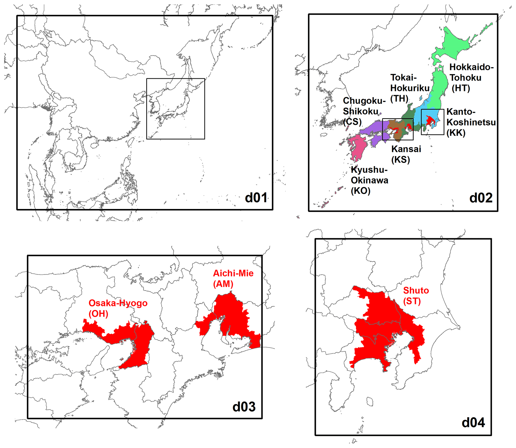
Figure 1Target domains for the simulations in this study. Results are summarized for six colour-coded regions in d02 and three designated areas shown in red in d02, d03, and d04. Their abbreviations are shown in parentheses.
Horizontal locations and resolutions of the four target domains, named d01, d02, d03, and d04, remain unchanged since the first phase of J-STREAM (Chatani et al., 2018b), as shown in Fig. 1. Horizontal resolutions of d01, d02, d03, and d04 are 45 × 45, 15 × 15, 5 × 5, and 5 × 5 km, respectively. The top height of the model was lifted from 10 000 to 5000 Pa to explicitly treat transport in the lower stratosphere (Itahashi et al., 2020). The vertical layer heights were adjusted to be consistent with those of the Chemical Atmospheric Global Climate Model for Studies of Atmospheric Environment and Radiative Forcing (CHASER) (Sudo et al., 2002), which was used to provide boundary concentrations, to avoid numerical diffusions to adjacent layers. Each vertical layer of CHASER from the ground to 80 000 Pa was further divided into two to simulate vertical variations in the lower atmosphere in more detail. The bottom layer height was approximately 28 m.
Several changes were applied to the original WRF configuration employed in the first phase of J-STREAM described in Chatani et al. (2018b) based on the outcomes of the model inter-comparisons. The input land use dataset was replaced with one created from geographic information system (GIS) data based on the sixth and seventh vegetation surveys released by the Biodiversity Centre of Japan, Ministry of Environment, which yielded improved performance for multiple meteorological parameters over urban areas (Chatani et al., 2018a). Lakes were added to the dataset based on the National Land Numerical Information lakes data. The shortwave and longwave radiation schemes were replaced with the Rapid Radiative Transfer Model for General Circulation Models (RRTMG) schemes (Iacono et al., 2008) to use the climatological ozone and aerosol profiles with spatial, temporal, and compositional variations (Tegen et al., 1997). Microphysics and cumulus schemes had significant influences on the simulated pollutant concentrations in the model inter-comparisons. A Morrison double-moment microphysics scheme (Morrison et al., 2009) and Grell–Devenyi ensemble cumulus scheme (Grell and Devenyi, 2002) were newly selected because they were characterized by better performance during the sensitivity experiments. Analysis datasets were replaced with the finer ones, i.e. the NCEP GDAS/FNL 0.25 Degree Global Tropospheric Analyses and Forecast Grids (ds083.3) (National Centers for Environmental Prediction/National Weather Service/NOAA/U.S. Department of Commerce, 2015) and Group for High Resolution Sea Surface Temperature (GHRSST) (Martin et al., 2012), for the initial and boundary conditions, as well as grid nudging. Nudging coefficients are critical parameters for model performance (Spero et al., 2018), but forcing terms in the model equations may disturb physical consistencies. While nudging coefficients for winds were set to 1.0 × 10⁻⁴ s−1 for all domains and vertical layers, those for temperature and water vapour were reduced to 5.0 × 10⁻⁵, 3.0 × 10⁻⁵, 1.0 × 10⁻⁵, and 1.0 × 10⁻⁵ s−1 for d01, d02, d03, and d04, respectively. In addition, nudging for the temperature and water vapour within the planetary boundary layer in d03 and d04 was turned off to avoid excessive nudging to finer spatial and temporal scales than the input analysis datasets, as well as to allow the simulated values to be in accordance with the physical equations.
2.2 Emission inputs
Various improvements were applied to the original emission inputs used in the first phase of J-STREAM described in Chatani et al. (2018b) based on the outcomes of the model inter-comparisons. Hemispheric Transport of Air Pollution (HTAP) emissions version 2.2 (Janssens-Maenhout et al., 2015) was used for anthropogenic sources and international shipping for Asian countries except for Japan. While the target year of HTAP v2.2 is 2010, the ratios of sectoral annual emissions reported by Zheng et al. (2018) were multiplied for China, and those reported by the Clean Air Policy Support System (CAPSS) (Lee et al., 2011) were multiplied for South Korea, to represent the changes in the precursor emissions of recent years. Itahashi et al. (2018) suggested the importance of heterogeneous reactions involving Fe and Mn in sulfate formation. The speciation profiles of Fu et al. (2013) were applied to consider other components, including Fe and Mn, in addition to originally available black and organic carbon in PM2.5 emissions. The PM2.5 emission inventory developed by the Ministry of Environment for the 2015 fiscal year was used for on-road and other transportation sectors in Japan. Emissions from stationary sources in Japan developed in J-STREAM (Chatani et al., 2018b) were fully updated to the 2015 fiscal year with the following improvements. The emission database of large point sources discretized into sectors, facilities, and fuel types was newly developed by Chatani et al. (2019) based on research of air pollutant emissions from stationary sources to represent emissions characteristics and speciation profiles including Fe and Mn. Missing fugitive volatile organic compound (VOC) emission sources, including the use of repellents, air fresheners, aerosol inhalers, cosmetic products, and products for car washing and repair, were added to be consistent with the Greenhouse Gas Inventory Office of Japan (2018). NH3 emissions from fertilizer use and manure management were replaced by the values reported by the Greenhouse Gas Inventory Office of Japan (2018). Fugitive VOC and PM emissions from manure management were newly estimated based on the European Environment Agency (2016). Emission factors of other NH3 sources, including human sweat, human breath, dogs, and cats, were replaced by those reported in Sutton et al. (2000). PM emissions from the abrasion of railways wires and rails were newly estimated as one of the major sources of Fe and Mn. The method to estimate emissions from open agricultural residue burning were replaced by that used by the Greenhouse Gas Inventory Office of Japan (2018). We applied the emission factors reported in Fushimi et al. (2017) and Hayashi et al. (2014), as well as the temporal variations from Tomiyama et al. (2017). Biogenic VOC emissions were estimated by Chatani et al. (2018a) using a detailed database of vegetation and emission factors specific to Japan. The surf zone, defined as zones adjacent to beaches in the National Land Numerical Information Land Use Fragmented Mesh Data, was newly added to estimate higher sea salt emissions from these areas (Gantt et al., 2015) in the CMAQ.
2.3 Simulation setup
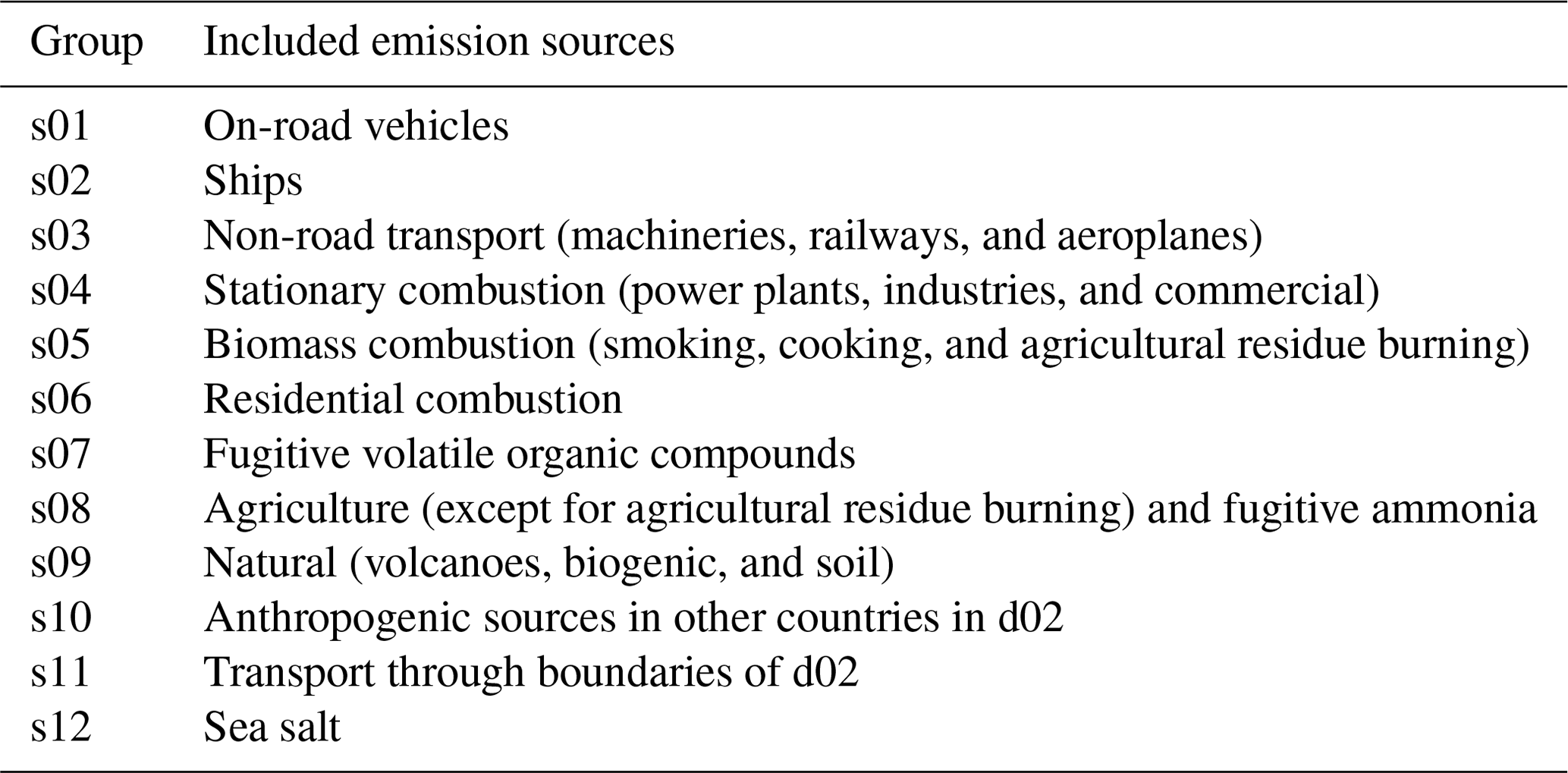
Ambient pollutant concentrations in d01, d02, d03, and d04 were simulated for the entire 2016 fiscal year (from April 2016 to March 2017). Simulations for the preceding month (March 2016) were treated as spin-up. Sensitivities to the emission source groups, classified as listed in Table 1, were evaluated by the BFM, in which the emissions of each source group were reduced by 20 % for the entire fiscal year in d02 and 2 selected weeks in spring (from 6 to 20 May), summer (from 21 July to 4 August), autumn (from 20 October to 3 November), and winter (from 19 January to 2 February 2017) in d03 and d04. These 2 weeks in the four seasons were the periods in which the monitoring campaigns for the ambient concentrations of the PM2.5 components were conducted throughout Japan. The reason for choosing 20 % reduction as a perturbation range in BFM is that it is a typical range of emission reduction by potential emission controls. For s11 (transport through the boundaries of d02), the boundary concentrations of all species for d02 were reduced by 20 %. Differences in the concentrations scaled by 5 between the simulations with and without 20 % perturbations were treated as sensitivities in this study. In addition, source sensitivities and apportionments to all the emission source groups listed in Table 1 were evaluated by the HDDM and ISAM, respectively, using consistent inputs for the 2 coincident weeks in the four seasons in d02. The first- and second-order sensitivity coefficients to gaseous precursors of a single emission source group were calculated using HDDM. We note that the HDDM results were missing for the seasons other than winter because the simulations were not successfully completed because of numerical convergence problems. Table S1 in the Supplement lists the annual total emission amounts for each source group in d02.
Table 1Emission source groups for which sensitivities and apportionments were evaluated in this study.
3.1 Model performance on ozone and PM2.5
We evaluated the model performance for the ozone and PM2.5 concentrations in d02 for the entire 2016 fiscal year. Table S2 in the Supplement lists the statistics for the model performance of the maximum daily 8 h average ozone (MDA8O3) and daily mean PM2.5 concentrations. Table S2 includes the normalized mean bias (NMB), normalized mean error (NME), and correlation coefficient (R) (Emery et al., 2017) for all of Japan (JP), six regions (Kyushu-Okinawa, KO; Chūgoku–Shikoku, CS; Kansai, KS; Tōkai-Hokuriku, TH; Kanto-Kōshin'etsu, KK; Hokkaido–Tohoku, HT), and three areas designated by the automobile NOx–PM law as polluted urban areas (Osaka-Hyogo, OH; Aichi–Mie, AM; Shuto, ST). Figure 1 denotes the locations and abbreviations of the six regions and three designated areas. Automatic continuous monitoring data obtained at the ambient air pollution monitoring stations (APMSs) were used. Figure S1 in the Supplement compares the observed and simulated monthly mean MDA8O3 and PM2.5 concentrations averaged at all stations in the regions.
The MDA8O3 values were slightly overestimated in all regions. The observed MDA8O3 was the highest in May and lowest in December. There was another peak in August in western Japan. The model consistently reproduced these monthly variations. Overestimation occurred from the peak in May to the low in December. Values from December to March were slightly underestimated. The overestimation in summer in this study is less evident than that reported in the study of Chatani et al. (2020), who summarized the performance of the models that participated in the model inter-comparisons conducted in the first phase of J-STREAM. The improved performance obtained in this study may be due to the various improvements in the configurations described in Sect. 2, as well as differences in the meteorological conditions. Kitayama et al. (2019) show that CB05-TU, which was employed in this study, tends to yield lower ozone concentrations among major chemical mechanisms. All the criteria proposed by Emery et al. (2017) were attained in all regions.
The PM2.5 concentrations were underestimated in all regions. The statistics tended to be worse in eastern Japan as opposed to western Japan. The observed PM2.5 concentrations fluctuated with a peak in May and valley near September. Although the simulations reproduced these monthly variations, the absolute values were consistently underestimated. A possible reason is discussed in Sect. 3.2. The criteria proposed by Emery et al. (2017) were attained for NME and R, but not for NMB due to persistent underestimation.
As mentioned in Sect. 2, monitoring campaigns for the ambient concentrations of the PM2.5 components were conducted throughout Japan for the 2 target weeks in spring, summer, autumn, and winter. The components of the particulates collected on filters for 24 h were analysed. These data are useful for the further validation of model performance for the PM2.5 components. Figure S2 in the Supplement shows scatter plots of the observed and simulated daily concentrations of the PM2.5 components (, , , elemental carbon (EC), and organic carbon (OC)) at all locations throughout Japan during the monitoring campaigns in all four seasons. Table S1 summarizes their statistics for all of Japan and the four seasons. The simulated average concentrations of and are similar to the observed values. Their observed and simulated values have significant correlations with R, i.e. approximately 0.7. The concentrations were overestimated with NME of over 100 %. The R between the observed and simulated values is 0.441, which is significantly lower than and . A number of biased dots for occur in the scatter plot. While excessively higher simulated values appeared in summer, the model underestimated several of the higher values mainly observed in winter. Although previous studies have discussed issues of poor model performance associated with reproducing the concentrations in Japan (Shimadera et al., 2014, 2018), they have not yet been solved even after the application of various improvements. Both the EC and OC concentrations were underestimated. As OC is the second major component of PM2.5 following , its underestimation is one of the major causes of PM2.5 underestimation. Shimadera et al. (2018) also discussed the issues of poor model performance associated with reproducing OC concentrations in Japan, suggesting condensable organic matter as a key factor for this poor performance. Although studies on this issue have been conducted by Morino et al. (2018), they remain unsolved.
We note that it is important to recognize that source sensitivities and apportionments introduced in the subsequent sections may be affected by the model performance described in this section.
3.2 Source sensitivities of the annual mean ozone and PM2.5
Figure 2 shows the source sensitivities of the annual mean ozone and PM2.5 concentrations derived by the BFM in all regions. Ozone is overwhelmingly sensitive to s11 (transport through the boundaries of d02). The sensitivities of ozone to domestic sources, including s01 (on-road vehicles) and s04 (stationary combustion), are negative in the three designated areas, which is caused by the titration of ozone because of the higher NOx emissions in urban areas. While the sensitivity of PM2.5 to s11 is the highest, PM2.5 is also somewhat sensitive to domestic anthropogenic sources, including s01, s02 (ships), s04, and s08 (agriculture and fugitive ammonia). The sensitivities to domestic anthropogenic sources are higher in the three designated areas with higher precursor emissions. The sensitivity of PM2.5 to s12 (sea salt) is negative. The sums of the sensitivities of ozone to all the source groups are lower than their simulated concentrations, and the sums of the sensitivities of PM2.5 are higher than their simulated concentrations, due to the non-linear relationships between their concentrations and precursor emissions.

Figure 2Source sensitivities of the annual mean ozone and PM2.5 concentrations derived by BFM in the regions. Thick black lines represent the simulated concentrations.
The sensitivities of PM2.5 reflect the characteristics of the sensitivities of individual PM2.5 components. Figure S3 in the Supplement shows the source sensitivities of the annual mean concentrations of the PM2.5 components derived by the BFM in all regions. The EC and primary organic aerosol (POA) are primary components. Sums of the sensitivities of these primary components to all the source groups are consistent with the simulated concentrations. In the three designated areas (OH, AM, and ST), EC is specifically sensitive to s03 (non-road transport), and POA is specifically sensitive to s05 (biomass combustion). Sums of the sensitivities of , which is mainly a secondary component but almost non-volatile, to all the source groups are also equivalent to the simulated concentrations. is highly sensitive to s09 (natural) in western Japan, i.e. the location of several active volcanoes. Significant non-linearities exist in the sensitivities of and , which are mainly secondary components. Specifically, although s08 mainly emits NH3 but not NOx, concentrations are highly sensitive to it because of the indirect influences. Details of these non-linearities are discussed in Sect. 3.6, which compares the source sensitivities and apportionments. The sensitivities of and to s12 (sea salt) are negative. Cl− originating from sea salts and mostly involved in coarse particles tends to be replaced by because of the so-called chlorine loss caused by gas–aerosol partitioning (Pio and Lopes, 1998; Chen et al., 2016). Therefore, if sea salts are present, more HNO3 gases are partitioned to coarse particles. That provides capacities for and associated involved in PM2.5 to evaporate to the gas phase, resulting in negative sensitivities of PM2.5 including and to sea salts. Non-linearities are also significant to secondary organic aerosol (SOA). SOA is specifically sensitive to biogenic VOC emissions included in s09.
Table S3 in the Supplement lists the ratios of the source sensitivities of the annual mean ozone and PM2.5 concentrations simulated in the regions, which were compared with previous studies. While sums of the ratios of the sensitivities to all the source groups are not 100 % because of the non-linearities, they were often normalized to 100 % in previous studies. Therefore, the ratios normalized to make their sums equal to 100 % are also shown in Table S3. The annual mean PM2.5 concentrations simulated in this study for the three designated areas are 6–9 µg m−3, which is significantly lower than approximately 16 µg m−3 simulated by Chatani et al. (2011) for the corresponding areas in the 2005 fiscal year. However, their ratios of the sensitivities to foreign anthropogenic sources were 48 % in OH, 41 % in AM, and 31 % in ST, which are lower than the approximately 65 % calculated in this study as the sums of the sensitivities to s10 (anthropogenic sources in other countries in d02) and s11. The normalized ratios for the sensitivities to the sources in North and South Korea and China for 2010 were 71 % in Kyushu, 57 % in Kinki, and 39 % in Kanto, reported in Ikeda et al. (2015), whereas in this study the sensitivities to s10 and s11 are 68 % in KO (equivalent to Kyushu), 65 % in KS (equivalent to Kinki), and 59 % in KK (equivalent to Kanto). Relative contributions of foreign sources evaluated in this study are even higher than in previous studies for most areas of Japan despite the stringent emission controls implemented in China.
One of possible reasons for these elevated contributions is reduction of emissions in Japan. Zheng et al. (2018) showed that the emissions of PM2.5, SO2, and NOx in China decreased by 31 %, 52 %, and 15 %, respectively, from 2010 to 2016 as a result of the stringent emission controls. If we compare the emissions reported in Chatani et al. (2011) with those used in this study, which reflected changes in energy consumption and emission controls implemented since 2005, the emissions of PM2.5, SO2, and NOx in Japan decreased by 29 %, 48 %, and 33 %, respectively, from fiscal years 2005 to 2015. Therefore, the relative emission reductions in Japan may be larger than those in China if we assume certain increases in the emissions from 2005 to 2010. In particular, stringent emission controls implemented on diesel vehicles by the central and local governments were quite effective in suppressing PM2.5 emissions and ambient concentrations in urban areas (Kondo et al., 2012). A reduction in the activity of the Miyakejima volcano in recent years has also resulted in lower SO2 emissions. However, we can also state that the underestimations of the PM2.5 concentrations are larger in eastern than western Japan as described in Sect. 3.1. Influences of domestic sources should be accumulated more in eastern than western Japan because the prevalent air flow over Japan is westerly. Therefore, worse model performance in eastern Japan implies underestimation of domestic emissions. Reductions of domestic emissions from fiscal years 2005 to 2015 may be overestimated.
Besides the changes in Chinese emissions, there are other reasons for the higher contributions from sources outside Japan. s11 includes all the components that pass through the boundaries of d02, such that it is affected not only by anthropogenic sources in China, but also by anthropogenic sources in other countries, natural sources, and background concentrations.
Ozone concentrations have been relatively stable in Japan in recent years, while the NOx and VOC concentrations have been suppressed (Wakamatsu et al., 2013). Sensitivities derived in this study suggest that a continuous reduction in the NOx emissions, because of the stringent emission controls implemented in Japan, has resulted in increases in the annual mean ozone concentrations caused by less titration of the ozone in urban areas. Suppressing the annual mean ozone concentrations further is difficult because they are practically insensitive to domestic sources. Trends in the transboundary transport of ozone likely have a significant effect on the mean annual ozone concentrations (Kurokawa et al., 2009; Chatani and Sudo, 2011). In contrast, the annual mean PM2.5 concentrations are sensitive to domestic sources as well as transport from outside Japan. The stringent emission controls implemented in Japan and surrounding countries appear to have contributed to their decreasing trends in Japan. Additional efforts to reduce emissions may produce further improvements in the annual mean PM2.5 concentrations, whereas further validations of the emissions in Japan are necessary.
3.3 Monthly variations in source sensitivities of ozone and PM2.5
Figure 3 shows the source sensitivities of the monthly mean ozone and PM2.5 concentrations derived by BFM simulated for the whole of Japan (JP) and ST, which is one of the three designated areas, including the Tokyo metropolitan area. Figure S4 in the Supplement shows the sensitives of the PM2.5 components. Ozone is negatively sensitive to the domestic sources, including s01 (on-road vehicles) and s04 (stationary combustion), in winter because of the titration of ozone by higher NOx emissions and inactive photochemical reactions in urban areas. The sensitivity of ozone to s11 (transport through the boundaries of d02) is higher than the simulated concentrations, indicating that more ozone is transported from outside Japan and titrated by NOx emissions in Japan. In contrast, negative sensitivities to domestic sources are less evident in summer even in the ST. Reductions in the ozone by titration are compensated for by ozone formation from precursor emissions originating from domestic sources because of the more active photochemical reactions. Differences can be observed in the major source groups, which have positive sensitivities in summer in JP and ST. While the sensitivities of s02 (ships) and s04, which mainly emit NOx, are higher in JP, those of s07 (fugitive VOCs) and s09 (natural), which mainly emit VOCs, are higher in ST.
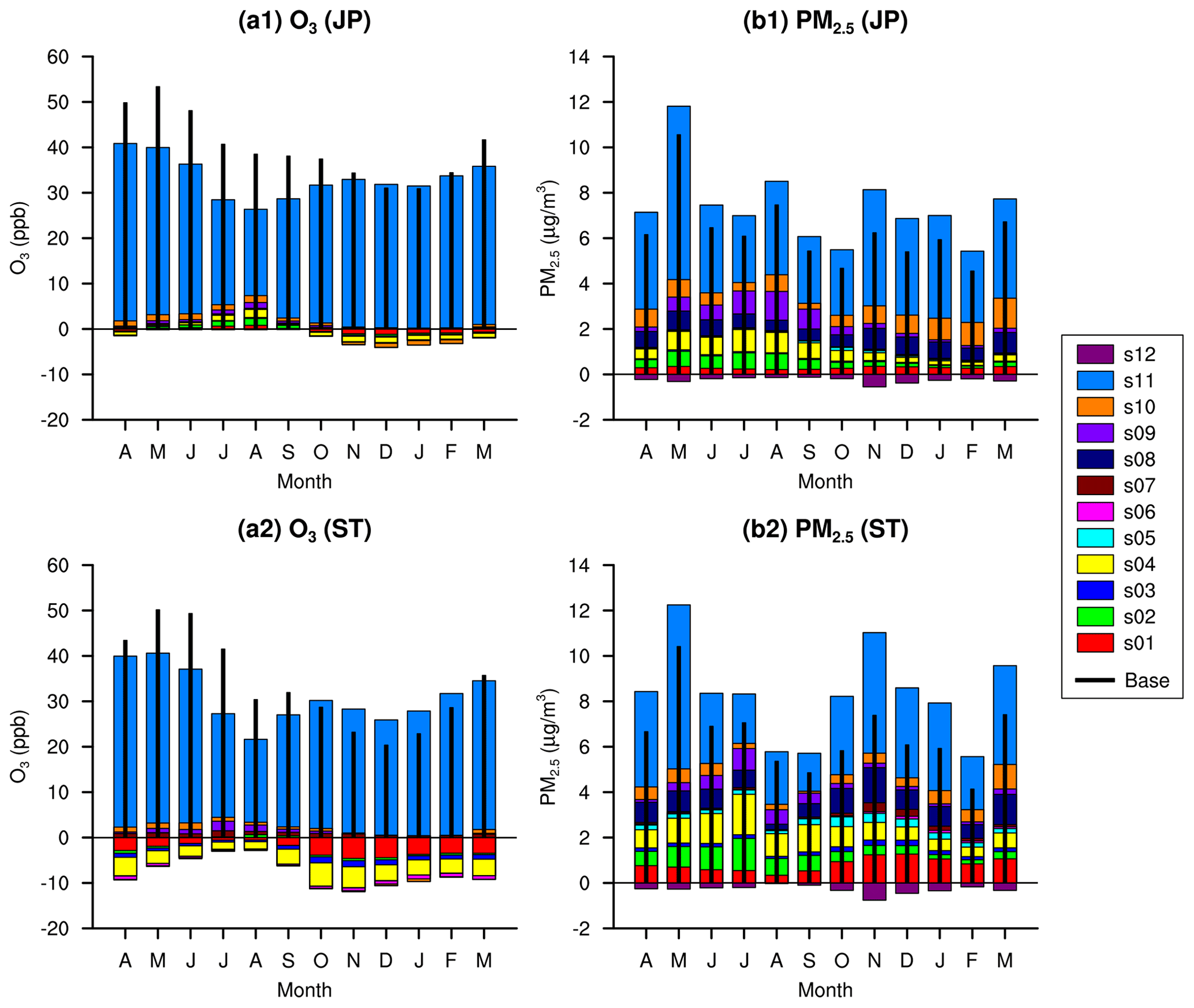
Figure 3Source sensitivities of the monthly mean ozone and PM2.5 concentrations derived by BFM in all of Japan (JP) and ST. Thick black lines represent the simulated concentrations.
The sensitivity of PM2.5 to s11 is the highest in May due to transport by dominant westerly winds in this season. The sensitivity of POA is predominantly high, suggesting that it is affected by variable sources, such as open biomass burning. PM2.5 in summer is highly sensitive to s02, s04, and s09, which are mainly located in the southern sides of Japan, because of dominant southerly winds, as well as active secondary formation, which are clearly reflected in the sensitivities of to these sources. PM2.5 in winter is highly sensitive to s01 and s08 (agriculture and fugitive ammonia). A colder and more stable atmosphere in winter favours the accumulation of emissions from local sources and the partitioning of and to the aerosol phase, as reflected in their sensitivities.
As discussed for the annual mean concentrations, suppressing the monthly mean ozone concentrations is difficult because the sensitivities to s11 are dominant in all months. In particular, the sensitivities to s01 and s04 are largely negative in urban areas in autumn and winter. Further reductions in their NOx emissions may result in additional increases in the monthly mean ozone concentrations in these seasons. In contrast, the negative sensitivities are less evident in spring and summer. Reductions in the precursor emissions for domestic sources have the possibility to suppress, to a certain extent, the monthly mean ozone concentrations. Effective sources may be different in urban and other areas because of differences in ozone formation regimes (Inoue et al., 2019). The effects that strategies have on various sources of precursor emissions for PM2.5 may vary seasonally because of differences in meteorological and photochemical conditions.
3.4 Source sensitivities per unit precursor emissions
Air quality standards are defined in terms of ambient concentrations, whereas targets for emission controls are defined in terms of emission amounts. Therefore, it is important to understand whether the sensitivities of ambient concentrations per equal emission amounts of different sources are consistent or not. Figure 4 shows the sensitivities of the annual mean ambient concentrations of PM2.5 components per annual total amount of corresponding precursor emissions of domestic anthropogenic sources (s01–s08) in all of Japan. All the values shown in Fig. 4 were normalized by the EC value for s01, which is inert and emitted only in the bottom layer. The horizontal and vertical locations of the emissions have an effect on the differences in the values of the primary components (EC and POA). Here, s02 includes ship emissions in surrounding oceans in d02, whose values suggest that approximately 40 % of the ship emissions in d02 affect the concentrations of primary PM2.5 components over Japan. The values for s03 (non-road transport) and s04 (stationary combustion) are slightly lower because they include elevated sources, such as aeroplanes and large point sources. Slight differences among s01 (on-road vehicles), s05 (biomass combustion), and s06 (residential combustion), whose emissions were ingested only in the bottom layer, may be caused by differences in their horizontal distributions. Sources located in coastal areas may have lower influences as their emissions are transported beyond the land. Additional differences caused by photochemical reactions were observed for secondary components. The value for s05 includes agricultural residue burning, which has large spatial and temporal variations, such that its emissions may be high where secondary formation is relatively active. The value of for s01 is significantly higher than that for s08 (agriculture and fugitive ammonia) because s01 co-emits NOx and NH3, which have a mutual correlation.

Figure 4Sensitivities of the annual mean ambient concentrations of PM2.5 components in d02 per total annual amount of corresponding precursor emissions from domestic anthropogenic sources (s01–s08) in all of Japan. All of them are normalized by the EC value for s01.
The effectiveness of equal reduction amounts of the precursor emissions may be different among sources because of photochemical reactions, as well as the locations of emissions. These factors may need to be considered when exploring effective strategies.
3.5 Differences in source sensitivities among domains
Nesting is a technique in air quality simulations aimed at obtaining improved model performance using finer meshes over target regions, as well as representing large-scale transport in coarser meshes in a computationally effective manner. This study employed d03 and d04 with finer 5 km × 5 km meshes over OH, AM, and ST, which include all the major target urban areas. We emphasize the importance of observing how much the sensitivities evaluated in d03 and d04 are different from those in d02 using coarser 15 km × 15 km meshes. Figure 5 shows the sensitivities to all the source groups over OH, AM, and ST evaluated in d02, d03, and d04 averaged for the 2 target weeks during the four seasons. The ozone concentrations simulated for the summer in d02 and d03 or d04 are slightly different. Negative sensitivities to s01 (on-road vehicles) and s04 (stationary combustion) are correspondingly higher. Finer meshes tend to result in slightly larger influences of ozone titration. Although the simulated PM2.5 concentrations are slightly different in different domains, the relative contributions of the source groups to the sensitivities are consistent. These results suggest that differences in horizontal resolutions between d02 and d03 or d04 do not cause critical differences in the sensitivities when they are spatially and temporally averaged over the target areas and 2 weeks. They also support the validity of the discussions in this study, which are mostly based on the results obtained in d02.
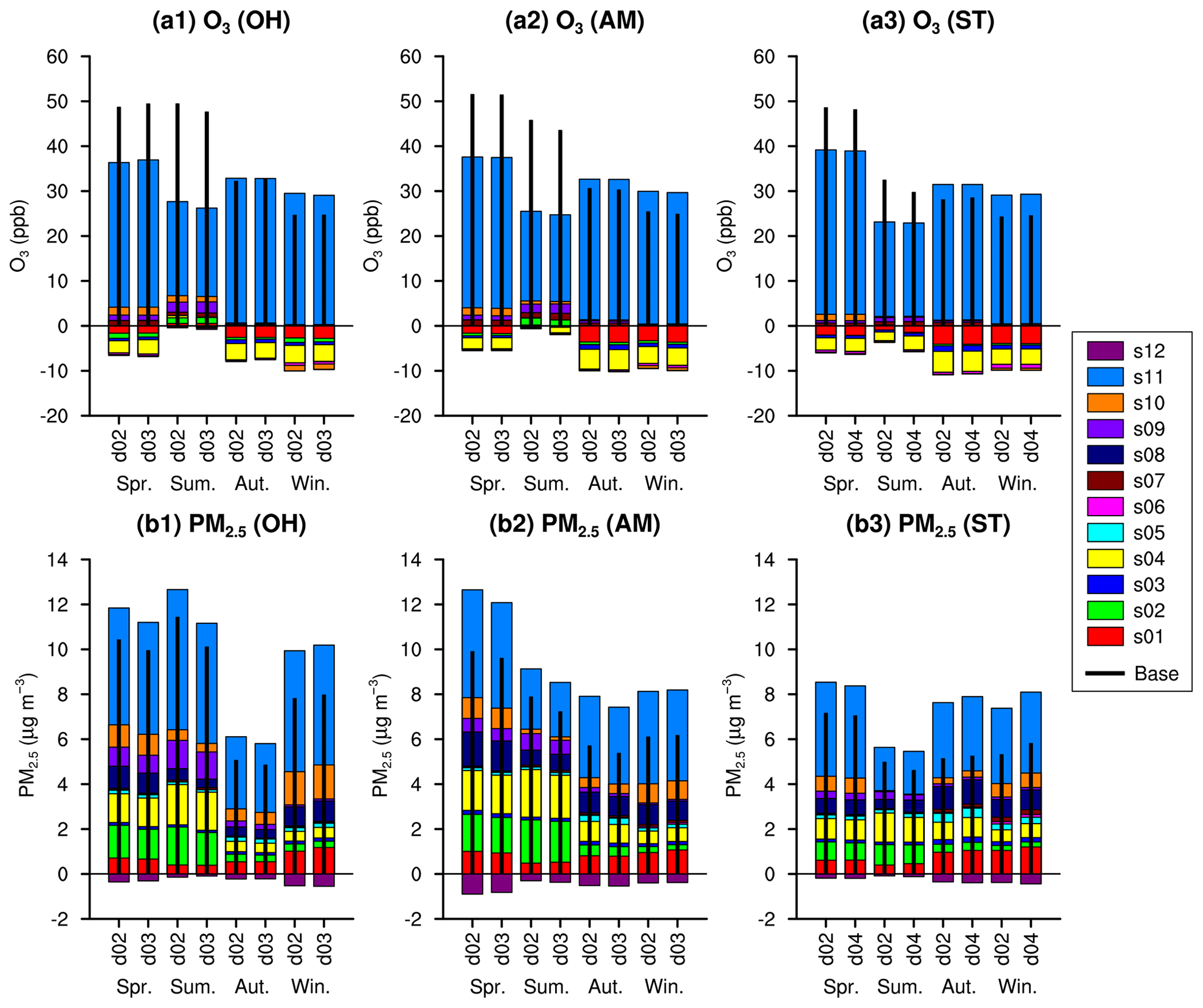
Figure 5Sensitivities of the simulated ozone and PM2.5 concentrations to all source groups over OH, AM, and ST evaluated in d02, d03, and d04 for the 2 target weeks in the four seasons.
3.6 Mutual comparisons of source sensitivities and apportionments derived by BFM, HDDM, and ISAM
3.6.1 Overall differences among techniques
Figure 6 shows the apportionments derived by ISAM and sensitivities derived by BFM and HDDM of the simulated ozone and PM2.5 concentrations to all the source groups for the whole of Japan (JP) and ST averaged for the 2 target weeks during the four seasons. We used the following treatments in Fig. 6. Only the sensitivities to the gaseous precursor emissions were calculated by HDDM. The sensitivities to emissions and boundary concentrations of primary aerosol components (EC, POA, and other primary components) calculated by BFM were also used for HDDM. The simulated SOA concentrations were characterized as apportionments of “OTHR” in ISAM in this study because apportionments of SOA concentrations were not calculated by ISAM embedded in CMAQ version 5.0.2. The HDDM sensitivities were evaluated using first- and second-order sensitivity coefficients (S(1) and S(2)) based on the following Taylor expansion (Eq. 1):
where C(+Δε) and C(0) are the simulated concentrations with and without the perturbations, respectively; Δε is a perturbation ratio; and S(1)(0) and S(2)(0) are the first- and second-order sensitivity coefficients, respectively. The HDDM-20 corresponds to the value calculated by applying and multiplication by 5. If a sensitivity is represented by a second-order polynomial function, HDDM-20 is equivalent to the value obtained by BFM. However, the influence of the second-order term for a perturbation beyond 20 % is not reflected in HDDM-20 because the value at a 20 % perturbation is just linearly extrapolated. They are reflected in the HDDM-100, which corresponds to the value calculated by applying . Differences between BFM and HDDM-20 correspond to the deviations of sensitivities from second-order functions, and differences between HDDM-20 and HDDM-100 correspond to the influences of the second-order term for a perturbation beyond 20 %. Sums of the apportionments of all the source groups derived by ISAM represent, in principle, the simulated concentrations.
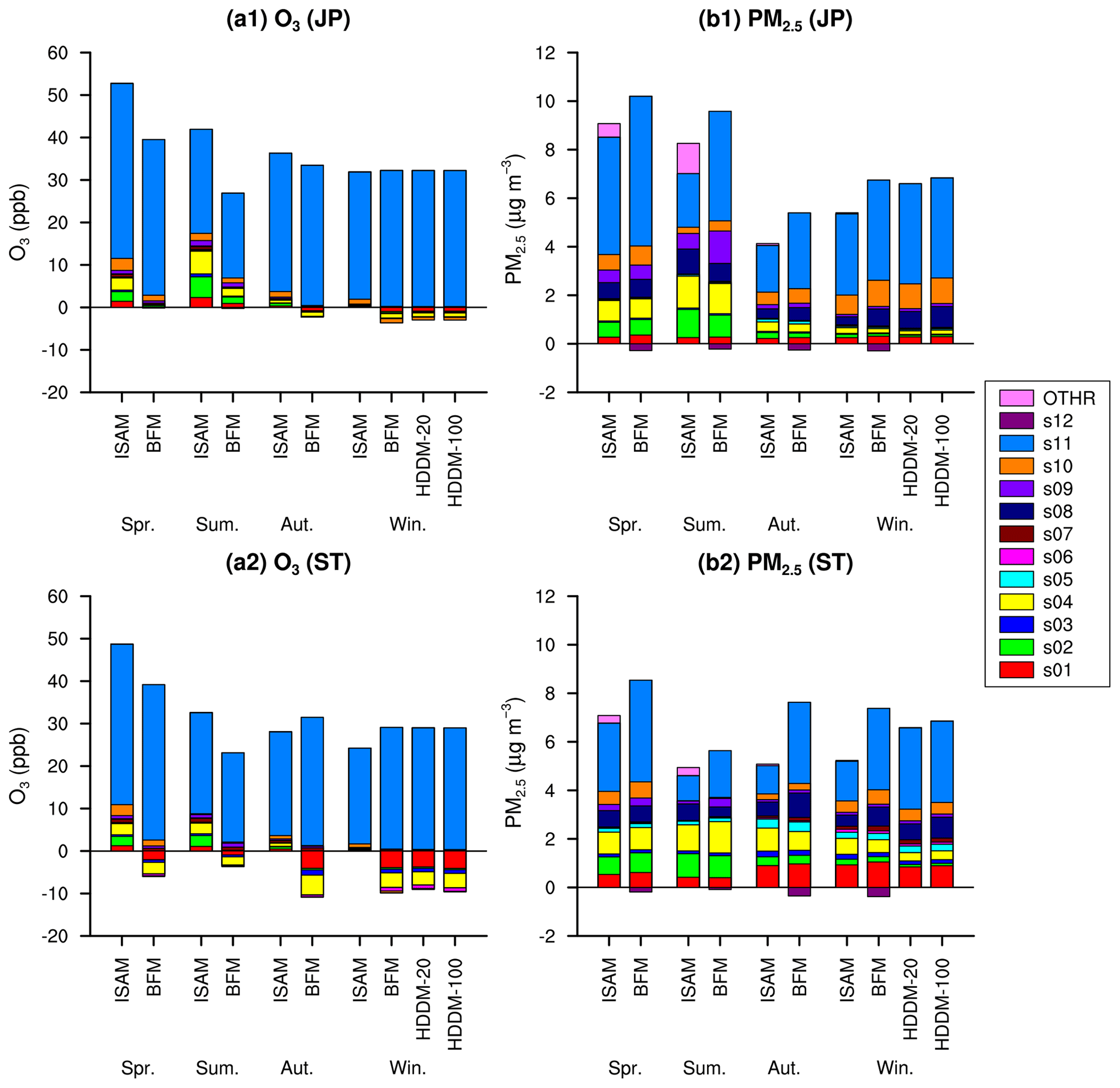
Figure 6Apportionments derived by ISAM and sensitivities derived by BFM and HDDM of the simulated ozone and PM2.5 concentrations to all source groups in JP and ST for the 2 target weeks in the four seasons.
Not only the sensitivities described in previous sections but also the apportionments of ozone to s11 (transport through the boundaries of d02) are dominant, suggesting that ozone over Japan is predominantly transported from outside Japan. There are certain positive apportionments of ozone to domestic sources, including s01 (on-road vehicles), s02 (ships), and s04 (stationary combustion), in the spring and summer, indicating that a certain amount of ozone originates from precursors emitted from these sources. Nevertheless, sensitivities of ozone to domestic sources are small or even negative. Let us consider a simple example. Ozone transported from outside Japan reacts with NO emitted in Japan and forms NO2 (step 1). Next, NO2 is photochemically decomposed to NO and O, followed by ozone regeneration via a rapid reaction between O and O2 (step 2). Potential ozone (ozone + NO2) is preserved in these two steps (Itahashi et al., 2015). Regenerated ozone is apportioned to NO sources in Japan by ISAM in this case. However, if ozone transported from outside Japan increases and enough NO is available, there is a subsequent equivalent increase in NO2 formation and ozone regeneration. This indicates that regenerated ozone is sensitive to transport from outside Japan. In contrast, if NO emissions in Japan increase, ozone concentrations decrease after step 1 or remain unchanged after step 2. This suggests that the sensitivities to NO sources in Japan are negative after step 1 or zero after step 2. Their sensitivities cannot become positive in this example. In reality, a certain amount of the NO is oxidized by other species, including RO2 that originates from VOCs emitted in Japan. They result in net ozone formation and positive sensitivities, which compensates for negative sensitivities to a certain extent. The apportionment of ozone concentrations to s11 is smaller than their sensitivities in autumn and winter in ST. The apportionments to domestic sources are negligible in these seasons. Ozone is titrated by high NO emissions in urban areas in step 1, whereas step 2 is not fully reached because of the inactive photochemical reactions.
There are differences in the source apportionments and sensitivities of PM2.5, which reflect those of the PM2.5 components, shown in Fig. S5 in the Supplement. Sensitivities of gaseous HNO3 and NH3, which are counterparts of and in the gas phase, are also shown in Fig. S5. The source apportionments and sensitivities of primary components (EC and POA) are consistent. While the sums of the source apportionments and sensitivities of to all the sources are also consistent, there are differences in the relative contributions of the source groups. The apportionment to s11 corresponds to the concentrations of transported from outside Japan. The higher sensitivities are affected by additional indirect influences; i.e. SO2 is oxidized to H2SO4 via gaseous and aqueous reactions and is then predominantly partitioned to . Gaseous SO2 is oxidized by OH, a part of which originates in ozone. Therefore, s11, which has an overwhelmingly high sensitivity to ozone, also has higher sensitivities of oxidized from SO2. In contrast, if SO2 emissions are reduced under fixed OH, other SO2 remaining in the atmosphere has the opportunity to be oxidized to . Therefore, the sensitivities to downwind domestic sources are smaller than their apportionments. Similar discussions are applicable to . The apportionments of and HNO3 to s11 are lower than their sensitivities, indicating that a certain amount of the and HNO3 is not directly transported from outside Japan. Ozone overwhelmingly affected by s11 enhances the oxidation of NOx to HNO3 through OH, followed by a smaller amount that is further partitioned to . This causes indirect influences on the sensitivities to s11. Such influences are apparent in the horizontal distributions of the apportionments and sensitivities of concentrations of related species to s11 for the 2 target weeks of spring shown in Fig. S6 in the Supplement. The sensitivities of and are higher than their apportionments over Japan. The sensitivities of SO2 and NO2 over Japan are correspondingly negative, suggesting that they are oxidized by OH that originated in ozone transported from outside Japan. The isolated higher sensitivities over Japan, particularly visible for those of , clearly suggest that they are not directly transported from outside Japan.
Section 3.2 discussed higher relative contributions than previous studies and less contrast between western and eastern Japan for the sensitivities of PM2.5 to s11 obtained in this study. Oxidation of SO2 and NOx emitted from domestic sources by OH that originated in ozone transported from outside Japan is another factor that causes higher sensitivities of s11. The entirety of Japan is equally affected by ozone transported from outside Japan, as shown in Fig. 2a, because of its long lifetime in the atmosphere, resulting in less contrast in the sensitivities of PM2.5 to s11 between western and eastern Japan, whereas the sensitivities of domestic emissions are small. Ozone governs the oxidative capacity of the atmosphere (Prinn, 2003). If ozone transported from outside Japan is not as reduced in future, efforts to reduce SO2 and NOx emissions in Japan will not effectively contribute to the reduction of the concentrations of and because OH that originated in ozone transported from outside Japan affects their formation.
There is no apportionment of to s08 (agriculture and fugitive ammonia), which emits NH3 but not NOx, in accordance with the principle. Nevertheless, is highly sensitive to s08 and is affected by the relationships between and . Here, and are mutual counter ions in NH4NO3, whose formation is enhanced when both are available. More NH3 emissions can induce the partitioning of HNO3 to NH4NO3. These influences can be observed in the correspondingly negative sensitivities of gaseous HNO3 to s08. While the apportionments of are dominated by s08 in ST, its sensitivities are significantly smaller than the apportionments. Both (NH4)2SO4 and NH4NO3 are major forms of , where, as discussed above, NH4NO3 formation is sensitive to NH3 emissions. In contrast, the sensitivities of to s08 are negligible (Fig. S5c2), suggesting that (NH4)2SO4 formation is predominantly limited by SO2 sources, including s02 and s04. Their influences are reflected in the sensitivities of to s02 and s04 (Fig. S5e2). These results are consistent with those of Clappier et al. (2017), who discuss the differences between apportionments and sensitivities in different regimes involving SO2, NOx, and NH3 using idealized example cases.
There is the certain degree of sensitivity of PM2.5 to s08, as shown in Fig. 2b, which is indirectly caused by the interactions between and . There have been several studies that have highlighted the importance of NH3 emission controls to reduce PM2.5 concentrations (Pinder et al., 2007; Wu et al., 2016; Guo et al., 2018). Such discussions are applicable to Japan. However, Liu et al. (2019) suggested that NH3 emission control could worsen acid rain because nitric acid is not neutralized and remains in the atmosphere. When seeking strategies to achieve sustainable developments, it is necessary to consider other environmental aspects, including acid rain and nitrogen cycles, as well as the reduction of PM2.5 concentrations.
3.6.2 Non-linear responses in sensitivities
Differences among the sensitivities derived by BFM, HDDM-20, and HDDM-100 are mostly small, suggesting that, in most cases, HDDM is able to calculate sensitivities consistent with BFM. Slight differences were found in the sensitivities of derived by them. Figure 7a shows the sensitivities of the daily concentrations to the source groups located within d02 (s01–s10) derived by BFM, HDDM-20, and HDDM-100 for the 2 target weeks in winter in ST. The sensitivities derived by BFM are slightly higher than those derived by HDDM-20. While the sensitivities derived by HDDM-20 are only affected by gaseous precursor emissions, those derived by BFM contain minor contributions of primary emitted . They are one of the factors that may result in higher sensitivities derived by BFM. However, differences were found even in the sensitivities to s08 (agriculture and fugitive ammonia), which mostly emits NH3. Differences should be recognized as difficulties in representing sensitivities only with first- and second-order sensitivity coefficients derived by HDDM.

Figure 7(a) Sensitivities of the daily concentrations to the source groups located within d02 (s01–s10) derived by BFM (left), HDDM-20 (middle), and HDDM-100 (right) and (b) daily non-linearity index and available NH3 ratios for the 2 target weeks in winter in ST. Non-linearity indices for first-order sensitivity coefficients less than 0.001 µg m−3 are not shown as they are likely to be affected by numerical noise.
Sums of the sensitivities derived by HDDM-100 are higher than those derived by HDDM-20 for all days, indicating non-linear responses of concentrations against precursor emissions. Daily variations in two additional indicators are shown in Fig. 7b. One is a non-linear index (Cohan et al., 2005), which is calculated as follows:
This corresponds to an absolute ratio of the second- to first-order sensitivity terms when a perturbation is , indicating the strength of the non-linearities. Another indicator is an available NH3 ratio, which corresponds to a ratio of NH3 + (those stoichiometrically equivalent to are subtracted) to HNO3 + , indicating an abundance of potential that can be combined with . Here, s08 has the highest non-linear indices that cause the overall non-linearities, implying that the concentrations have non-linear responses to NH3 emissions. Daily variations in the non-linear indices of s08 and available NH3 ratios are well correlated; non-linearities are higher when available NH3 ratios are lower. The formation of NH4NO3 tends to be more constrained by NH3 with less available NH3, as shown by Xing et al. (2011). A typical situation occurred on 30 January. Negative sensitivities of s04 (stationary combustion) suggest that SO2 emissions of s04 remove NH3 to form (NH4)2SO4 and prevent NH4NO3 formation. The HDDM can represent such complex non-linear relationships involving multiple species.
In addition to BFM with 20 % perturbation (denoted as BFM-20), additional simulations were conducted to derive sensitivities by BFM with 100 % perturbation (denoted as BFM-100) for s04, which emits NOx but not NH3, and s08, which emits NH3 but not NOx. Figure S7 in the Supplement shows the sensitivities derived by BFM-20, BFM-100, HDDM-20, and HDDM-100 and apportionments derived by ISAM of the daily and concentrations to s04 and s08 for the 2 target weeks in winter in ST. The sensitivities derived by BFM-100 are higher than those derived by BFM-20 because of the non-linear responses. Similar features are evident in the sensitivities derived by HDDM-100 and HDDM-20, implying that HDDM is capable of representing directions of non-linear responses beyond 20 % perturbation. It is notable that the sensitivities derived by BFM with a larger perturbation come closer to the apportionments for to s04 and to s08. However, there are still deviations among them caused by indirect influences of factors including other sectors, complex photochemical reactions, and gas–aerosol partitioning. Moreover, and concentrations are never apportioned but non-linearly sensitive to s08 and s04, respectively.
3.6.3 Dependence of ozone formation on NOx and VOC
ISAM has the capability to separately calculate apportionments of ozone to NOx and VOC emissions of a given source based on ozone formation conditions (Kwok et al., 2013). It is important to understand relationships between apportionments and sensitivities of ozone to NOx and VOC emissions. Additional simulations were conducted to separately derive the sensitivities of ozone to NOx and VOC emissions of s01 (on-road vehicles) by BFM with 20 % (BFM-20) and 100 % (BFM-100) perturbations.

Figure 8Sensitivities derived by BFM-20 (left) and BFM-100 (middle) and apportionments derived by ISAM (right) of daily ozone concentrations (shown by a line with markers) to the NOx and VOC emissions of s01 for the 2 target weeks during the summer in ST.
Figure 8 shows the sensitivities derived by BFM-20 and BFM-100 and apportionments derived by ISAM of daily ozone concentrations to the NOx and VOC emissions of s01 for the 2 target weeks in summer in ST. The apportionment to the NOx emissions is higher than the apportionment to the VOC emissions. While there are differences in the magnitudes of the apportionments and sensitivities to the VOC emissions, their daily variations are consistent. The sensitivity to the NOx emissions is mostly negative, but became positive on 25 July when the apportionments, as well as the ozone concentrations, were the highest. The dominant winds were northerly until 24 July and switched to southerly on 25 July. Precursors and the ozone formed from them were transported to the south and returned to ST. Therefore, the aged air mass passed over ST on 25 July. Influences of ozone formation from NOx emissions were higher than the immediate titration by them for this condition.
Figure S8 in the Supplement shows the sensitivities derived by BFM-20 and BFM-100 and apportionments derived by ISAM of the hourly ozone concentrations to the NOx and VOC emissions of s01 on 25 July in ST. Hourly variations in the apportionments and sensitivities to the VOC emissions are consistent. Whereas the sensitivities to the NOx emissions during the night are slightly negative because of titration, their higher positive sensitivities during the daytime indicate the contribution of the NOx emissions to the high ozone concentrations.
We note that the sensitivities to VOC emissions derived by BFM-20 and BFM-100 are almost identical. That means ozone formation from VOCs is linearly related to emissions. The sensitivities of NOx emissions derived by BFM-20 and BFM-100 are also almost identical when they are negative. That means titration of ozone by NOx is also linearly related to emissions. In contrast, the sensitivities to NOx emissions derived by BFM-100 are higher than those derived by BFM-20 when they are positive. That means ozone formation from NOx is non-linearly related to emissions. Cohan et al. (2005) also reported that the sensitivities of ozone concentrations are lower when perturbations of precursor emissions are smaller because other remaining precursors are more likely to contribute to ozone formation instead. This may also be the reason why the sums of the sensitivities to all the sources are lower than the simulated ozone concentrations in spring and summer (Figs. 2, 3, and 5). While the sensitivities derived by BFM-100 come closer to the apportionments, the apportionments are still higher than the sensitivities as discussed for and in Sect. 3.6.2. That implies effects on concentrations of ozone, , and may be less than those inferred by BFM-100 and ISAM when reductions of emissions of NOx and NH3 are small.
Figure S9 in the Supplement shows the horizontal distributions of the apportionments and sensitivities of the ozone concentrations to the s01 NOx and VOC emissions averaged for the 2 target weeks in summer. The sensitivity to NOx emissions is negative in urban and coastal areas where NOx emissions from on-road vehicles are high. There are consistencies in the horizontal distributions of the positive sensitivities and apportionments to NOx and VOC emissions. While there are quantitative differences in the magnitudes of the sensitivities and apportionments due to non-linear influences, ISAM provides spatial and temporal variations in the apportionments to NOx and VOC emissions consistent with the sensitivities derived by BFM.
Sensitivities and apportionments of ozone and PM2.5 concentrations over regions in Japan for the 2016 fiscal year to emissions from 12 source groups were evaluated by the BFM, HDDM, and ISAM using emissions data that take into account the latest stringent emission controls. Ozone was predominantly sensitive to transport from outside Japan. While PM2.5 concentrations were lower than those simulated by previous studies for past years because of emission reductions, the relative contributions of transport from outside Japan to the total sensitivities were even larger, suggesting that emissions in Japan have been reduced similarly to surrounding countries, including China. Moreover, sensitivities of PM2.5 included indirect influences of ozone predominantly transported from outside Japan via the oxidation of precursors by OH to secondary PM2.5 components. There was a certain sensitivity of PM2.5 to domestic sources, but the sensitivity of ozone to domestic sources was significantly smaller or even negative because of titration and non-linear responses against precursor emissions.
Sensitivities and apportionments of primary species were consistent. Fundamental differences were found between them for secondary species. Whereas apportionments represent direct contributions, sensitivities include indirect influences. Clappier et al. (2017) and Thunis et al. (2019) have suggested that sensitivities can provide more useful information than apportionments when considering effective strategies. This study indicates that apportionments simultaneously evaluated with sensitivities can be useful in distinguishing direct and indirect influences; i.e. they cannot be distinguished only by sensitivities. For example, the sensitivities of and to the transport from outside Japan encompassed at least two undistinguished influencing factors, including the direct transport of and , which were evaluated by their corresponding apportionments, and oxidation of SO2 and NOx emitted from domestic sources by OH originating in ozone transported from outside Japan. In addition, the titration of ozone by NOx emissions and inter-correlations between and in their partitioning were also identified as key indirect influences on ozone and PM2.5.
Sensitivities of PM2.5 derived by BFM and HDDM were mostly consistent except for and . There were differences between the sensitivities of and calculated with the first- and second-order sensitivity coefficients derived by HDDM and those derived by BFM. HDDM revealed possibilities to indicate directions of non-linear responses to larger perturbations in emissions. The sensitivities derived by BFM become closer to the apportionments derived by ISAM when perturbations in emissions are larger in highly non-linear relationships, including those between NH3 emissions and concentrations, NOx emissions and concentrations, and NOx emissions and ozone concentrations. However, the sensitivities did not reach the apportionments because of the various indirect influences, including other sectors, complex photochemical reactions, and gas–aerosol partitioning. The dependence of ozone formation on the NOx and VOC emissions derived by ISAM was spatially and temporally consistent with sensitivities derived by BFM.
Understanding the influences that various factors have on sensitivities can contribute to the establishment of effective strategies. However, accurate sensitivities and apportionments depend on model performance. Uncertainties remain in model performance, as discussed in Sect. 3.1. If specific emission sources affect overall model performance, source sensitivities and apportionments derived by models may be skewed. Figure S10 in the Supplement shows source sensitivities of the annual mean PM2.5 concentrations derived by BFM in the regions. The values shown in (b) were uniformly scaled by the ratios of observed and simulated concentrations of PM2.5 components shown in Table S2. The scaled sensitivities of PM2.5 to the transport from outside Japan are higher by 1.0–2.2 µg m−3 (15 %–40 %) because of their high contributions to underestimated POA and SOA. The scaled sensitivities of PM2.5 to other sources are different by 0–0.5 µg m−3. This case assumes that deviations between observed and simulated PM2.5 concentrations can be proportionally explained by the source sensitivities. Uncertainties could be higher if specific sources cause poor model performance. In particular, this study revealed and concentrations are non-linearly sensitive to NH3 and NOx emissions. Uncertainties in NH3 and NOx emission sources could largely influence source sensitivities as well as model performance of and concentrations. More studies are necessary to increase the confidence in source sensitivities and apportionments as well as model performance. In addition, sensitivities obtained by the BFM with a single perturbation may be inappropriate for applications to different perturbation ranges when non-linearities are higher. High-order sensitivity coefficients calculated by the HDDM could help evaluate the importance of non-linear responses.
This study demonstrated that a combination of sensitivities and apportionments derived by the BFM, HDDM, and ISAM can provide critical information to identify key emission sources and processes in the atmosphere. The sensitivities and apportionments were derived with the consistent model configurations and inputs in this study. However, model configurations and inputs may not necessarily be consistent. Itahashi et al. (2019) reported that source sensitivities can be changed by the regional chemical transport model with improved treatments for aqueous reactions. Uncertainties in the sensitivities and apportionments caused by different model configurations and inputs should be explored as the next step of J-STREAM.
The input datasets are available upon request at http://www.nies.go.jp/chiiki/jstream.html (last access: 10 March 2020). The output datasets are available upon request to the authors.
The supplement related to this article is available online at: https://doi.org/10.5194/acp-20-10311-2020-supplement.
SC designed this study, conducted BFM simulations, and prepared the manuscript. HS conducted ISAM simulations, and SI conducted HDDM simulations. KY prepared the meteorology and additional inputs.
The authors declare that they have no conflict of interest.
This study was supported by the Environment Research and Technology Development Fund (JPMEERF20165001 and JPMEERF20185002) of the Environmental Restoration and Conservation Agency of Japan. The data based on the sixth and seventh vegetation surveys were obtained from the Biodiversity Center of Japan, Ministry of the Environment (http://gis.biodic.go.jp/webgis/sc-006.html, last access: 30 January 2017). The National Land Numerical Information data were obtained from the National Land Numerical Information download service (http://nlftp.mlit.go.jp/ksj/index.html, last access: 17 December 2019). Data from the Research of Air Pollutant Emissions from Stationary Sources were provided by the Ministry of the Environment. Automatic continuous monitoring data of the ambient air pollution monitoring stations were obtained from the National Institute for Environmental Studies (http://www.nies.go.jp/igreen/, last access: 21 February 2018). The data associated with the monitoring campaigns for the ambient concentrations of the PM2.5 components were obtained from the Ministry of the Environment (http://www.env.go.jp/air/osen/pm/monitoring.html, last access: 9 July 2019).
This research has been supported by the Environmental Restoration and Conservation Agency of Japan (Environment Research and Technology Development Fund (grant nos. JPMEERF20165001 and JPMEERF20185002)).
This paper was edited by Pedro Jimenez-Guerrero and reviewed by M. Talat Odman and two anonymous referees.
Burr, M. J., and Zhang, Y.: Source apportionment of fine particulate matter over the Eastern U.S. Part II: source apportionment simulations using CAMx/PSAT and comparisons with CMAQ source sensitivity simulations, Atmos. Pollut. Res., 2, 318–336, https://doi.org/10.5094/apr.2011.037, 2011.
Byun, D., and Schere, K. L.: Review of the governing equations, computational algorithms, and other components of the models-3 Community Multiscale Air Quality (CMAQ) modeling system, Appl. Mech. Rev., 59, 51–77, https://doi.org/10.1115/1.2128636, 2006.
Chatani, S. and Sudo, K.: Influences of the variation in inflow to East Asia on surface ozone over Japan during 1996–2005, Atmos. Chem. Phys., 11, 8745–8758, https://doi.org/10.5194/acp-11-8745-2011, 2011.
Chatani, S., Morikawa, T., Nakatsuka, S., and Matsunaga, S.: Sensitivity analyses of domestic emission sources and transboundary transport on PM2.5 concentrations in three major Japanese urban areas for the year 2005 with the three-dimensional air quality simulation, J. Jpn. Soc. Atmos. Environ., 46, 101–110, https://doi.org/10.11298/taiki.46.101, 2011.
Chatani, S., Okumura, M., Shimadera, H., Yamaji, K., Kitayama, K., and Matsunaga, S.: Effects of a detailed vegetation database on simulated meteorological fields, biogenic VOC emissions, and ambient pollutant concentrations over Japan, Atmosphere, 9, 179, https://doi.org/10.3390/atmos9050179, 2018a.
Chatani, S., Yamaji, K., Sakurai, T., Itahashi, S., Shimadera, H., Kitayama, K., and Hayami, H.: Overview of model inter-comparison in Japan's Study for Reference Air Quality Modeling (J-STREAM), Atmosphere, 9, 19, https://doi.org/10.3390/atmos9010019, 2018b.
Chatani, S., Cheewaphongphan, P., Kobayashi, S., Tanabe, K., Yamaji, K., and Takami, A.: Development of Ambient Pollutant Emission Inventory for Large Stationary Sources Classified by Sectors, Facilities, and Fuel Types in Japan, J. Jpn. Soc. Atmos. Environ., 54, 62–74, https://doi.org/10.11298/taiki.54.62, 2019.
Chatani, S., Yamaji, K., Itahashi, S., Saito, M., Takigawa, M., Morikawa, T., Kanda, I., Miya, Y., Komatsu, H., Sakurai, T., Morino, Y., Nagashima, T., Kitayama, K., Shimadera, H., Uranishi, K., Fujiwara, Y., Shintani, S., and Hayami, H.: Identifying key factors influencing model performance on ground-level ozone over urban areas in Japan through model inter-comparisons, Atmos. Environ., 223, 117255, https://doi.org/10.1016/j.atmosenv.2019.117255, 2020.
Chen, Y., Cheng, Y., Ma, N., Wolke, R., Nordmann, S., Schüttauf, S., Ran, L., Wehner, B., Birmili, W., van der Gon, H. A. C. D., Mu, Q., Barthel, S., Spindler, G., Stieger, B., Müller, K., Zheng, G.-J., Pöschl, U., Su, H., and Wiedensohler, A.: Sea salt emission, transport and influence on size-segregated nitrate simulation: a case study in northwestern Europe by WRF-Chem, Atmos. Chem. Phys., 16, 12081–12097, https://doi.org/10.5194/acp-16-12081-2016, 2016.
Clappier, A., Belis, C. A., Pernigotti, D., and Thunis, P.: Source apportionment and sensitivity analysis: two methodologies with two different purposes, Geosci. Model Dev., 10, 4245–4256, https://doi.org/10.5194/gmd-10-4245-2017, 2017.
Cohan, D. S. and Napelenok, S. L.: Air quality response modeling for decision support, Atmosphere, 2, 407–425, https://doi.org/10.3390/atmos2030407, 2011.
Cohan, D. S., Hakami, A., Hu, Y. T., and Russell, A. G.: Nonlinear response of ozone to emissions: Source apportionment and sensitivity analysis, Environ. Sci. Technol., 39, 6739–6748, https://doi.org/10.1021/es048664m, 2005.
Dunker, A. M., Yarwood, G., Ortmann, J. P., and Wilson, G. M.: Comparison of source apportionment and source sensitivity of ozone in a three-dimensional air quality model, Environ. Sci. Technol., 36, 2953–2964, https://doi.org/10.1021/es011418f, 2002.
Emery, C., Liu, Z., Russell, A. G., Odman, M. T., Yarwood, G., and Kumar, N.: Recommendations on statistics and benchmarks to assess photochemical model performance, J. Air Waste Manage., 67, 582–598, https://doi.org/10.1080/10962247.2016.1265027, 2017.
European Environment Agency: EMEP/EEA air pollutant emission inventory guidebook 2016, Publications Office of the European Union, Luxembourg, 2016.
Fu, X., Wang, S. X., Zhao, B., Xing, J., Cheng, Z., Liu, H., and Hao, J. M.: Emission inventory of primary pollutants and chemical speciation in 2010 for the Yangtze River Delta region, China, Atmos. Environ., 70, 39–50, https://doi.org/10.1016/j.atmosenv.2012.12.034, 2013.
Fushimi, A., Saitoh, K., Hayashi, K., Ono, K., Fujitani, Y., Villalobos, A. M., Shelton, B. R., Takami, A., Tanabe, K., and Schauer, J. J.: Chemical characterization and oxidative potential of particles emitted from open burning of cereal straws and rice husk under flaming and smoldering conditions, Atmos. Environ., 163, 118–127, https://doi.org/10.1016/j.atmosenv.2017.05.037, 2017.
Gantt, B., Kelly, J. T., and Bash, J. O.: Updating sea spray aerosol emissions in the Community Multiscale Air Quality (CMAQ) model version 5.0.2, Geosci. Model Dev., 8, 3733–3746, https://doi.org/10.5194/gmd-8-3733-2015, 2015.
Greenhouse Gas Inventory Office of Japan: National Greenhouse Gas Inventory Report of Japan, National Institute for Environmental Studies, Tsukuba, Japan, 2018.
Grell, G. A. and Devenyi, D.: A generalized approach to parameterizing convection combining ensemble and data assimilation techniques, Geophys. Res. Lett., 29, 1693, https://doi.org/10.1029/2002gl015311, 2002.
Guo, H., Otjes, R., Schlag, P., Kiendler-Scharr, A., Nenes, A., and Weber, R. J.: Effectiveness of ammonia reduction on control of fine particle nitrate, Atmos. Chem. Phys., 18, 12241–12256, https://doi.org/10.5194/acp-18-12241-2018, 2018.
Hakami, A., Odman, M. T., and Russell, A. G.: High-order, direct sensitivity analysis of multidimensional air quality models, Environ. Sci. Technol., 37, 2442–2452, https://doi.org/10.1021/es020677h, 2003.
Hayashi, K., Ono, K., Kajiura, M., Sudo, S., Yonemura, S., Fushimi, A., Saitoh, K., Fujitani, Y., and Tanabe, K.: Trace gas and particle emissions from open burning of three cereal crop residues: Increase in residue moistness enhances emissions of carbon monoxide, methane, and particulate organic carbon, Atmos. Environ., 95, 36–44, https://doi.org/10.1016/j.atmosenv.2014.06.023, 2014.
Hopke, P. K.: Review of receptor modeling methods for source apportionment, J. Air Waste Manage., 66, 237–259, https://doi.org/10.1080/10962247.2016.1140693, 2016.
Iacono, M. J., Delamere, J. S., Mlawer, E. J., Shephard, M. W., Clough, S. A., and Collins, W. D.: Radiative forcing by long-lived greenhouse gases: Calculations with the AER radiative transfer models, J. Geophys. Res.-Atmos., 113, D13103, https://doi.org/10.1029/2008jd009944, 2008.
Ikeda, K., Yamaji, K., Kanaya, Y., Taketani, F., Pan, X., Komazaki, Y., Kurokawa, J.-i., and Ohara, T.: Source region attribution of PM2.5 mass concentrations over Japan, Geochem. J., 49, 185–194, https://doi.org/10.2343/geochemj.2.0344, 2015.
Inoue, K., Tonokura, K., and Yamada, H.: Modeling study on the spatial variation of the sensitivity of photochemical ozone concentrations and population exposure to VOC emission reductions in Japan, Air Qual. Atmos. Hlth., 12, 1035–1047, https://doi.org/10.1007/s11869-019-00720-w, 2019.
Itahashi, S., Hayami, H., and Uno, I.: Comprehensive study of emission source contributions for tropospheric ozone formation over East Asia, J. Geophys. Res.-Atmos., 120, 331–358, https://doi.org/10.1002/2014jd022117, 2015.
Itahashi, S., Yamaji, K., Chatani, S., and Hayami, H.: Refinement of Modeled Aqueous-Phase Sulfate Production via the Fe- and Mn-Catalyzed Oxidation Pathway, Atmosphere, 9, 132, https://doi.org/10.3390/atmos9040132, 2018.
Itahashi, S., Yamaji, K., Chatani, S., and Hayami, H.: Differences in Model Performance and Source Sensitivities for Sulfate Aerosol Resulting from Updates of the Aqueous- and Gas-Phase Oxidation Pathways for a Winter Pollution Episode in Tokyo, Japan, Atmosphere, 10, 544, https://doi.org/10.3390/atmos10090544, 2019.
Itahashi, S., Mathur, R., Hogrefe, C., and Zhang, Y.: Modeling stratospheric intrusion and trans-Pacific transport on tropospheric ozone using hemispheric CMAQ during April 2010 – Part 1: Model evaluation and air mass characterization for stratosphere–troposphere transport, Atmos. Chem. Phys., 20, 3373–3396, https://doi.org/10.5194/acp-20-3373-2020, 2020.
Janssens-Maenhout, G., Crippa, M., Guizzardi, D., Dentener, F., Muntean, M., Pouliot, G., Keating, T., Zhang, Q., Kurokawa, J., Wankmüller, R., Denier van der Gon, H., Kuenen, J. J. P., Klimont, Z., Frost, G., Darras, S., Koffi, B., and Li, M.: HTAP_v2.2: a mosaic of regional and global emission grid maps for 2008 and 2010 to study hemispheric transport of air pollution, Atmos. Chem. Phys., 15, 11411–11432, https://doi.org/10.5194/acp-15-11411-2015, 2015.
Kitayama, K., Morino, Y., Yamaji, K., and Chatani, S.: Uncertainties in O3 concentrations simulated by CMAQ over Japan using four chemical mechanisms, Atmos. Environ., 198, 448–462, https://doi.org/10.1016/j.atmosenv.2018.11.003, 2019.
Kondo, Y., Ram, K., Takegawa, N., Sahu, L., Morino, Y., Liu, X., and Ohara, T.: Reduction of black carbon aerosols in Tokyo: Comparison of real-time observations with emission estimates, Atmos. Environ., 54, 242–249, https://doi.org/10.1016/j.atmosenv.2012.02.003, 2012.
Koo, B., Wilson, G. M., Morris, R. E., Dunker, A. M., and Yarwood, G.: Comparison of Source Apportionment and Sensitivity Analysis in a Particulate Matter Air Quality Model, Environ. Sci. Technol., 43, 6669–6675, https://doi.org/10.1021/es9008129, 2009.
Kurokawa, J., Ohara, T., Uno, I., Hayasaki, M., and Tanimoto, H.: Influence of meteorological variability on interannual variations of springtime boundary layer ozone over Japan during 1981–2005, Atmos. Chem. Phys., 9, 6287–6304, https://doi.org/10.5194/acp-9-6287-2009, 2009.
Kwok, R. H. F., Napelenok, S. L., and Baker, K. R.: Implementation and evaluation of PM2.5 source contribution analysis in a photochemical model, Atmos. Environ., 80, 398–407, https://doi.org/10.1016/j.atmosenv.2013.08.017, 2013.
Lee, D., Lee, Y. M., Jang, K. W., Yoo, C., Kang, K. H., Lee, J. H., Jung, S. W., Park, J. M., Lee, S. B., Han, J. S., Hong, J. H., and Lee, S. J.: Korean National Emissions Inventory System and 2007 Air Pollutant Emissions, Asian J. Atmos. Environ., 5, 278–291, https://doi.org/10.5572/ajae.2011.5.4.278, 2011.
Liu, M. X., Huang, X., Song, Y., Tang, J., Cao, J. J., Zhang, X. Y., Zhang, Q., Wang, S. X., Xu, T. T., Kang, L., Cai, X. H., Zhang, H. S., Yang, F. M., Wang, H. B., Yu, J. Z., Lau, A. K. H., He, L. Y., Huang, X. F., Duan, L., Ding, A. J., Xue, L. K., Gao, J., Liu, B., and Zhu, T.: Ammonia emission control in China would mitigate haze pollution and nitrogen deposition, but worsen acid rain, P. Natl. Acad. Sci. USA, 116, 7760–7765, https://doi.org/10.1073/pnas.1814880116, 2019.
Martin, M., Dash, P., Ignatov, A., Banzon, V., Beggs, H., Brasnett, B., Cayula, J. F., Cummings, J., Donlon, C., Gentemann, C., Grumbine, R., Ishizaki, S., Maturi, E., Reynolds, R. W., and Roberts-Jones, J.: Group for High Resolution Sea Surface temperature (GHRSST) analysis fields inter-comparisons. Part 1: A GHRSST multi-product ensemble (GMPE), Deep-Sea Res Pt. II, 77–80, 21–30, https://doi.org/10.1016/j.dsr2.2012.04.013, 2012.
Morino, Y., Chatani, S., Tanabe, K., Fujitani, Y., Morikawa, T., Takahashi, K., Sato, K., and Sugata, S.: Contributions of Condensable Particulate Matter to Atmospheric Organic Aerosol over Japan, Environ. Sci. Technol., 52, 8456–8466, https://doi.org/10.1021/acs.est.8b01285, 2018.
Morrison, H., Thompson, G., and Tatarskii, V.: Impact of Cloud Microphysics on the Development of Trailing Stratiform Precipitation in a Simulated Squall Line: Comparison of One- and Two-Moment Schemes, Mon. Weather Rev., 137, 991–1007, https://doi.org/10.1175/2008mwr2556.1, 2009.
National Centers for Environmental Prediction/National Weather Service/NOAA/U.S. Department of Commerce: NCEP GDAS/FNL 0.25 Degree Global Tropospheric Analyses and Forecast Grids, in, Research Data Archive at the National Center for Atmospheric Research, Computational and Information Systems Laboratory, Boulder, CO, 2015.
Pinder, R. W., Adams, P. J., and Pandis, S. N.: Ammonia emission controls as a cost-effective strategy for reducing atmospheric particulate matter in the eastern United States, Environ. Sci. Technol., 41, 380–386, https://doi.org/10.1021/es060379a, 2007.
Pio, C. A. and Lopes, D. A.: Chlorine loss from marine aerosol in a coastal atmosphere, J. Geophys. Res.-Atmos., 103, 25263–25272, https://doi.org/10.1029/98jd02088, 1998.
Prinn, R. G.: The cleansing capacity of the atmosphere, Annu. Rev. Env. Resour., 28, 29–57, https://doi.org/10.1146/annurev.energy.28.011503.163425, 2003.
Seinfeld, J. H. and Pandis, S. N.: Atmospheric chemistry and physics: From air pollution to climate change, John Wiley & Sons, Inc., New York, USA, 1998.
Shimadera, H., Hayami, H., Chatani, S., Morino, Y., Mori, Y., Morikawa, T., Yamaji, K., and Ohara, T.: Sensitivity analyses of factors influencing CMAQ performance for fine particulate nitrate, J. Air Waste Manage., 64, 374–387, https://doi.org/10.1080/10962247.2013.778919, 2014.
Shimadera, H., Hayami, H., Chatani, S., Morikawa, T., Morino, Y., Mori, Y., Yamaji, K., Nakatsuka, S., and Ohara, T.: Urban Air Quality Model Inter-Comparison Study (UMICS) for Improvement of PM2.5 Simulation in Greater Tokyo Area of Japan, Asian J. Atmos. Environ., 12, 139–152, https://doi.org/10.5572/ajae.2018.12.2.139, 2018.
Skamarock, W. C., Klemp, J. B., Dudhia, J., Gill, D. O., Barker, D. M., Duda, M. G., Huang, X. Y., Wang, W., and Powers, J. G.: A Description of the Advanced Research WRF Version 3NCAR/TN-475+STR, National Center for Atmospheric Research, Boulder, Colorado, USA, 2008.
Spero, T. L., Nolte, C. G., Mallard, M. S., and Bowden, J. H.: A Maieutic Exploration of Nudging Strategies for Regional Climate Applications Using the WRF Model, J. Appl. Meteorol. Clim., 57, 1883–1906, https://doi.org/10.1175/jamc-d-17-0360.1, 2018.
Sudo, K., Takahashi, M., Kurokawa, J., and Akimoto, H.: CHASER: A global chemical model of the troposphere – 1. Model description, J. Geophys. Res.-Atmos., 107, 4339, https://doi.org/10.1029/2001jd001113, 2002.
Sutton, M. A., Dragosits, U., Tang, Y. S., and Fowler, D.: Ammonia emissions from non-agricultural sources in the UK, Atmos. Environ., 34, 855–869, https://doi.org/10.1016/s1352-2310(99)00362-3, 2000.
Tegen, I., Hollrig, P., Chin, M., Fung, I., Jacob, D., and Penner, J.: Contribution of different aerosol species to the global aerosol extinction optical thickness: Estimates from model results, J. Geophys. Res.-Atmos., 102, 23895–23915, https://doi.org/10.1029/97jd01864, 1997.
Thunis, P., Clappier, A., Tarrason, L., Cuvelier, C., Monteiro, A., Pisoni, E., Wesseling, J., Belisa, C. A., Pirovano, G., Janssen, S., Guerreiro, C., and Peduzzi, E.: Source apportionment to support air quality planning: Strengths and weaknesses of existing approaches, Environ. Int., 130, 104825, https://doi.org/10.1016/j.envint.2019.05.019, 2019.
Tomiyama, H., Tanabe, K., Chatani, S., Kobayashi, S., Fujitani, Y., Furuyama, A., Sato, K., Fushimi, A., Kondo, Y., Sugata, S., Morino, Y., Hayasaki, M., Oguma, H., Ide, R., Kusaka, H., and Takami, A.: Observation for Temporal Open Burning Frequency and Estimation for Daily Emissions caused by Open Burning of Rice Residue, J. Jpn. Soc. Atmos. Environ., 52, 105–117, https://doi.org/10.11298/taiki.52.105, 2017.
van der A, R. J., Mijling, B., Ding, J., Koukouli, M. E., Liu, F., Li, Q., Mao, H., and Theys, N.: Cleaning up the air: effectiveness of air quality policy for SO2 and NOx emissions in China, Atmos. Chem. Phys., 17, 1775–1789, https://doi.org/10.5194/acp-17-1775-2017, 2017.
Wagstrom, K. M., Pandis, S. N., Yarwood, G., Wilson, G. M., and Morris, R. E.: Development and application of a computationally efficient particulate matter apportionment algorithm in a three-dimensional chemical transport model, Atmos. Environ., 42, 5650–5659, https://doi.org/10.1016/j.atmosenv.2008.03.012, 2008.
Wakamatsu, S., Morikawa, T., and Ito, A.: Air pollution trends in Japan between 1970 and 2012 and impact of urban air pollution countermeasures, Asian J. Atmos. Environ., 7, 177–190, https://doi.org/10.5572/ajae.2013.7.4.177, 2013.
Wang, J. D., Zhao, B., Wang, S. X., Yang, F. M., Xing, J., Morawska, L., Ding, A. J., Kulmala, M., Kerminen, V. M., Kujansuu, J., Wang, Z. F., Ding, D. A., Zhang, X. Y., Wang, H. B., Tian, M., Petaja, T., Jiang, J. K., and Hao, J. M.: Particulate matter pollution over China and the effects of control policies, Sci. Total Environ., 584, 426–447, https://doi.org/10.1016/j.scitotenv.2017.01.027, 2017.
Whitten, G. Z., Heo, G., Kimura, Y., McDonald-Buller, E., Allen, D. T., Carter, W. P. L., and Yarwood, G.: A new condensed toluene mechanism for Carbon Bond CB05-TU, Atmos. Environ., 44, 5346–5355, https://doi.org/10.1016/j.atmosenv.2009.12.029, 2010.
Wu, Y. Y., Gu, B. J., Erisman, J. W., Reis, S., Fang, Y. Y., Lu, X. H., and Zhang, X. M.: PM2.5 pollution is substantially affected by ammonia emissions in China, Environ. Pollut., 218, 86–94, https://doi.org/10.1016/j.envpol.2016.08.027, 2016.
Xing, J., Wang, S. X., Jang, C., Zhu, Y., and Hao, J. M.: Nonlinear response of ozone to precursor emission changes in China: a modeling study using response surface methodology, Atmos. Chem. Phys., 11, 5027–5044, https://doi.org/10.5194/acp-11-5027-2011, 2011.
Yamaji, K., Chatani, S., Itahashi, S., Saito, M., Takigawa, M., Morikawa, T., Kanda, I., Miya, Y., Komatsu, H., Sakurai, T., Morino, Y., Kitayama, K., Nagashima, T., Shimadera, H., Uranishi, K., Fujiwara, Y., Hashimoto, T., Sudo, K., Misaki, T., and Hayami, H.: Model Inter-Comparison for PM2.5 Components over urban Areas in Japan in the J-STREAM Framework, Atmosphere, 11, 222, https://doi.org/10.3390/atmos11030222, 2020.
Yang, Y. J., Wilkinson, J. G., and Russell, A. G.: Fast, direct sensitivity analysis of multidimensional photochemical models, Environ. Sci. Technol., 31, 2859–2868, https://doi.org/10.1021/es970117w, 1997.
Zheng, B., Tong, D., Li, M., Liu, F., Hong, C., Geng, G., Li, H., Li, X., Peng, L., Qi, J., Yan, L., Zhang, Y., Zhao, H., Zheng, Y., He, K., and Zhang, Q.: Trends in China's anthropogenic emissions since 2010 as the consequence of clean air actions, Atmos. Chem. Phys., 18, 14095–14111, https://doi.org/10.5194/acp-18-14095-2018, 2018.