the Creative Commons Attribution 4.0 License.
the Creative Commons Attribution 4.0 License.
 | 13 Feb 2018
Contributions of natural and anthropogenic sources to ambient ammonia in the Athabasca Oil Sands and north-western Canada
Cynthia H. Whaley
Paul A. Makar
Mark W. Shephard
Leiming Zhang
Junhua Zhang
Qiong Zheng
Ayodeji Akingunola
Gregory R. Wentworth
Jennifer G. Murphy
Shailesh K. Kharol
Karen E. Cady-Pereira
Atmospheric ammonia (NH3) is a short-lived pollutant that plays an important role in aerosol chemistry and nitrogen deposition. Dominant NH3 emissions are from agriculture and forest fires, both of which are increasing globally. Even remote regions with relatively low ambient NH3 concentrations, such as northern Alberta and Saskatchewan in northern Canada, may be of interest because of industrial oil sands emissions and a sensitive ecological system. A previous attempt to model NH3 in the region showed a substantial negative bias compared to satellite and aircraft observations. Known missing sources of NH3 in the model were re-emission of NH3 from plants and soils (bidirectional flux) and forest fire emissions, but the relative impact of these sources on NH3 concentrations was unknown. Here we have used a research version of the high-resolution air quality forecasting model, GEM-MACH, to quantify the relative impacts of semi-natural (bidirectional flux of NH3 and forest fire emissions) and direct anthropogenic (oil sand operations, combustion of fossil fuels, and agriculture) sources on ammonia volume mixing ratios, both at the surface and aloft, with a focus on the Athabasca Oil Sands region during a measurement-intensive campaign in the summer of 2013. The addition of fires and bidirectional flux to GEM-MACH has improved the model bias, slope, and correlation coefficients relative to ground, aircraft, and satellite NH3 measurements significantly.
By running the GEM-MACH-Bidi model in three configurations and calculating their differences, we find that averaged over Alberta and Saskatchewan during this time period an average of 23.1 % of surface NH3 came from direct anthropogenic sources, 56.6 % (or 1.24 ppbv) from bidirectional flux (re-emission from plants and soils), and 20.3 % (or 0.42 ppbv) from forest fires. In the NH3 total column, an average of 19.5 % came from direct anthropogenic sources, 50.0 % from bidirectional flux, and 30.5 % from forest fires. The addition of bidirectional flux and fire emissions caused the overall average net deposition of NHx across the domain to be increased by 24.5 %. Note that forest fires are very episodic and their contributions will vary significantly for different time periods and regions.
This study is the first use of the bidirectional flux scheme in GEM-MACH, which could be generalized for other volatile or semi-volatile species. It is also the first time CrIS (Cross-track Infrared Sounder) satellite observations of NH3 have been used for model evaluation, and the first use of fire emissions in GEM-MACH at 2.5 km resolution.
- Article
(9674 KB) - Full-text XML
-
Supplement
(307 KB) - BibTeX
- EndNote


Ammonia (NH3) is a short-lived pollutant that is receiving global attention because of its increasing concentrations. Emissions of NH3 – which are in large part from agricultural fertilizer, livestock (Behera et al., 2013; Environment and Climate Change Canada, 2016), and biomass burning (Olivier et al., 1998; Krupa, 2003) – have not been regulated to the same extent as other nitrogen species. NH3 is the only aerosol precursor whose global emissions are projected to rise throughout the next century (Moss et al., 2010; Lamarque et al., 2010; Ciais et al., 2013).
NH3 has an atmospheric lifetime of hours to a day (Seinfeld and Pandis, 1998; Aneja et al., 2001). It is a base that reacts in the atmosphere with sulphuric acid (H2SO4) and nitric acid (HNO3) to form crystalline sulphate, nitrate salts (e.g., (NH4)2SO4, NH4HSO4, NH4NO3) and aqueous ions (SO, HSO, NO) (Nenes et al., 1998; Makar et al., 2003), which are significant components of fine particulate matter (PM2.5; e.g., Jimenez et al., 2009; Environment Canada, 2001), thus having health (Pope III et al., 2002; Lee et al., 2015) and climate impacts (IPCC, 2013). A large portion of NH3 is readily deposited in the first 4–5 km from its source, but when in fine particulate form (as NH), its lifetime is days to several weeks (Galperin and Sofiev, 1998; Park et al., 2004; Behera et al., 2013; Paulot et al., 2014), and it can be transported hundreds of kilometres (Krupa, 2003; Galloway et al., 2008; Makar et al., 2009). Deposition of NH3 and these aerosols can lead to nitrogen eutrophication and soil acidification (Fangmeier et al., 1994; Sutton et al., 1998; Dragosits et al., 2002; Carfrae et al., 2004). NH3 is listed as a “criteria air contaminant” (Environment and Climate Change Canada, 2017) in order to help address air quality issues such as smog and acid rain.
Modelling can be used to better understand NH3 processes. Recent NH3 models have focused on improving bidirectional flux processes and impacts of livestock. Measurements of NH3 bidirectional flux include those in Farquhar et al. (1980); Sutton et al. (1993, 1995); Asman et al. (1998); and Nemitz et al. (2001), with indirect support for bidirectional flux also in Ellis et al. (2011). Thus, these studies were the motivation for the recent design of parameterizations to describe this important process (Wu et al., 2009; Wichink Kruit et al., 2010; Massad et al., 2010; Zhang et al., 2010; Zhu et al., 2015; Fu et al., 2015; Hansen et al., 2017). Additionally, satellite observations are providing valuable insight into ammonia concentrations and emissions both on regional and global scales (Beer et al., 2008; Clarisse et al., 2009; Shephard et al., 2011; Shephard and Cady-Pereira, 2015; Van Damme et al., 2014; Zhu et al., 2013).
The Athabasca Oil Sands region (AOSR), located in the north-eastern part of the province of Alberta, Canada, is a large source of pollution to air (Gordon et al., 2015; Liggio et al., 2016; Li et al., 2017) and ecosystems (Kelly et al., 2009; Kirk et al., 2014; Hsu et al., 2016), as well as a source of greenhouse gases (Charpentier et al., 2009) due to mining and processing by the oil industry. While NH3 volume mixing ratios (VMRs) surrounding the AOSR in northern Alberta and Saskatchewan remain relatively low – around 0.6 to 1.2 ppbv background (this study and Shephard et al., 2015) – due to low population and lack of agriculture, the northern Alberta and Saskatchewan ecosystems are sensitive to nitrogen deposition (Clair and Percy, 2015; Wieder et al., 2016a, b; Vitt, 2016; Makar et al., 2018), and the modelled background NH3 must be correct in order to understand the relative impacts of the oil sand operations. It is important to understand if the AOSR facilities or other sources (e.g., fires, re-emissions) are causing NH3 to reach levels that cause ecosystem damage. A monitoring study from 2005 to 2008 found NH3 VMRs near Fort McMurray and Fort McKay (population centers in the vicinity of the oil sand facilities) to be highly variable in space and time with a range of 1.1 to 8.8 ppbv (where the upper end corresponds to NH3 levels found in agricultural regions of Canada and the U.S.), with NH3 concentrations 1.5–3 times higher than HNO3 concentrations (Bytnerowicz et al., 2010). Hsu and Clair (2015) also found NH3 concentrations in the AOSR to be much higher than HNO3, NO, and NH concentrations (by 5, 23, and 1.8 times, respectively). Thus, NH3 may contribute the largest fraction of deposited nitrogen in the AOSR compared to other nitrogen species. Estimates of deposition of nitrogen compounds in the AOSR are described in Makar et al. (2018); however, they did not include NH3 bidirectional flux or forest fires in their model simulations.
In a previous study by Shephard et al. (2015), it was found that the GEM-MACH air quality forecasting model (Moran et al., 2010, 2013; Makar et al., 2015a, b; Gong et al., 2015), using a domain covering the Canadian provinces of Alberta and Saskatchewan at 2.5 km resolution, under-predicted summertime tropospheric ammonia VMRs by 0.4–0.6 ppbv (which is 36–100 % depending on altitude – see Fig. 16 in Shephard et al., 2015) in the AOSR when compared to the Tropospheric Emission Spectrometer (TES) satellite measurements and aircraft measurements. Having too much modelled NHx deposition is a cause that was ruled out when Makar et al. (2018) showed that GEM-MACH actually underestimates NHx deposition. Underestimating anthropogenic and agricultural emissions was also ruled out as a cause since the GEM-MACH model performs well in southern Canada and the U.S. when compared to the U.S. Ambient Ammonia Monitoring Network (AMoN). NH3 sources known to be missing from the GEM-MACH model were forest fire emissions and re-emission of deposited NH3 from soils and plants (the latter referred to as bidirectional flux, hereafter), which would have the greatest impact in background areas, such as northern Alberta and Saskatchewan. Therefore, these two sources were added to an updated version of GEM-MACH and model simulations were repeated for a 2013 summer period (12 August to 7 September 2013), during which an intensive measurement campaign occurred. We utilize ground, aircraft, and satellite measurements of NH3 and related species to evaluate the model and to quantify the impacts of the different sources on atmospheric NH3 and its deposition.
Section 2 provides the model description. Section 3 provides a brief description of ammonia measurements during the campaign. Section 4 presents the evaluation of three model scenarios against three different types of measurements (surface, aircraft, and satellite), and Sect. 5 presents our quantitative assessment on the impacts of different sources of NH3 to ambient VMRs and NHx fluxes in the region. Our conclusions appear in Sect. 6.
GEM-MACH (Global Environment Multiscale-Modelling Air quality and CHemistry) is an online chemical transport model, which is embedded in GEM, Environment and Climate Change Canada's (ECCC) numerical weather prediction model (Moran et al., 2010). This means that the chemical processes of the model (gas-phase chemistry, plume rise emissions distribution, vertical diffusion and surface fluxes of tracers, and a particle chemistry package including particle microphysics, cloud processes, and inorganic heterogeneous chemistry) are imbedded within GEM's physics package, which in turn is imbedded within GEM's dynamics package, the latter handling chemical tracer advection. A detailed description of the process representation of GEM-MACH, and an evaluation of its performance for pollutants such as ozone and particulate matter (PM) appears in Moran et al. (2013); Makar et al. (2015a, b); and Gong et al. (2015).
GEM-MACHv2 is used operationally to issue twice-daily, 48 h public forecasts of criteria air pollutants (ozone, nitrogen oxides, PM), as well as the Air Quality Health Index (https://ec.gc.ca/cas-aqhi/). Any improvements to NH3 in the model may result in better Air Quality Health Index predictions, since NH3 is a major precursor of PM2.5, as mentioned in the introduction. We start with a similar research version of GEM-MACHv2 (rev2285) to make the bidirectional flux modifications. The key differences between this and older versions are the use of a more recent meteorological package (GEMv4.8), the capability to nest in the vertical dimension as well as the horizontal dimension, and improvements to the treatment of fluxes, vertical diffusion, and advection.
GEM-MACH can be run for many different spatial domains, at various spatial resolutions, and in 2-bin or 12-bin aerosol-size-distribution modes. For this study, we run the model in the 2-bin mode (for computational efficiency), using a nested set of domains. The outer domain at 10 km resolution covers North America and the inner domain at 2.5 km resolution covers the provinces of Alberta and Saskatchewan. The latter is referred to as the 2.5 km oil sands domain. This setup, along with the emissions described in the next section, is hereafter called our “base” simulation.
2.1 Emissions
The emissions of 25 species (SO2, SO4 gas, sulphate, nitrate, NH, NO, NO2, NH3, CO, nitrous acid, benzene, propane, higher alkanes, higher alkenes, ethene, toluene, aromatics, formaldehyde, aldehydes, methyl ethyl ketone, creosol, isoprene, crustal material, elemental carbon, and primary carbon) used in GEM-MACH (base case) come from Canadian and U.S. emissions inventories: the 2011 National Emissions Inventory (known as NEI) version 1 for U.S. emissions and the Air Pollutant Emission Inventory (APEI) 2013 for Canadian emissions (2010 for on-road and off-road emissions). Emissions were processed with SMOKE (Sparse Matrix Operator Kernel Emissions, https://www.cmascenter.org/smoke/) to convert the inventories into model-ready gridded hourly emissions files for modelling, separated into major point emissions (typically industrial emissions from stacks, emitted into the model layers that correspond to the stack height at the reported temperature and velocity in the inventory's stack parameters), and area emissions (emissions from spread-out sources, such as transportation and agriculture, emitted into the first model layer). For more details about these emissions, see Moran et al. (2015) and Zhang et al. (2018).
The emissions data for NH3 from oil sand sources are reported to the Canadian National Pollutant Release Inventory (NPRI) on a “total annual emissions per facility” basis. NH3 emissions are generally more uncertain than SO2 and NOx emissions because NH3 emissions are not measured to the same extent as those two. The oil sands represent only 1 % of total Alberta NH3 emissions, at approximately 1438 t in 2013. For comparison, about 18 times more NOx and 57 times more SO2 was emitted from the oil sand facilities that year (http://www.ec.gc.ca/inrp-npri/donnees-data/index.cfm?lang=En). However, we found an issue with NH3 in this inventory that impacted our model evaluation in the region, which we describe below.
If stack parameters (e.g., stack height and diameter, volume flow rates, temperatures, etc.) are included as part of those NPRI data, then the emissions are allocated to large stacks in our configuration of the SMOKE emissions processing system. In the absence of this information, SMOKE will assign default stack parameters based on its source category code. For the Syncrude Canada Ltd. – Mildred Lake plant site, NPRI ID 2274 (a facility in the AOSR), the default stack parameters were the following: 18.90 m for the stack height (which is within the first model layer), 0.24 m for the stack diameter, 320.0 K for the exhaust temperature, and 0.58 m s−1 for the exhaust velocity. However, when these defaults were applied to NH3 emissions in initial model simulations, they were found to result in erroneous short-term plume events with simulated surface NH3 levels up to 2 orders of magnitude higher than ground observations, and modelled VMRs aloft too low compared to aircraft measurements. Conversely, for species such as SO2, for which stack parameters were reported, the model was able to correctly place the SO2 enhancements in space and time, relative to observations. When we applied those same stack parameters for NH3 emissions as well (stack height = 183 m, stack diameter = 7.9 m, exit temperature = 513 K, exit velocity = 23.9 m s−1, from the NPRI website), the simulation of surface NH3 was greatly improved. All subsequent simulations reported here make use of this correction, and we advise the reporting of stack parameters for all species for future inventories in order to avoid this kind of error for models.
2.2 Ammonia bidirectional flux parameterization
NH3 can be both deposited from the atmosphere to the ground and re-emitted from soils and plants back to the atmosphere. The two taken together are called bidirectional flux, since the flux of NH3 can go both up and down. The sources of NH3 available for re-emissions are from the accumulated NHx in the soil and stomatal water, which can arise from increased deposition from anthropogenic sources, as well as from organic nitrogen decomposition (Booth et al., 2005), N2-fixation (Vile et al., 2014), and natural microbial action (McCalley and Sparks, 2008).
The bidirectional flux scheme of Zhang et al. (2010) was applied within the GEM-MACHv2 model, replacing the original deposition velocity for NH3 only (deposition velocity of other gas species follows a scheme based on a multiple resistance approach and a single-layer “big leaf” approach; Wesely, 1989; Zhang et al., 2002; Robichaud and Lin, 1991; Robichaud, 1994). The bidirectional flux scheme is described in detail in Zhang et al. (2010), but we summarize it here.
Bidirectional exchange occurs between air–soil and air–stomata interfaces. The bidirectional flux (Ft) equation is
where Ra and Rb are the aerodynamic and quasi-laminar resistances, respectively. Ca is the NH3 concentration in the air, and Cc is the canopy compensation point concentration, given by Eq. (2).
where Cst and Cg are the stomatal and ground compensation points, respectively, and Ri are the resistances in s m−1 of the ground/soil (Rg), stomata (Rst), cuticle (Rcut), and in-canopy aerodynamic (Rac). All resistance formulas can be found in Zhang et al. (2003).
Stomata (st) and ground (g) compensation points are both calculated using Eq. (3):
A and B are constants derived from the equilibria constants for NH3(g) in leaves' stomatal cavities to NH and OH− in the water contained in the apoplast within the leaf and in the soil where NH3(g) in the soil pore air space is in equilibrium with the NH and OH− dissolved in soil water (Pleim et al., 2013). A= 16 1500 mol K L−1 (Nemitz et al., 2000), or 2.7457 × 10¹⁵ µg K m−3 (Pleim et al., 2013) for NH3 for both stomata and soil. B= 10 380 K (Nemitz et al., 2000). Γst,g is the emission potential of the stomata and ground, respectively and, in theory, is equal to the NH concentration over the H+ concentration in the apoplast water of the canopy leaves or soil water:
However, since there are no modelled NH and H+ apoplast water concentrations to use, we use Γst,g from Wen et al. (2014), which is based on long-term empirical averages. Wen et al. (2014) gives a range of values for emission potentials for 26 land use categories (LUCs), and we use the low end of the values in our model with the following exceptions: we further lower the Γg for agriculture LUCs to 800, and increase Γst of boreal forest LUCs to 3000, all of which were necessary in order to achieve realistic NH3 concentrations (e.g., compared to reported AMoN values), while staying consistent with Γ findings from the literature.
This version of the model, which we call GEM-MACH-Bidi (or just “bidi” hereafter) was quite sensitive to the selection of these emission potentials, which are themselves highly uncertain (Wen et al., 2014). GEM-MACH-Bidi uses the exact same emissions as in the base case, described in the previous section. However, when the sign of Ft in Eq. (1) becomes positive (that is, when Ca<Cc), the bidirectional flux acts effectively as an additional source of NH3 gas, releasing stored NH3 until and unless the ambient concentration rises to the compensation point concentration. When the flux is negative, net deposition of NH3 occurs.
It is important to note that Cst,g values are exponentially dependent on temperature (Fig. 1 shows an example of this relationship for the dominant LUCs in the northern part of the domain), and the higher the compensation point, the greater the likelihood there will be upward flux. The lower the Cst,g, the more likely there will be deposition. Since our simulation period was August and September 2013, when the average temperature in the AOSR was about 18 ∘C (http://agriculture.alberta.ca/acis/alberta-weather-data-viewer.jsp), we expect to have more NH3 re-emission than at other times of the year. During the rest of the year (e.g., the preceding winter and spring), the compensation point would be much lower, greatly increasing the likelihood to have net deposition, even in northern Alberta and Saskatchewan where ambient NH3 concentrations are low. Other meteorological factors affect the magnitude of bidirectional flux via the resistance terms. For example, canopy compensation points have been observed to decrease with decreasing wind velocity and increased precipitation (Flechard and Fowler, 1998; Fowler et al., 1998; Biswas et al., 2005; Zhang et al., 2010). In other words, we expect more re-emission during higher winds and drier conditions.
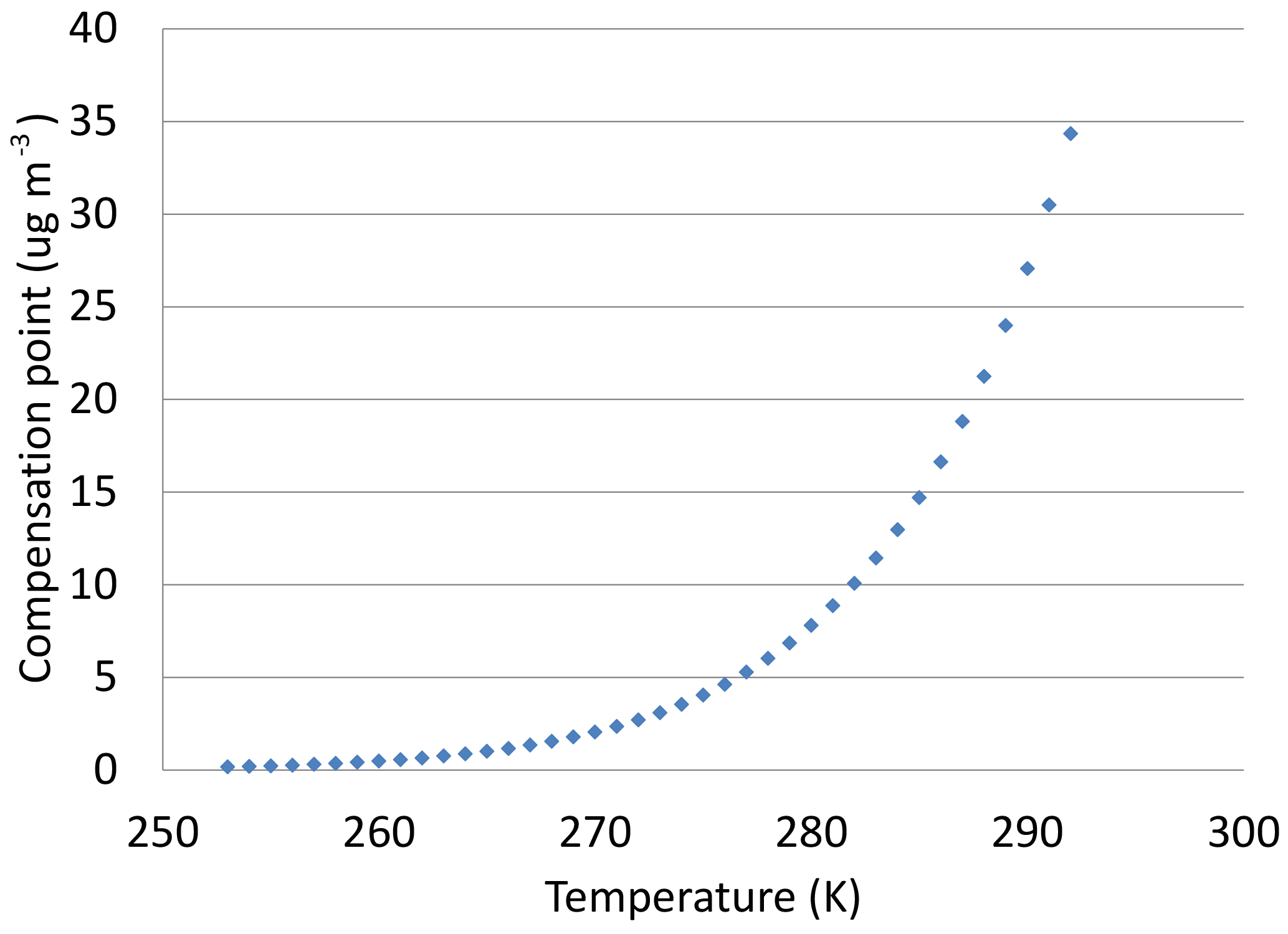
Figure 1Compensation point (Cg) relationship to temperature; Cg for evergreen needleleaf LUC shown as example.
Other chemical transport models, such as GEOS-Chem and CMAQ, use a similar method as Zhang et al. (2010); however, instead of the constant average soil emission potentials used here, they utilize a CMAQ–agroecosystem coupled simulation to calculate a soil pool from which to estimate Γg (Bash et al., 2013; Pleim et al., 2013; Zhu et al., 2015). In this case, the emission potential will vary and can go to zero if the NH in the pool is depleted. However, it was shown in Wen et al. (2014) that their Γst,g worked well during the same time of year as this investigation (August and September). This time of year was also shown in Zhu et al. (2015) to not have a large effect on emissions from the NH pool. Additionally, Wentworth et al. (2014) calculated the approximate relative abundances of NHx in the boundary layer versus NH in the soil pool to assess whether surface-to-air fluxes were sustainable. They found that soil NH concentrations were much greater than boundary layer NHx (by over 2 orders of magnitude), further supporting the assumption made here. In addition, the turnover time for soil NH is on the order of 1 day, hence it is unlikely that NH3 bidirectional fluxes would significantly deplete or enhance soil NH pools. Finally, given that GEM-MACH is used for real-time air quality forecasts at ECCC, it is not desirable for our bidirectional flux scheme to have to rely in advance on another model's output. Therefore, we use this simplified version, and assess whether its results provide an improvement (smaller biases and better correlations to measurements) to simulated NH3.
2.3 Addition of forest fire emissions
Our third model scenario (called “fire + bidi” hereafter) uses the GEM-MACH-Bidi model, and the exact same area emissions and anthropogenic major point emissions as the base and bidi scenarios. However, in addition, we add hourly North American forest fire emissions for all species to the major point emissions. The forest fire emissions system for GEM-MACH (called “FireWork is described in detail in Pavlovic et al. (2016). Briefly, to calculate the fire emissions for input to FireWork, biomass burning areas are first identified in near-real-time by the Canadian Wildland Fire Information System (CWFIS), which is operated by the Canadian Forest Service (http://cwfis.cfs.nrcan.gc.ca/home). CWFIS uses fire hotspots detected by NASA's Moderate Resolution Imaging Spectroradiometer (MODIS) and NOAA's Advanced Very High Resolution Radiometer and Visible Infrared Imaging Radiometer Suite imagery as inputs. Daily total emissions per hotspot are then estimated by the Fire Emission Production Simulator module of the BlueSky modelling framework (Larkin et al., 2009). SMOKE was then used to prepare model-ready hourly emissions of several species (including NH3) in a point-source format for model input.
In ECCC's operational forest fire forecasts, these emissions are used at 10 km resolution for the domain encompassing North America, with forest fires being treated as point sources with specific plume rise (Pavlovic et al., 2016). We have added 2013 forest fire emissions which were originally created for the 2013 FireWork forecasts to the anthropogenic point-source emissions used in the base case simulation, and have modified the GEM-MACH model to be able to accommodate the changing number of major point sources each day (as the number of fires changes daily). Fire plume rise is an ongoing area of investigation (e.g., Heilman et al., 2014; Paugam et al., 2016); smoldering emissions tend to be emitted directly at the surface, whereas flaming emissions can inject plumes to the upper troposphere. Here, we have set all fire emissions to be distributed evenly throughout the boundary layer, which is a simplification but one that averages out smouldering and flaming plume heights. Different parameterizations of fire plume rise are currently under development in GEM-MACH. The FireWork fire emissions are described in detail in Zhang et al. (2018), and this study represents the first time they have been used at a 2.5 km horizontal resolution.
2.4 Model setup for three scenarios
The base, bidi, and fire + bidi models were all run in the following way: each scenario was run from 1 August to 7 September 2013, where the first 11 days were “spin up” in order to allow chemical concentrations to stabilize, and are not used in our evaluation. This is a sufficient amount of spinup time, given that the atmospheric lifetime of NH3 is typically up to 1 day (Seinfeld and Pandis, 1998; Aneja et al., 2001), and given that it is close to the transport time of air crossing the larger North American domain. The time period from 12 August to 7 September was chosen to coincide with the intensive measurement campaign described in Sect. 3.
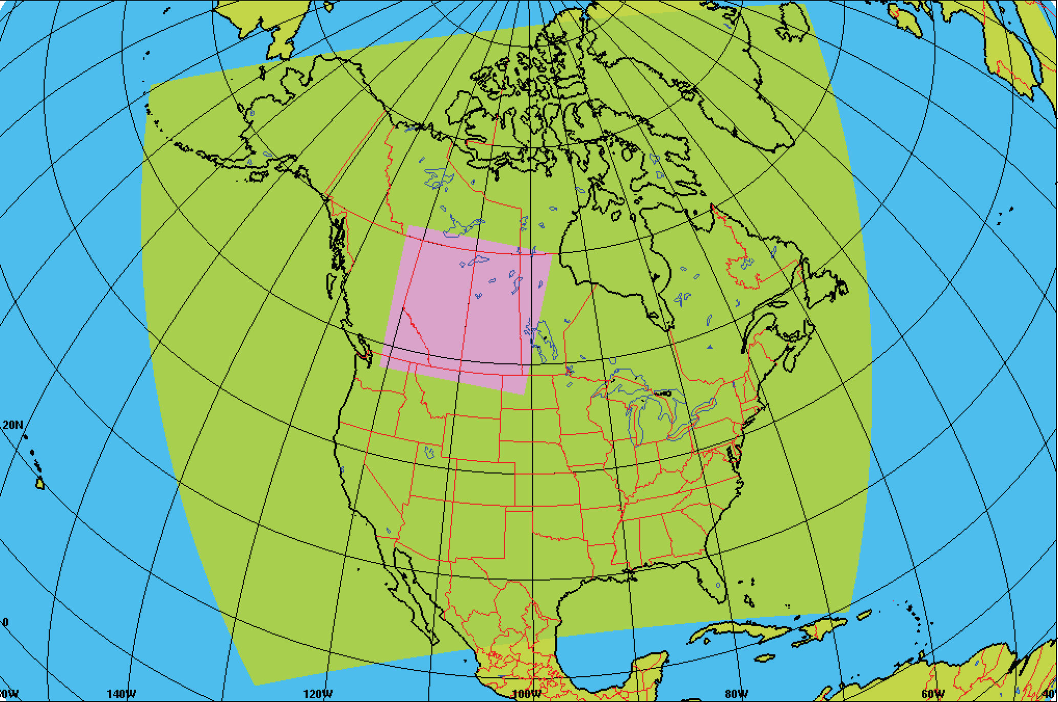
Figure 2Map of 10 km resolution continental piloting model domain (green) and 2.5 km resolution nested model domain (purple).
The model was run in a nested setup, whereby the North American domain was run at 10 km resolution using “climatological” chemical initial and boundary conditions from a 1-year MOZART simulation for all pollutants (Giordano et al., 2015). The nested oil sands region (which covers most of Alberta and Saskatchewan) was run at 2.5 km horizontal resolution, using the initial and boundary conditions from the 10 km North American model run. Figure 2 shows the two model domains.
The model simulations for the pilot and nested domains were not run as a continuous multi-day forecast but rather following the operational air quality forecast process, where the meteorological values are updated regularly with new analyses (products of meteorological data assimilation which provide optimized initial conditions for the 12 UTC hour of each day). The analyses were obtained from ECCC archives (Buehner et al., 2013, 2015; Caron et al., 2015), in order to prevent chaotic drift of the model meteorology from observations. Consequently, our simulation setup comprises simulations on the North American domain in 30 h cycles starting at 12:00 UTC, and the oil sands domain in 24 h cycles starting at 18:00 UTC (the 6 h lag being required to allow meteorological spinup of the lower resolution model). The next cycle uses the chemical mass mixing ratios from the end of the last cycle as initial conditions for the next 24–30 h. This system of staggered meteorological driving forecasts with a continuous chemical record continues until the full time period completes.
We run GEM-MACH in the 2-bin particle mode, which means that particles fall in either fine mode (diameter 0–2.5 µm) or coarse mode (diameter 2.5–10 µm), for computational efficiency (although sub-binning is used in some particle microphysics processes in order to ensure an accurate representation of particle microphysics; Moran et al., 2010), and in order to follow the setup used for the operational 10 km resolution GEM-MACH forecast.
Our three model simulations (base, bidi, and fire + bidi) are evaluated with surface, aircraft, and Cross-track Infrared Sounder (CrIS) satellite measurements. We briefly describe each of these observation datasets below.
3.1 AMS13 ground measurements
An extensive suite of instrumentation was deployed at monitoring site AMS13 (57.1492∘ N, 111.6422∘ W; 270 m a.s.l.; Fig. 3) from 7 August 2013 until 12 September 2013. Mining operations and bitumen upgrading facilities are 5 km to the south and north of the site, which is surrounded by boreal forest with dominant winds from the west averaging 1.9 m s−1 throughout the year. The average temperatures in the region for August are highs between 20–25 ∘C and lows around 10 ∘C, which is warm enough to make upward NH3 flux more likely (recall Fig. 1). However, temperatures drop rapidly at the end of August, into September, where the September highs average around 15 ∘C and lows around 5 ∘C. The skies are the clearest during August, with at least partly clear skies 50 % of the time. That said, the warm season (May through September) is the wetter season (average of 20 % chance of precipitation daily), with more precipitation than during the cold season (when there is an average of 7 % chance of precipitation daily). However, year-round precipitation, as well as relative humidity, are both relatively low in the AOSR. During the cold season (November through February), the average temperatures range from −21 to −5 ∘C, when the forest and soils are more likely to be a deposition sink for NH3. During November to April, it is also much cloudier, with February having cloudy conditions 77 % of the time. (All weather data cited here are from the annual report at Fort McMurray: https://weatherspark.com/y/2795/Average-Weather-in-Fort-McMurray-Canada-Year-Round).

Figure 3Flight path on 13 August 2013, where elevation (in metres) is denoted by the colour scale and the AMS13 site is indicated by a black circle.
NH3, fine particulate ammonium and nitrate, and other species were measured by an ambient ion monitor ion chromatograph via an inlet 4.55 m off the ground. The uncertainty of these measurements is ±15 %. These measurements are described in more detail in Markovic et al. (2012).
Data gaps sometimes appeared in the surface NH3 time series for the following reasons: instrument zero (14–15 and 17–18 August), instrument maintenance (19 August), and a power outage (27–28 August).
3.2 Aircraft measurements
During the oil sands monitoring intensive campaign, there were a total of 22 flights spanning 13 August to 7 September 2013. These measurements are described in detail in Shephard et al. (2015); Gordon et al. (2015); Liggio et al. (2016); and Li et al. (2017), and are summarized here. Aircraft NH3 measurements were conducted with a dual quantum cascade laser (QCL) trace gas monitor (Aerodyne Inc., Billerica, MA, USA; McManus et al., 2008), collecting data every 1 s. Outside air was sampled through a heated Teflon inlet tube shared with a high-resolution time-of-flight chemical ionization mass spectrometer (HR-ToF-CIMS); the flow rate through the QCL was 10.8 L min−1. The 1σ uncertainty for each measurement was estimated to be ±0.3 ppbv (±35 %; Shephard et al., 2015).
Particulate NH (0 to <1 µm in diameter) was measured by the Aerodyne high-resolution time-of-flight aerosol mass spectrometer (HR-ToF-AMS) instrument on board the same flights, which collected data every 10 s. The ambient air was drawn through a forward-facing shrouded isokinetic particle inlet from which the HR-ToF-AMS sub-sampled. The total residence time in the inlet and associated tubing was approximately 1 s. The error on these measurements is ±9 %. (Liggio et al., 2016)
Figure 3 shows a sample flight path from the campaign from 13 August 2013 – one of the 13 flights with valid NH3 measurements. The others took place on 15–17, 19 (two this day), 22–24, 26, 28 August, and 5–6 September 2013. NH3 data on the other nine flights were invalidated due to instrument issues (those on 14, 20–21, 29, 31 August, and 2–4 September 2013), but were successful for the NH measurements.
3.3 CrIS satellite measurements
CrIS was launched in late October 2011 on board the Suomi NPP platform. CrIS follows a sun-synchronous orbit with a daytime overpass time at 13:30 LT (local time, ascending) and a night time equator overpass at 01:30 LT (descending). The instrument scans along a 2200 km swath using a 3 × 3 array of circular pixels with a diameter of 14 km at nadir for each pixel. The CrIS “fast physical retrieval” described by Shephard and Cady-Pereira (2015) is used to perform satellite profile retrievals of NH3 VMR given the infrared emission spectrum from the atmosphere. This retrieval uses an optimal estimation approach (Rogers, 2000) that provides the satellite vertical sensitivity (averaging kernels) and an estimate of the total errors (error covariance matrix).
We take the CrIS retrieved profile and match it up with the closest model profile in both distance and time, compute the distance between the CrIS pixel and model field for each time step, and then select the time step that best matches the satellite overpass time. Since the model time steps are every hour with a 10 km spatial resolution they are always matched up to better than half an hour, and within 5 km.
An older version of GEM-MACH (v1.5.1) has been compared to TES satellite and aircraft measurements of ammonia over the AOSR (Shephard et al., 2015). Simulations with that version of the model were shown to be biased low, by about −0.5 ppbv throughout the lower-tropospheric vertical profile. This represented a substantial deficit in the model predicted sources of NH3, prompting the current work. We now compare our three GEM-MACHv2 simulations (base, bidi, and fire + bidi) against surface point measurements at the measurement site near an oil sands facility (AMS13), aircraft measurements over the broader AOSR, and satellite measurements over the Alberta and Saskatchewan area. We will discuss which simulation agrees best with measurements and where there may still be room for additional model improvement.
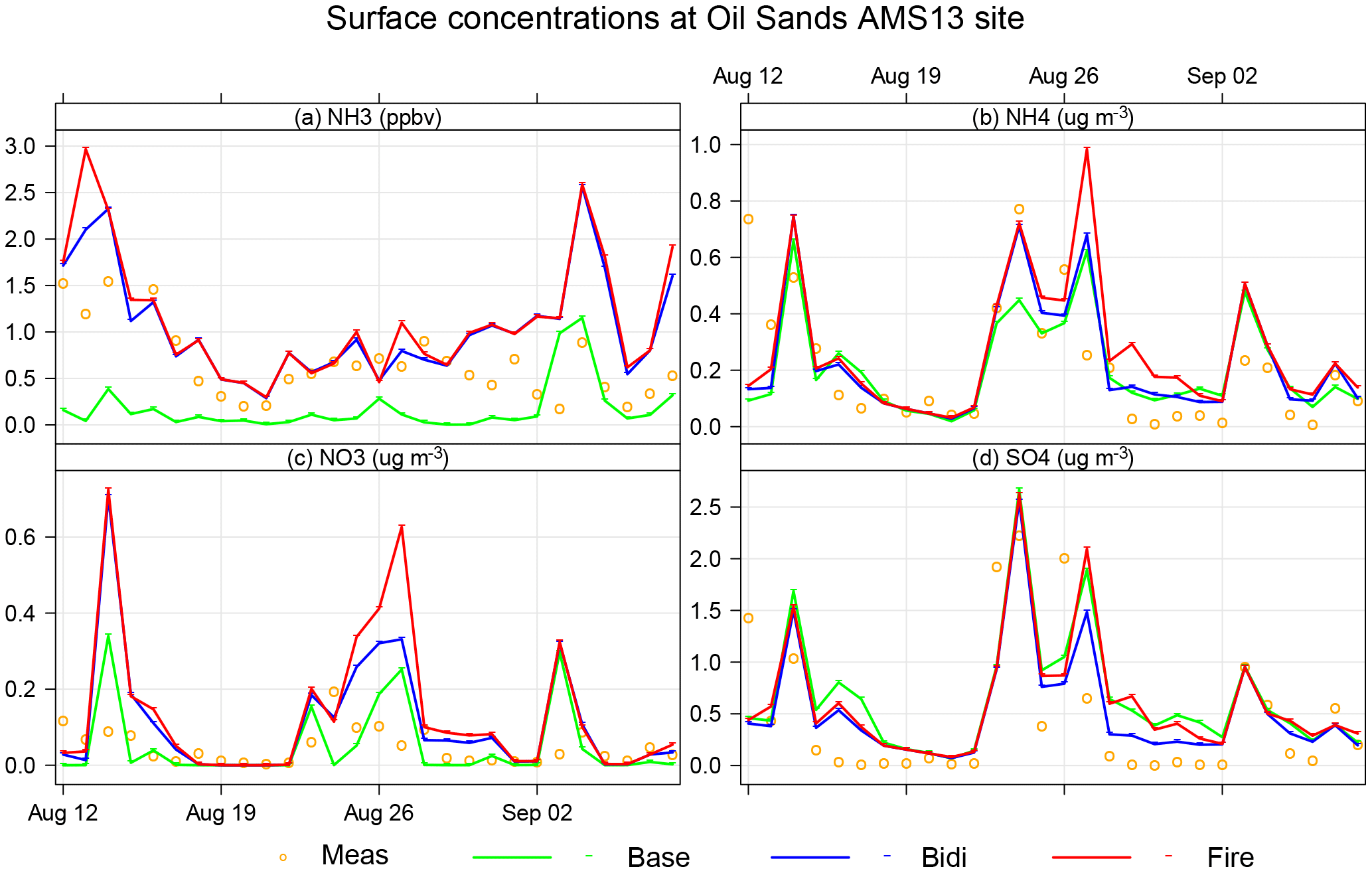
Figure 4Surface daily average VMR of (a) NH3, and concentrations of (b) fine particulate NH, (c) NO, and (d) SO at the AMS13 ground site in the AOSR. Measurements (Meas) in orange, base model in green, bidirectional flux model (Bidi) in blue, and fire + bidi model (Fire) in red.
4.1 At the AMS13 ground site
Figure 4 shows the time series of the daily average (for clarity) VMRs of NH3 and concentrations of fine-particulate NH, NO, and SO at the AMS13 oil sands ground site for the observations and three model simulations. The hourly data were also studied, but are not shown in the time series.
We first note that the NH3 VMRs in the measured time series are relatively low with mean, median, and maximum of 0.6, 0.426, and 2.98 ppbv, respectively, in the hourly data, which are lower than the 1–8 ppbv range in Bytnerowicz et al. (2010) and the 2.7 ppbv summertime mean given in Hsu and Clair (2015). However, this may be due to the different time periods and locations measured. Our mean measured values at the AMS13 site are similar to the VMRs found at U.S. AMoN background sites (http://nadp.sws.uiuc.edu/amon/).
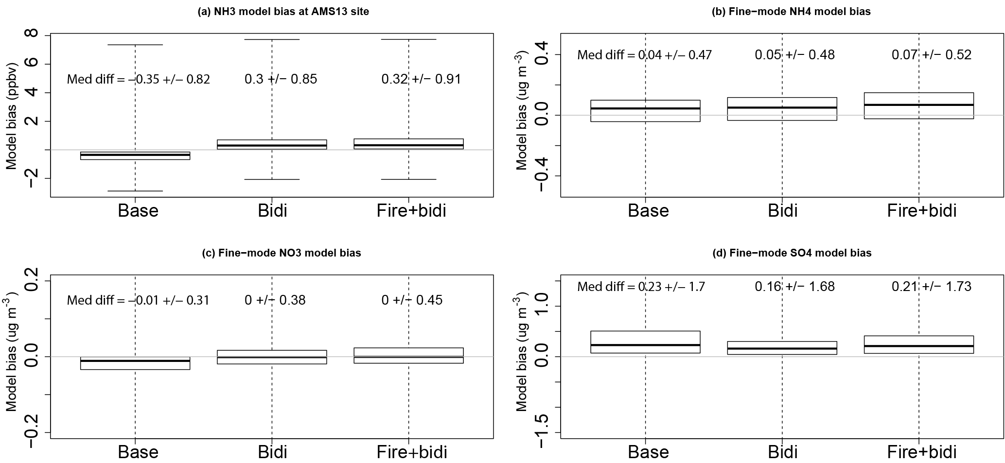
Figure 5Hourly model–measurement bias in surface (a) NH3 VMR, and (b) NH, (c) NO, and (d) SO concentrations at the AMS13 ground site in the AOSR.
Figure 4a shows that the base model (green) background VMRs of NH3 are very low (nearly 0 ppbv when there is no plume influence) compared to the measurements (orange). Only during the spike on 3–4 September does the base model exceed the measured values, probably indicating a local plume event fumigating to a lesser extent in the observations than was predicted by the model. The NH3 VMRs of the base case are biased low compared to the surface measurements by a median of −0.35 ppbv (Fig. 5a) over the time period of the campaign. In Fig. 4, the bidi model (blue line) and fire + bidi model (red line) show a significant improvement to the NH3 VMRs compared to the base model (green line). Unfortunately, during some time periods, these two versions of the model overestimate NH3: during 13 August, the model adds a significant level of NH3 due to fire emissions; however, the surface in situ observations show no evidence of fire impact. During other time periods (e.g., 30 August to 3 September, and 4–7 September), the bidi model appears to have put too much NH3 into the system. Therefore, the bidi model bias (Fig. 5a) is now 0.30 ppbv too high (median), and the fire + bidi bias is 0.32 ppbv high (median) over the time period of the campaign, resulting in an overall improvement of only 0.03 ppbv in the model bias.
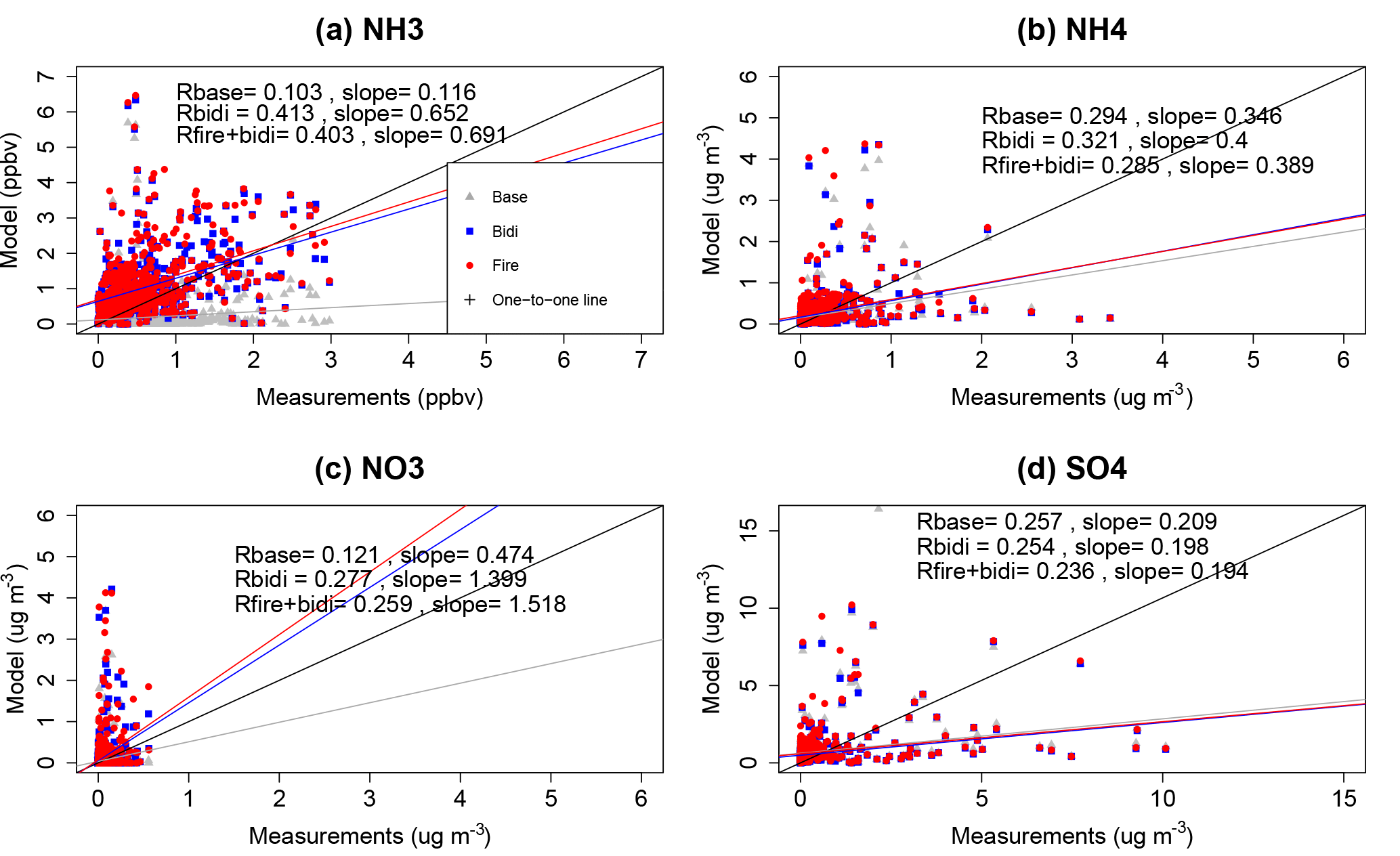
Figure 6Hourly modelled vs. measured surface (a) NH3 VMR, and (b) NH, (c) NO, and (d) SO concentrations at the AMS13 ground site in the AOSR. Base model is in grey, bidirectional flux model in blue, and fire + bidi model in red.
While the bias improvement is small, the bidi and fire + bidi both have greatly improved correlation coefficients (from R=0.1 to 0.4) and slopes much closer to 1 (from 0.1 to 0.7), showing that those added sources are important to improve model results (Fig. 6a). Additionally, the diurnal cycle (not shown) was improved in the bidi simulation, with both it and the measurements shaped like a sine curve with a minimum at 03:00–04:00 LT, and a maximum at noon local time, although the amplitude of the cycle was underestimated. Whereas, the base model diurnal cycle was flat from midnight to noon local time, and spiky from noon to midnight.
While Figs. 4a to 6a show that the addition of bidirectional flux improves the model correlation coefficient, slope, and bias, there is still room for further improvement. Paired t-test results indicate that the fire + bidi and measurements are still significantly different (see Table 2 for comparison statistics of all three simulations). While inherent limitations from model resolution and uncertainties may be responsible for the remaining bias, it is likely that (a) the emission potentials for the LUCs in the region may be causing too much re-emission of NH3, and need refinement, and (b) the fire emissions of NH3 are not properly distributed in the vertical, placing too much NH3 near the surface and/or the fire emission factors for NH3 are too high.
Refinement needed for the emission potentials and LUCs may be a significant cause of the bidi and fire + bidi model biases. Rooney et al. (2012) have shown that about 64 % of the AOSR are wetlands (fens, bogs, and marshes), which should be mapped to the swamp LUC. However, our model currently assigns the AOSR landscape to evergreen needleleaf trees, deciduous broadleaf trees, inland lake, mixed shrubs, and mixed forests (and none of the region to swamp). This would lead to an overestimation of re-emission given that bogs are fairly acidic and our swamp emission potential is lower than the aforementioned LUCs. Other evidence for these two explanations will be presented below in Sect. 4.3.
For NH, NO and SO the time series, model biases, and model-vs.-measured correlations are shown in Figs. 4, 5, and 6, respectively. There is very little change in NH (Figs. 4b, 5b, and 6b) and SO (Figs. 4d, 5d, and 6d) despite the increase in NH3 that the bidirectional flux yields. The bias is very small for all three model scenarios, and the correlation coefficients are all relatively poor. So while there is an improvement to modelled NH3 with bidirectional flux, there is a neutral affect on fine particulate NH. This may be because the charge of NH in the particles is already enough in the base model to balance the charge of 2 × SO NO in the aerosols, thus causing any additional NH3 (from bidi and fires) to remain in the gas phase. Alternatively, the minimal change in NH could be due to additional wet scavenging of the additional NH3, which will be discussed in Sect. 5.2. The change in NH3 VMR has no effect on SO since particulate SO is not sensitive to the amount of NH3∕NH available, and is dominated by anthropogenic and fire emissions. For NO (Fig. 5c), the base model bias was quite small at 0.01 µg m−3; however, the addition of bidi and fire + bidi further reduced that bias to 0.0011 and 0.0004 µg m−3, respectively, which is a significant improvement. The correlation coefficient for NO also improved from about 0.1 to 0.3 (Fig. 6c).
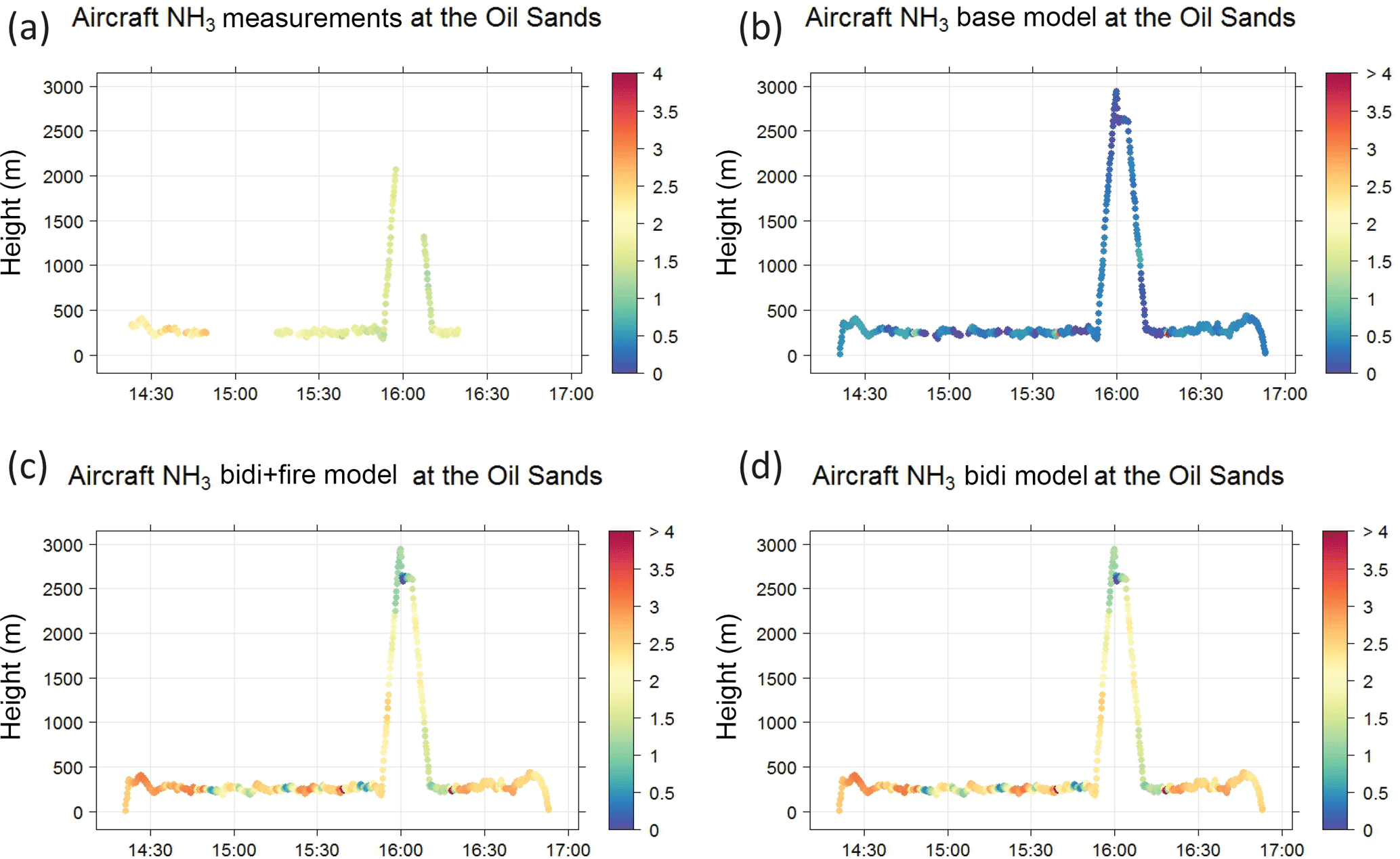
Figure 7NH3 VMRs aloft (colour scale) over the oil sands region during the 13 August 2013 flight. (a) Measurements, (b) base model, (c) fire + bidi model, and (d) bidi model.
4.2 Along the oil sands campaign flight paths
There were 13 flights during the oil sands campaign that had valid (above detection limit, and no instrument error) NH3 measurements, and 22 flights that had valid NH (0–1 µm diameter) measurements. The flight path of the first flight, which occurred on 13 August 2013, is shown in Fig. 3; chosen as an example because this flight sampled mainly background NH3 (rather than facility plumes).
Figure 7 shows the NH3 VMRs along this flight path over time. Here the hourly model output is interpolated to the same time frequency as the measurements. The model output also has spatial resolution limits when comparing to the aircraft. However, we clearly see that for this flight, the bidirectional flux has increased NH3 VMRs, bringing them closer to the measured values (median biases for this flight are −1.38, 0.68, and 0.69 ppbv in the base, bidi, and fire + bidi simulations, respectively). There is little change when fires are added (Fig. 7d vs. c) because this flight did not pass through a fire plume.
Figure 8Hourly averages along all flight paths over the oil sands region during the summer 2013 campaign: model–measurement bias in (a) NH3 and (b) NH. Modelled vs. measured (c) NH3 VMR and (d) NH concentrations aloft. Base model is in grey, bidirectional flux model in blue, and fire + bidi model in red.
Figure 8 shows the model–measurement differences and the model vs. measurement scatter plots for the combined set of all flight paths for hourly average NH3 and NH. For NH3 the median base model bias is −0.75 ppbv, comparable to the bias observed in Shephard et al., 2015, with the bidi model bias improving to −0.24 ppbv and the fire + bidi bias improving to −0.23 ppbv. Also, the best correlation coefficient and slope is achieved by the fire + bidi scenario. The use of the bidirectional flux has thus reduced the model bias relative to the aircraft observations by a factor of 3. The fire + bidi simulation has the best statistics compared to measurements, as summarized in Table 2.
Again, the NH results show little change despite the increase in NH3. The small bias from the base case gets insignificantly smaller, and the slope and correlation coefficients are all negligibly changed.
4.3 In the vertical profiles across the region
The CrIS satellite has many observations over North America during the 2013 oil sands campaign. We have evaluated the model with these observations in two ways:
-
All daytime data from 12 August–7 September 2013, with model–measurement comparisons over a large region encompassing Alberta and Saskatchewan (latitude range: 48–60∘ N, longitude range: 100–122∘ W), which contains agricultural areas, a number of cities, the northern boreal forest, and oil sand facilities.
-
Case studies where we attempt to isolate fire emissions and non-fire conditions to evaluate both new components (fires and bidi) of the model.
The latitude and longitude ranges of our model–measurement pairs are given in Table 1. The satellite passes over these regions at approximately 13:00 LT and 01:00 LT.
Table 1Latitude and longitude ranges that the model was evaluated over with the CrIS satellite measurements.
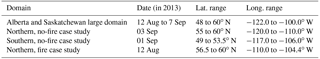
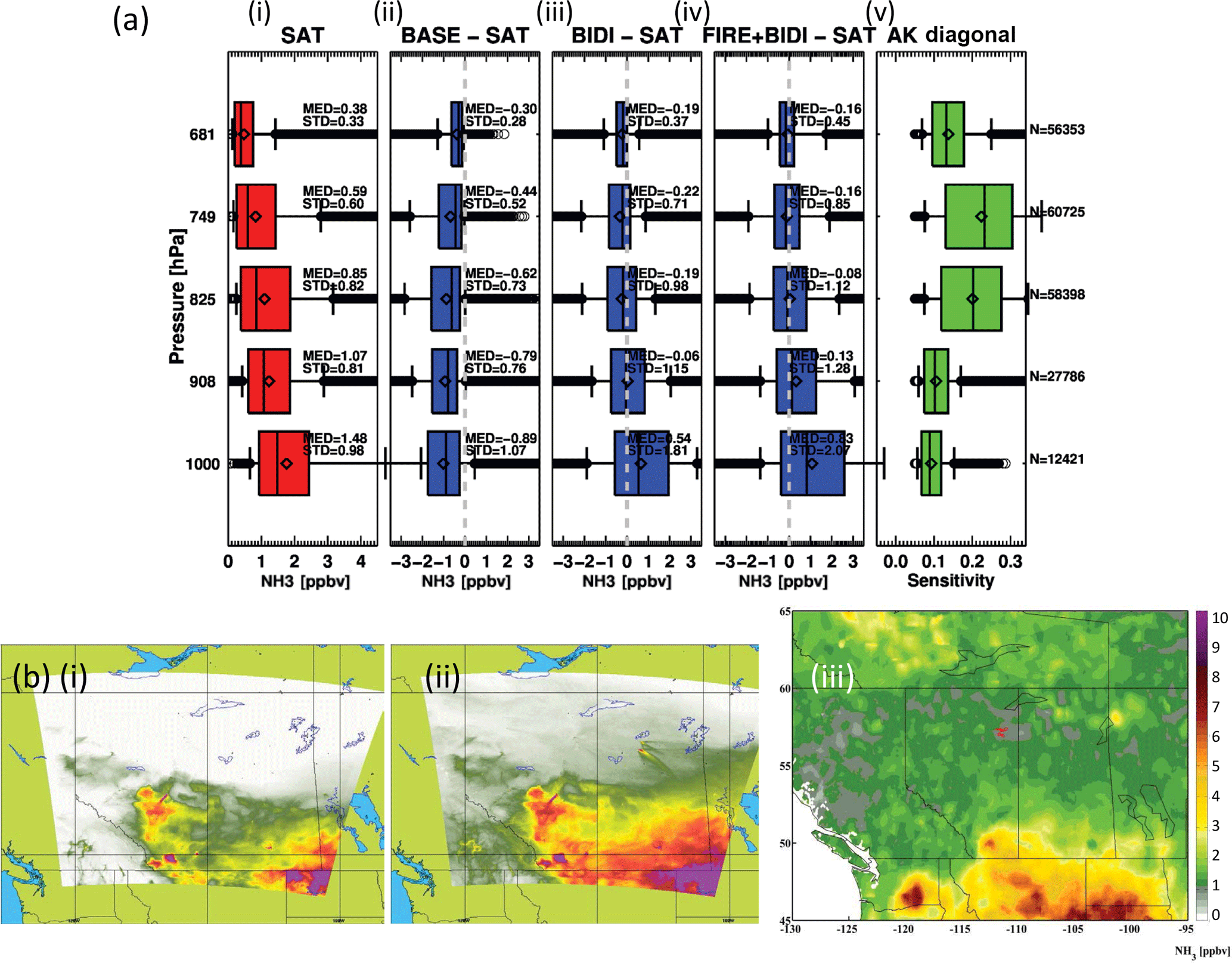
Figure 9(a) (i) NH3 vertical profiles as measured by CrIS satellite from 12 August to 7 September 2013; difference between measurement and (ii) base model, (iii) bidi model, and (iv) fire + bidi model; and (v) averaging kernel (labelled AK) of CrIS satellite for NH3 retrieval. (b) Average (12 August–7 September 2013) surface NH3 VMRs given by the (i) base model, (ii) fire + bidi model, and (iii) CrIS satellite.
There were over 60 000 model–measurement pairs between the model and the CrIS satellite over the model domain during 12 August to 7 September 2013. Figure 9a presents model biases for the entire dataset in a box and whiskers plot of the vertical NH3 profiles at five vertical levels. The left-most panel (panel i) shows the NH3 VMRs measured by CrIS, and the right-most panel (v) shows the diagonal elements of the CrIS averaging kernels, illustrating the sensitivity of the satellite measurements to each vertical level. The NH3 VMRs over Alberta and Saskatchewan measured by CrIS are very similar to those found by TES in the Shephard et al. (2015) study for the AOSR region.
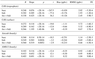
The middle panels (Fig. 9a, ii–iv) show the model biases from the three simulations. The base model has a very similar bias to CrIS as the older version of GEM-MACH (v.1.5.1) had compared to TES observations in the Shephard et al. (2015) study – thus showing that the negative NH3 biases were not improved with the use of the newer GEM-MACH version (v2) itself. The fire + bidi model has the smallest bias in the highest three layers, but the bidi model has the smallest bias in the two lowest layers. In those lower layers, the fire + bidi model increases NH3 VMRs too far (though still a smaller absolute bias compared to the base case; Fig. 9a). The fire + bidi positive bias could be due to an overestimate of the bidirectional flux re-emissions or of the fire emissions, or to an underestimate of the altitude of the fire emissions, or a combination of all three factors. In order to distinguish between these possibilities, two case studies were examined further in the next section. The statistics from the model–CrIS comparison can be found in Table 2. That summary shows that the fire + bidi simulation performs better than the base and the bidi simulations.
The spatial distribution of modelled NH3 can also be evaluated with CrIS measurements, as shown in Fig. 9b. These are maps of the average surface NH3 from the base model, the fire + bidi model, and the CrIS satellite. The fire + bidi model over-predicts the effect of fires in the middle of northern Saskatchewan, but appears to be missing fires in north-western Manitoba. Other than fire influence, the spatial distribution in the fire + bidi model is the same as that of the base model, but with significant increases in overall VMR. The spatial distribution of the model simulations is different from the spatial distribution that CrIS measures. For example, the model predicts much higher NH3 near the city of Edmonton than CrIS shows. That said, the addition of bidirectional flux has greatly improved the NH3 simulation in the northern part of the province, where it was almost zero in the base model.
Table 2Model–measurement NH3 comparison statistics from 12 August to 7 September 2013: R is correlation coefficient; slope is of the line-of-best-fit between model vs. measurement; p and t are from a paired t test between model and measurement data pairs (p> 0.05 and means that the model is statistically indistinguishable from measurements); the median model bias; RMSE is the root mean square error; and FE is the fractional error of the models. CrIS (troposphere) results are for the entire model domain at all tropospheric levels shown in Fig. 9(top), and CrIS (surface) results are for the lowest retrieval level (both are during mid-day satellite overpass times); aircraft results are from the 12 flight paths over the oil sand facilities, hourly averages during the daytime; and AMS13 results are from hourly data (day and night) at the one ground station.
We selected three sample days (12 August and 1 and 3 September 2013) that we use for the case studies. The measured surface NH3 and sample Aqua MODIS true colour composite maps for those days are shown (Fig. 10). The four boxed regions on those maps indicate where model–measurement pairs were sampled for this study. The cyan and black boxes (in Fig. 10a and b) are the regions where we sample clear-sky and no-fire conditions on 3 and 1 September 2013, respectively. The magenta box in Fig. 10c is the region where we isolated our fire case study on 12 August 2013. The blue box is the region we discussed above, which we analysed for the full time period simulated (12 August–7 September 2013; Fig. 9a).
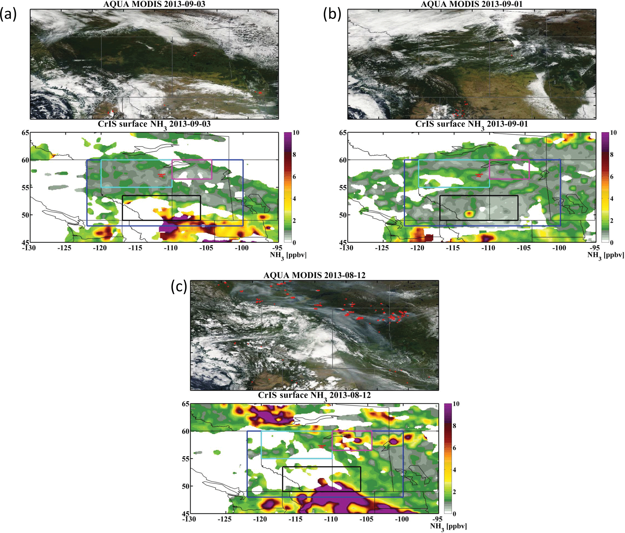
Figure 10Images of the Alberta and Saskatchewan region with clouds and fire hotspots from MODIS (upper panels). Maps of CrIS-measured surface NH3 VMRs, with coloured boxes showing the regions where model and satellite measurements were sampled (lower panels). These three examples are for (a) northern bidi case study (cyan), (b) southern bidi case study (black), and (c) fire case study (magenta), discussed in Sect. 4.3, and the blue box is the region of our overall comparison.
4.3.1 Case study 1: clear-sky days with little fire influence – evaluating bidi
In order to evaluate the bidirectional flux component separately from the fire component, we selected 3 September (northern, boreal forest and AOSR region – cyan box in Fig. 10a) and 1 September (southern, agricultural region – black box in Fig. 10b), where the MODIS maps (EOSDIS NASA Worldview map; https://worldview.earthdata.nasa.gov/) showed very little hotspots from fires and conditions that were relatively cloud and smoke free, which yield the most CrIS observations (see Table 1 for the latitude and longitude ranges). Figure 10 also shows the surface NH3 VMRs as observed by CrIS on each of those days. Figure 11a shows that in the north, the bidi model improves the bias from −0.84 to −0.07 ppbv in the lowest vertical level, and smaller, but still significant, improvements to the bias at the other levels. The fire + bidi model has a nearly identical impact as the bidi model, which is expected in a fire-free zone. Therefore, the GEM-MACH-Bidi model performs very well in northern Alberta and Saskatchewan where there is mainly boreal forest, and background-level NH3. This also implies that the LUC assignment discussed in Sect. 4.1 may only apply to a small region around the AOSR, and not to the overall large region we have defined here.
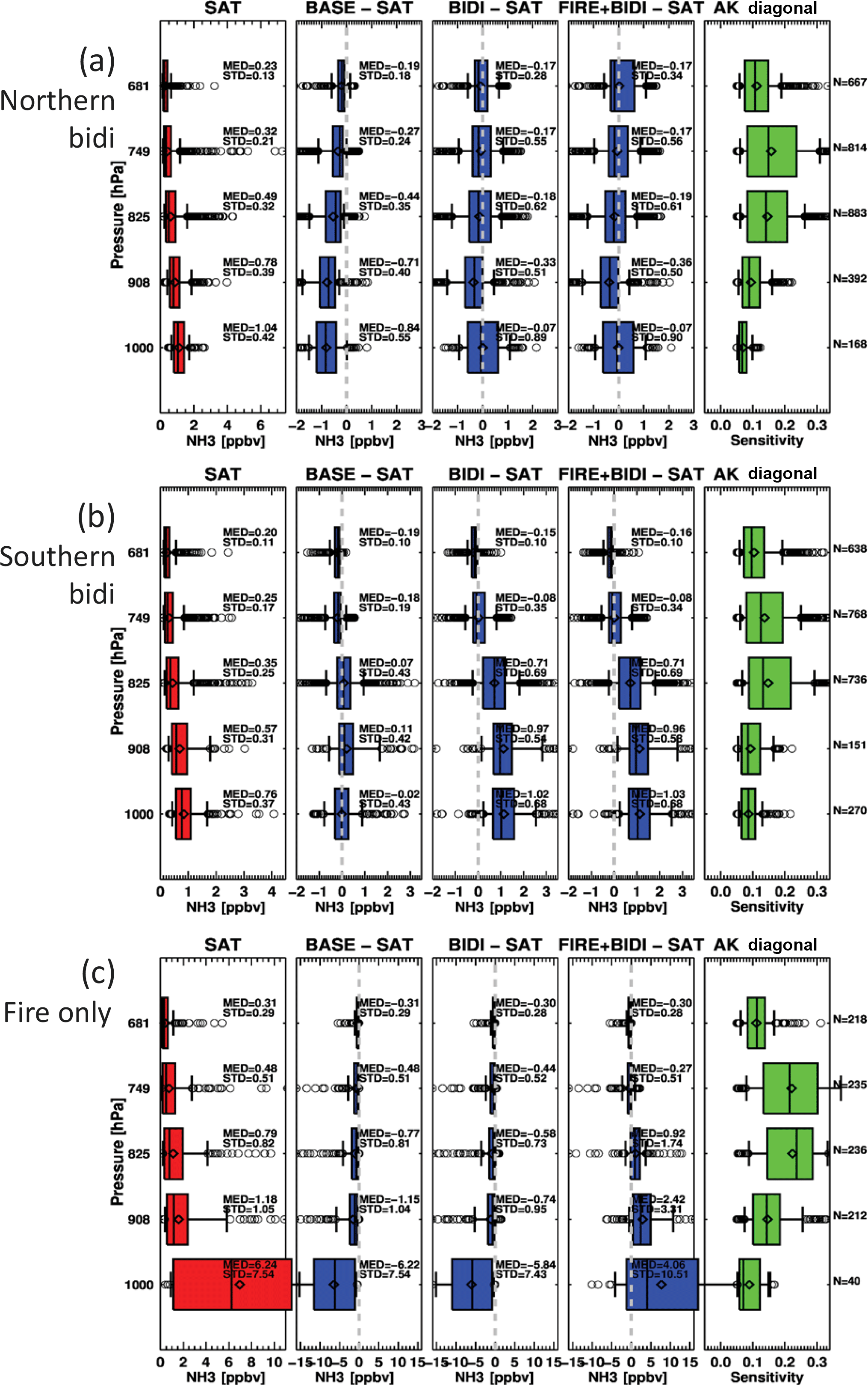
Figure 11As in Fig. 9a, but for our (a) northern “bidi-only” case study (3 September 2013), (b) southern “bidi-only” case study (1 September 2013), and (c) northern “fire-only” case study (12 August 2013). These regions are shown in Fig. 10a (cyan), 10b (black), and 10c (magenta) boxes, respectively.
In the southern region (Fig. 11b), the addition of bidirectional flux moves the bias from near-zero to +1.02 ppbv in the lowest level. In this case, the base model with no bidirectional flux appears to be the most accurate model in areas dominated by agricultural sources. There are two possible explanations: (a) agricultural emissions are too high in the base model, and the addition of the bidirectional flux leads to an overestimation of the NH3 amounts or (b) re-emissions from bidirectional flux from crops are not significant. The literature (Bash et al., 2010; Massad et al., 2010; Zhang et al., 2010; Zhu et al., 2015) indicates that crops do indeed re-emit NH3, therefore (a) is the more likely explanation. The agriculture NH3 emission inventory we used was created by the NAESI (National Agri-Environmental Standards Initiative) project (Bittman et al., 2008; Ayres et al., 2009; Makar et al., 2009) and has about 30–200 % uncertainty associated with it (Bouwman et al., 1997; Asman et al., 1998). Therefore, with improved national NH3 emission inventories, GEM-MACH-Bidi is likely to improve model results across the domain.
4.3.2 Case study 2: a clear-sky day with significant fire influence – evaluating fires
In order to evaluate the fire component separately from the bidirectional flux, we selected 12 August (a northern region with little-to-no agricultural contributions) where the MODIS map shows numerous hotspots from fires and smokey conditions (Fig. 10c; magenta box). The base and bidi models underestimate NH3 VMRs (Fig. 11c) by −6.22 and −5.84 ppbv, respectively (in the lowest vertical layer), but the fire + bidi model overestimates NH3 by +4.06 ppbv. The fire + bidi version of the model still has the lowest bias of the three simulations; however, either (a) the fire + bidi model does not distribute the fire emissions properly in the vertical, (b) the fire emissions of NH3 are too high, or (c) the model's oxidation rate of NO2 and SO2 in the fire may be underestimated, resulting in less sulfate and nitrate to convert NH3 to NH. It is potentially a combination of all three explanations, as both fire-plume rise and fire emission factors are ongoing areas of study, and we further elaborate below.
Shinozuka et al. (2011) suggest that fire plumes are Gaussian-distributed in a thin layer aloft, which is not how our current fire-emissions module distributes the fire plume. In our simulation, the fire emissions are distributed evenly throughout the boundary layer (the first 3–4 layers in Fig. 11c). However, we do not believe our parameterization of plume distribution causes the fire + bidi bias since the positive bias extends throughout the first three vertical layers and does not go negative in any layer (Fig. 11c), as would be expected if mass redistribution of the plume was the cause of the biases. We also know that the plume heights for most of the Fort McMurray fires of 2016 reached only up to 3–4 km altitude range based on the NASA Cloud-Aerosol Lidar and Infrared Pathfinder Satellite Observation (CALIPSO) and Multi-angle Imaging Spectroradiometer (MISR) satellite observations. Therefore, the fire plumes are not located above the altitudes we studied.
Unfortunately, there were no flights that captured the fine structure of the fire plumes during the 2013 monitoring intensive campaign that can be used to further corroborate the vertical distribution of the fire plumes. There will, however, be flight observations of fires during the planned 2018 AOSR measurement campaign.
Explanation (b) seems the most likely, as the uncertainty in emission factors for NH3 from wildfires is very large (e.g., ±50–100 % depending on the fuel type; Urbanski, 2014), and could easily be overestimated. The NOx and SO2 fire emission factors have smaller uncertainties of ±10–40 % (Urbanski, 2014). Therefore, the model may be further improved with reduced NH3 emission factors for fires.
5.1 Effect on ambient ammonia
Given that the overall fire + bidi model agrees best with measurements in the greater Alberta/Saskatchewan region (discussed throughout Sect. 4, and Table 2) and contains all known missing sources of NH3, we can use the model to answer one of our key questions: what percent contributions to total ambient NH3 VMRs came from bidirectional flux versus from forest fires during the study time period? We do so by subtracting the bidi model output from the fire + bidi model output to get the forest fire component, and subtracting the base model output from the bidi model output to get the bidi component. The absolute differences are calculated as follows:
which tell us how many ppbv of NH3 on average is associated with re-emissions of NH3 (upward component of bidirectional flux) versus fire emissions.
The percent differences are calculated as follows:
which tell us what percent of total NH3 VMRs on average comes from re-emissions of NH3 and from fire emissions, assuming the NH3 from our fire + bidi simulation is the true total NH3.
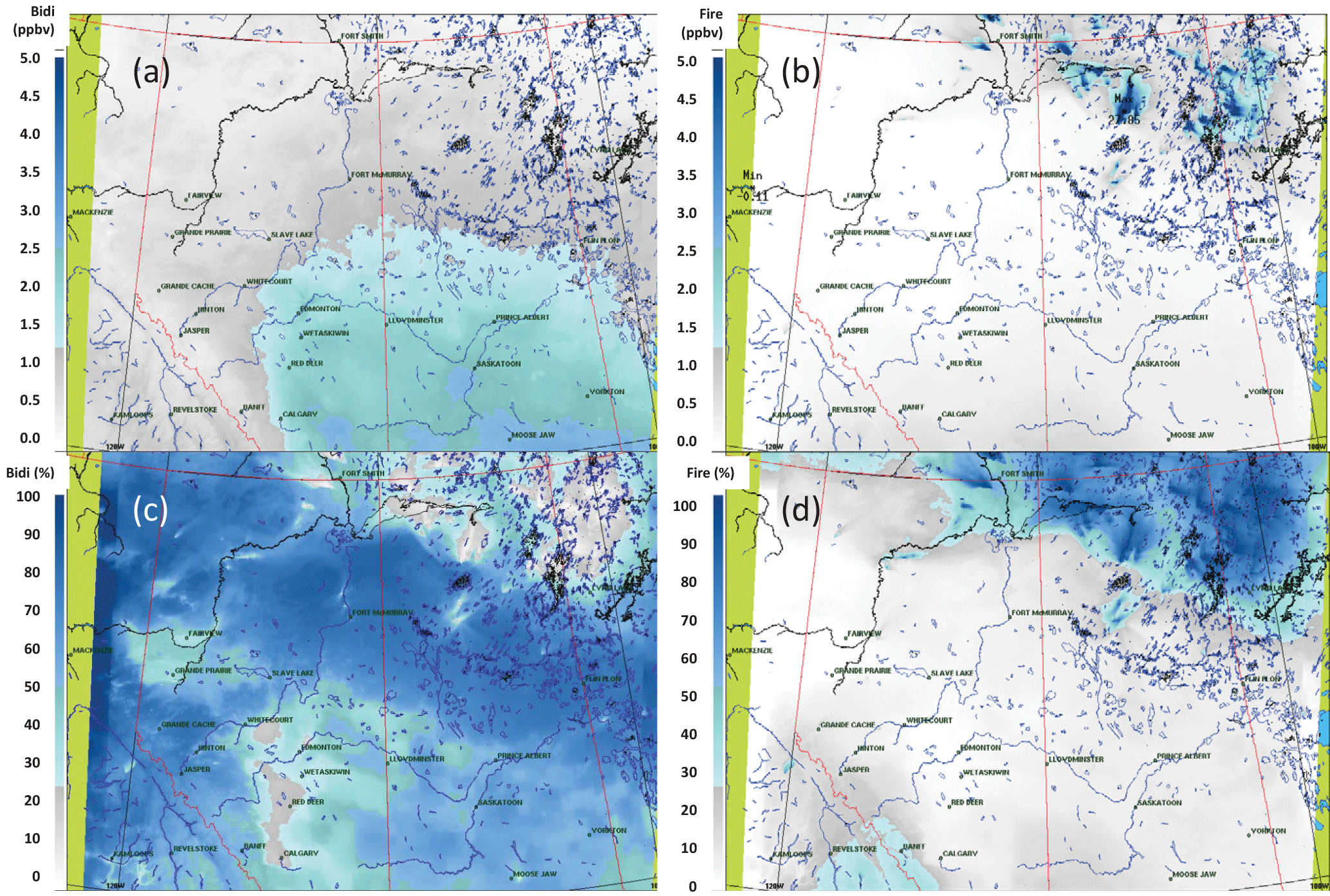
Figure 12Maps of the modelled (a) absolute bidirectional flux contribution, (b) absolute fire contribution, (c) percent bidirectional flux contribution, and (d) percent fire contribution to surface NH3. These are averages over 12 August to 7 September 2013.
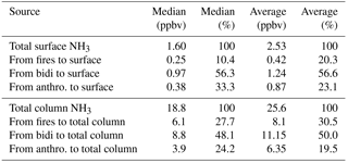
We perform this calculation on the averaged model output (12 August to 7 September 2013) over the 2.5 km model domain, and get an average of 20.3 % (or 0.42 ppbv) and a median of 10.4 % for ambient surface NH3 VMRs that come from forest fires (Fig. 12b and d). The mean and median are so different because fires are sporadic, large contributions to NH3 VMRs, and the mean value is more sensitive to the big outliers. We get an average of 56.6 % (or 1.24 ppbv) from bidirectional flux (56.3 % median; Fig. 12a and c), and the remaining 23.1 % average (33.3 % median) comes from direct emissions from anthropogenic sources (agriculture, fossil fuel combustion, oil sands industry, etc.). These numbers are summarized in Table 3. The increase in NH3 due to the bidirectional flux scheme is of the same order of magnitude as that found in the Zhu et al. (2015) study using the GEOS-Chem model, during the month of July in the United States (where they found ∼1 ppbv increase in surface VMRs due to bidirectional flux). It is also similar to values found in Europe in the Wichink Kruit et al. (2010) study.
Table 3Average source contributions to ambient NH3 VMRs over the Alberta and Saskatchewan model domain during 12 August to 7 September 2013.
Over the model domain, the minimum bidi influence on surface NH3 is just north of Edmonton, where only 1 % of NH3 comes from bidi. Similarly, two AOSR facilities north of Fort McMurray stand out as having small bidi influence (12–40 %, surrounded by values greater than 90 %; Fig. 12d). Also, any remote region with fire emissions will have a small percentage contribution from bidirectional flux during the fires, as they are in northern Saskatchewan (Fig. 12d). This is expected given that the average VMRs in cities and near large sources are very close to, or exceed, the compensation point. The absolute maximum in the bidi component map is 4.5 ppbv in the lower right corner (an agricultural region with high NH3 emissions), and the minimum is 0 ppbv (Fig. 12b). This means that nowhere in the domain did the bidirectional flux formula result in more net deposition than the base model calculated via the Welesley–Robichaud–Zhang scheme. The maximum fire contribution to surface NH3 is 27.9 ppbv where large fires occurred in northern Saskatchewan (Fig. 12c).
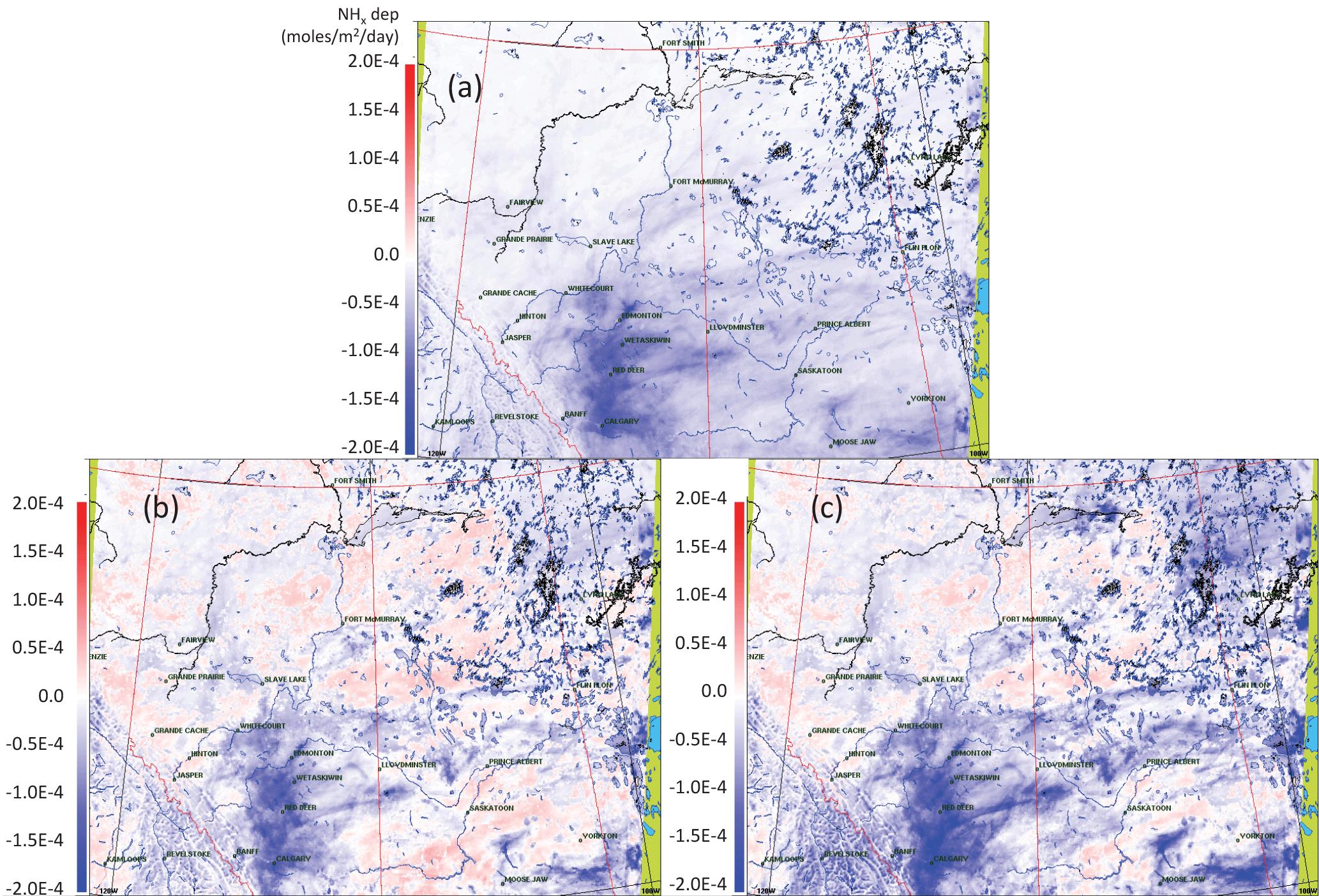
Figure 13Maps of the modelled average NHx deposition for (a) base, (b) bidi, and (c) fire + bidi models. In all maps, red/positive represents upward flux and blue/negative represents downward flux. These are daily amounts averaged over 12 August to 7 September 2013.
5.2 Effect on deposition
Similar to our analysis from the previous section, we can use the model to determine how bidirectional flux and fires impact daily NHx deposition (which equals the dry deposition of NH3 + the wet deposition of NH). Figure 13 shows the average daily net deposition (or net flux) of NHx from the base, bidi, and fire + bidi models. Negative (or blue) indicates net deposition (downward flux), and positive (or red) net emission (upward flux). The base model (Fig. 13a) had no re-emission (upward flux) option, thus NH3 was always net dry deposited in that scenario. The bidi (Fig. 13b) and fire + bidi (Fig. 13c) maps show that most of the Alberta and Saskatchewan area has net deposition (e.g., near the cities, agriculture, and forest fires), but that some regions (with low atmospheric NH3 VMRs) have net emission of NHx. The dry NH3 flux is net positive over the domain; however, when the increase in wet NH is accounted for, the net flux of NHx is still negative (downward). This is very similar to what Wichink Kruit et al. (2010) found in a 2007 study in Europe; a reduction in dry NH3 compensated by an increase in wet NH deposition.
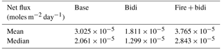
Note that the assumption of an infinite soil pool of NH in our bidirectional flux scheme has not caused an overwhelming upward flux of NHx. In fact, the average results across the domain actually have more deposition in the fire + bidi scenario than in our base scenario. Table 4 shows the mean and median net NHx flux for each scenario (presented as deposition, so negative signs removed). That said, following the soil pool approach (Pleim et al., 2013; Zhu et al., 2015), the soil pool of NH may eventually get depleted. However, we believe this to be very unlikely for the following reasons: (1) deposition of NHx throughout the year continually replenishes the soil pool – especially when temperatures are cooler in winter, spring, and fall since the compensation point is exponentially dependent on temperature. (2) The short time frame of this study would not be long enough to deplete the soil pool. For example, Zhu et al. (2015) needed to spin up their model for three months in order to get the NH4 soil pool stable, implying both a large pool and a long time required for it to empty.
Table 4Average NHx deposition (downward flux) over the Alberta and Saskatchewan model domain during 12 August to 7 September 2013.
In the AOSR near Fort McMurray, we can compare our NH3 dry deposition results to those calculated in Hsu et al. (2016). Their values for nitrogen range from 0.7 to 1.25 kg ha−1 yr−1 (or 1.13 to 2.01 × 10⁻⁵ moles m−2 day−1), while ours are 10 times lower at around 0.13 kg ha−1 yr−1 (scaled up to a year, from 2.12 × 10⁻⁶ moles m−2 day−1) near Fort McMurray, and do not vary much among our three model scenarios. These differences in deposition estimates are likely due to the fact that our study is only during a very warm time of the year, when deposition will be at a minimum, whereas the Hsu et al. (2016) study covered both winter and summer time periods for multiple years. The differences may also be partially due to the fact that our modelled ambient NH3 VMRs are also low compared to those measured in Hsu and Clair (2015) near Fort McMurray. They measured an average of 1.55 ± 0.6 ppbv (1.9 µg m−3) at Fort McMurray, whereas our fire + bidi model has an average of 1.01 ppbv there (0.73 ppbv in bidi, and 0.39 in base). There may also be differences in that our model has more of the NHx deposition coming down as NH rather than as NH3.
Our fire + bidi NHx deposition values (Table 4) are well in line with reported NH3 deposition in Kharol et al. (2017), who report satellite-derived NH3 deposition of about 2.1 to 7.0 × 10⁻⁵ moles m−2 day−1 in Alberta, and are at the low end of NH3 deposition values reported within Behera et al. (2013).
The difference in deposition between the fire + bidi and bidi cases – which is the contribution of fires to the total NHx flux – showed that the fires increased downward flux or deposition over large swaths of the domain (e.g., difference between Fig. 13c and b). The fires contributed an average of 1.954 × 10⁻⁵ moles m−2 day−1 of NHx deposition across the domain.
Although the atmospheric concentrations of particulate NH did not change much in our three simulations (see Sect. 4.1 and 4.2), the wet deposition of NH increased significantly going from the base to bidi to fire + bidi models. This is in contrast to what Zhu et al. (2015) found, which was little change to NH wet deposition due to bidirectional flux. However, that could be due to other parameters, such as the meteorological conditions, scavenging parameters, and/or gas-particle partitioning of NHx. It would seem that in GEM-MACH-Bidi, the increased NH3 is scavenged by precipitation. The average NH deposition from the three simulations had a nearly threefold increase in the NH deposition due to the increased NH3 that the fire + bidi simulation yields. The average NH wet deposition for our fire + bidi simulation is 5.86 × 10⁻⁵ moles m−2 day−1, which is in between values reported in the U.S. in Stensland et al. (2000) (where they found an average of 1.9 × 10⁻⁵ moles m−2 day−1 over the country), and in Japan in Murano et al. (1998) (where they found an average of 10.3 × 10⁻⁵ moles m−2 day−1 over the country).
In the three scenarios, the average daily relative ratio of dry : wet deposition was 0.43 for base, −0.77 for bidi, and −0.51 for fire + bidi (the negative value for the bidi and fire + bidi cases are because of the average upward direction of NH3). Since all average ratios are less than 1, this means that most of the removal process is from wet deposition rather than dry deposition (even for the base case that had no re-emission of NH3). Therefore, increased monitoring of wet deposition in the region would be useful. These results may also be useful for Alberta Environment and Parks (AEP) terrestrial or aquatic scientists interested in nitrogen eutrophication. Maps of these ratios can be found in the Supplement.
The GEM-MACHv2 air quality forecasting model was altered to include both the Zhang et al. (2010) bidirectional flux scheme for NH3 and forest fire emissions of all species. This new “fire + bidi” model improves the simulated NH3 in the modelled oil sands domain at 2.5 km resolution when compared to independent in situ measurements at the ground (at the AMS13 oil sands monitoring site) and aloft (aircraft measurements), as well as at 10 km resolution when compared to cutting-edge satellite measurements from the CrIS instrument in Alberta and Saskatchewan. Almost all comparison statistics are best with our fire + bidi simulation. This suggests that the fire + bidi model shows promise for improving NH3 model predictions elsewhere and during other time periods. However, more work is required to validate the model in other regions of the continent (e.g., with the Wood Buffalo Environmental Association, WBEA; the AMoN; and further CrIS satellite measurements), and for different time periods (e.g., springtime fertilizer season, cooler conditions, etc.). We have also shown that for further improvements in the Alberta and Saskatchewan region, the NH3 emission factors for fires, and the NH3 emissions from agriculture, likely need to be reduced.
Despite the significant increase in atmospheric NH3 VMRs with these additional sources, the impact on its byproduct, NH, was minuscule – as was the change to SO concentrations (0.02 µg m−3 for each). The model bias for those species was not significantly changed in either direction. This is probably because of the extra NH wet scavenging by precipitation, and the NH3 VMRs were already high enough (before adding the extra sources) to charge balance the SO and NO in the aerosols. Thus, any additional NH3 would remain in the gas phase. That said, the model bias for NO at the AMS13 ground station was essentially removed with the fire + bidi model.
By running the base, bidi, and fire + bidi model scenarios, and taking the fire + bidi results as “true”, we were able to calculate their differences and determine the average contributions from each source. We found that, on average, during the 12 August to 7 September 2013 time period in the Alberta and Saskatchewan model domain, 23.1 % of surface NH3 comes from direct anthropogenic emissions, 56.6 % of surface NH3 comes from bidirectional flux (re-emission from soils and plants), and 20.3 % of NH3 comes from forest fires. Possible sources of error that remain in the bidi and fire + bidi simulations are the agricultural and fire emissions of NH3, as well as the emission potentials for different LUCs. The fraction of NH3 from fires is highly variable depending on the time periods and spatial domain analysed; on average from 12 August to 7 September 2013, the largest impact was in northern Saskatchewan. We also expect the re-emission source to be near the highest at this time of year because of the high temperatures, and this source should be much lower during the cold season when deposition is expected to dominate the bidirectional flux process.
The bidirectional flux process has decreased NHx deposition on average across the domain, with some areas having a net emission of NH3. However, that upward flux is due to the low atmospheric concentrations and high temperatures, and does not exceed the amount of NHx deposition that occurs during the cooler winter and spring times. When fires are also taken into account, the net NHx deposition is greater, on average across the domain, compared to the base model.
The CrIS science data products used in this study can be made available upon request to Mark W. Shephard (ECCC). Similarly, the AMS13 observations can be made available upon request to Gregory R. Wentworth (AEP). The aircraft observations are on the ECCC data portal (https://www.canada.ca/en/environment-climate-change/services/oil-sands-monitoring/monitoring-air-quality-alberta-oil-sands.html).
GEM-MACH – the atmospheric chemistry library for the GEM numerical atmospheric model Copyright© 2007–2013 – Air Quality Research Division and National Prediction Operations division, Environment and Climate Change Canada. This library is free software which can be redistributed and/or modified under the terms of the GNU Lesser General Public License as published by the Free Software Foundation; either version 2.1 of the license, or any later version. Please contact the lead author (Cynthia Whaley, ECCC) for access to the GEM-MACH-Bidi code, as there is currently no online link for download.
Much of the emissions data used in our model are available online: Executive Summary, Joint oil sands monitoring program emissions inventory report (https://www.canada.ca/en/environment-climate-change/services/science-technology/publications/joint-oil-sands-monitoring-emissions-report.html) and Joint Oil Sands Emissions Inventory Database (http://ec.gc.ca/data_donnees/SSB-OSM_Air/Air/Emissions_inventory_files/). For the GEM-MACH-Bidi model output, please contact the lead author (Cynthia Whaley, ECCC) for hourly netCDF files of the 3-D ammonia fields.
The supplement related to this article is available online at: https://doi.org/10.5194/acp-18-2011-2018-supplement.
The authors declare that they have no conflict of interest.
This article is part of the special issue “Atmospheric emissions from oil sands development and their transport, transformation and deposition (ACP/AMT inter-journal SI)”. It is not associated with a conference.
The project was supported by ECCC's Oil Sands Monitoring program (OSM), and
the Climate Change and Air Quality Program (CCAP). We would also like to
acknowledge the University of Wisconsin, Madison, Space Science and Engineering
Center Atmosphere SIPS team sponsored under NASA contract NNG15HZ38C for
providing us with the CrIS level 1 and 2 input data, in particular Keven Hrpcek and Liam Gumley.
Edited by: Jan W. Bottenheim
Reviewed by: three anonymous referees
Aneja, V., Bunton, B., Walker, J., and Malik, B.: Measurement and analysis of atmospheric ammonia emissions from anaerobic lagoons, Atmos. Environ., 35, 1949–1958, https://doi.org/10.1016/S1352-2310(00)00547-1, 2001. a, b
Asman, W. A. H., Sutton, M. A., and Schjorring, J. K.: Ammonia: emission, atmospheric transport and deposition, New Phytol., 139, 27–48, https://doi.org/10.1046/j.1469-8137.1998.00180.x, 1998. a, b
Ayres, J., Bittman, S., Girdhar, S., Sheppard, S., Niemi, D., Ratte, D., and Smith, P.: Chap. 5: Sources of Ammonia Emissions, in: The 2008 Canadian Atmospheric Assessment of Agricultural Ammonia, Environment and Climate Change Canada, Gatineau, QC, Canada, 2009. a
Bash, J. O., Walker, J. T., Katul, G. G., Jones, M. R., Nemitz, E., and Robarge, W. P.: Estimation of In-Canopy Ammonia sources and sinks in a fertilized Zea mays field, Environ. Sci. Technol., 44, 1683–1689, https://doi.org/10.1021/es9037269, 2010. a
Bash, J. O., Cooter, E. J., Dennis, R. L., Walker, J. T., and Pleim, J. E.: Evaluation of a regional air-quality model with bidirectional NH3 exchange coupled to an agroecosystem model, Biogeosciences, 10, 1635–1645, https://doi.org/10.5194/bg-10-1635-2013, 2013. a
Beer, R., Shephard, M. W., Kulawik, S. S., Clough, S. A., Eldering, A., Bowman, K. W., Sander, S. P., Fisher, B. M., Payne, V. H., Luo, M., Osterman, G. B., and Worden, J. R.: First satellite observations of lower tropospheric ammonia and methanol, Geophys. Res. Lett., 35, L09801, https://doi.org/10.1029/2008GL033642, 2008. a
Behera, S. N., Sharma, M., Aneja, V. P., and Balasubramanian, R.: Ammonia in the atmosphere: a review on emission sources, atmospheric chemistry and deposition on terrestrial bodies, Environ. Sci. Pollut. R., 20, 8092–8131, https://doi.org/10.1007/s11356-013-2051-9, 2013. a, b, c
Biswas, H., Catterjee, A., Mukhopadhya, S. K., De, T. K., Sen, S., and Jana, T. K.: Estimation of ammonia exchange at the land ocean boundary condition of Sundarban mangrove, northeast coast of Bay of Bengal, India, Atmos. Environ., 39, 4489–4499, https://doi.org/10.1016/j.atmosenv.2005.03.041, 2005. a
Bittman, S., Ayres, J., S. Sheppard, S., and Girdhar, S.: Chapter 4: Emission Inventory Development, in: The 2008 Canadian Atmospheric Assessment of Agricultural Ammonia, Environment and Climate Change Canada, Gatineau, QC, Canada, 2008. a
Booth, M. S., Stark, J. M., and Rastetter, E.: Controls on nitrogen cycling in terrestrial ecosystems: a synthetic analysis of literature data, Ecol. Monogr., 75, 139–157, 2005. a
Bouwman, A., Lee, D. S., Asman, W. A. H., Dentener, F. J., van der Hoek, K. W., and Olivier, J. G. J.: A global high-resolution emission inventory for ammonia, Global Biogeochem. Cy., 11, 561–587, https://doi.org/10.1029/97GB02266, 1997. a
Buehner, M., Morneau, J., and Charette, C.: Four-dimensional ensemble-variational data assimilation for global deterministic weather prediction, Nonlin. Processes Geophys., 20, 669–682, https://doi.org/10.5194/npg-20-669-2013, 2013. a
Buehner, M., McTaggart-Cowan, R., Beaulne, A., Charette, C., Garand, L., Heilliette, S., Lapalme, E., Laroche, S. S. R. M., Morneau, J., and Zadra, A.: Implementation of Deterministic Weather Forecasting Systems based on Ensemble-Variational Data Assimilation at Environment Canada. Part I: The Global System, Mon. Weather Rev., 143, 2532–2559, https://doi.org/10.1175/MWR-D-14-00354.1, 2015. a
Bytnerowicz, A., Fraczek, W., Schilling, S., and Alexander, D.: Spatial and temporal distribution of ambient nitric acid and ammonia in the Athabasca Oil Sands Region, Alberta, J. Limnol., 69, 11–21, https://doi.org/10.3274/JL10-69-S1-03, 2010. a, b
Carfrae, J. A., Sheppard, L. J., Raven, J., Stein, W., Leith, I. D., Theobald, A., and Crossley, A.: Early effects of atmospheric ammonia deposition on Calluna vulgaris (L.) hull growing on anombrotrophic peat bog, Water Air Soil Poll., 4, 229–239, https://doi.org/10.1007/s11267-004-3033-1, 2004. a
Caron, J.-F., Milewski, T., Buehner, M., Fillion, L., Reszka, M., Macpherson, S., and St-James, J.: Implementation of deterministic weather forecasting systems based on ensemble-variational data assimilation at Environment Canada. Part II: The regional system, Mon. Weather Rev., 143, 2560–2580, https://doi.org/10.1175/MWR-D-14-00353.1, 2015. a
Charpentier, A. D., Bergerson, J. A., and McLean, H. L.: Understanding the Canadian oil sands industry's greenhouse gas emissions, Environ. Res. Lett., 4, 1–11, https://doi.org/10.1088/1748-9326/4/1/014005, 2009. a
Ciais, P., Sabine, C., Bala, G., Bopp, L., Brovkin, V., Canadell, J., Chhabra, A., DeFries, R., Galloway, J., Heimann, M., Jones, C., Le Quéré, C., Myneni, R. B., Piao, S., and Thornton, P.: Carbon and Other Biogeochemical Cycles, in: Climate Change 2013: The Physical Science Basis, Contribution of Working Group I to the Fifth Assessment Report of the Intergovernmental Panel on Climate Change, edited by: Stocker, T. F., Qin, D., Plattner, G.-K., Tignor, M., Allen, S. K., Boschung, J., Nauels, A., Xia, Y., Bex, V., and Midgley, P. M., Cambridge University Press, Cambridge, United Kingdom and New York, NY, USA, 465–570, 2013. a
Clair, T. A. and Percy, K. E.: Assessing forest health in the Athabasca Oil Sands Region, Wbea technical report, Wood Buffalo Environmental Agency, Alberta, 2015. a
Clarisse, L., Clerbaux, C., Dentener, F., Hurtmans, D., and Coheur, P.-F.: Global ammonia distribution derived from infrared satellite observations, Nat. Geosci., 2, L09801, https://doi.org/10.1038/ngeo551, 2009. a
Dragosits, U., Theobald, M., Place, C., Lord, E., Webb, J., Hill, J., ApSimon, H., and Sutton, M.: Ammonia emission, deposition and impact assessment at the field scale: a case study of sub-grid spatial variability, Environ. Pollut., 117, 147–158, https://doi.org/10.1016/S0269-7491(01)00147-6, 2002. a
Ellis, R. A., Murphy, J. G., Markovic, M. Z., VandenBoer, T. C., Makar, P. A., Brook, J., and Mihele, C.: The influence of gas-particle partitioning and surface-atmosphere exchange on ammonia during BAQS-Met, Atmos. Chem. Phys., 11, 133–145, https://doi.org/10.5194/acp-11-133-2011, 2011. a
Environment and Climate Change Canada: Canadian Environmental Sustainability Indicators: Air Pollutant Emissions, Technical report, Environment and Climate Change Canada, ECCC Public Inquiries Centre, 200 Sacre-Coeur boul. Gatineau, QC, K1A 0H3, available at: http://www.ec.gc.ca/indicateurs-indicators/default.asp?lang=en&n=E79F4C12-1 (last access: 7 February 2018), 2016. a
Environment and Climate Change Canada: Criteria air contaminents, Tech. rep., Environment and Climate Change Canada and Canadian Council of Ministers of the Environment, available at: https://www.ec.gc.ca/air/default.asp?lang=En&n=7C43740B-1, last access: 9 June 2017. a
Environment Canada: Precursor contributions to ambient fine particulate matter in Canada, Report, Air Quality Research Division, Environment and Climate Change Canada, Toronto, Ontario, Canada, 2001. a, b
Fangmeier, A., Hadwiger-Fangmeier, A., der Eerden, L. V., and Jäger, H.-J.: Effects of atmospheric ammonia on vegetation-A review, Environ. Pollut., 86, 43–82, https://doi.org/10.1016/0269-7491(94)90008-6, 1994. a
Farquhar, G. D., Firth, P. M., Wetselaar, R., and Weir, B.: On the Gaseous Exchange of Ammonia between Leaves and the Environment Determination of the Ammonia Compensation Point, Plant Physiol., 66, 710–714, https://doi.org/10.1104/pp.66.4.710, 1980. a
Flechard, C. R. and Fowler, D.: Atmospheric ammonia at a moorland site. II: Long term surface atmosphere micrometeorological flux measurements, Q. J. Roy. Meteor. Soc., 124, 759–791, https://doi.org/10.1002/qj.49712454706, 1998. a
Fowler, D., Flechard, C. R., Sutton, M. A., and Storeton-West, R. L.: Long term measurements of the land atmosphere exchange of ammonia over moorland, Atmos. Environ., 32, 453–459, https://doi.org/10.1016/S1352-2310(97)00044-7, 1998. a
Fu, X., Wang, S. X., Rau, L. M., Pleim, J. E., Cooter, E., Bash, J. O., Benson, V., and Hao, J. M.: Estimating NH3 emissiosn from agricultural fertilizer application in China using the bi-directional CMAQ model coupled to an agro-ecosystem model, Atmos. Chem. Phys., 15, 6637–6649, https://doi.org/10.5194/acp-15-6637-2015, 2015. a
Galloway, J. N., Townsend, A. R., Erisman, J. W., Bekunda, M., Cai, Z. C., Freney, J. R., Martinelli, L. A., Seitzinger, S. P., and Sutton, M. A.: Transformation of the nitrogen cycle: Recent trends, questions, and potential solutions, Science, 320, 889–892, https://doi.org/10.1126/Science.1136674, 2008. a
Galperin, M. and Sofiev, M.: The long-range transport of ammonia and ammonium in the Northern Hemisphere, Atmos. Environ., 32, 373–380, https://doi.org/10.1016/S1352-2310(97)00045-9, 1998. a
Giordano, L., Brunner, D., Flemming, J., Hogrefe, C., Im, U., Bianconi, R., Badia, A., Balzarini, A., Baró, R., Chemel, C., Curci, G., Forkel, R., Jiménez-Guerrero, P., Hirtl, M., Hodzic, A., Honzak, L., Jorba, O., Knote, C., Kuenen, J., Makar, P., Manders-Groot, A., Neal, L., Pérez, J., Pirovano, G., Pouliot, G., José, R. S., Savage, N., Schröder, W., Sokhi, R., Syrakov, D., Torian, A., Tuccella, P., Werhahn, J., Wolke, R., Yahya, K., Zabkar, R. ., Zhang, Y., and Galmarini, S.: Assessment of the MACC reanalysis and its influence as chemical boundary conditions for regional air quality modeling in AQMEII-2, Atmos. Environ., 115, 371–388, https://doi.org/10.1016/j.atmosenv.2015.02.034, 2015. a
Gong, W., Makar, P. A., Zhang, J., Milbrandt, J., Gravel, S., Hayden, K. L., Macdonald, A. M., and Leaitch, W. R.: Modelling aerosol cloud meteorology interaction: A case study with a fully coupled air quality model GEM-MACH, Atmos. Environ., 115, 695–715, https://doi.org/10.1016/j.atmosenv.2015.05.062, 2015. a, b
Gordon, M., Li, S.-M., Staebler, R., Darlington, A., Hayden, K., O'Brien, J., and Wolde, M.: Determining air pollutant emission rates based on mass balance using airborne measurement data over the Alberta oil sands operations, Atmos. Meas. Tech., 8, 3745–3765, https://doi.org/10.5194/amt-8-3745-2015, 2015. a, b
Hansen, K., Personne, E., Skjoth, C. A., Loubet, B., Ibrom, A., Jensen, R., Sorensen, L. L., and Boegh, E.: Investigating sources of measured forest-atmosphere ammonia fluxes using two-layer bi-directional modelling, Agr. Forest Meteorol., 237–238, 20–94, https://doi.org/10.1016/j.agrformet.2017.02.008, 2017. a
Heilman, W. E., Liu, Y., Urbanski, S., Kovalev, V., and Mickler, R.: Wildland fire emissions, carbon, and climate: Plume rise, atmospheric transport, and chemistry processes, Forest Ecol. Manag., 317, 70–79, https://doi.org/10.1016/j.foreco.2013.02.001, 2014. a, b
Hsu, Y.-M. and Clair, T. A.: Measurement of fine particulate matter water-soluble inorganic species and precursor gases in the Alberta Oil Sands Region using an improved semicontinuous monitor, J. Air Waste Manage., 65, 423–435, https://doi.org/10.1080/10962247.2014.1001088, 2015. a, b, c
Hsu, Y.-M., Bytnerowicz, A., Fenn, M. E., and Percy, K. E.: Atmospheric dry deposition of sulfur and nitrogen in the Athabasca Oil Sands Region, Alberta, Canada, Sci. Total Environ., 568, 285–295, https://doi.org/10.1016/j.scitotenv.2016.05.205, 2016. a, b, c
IPCC: Climate Change 2013: The Physical Science Basis, Contribution of Working Group I to the Fifth Assessment Report of the Intergovernmental Panel on Climate Change, in: IPCC Fifth Assessment Report, edited by: Stocker, T. F., Qin, D., Plattner, G.-K., Tignor, M., Allen, S. K., Boschung, J., Nauels, A., Xia, Y., Bex, V., and Midgley, P. M., Cambridge University Press, Cambridge, United Kingdom and New York, NY, USA, 2013. a
Jimenez, J. L., Canagaratna, M. R., Donahue, N. M., Prevot, A. S. H., Zhang, Q., Kroll, J. H., DeCarlo, P. F., Allan, J. D., Coe, H., Ng, N. L., Aiken, A. C., Docherty, K. S., Ulbrich, I. M., Grieshop, A. P., Robinson, A. L., Duplissy, J., Smith, J. D., Wilson, K. R., Lanz, V. A., Hueglin, C., Sun, Y. L., Tian, J., Laaksonen, A., Raatikainen, T., Rautiainen, J., Vaattovaara, P., Ehn, M., Kulmala, M., Tomlinson, J. M., Collins, D. R., Cubison, M. J., ,, Dunlea, J., Huffman, J. A., Onasch, T. B., Alfarra, M. R., Williams, P. I., Bower, K., Kondo, Y., Schneider, J., Drewnick, F., Borrmann, S., Weimer, S., Demerjian, K., Salcedo, D., Cottrell, L., Griffin, R., Takami, A., Miyoshi, T., Hatakeyama, S., Shimono, A., Sun, J. Y, Zhang, Y. M., Dzepina, K., Kimmel, J. R., Sueper, D., Jayne, J. T., Herndon, S. C., Trimborn, A. M., Williams, L. R., Wood, E. C., Middlebrook, A. M., Kolb, C. E., Baltensperger, U., and Worsnop, D. R.: Evolution of Organic Aerosols in the Atmosphere, Science, 326, 1525–1529, https://doi.org/10.1126/science.1180353, 2009. a, b
Kelly, E. N., Short, J. W., Schindler, D. W., Hodson, P. V., Ma, M., Kwan, A. K., and Fortin, B. L.: Oil sands development contributes polycyclic aromatic compounds to the Athabasca River and its tributaries, P. Natl. Acad. Sci. USA, 106, 22346–22351, https://doi.org/10.1073/pnas.0912050106, 2009. a
Kharol, S. K., Shephard, M. W., McLinden, C. A., Zhang, L., Sioris, C. E., O'Brien, J. M., Vet, R., Cady-Pereira, K. E., Hare, E., Siemons, J., and Krotkov, N. A.: Dry deposition of reactive nitrogen from satellite observations of ammonia and nitrogen dioxide over North America, Geophys. Res. Lett., 2017GL075832, https://doi.org/10.1002/2017GL075832, 2017. a
Kirk, J. L., Muir, D. C. G., Gleason, A., Wang, X., Lawson, G., Frank, R. A., Lehnherr, I., and Wrona, F.: Atmospheric Deposition of Mercury and Methylmercury to Landscapes and Waterbodies of the Athabasca Oil Sands Region, Environ. Sci. Technol., 48, 7374–7383, https://doi.org/10.1021/es500986r, 2014. a
Krupa, S.: Effects of atmospheric ammonia (NH3) on terrestrial vegetation: a review, Environ. Pollut., 124, 179–221, https://doi.org/10.1016/S0269-7491(02)00434-7, 2003. a, b
Lamarque, J.-F., Bond, T. C., Eyring, V., Granier, C., Heil, A., Klimont, Z., Lee, D., Liousse, C., Mieville, A., Owen, B., Schultz, M. G., Shindell, D., Smith, S. J., Stehfest, E., Van Aardenne, J., Cooper, O. R., Kainuma, M., Mahowald, N., Mc-Connell, J. R., Naik, V., Riahi, K., and van Vuuren, D. P.: Historical (1850–2000) gridded anthropogenic and biomass burning emissions of reactive gases and aerosols: methodology and application, Atmos. Chem. Phys., 10, 7017–7039, https://doi.org/10.5194/acp-10-7017-2010, 2010. a
Larkin, N. K., O'Neill, S. M., Solomon, R., Raffuse, S., Strand, T., Sullivan, D., Krull, C., Rorig, M., Peterson, J., and Ferguson, S. A.: The BlueSky smoke modeling framework, Int. J. Wildland Fire, 18, 906–920, https://doi.org/10.1071/WF07086, 2009. a
Lee, C. J., Martin, R. V., Henze, D. K., Brauer, M., Cohen, A., and van Donkelaar, A.: Response of Global particulate matter related mortality to changes in local precursor emissions, Environ. Sci. Technol., 49, 4335–4344, https://doi.org/10.1021/acs.est.5b00873, 2015. a
Li, S.-M., Leithead, A., Moussa, S. G., Liggio, J., Moran, M. D., Wang, D., Hayden, K., Darlington, A., Gordon, M., Staebler, R., Makar, P. A., Stroud, C. A., McLaren, R., Liu, P. S. K., O'Brien, J., Mittermeier, R. L., Zhang, J., Marson, G., Cober, S. G., Wolde, M., and Wentzell, J. J. B.: Differences between measured and reported volatile organic compound emissions from oil sands facilities in Alberta, Canada, P. Nat. Acad. Sci. USA, 114, E3756–E3765, https://doi.org/10.1073/pnas.1617862114, 2017. a, b
Liggio, J., Li, S.-M., Hayden, K., Taha, Y. M., Stroud, C., Darlington, A., Drollette, B. D., Gordon, M., Lee, P., Liu, P., Leithead, A., Moussa, S. G., Wang, D., O'Brien, J., Mittermeier, R. L., Brook, J. R., Lu, G., Staebler, R. M., Han, Y., Tokarek, T. W., Osthoff, H. D., Makar, P. A., Zhang, J., L. Plata, D., and Gentner, D. R.: Oil sands operations as a large source of secondary organic aerosols, Nature, 534, 91–94, https://doi.org/10.1038/nature17646, 2016. a, b, c
Makar, P., Bouchet, V. S., and Nenes, A.: Inorganic chemistry calculations using HETV – a vectorized solver for the SO-NO-NH system based on the ISORROPIA Algorithms, Atmos. Environ., 37, 2279–2294, https://doi.org/10.5194/acp-9-7183-2009, 2003. a
Makar, P. A., Moran, M. D., Zheng, Q., Cousineau, S., Sassi, M., Duhamel, A., Besner, M., Davignon, D., Crevier, L.-P., and Bouchet, V. S.: Modelling the impacts of ammonia emissions reductions on North American air quality, Atmos. Chem. Phys., 9, 7183–7212, https://doi.org/10.5194/acp-9-7183-2009, 2009. a, b
Makar, P. A., Gong, W., Hogrefe, C., Zhang, Y., Curci, G., Zabkar, R., Milbrandt, J., Im, U., Balzarini, A., Baró, R., Bianconi, R., Cheung, P., Forkel, R., Gravel, S., Hirtl, M., Honzak, L., Hou, A., Jiménez-Guerrero, P., Langer, M., Moran, M., Pabla, B., Pérez, J., Pirovano, G., José, R. S., Tuccella, P., Werhahn, J., Zhang, J., and Galmarini, S.: Feedbacks between air pollution and weather, part 2: Effects on chemistry, Atmos. Environ., 115, 499–526, https://doi.org/10.1016/j.atmosenv.2014.10.021, 2015a. a, b
Makar, P. A., Gong, W., Milbrandt, J., Hogrefe, C., Zhang, Y., Curci, G., Zabkar, R., Im, U., Balzarini, A., Baró, R., Bianconi, R., Cheung, P., Forkel, R., Gravel, S., Hirtl, M., Honzak, L., Hou, A., Jiménez-Guerrero, P., Langer, M., Moran, M., Pabla, B., Pérez, J., Pirovano, G., José, R. S., Tuccella, P., Werhahn, J., Zhang, J., and Galmarini, S.: Feedbacks between air pollution and weather, part 1: Effects on weather, Atmos. Environ., 115, 442–469, https://doi.org/10.1016/j.atmosenv.2014.12.003, 2015b. a, b
Makar, P. A., Akingunola, A., Aherne, J., Cole, A. S., Aklilu, Y., Zhang, J., Wong, I., Hayden, K., Li, S. M., Kirk, J., Scott, K., Moran, M. D., Robichaud, A., Cathcart, H., Baratzehah, P., Pabla, B., Cheung, P., Zheng, Q., and Jeffries, D. S.: Estimates of exceedances of critical loads for acidifying deposition in Alberta and Saskatchewan, Atmos. Chem. Phys. Discuss., under review, 2018. a, b, c
Markovic, M. Z., VandenBoer, T. C., and Murphy, J. G.: Characterization and optimization of an online system for the simultaneous measurement of atmospheric water-soluble constituents in the gas and particle phases, J. Environ. Monitor., 14, 1872–1884, 2012. a
Massad, R.-S., Nemitz, E., and Sutton, M. A.: Review and parameterisation of bi-directional ammonia exchange between vegetation and the atmosphere, Atmos. Chem. Phys., 10, 10359–10386, https://doi.org/10.5194/acp-10-10359-2010, 2010. a, b
McCalley, C. K. and Sparks, J. P.: Controls over nitric oxide and ammonia emissions from Mojave Desert soils, Oecologia, 156, 871–881, https://doi.org/10.1007/s00442-008-1031-0, 2008. a
Moran, M., Menard, S., Gravel, S., Pavlovic, R., and Anselmo, D.: RAQDPS Versions 1.5.0 and 1.5.1: Upgrades to the CMC Operational Regional Air Quality Deterministic Prediction System Released in October 2012 and February 2013, Technical report, Canadian Meteorological Centre, Canadian Meteorological Centre, Dorval, Quebec, 2013. a, b
Moran, M., Zheng, Q., Zhang, J., and Pavlovic, R.: RAQDPS Version 013: Upgrades to the CMC Operational Regional Air Quality Deterministic Prediction System Released in June 2015, Technical report, Canadian Meteorological Centre, Canadian Meteorological Centre, Dorval, Quebec, 2015. a
Moran, M. D., Ménard, S., Talbot, D., Huang, P., Makar, P. A., Gong, W., Landry, H., Gravel, S., Gong, S., Crevier, L.-P., Kallaur, A., and Sassi, M.: Particulate-matter forecasting with GEM-MACH15, a new Canadian air-quality forecast model, in: Air pollution modelling and its application XX, edited by: Steyn, D. G. and Rao, S. T., Springer, Dordrecht, 289–292, 2010. a, b, c
Moss, R. H., Edmonds, J. A., Hibbard, K. A., Manning, M. R., Rose, S. K., van Vuuren, D. P., Carter, T. R., Emori, S., Kainuma, M., Kram, T., Meehl, G. A., Mitchell, J. F. B., Nakicenovic, N., Riahi, K., Smith, S. J., Stouffer, R. J., Thomson, A. M., Weyant, J. P., and Wilbanks, T. J.: The next generation of scenarios for climate change research and assessment, Nature, 463, 747–756, https://doi.org/10.1038/nature08823, 2010. a
Murano, K., Mukai, H., Hatakeyama, S., Oishi, O., Utsunomiya, A., and Shimohara, T.: Wet deposition of ammonium and atmospheric distribution of ammonia and particulate ammonium in Japan, Environ. Pollut., 102, 321–326, https://doi.org/10.1016/S0269-7491(98)80050-X, 1998. a
Nemitz, E., Sutton, M. A., Schjoerring, J. K., Husted, S., and Wyers, G. P.: Resistance modelling of ammonia exchange over oilseed rape, Agr. Forest Meteorol., 105, 405–425, https://doi.org/10.1016/S0168-1923(00)00206-9, 2000. a, b
Nemitz, E., Milford, C., and Sutton, M. A.: A two-layer canopy compensation point model for describing bi-directional biosphere-atmosphere exchange of ammonia, Q. J. Roy. Meteor. Soc., 127, 815–833, https://doi.org/10.1002/qj.49712757306, 2001. a
Nenes, A., Pilinis, C., and Pandis, S.: ISORROPIA: A New Thermodynamic Model for Multiphase Multicomponent Inorganic Aerosols, Aquat. Geochem., 4, 123–152, https://doi.org/10.1023/A:1009604003981, 1998. a
Olivier, J., Bouwman, A., der Hoek, K. V., and Berdowski, J.: Global air emission inventories for anthropogenic sources of NOx, NH3 and N2O in 1990, Environ. Pollut., 102, 135–148, https://doi.org/10.1016/S0269-7491(98)80026-2, 1998. a
Park, R. J., Jacob, D. J., Field, B. D., Yantosca, R. M., and Chin, M.: Natural and transboundary pollution influences on sulfate-nitrate-ammonium aerosols in the United States: Implications for policy, J. Geophys. Res., 109, D15204, https://doi.org/10.1029/2003JD004473, 2004. a
Paugam, R., Wooster, M., Freitas, S., and Val Martin, M.: A review of approaches to estimate wildfire plume injection height within large-scale atmospheric chemical transport models, Atmos. Chem. Phys., 16, 907–925, https://doi.org/10.5194/acp-16-907-2016, 2016. a, b
Paulot, F., Jacob, D. J., Pinder, R. W., Bash, J. O., Travis, K., and Henze, D. K.: Ammonia emissions in the United States, European Union, and China derived by high-resolution inversion of ammonium wet deposition data: Interpretation with a new agricultural emissions inventory (MASAGE NH3), J. Geophys. Res., 119, 4343–4364, https://doi.org/10.1002/2013JD021130, 2014. a
Pavlovic, R., Chen, J., Anderson, K., Moran, M., Beaulieu, P.-A., Davignon, D., and Cousineau, S.: The FireWork air quality forecast system with near-real-time biomass burning emissions: Recent developments and evaluation of performance for the 2015 North American wildfire season, J. Air Waste Manage. Assoc., 66, 819–841, https://doi.org/10.1080/10962247.2016.1158214, 2016. a, b
Pleim, J. E., Bash, J. O., Walker, J. T., and Cooter, E. J.: Development and evaluation of an ammonia bidirectional flux parameterization for air quality models, J. Geophys. Res., 118, 3794–3806, https://doi.org/10.1002/jgrd.50262, 2013. a, b, c, d
Pope III, C. A., Burnett, R. T., Thun, M. J., Calle, E. E., Krewski, D., Ito, K., and Thurston, G. D.: Lung cancer, cardiopulmonary mortality, and long-term exposure to fine particulate air pollution, JAMA, 287, 1132–1141, https://doi.org/10.1001/jama.287.9.1132, 2002. a
Robichaud, A.: Statistical links between meteorological factors and tropospheric ozone levels at the Duchesnay forest site, Climat, 12, 31–57, 1994. a
Robichaud, A. and Lin, C. A.: The linear steady response of a stratified baroclinic atmosphere to elevated diabatic forcing, Atmos. Ocean, 29, 619–635, https://doi.org/10.1080/07055900.1991.9649421, 1991. a
Rogers, C. D.: Inverse methods for atmospheric Sounding: Theory and Practice, World Sci., Hackensack, NJ, 2000. a
Rooney, R. C., Bayley, S. E., and Schindler, D. W.: Oil sands mining and reclamation cause massive loss of peatland and stored carbon, P. Natl. Acad. Sci. USA, 109, 4933–4937, https://doi.org/10.1073/pnas.1117693108, 2012. a
Seinfeld, J. H. and Pandis, S. N. (Eds.): Atmospheric Chemistry and Physics: From Air Pollution to Climate Change, Wiley-Intersci., New York, 1326 pp., 1998. a, b
Shephard, M. W. and Cady-Pereira, K. E.: Cross-track Infrared Sounder (CrIS) satellite observations of tropospheric ammonia, Atmos. Meas. Techn., 8, 1323–1336, https://doi.org/10.5194/amt-8-1323-2015, 2015. a, b
Shephard, M. W., Cady-Pereira, K. E., Luo, M., Henze, D. K., Pinder, R. W., Walker, J. T., Rinsland, C. P., Bash, J. O., Zhu, L., Payne, V. H., and Clarisse, L.: TES ammonia retrieval strategy and global observations of the spatial and seasonal variability of ammonia, Atmos. Chem. Phys., 11, 10743–10763, https://doi.org/10.5194/acp-11-10743-2011, 2011. a
Shephard, M. W., McLinden, C. A., Cady-Pereira, K. E., Luo, M., Moussa, S. G., Leithead, A., Liggio, J., Staebler, R. M., Akingunola, A., Makar, P., Lehr, P., Zhang, J., Henze, D. K., Millet, D. B., Bash, J. O., Zhu, L., Wells, K. C., Capps, S. L., Chaliyakunnel, S., Gordon, M., Hayden, K., Brook, J. R., Wolde, M., and Li, S.-M.: Tropospheric Emission Spectrometer (TES) satellite observations of ammonia, methanol, formic acid, and carbon monoxide over the Canadian oil sands: validation and model evaluation, Atmos. Meas. Tech., 8, 5189–5211, https://doi.org/10.5194/amt-8-5189-2015, 2015. a, b, c, d, e, f, g, h, i, j, k, l
Shinozuka, Y., Redemann, J., Livingston, J. M., Russell, P. B., Clarke, A. D., Howell, S. G., Freitag, S., O'Neill, N. T., Reid, E. A., Johnson, R., Ramachandran, S., McNaughton, C. S., Kapustin, V. N., Brekhovskikh, V., Holben, B. N., and McArthur, L. J. B.: Airborne observation of aerosol optical depth during ARCTAS: vertical profiles, inter-comparison and fine-mode fraction, Atmos. Chem. Phys., 11, 3673–3688, https://doi.org/10.5194/acp-11-3673-2011, 2011. a
Stensland, G. J., Bowersox, V. C., Larson, B., and Claybrooke, R. D.: Comparison of Ammonium in USA Wet Deposition to Ammonia emission estimates, technical report, Illinois State Water Survey, 2204 Griffith Drive, Champaign, IL, 61820, available at: https://www3.epa.gov/ttn/chief/conference/ei10/ammonia/stensland.pdf (last access: 7 February 2018), 2000. a
Sutton, M., Milford, C., Dragosits, U., Place, C., Singles, R., Smith, R., Pitcairn, C., Fowler, D., Hill, J., ApSimon, H., Ross, C., Hill, R., Jarvis, S., Pain, B., Phillips, V., Harrison, R., Moss, D., Webb, J., Espenhahn, S., Lee, D., Hornung, M., Ullyett, J., Bull, K., Emmett, B., Lowe, J., and Wyers, G.: Dispersion, deposition and impacts of atmospheric ammonia: quantifying local budgets and spatial variability, Environ. Pollut., 102, 349–361, https://doi.org/10.1016/S0269-7491(98)80054-7, 1998. a
Sutton, M. A., Fowler, D., and Moncrieff, J. B.: The Exchange of Atmospheric Ammonia with Vegetated Surfaces .1. Unfertilized Vegetation, Q. J. Roy. Meteor. Soc., 119, 1023–1045, https://doi.org/10.1002/qj.49711951309, 1993. a
Sutton, M. A., Schjorring, J. K., and Wyers, G. P.: Plant Atmosphere Exchange of Ammonia, Philos. T. R. Soc. A., 351, 261–276, 1995. a
Urbanski, S.: Wildland fire emissions, carbon, and climate: Emission factors, Forest Ecol. Manag., 317, 51–60, https://doi.org/10.1016/j.foreco.2013.05.045, 2014. a, b, c
Van Damme, M., Clarisse, L., Heald, C. L., Hurtmans, D., Ngadi, Y., Clerbaux, C., Dolman, A. J., Erisman, J. W., and Coheur, P. F.: Global distributions, time series and error characterization of atmospheric ammonia (NH3) from IASI satellite observations, Atmos. Chem. Phys., 14, 2905–2922, https://doi.org/10.5194/acp-14-2905-2014, 2014. a
Vile, M. A., Kelman Wieder, R., Živković, T., Scott, K. D., Vitt, D. H., Hartsock, J. A., Iosue, C. L., Quinn, J. C., Petix, M., Fillingim, H. M., Popma, J. M. A., Dynarski, K. A., Jackman, T. R., Albright, C. M., and Wykoff, D. D.: N2-fixation by methanotrophs sustains carbon and nitrogen accumulation in pristine peatlands, Biogeochemistry, 121, 317–328, https://doi.org/10.1007/s10533-014-0019-6, 2014. a
Vitt, D. H.: Nitrogen addition experiments in boreal ecosystems: understanding the fate of atmospheric deposited nitrogen in order to determine nitrogen critical loads, Cema report, Wood Buffalo Environmental Agency, Alberta, 2016. a
Wen, D., Zhang, L., Lin, J. C., Vet, R., and Moran, M. D.: An evaluation of ambient ammonia concentrations over sourthern Ontario simulated with different dry deposition schemes within STILT-Chem v0.8, Geosci. Model Dev., 7, 1037–1050, https://doi.org/10.5194/gmd-7-1037-2014, 2014. a, b, c, d
Wentworth, G. R., Murphy, J. G., Gregoire, P. K., Cheyne, C. A. L., Tevlin, A. G., and Hems, R.: Soil-atmosphere exchange of ammonia in a non-fertilized grassland: measured emission potentials and inferred fluxes, Biogeosciences, 11, 5675–5686, https://doi.org/10.5194/bg-11-5675-2014, 2014. a
Wesely, M. L.: Parameterization of surface resistances to gaseous dry deposition in regional-scale numerical models, Atmos. Environ., 23, 1293–1304, https://doi.org/10.1016/0004-6981(89)90153-4, 1989. a
Wichink Kruit, R., van Pul, W., Sauter, F., van den Broek, M., Nemitz, E., Sutton, M., Krol, M., and Holtslag, A.: Modeling the surface-atmosphere exchange of ammonia, Atmos. Environ., 44, 945–957, https://doi.org/10.1016/j.atmosenv.2009.11.049, 2010. a, b, c
Wieder, R. K., Vile, M. A., Albright, C. M., Scott, K. D., Vitt, D. H., Quinn, J. C., and Burke-Scoll, M.: Effects of altered atmospheric nutrient deposition from Alberta oil sands development on Sphagnum fuscum growth and C, N and S accumulation in peat, Biogeochemistry, 129, 1–19, https://doi.org/10.1007/s10533-016-0216-6, 2016a. a
Wieder, R. K., Vile, M. A., Scott, K. D., Albright, C. M., McMillen, K. J., Vitt, D. H., and Fenn, M. E.: Differential effects of high atmospheric N and S deposition on bog plant/lichen tissue and porewater chemistry across the Athabasca Oil Sands Region, Environ. Sci. Technol., 50, 12630–12640, https://doi.org/10.1021/acs.est.6b03109, 2016b. a
Wu, Y., Walker, J., Schwede, D., Peters-Lidard, C., Dennis, R., and Robarge, W.: A new model of bi-directional ammonia exchange between the atmosphere and biosphere: Ammonia stomatal compensation point, Agr. Forest Meterol., 149, 263–280, https://doi.org/10.1016/j.agrformet.2008.08.012, 2009. a
Zhang, J., Moran, M. D., Zheng, Q., Makar, P. A., Baratzadeh, P., Marsen, G., Liu, P., and Li, S.-M.: Emissions preparation and analysis for multiscale air quality modelling over the Athabasca oil sands region of Alberta, Canada, Atmos. Chem. Phys. Discuss., under review, 2018. a, b
Zhang, L., Moran, M., Makar, P., Brook, J., and Gong, S.: Gaseous Dry Deposition in AURAMS A Unified Regional Air-quality Modelling System, Atmos. Environ., 36, 537–560, https://doi.org/10.1016/S1352-2310(01)00447-2, 2002. a
Zhang, L., Brook, J. R., and Vet, R.: A revised parametrization for gaseous dry deposition in air-quality models, Atmos. Chem. Phys., 3, 2067–2082, https://doi.org/10.5194/acp-3-2067-2003, 2003. a
Zhang, L., Wright, L. P., and Asman, W. A. H.: Bi-directional air-surface exchange of atmospheric ammonia: A review of measurements and a development of a big-leaf model for applications in regional-scale air-quality models, J. Geophys. Res., 115, D20310, https://doi.org/10.1029/2009JD013589, 2010. a, b, c, d, e, f, g
Zhu, L., Henze, D. K., Cady-Pereira, K. E., Shephard, M. W., Luo, M., Pinder, R. W., Bash, J. O., and Jeong, G.-R.: Constraining U.S. ammonia emissions using TES remote sensing observations and the GEOS-Chem adjoint model, J. Geophys. Res., 118, 3355–3368, https://doi.org/10.1002/jgrd.50166, 2013. a
Zhu, L., Henze, D., Bash, J., Jeong, G.-R., Cady-Pereira, K., Shephard, M., Luo, M., Paulot, F., and Capps, S.: Global evaluation of ammonia bidirectional exchange and livestock diurnal variation schemes, Atmos. Chem. Phys., 15, 12823–12843, https://doi.org/10.5194/acp-15-12823-2015, 2015. a, b, c, d, e, f, g, h