the Creative Commons Attribution 4.0 License.
the Creative Commons Attribution 4.0 License.
 | 03 Feb 2025
Technical note: Recommendations for diagnosing cloud feedbacks and rapid cloud adjustments using cloud radiative kernels
Li-Wei Chao
Timothy A. Myers
Stephen A. Klein
The cloud radiative kernel method is a popular approach to quantify cloud feedbacks and rapid cloud adjustments to increased CO2 concentrations and to partition contributions from changes in cloud amount, altitude, and optical depth. However, because this method relies on cloud property histograms derived from passive satellite sensors or produced by passive satellite simulators in models, changes in obscuration of lower-level clouds by upper-level clouds can cause apparent low-cloud feedbacks and adjustments, even in the absence of changes in lower-level cloud properties. Here, we provide a methodology for properly diagnosing the impact of changing obscuration on cloud feedbacks and adjustments and quantify these effects across climate models. Averaged globally and across global climate models, properly accounting for obscuration leads to weaker positive feedbacks from lower-level clouds and stronger positive feedbacks from upper-level clouds while simultaneously removing a mostly artificial anti-correlation between them. Given that the methodology for diagnosing cloud feedbacks and adjustments using cloud radiative kernels has evolved over several papers, and obscuration effects have only occasionally been considered in recent papers, this paper serves to establish recommended best practices and to provide a corresponding code base for community use.
- Article
(11741 KB) - Full-text XML
- BibTeX
- EndNote


Uncertainty in Earth's climate sensitivity is primarily caused by cloud feedbacks, which affect the ability of the Earth system to radiatively damp temperature changes (e.g., Bony et al., 2006; Sherwood et al., 2020). At the same time, uncertainty in effective radiative forcing from the doubling of CO2 is driven in large part by rapid cloud adjustments (Smith et al., 2020). These adjustments occur rapidly in response to the altered atmospheric radiative cooling profile when forcing is imposed but before substantial surface warming occurs. Hence the ability of the planet to radiatively damp warming in response to a given forcing and the magnitude of the forcing itself are affected in important but unconstrained ways by clouds. Furthermore, radiative forcing and cloud feedback are correlated across climate models with a sign and strength that vary between model generations, affecting the range of climate sensitivities produced (Lutsko et al., 2022; Zelinka et al., 2020).
Accurately diagnosing cloud feedbacks and partitioning them into individual components is essential for understanding which processes are involved, which aspects are robustly simulated across models, and which aspects are subject to substantial inter-model differences. Doing so also allows for a more rigorous comparison of modeled cloud feedbacks with those observed in nature (Zhou et al., 2013; Myers et al., 2021; Chao et al., 2024; Raghuraman et al., 2024) or with those assessed through expert synthesis of the literature (Zelinka et al., 2022). Cloud radiative kernels (Zelinka et al., 2012a) have proven to be a very useful tool for diagnosing cloud feedbacks because they allow for attribution of the feedback to individual cloud types and gross cloud property changes. Briefly, cloud radiative kernels quantify the sensitivity of top-of-atmosphere (TOA) radiative fluxes to small perturbations in cloud fraction, for clouds segregated by their cloud top pressure (CTP) and visible optical depth (τ). These are constructed via offline radiative transfer calculations applied to model- or reanalysis-based atmospheric temperature and humidity profiles, with and without clouds of specified properties present in the column. The discrete CTP–τ pairs used in constructing cloud radiative kernels match those in the standard International Satellite Cloud Climatology Project (ISCCP) cloud fraction joint histograms (Rossow and Schiffer, 1999), namely, for all 49 combinations of seven CTP bins and seven τ bins.
As demonstrated in Zelinka et al. (2012a), multiplying cloud radiative kernels by the change in cloud fraction histogram per degree of global-mean warming and summing over all 49 bins of the resulting histogram yields an estimate of the cloud feedback. This estimate agrees well with independent estimates of the cloud feedback derived via adjusting the change in cloud radiative effect for non-cloud effects and via the approximate partial radiative perturbation technique (Taylor et al., 2007; Zelinka et al., 2022). Because the technique makes use of cloud fraction histograms, it allows one to distinguish cloud feedbacks arising from clouds at different vertical levels and optical depths (Zelinka et al., 2012a) and to compute feedbacks attributable to changes in gross cloud properties holding the others fixed (Zelinka et al., 2012b). Typically this is done by considering the feedback from changes in cloud amount, altitude, and optical depth, in each case holding the other two properties fixed at their control-climate climatological values. A small residual term is also present when performing this decomposition, which was reduced further after slight modifications described in Zelinka et al. (2013). This paper also demonstrated the utility of this technique for diagnosing and decomposing rapid cloud adjustments to CO2.
In Zelinka et al. (2016), we proposed a slightly more refined breakdown that considers the amount, altitude, and optical depth feedbacks separately for lower- and upper-level clouds. This avoids some misleading results and ambiguities that occur when assessing changes to the full column of clouds collectively, as detailed via several examples in that paper. It also has a number of advantages because it better connects feedbacks to individual governing processes and reveals three net cloud feedback components that are robustly nonzero in climate model warming simulations: positive feedbacks from increasing free tropospheric cloud altitude and decreasing low-cloud cover and a negative feedback from increasing low-cloud optical depth.
One limitation of relying on cloud data from passive satellite retrievals (or simulators thereof) to estimate the radiative impacts of cloud changes is that such retrievals report only a single cloud type per scene at a vertical level corresponding to the scene's brightness temperature (typically near the top of the highest cloud in the column). Lower-level clouds can therefore be obscured by overlying clouds, and apparent changes in lower-level clouds can arise solely due to changes in overlap. In some recent cloud feedback studies, an additional modification has been made to account for the effect of changing obscuration to better diagnose something closer to “true” lower- and upper-level cloud-induced radiative anomalies (Zelinka et al., 2018, 2022; Scott et al., 2020; Myers et al., 2021; Chao et al., 2024). However, a thorough description of this calculation and a demonstration of its effect on cloud feedbacks and rapid cloud adjustments are lacking. This paper serves to fill this gap. In so doing, we will argue for the necessity of properly accounting for obscuration effects when computing the radiative impact of lower- and upper-level cloud responses using the cloud radiative kernel technique. An additional goal of this paper is to provide a code base for users to easily compute cloud feedbacks and adjustments using cloud radiative kernels and to implement the recommended breakdown. A Jupyter notebook (linked in the “Code availability” section) is provided for readers wishing to see a demonstration of the recommended calculation, as well as all of the aforementioned predecessors.
We will first introduce the models, experiments, variables, and diagnostic techniques used to compute feedbacks and rapid adjustments. Then, we will derive the mathematical basis for how obscuration effects are accounted for in computing modified lower- and upper-level cloud feedbacks and adjustments and provide an illustrated physical interpretation of how these effects operate. Finally, we will quantify the impacts of the modified decomposition on feedbacks and rapid adjustments across climate models and conclude with the major findings.
2.1 Climate models and cloud radiative kernels
In this work we use output from climate model simulations, though one could alternatively apply similar calculations to cloud feedbacks in response to fluctuations or trends in observational cloud fraction histograms (Zhou et al., 2013; Chao et al., 2024; Raghuraman et al., 2024). Our calculations require the following climate model outputs: cloud fraction histograms from the ISCCP simulator, surface air temperature, and clear-sky upwelling and downwelling shortwave (SW) radiation at the surface. The latter two fields are used to map the SW cloud radiative kernel from its native clear-sky surface albedo space to the target model's longitude space (see Zelinka et al., 2012a, for details). The cloud radiative kernels have been generated in Zelinka et al. (2012a) and are available at https://doi.org/10.5281/zenodo.13686878 (Zelinka, 2024).
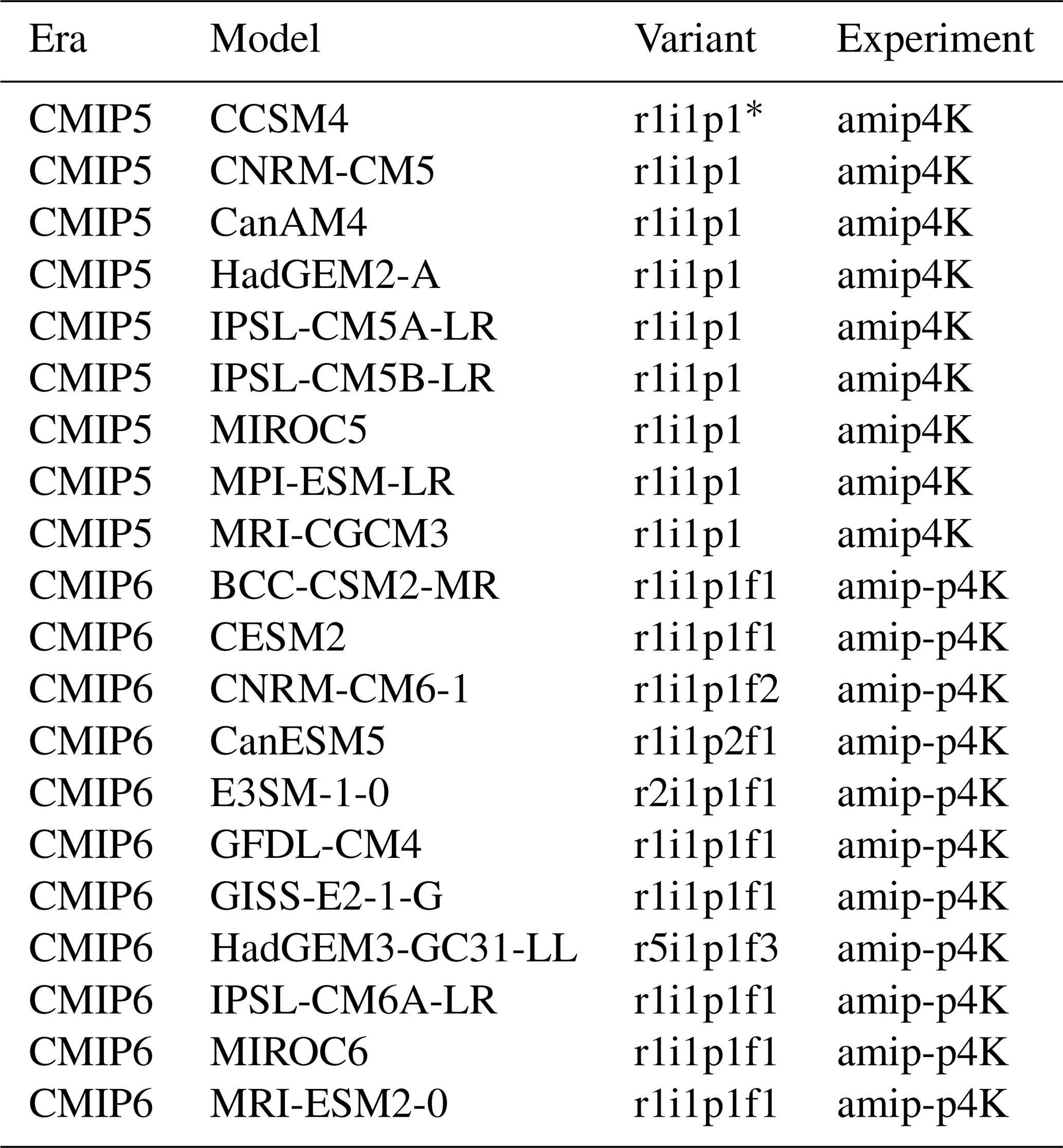
To compute cloud feedbacks, we make use of a pair of atmosphere-only experiments, one with prescribed observed sea surface temperatures (SSTs), sea ice concentrations, and radiative constituents (amip) and one that is identical but with the SSTs uniformly warmed by 4 K at each location (amip-p4K in CMIP6, amip4K in CMIP5). These experiments are part of the Cloud Feedback Model Intercomparison Project (CFMIP) protocol (Webb et al., 2017), but their roots can be traced back to early experiments to systematically diagnose feedbacks and climate sensitivity across an ensemble of atmospheric models (Cess et al., 1989, 1990). We compute the climatological monthly resolved cloud fraction histogram climatologies from both the control and perturbed experiments. These are then differenced, multiplied by cloud radiative kernels, and normalized by the change in annual-mean global-mean surface air temperature between the two experiments to compute cloud feedbacks. A total of 20 distinct models have provided sufficient data to compute cloud feedbacks in response to +4 K SST perturbations across CMIP5 and CMIP6 (Table 1). Cloud feedbacks computed using these atmosphere-only uniform SST perturbation experiments have been shown to give a close approximation to those simulated by fully coupled models in response to quadrupled CO2 (Ringer et al., 2014; Qin et al., 2022).
Table 1Models used in the calculation of cloud feedbacks. The asterisk indicates that for this model, the amip clisccp data are provided for the r7i1p1 member, but the amip4K clisccp data are provided for the r1i1p1 member. For all other models, the variant labels match between the control and +4 K amip experiment.
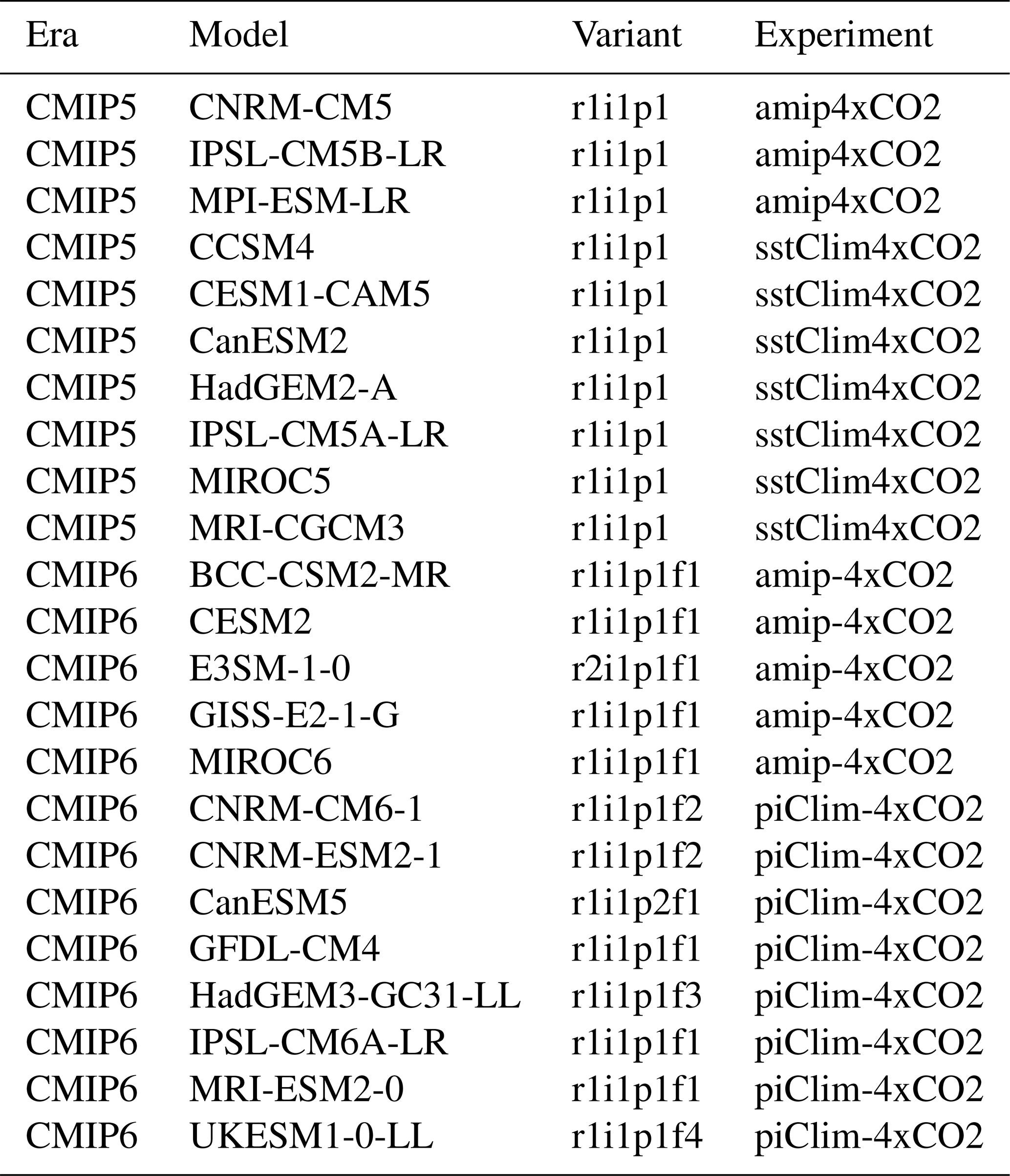
To compute rapid cloud adjustments, we make use of fixed SST atmosphere-only experiments with atmospheric CO2 levels quadrupled, for which there are two closely related experiment protocols in CMIP. The first protocol follows the CFMIP amip experiment and uses SST, sea ice, and radiative constituents set to their observed present-day values, except for CO2, which is quadrupled (referred to as amip-4xCO2 in CMIP6 and amip4xCO2 in CMIP5). These experiments are differenced with the amip experiment to compute “amip-type” rapid cloud adjustments. The second follows the Radiative Forcing Model Intercomparison Project (RFMIP) protocol (Pincus et al., 2016) and uses a repeating monthly resolved climatology of SST and sea ice concentration taken from each model's pre-industrial control (piControl) experiment as the prescribed boundary condition for each model. The baseline experiment and its quadrupled CO2 counterpart are known as piClim-control and piClim-4xCO2, respectively, in CMIP6 and sstClim and sstClim4xCO2, respectively, in CMIP5. As with the cloud feedback, we compute the climatological monthly resolved cloud fraction histogram climatologies from both the control and perturbed experiments. These are then differenced and multiplied by cloud radiative kernels to compute “piClim-type” rapid cloud adjustments. Note that unlike for cloud feedbacks, these anomalies are not normalized by the change in annual-mean global-mean surface air temperature since they are considered a part of the effective radiative forcing. We take all available models that did either of these experiments and provided the necessary output. For the 10 models that provided sufficient output for both the amip-type and piClim-type experiments, we use only results from the latter, yielding 23 distinct models (Table 2). Aside from the exceptions noted below, our results are unchanged when instead using the amip-type experiments from these 10 models, suggesting that rapid cloud adjustments do not significantly depend on this experimental design choice.
Table 2Models used in the calculation of rapid cloud adjustments.
2.2 Accounting for obscuration
Here we briefly review the approach for accounting for obscuration effects, closely following Scott et al. (2020). Given that a portion of the low-cloud field may be obscured by upper-level clouds, let us define an unobscured low-cloud fraction (LU) as
where L is the retrieved low-cloud fraction, and F is the total upper-level clear-sky fraction, defined as 1 minus the cloud fraction summed over all upper-level p and all τ. The precise definition of upper- and lower-level clouds is not prescribed and can vary depending on the context or needs (e.g., Myers et al., 2021; Ceppi et al., 2024). In practice, we use a cut-off of 680 hPa to delineate the two cloud types and refer to the resulting feedbacks or adjustments as being due to “low” or “non-low” clouds. When speaking more generally, we will use the more descriptive “lower-level” and “upper-level” descriptors. LU is the fraction of low clouds within the unobscured portion of a grid box and requires no assumptions about how clouds overlap. Note that at a given location and time , whereas F is a scalar. These cloud fractions are defined only in the case of grid-scale histograms, which are constructed by aggregating over many individual scenes (satellite pixels or model sub-columns) that are classified as either completely clear or completely covered by a cloud at a single level.
The low-cloud fraction can be expressed as the sum of a temporal mean (indicated with an overbar) and a temporal perturbation (denoted by a prime),
which means that anomalies in low-cloud cover can be expressed as
Next, we further decompose each term on the right-hand side (RHS) of Eq. (3) into a mean state and a perturbation, so that
The first term on the RHS of Eq. (6) is the change in the retrieved low-cloud fraction due solely to a change in unobscured low-cloud fraction. We consider the radiative responses resulting from this component to be closer to a “true” low-cloud response occurring in regions that are not obscured by upper-level clouds, which receive no contribution from changes in non-low-cloud coverage. Recall that this term represents the low-cloud fraction as a joint function of cloud top pressure and optical depth. Therefore, we can further break this down into amount, altitude, optical depth, and residual components following Zelinka et al. (2012b, 2013). As will be shown below, the modification to account for obscuration mostly affects the low-cloud amount component, with tiny impacts on the low-cloud altitude and optical depth responses.
The second term on the RHS of Eq. (6) is the change in the retrieved low-cloud fraction due solely to a change in total upper-level cloud fraction (i.e., obscuration). TOA radiative changes due to this obscuration-induced component of low-cloud response arise entirely from changes in upper-level cloud fraction that reveal or hide lower-level clouds. Hence by definition it is solely an amount component due to changes in non-low-cloud coverage. We therefore absorb this component into the non-low-cloud amount response, as we have previously done in Zelinka et al. (2022). As will be shown below, the modified non-low-cloud amount feedback is typically less negative/more positive than the original non-low-cloud amount component, and vice versa for the rapid adjustment. One can think of this as the non-low-cloud amount component reclaiming a portion of the low-cloud radiative response that arises solely due to changes in obscuration.
The third term in parentheses on the RHS of Eq. (6) is a term due to covarying changes in the lower- and upper-level cloud fields and is typically very small.
Written more plainly, the original low-cloud response decomposed in Eq. (6) can be expressed as
where lowamt, lowalt, lowtau, and lowerr refer to the amount, altitude, optical depth, and residual components of the low-cloud response, respectively, which are computed following the approach detailed in Appendix B of Zelinka et al. (2013). The subscript “unobsc” refers to the fact that these components are all occurring in scenes that are not obscured by upper-level clouds, calculated using the first term on the RHS of Eq. (6) (). Δobsc represents the change in obscuration, diagnosed from the second term on the RHS of Eq. (6) (), and cov is the covariance term, diagnosed from the third term on the RHS of Eq. (6) (). In an effort to preserve the total number of components from the original decomposition, and given that the covariance term is typically very small, we combine the covariance and residual terms into a single modified residual term (low) such that the modified low-cloud response can be expressed as
Similarly, incorporating Δobsc into the original non-low-cloud amount response yields the modified non-low-cloud response:
where non-low is the sum of the original non-low-cloud amount response and the change in obscuration term.
To summarize, the total cloud response can be expressed as
and the original and modified cloud responses are related as follows:
In Appendix A, we derive analogous expressions for the case of three vertical cloud layers (low, middle, and high). Below we will compare the original and modified low and non-low-cloud responses, which primarily illustrates the impact of moving the obscuration term from the low-cloud response to the non-low-cloud response.
We first provide a physical interpretation of the impacts of changes in obscuration on the low- and high-cloud responses diagnosed with cloud radiative kernels applied to cloud property histograms derived from passive satellites (or produced by passive satellite simulators in models). For simplicity, let us consider only SW radiation in these examples. First, consider a scene with an opaque high cloud completely overlapping an opaque low cloud (Fig. 1a). Assume that the high-cloud fraction decreases with warming, but the low-cloud fraction remains unchanged. The high-cloud decrease will reveal some portion of low cloud that was previously not exposed to space (Fig. 1b). This apparent increase in lower-level cloud will constitute a negative radiative response despite the fact that the actual low-cloud amount remained unchanged. Hence, the low-cloud amount response diagnosed from the cloud radiative kernel (CRK) technique using the original decomposition will be biased negative relative to the actual, unobscured value, which is close to zero1 (Fig. 1d). Note that this scenario would be indistinguishable from the (extremely rare) scenario in which control-state low-cloud cover is truly zero but then increases to a nonzero value in the perturbed climate.
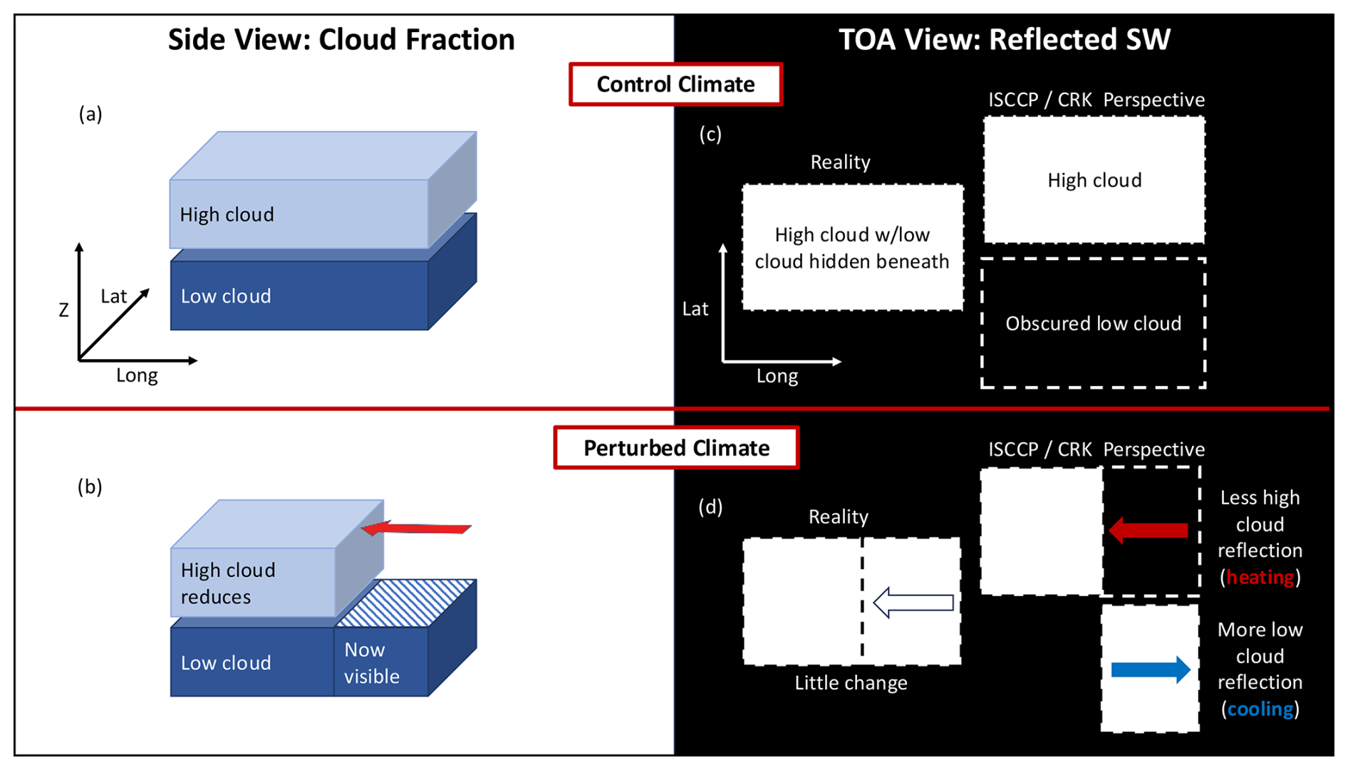
Figure 1Schematic demonstrating the effects of changing obscuration on cloud feedbacks and adjustments diagnosed by cloud radiative kernels. In this scenario, a high cloud completely overlaps a low cloud in the mean climate but decreases with climate warming so as to reveal a portion of the (unchanged) low cloud.
Because cloud radiative kernels are constructed by differencing TOA radiative fluxes calculated assuming completely overcast and clear-sky scenes in a radiative transfer model, they quantify the change in TOA radiation due to changes in cloud cover with the implicit assumption that these changes are relative to a clear-sky atmosphere. The CRK technique will therefore produce a positive radiative impact from high-cloud reductions occurring over the typically darker Earth surface (recall that we are only considering SW effects in this discussion). Hence, in this hypothetical scenario, the radiative response from decreases in high-cloud cover as diagnosed using the original approach will be biased positive relative to the true value (Fig. 1d). This is because the removal of a high cloud above a bright low cloud leads to a much smaller decrease in SW reflection than if it is above clear sky. The obscuration adjustment, therefore, is essentially correcting for the kernel overestimate of the high-cloud amount response by adding back in the radiative impact of the clouds that are revealed below. This will restore this response to something closer to zero, as will be seen below.
Similarly, consider another scenario with an opaque high cloud partially overlapping an opaque low cloud (Fig. 2a). Assume the high cloud increases but the low-cloud fraction remains unchanged (Fig. 2b). The high-cloud increase will hide low cloud, and this apparent decrease in lower-level cloud fraction will constitute a positive radiative response despite the fact that the actual low-cloud amount remained unchanged (Fig. 2d). Hence the low-cloud amount response will be biased positive relative to the true unobscured low-cloud amount response. Moreover, due to the aforementioned implicit assumption of hiding/revealing clear skies in the CRK approach, the radiative response from increases in high-cloud cover will be biased negative (by roughly the same amount).
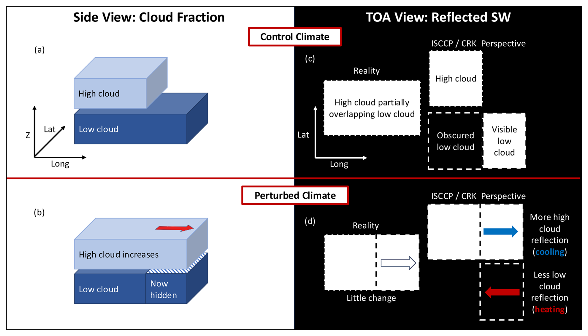
Figure 2As in Fig. 1 but for a scenario in which a high cloud partially overlaps a low cloud in the mean climate but increases in the perturbed climate so as to completely obscure the (unchanged) low cloud.
In all of these examples, actual low-cloud changes were zero simply for the sake of isolating the role of changes in obscuration alone in low- and high-cloud responses. More typically, there are real low-cloud responses operating alongside obscuration effects. Moreover, we only discussed SW effects owing to their simplicity and because they are more relevant. This is because low clouds have a small longwave (LW) effect, so changes in the obscuration of low clouds by upper-level clouds have a much smaller effect on the LW fluxes reaching the TOA. The LW flux emanating from a low-cloud scene is not much different from that emitted from a clear-sky scene. Hence if a high cloud covers up a low cloud, the radiative impact is well captured by the LW CRK. The same cannot be said for the SW.
There are other issues that arise from the use of passive satellite datasets and their respective simulators that cannot be corrected for with the output we have. Most notably, the ISCCP simulator only reports a single cloud layer for each scene, regardless of whether the scene has multi-layer clouds. This single cloud is assigned a cloud top pressure with a temperature corresponding to the scene's infrared brightness temperature. This introduces two well-known issues: first, clouds under a strong inversion are often placed too high in the atmosphere, at the higher level at which this temperature is found (Garay et al., 2008). Second, in multi-layer cloud scenes in which a non-opaque high cloud overlies lower-level clouds, the simulator often places a single cloud at middle levels since the brightness temperature will reflect some combination of warm lower-level cloud and the cold but thin upper-level cloud (Pincus et al., 2012; Marchand and Ackerman, 2010). Finally, as noted above, the ISCCP retrieval algorithm reports a single cloud layer with a cloud optical depth equal to the column-integrated optical depth, even if multiple cloud layers are present in a given scene. This implies that some portion of the change in upper-level cloud properties as reported by the simulator (and subsequently diagnosed as non-low-cloud feedbacks or adjustments) may in fact be partly induced by changes in lower-level cloud properties. Hence, even with the aforementioned corrections, one should not consider the modified feedbacks derived herein as strictly “true” non-low- and low-cloud feedbacks, owing to the additional issues that we cannot correct for.
4.1 Cloud feedbacks
Having motivated our modified cloud feedback calculations and given schematic illustrations of the diagnostic issues they are intended to mitigate, we now turn to examining the impacts of these modifications on the cloud feedbacks diagnosed in climate models. In Fig. 3 we show the multi-model-mean original and modified net (longwave plus shortwave) non-low- and low-cloud amount feedbacks. The difference between modified and original is also shown, which provides a measure of how large the obscuration effect is.
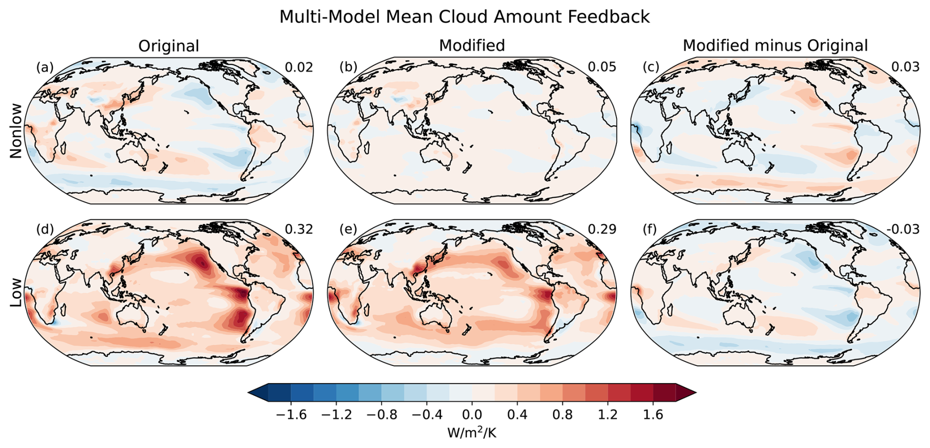
Figure 3Multi-model-mean non-low-cloud amount feedback computed using the original methodology (a) and using the modified methodology (b), along with their difference (c), which measures the effect of obscuration changes on the feedback. The corresponding feedbacks for low clouds are shown in panels (d)–(f). Global-mean values are displayed at the top right of each map.
The modified low-cloud amount feedback is somewhat muted relative to the original low-cloud amount feedback (Fig. 3d and e). The large positive low-cloud amount feedbacks over the NE and SE Pacific stratocumulus decks and over the Southern Ocean are weaker once accounting for obscuration effects. The interpretation is that, on average, the warming-induced increase in high-cloud coverage over regions of persistent low-cloud cover (most prominently, NE Pacific, SE Pacific, west of Namibia, and over the Southern Ocean) hides a portion of the underlying low clouds. In the original decomposition, this contributes to a positive low-cloud amount feedback, augmenting the positive unobscured low-cloud amount feedback from actual decreases in low-cloud cover. However, in some regions like east of Australia, the positive modified low-cloud amount feedback is larger than its original version (Fig. 3d and e). In these regions, decreases in non-low clouds reveal low clouds beneath. In the original decomposition, this contributes negatively to the low-cloud amount feedback, diminishing the positive unobscured low-cloud amount feedback from actual decreases in low-cloud cover.
By definition (see Eqs. 11 and 12), the corrections applied to the low-cloud feedback are equal and opposite to those applied to the non-low-cloud feedback. The same is true to a very close approximation for the amount components such that what is taken away from the low-cloud amount feedback is given to the high-cloud amount feedback (i.e., Fig. 3c and f are equal but opposite in sign). Therefore, the high-cloud amount feedback is restored to something very close to zero are nearly every location (Fig. 3b), as expected from changes in coverage of clouds with closely canceling longwave and shortwave effects. The distinct regions of negative high-cloud amount feedback over the stratocumulus regions of the NE and SE Pacific and over the Southern Ocean, along with the regions of positive high-cloud amount feedback over east Asia, South America, Africa, and east of Australia are all essentially absent from the modified version (Fig. 3a and b). That the global-mean value is closer to zero in the original calculation is due to a fortuitous cancellation between larger positive and negative regional values.
At nearly all locations, but especially over the ocean, the inter-model spread in both the non-low- and low-cloud amount feedbacks is reduced in the modified calculation (Fig. 4). This is because the original low-cloud amount feedback in these regions is positively correlated with the change in obscuration (see Eq. 11), reflecting the fact that models with larger increases in obscuration experience a larger augmentation of the unobscured positive low-cloud feedback, and vice versa. By removing these obscuration effects, the modified low-cloud feedback is uncorrelated with the change in obscuration and therefore exhibits less inter-model spread (Fig. A1b). Conversely, the original non-low-cloud amount feedback in these regions is negatively correlated with the change in obscuration (see Eq. 12), reflecting the fact that models with larger increases in obscuration experience a larger negative bias with respect to the modified non-low-cloud amount feedback, and vice versa. By removing these obscuration effects, the strong anti-correlation between non-low-cloud feedback and the change in obscuration vanishes, and therefore the modified non-low-cloud feedback exhibits less inter-model spread (Fig. A1a).

Figure 4Across-model standard deviation of non-low-cloud amount feedback computed using the original methodology (a) and using the modified methodology (b), along with their difference (c). The corresponding feedbacks for low clouds are shown in panels (d)–(f). The rectangular box indicates the averaging region for the data presented in Fig. A1, chosen because it is a prominent region of reduced spread in the modified decomposition.
Given the reduction in inter-model spread in the modified low-cloud amount feedback at most locations (Fig. 4f), do the cloud types and/or regions that most contribute to the inter-model spread of global-mean cloud feedback change? To answer this, we compute the across-model variance explained between the global-mean total net cloud feedback and grid-point values of the non-low and low net cloud amount feedbacks, for both the original and modified methodologies, closely following Soden and Vecchi (2011). As expected from previous studies, the spread in global-mean net cloud feedback is strongly related to the low-cloud amount feedback in regions of prevalent low cloud, including the subtropical and midlatitude oceans (Fig. 5d). The modified methodology highlights the same regions, but the variance explained is larger nearly everywhere, especially over the Atlantic and Indian oceans, subtropical South Pacific, equatorial Pacific cold tongue, and North Pacific (Fig. 5e and f). The modification also results in a reduction in the variance explained by non-low clouds over the subtropical Atlantic Ocean (Fig. 5c). This may provide further evidence of the importance of properly accounting for obscuration effects, as it leads to a clearer attribution of inter-model spread to its true source (low clouds).
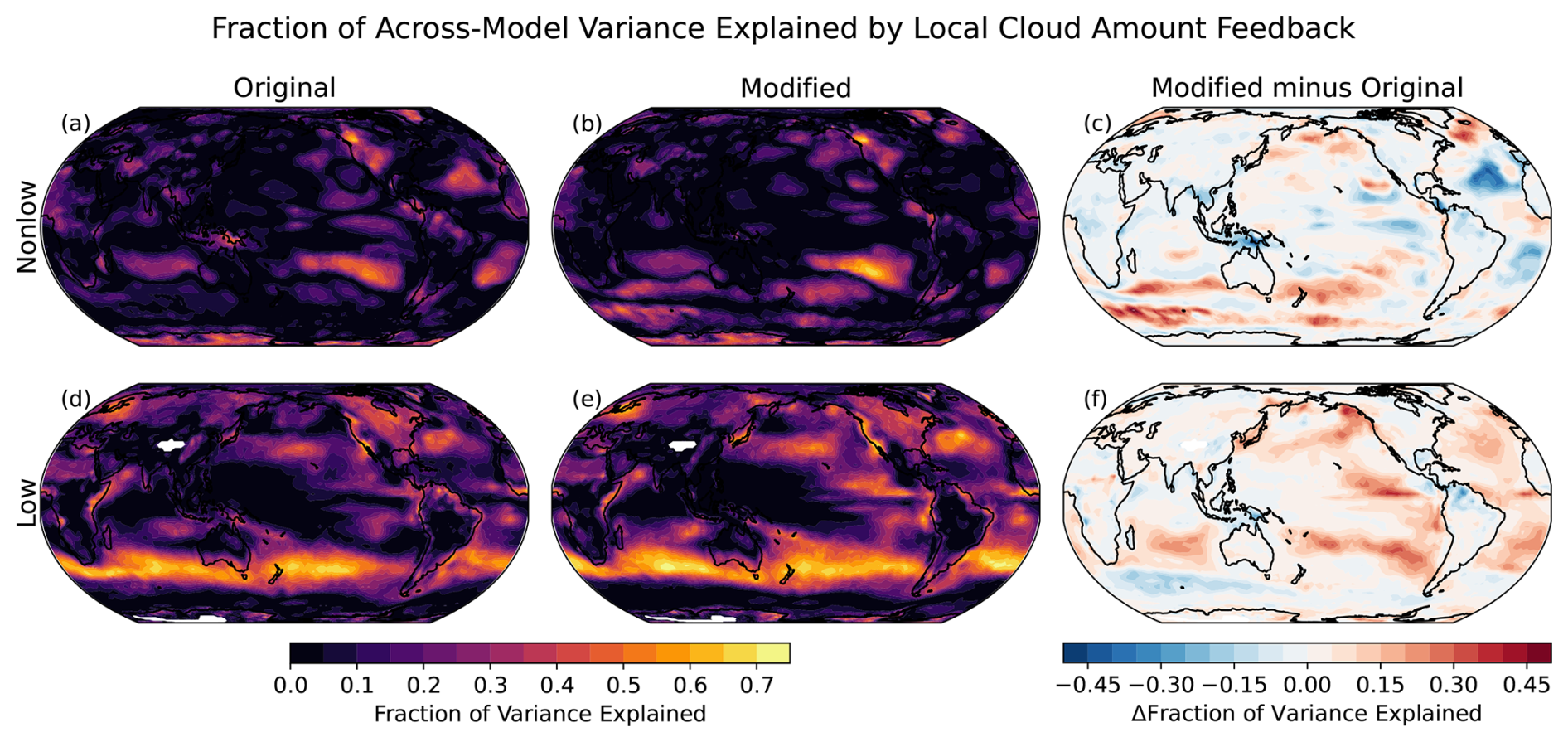
Figure 5Fraction of across-model variance in global-mean net cloud feedback explained by local net (a–c) non-low-cloud amount feedback and (d–f) low-cloud amount feedback using the (a, d) original and (b, e) modified methodology. In the right column (c, f), we show the difference between modified and original methodologies.
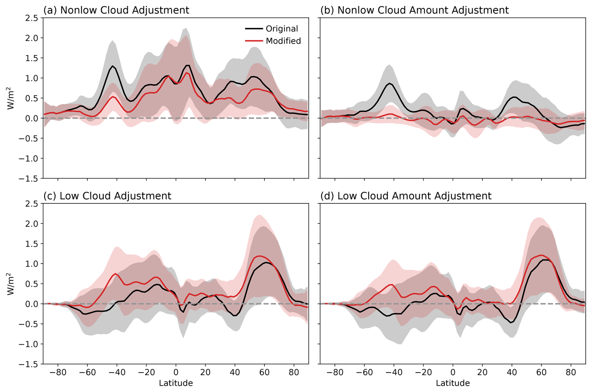
The low-cloud amount feedback is much less positive poleward of about 50° in either hemisphere after accounting for obscuration effects (Fig. 6d). This makes the positive low-cloud feedback much more confined to low latitudes and the negative lobe at middle to high latitudes much more robust (Fig. 6c). Similarly, the latitudinal dipole in non-low-cloud amount feedback centered near 50° in either hemisphere is completely removed (Fig. 6b). Physically, this may be related to the poleward shift of high clouds in the midlatitude storm track. Without accounting for change in obscuration of underlying clouds, the radiative kernel diagnoses radiative heating on the equatorward flank of the jet (where high clouds vacate) and a radiative cooling on the poleward flank (where high clouds increase). The modified non-low-cloud feedback is much more muted because it accounts for the fact that these high-cloud anomalies are occurring in a region of prevalent low-cloud cover (Tselioudis et al., 2016). Specifically, the regions vacated by high clouds reveal bright low clouds rather than dark ocean surface, limiting the size of the positive radiative anomaly attributable to high clouds near 40°. The regions experiencing increased high-cloud cover on the poleward flank have hidden bright low clouds rather than a dark ocean surface, limiting the size of the negative radiative anomaly attributable to high clouds near 60°.
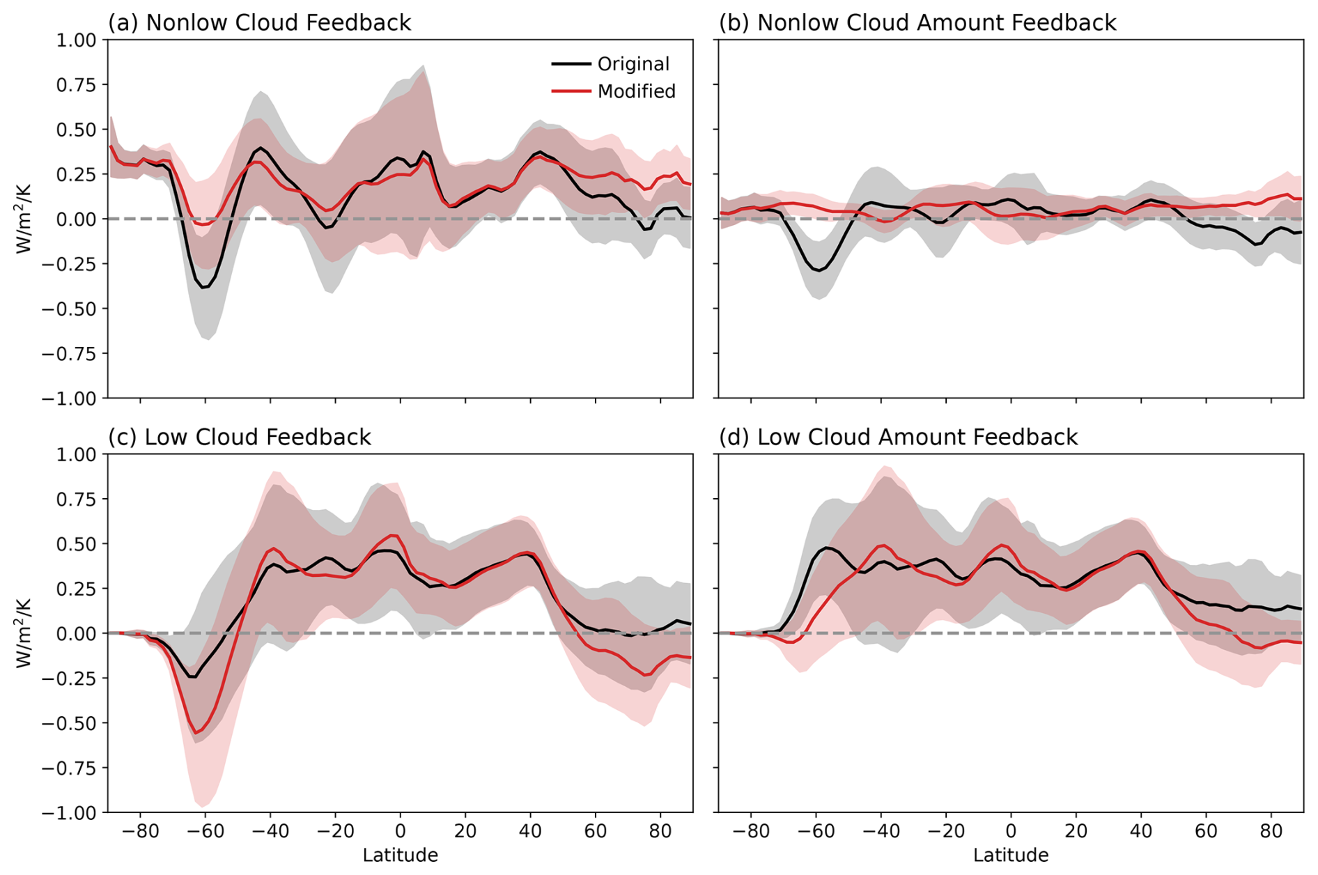
Figure 6Zonal mean non-low- and low-cloud feedbacks and their amount components, computed using the original (black) and modified (red) decompositions. Solid lines represent the multi-model means, and the shading spans the ±1σ range across models.
In Fig. A2 we demonstrate the impact of our modified calculations on the distribution of global-mean cloud feedback components across models. Accounting for obscuration primary affects the low and non-low SW and net cloud feedbacks via the amount component, with all other feedback components being either identical to the original calculation (by design) or indistinguishable from them. On average, the low-cloud amount component becomes slightly smaller, while the non-low-cloud amount feedback becomes slightly larger. Both components exhibit less inter-model spread in the modified calculations.
While the global-mean and multi-model-mean feedbacks are not strongly affected by the modified calculations, this belies substantial changes apparent at local scales (Figs. 3 and 6) and within individual models (Fig. 7). For most models, the original calculation overestimates the positive low-cloud amount feedback, as evidenced by the models for which the black bars extend beyond the red markers in Fig. 7d. This occurs as a result of increased obscuration by non-low clouds. However, this is not true for all models, as some show little effect of changing obscuration (at least in the global mean), and several show the opposite effect: most notably, HadGEM3-GC31-LL experiences decreased obscuration by non-low clouds, so the modified low-cloud amount feedback is actually considerably larger than the original calculation. This model now has the largest low-cloud feedback of all models rather than a near-average value (Fig. 7c). In the case of low-cloud feedback and its amount component, accounting for obscuration affects the magnitude but not the sign of the feedback in all models.
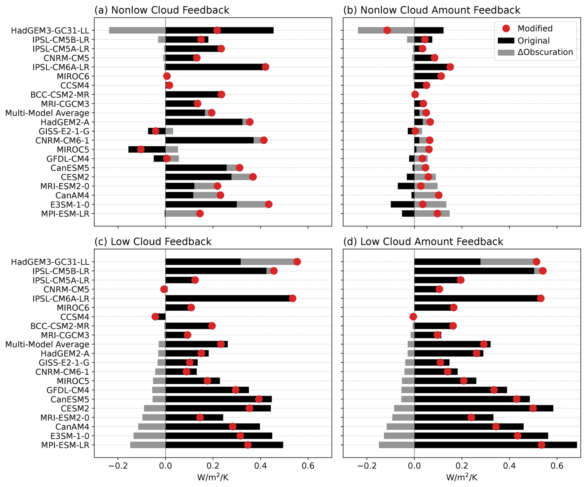
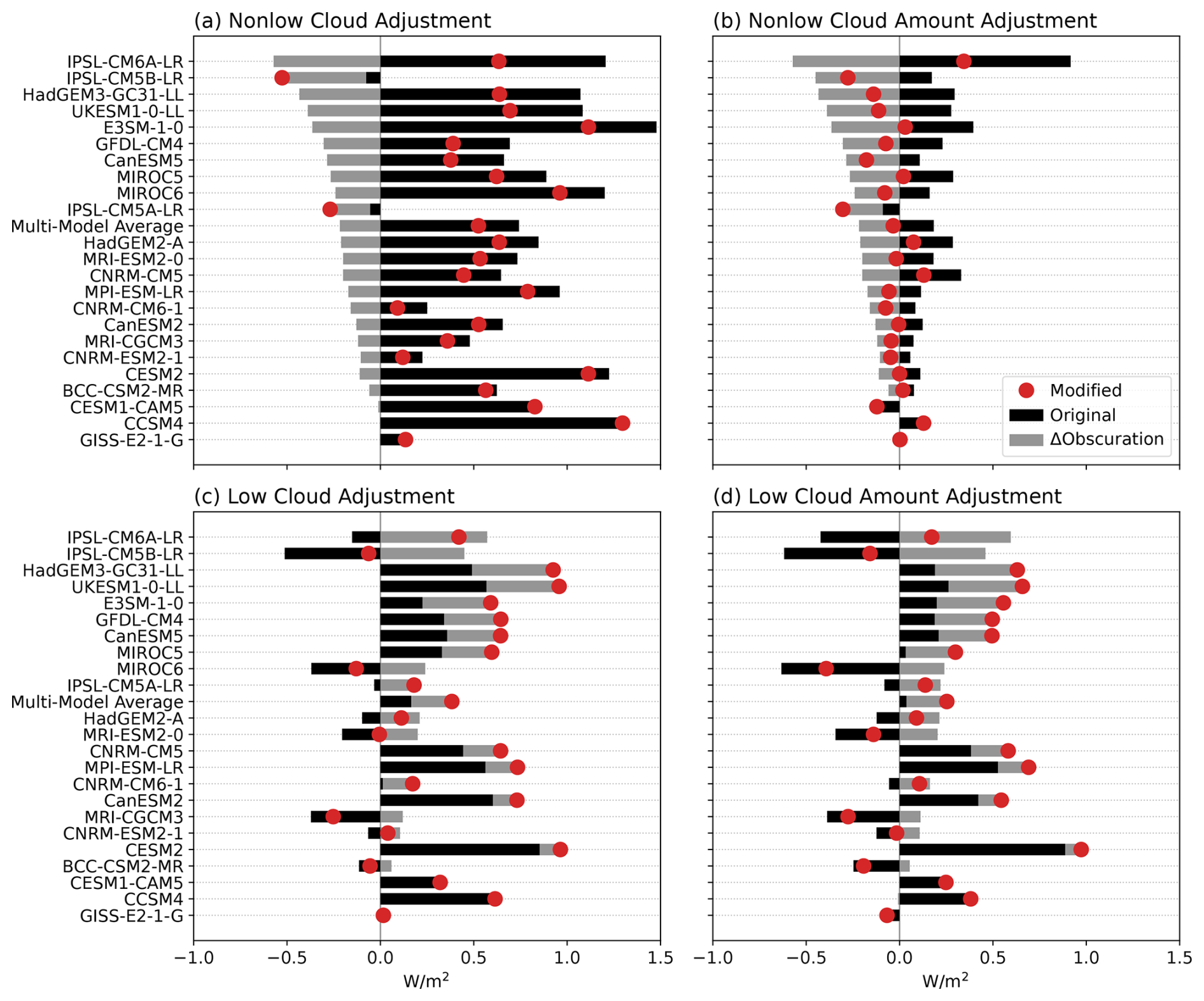
Figure 7Global-mean non-low- and low-cloud feedbacks and their amount components computed using the original (black) and modified (red) decompositions, along with their difference (gray). Models are ordered by the strength of their obscuration adjustment. Note that the sign of the ΔObscuration term is defined in both rows as the modified minus original feedback, which is opposite to the definition in Eq. (11).
This is not generally the case for the non-low-cloud amount feedback (Fig. 7b). Several models with negative non-low-cloud amount feedbacks in the original decomposition actually have positive feedbacks in the modified calculation. There is much stronger across-model agreement that the non-low-cloud amount feedback is positive in the modified calculation. While the non-low-cloud amount feedback is small regardless of which decomposition is used, accounting for obscuration can substantially change the overall non-low-cloud feedback in some models (Fig. 7a). For example, MPI-ESM-LR's non-low-cloud feedback increases from near-zero to a moderate positive value, while HadGEM3-GC31-LL's large positive non-low-cloud feedback is roughly halved.
Total inter-model variance of global-mean cloud feedback remains unchanged regardless of the decomposition, so decreasing variance in both non-low- and low-cloud amount feedbacks (with negligible change in altitude, optical depth, and residual components) implies that something else must compensate. In the original decomposition, low-cloud amount feedback is strongly anti-correlated with the low-cloud optical depth component and especially with the non-low-cloud amount component (Fig. 8). The latter reflects the fact that increased upper-level cloud cover was hiding lower-level clouds beneath, making the low-cloud feedback appear larger. Properly accounting for obscuration effects removes this anti-correlation (Fig. 8). So, while the variance in non-low- and low-cloud amount feedback have decreased in the modified decomposition, so too has the large negative covariance among several feedback components. This might suggest that the modified decomposition better reveals sources of spread and reduces apparent covariances that may be more artificial than physical, analogous to the fixed relative humidity radiative feedback framework of Held and Shell (2012).
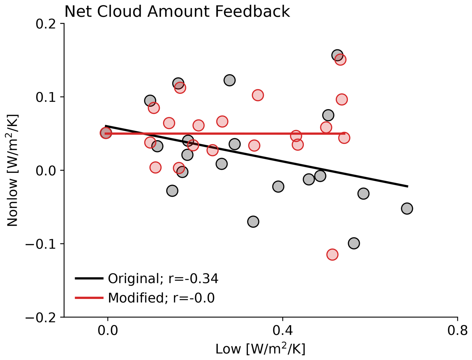
Figure 8Global-mean net cloud amount feedbacks for non-low clouds scattered against those for low clouds.
4.2 Rapid cloud adjustments
As noted earlier, cloud adjustments that occur rapidly after the step change in CO2 concentration impart radiative effects that are typically included as part of the effective radiative forcing. In Fig. 9, we show the multi-model-mean low and non-low-cloud adjustments as computed using the original and modified decomposition, along with their difference. The low-cloud rapid adjustment is strongly negative over ocean due to increases in lower-level cloud cover and positive over land due to large reductions in low-cloud cover (Fig. 9d). As noted in Zelinka et al. (2013), a portion of the large increase in lower-level cloud cover over the ocean that is diagnosed by the ISCCP simulator is actually a result of decreased obscuration. This is because non-low clouds, especially those in the mid-troposphere, decrease in response to the radiative warming and attendant drying from CO2 (Colman and McAvaney, 2011; Wyant et al., 2012; Kamae and Watanabe, 2012; Kamae et al., 2015). This effect of changing obscuration is confirmed in Fig. 9, where the large negative oceanic low-cloud amount adjustment is substantially reduced when accounting for obscuration changes (compare Fig. 9d and e). The global- and multi-model-mean rapid low-cloud adjustment is increased from near zero to 0.25 W m−2, due to a widespread reduction in the negative oceanic values with little change in the large positive values over land (which do not result from obscuration changes).
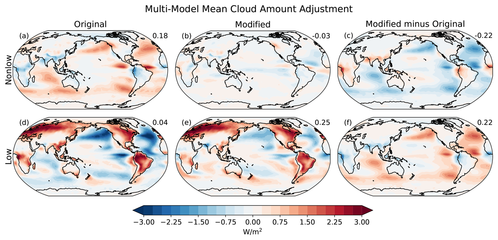
Figure 9As in Fig. 3 but for rapid cloud adjustments.
Complementing this result, the modified non-low-cloud adjustment is much closer to zero than in the original decomposition. Rapid decreases in non-low-cloud amount reveal low clouds, making the net radiative adjustment small (Fig. 9b). This contrasts with the original calculation which essentially assumes that the rapid reduction in non-low clouds reveals a dark ocean beneath, causing a large positive radiative adjustment (Fig. 9a). Hence, averaged globally and across models, the partitioning of the positive rapid cloud adjustment completely switches from being dominated by non-low clouds and a small contribution from low clouds (Fig. 9a and d) to being dominated by a large positive low-cloud contribution that is opposed slightly by a small non-low-cloud contribution (Fig. 9b and e).
As was the case for the cloud feedback, the low and non-low rapid cloud adjustments exhibit less inter-model spread at nearly every location on the globe (Fig. 10). This can be understood through the arguments discussed above for the cloud feedback, which will not be reiterated here.
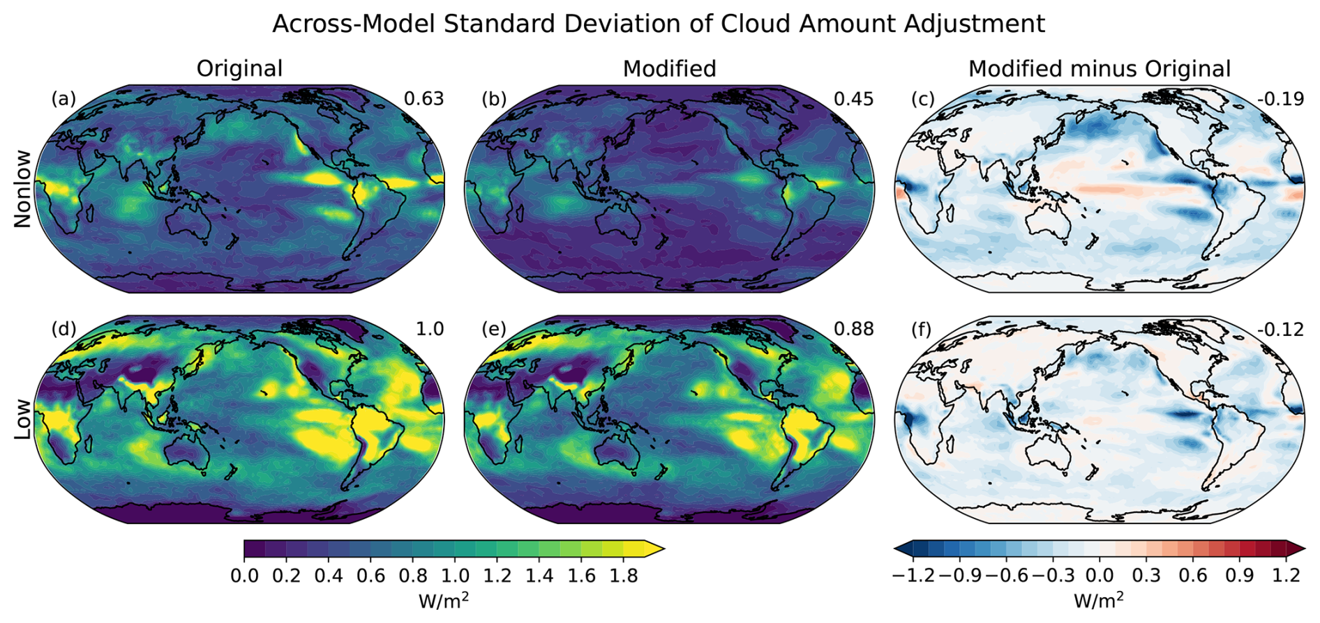
Figure 10As in Fig. 4 but for rapid cloud adjustments.
Examining the zonal mean rapid cloud adjustments, we see that the modified low-cloud adjustment and its amount component, which dominates the response, are systematically shifted toward positive values at all latitudes but most especially in the Southern Hemisphere middle latitudes (Fig. 11c and d). Similarly, the modified non-low-cloud amount adjustment is shifted to be very close to zero at every latitude, and the large values in either hemisphere around 40° latitude apparent in the original decomposition are now completely removed (Fig. 11b).
Distributions of global-mean rapid cloud adjustments for non-low and low clouds are shown in Fig. A3. Similar to the cloud feedbacks, the modified calculations cause the largest changes for the net and SW amount components. In particular, the distribution of SW and net low-cloud amount adjustments shifts from being centered on zero to a positive value, as this calculation no longer allows decreased non-low-cloud coverage from aliasing itself onto the low-cloud rapid adjustment. Similarly, the SW and net non-low-cloud amount adjustment distribution shifts downward from a moderate positive value to something closer to zero. This weaker positive non-low-cloud adjustment is because rapid reductions in non-low clouds reveal lower-level clouds in the modified decomposition, whereas they are assumed to reveal a dark ocean in the original decomposition.
As noted above for the cloud feedback, the impact of accounting for obscuration effects varies substantially among models. Unlike for the cloud feedback, however, the effect is uniform in sign across models. Specifically, in all models, rapid decreases in non-low-cloud fraction reveal more low clouds, making the original low-cloud adjustment weaker positive or stronger negative, as indicated by the red circles being located to the right of the black bars in Fig. 12c. This is evidence of the effect illustrated schematically in Fig. 1. In many models, the original small positive low-cloud amount adjustment more than doubles in the modified calculation, and several models' adjustments change sign from negative to positive. Similarly, the original non-low-cloud amount adjustment is positively biased (see Fig. 1) such that the modified adjustment is much smaller and in many models switches to a negative value (red circles to the left of black bars in Fig. 12b). While this sign change does not occur in any model for the overall non-low-cloud adjustment, the reduction in positive non-low-cloud adjustment strength remains apparent in Fig. 12a.
Rapid cloud adjustment terms are largely consistent between piClim- and amip-style quadrupled CO2 experiments, as shown for the models that conducted both in Fig. A4. However, for several models, the piClim-style experiments lead to larger positive low-cloud adjustments than the amip-style experiments. In these models, the rapid response of low and non-low clouds (but not of the obscuration) appears to depend on experiment design. We leave further exploration of why this is the case to future work.
In this study we presented a methodology for decomposing cloud feedbacks and rapid adjustments among low and non-low clouds that properly accounts for obscuration effects. This methodology has been used in previous studies (e.g., Zelinka et al., 2018, 2022; Scott et al., 2020; Myers et al., 2021; Chao et al., 2024), but the effect of these choices has not been formally documented across models to date. While the overall cloud feedbacks and adjustments do not depend on the methodology employed, and the decision to split the feedback among low and non-low clouds rather than some other decomposition is partly arbitrary, the impacts of these methodological choices are important because they can improve the mechanistic interpretation of the results and avoid artificial relationships that are not physical. In this sense the recommended methodology is analogous to the constant relative humidity feedback decomposition proposed by Held and Shell (2012), which reduces spread in water vapor, lapse rate, and Planck feedbacks and eliminates the anticorrelation between lapse rate and water vapor feedbacks, revealing more clearly the dominant uncertainties in radiative feedbacks.
We find that the positive multi-model-mean low-cloud feedback is weaker in our modified calculations because it excludes the positive radiative contribution from apparent reductions in low clouds that are due solely to increased obscuration by non-low clouds. Complementing this, the non-low-cloud feedback is much closer to zero at every location in our modified calculation, as changes in non-low clouds have a muted radiative impact when occurring over low clouds. Across models, the strength and in some cases even the sign of the low and non-low-cloud feedbacks change, and an apparent anti-correlation between low- and non-low-cloud amount feedbacks is removed when accounting for obscuration. Finally, the inter-model variance in both non-low- and low-cloud feedbacks is damped in nearly all locations when properly accounting for obscuration effects.
Upon quadrupling of CO2, large decreases in oceanic upper-level cloud coverage reveal underlying lower-level clouds. In the original decomposition this leads to an apparent negative oceanic low-cloud radiative adjustment that is solely due to reduced obscuration. Properly accounting for obscuration, however, strongly reduces this negative adjustment, leading to a moderate positive low-cloud adjustment in the multi-model mean. Moreover, the positive non-low-cloud radiative adjustment from the large reduction in non-low clouds in the original decomposition is substantially weakened in the modified calculations, such that the modified non-low rapid cloud adjustment is very close to zero at all locations. Hence, in the multi-model mean, the rapid cloud adjustment to quadrupled CO2 arises from a large positive low-cloud radiative adjustment countered only slightly by a weak negative non-low-cloud radiative adjustment. As was the case with cloud feedbacks, the inter-model variance in both non-low- and low-cloud adjustments is damped in nearly all locations when properly accounting for obscuration effects, most notably over the oceans.
Given that neglect of obscuration effects can lead to misleading results regarding the attribution of feedbacks and adjustments to specific cloud types or physical processes and, in most locations, inflates the inter-model variance in these, we recommend that the community follows the methodology presented herein when computing low- and non-low-cloud feedbacks and adjustments using cloud radiative kernels. It must be borne in mind, however, that no decomposition that relies on cloud information from passive satellite retrievals can ensure that the radiative effect attributed to a given cloud type is solely due to changes in that cloud type, owing to nonlinear aspects of radiation. Nevertheless, addressing obscuration effects is an important step in this direction. Code to perform this decomposition and a Jupyter notebook to demonstrate the calculations is available at the URL provided in the “Code availability” section.
One may choose to decompose feedbacks or adjustments into contributions from high (H), middle (M), and low (L) clouds. In this case we define the upper-level clear-sky fraction as
in which case Eq. (6) becomes
where ϵ contains the covariance terms. Unobscured mid-level clouds will have a form similar to Eq. (1),
where
We can then decompose M′ in a form similar to Eq. (6):
which is equivalent to
There are now a total of three obscuration terms in Eqs. (A2) and (A6): is a mid-level cloud response that reveals or obscures underlying low clouds, is a high-level cloud response that reveals or obscures underlying low clouds, and is a high-level cloud response that reveals or obscures underlying mid-level clouds. As before, if we include the obscuration of lower clouds by a middle or high cloud as part of the mid- or high-cloud feedback (and omitting covariances), we get
This ensures that the sum of the three modified cloud responses is equal to the total cloud response.
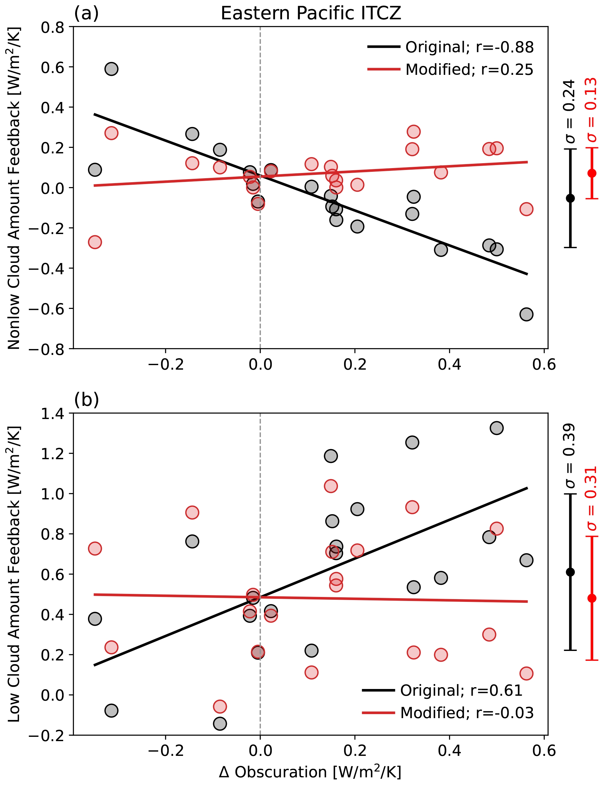
Figure A1Net cloud amount feedbacks for (a) non-low and (b) low clouds averaged over the Eastern Pacific Intertropical Convergence Zone (ITCZ) region indicated in Fig. 4 scattered against the coincident change in obscuration. Feedbacks computed using the original and modified decomposition are shown with black and red markers, respectively. Error bars to the right indicate the multi-model mean and standard deviation of original and modified feedbacks.
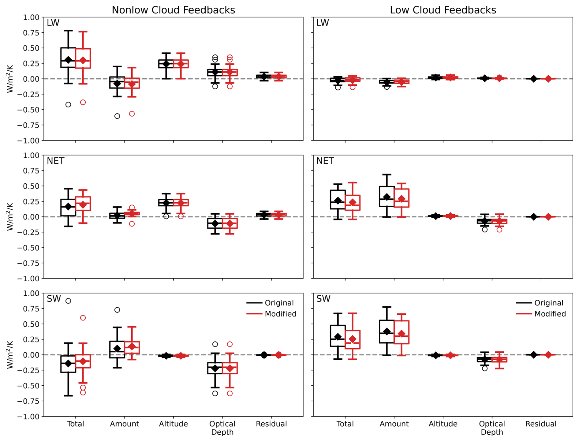
Figure A2Box-and-whisker plots summarizing the distribution of global-mean non-low- and low-cloud feedbacks across models. Feedbacks are separated into LW, SW, and net (LW + SW) components, each of which is further separated into components due to changes in amount, altitude, and optical depth, along with a residual term. Feedbacks are shown for the original calculation in black and the modified calculation in red. Each box extends from the first quartile to the third quartile of the data, with a line at the median and a diamond at the mean. The whiskers extend from the box to the farthest data point lying within 1.5 times the interquartile range from the box. Flier points are those past the end of the whiskers.
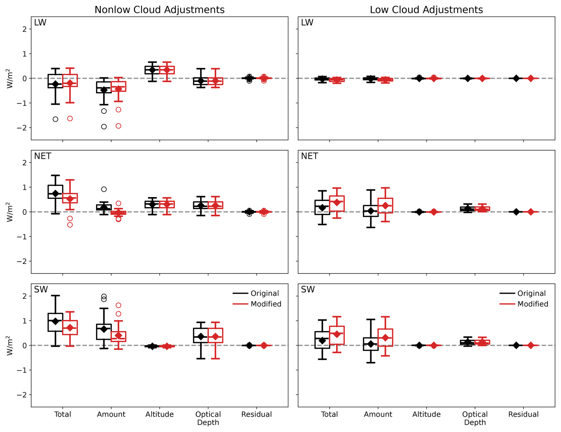
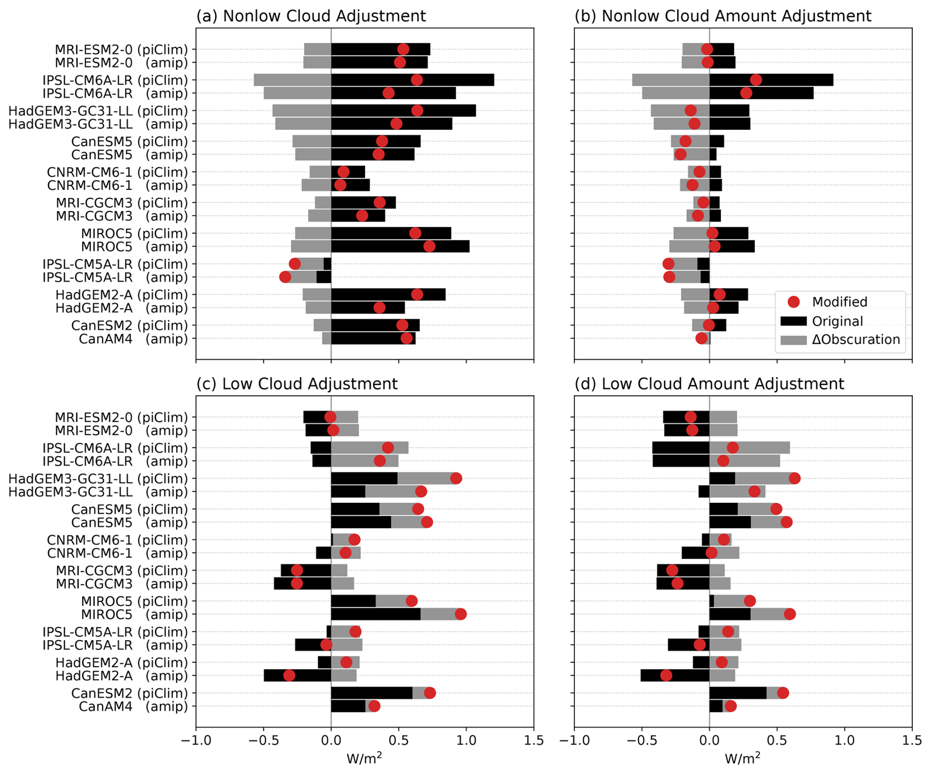
Figure A4As in Fig. 12 but comparing rapid cloud adjustments between piClim- and amip-style CO2 quadrupling experiments for models that performed both.
Cloud radiative kernels, along with the code to perform the calculations in this study, are available at https://doi.org/10.5281/zenodo.13686878 (Zelinka, 2024).
All CMIP climate model data used in this study are available at https://esgf.github.io/ (Earth System Grid Federation, 2024).
All analyses in the paper were performed by MDZ. The first draft of the manuscript was written by MDZ, and all the authors commented on subsequent versions of the manuscript. All the authors read and approved the final paper.
The contact author has declared that none of the authors has any competing interests.
The statements, findings, conclusions, and recommendations are those of the authors and do not necessarily reflect the views of NOAA or the US Department of Commerce.
Publisher's note: Copernicus Publications remains neutral with regard to jurisdictional claims made in the text, published maps, institutional affiliations, or any other geographical representation in this paper. While Copernicus Publications makes every effort to include appropriate place names, the final responsibility lies with the authors.
We thank two anonymous reviewers for their helpful comments that improved the manuscript. We acknowledge the World Climate Research Programme, which, through its Working Group on Coupled Modeling, coordinated and promoted CMIP. We thank the climate modeling groups for producing their model output and making it available, the Earth System Grid Federation (ESGF) for archiving the data and providing access, and the multiple funding agencies who support CMIP and ESGF. The work of Mark D. Zelinka and Li-Wei Chao was performed under the auspices of the US DOE by Lawrence Livermore National Laboratory under contract DEAC52-07NA27344. The Pacific Northwest National Laboratory is operated for the DOE by the Battelle Memorial Institute under contract DE-AC05-76RL01830.
Mark D. Zelinka, Li-Wei Chao, and Yi Qin were supported by the US Department of Energy (DOE) Regional and Global Model Analysis program area. Timothy A. Myers was supported by the NOAA Cooperative Agreement with CIRES, NA17OAR4320101 and NA22OAR4320151, and by the NOAA/ESRL Atmospheric Science for Renewable Energy (ASRE) program.
This paper was edited by Matthew Lebsock and reviewed by two anonymous referees.
Bony, S., Colman, R., Kattsov, V. M., Allan, R. P., Bretherton, C. S., Dufresne, J. L., Hall, A., Hallegatte, S., Holland, M. M., Ingram, W., Randall, D. A., Soden, B. J., Tselioudis, G., and Webb, M. J.: How well do we understand and evaluate climate change feedback processes?, J. Climate, 19, 3445–3482, https://doi.org/10.1175/JCLI3819.1, 2006. a
Ceppi, P., Myers, T. A., Nowack, P., Wall, C. J., and Zelinka, M. D.: Implications of a pervasive climate model bias for low-cloud feedback, Geophys. Res. Lett., 51, e2024GL110525, https://doi.org/10.1029/2024GL110525, 2024. a
Cess, R. D., Potter, G. L., Blanchet, J. P., Boer, G. J., Ghan, S. J., Kiehl, J. T., Treut, H. L., Li, Z. X., Liang, X. Z., Mitchell, J. F. B., Morcrette, J. J., Randall, D. A., Riches, M. R., Roeckner, E., Schlese, U., Slingo, A., Taylor, K. E., Washington, W. M., Wetherald, R. T., and Yagai, I.: Interpretation of cloud-climate feedback as produced by 14 atmospheric general circulation models, Science, 245, 513–516, https://doi.org/10.1126/science.245.4917.513, 1989. a
Cess, R. D., Potter, G. L., Blanchet, J. P., Boer, G. J., Genio, A. D. D., Déqué, M., Dymnikov, V., Galin, V., Gates, W. L., Ghan, S. J., Kiehl, J. T., Lacis, A. A., Treut, H. L., Li, Z.-X., Liang, X.-Z., McAvaney, B. J., Meleshko, V. P., Mitchell, J. F. B., Morcrette, J.-J., Randall, D. A., Rikus, L., Roeckner, E., Royer, J. F., Schlese, U., Sheinin, D. A., Slingo, A., Sokolov, A. P., Taylor, K. E., Washington, W. M., Wetherald, R. T., Yagai, I., and Zhang, M.-H.: Intercomparison and interpretation of climate feedback processes in 19 atmospheric general circulation models, J. Geophys. Res.-Atmos., 95, 16601–16615, https://doi.org/10.1029/JD095iD10p16601, 1990. a
Chao, L.-W., Zelinka, M. D., and Dessler, A. E.: Evaluating cloud feedback components in observations and their representation in climate models, J. Geophys. Res.-Atmos., 129, e2023JD039427, https://doi.org/10.1029/2023JD039427, 2024. a, b, c, d
Colman, R. and McAvaney, B.: On tropospheric adjustment to forcing and climate feedbacks, Clim. Dynam., 36, 1649–1658, https://doi.org/10.1007/s00382-011-1067-4, 2011. a
Earth System Grid Federation: https://esgf.github.io/, last access: 19 November 2024. a
Garay, M. J., de Szoeke, S. P., and Moroney, C. M.: Comparison of marine stratocumulus cloud top heights in the southeastern Pacific retrieved from satellites with coincident ship-based observations, J. Geophys. Res., 113, D18204, https://doi.org/10.1029/2008JD009975, 2008. a
Held, I. M. and Shell, K. M.: Using relative humidity as a state variable in climate feedback analysis, J. Climate, 25, 2578–2582, https://doi.org/10.1175/JCLI-D-11-00721.1, 2012. a, b
Kamae, Y. and Watanabe, M.: Tropospheric adjustment to increasing CO2: Its timescale and the role of land-sea contrast, Clim. Dynam., 41, 3007–3024, https://doi.org/10.1007/s00382-012-1555-1, 2012. a
Kamae, Y., Watanabe, M., Ogura, T., Yoshimori, M., and Shiogama, H.: Rapid adjustments of cloud and hydrological cycle to increasing CO2: a review, Current Climate Change Reports, 1, 103–113, https://doi.org/10.1007/s40641-015-0007-5, 2015. a
Lutsko, N. J., Luongo, M. T., Wall, C. J., and Myers, T. A.: Correlation between cloud adjustments and cloud feedbacks responsible for larger range of climate sensitivities in CMIP6, J. Geophys. Res.-Atmos., 127, e2022JD037486, https://doi.org/10.1029/2022JD037486, 2022. a
Marchand, R. and Ackerman, T.: An analysis of cloud cover in multiscale modeling framework global climate model simulations using 4 and 1 km horizontal grids, J. Geophys. Res.-Atmos., 115, D16207, https://doi.org/10.1029/2009JD013423, 2010. a
Myers, T. A., Scott, R. C., Zelinka, M. D., Klein, S. A., Norris, J. R., and Caldwell, P. M.: Observational constraints on low cloud feedback reduce uncertainty of climate sensitivity, Nat. Clim. Change, 11, 501–507, https://doi.org/10.1038/s41558-021-01039-0, 2021. a, b, c, d
Pincus, R., Platnick, S., Ackerman, S. A., Hemler, R. S., and Hofmann, R. J. P.: Reconciling simulated and observed views of clouds: MODIS, ISCCP, and the limits of instrument simulators, J. Climate, 25, 4699–4720, https://doi.org/10.1175/jcli-d-11-00267.1, 2012. a
Pincus, R., Forster, P. M., and Stevens, B.: The Radiative Forcing Model Intercomparison Project (RFMIP): experimental protocol for CMIP6, Geosci. Model Dev., 9, 3447–3460, https://doi.org/10.5194/gmd-9-3447-2016, 2016. a
Qin, Y., Zelinka, M. D., and Klein, S. A.: On the correspondence between atmosphere-only and coupled simulations for radiative feedbacks and forcing from CO2, J. Geophys. Res.-Atmos., 127, e2021JD035460, https://doi.org/10.1029/2021JD035460, 2022. a
Raghuraman, S. P., Medeiros, B., and Gettelman, A.: Observational quantification of tropical high cloud changes and feedbacks, J. Geophys. Res.-Atmos., 129, e2023JD039364, https://doi.org/10.1029/2023JD039364, 2024. a, b
Ringer, M. A., Andrews, T., and Webb, M. J.: Global-mean radiative feedbacks and forcing in atmosphere-only and coupled atmosphere-ocean climate change experiments, Geophys. Res. Lett., 41, 4035–4042, https://doi.org/10.1002/2014gl060347, 2014. a
Rossow, W. B. and Schiffer, R. A.: Advances in understanding clouds from ISCCP, B. Am. Meteorol. Soc., 80, 2261–2287, https://doi.org/10.1175/1520-0477(1999)080<2261:AIUCFI>2.0.CO;2 1999. a
Scott, R. C., Myers, T. A., Norris, J. R., Zelinka, M. D., Klein, S. A., Sun, M., and Doelling, D. R.: Observed sensitivity of low-cloud radiative effects to meteorological perturbations over the global oceans, J. Climate, 33, 7717–7734, https://doi.org/10.1175/JCLI-D-19-1028.1, 2020. a, b, c
Sherwood, S. C., Webb, M. J., Annan, J. D., Armour, K. C., Forster, P. M., Hargreaves, J. C., Hegerl, G., Klein, S. A., Marvel, K. D., Rohling, E. J., Watanabe, M., Andrews, T., Braconnot, P., Bretherton, C. S., Foster, G. L., Hausfather, Z., Heydt, A. S. v. d., Knutti, R., Mauritsen, T., Norris, J. R., Proistosescu, C., Rugenstein, M., Schmidt, G. A., Tokarska, K. B., and Zelinka, M. D.: An assessment of earth's climate sensitivity using multiple lines of evidence, Rev. Geophys., 58, e2019RG000678, https://doi.org/10.1029/2019RG000678, 2020. a
Smith, C. J., Kramer, R. J., Myhre, G., Alterskjær, K., Collins, W., Sima, A., Boucher, O., Dufresne, J.-L., Nabat, P., Michou, M., Yukimoto, S., Cole, J., Paynter, D., Shiogama, H., O'Connor, F. M., Robertson, E., Wiltshire, A., Andrews, T., Hannay, C., Miller, R., Nazarenko, L., Kirkevåg, A., Olivié, D., Fiedler, S., Lewinschal, A., Mackallah, C., Dix, M., Pincus, R., and Forster, P. M.: Effective radiative forcing and adjustments in CMIP6 models, Atmos. Chem. Phys., 20, 9591–9618, https://doi.org/10.5194/acp-20-9591-2020, 2020. a
Soden, B. J. and Vecchi, G. A.: The vertical distribution of cloud feedback in coupled ocean-atmosphere models, Geophys. Res. Lett., 38, L12704, https://doi.org/10.1029/2011GL047632, 2011. a
Taylor, K. E., Crucifix, M., Braconnot, P., Hewitt, C. D., Doutriaux, C., Broccoli, A. J., Mitchell, J. F. B., and Webb, M. J.: Estimating shortwave radiative forcing and response in climate models, J. Climate, 20, 2530–2543, https://doi.org/10.1175/JCLI4143.1, 2007. a
Tselioudis, G., Lipat, B. R., Konsta, D., Grise, K. M., and Polvani, L. M.: Midlatitude cloud shifts, their primary link to the Hadley cell, and their diverse radiative effects, Geophys. Res. Lett., 43, 4594–4601, https://doi.org/10.1002/2016gl068242, 2016. a
Webb, M. J., Andrews, T., Bodas-Salcedo, A., Bony, S., Bretherton, C. S., Chadwick, R., Chepfer, H., Douville, H., Good, P., Kay, J. E., Klein, S. A., Marchand, R., Medeiros, B., Siebesma, A. P., Skinner, C. B., Stevens, B., Tselioudis, G., Tsushima, Y., and Watanabe, M.: The Cloud Feedback Model Intercomparison Project (CFMIP) contribution to CMIP6, Geosci. Model Dev., 10, 359–384, https://doi.org/10.5194/gmd-10-359-2017, 2017. a
Wyant, M. C., Bretherton, C. S., Blossey, P. N., and Khairoutdinov, M.: Fast cloud adjustment to increasing CO2 in a superparameterized climate model, J. Adv. Model. Earth Sy., 4, M05001, https://doi.org/10.1029/2011MS000092, 2012. a
Zelinka, M.: Mzelinka/cloud-radiative-kernels: Sep 4, 2024 Release, Version v2.0, Zenodo [code], https://doi.org/10.5281/zenodo.13686878, 2024. a, b
Zelinka, M. D., Klein, S. A., and Hartmann, D. L.: Computing and partitioning cloud feedbacks using cloud property histograms. Part I: Cloud radiative kernels, J. Climate, 25, 3715–3735, https://doi.org/10.1175/jcli-d-11-00248.1, 2012a. a, b, c, d, e
Zelinka, M. D., Klein, S. A., and Hartmann, D. L.: Computing and partitioning cloud feedbacks using cloud property histograms. Part II: Attribution to changes in cloud amount, altitude, and optical depth, J. Climate, 25, 3736–3754, https://doi.org/10.1175/JCLI-D-11-00249.1, 2012b. a, b
Zelinka, M. D., Klein, S. A., Taylor, K. E., Andrews, T., Webb, M. J., Gregory, J. M., and Forster, P. M.: Contributions of different cloud types to feedbacks and rapid adjustments in CMIP5, J. Climate, 26, 5007–5027, https://doi.org/10.1175/jcli-d-12-00555.1, 2013. a, b, c, d
Zelinka, M. D., Zhou, C., and Klein, S. A.: Insights from a refined decomposition of cloud feedbacks, Geophys. Res. Lett., 43, 9259–9269, https://doi.org/10.1002/2016gl069917, 2016. a
Zelinka, M. D., Grise, K. M., Klein, S. A., Zhou, C., DeAngelis, A. M., and Christensen, M. W.: Drivers of the low-cloud response to poleward jet shifts in the North Pacific in observations and models, J. Climate, 31, 7925–7947, https://doi.org/10.1175/jcli-d-18-0114.1, 2018. a, b
Zelinka, M. D., Myers, T. A., McCoy, D. T., Po-Chedley, S., Caldwell, P. M., Ceppi, P., Klein, S. A., and Taylor, K. E.: Causes of higher climate sensitivity in CMIP6 models, Geophys. Res. Lett., 47, e2019GL085782, https://doi.org/10.1029/2019GL085782, 2020. a
Zelinka, M. D., Klein, S. A., Qin, Y., and Myers, T. A.: Evaluating Climate Models' Cloud Feedbacks Against Expert Judgment, J. Geophys. Res.-Atmos., 127, e2021JD035198, https://doi.org/10.1029/2021JD035198, 2022. a, b, c, d, e
Zhou, C., Zelinka, M. D., Dessler, A. E., and Yang, P.: An analysis of the short-term cloud feedback using MODIS data, J. Climate, 26, 4803–4815, https://doi.org/10.1175/JCLI-D-12-00547.1, 2013. a, b
The ISCCP retrieval algorithm reports a single cloud type for each pixel (in the case of the observations) or sub-column (in the case of the simulator) with an optical depth determined from the column-integrated extinction from all cloud types, including from lower-level clouds beneath upper-level clouds. This means that the reported optical depth of the high cloud in a multi-layer cloud scene must be larger than the reported optical depth of the low cloud revealed if that high cloud goes away. Hence, in this scenario, the loss of a high cloud will decrease the column optical depth and thus reduce the amount of reflected SW. The change in reflected SW is therefore not identically zero but will approach zero in the limit of low-cloud optical depth much larger than high-cloud optical depth.
- Abstract
- Introduction
- Data and methods
- Physical interpretation of obscuration effects on diagnosed cloud radiative responses
- Results
- Conclusions
- Appendix A
- Code availability
- Data availability
- Author contributions
- Competing interests
- Disclaimer
- Acknowledgements
- Financial support
- Review statement
- References