Comparison of methods to estimate aerosol effective radiative forcings in climate models

Uncertainty in the effective radiative forcing (ERF) of climate primarily arises from the unknown contribution of aerosols, which impact radiative fluxes directly and through modifying cloud properties. Climate model simulations with fixed sea surface temperatures but perturbed atmospheric aerosol loadings allow for an estimate of how strongly the planet's radiative energy budget has been perturbed by the increase in aerosols since pre-industrial times. The approximate partial radiative perturbation (APRP) technique further decomposes the contributions to the direct forcing due to aerosol scattering and absorption and to the indirect forcing due to aerosol-induced changes in cloud scattering, amount, and absorption, as well as the effects of aerosols on surface albedo. Here we evaluate previously published APRP-derived estimates of aerosol effective radiative forcings from these simulations conducted in the sixth phase of the Coupled Model Intercomparison Project (CMIP6) and find that they are biased as a result of two large coding errors that – in most cases – fortuitously compensate. The most notable exception is the direct radiative forcing from absorbing aerosols, which is more than 40 % larger averaged across CMIP6 models in the present study. Correcting these biases eliminates the residuals and leads to better agreement with benchmark estimates derived from double calls to the radiation code. The APRP method – when properly implemented – remains a highly accurate and efficient technique for diagnosing aerosol ERF in cases where double radiation calls are not available, and in all cases it provides quantification of the individual contributors to the ERF that are highly useful but not otherwise available.

1 Introduction

The primary source of uncertainty in effective radiative forcing of the climate comes from aerosols, both through their direct impact on radiation and via modifying cloud properties. This uncertainty limits our ability to know how strongly the Earth has been forced over recent decades, which hampers our ability to confidently narrow bounds on climate sensitivity based on the observed temperature record (Sherwood et al., 2020). It also degrades our confidence in predictions of near-term climate evolution, particularly whether and how soon dangerous global mean temperature thresholds will be crossed (Watson-Parris and Smith, 2022; Dvorak et al., 2022), the committed warming level if anthropogenic emissions rapidly decrease (Armour and Roe, 2011), and how the likelihood of extreme events occurring in many regions may change (Persad et al., 2022).

Despite its importance, aerosol radiative forcing (and forcing in general) has historically been poorly diagnosed in global climate models, though recent efforts have improved this state of affairs. Standard atmosphere-only model experiments to diagnose aerosol radiative forcing have been designed and made part of the CMIP5 and CMIP6 (Coupled Model Intercomparison Project Phase 5 and 6) protocols, allowing for a relatively clean method for diagnosing aerosol effective radiative forcing (ERF) across models. Diagnostic approaches of various levels of sophistication have also been developed and applied to climate model output to provide consistent estimates of aerosol ERF across models.

A common method for computing aerosol ERF involves additional calls to the radiation code neglecting aerosols in the atmospheric column (Ghan, 2013), as described further below. Gryspeerdt et al. (2020) extended this method to additionally separate the indirect effect into aerosol effects on cloud droplet number concentration (the Twomey effect) and aerosol-induced adjustments of cloud fraction and liquid water path. However, aerosol-free radiation diagnostics are only available in a subset of CMIP6 models that took part in the Radiative Forcing Model Intercomparison Project (RFMIP) (Pincus et al., 2016). Moreover, these diagnostics do not separately quantify the absorption and scattering components of the direct effect or the cloud absorption, scattering, and amount components of the indirect effect.

The approximate partial radiative perturbation (APRP) technique (Taylor et al., 2007) offers another method of computing aerosol ERF. Unlike the Ghan (2013) method this does not require additional aerosol-free radiation calls but rather operates on standard monthly resolution model output available across all models. Another advantage is that it allows for a breakdown of the aerosol direct effect into absorption and scattering components and of the indirect effect into absorption, amount, and scattering components. The main disadvantages are that it is an approximate technique that may be biased with respect to more accurate methods and that it only applies to shortwave (SW) radiation. Fortunately, aerosol direct and indirect effects primarily operate in the SW with much smaller effects in the longwave (LW), except for models with strong aerosol effects on high clouds (Zelinka et al., 2014; Smith et al., 2020). Hence, APRP allows for an efficient way to quantify aerosol forcing and its individual components, making it highly valuable for systematically inter-comparing the full suite of models performing aerosol perturbation experiments.

The APRP technique has been used to quantify aerosol ERF in models, revealing the diverse strengths of the various terms comprising it across models taking part in CMIP5 (Zelinka et al., 2014) and CMIP6 (Smith et al., 2020). These studies, however, independently implemented the technique as computer code and made different choices that have quantitative impacts on the results (as described below). In this study, we demonstrate that the implementation of the APRP method in Smith et al. (2020) was erroneous, leading to slightly biased values of aerosol ERF compared to the correct formulation implemented in Zelinka et al. (2014). We explain and quantify the two largely compensating errors that cause the bias. We also compare the two APRP formulations to the double-radiation-call method to evaluate how well APRP-derived results agree with this independent technique. Finally, we provide values of aerosol ERF components that are corrected from those reported in Smith et al. (2020) and supplemented with additional models that have become available since the publication of that paper.

2 Data and methods

2.1 Climate model simulations used

Our analysis makes use of pairs of idealized atmosphere-only climate model simulations in which sea surface temperatures (SSTs) and sea ice concentrations (SICs) are fixed at model-specific preindustrial climatological values. Aerosol burdens are set to their preindustrial levels in the control experiment and to their present-day levels in the perturbation experiment. In CMIP6, these experiments are known as “piClim-control” and “piClim-aer”, respectively, and present day is interpreted as year 2014 (Pincus et al., 2016). In CMIP5, they are known as “sstClim” and “sstClimAerosol”, respectively, with present day interpreted as year 2000. These experiments are nominally 30 years long.

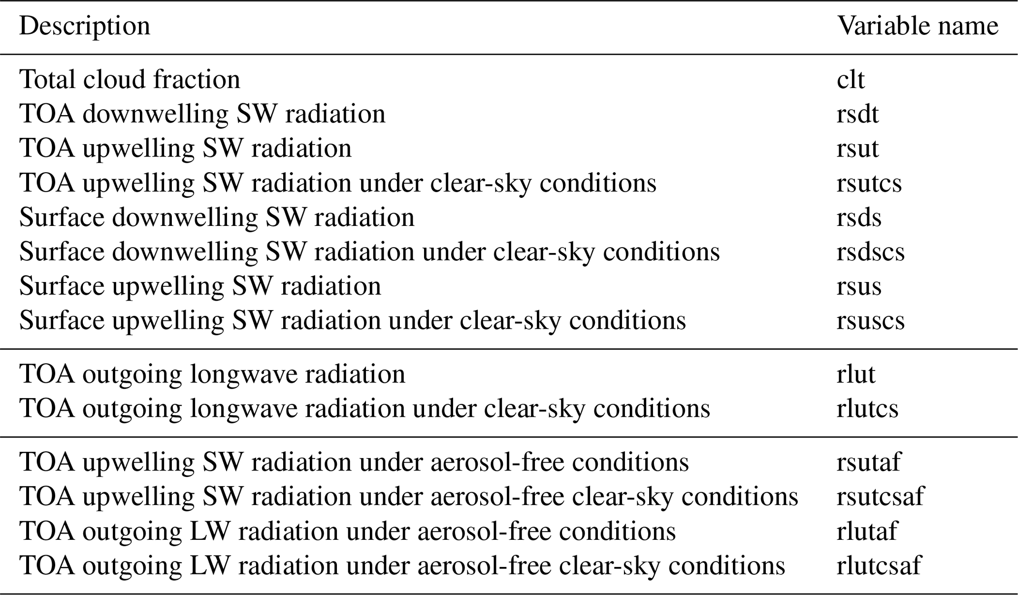
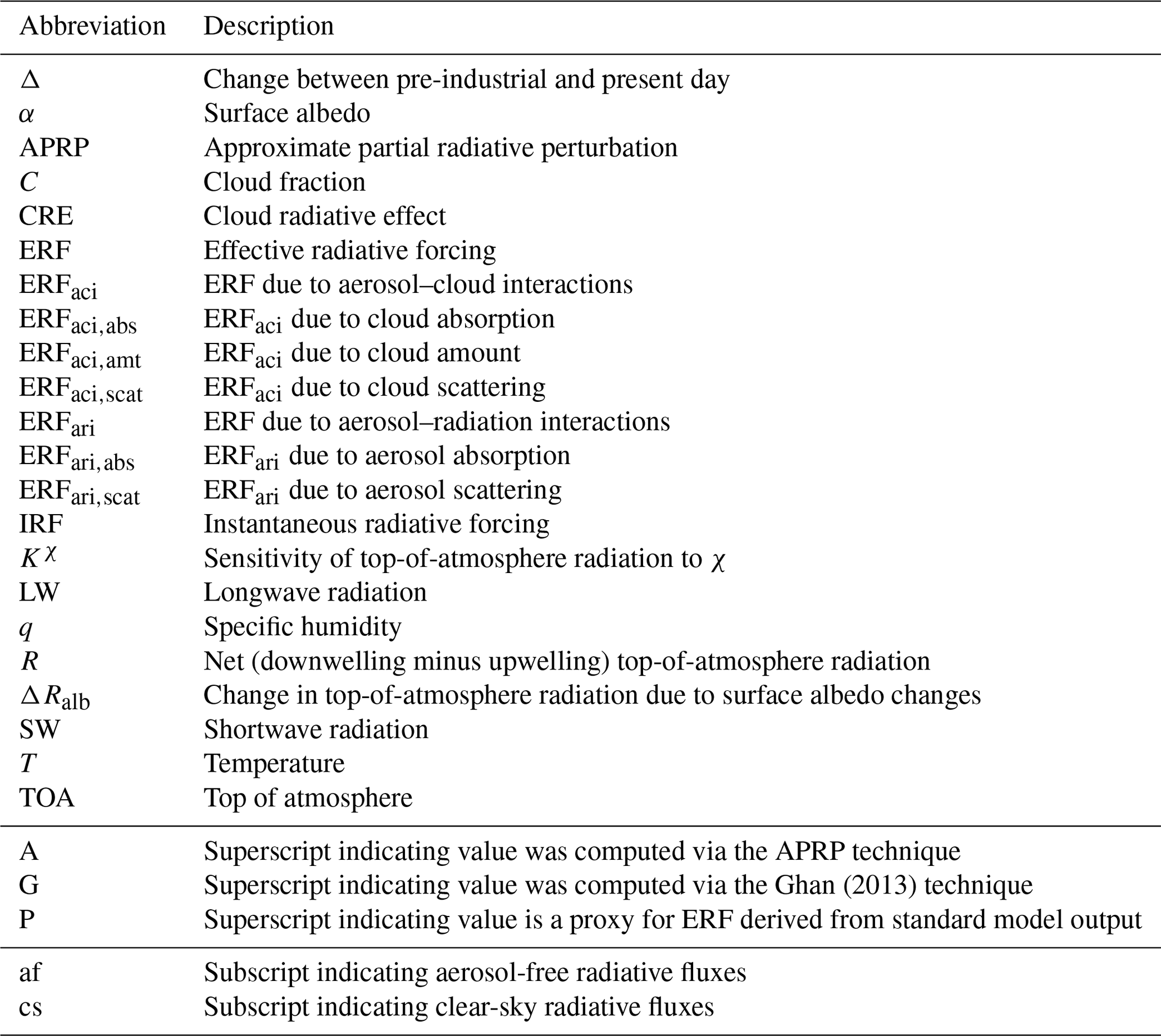
We make use of all available ensemble members of all models that performed these simulations (listed in Tables 1 and 2), with the exception of the EC-Earth3 model. This was excluded because of spurious up- and downwelling clear-sky shortwave radiative fluxes at the surface (“rsuscs” and “rsdscs”) that are determined to be erroneous and bias the APRP calculations. In particular, we identified numerous examples in which these fluxes exhibited very large values at individual grid cells and months but were surrounded in time and space by near-zero values (e.g., in winter locations with negligible insolation). The monthly fields used in our analyses are listed in Table A1, and abbreviations and other nomenclature used throughout the paper are listed in Table A2.

2.2 Aerosol effective radiative forcing calculations

2.2.1 IPCC AR6 definitions

One can express the total change in net (downwelling minus upwelling) radiation (ΔR) between a control experiment and an aerosol-perturbed experiment (both with fixed SSTs and SICs) as the sum of effective radiative forcings due to aerosol–radiation interactions (ERF_ari) and aerosol–cloud interactions (ERF_aci), as well as changes in top-of-atmosphere (TOA) radiation due to changes in surface albedo (ΔR_alb) and surface temperature ($\mathrm{\Delta }{R}_{T_{\mathrm{0}}}$):

$$\begin{array}{}\text{(1)}& \mathrm{\Delta }R={\mathrm{ERF}}_{\mathrm{ari}}+{\mathrm{ERF}}_{\mathrm{aci}}+\mathrm{\Delta }{R}_{\mathrm{alb}}+\mathrm{\Delta }{R}_{T_{\mathrm{0}}}.\end{array}$$

As defined in IPCC AR6 (Forster et al., 2021), ERF_ari comprises the instantaneous radiative forcing (IRF_ari), non-cloud atmospheric adjustments that are uncoupled to any change in global surface temperature, and adjustments of clouds due to changes in the thermal structure of the atmosphere caused by absorbing aerosols (also known as the “semidirect effect”):

$$\begin{array}{}\text{(2)}& {\mathrm{ERF}}_{\mathrm{ari}}={\mathrm{IRF}}_{\mathrm{ari}}+K^T\mathrm{\Delta }T+K^q\mathrm{\Delta }q+K^C\mathrm{\Delta }{C}_{\mathrm{semidirect}},\end{array}$$

where K^χ terms quantify the sensitivity of TOA net radiation to infinitesimal perturbations in variable χ,

$$\begin{array}{}\text{(3)}& K^{\mathit{\chi }}={\displaystyle \frac{\partial R}{\partial \mathit{\chi }}},\end{array}$$

and here and elsewhere χ may represent temperature (T), humidity (q), surface albedo (α), or clouds (C). It is intended that ΔT and Δq include only changes in tropospheric temperature and water vapor that occur independently of changes in surface temperature – not those that occur in response to any land surface temperature change in these fixed-SST simulations. In practice it is difficult to determine which portion of the change in any field is an adjustment to aerosols versus a response that is mediated by land surface temperature changes or by circulation changes induced by said temperature changes. Hence for simplicity we follow a conservative approach, also taken by AR6, and exclude the radiative impact of land temperature changes from ERF_ari. This approach leads to positive longwave ERF_ari values that are smaller than if this correction is not applied, making the overall net negative ERF about 5 % stronger on average across models, consistent with the 5 % inflation that IPCC AR6 applied to the ERF values derived in Smith et al. (2020) and Zelinka et al. (2014). Finally, the radiative impact of surface albedo changes – which we also keep separate from the ERF terms in Eq. (1) – arises due to deposition of absorbing aerosol on snow and ice, changes in snow and ice cover arising from the aerosol-induced change in climate, and aerosol-induced changes in the relative amount of direct versus diffuse radiation reaching the surface.

As defined in IPCC AR6, ERF_aci comprises the instantaneous radiative forcing due to changes in cloud liquid and ice particle number concentrations and sizes (IRF_aci), as well as subsequent adjustments of cloud water and coverage (K^CΔC_adjustments):

$$\begin{array}{}\text{(4)}& {\mathrm{ERF}}_{\mathrm{aci}}={\mathrm{IRF}}_{\mathrm{aci}}+K^C\mathrm{\Delta }{C}_{\mathrm{adjustments}}.\end{array}$$

Although the above decomposition of direct and indirect forcings is employed by IPCC AR6 (Forster et al., 2021), in the Ghan (2013) and APRP methods described below, there is no way to separately quantify the three cloud-related terms – the semidirect effect which is considered part of ERF_ari, the instantaneous component due to changing particle number and size (the Twomey effect), and the subsequent adjustments. Instead, for these two methodologies, the cloud terms are combined into a single term that is included as part of the ERF_aci:

$$\begin{array}{}\text{(5)}& K^C\mathrm{\Delta }C={\mathrm{IRF}}_{\mathrm{aci}}+K^C\mathrm{\Delta }{C}_{\mathrm{adjustments}}+K^C\mathrm{\Delta }{C}_{\mathrm{semidirect}}.\end{array}$$

K^CΔC can be further broken down into contributions from changes in cloud amount and optical properties.

2.2.2 Approximate partial radiative perturbation (APRP) technique

Taylor et al. (2007) developed an efficient method of decomposing perturbations to the TOA SW energy budget from clouds, the cloud-free portion of the atmosphere (here assumed to be dominated by aerosols), and surface albedo. Briefly, the APRP method employs a simple one-layer model of the atmosphere to diagnose the scattering and absorption of SW radiation at the surface and in the atmosphere. This simple model represents the transfer of SW radiation through the atmosphere at every grid point on the globe in terms of a small number of parameters – the insolation, surface albedo, an atmospheric scattering coefficient, and an atmospheric absorptance coefficient. Given the known SW fluxes at the TOA and surface under both clear- and all-sky conditions as well as the total cloud fraction, at each grid point on the globe one can solve for the atmospheric scattering and absorption parameters in this simplified representation such that the upwelling and downwelling SW radiative fluxes at the surface and TOA match those produced by the global climate model (GCM). Then the sensitivity of TOA albedo to these parameters can be determined, allowing one to isolate the individual contributions from changes in non-cloud atmospheric constituents and from changes in cloud properties. This technique is an approximation to the more rigorous but difficult-to-implement partial radiative perturbation (PRP) technique, and it was shown to closely agree with PRP-derived SW cloud and surface albedo feedbacks (Taylor et al., 2007), with errors that were no larger than 10 %. It is uniquely well suited for quantifying and decomposing aerosol forcing, since aerosols primarily affect scattering and absorption of SW radiation both directly and indirectly through clouds. A more detailed description of APRP and how it is used to estimate the individual aerosol forcing components is provided in Appendix A2, and code to perform all APRP calculations for this paper is provided in the “Code availability” section.

APRP (denoted below with a superscript A) provides estimates of SW ERF (superscript SW) that are made up of slightly different term groupings than the IPCC AR6 definition:

$$\begin{array}{}\text{(6)}& \begin{array}{rl}{\mathrm{ERF}}_{\mathrm{ari}}^{\mathrm{A},\mathrm{SW}}& ={\mathrm{IRF}}_{\mathrm{ari}}^{\mathrm{SW}}+K^{q,\mathrm{SW}}\mathrm{\Delta }q\\ & ={\mathrm{ERF}}_{\mathrm{ari}}^{\mathrm{SW}}-K^{C,\mathrm{SW}}\mathrm{\Delta }{C}_{\mathrm{semidirect}}\end{array}\end{array}$$

and

$$\begin{array}{}\text{(7)}& \begin{array}{rl}{\mathrm{ERF}}_{\mathrm{aci}}^{\mathrm{A},\mathrm{SW}}& ={\mathrm{IRF}}_{\mathrm{aci}}^{\mathrm{SW}}+K^{C,\mathrm{SW}}\mathrm{\Delta }{C}_{\mathrm{adjustments}}+K^{C,\mathrm{SW}}\mathrm{\Delta }{C}_{\mathrm{semidirect}}\\ & ={\mathrm{ERF}}_{\mathrm{aci}}^{\mathrm{SW}}+K^{C,\mathrm{SW}}\mathrm{\Delta }{C}_{\mathrm{semidirect}}.\end{array}\end{array}$$

The impact of temperature changes on the SW ERF_ari can be neglected. Therefore in the SW, APRP's direct effect equals IPCC's direct effect minus the semidirect effect, while APRP's indirect effect equals IPCC's indirect effect plus the semidirect effect. The sum of the direct and indirect SW effects is the same, independent of how the individual components are defined. Thus, from Eqs. (6) and (7),

$$\begin{array}{}\text{(8)}& {\mathrm{ERF}}_{\mathrm{ari}}^{\mathrm{A},\mathrm{SW}}+{\mathrm{ERF}}_{\mathrm{aci}}^{\mathrm{A},\mathrm{SW}}={\mathrm{ERF}}_{\mathrm{ari}}^{\mathrm{SW}}+{\mathrm{ERF}}_{\mathrm{aci}}^{\mathrm{SW}}.\end{array}$$

Further insight comes from separating ERF${}_{\mathrm{ari}}^{\mathrm{A},\mathrm{SW}}$ into absorption and scattering components,

$$\begin{array}{}\text{(9)}& {\mathrm{ERF}}_{\mathrm{ari}}^{\mathrm{A},\mathrm{SW}}={\mathrm{ERF}}_{\mathrm{ari},\mathrm{abs}}^{\mathrm{A},\mathrm{SW}}+{\mathrm{ERF}}_{\mathrm{ari},\mathrm{scat}}^{\mathrm{A},\mathrm{SW}},\end{array}$$

and from separating ERF${}_{\mathrm{aci}}^{\mathrm{A},\mathrm{SW}}$ into cloud absorption, amount, and scattering components,

$$\begin{array}{}\text{(10)}& {\mathrm{ERF}}_{\mathrm{aci}}^{\mathrm{A},\mathrm{SW}}={\mathrm{ERF}}_{\mathrm{aci},\mathrm{abs}}^{\mathrm{A},\mathrm{SW}}+{\mathrm{ERF}}_{\mathrm{aci},\mathrm{amt}}^{\mathrm{A},\mathrm{SW}}+{\mathrm{ERF}}_{\mathrm{aci},\mathrm{scat}}^{\mathrm{A},\mathrm{SW}}.\end{array}$$

APRP also quantifies the impact of surface albedo changes on TOA SW radiation.

2.2.3 LW ERFs: proxies derived from standard model output

There is no equivalent to APRP for LW radiation, so instead we compute proxies (denoted with superscript P) for LW ERFs using standard model output, following Zelinka et al. (2014) and Smith et al. (2020). The LW direct effect is estimated as the change in clear-sky TOA LW radiation excluding the portion due solely to land surface temperature changes:

$$\begin{array}{}\text{(11)}& {\mathrm{ERF}}_{\mathrm{ari}}^{\mathrm{P},\mathrm{LW}}=\mathrm{\Delta }{R}_{\mathrm{cs}}^{\mathrm{LW}}-\mathrm{\Delta }{R}_{\mathrm{cs}}^{T_{\mathrm{0}}},\end{array}$$

where R^LW refers to net (downwelling minus upwelling) LW radiation and the subscript “cs” refers to clear-sky conditions. The change in clear-sky LW radiation due to changes in (land) surface temperature is computed by multiplying the change in surface temperature between the two experiments by the clear-sky surface temperature radiative kernel (Huang et al., 2017):

$$\begin{array}{}\text{(12)}& \mathrm{\Delta }{R}_{\mathrm{cs}}^{T_{\mathrm{0}}}=K_{\mathrm{cs}}^{T_{\mathrm{0}}}\mathrm{\Delta }{T}_{\mathrm{0}}.\end{array}$$

We compute a proxy for longwave ERF_aci as the change in LW cloud radiative effect:

$$\begin{array}{}\text{(13)}& {\mathrm{ERF}}_{\mathrm{aci}}^{\mathrm{P},\mathrm{LW}}=\mathrm{\Delta }{\mathrm{CRE}}^{\mathrm{LW}}=\mathrm{\Delta }{R}^{\mathrm{LW}}-\mathrm{\Delta }{R}_{\mathrm{cs}}^{\mathrm{LW}}.\end{array}$$

As shown in Appendix B, our proxy for the LW direct effect equals IPCC's direct effect minus the semidirect effect minus masking terms that quantify how much the radiative impact of changes in temperature, humidity, and aerosols is attenuated by the presence of clouds. Our proxy for the LW indirect effect equals IPCC's indirect effect plus the semidirect effect plus the aforementioned masking terms.

2.2.4 Double-radiation-call method

Ghan (2013) introduced a method to compute aerosol direct and indirect effects that relies on aerosol-free radiative fluxes under both clear- and all-sky conditions. These are produced by performing additional calls to the radiation code during model integration in which all aerosols are neglected. For the models that provide aerosol-free radiative fluxes, we compute the following quantities, which are given the superscript G to indicate Ghan. Ghan (2013) defines the direct forcing as

$$\begin{array}{}\text{(14)}& {\mathrm{ERF}}_{\mathrm{ari}}^{\mathrm{G}}=\mathrm{\Delta }R-\mathrm{\Delta }{R}_{\mathrm{af}},\end{array}$$

the indirect forcing as

$$\begin{array}{}\text{(15)}& {\mathrm{ERF}}_{\mathrm{aci}}^{\mathrm{G}}=\mathrm{\Delta }{R}_{\mathrm{af}}-\mathrm{\Delta }{R}_{\mathrm{af},\mathrm{cs}},\end{array}$$

and a third forcing term as

$$\begin{array}{}\text{(16)}& {\mathrm{ERF}}_{\mathrm{other}}^{\mathrm{G}}=\mathrm{\Delta }{R}_{\mathrm{af},\mathrm{cs}}.\end{array}$$

where the subscript “af” refers to aerosol-free radiative fluxes and, as above, ΔR represents the change in net radiation between the control and aerosol-perturbed experiment.

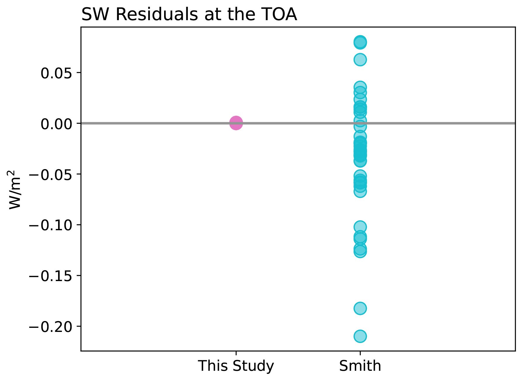
Figure 1 Global mean residuals estimated as the difference between the model-produced change in TOA SW fluxes and those estimated by summing the APRP components, shown for the APRP implementation in this study and in Smith et al. (2020). Each marker represents a different CMIP model (all pink markers overlap).

As shown in Appendix B, Ghan's direct aerosol radiative forcing equals IPCC's instantaneous direct forcing minus masking terms that quantify how much the radiative impact of changes in temperature, humidity, surface albedo, and clouds is attenuated by the presence of aerosols. Ghan's indirect effect equals IPCC's indirect effect plus masking terms that quantify how much the radiative impact of changes in temperature, humidity, and surface albedo is attenuated by the presence of clouds under aerosol-free conditions and how much the radiative impact of changes in clouds is attenuated by the presence of aerosols plus the semidirect effect. Finally, ${\mathrm{ERF}}_{\mathrm{other}}^{\mathrm{G}}$ – which in the SW Ghan (2013) refers to as the surface albedo forcing – equals ΔR_alb plus the aerosol-free clear-sky radiative contributions from changes in humidity plus a masking term that quantifies how much the radiative impact of changes in surface albedo is attenuated by the presence of both clouds and aerosols.

3 Results

3.1 Errors in APRP implementation of Smith et al. (2020)

We begin by comparing the sum of all APRP-derived SW ERF components with the total change in SW radiation between the perturbed aerosol and control experiment. Since the majority of the results shown below are derived using APRP, we omit the A superscript hereafter. If APRP is correctly implemented, the sum of its components should perfectly reproduce the total change in SW radiation between the control and perturbed experiment. As shown in Fig. 1, the APRP implementation in the present study has a negligible residual, whereas that in Smith et al. (2020) is generally nonzero, ranging from −0.21 to +0.08 W m⁻² across models. These errors, resulting from a mistake in coding as detailed below, are comparable in magnitude to typical values for the total aerosol direct effect and the cloud absorption and amount components of the indirect effect (shown below).

The small residual in Smith's implementation of APRP masks the two much larger errors that are nearly perfectly compensating. The first error – which in isolation leads to overestimated ERF magnitudes – is in how TOA albedo sensitivities are computed, particularly in the calculation of overcast-sky albedo sensitivity to aerosol and cloud absorption and scattering. The code overestimated the impact of changes in scattering or absorption on overcast-sky fluxes because it made use of the raw difference between clear-sky scattering and absorption coefficients. The correct implementation, in contrast, scales this difference by the appropriate factor to account for the fact that changes in the non-cloud portion of a column are attenuated by the presence of clouds in the column. This error is described in further detail in Appendix A3. The second error – which in isolation leads to underestimated ERF magnitudes – is that net (downwelling minus upwelling) rather than downwelling TOA SW radiation was used in all calculations. This error is described in further detail in Appendix A4.

To quantify the impact of these two errors, we first corrected both errors in the code of Smith et al. (2020) and verified that it produces results identical to those from the original APRP implementation of Zelinka et al. (2014). The correct implementation is shown as pink bars in Fig. 2 and serves as the baseline against which subsequent calculations are compared. We then performed the APRP calculations two more times: once reverting back to the original erroneous insolation formulation and once reverting back to the original erroneous albedo sensitivity formulation. The ERF estimate derived from the APRP implementation with erroneous insolation is shown by the dotted hatching overlain on the pink bar. This bar has a smaller magnitude than the true value because it uses net (downwelling minus upwelling radiation) rather than downwelling radiation. The ratio of these two ERF estimates (shown in printed numbers) is 0.77 averaged across models, with a standard deviation of 0.05. This is consistent with the fact that net radiation is equal to the downwelling radiation times (1 minus planetary albedo) and that planetary albedos vary between about 0.2 and 0.3.

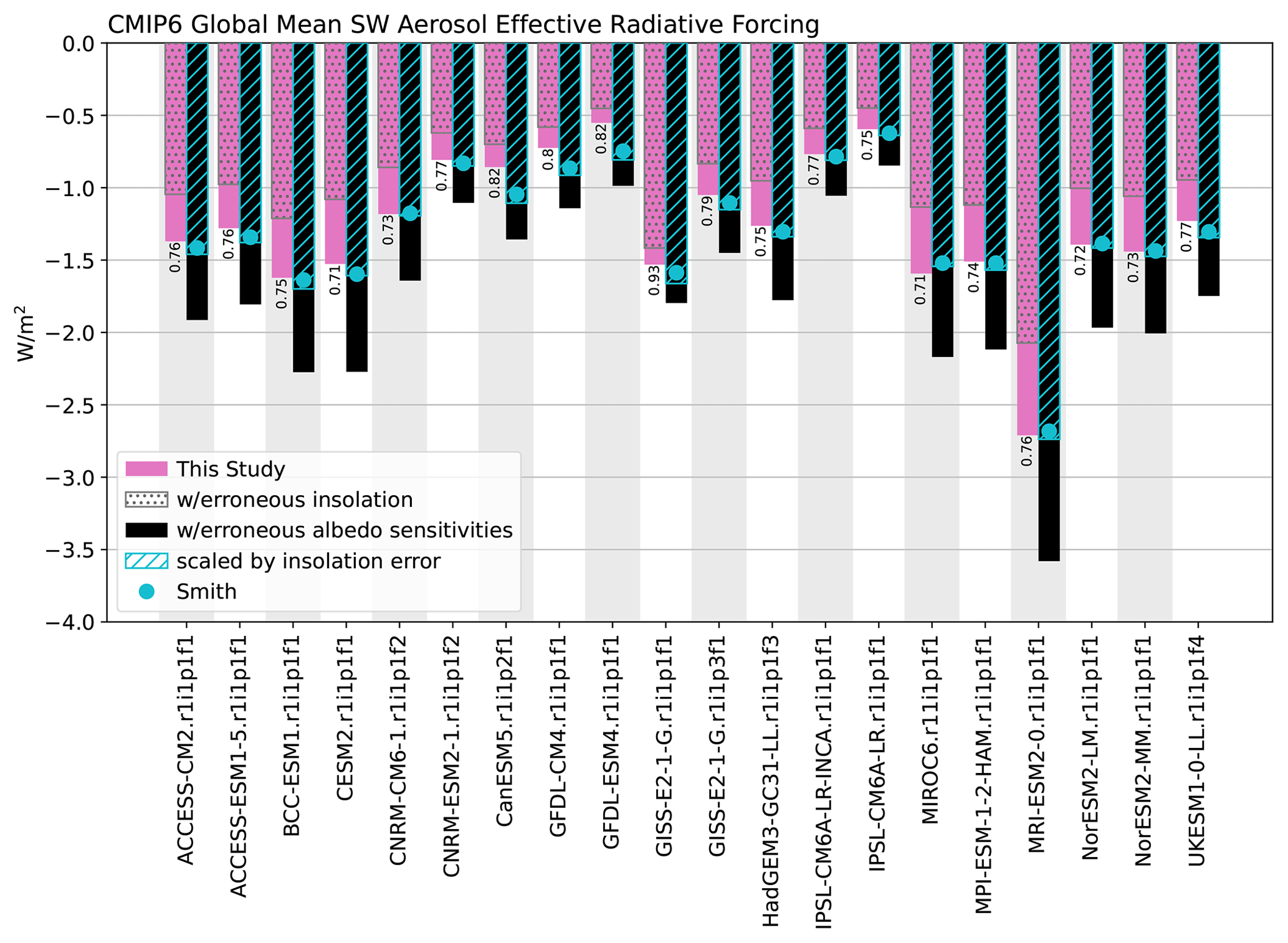
Figure 2 Estimates of global mean ERF${}_{\mathrm{ari}+\mathrm{aci}}^{\mathrm{SW}}$ across CMIP6 models. The pink bar shows the values derived in this study using the corrected APRP formulation. Overlain on this with dotted gray hatching is the ERF derived if using net rather than downwelling SW radiation, and the ratio between these two is printed. The adjacent black bar shows the ERF derived if using erroneous albedo sensitivities (but correct insolation). Overlain on this with cyan hatching is this same value scaled by the aforementioned ratio, which closely matches the values derived using the APRP formulation of Smith et al. (2020), which are shown with cyan dots.

The ERF estimates derived from the APRP implementation with erroneous albedo sensitivities (but correct insolation) are shown in the black bars in Fig. 2. The erroneous albedo sensitivity formulation leads to ERF values that are biased too large in magnitude. This arises almost entirely from the scattering components of ERF${}_{\mathrm{aci}}^{\mathrm{SW}}$ and ERF${}_{\mathrm{ari}}^{\mathrm{SW}}$, which are overestimated (discussed further below). This occurs because the erroneous code did not properly allow the increase in aerosol scattering to be attenuated by cloud scattering and did not properly allow the increase in cloud scattering to be attenuated by non-cloud (aerosol) scattering (not shown).

The bar with cyan hatching overlain on the black bar in Fig. 2 indicates the result if we scale these overestimated ERFs by the ratios diagnosed above to account for the compensating insolation error. This scaled estimate closely matches the original Smith et al. (2020) formulation in which both errors are present (cyan dots).

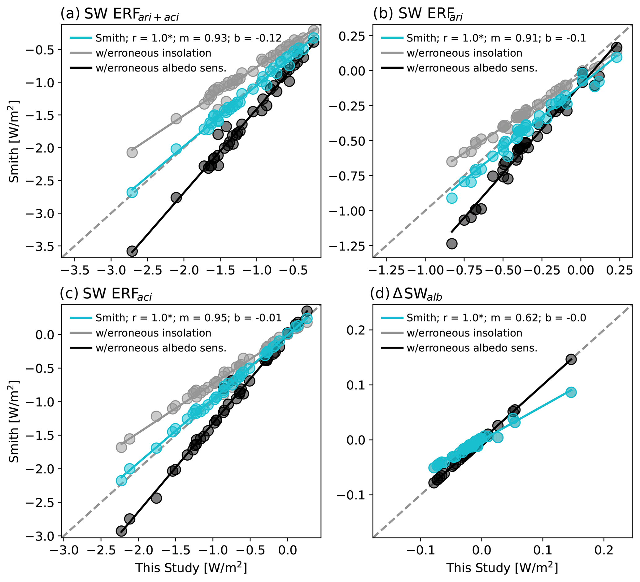
Figure 3 Estimates of global mean (a) ERF${}_{\mathrm{ari}+\mathrm{aci}}^{\mathrm{SW}}$, (b) ERF${}_{\mathrm{ari}}^{\mathrm{SW}}$, (c) ERF${}_{\mathrm{aci}}^{\mathrm{SW}}$, and (d) ΔSW_alb in each CMIP5 and CMIP6 model derived using the APRP formulation of Smith et al. (2020) scattered against estimates computed in this study. Cyan markers indicate the values estimated by Smith et al. (2020), gray markers indicate values derived using net rather than downwelling SW radiation (but correct albedo sensitivities), and black markers indicate values derived using erroneous albedo sensitivities (but correct insolation). Gray markers in panel (d) are overlain by cyan markers. Correlation, slope, and intercept are reported as r, m, and b, respectively, and correlations that are statistically significant at 95 % confidence are indicated with an asterisk.

Hence the two errors are individually substantial in magnitude but act in opposite directions that almost perfectly compensate, leading to total ERF values that are in good agreement with the correct values estimated here using the APRP implementation of Zelinka et al. (2014). This also holds for the geographic structure of the ERF components, which are highly consistent between the two APRP implementations but differ quantitatively (not shown). This appears to be a fortuitous result. Moreover, while this good agreement with the correct values holds for the total ERF, several of its sub-components show larger biases, as discussed next.

In Fig. 3 we scatter estimates of ERF${}_{\mathrm{ari}+\mathrm{aci}}^{\mathrm{SW}}$, its two sub-components (ERF${}_{\mathrm{ari}}^{\mathrm{SW}}$ and ERF${}_{\mathrm{aci}}^{\mathrm{SW}}$), and the ΔSW_alb term derived using the APRP implementation of Smith et al. (2020) against those derived using the implementation of Zelinka et al. (2014). ERF${}_{\mathrm{ari}}^{\mathrm{SW}}$ and ERF${}_{\mathrm{aci}}^{\mathrm{SW}}$ are further broken down into their scattering and absorption sub-components in Fig. 4. The aforementioned compensating biases are indicated by the gray and black markers, which show the ERF values derived if correcting each bias in turn. Correcting the albedo sensitivity formulation but keeping the insolation bias leads to ERF values that are too small in magnitude (Figs. 3–4, gray markers). This is expected because a given change in albedo will produce a weaker TOA impact when using a smaller (downwelling minus upwelling) SW radiation stream. Further details are provided in Appendix A4.

Figure 4 As in Fig. 3 but for the scattering and absorption sub-components of ERF${}_{\mathrm{ari}}^{\mathrm{SW}}$ and ERF${}_{\mathrm{aci}}^{\mathrm{SW}}$.

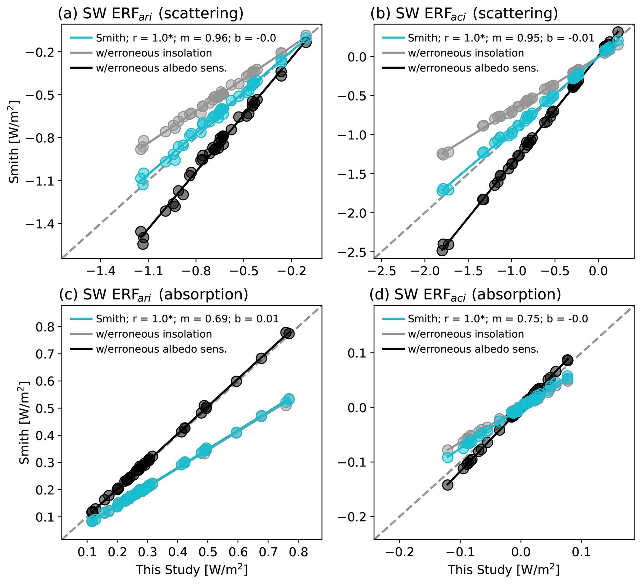
Correcting the insolation but keeping the erroneous albedo sensitivity formulation (black markers) has the opposite effect: in most cases it leads to ERF values that are too large in magnitude for reasons described in Appendix A3. This indicates that using correct values of downwelling (rather than net) SW radiation exposes the erroneous albedo sensitivity formulation wherein changes in scattering or absorption have too-strong an effect on TOA SW radiation. This error primarily manifests itself in the scattering components of ERF${}_{\mathrm{ari}}^{\mathrm{SW}}$ and ERF${}_{\mathrm{aci}}^{\mathrm{SW}}$ (Fig. 4a and b, black markers), whereas the absorption components are largely corrected when the insolation is corrected (Fig. 4c and d, black markers). The albedo sensitivity formulation error has a larger impact on the scattering components because clouds scatter more SW radiation than they absorb. This means that neglecting the attenuation of the change in aerosol scattering by cloud scattering induces a larger error than neglecting cloud absorption when computing the impact of a change in aerosol absorption. Finally, the ΔSW_alb bias vanishes once the insolation bias is corrected (Fig. 3d, black markers). This is because, unlike for the sensitivity of planetary albedo to atmospheric scattering and absorption parameters, the sensitivity of planetary albedo to surface albedo is implemented correctly in Smith et al. (2020).

For the ERF components that depend only on scattering of radiation, these two biases largely compensate such that the values reported in Smith et al. (2020) agree well with those estimated here (Fig. 4a and b, cyan markers). However, for the absorption components of ERF${}_{\mathrm{ari}}^{\mathrm{SW}}$ and ERF${}_{\mathrm{aci}}^{\mathrm{SW}}$ (for which the albedo sensitivity formulation was not as biased) and for the surface albedo term (which does not depend on how the atmospheric scattering and absorption sensitivities are formulated), the insolation error is largely uncompensated. Therefore, the values reported in Smith et al. (2020) remain systematically biased for these components. This is most apparent for ΔSW_alb (Fig. 3d) and the absorption component of ERF${}_{\mathrm{ari}}^{\mathrm{SW}}$ (Fig. 4c).

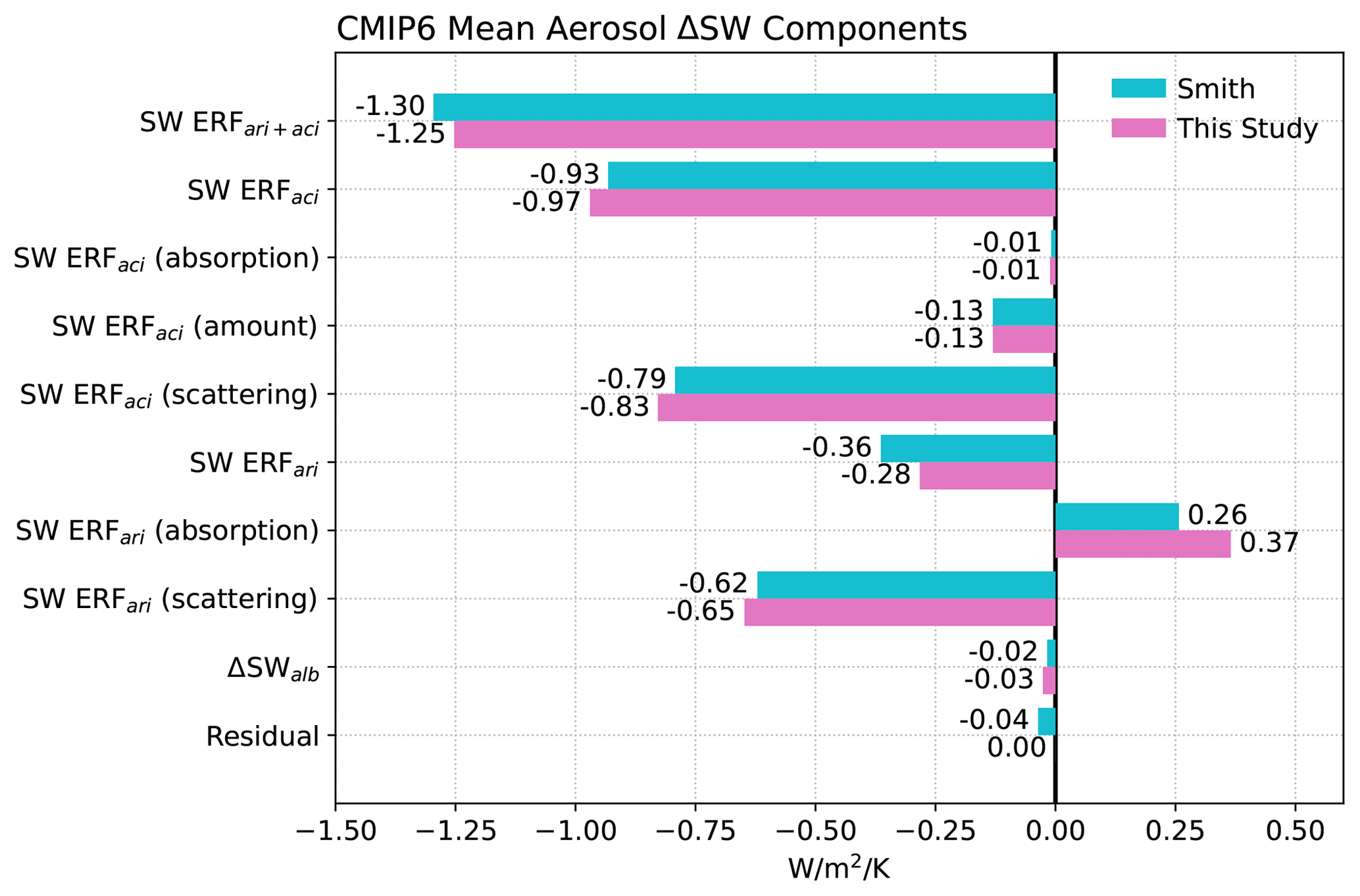
Figure 5 Components of the change in global mean SW TOA radiation averaged across CMIP6 models as computed by Smith et al. (2020) and as computed in this study.

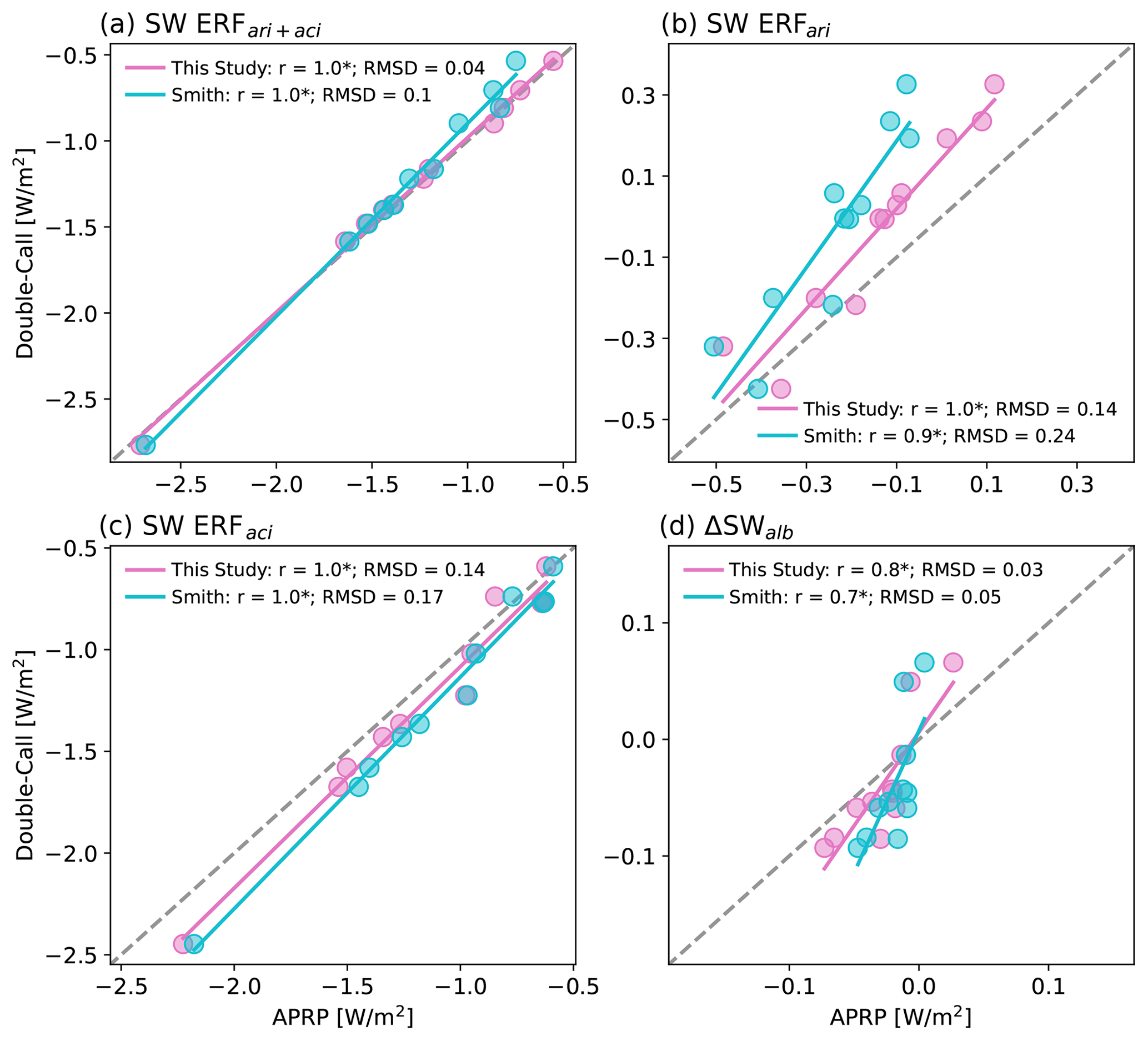
Figure 6 Estimates of global mean (a) ERF${}_{\mathrm{ari}+\mathrm{aci}}^{\mathrm{SW}}$, (b) ERF${}_{\mathrm{ari}}^{\mathrm{SW}}$, (c) ERF${}_{\mathrm{aci}}^{\mathrm{SW}}$, and (d) ΔSW_alb derived using the APRP method as implemented in this study (pink) and in Smith et al. (2020) (blue) in each CMIP6 model scattered against estimates computed using the double-call method of Ghan (2013). Note that we are referring to Ghan's ERF${}_{\mathrm{other}}^{\mathrm{SW}}$ as ΔSW_alb here even though the former receives contributions from more than just changes in surface albedo (see Appendix B). The correlation and root-mean-square difference are reported as r and RMSD, respectively, and correlations that are statistically significant at 95 % confidence are indicated with an asterisk.

Figure 5 shows the CMIP6 multi-model mean SW ERF components estimated using the APRP formulation of Smith et al. (2020) and as derived in this study. Note that the Smith et al. values differ slightly from those reported in that study because here we include four additional CMIP6 models not assessed in that study and exclude EC-Earth3, which was used in that study. We find that all but three ERF values are within 5 % of those diagnosed by Smith et al. (2020): The very small ΔSW_alb component increases in strength from −0.02 to −0.03 W m⁻². More importantly, the negative ERF${}_{\mathrm{ari}}^{\mathrm{SW}}$ diagnosed here is roughly 20 % weaker in magnitude. This is primarily because the positive absorbing component of ERF${}_{\mathrm{ari}}^{\mathrm{SW}}$ is roughly 40 % larger in the present study.

3.2 Validation of ERF estimates against the double-call method

In Fig. 6 we compare the SW ERF values estimated using APRP with those derived using the technique of Ghan (2013) in which radiation calculations are performed an additional time with all aerosols neglected. This comparison is done for 10 models (indicated with asterisks in Table 2) that provided the necessary aerosol-free diagnostics. As mentioned earlier and as detailed in Appendix B, APRP and Ghan (2013) define each of these terms differently, so differences between the two estimates do not necessarily indicate errors. However, one would expect these to be closely related, and, when implemented correctly, APRP values closely reproduce the double-call values. Indeed, both APRP implementations are well correlated with the double-call method for each ERF component, but the root-mean-square-deviation (RMSD) values are much smaller when using the values derived in this study.

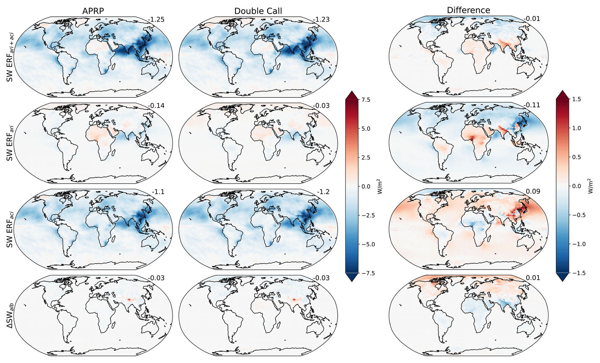
Figure 7 ERF${}_{\mathrm{ari}+\mathrm{aci}}^{\mathrm{SW}}$ (row 1), ERF${}_{\mathrm{ari}}^{\mathrm{SW}}$ (row 2), ERF${}_{\mathrm{aci}}^{\mathrm{SW}}$ (row 3), and ΔSW_alb (row 4) estimated by the APRP method (column 1), the double-call method (column 2), and their difference (column 3). Area-weighted global mean values are printed in the top-right corner of each panel. Results are averaged across all models providing double-call output.

Even when correctly implemented, APRP-estimated ERF${}_{\mathrm{ari}}^{\mathrm{SW}}$ values are biased towards stronger negative/weaker positive values than those derived via double call (Fig. 6b). This is compensated somewhat by the ERF${}_{\mathrm{aci}}^{\mathrm{SW}}$ values, for which the APRP method is biased towards smaller negative values (Fig. 6c), as also shown for a single model in Zelinka et al. (2014). APRP also yields ΔSW_alb values that are weaker in magnitude than produced by the double call (Fig. 6d). As shown in Appendix B, these differences are expected because the two methods are diagnosing slightly different things for each of the individual components, with the offset arising from small masking terms. For example, Ghan (2013) defines ΔSW_alb as the change in clear-sky aerosol-free SW fluxes (Eq. 16), whereas the APRP quantifies this as the change in all-sky radiation due to changes in surface albedo. Hence the latter calculation allows the radiative impact of changing surface albedo to be attenuated by the presence of clouds and aerosols (i.e., masking effects) and avoids aliasing in contributions from humidity changes that impact SW absorption. Indeed, the double-call ΔSW_alb values agree closely with the clear-sky surface albedo component diagnosed by APRP scaled by the clear-sky fraction (r=1.0; RMSD = 0.02; not shown).

The multi-model mean maps show excellent agreement in the spatial structure of each component between the correct implementation of APRP and Ghan (2013) methodologies, albeit with quantitative differences (Fig. 7). Both methods agree on negative ERF${}_{\mathrm{ari}+\mathrm{aci}}^{\mathrm{SW}}$ over the vast majority of the Northern Hemisphere, with the largest negative values over the northern Indian Ocean and over Southeast Asia. Negative values are also present across the North Pacific and North Atlantic oceans and over most of the Northern Hemisphere continental regions, and local maxima are present just west of South America and Africa.

Both methods diagnose a positive ERF${}_{\mathrm{ari}}^{\mathrm{SW}}$ over Africa (Fig. 7, row 2). The APRP results indicate that this is a region of strong aerosol absorption that is not fully countered by aerosol scattering (not shown), perhaps indicating a role of black carbon from biomass burning. Just east of this, the two methods agree on a negative direct effect over the northern Indian Ocean. Despite the large aerosol emission sources, the ERF${}_{\mathrm{ari}}^{\mathrm{SW}}$ is not particularly large over Southeast Asia because of close compensation between the absorbing and scattering components (not shown). The spatial structure of the total ERF is very consistent with the ERF${}_{\mathrm{aci}}^{\mathrm{SW}}$ map (Fig. 7, row 3), highlighting the dominant role played by the indirect effect in models' total aerosol forcing. Weak negative ΔSW_alb values are present over much of the NH continents, likely due to increased snow cover in response to aerosol-induced cooling (Fig. 7, row 4). An exception is a region of large positive ΔSW_alb over the Himalayas, which may result from black carbon deposition on snow.

Consistent with the comparison for a single model shown in Zelinka et al. (2014), locations where APRP overestimates the negative ERF${}_{\mathrm{ari}}^{\mathrm{SW}}$ are co-located with locations where it underestimates ERF${}_{\mathrm{aci}}^{\mathrm{SW}}$, and vice versa. This is noticeable over the North Pacific Ocean downwind of the eastern Asia ERF${}_{\mathrm{ari}+\mathrm{aci}}^{\mathrm{SW}}$ maximum. These opposite-signed differences with respect to the double-call method cancel such that the total ERF${}_{\mathrm{ari}+\mathrm{aci}}^{\mathrm{SW}}$ maps are nearly identical (Fig. 7, row 1). The global mean root-mean-square difference between APRP and double-call estimates of ERF${}_{\mathrm{ari}+\mathrm{aci}}^{\mathrm{SW}}$ is less than 10 % of the standard deviation of either field, confirming that both methods agree as to spatial variations.

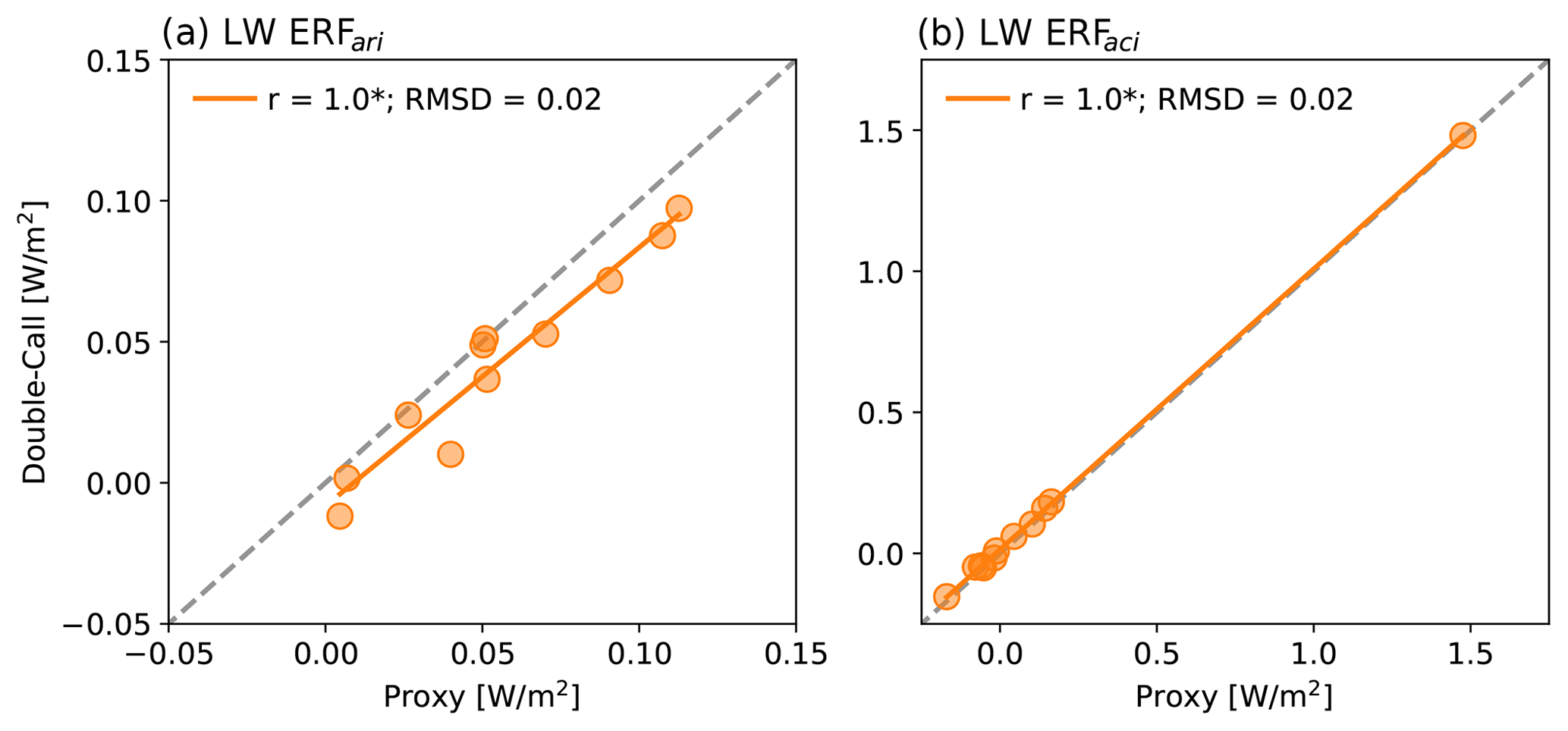
Figure 8 Estimates of global mean (a) ERF${}_{\mathrm{ari}}^{\mathrm{LW}}$ and (b) ERF${}_{\mathrm{aci}}^{\mathrm{LW}}$ derived using standard output from each CMIP6 model scattered against estimates computed using the double-call method of Ghan (2013). The double-call estimate in panel (a) is the sum of ERF${}_{\mathrm{ari}}^{\mathrm{G},\mathrm{LW}}$ and ERF${}_{\mathrm{other}}^{\mathrm{G},\mathrm{LW}}$ with the surface temperature response removed (see Appendix B).

Longwave ERF components cannot be derived using APRP, but we can derive proxies for the direct and indirect components from standard model output (Sect. 2.2.3). Specifically, we use the change in clear-sky LW radiation with the contribution from changes in surface temperature removed as a proxy for the LW direct effect. Recall that the formulation of Ghan (2013) defines the direct effect as the difference between changes in LW radiation under aerosol-free conditions and under all-sky conditions (Eq. 14). As demonstrated mathematically in Appendix B and as shown in Fig. 8a, our ${\mathrm{ERF}}_{\mathrm{ari}}^{\mathrm{LW}}$ proxy is closely related to the sum of Ghan's ERF${}_{\mathrm{ari}}^{\mathrm{LW},\mathrm{G}}$ and ERF${}_{\mathrm{other}}^{\mathrm{LW},\mathrm{G}}$ terms with the contribution from changes in surface temperature removed. In other words, the change in clear-sky LW radiation is made up of the direct aerosol effect as defined in Ghan (2013) plus perturbations due to aerosol-induced fast adjustments of humidity and temperature, including at the surface.

The change in LW cloud radiative effect (CRE) – our proxy for the LW indirect effect – is very well correlated with ERF${}_{\mathrm{aci}}^{\mathrm{LW}}$ derived with the double-call method (Fig. 8b), justifying its use as a proxy for the LW indirect effect. The model with large ERF${}_{\mathrm{aci}}^{\mathrm{LW}}$ apparent in Fig. 8b is MRI-ESM2-0, whose CMIP5-era counterpart also exhibited a large indirect component in the LW. This model was among only a few in CMIP5 that parameterized aerosol impacts on ice clouds, and it exhibited large changes in the amount and optical depth of high clouds in response to aerosols (Zelinka et al., 2014). This remains the model with largest aerosol effects on high clouds and therefore on LW cloud radiative fluxes, as discussed further in Smith et al. (2020).

We conclude from this section that the APRP technique yields aerosol ERF values that agree well with the independent double-call method, both in the global average and in the spatial distribution. Given that it does not require advanced diagnostics that may not be available in many models and experiments, it is an attractive method for systematically diagnosing these values across a broad suite of climate models. The typically smaller LW components of aerosol forcing are likewise well captured using simpler diagnostics that are widely available.

3.3 Summary of corrected APRP-derived ERF values

Having established that biases were present in the values of aerosol ERF provided in Smith et al. (2020) and that the values derived herein have negligible residuals and are in better agreement with the double-call method, we now provide the aerosol ERF values for all available models, along with their breakdown into components (Tables 1–2). This includes several CMIP6 models that were not available at the time Smith et al. (2020) was published. Although our APRP implementation is unchanged from that used in Zelinka et al. (2014), we report here CMIP5 results that include three additional models (bcc-csm1-1, FGOALS-s2, and MPI-ESM-LR) that were not included in the earlier paper.

Table 1 Aerosol ERF_ari, ERF_aci, and ERF_ari+aci values [W m⁻²] estimated for individual CMIP5 models, separated into SW, LW, and net components. The ERF${}_{\mathrm{ari}}^{\mathrm{SW}}$ is further separated into scattering and absorption components, and the ERF${}_{\mathrm{aci}}^{\mathrm{SW}}$ is further separated into scattering, absorption, and amount components. Also shown are the multi-model means and across-model standard deviations, both computed using only one ensemble member per model. Forcings are for present day (year 2000) relative to pre-industrial conditions.

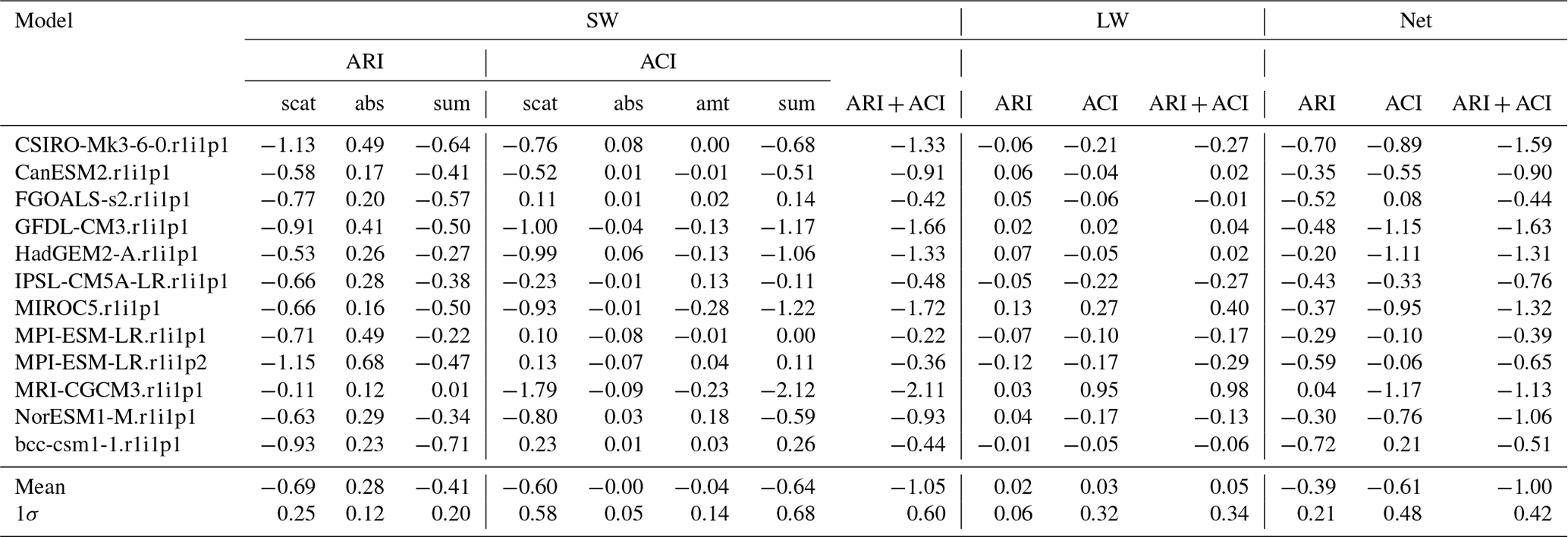
Table 2 As in Table 1 but for CMIP6 models. Models that provided aerosol-free diagnostics (allowing for the comparisons in Figs. 6–8) are indicated with asterisks. Multi-model means and across-model standard deviations are computed using only one ensemble member per model, but we treat the r1i1p1f1 and r1i1p3f1 members of GISS-E2-1-G as separate models. Forcings are for present day (year 2014) relative to pre-industrial conditions.

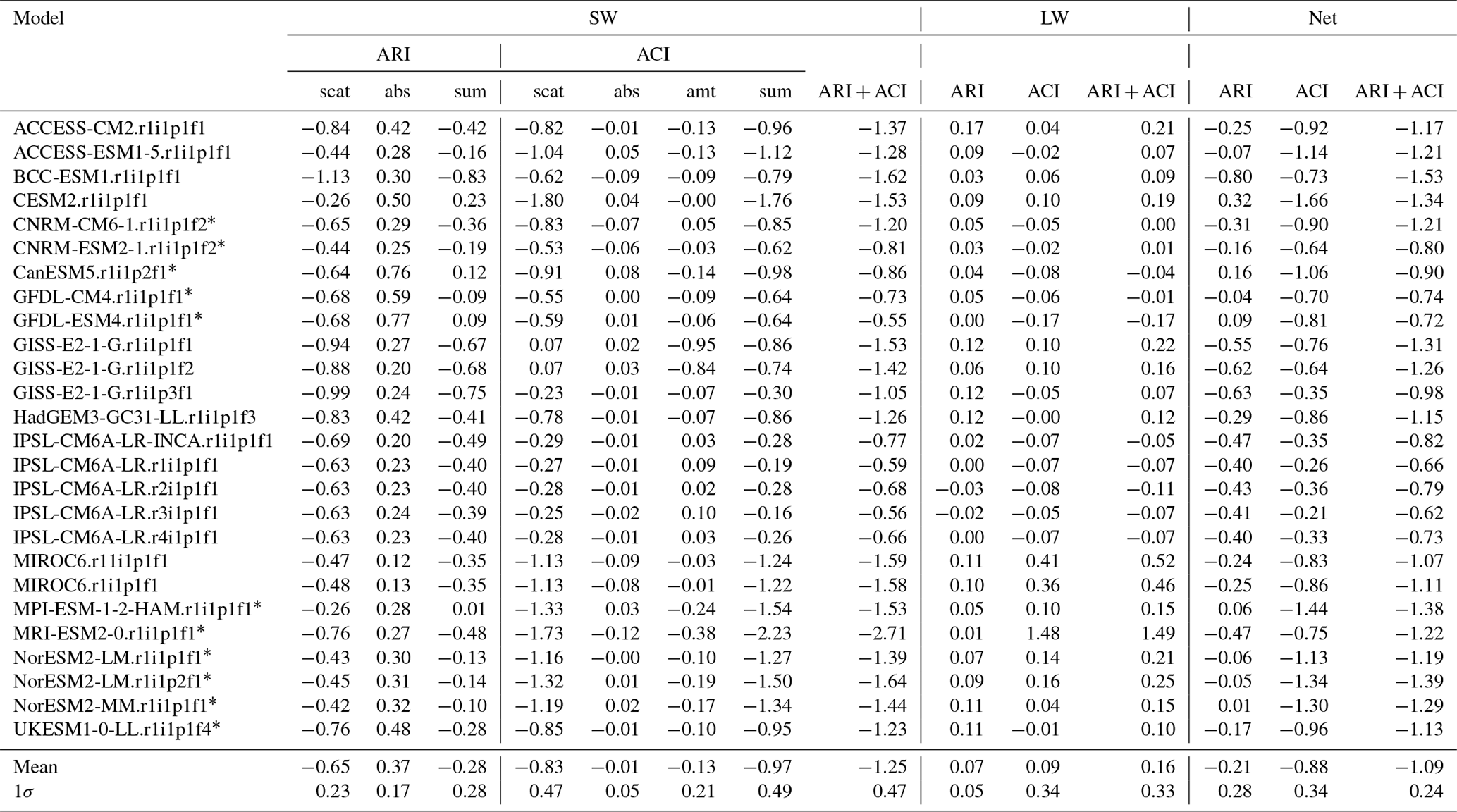
Every CMIP6 model agrees on a negative ERF${}_{\mathrm{ari}}^{\mathrm{SW}}$ due to scattering and a positive ERF${}_{\mathrm{ari}}^{\mathrm{SW}}$ due to absorption, but the relative strengths vary, leading to a lack of agreement on the sign of ERF${}_{\mathrm{ari}}^{\mathrm{SW}}$. All CMIP6 models have negative ERF${}_{\mathrm{aci}}^{\mathrm{SW}}$ values. This is due to the dominance of strong negative ERF${}_{\mathrm{aci}}^{\mathrm{SW}}$ scattering components, with two exceptions: the r1i1p1f1 and r1i1p1f2 variants of the GISS-E2-1-G model have small positive ERF${}_{\mathrm{aci}}^{\mathrm{SW}}$ cloud scattering components but anomalously strong negative ERF${}_{\mathrm{aci}}^{\mathrm{SW}}$ cloud amount components. This is consistent with the fact that the “p1” physics variants of GISS-E2-1-G parameterize aerosol effects on clouds by directly relating anthropogenic aerosol mass to a change in (only) total cloud cover (Miller et al., 2021). In the “p3” physics variants, in contrast, aerosols act as cloud condensation nuclei and change (only) cloud optical depth; hence the r1i1p3f1 variant of GISS-E2-1-G has a moderate negative ERF${}_{\mathrm{aci}}^{\mathrm{SW}}$ cloud scattering component and weak ERF${}_{\mathrm{aci}}^{\mathrm{SW}}$ cloud amount component (Table 2). In all models, ERF${}_{\mathrm{ari}+\mathrm{aci}}^{\mathrm{SW}}$ is negative.

ERF${}_{\mathrm{ari}}^{\mathrm{LW}}$ is positive in nearly all CMIP6 models but is small with opposite sign relative to its SW counterpart. ERF${}_{\mathrm{aci}}^{\mathrm{LW}}$ values are generally small except for the models identified in Smith et al. (2020) as parameterizing aerosol effects on ice clouds (CESM2, MIROC6, MRI-ESM2-0, and NorESM2-LM), for which the ERF${}_{\mathrm{aci}}^{\mathrm{LW}}$ values are non-negligible and positive. Finally, the net (LW + SW) ERF_ari+aci is systematically negative across all models, primarily due to the systematically negative indirect component that is generally larger in magnitude than the direct component, which is small or also negative.

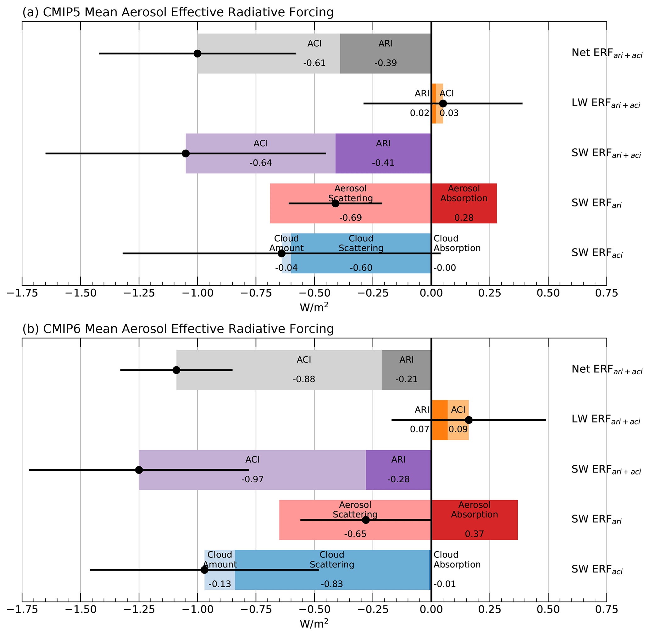
Figure 9 Global mean ERF_ari+aci values averaged across (a) CMIP5 and (b) CMIP6 models, separated into ERF_ari and ERF_aci for LW, SW, and net (LW + SW) radiation. ERF${}_{\mathrm{ari}}^{\mathrm{SW}}$ is further separated into its scattering and absorption components. ERF${}_{\mathrm{aci}}^{\mathrm{SW}}$ is further separated into its amount, scattering, and absorption components. The sum of terms in each row is indicated by the black dot, with the inter-model standard deviation of each sum indicated by the horizontal error bar.

To aid in visualizing the model results and to connect back to Fig. 10 in Zelinka et al. (2014) and Fig. 10 in Smith et al. (2020), multi-model mean ERF values are shown for both the CMIP5 and CMIP6 models in Fig. 9. We strongly caution against overinterpreting differences between the two ensembles for two reasons. First, they differ in how “present day” is defined (2000 for CMIP5 and 2014 for CMIP6). Second, the fraction of models that represent aerosol effects on cloud optical properties and/or lifetimes differs, with three CMIP5 models (FGOALS-s2, MPI-ESM-LR, and bcc-csm1-1) lacking any representation of indirect effects, some models representing only the first indirect effect, and some representing both the first and second indirect effects (Rotstayn et al., 2013; Wilcox et al., 2013). With these caveats in mind, we note that the negative net (LW + SW) ERF_aci is nearly 50 % stronger in magnitude in CMIP6, while the smaller net ERF_ari is roughly halved in CMIP6. Close compensation between these two changes means that the overall net ERF_ari+aci is only slightly larger in CMIP6. The negative ERF_aci is stronger in CMIP6 due primarily to stronger SW cooling from a greater sensitivity of cloud scattering and amount to aerosols (partly related to the fact that three models in CMIP5 do not incorporate indirect effects). The negative ERF_ari is weaker in CMIP6 due primarily to stronger SW heating from absorbing aerosols. These same conclusions hold even if we compare CMIP5 and CMIP6 averages based only on models from centers that contributed to both phases (not shown).

4 Conclusions

Accurate values of radiative forcings across a broad suite of climate models are a prerequisite for proper understanding of the drivers of inter-model differences in climate response. Model-to-model differences in aerosol radiative forcing are particularly large and come from both aerosol direct and indirect components, each of which has competing contributions from changes in scattering and absorption of SW radiation. In this study we corrected estimates of aerosol effective radiative forcing derived in Smith et al. (2020) from a collection of CMIP6 models that performed idealized aerosol perturbation experiments. We also provided values from additional CMIP6 models that became available subsequent to its publication (as well as CMIP5 models previously reported, for completeness). The errors in the previous study resulted from two larger errors that, fortuitously, largely canceled in the global mean, though for certain sub-components these errors do not cancel and are non-negligible. Most notably, the direct radiative forcing from absorbing aerosols averaged across CMIP6 models is more than 40 % larger in the present study. Aerosol effective radiative forcings derived herein have negligible residuals and agree well with values derived using an independent double-radiation-call technique, both in the global mean and in geographic structure. Code to perform the accurate APRP method is provided at the link in the “Code availability” section.

Appendix A

A1 Introduction

In this appendix, we provide further explanation of the APRP technique and how it is to be used correctly. We then explain the two implementation errors in Smith et al. (2020), the first involving the calculation of albedo sensitivities and the second involving usage of incorrect SW fluxes at the top of the atmosphere.

A2 APRP

As detailed in Taylor et al. (2007), the planetary albedo (A) can be written in terms of the surface albedo (α), an atmospheric transmittance coefficient (μ), and an atmospheric scattering coefficient (γ):

$$\begin{array}{}\text{(A1)}& A=\mathit{\mu }\mathit{\gamma }+{\displaystyle \frac{\mathit{\mu }\mathit{\alpha }(\mathrm{1}-\mathit{\gamma }{)}^{\mathrm{2}}}{\mathrm{1}-\mathit{\alpha }\mathit{\gamma }}}.\end{array}$$

Surface albedo is computed as the ratio of upwelling to downwelling SW fluxes at the surface:

$$\begin{array}{}\text{(A2)}& \mathit{\alpha }={\mathrm{SW}}_{\mathrm{SFC}}^{\uparrow }/{\mathrm{SW}}_{\mathrm{SFC}}^{\downarrow }.\end{array}$$

Atmospheric transmittance is expressed as

$$\begin{array}{}\text{(A3)}& \mathit{\mu }=A+{\widehat{Q}}_{\mathrm{SFC}}^{\downarrow }(\mathrm{1}-\mathit{\alpha }),\end{array}$$

where

$$\begin{array}{}\text{(A4)}& {\widehat{Q}}_{\mathrm{SFC}}^{\downarrow }={\displaystyle \frac{{\mathrm{SW}}_{\mathrm{SFC}}^{\downarrow }}{{\mathrm{SW}}_{\mathrm{TOA}}^{\downarrow }}}\end{array}$$

is the ratio of surface to TOA incident SW flux, and the scattering coefficient is expressed as

$$\begin{array}{}\text{(A5)}& \mathit{\gamma }={\displaystyle \frac{\mathit{\mu }-{\widehat{Q}}_{\mathrm{SFC}}^{\downarrow }}{\mathit{\mu }-\mathit{\alpha }{\widehat{Q}}_{\mathrm{SFC}}^{\downarrow }}}.\end{array}$$

All of the terms given in Eqs. (A2)–(A5) can be computed for both clear-sky fluxes and for overcast-sky fluxes. This separation into clear- and overcast-sky conditions, along with some assumptions, allows for the effects of clouds to be isolated from other atmospheric constituents (primarily aerosols in the present study). Specifically, the scattering coefficient in the overcast portion of a scene can be expressed as a combination of the scattering coefficients due to non-cloud constituents and the cloud itself:

$$\begin{array}{}\text{(A6)}& (\mathrm{1}-{\mathit{\gamma }}_{\mathrm{oc}})=(\mathrm{1}-{\mathit{\gamma }}_{\mathrm{clr}})(\mathrm{1}-{\mathit{\gamma }}_{\mathrm{cld}}),\end{array}$$

where subscripts “clr” and “oc” refer to clear- and overcast-sky conditions. Similarly, the transmissivity coefficients are related as

$$\begin{array}{}\text{(A7)}& {\mathit{\mu }}_{\mathrm{oc}}={\mathit{\mu }}_{\mathrm{clr}}{\mathit{\mu }}_{\mathrm{cld}}.\end{array}$$

This allows total planetary albedo to be expressed as the sum of clear-sky albedo scaled by the clear-sky portion of the scene and overcast-sky albedo scaled by the cloudy portion of the scene:

$$\begin{array}{}\text{(A8)}& A=(\mathrm{1}-c)A_{\mathrm{clr}}+c{A}_{\mathrm{oc}},\end{array}$$

where c is the total cloud fraction. Hence, the planetary albedo is a function of seven parameters:

$$\begin{array}{}\text{(A9)}& A=A(c,{\mathit{\alpha }}_{\mathrm{clr}},{\mathit{\alpha }}_{\mathrm{oc}},{\mathit{\mu }}_{\mathrm{clr}},{\mathit{\mu }}_{\mathrm{cld}},{\mathit{\gamma }}_{\mathrm{clr}},{\mathit{\gamma }}_{\mathrm{cld}}).\end{array}$$

The derivation of these expressions (and the assumptions made in doing so) are detailed in Taylor et al. (2007) and so are not further explained here.

Having determined all of the terms upon which planetary albedo depends, we can now substitute in values of individual coefficients from the perturbed climate experiment to isolate their individual impacts on albedo. For example, to determine the impact on planetary albedo from the change in aerosol scattering, we difference the albedo computed with (only) γ_clr taken from the perturbed experiment (indicated with superscript “pert”) and the albedo computed with all fields set to their control state (no superscript):

$$\begin{array}{}\text{(A10)}& \begin{array}{rl}{\displaystyle \frac{\partial A}{\partial {\mathit{\gamma }}_{\mathrm{clr}}}}\mathrm{\Delta }{\mathit{\gamma }}_{\mathrm{clr}}& =A(c,{\mathit{\alpha }}_{\mathrm{clr}},{\mathit{\alpha }}_{\mathrm{oc}},{\mathit{\mu }}_{\mathrm{clr}},{\mathit{\mu }}_{\mathrm{cld}},{\mathit{\gamma }}_{\mathrm{clr}}^{\mathrm{pert}},{\mathit{\gamma }}_{\mathrm{cld}})\\ & -A(c,{\mathit{\alpha }}_{\mathrm{clr}},{\mathit{\alpha }}_{\mathrm{oc}},{\mathit{\mu }}_{\mathrm{clr}},{\mathit{\mu }}_{\mathrm{cld}},{\mathit{\gamma }}_{\mathrm{clr}},{\mathit{\gamma }}_{\mathrm{cld}}).\end{array}\end{array}$$

In practice, we do this calculation twice – once as a forward calculation as shown above and once as a backward calculation in which all fields are set to their perturbed value and the isolated field is set to its control state – and then these are averaged.

A3 The albedo sensitivity error in Smith et al. (2020)

Smith et al. (2020) did not use Eq. (A9) to estimate their components but rather followed a different procedure. In the example considered above, they compute the impact on planetary albedo from the change in aerosol scattering as the sum of two terms:

$$\begin{array}{}\text{(A11)}& {\displaystyle \frac{\partial A}{\partial {\mathit{\gamma }}_{\mathrm{clr}}}}\mathrm{\Delta }{\mathit{\gamma }}_{\mathrm{clr}}=(\mathrm{1}-c){\displaystyle \frac{\partial A_{\mathrm{clr}}}{\partial {\mathit{\gamma }}_{\mathrm{clr}}}}\mathrm{\Delta }{\mathit{\gamma }}_{\mathrm{clr}}+c{\displaystyle \frac{\partial A_{\mathrm{oc}}}{\partial {\mathit{\gamma }}_{\mathrm{clr}}}}\mathrm{\Delta }{\mathit{\gamma }}_{\mathrm{clr}},\end{array}$$

where the responses of A_clr and A_oc to perturbations in γ_clr are computed by substituting directly into Eq. (A1). The error arises for the latter term, which Smith et al. compute as

$$\begin{array}{}\text{(A12)}& {\displaystyle \frac{\partial A_{\mathrm{oc}}}{\partial {\mathit{\gamma }}_{\mathrm{clr}}}}\mathrm{\Delta }{\mathit{\gamma }}_{\mathrm{clr}}=A({\mathit{\alpha }}_{\mathrm{oc}},{\mathit{\mu }}_{\mathrm{oc}},{\mathit{\gamma }}_{\mathrm{clr}}^{\mathrm{pert}})-A({\mathit{\alpha }}_{\mathrm{oc}},{\mathit{\mu }}_{\mathrm{oc}},{\mathit{\gamma }}_{\mathrm{clr}}).\end{array}$$

Note that in Eq. (A12) the clear-sky scattering coefficients are erroneously used to compute overcast-sky albedo. The correct calculation is

$$\begin{array}{}\text{(A13)}& {\displaystyle \frac{\partial A_{\mathrm{oc}}}{\partial {\mathit{\gamma }}_{\mathrm{clr}}}}\mathrm{\Delta }{\mathit{\gamma }}_{\mathrm{clr}}=A({\mathit{\alpha }}_{\mathrm{oc}},{\mathit{\mu }}_{\mathrm{oc}},{\mathit{\gamma }}_{\mathrm{oc}*}^{\mathrm{pert}})-A({\mathit{\alpha }}_{\mathrm{oc}},{\mathit{\mu }}_{\mathrm{oc}},{\mathit{\gamma }}_{\mathrm{oc}}),\end{array}$$

where we have defined ${\mathit{\gamma }}_{\mathrm{oc}*}^{\mathrm{pert}}$ via Eq. (A6):

$$\begin{array}{}\text{(A14)}& (\mathrm{1}-{\mathit{\gamma }}_{\mathrm{oc}*}^{\mathrm{pert}})=(\mathrm{1}-{\mathit{\gamma }}_{\mathrm{clr}}^{\mathrm{pert}})(\mathrm{1}-{\mathit{\gamma }}_{\mathrm{cld}}).\end{array}$$

This modified overcast-sky scattering coefficient allows changes in the clear-sky scattering coefficient to independently affect the overcast-sky scattering coefficient holding the cloud scattering fixed. Hence it incorporates the impact on atmospheric scattering under overcast-sky conditions solely from changes in clear-sky (aerosol) scattering, which is the coefficient needed to correctly estimate the influence of changes in clear-sky (aerosol) scattering on overcast-sky albedo. This is already implicitly done in the correct method involving substitution into Eq. (A10). It is only when substituting coefficients directly into Eq. (A1) (as done by Smith et al., 2020) that one has to separately account for this.

Why does this error cause an overestimate of the sensitivity of TOA albedo to aerosols relative to the correct implementation of APRP? The difference between scattering coefficients in the erroneous expression (Eq. A12) is

$$\begin{array}{}\text{(A15)}& \mathrm{\Delta }{\mathit{\gamma }}_{\mathrm{smith}}=({\mathit{\gamma }}_{\mathrm{clr}}^{\mathrm{pert}}-{\mathit{\gamma }}_{\mathrm{clr}}).\end{array}$$

In contrast, after some algebra one can show that the difference between scattering coefficients in the corrected expression (Eq. A13) is

$$\begin{array}{}\text{(A16)}& \mathrm{\Delta }{\mathit{\gamma }}_{\mathrm{true}}={\mathit{\gamma }}_{\mathrm{oc}*}^{\mathrm{pert}}-{\mathit{\gamma }}_{\mathrm{oc}}=(\mathrm{1}-{\mathit{\gamma }}_{\mathrm{cld}})({\mathit{\gamma }}_{\mathrm{clr}}^{\mathrm{pert}}-{\mathit{\gamma }}_{\mathrm{clr}}),\end{array}$$

which is equal to Δγ_smith scaled by 1−γ_cld. This scaling factor, which is less than 1, represents the attenuation of aerosol effects by the presence of clouds: the larger the cloud scattering coefficient, the greater the attenuation and hence the weaker the aerosol influence on TOA albedo. Therefore the correct formulation of APRP, which accurately accounts for this attenuation, has a weaker sensitivity of TOA albedo to changes in clear-sky (aerosol) scattering. In other words, Smith's scattering coefficient changes are overestimated by the factor

$$\begin{array}{}\text{(A17)}& {\displaystyle \frac{\mathrm{\Delta }{\mathit{\gamma }}_{\mathrm{smith}}}{\mathrm{\Delta }{\mathit{\gamma }}_{\mathrm{true}}}}={\displaystyle \frac{\mathrm{1}}{\mathrm{1}-{\mathit{\gamma }}_{\mathrm{cld}}}}.\end{array}$$

We note that similar coding errors are present in Smith et al.'s calculation of the sensitivity of overcast-sky albedo to aerosol absorption, cloud scattering, and cloud absorption. We find that the errors in the sensitivity of overcast-sky albedo to aerosol and cloud absorption are small in practice because cloud absorption of SW radiation is small. We do not detail these here for the sake of brevity.

A4 The insolation error in Smith et al. (2020)

All of the aforementioned APRP calculations yield sensitivities of planetary albedo (A) to perturbations in the seven parameters noted in Eq. (A9). These need to be multiplied by the insolation at the TOA in order to determine the impact on the TOA SW energy budget. The net absorbed SW radiation at the TOA is expressed as

$$\begin{array}{}\text{(A18)}& {\mathrm{SW}}_{\mathrm{abs}}=S(\mathrm{1}-A),\end{array}$$

where S is the SW flux at the top of the atmosphere and A is the planetary albedo. Its sensitivity to A is therefore

$$\begin{array}{}\text{(A19)}& {\displaystyle \frac{\partial {\mathrm{SW}}_{\mathrm{abs}}}{\partial A}}=-S.\end{array}$$

In Smith et al.'s formulation, S is

$$\begin{array}{}\text{(A20)}& S_{\mathrm{smith}}=({\mathrm{SW}}_{\mathrm{TOA}}^{\downarrow }-{\mathrm{SW}}_{\mathrm{TOA}}^{\uparrow }),\end{array}$$

whereas it should be

$$\begin{array}{}\text{(A21)}& S_{\mathrm{true}}={\mathrm{SW}}_{\mathrm{TOA}}^{\downarrow }.\end{array}$$

By using the net (downwelling minus upwelling) SW flux, Smith et al.'s values of the TOA radiative impact are therefore underestimated by the factor

$$\begin{array}{}\text{(A22)}& S_{\mathrm{smith}}/S_{\mathrm{true}}=\mathrm{1}-{\displaystyle \frac{{\mathrm{SW}}_{\mathrm{TOA}}^{\uparrow }}{{\mathrm{SW}}_{\mathrm{TOA}}^{\downarrow }}}=\mathrm{1}-A,\end{array}$$

which is roughly 70 %.

Table A1 Climate model output used in this study. APRP requires the first eight fields. LW ERF components are estimated using the following two fields. These 10 fields are routinely diagnosed in CMIP5 and CMIP6 models. For the double-call method, we rely upon aerosol-free radiative fluxes, which are the final four fields. These are only available for a subset of CMIP6 models. Aerosol-free upwelling SW radiation fluxes at the top of the atmosphere from the NorESM2-LM and NorESM2-MM models were found to be actually the net (downwelling minus upwelling) aerosol-free SW fluxes and were corrected prior to usage.

Ghan (2013)

Table A2 Abbreviations commonly used in this study.

Appendix B

B1 Introduction

In this appendix, we describe in greater detail how the various aerosol effective radiative forcings relate to each other and to the IPCC AR6 definitions (Forster et al., 2021). Specifically, we relate the LW ERFs defined by IPCC to the ERF proxies derived using standard model output in Sect. B2. We then relate the IPCC SW and LW ERF proxies to the ERFs derived using the Ghan (2013) double-call method (Sect. B3). Finally, the ERFs derived by the Ghan (2013) double-call method are related to those derived using the Taylor et al. (2007) APRP method (Sect. B4) and to the LW ERF proxies derived using standard model output (Sect. B5).

B2 LW ERFs: proxies derived from standard model output

One can expand our expression for ${\mathrm{ERF}}_{\mathrm{ari}}^{\mathrm{P},\mathrm{LW}}$ as

$$\begin{array}{}\text{(B1)}& {\mathrm{ERF}}_{\mathrm{ari}}^{\mathrm{P},\mathrm{LW}}=\mathrm{\Delta }{R}_{\mathrm{cs}}^{\mathrm{LW}}-\mathrm{\Delta }{R}_{\mathrm{cs}}^{T_{\mathrm{0}}}={\mathrm{IRF}}_{\mathrm{ari},\mathrm{cs}}^{\mathrm{LW}}+K_{\mathrm{cs}}^T\mathrm{\Delta }T+K_{\mathrm{cs}}^{q,\mathrm{LW}}\mathrm{\Delta }q.\end{array}$$

Given the IPCC definition of direct effective radiative forcing (Eq. 2), we can express our proxy as

$$\begin{array}{}\text{(B2)}& {\mathrm{ERF}}_{\mathrm{ari}}^{\mathrm{P},\mathrm{LW}}={\mathrm{ERF}}_{\mathrm{ari}}^{\mathrm{LW}}-K^{C,\mathrm{LW}}\mathrm{\Delta }{C}_{\mathrm{semidirect}}-M_{\mathrm{cld}}^{\mathrm{LW}},\end{array}$$

where

$$\begin{array}{}\text{(B3)}& \begin{array}{rl}{M}_{\mathrm{cld}}^{\mathrm{LW}}& =({\mathrm{IRF}}_{\mathrm{ari}}^{\mathrm{LW}}-{\mathrm{IRF}}_{\mathrm{ari},\mathrm{cs}}^{\mathrm{LW}})+(K^T-K_{\mathrm{cs}}^T)\mathrm{\Delta }T\\ & +(K^{q,\mathrm{LW}}-K_{\mathrm{cs}}^{q,\mathrm{LW}})\mathrm{\Delta }q.\end{array}\end{array}$$

Therefore in the LW, our proxy for the direct effect equals IPCC's direct effect minus the semidirect effect minus masking terms that quantify how much the radiative impact of rapid changes in temperature, humidity, and aerosols is attenuated by the presence of clouds.

Turning now to the LW indirect effect, we note that the change in all-sky TOA net LW radiation is given by

$$\begin{array}{}\text{(B4)}& \mathrm{\Delta }{R}^{\mathrm{LW}}={\mathrm{IRF}}_{\mathrm{ari}}^{\mathrm{LW}}+K^T\mathrm{\Delta }T+K^{q,\mathrm{LW}}\mathrm{\Delta }q+K^{C,\mathrm{LW}}\mathrm{\Delta }C.\end{array}$$

Therefore,

$$\begin{array}{}\text{(B5)}& {\mathrm{ERF}}_{\mathrm{aci}}^{\mathrm{P},\mathrm{LW}}=K^{C,\mathrm{LW}}\mathrm{\Delta }C+M_{\mathrm{cld}}^{\mathrm{LW}},\end{array}$$

where $M_{\mathrm{cld}}^{\mathrm{LW}}$ is defined above. Putting this in terms of IPCC nomenclature:

$$\begin{array}{}\text{(B6)}& {\mathrm{ERF}}_{\mathrm{aci}}^{\mathrm{P},\mathrm{LW}}={\mathrm{ERF}}_{\mathrm{aci}}^{\mathrm{LW}}+K^{C,\mathrm{LW}}\mathrm{\Delta }{C}_{\mathrm{semidirect}}+M_{\mathrm{cld}}^{\mathrm{LW}}.\end{array}$$

Therefore in the LW, our proxy for the indirect effect equals IPCC's indirect effect plus the semidirect effect plus masking terms that quantify how much the radiative impact of changes in temperature, humidity, and aerosols is attenuated by the presence of clouds. The sum of the direct and indirect LW effects are the same, independent of how the individual components are defined. Thus, from Eqs. (B2) and (B6),

$$\begin{array}{}\text{(B7)}& {\mathrm{ERF}}_{\mathrm{ari}}^{\mathrm{P},\mathrm{LW}}+{\mathrm{ERF}}_{\mathrm{aci}}^{\mathrm{P},\mathrm{LW}}={\mathrm{ERF}}_{\mathrm{ari}}^{\mathrm{LW}}+{\mathrm{ERF}}_{\mathrm{aci}}^{\mathrm{LW}}.\end{array}$$

B3 Double-radiation-call method

B3.1 Ghan's direct effect

Expanding Eq. (14), one can express the change in TOA net radiation as

$$\begin{array}{}\text{(B8)}& \mathrm{\Delta }R={\mathrm{ERF}}_{\mathrm{ari}}^{\mathrm{G}}+K_{\mathrm{af}}^T\mathrm{\Delta }T+K_{\mathrm{af}}^q\mathrm{\Delta }q+K_{\mathrm{af}}^{\mathit{\alpha }}\mathrm{\Delta }\mathit{\alpha }+K_{\mathrm{af}}^C\mathrm{\Delta }C\end{array}$$

or, equivalently,

$$\begin{array}{}\text{(B9)}& \mathrm{\Delta }R={\mathrm{IRF}}_{\mathrm{ari}}+K^T\mathrm{\Delta }T+K^q\mathrm{\Delta }q+K^{\mathit{\alpha }}\mathrm{\Delta }\mathit{\alpha }+K^C\mathrm{\Delta }C.\end{array}$$

Combining the previous two equations yields an expression for Ghan's ${\mathrm{ERF}}_{\mathrm{ari}}^{\mathrm{G}}$ in terms of the true instantaneous aerosol direct forcing:

$$\begin{array}{}\text{(B10)}& {\mathrm{ERF}}_{\mathrm{ari}}^{\mathrm{G}}={\mathrm{IRF}}_{\mathrm{ari}}-M_{\mathrm{aer}},\end{array}$$

where the aerosol masking is given by

$$\begin{array}{}\text{(B11)}& \begin{array}{rl}{M}_{\mathrm{aer}}& =(K_{\mathrm{af}}^T-K^T)\mathrm{\Delta }T+(K_{\mathrm{af}}^q-K^q)\mathrm{\Delta }q\\ & +(K_{\mathrm{af}}^{\mathit{\alpha }}-K^{\mathit{\alpha }})\mathrm{\Delta }\mathit{\alpha }+(K_{\mathrm{af}}^C-K^C)\mathrm{\Delta }C.\end{array}\end{array}$$

Therefore Ghan's direct aerosol radiative forcing equals IPCC's instantaneous direct forcing minus masking terms that quantify how much the radiative impact of changes in temperature, humidity, surface albedo, and clouds is attenuated by the presence of aerosols.

B3.2 Ghan's indirect effect

Turning now to the indirect effect, let us write the change in TOA energy budget change as

$$\begin{array}{}\text{(B12)}& \begin{array}{rl}\mathrm{\Delta }R& ={\mathrm{ERF}}_{\mathrm{ari}}^{\mathrm{G}}+{\mathrm{ERF}}_{\mathrm{aci}}^{\mathrm{G}}+K_{\mathrm{af},\mathrm{cs}}^T\mathrm{\Delta }T+K_{\mathrm{af},\mathrm{cs}}^q\mathrm{\Delta }q\\ & +K_{\mathrm{af},\mathrm{cs}}^{\mathit{\alpha }}\mathrm{\Delta }\mathit{\alpha }.\end{array}\end{array}$$

Defining

$$\begin{array}{}\text{(B13)}& \begin{array}{rl}{M}_{\mathrm{aer},\mathrm{cld}}& =(K_{\mathrm{af},\mathrm{cs}}^T-K^T)\mathrm{\Delta }T+(K_{\mathrm{af},\mathrm{cs}}^q-K^q)\mathrm{\Delta }q\\ & +(K_{\mathrm{af},\mathrm{cs}}^{\mathit{\alpha }}-K^{\mathit{\alpha }})\mathrm{\Delta }\mathit{\alpha },\end{array}\end{array}$$

which measures how much the radiative impact of changes in temperature, humidity, and surface albedo are masked by clouds and aerosols, and combining Eqs. (B9) and (B11) yields an expression for the total cloud-induced radiation anomalies in terms of ${\mathrm{ERF}}_{\mathrm{aci}}^{\mathrm{G}}$:

$$\begin{array}{}\text{(B14)}& K^C\mathrm{\Delta }C={\mathrm{ERF}}_{\mathrm{ari}}^{\mathrm{G}}+{\mathrm{ERF}}_{\mathrm{aci}}^{\mathrm{G}}-{\mathrm{IRF}}_{\mathrm{ari}}+M_{\mathrm{aer},\mathrm{cld}}.\end{array}$$

Given Eq. (B10), we can therefore write

$$\begin{array}{}\text{(B15)}& K^C\mathrm{\Delta }C={\mathrm{ERF}}_{\mathrm{aci}}^{\mathrm{G}}-M_{\mathrm{aer}}+M_{\mathrm{aer},\mathrm{cld}}\end{array}$$

or, equivalently,

$$\begin{array}{}\text{(B16)}& \begin{array}{rl}{K}^C\mathrm{\Delta }C& ={\mathrm{ERF}}_{\mathrm{aci}}^{\mathrm{G}}+(K_{\mathrm{af},\mathrm{cs}}^T-K_{\mathrm{af}}^T)\mathrm{\Delta }T+(K_{\mathrm{af},\mathrm{cs}}^q-K_{\mathrm{af}}^q)\mathrm{\Delta }q\\ & +(K_{\mathrm{af},\mathrm{cs}}^{\mathit{\alpha }}-K_{\mathrm{af}}^{\mathit{\alpha }})\mathrm{\Delta }\mathit{\alpha }+(K^C-K_{\mathrm{af}}^C)\mathrm{\Delta }C.\end{array}\end{array}$$

We can now express Ghan's ${\mathrm{ERF}}_{\mathrm{aci}}^{\mathrm{G}}$ in terms of IPCC's aerosol indirect forcing:

$$\begin{array}{}\text{(B17)}& {\mathrm{ERF}}_{\mathrm{aci}}^{\mathrm{G}}={\mathrm{ERF}}_{\mathrm{aci}}+M_{\mathrm{aer}}-M_{\mathrm{aer},\mathrm{cld}}+K^C\mathrm{\Delta }{C}_{\mathrm{semidirect}}.\end{array}$$

Therefore Ghan's indirect effect equals IPCC's indirect effect plus masking terms that quantify how much the radiative impact of changes in temperature, humidity, and surface albedo is attenuated by the presence of clouds under aerosol-free conditions and how much the radiative impact of changes in clouds is attenuated by the presence of aerosols plus the semidirect effect.

B3.3 Ghan's other forcing term

Finally, let us separate the third forcing term defined by Ghan (2013) into its LW and SW components:

$$\begin{array}{}\text{(B18)}& {\mathrm{ERF}}_{\mathrm{other}}^{\mathrm{G},\mathrm{LW}}=K_{\mathrm{af},\mathrm{cs}}^T\mathrm{\Delta }T+K_{\mathrm{af},\mathrm{cs}}^{q,\mathrm{LW}}\mathrm{\Delta }q\end{array}$$

and

$$\begin{array}{}\text{(B19)}& {\mathrm{ERF}}_{\mathrm{other}}^{\mathrm{G},\mathrm{SW}}=K_{\mathrm{af},\mathrm{cs}}^{q,\mathrm{SW}}\mathrm{\Delta }q+K_{\mathrm{af},\mathrm{cs}}^{\mathit{\alpha }}\mathrm{\Delta }\mathit{\alpha }.\end{array}$$

We can expand ${\mathrm{ERF}}_{\mathrm{other}}^{\mathrm{G},\mathrm{SW}}$ as

$$\begin{array}{}\text{(B20)}& {\mathrm{ERF}}_{\mathrm{other}}^{\mathrm{G},\mathrm{SW}}=\mathrm{\Delta }{R}_{\mathrm{alb}}^{\mathrm{SW}}+K_{\mathrm{af},\mathrm{cs}}^{q,\mathrm{SW}}\mathrm{\Delta }q+(K_{\mathrm{af},\mathrm{cs}}^{\mathit{\alpha }}-K^{\mathit{\alpha }})\mathrm{\Delta }\mathit{\alpha }.\end{array}$$

Therefore ${\mathrm{ERF}}_{\mathrm{other}}^{\mathrm{G},\mathrm{SW}}$ – which Ghan (2013) refers to as the surface albedo forcing – equals $\mathrm{\Delta }{R}_{\mathrm{alb}}^{\mathrm{SW}}$ plus the aerosol-free clear-sky radiative contributions from changes in humidity plus a masking term that quantifies how much the radiative impact of changes in surface albedo is attenuated by the presence of both clouds and aerosols.

B4 Relating SW ERF terms: Ghan (2013) vs. APRP

Combining Eqs. (7) and (B10) yields the relationship between Ghan- and APRP-derived SW direct radiative forcing:

$$\begin{array}{}\text{(B21)}& {\mathrm{ERF}}_{\mathrm{ari}}^{\mathrm{A},\mathrm{SW}}={\mathrm{ERF}}_{\mathrm{ari}}^{\mathrm{G},\mathrm{SW}}+M_{\mathrm{aer}}^{\mathrm{SW}}+K^{q,\mathrm{SW}}\mathrm{\Delta }q.\end{array}$$

Because K^C,SWΔC is equivalent to ${\mathrm{ERF}}_{\mathrm{aci}}^{\mathrm{A},\mathrm{SW}}$ (cf. Eqs. 5 and 7), a simple substitution into Eq. (B15) (applied to the shortwave) yields the relationship between the APRP and Ghan (2013) representations of the SW indirect effect:

$$\begin{array}{}\text{(B22)}& {\mathrm{ERF}}_{\mathrm{aci}}^{\mathrm{A},\mathrm{SW}}={\mathrm{ERF}}_{\mathrm{aci}}^{\mathrm{G},\mathrm{SW}}-M_{\mathrm{aer}}^{\mathrm{SW}}+M_{\mathrm{aer},\mathrm{cld}}^{\mathrm{SW}}.\end{array}$$

Similarly the relation between APRP's surface albedo component and Ghan's equivalent (${\mathrm{ERF}}_{\mathrm{other}}^{\mathrm{G},\mathrm{SW}}$) is already expressed in Eq. (B20):

$$\begin{array}{}\text{(B23)}& \mathrm{\Delta }{R}_{\mathrm{alb}}^{\mathrm{A},\mathrm{SW}}={\mathrm{ERF}}_{\mathrm{other}}^{\mathrm{G},\mathrm{SW}}-K_{\mathrm{af},\mathrm{cs}}^{q,\mathrm{SW}}\mathrm{\Delta }q-(K_{\mathrm{af},\mathrm{cs}}^{\mathit{\alpha }}-K^{\mathit{\alpha }})\mathrm{\Delta }\mathit{\alpha }.\end{array}$$

B5 Relating LW ERF terms: Ghan (2013) vs. proxies

Subtracting Eqs. (14) and (16) from Eq. (11) and rearranging terms, we can write

$$\begin{array}{}\text{(B24)}& {\mathrm{ERF}}_{\mathrm{ari}}^{\mathrm{P},\mathrm{LW}}={\mathrm{ERF}}_{\mathrm{ari}}^{\mathrm{G},\mathrm{LW}}+{\mathrm{ERF}}_{\mathrm{other}}^{\mathrm{G},\mathrm{LW}}-\mathrm{\Delta }{R}_{\mathrm{cs}}^{T_{\mathrm{0}}}+\mathit{ϵ},\end{array}$$

where

$$\begin{array}{}\text{(B25)}& \begin{array}{rl}\mathit{ϵ}& =(\mathrm{\Delta }{R}_{\mathrm{cs}}^{\mathrm{LW}}-\mathrm{\Delta }{R}^{\mathrm{LW}})-(\mathrm{\Delta }{R}_{\mathrm{af},\mathrm{cs}}^{\mathrm{LW}}-\mathrm{\Delta }{R}_{\mathrm{af}}^{\mathrm{LW}})\\ & =\mathrm{\Delta }{\mathrm{CRE}}^{\mathrm{LW}}-\mathrm{\Delta }{\mathrm{CRE}}_{\mathrm{af}}^{\mathrm{LW}}\end{array}\end{array}$$

is very small because the change in LW cloud radiative effect is roughly the same under aerosol-free and aerosol-present conditions. This means that our proxy for longwave direct effect equals the sum of Ghan's direct effect and “other” term plus adjustments that account for the radiative impact of surface temperature change and differences in the CRE response under aerosol-free and aerosol-present conditions. Combining Eqs. (B6) and (B17) yields the relationship between the Ghan- and proxy-derived estimates of the LW indirect effect:

$$\begin{array}{}\text{(B26)}& {\mathrm{ERF}}_{\mathrm{aci}}^{\mathrm{P},\mathrm{LW}}={\mathrm{ERF}}_{\mathrm{aci}}^{\mathrm{G},\mathrm{LW}}-M_{\mathrm{aer}}^{\mathrm{LW}}+M_{\mathrm{aer},\mathrm{cld}}^{\mathrm{LW}}+M_{\mathrm{cld}}^{\mathrm{LW}}.\end{array}$$

In the LW, M_aer is zero, so

$$\begin{array}{}\text{(B27)}& {\mathrm{ERF}}_{\mathrm{aci}}^{\mathrm{P},\mathrm{LW}}={\mathrm{ERF}}_{\mathrm{aci}}^{\mathrm{G},\mathrm{LW}}+M_{\mathrm{aer},\mathrm{cld}}^{\mathrm{LW}}+M_{\mathrm{cld}}^{\mathrm{LW}}.\end{array}$$

This means that our proxy for longwave indirect effect equals Ghan's indirect effect plus masking terms quantifying how strongly clouds attenuate the LW impact of changes in temperature, humidity, and aerosols and how strongly clouds and aerosols together attenuate the LW impact of changes in temperature and humidity.