the Creative Commons Attribution 4.0 License.
the Creative Commons Attribution 4.0 License.
 | 23 Jan 2023
Reconstructing volcanic radiative forcing since 1990, using a comprehensive emission inventory and spatially resolved sulfur injections from satellite data in a chemistry-climate model
Jennifer Schallock
Christoph Brühl
Christine Bingen
Michael Höpfner
Landon Rieger
Jos Lelieveld
This paper presents model simulations of stratospheric aerosols with a focus on explosive volcanic eruptions. Using various (occultation and limb-based) satellite instruments, providing vertical profiles of sulfur dioxide (SO2) and aerosol extinction, we characterized the chemical and radiative influence of volcanic aerosols for the period between 1990 and 2019.
We established an improved and extended volcanic SO2 emission inventory that includes more than 500 explosive volcanic eruptions reaching the upper troposphere and the stratosphere. Each perturbation identified was derived from the satellite data and incorporated as a three-dimensional SO2 plume into a chemistry-climate model without the need for additional assumptions about altitude distribution and eruption duration as needed for a “point source” approach.
The simultaneous measurements of SO2 and aerosol extinction by up to four satellite instruments enabled a reliable conversion of extinction measurements into injected SO2. In the chemistry-climate model, the SO2 from each individual plume was converted into aerosol particles and their optical properties were determined. Furthermore, the aerosol optical depth (AOD) and the instantaneous radiative forcing on climate were calculated online. Combined with model improvements, the results of the simulations are consistent with the observations of the various satellites.
Slight deviations between the observations and model simulations were found for the large volcanic eruption of Pinatubo in 1991 and cases where simultaneous satellite observations were not unique or too sparse. Weak- and medium-strength volcanic eruptions captured in satellite data and the Smithsonian database typically inject about 10 to 50 kt SO2 directly into the upper troposphere/lower stratosphere (UTLS) region or the sulfur species are transported via convection and advection. Our results confirm that these relatively minor eruptions, which occur quite frequently, can nevertheless contribute to the stratospheric aerosol layer and are relevant for the Earth's radiation budget. These minor eruptions cause a total global instantaneous radiative forcing of the order of −0.1 W m−2 at the top of the atmosphere (TOA) compared to a background stratospheric aerosol forcing of about −0.04 W m−2. Medium-strength eruptions injecting about 400 kt SO2 into the stratosphere or accumulation of consecutive smaller eruptions can lead to a total instantaneous forcing of about −0.3 W m−2. We show that it is critical to include the contribution of the extratropical lowermost stratospheric aerosol in the forcing calculations.
- Article
(16554 KB) - Full-text XML
-
Supplement
(746 KB) - BibTeX
- EndNote


Next to recent historical events in which large fires have become a major source of aerosols up to the tropopause and above (Kloss et al., 2019), stratospheric aerosol particles are mostly of volcanic origin and consist of an internal liquid mixture of sulfuric acid (H2SO4) and water (H2O) (Vernier et al., 2011). The typical median diameter of these aerosol particles ranges between 200 nm for the background aerosol and 600 nm for Pinatubo conditions (Wilson et al., 2008). In this study, we incorporated stratospheric aerosol, the sulfur chemistry and the radiative transfer into a comprehensive chemistry-climate model (CCM), which we have used to gain a better understanding of the interaction of aerosols with the global climate system, including chemical effects. Particular emphasis is being placed on adequately modelling and understanding the impact of volcanic eruptions and other aerosol sources on the evolution of the stratospheric aerosol burden.
Sulfate and ashes from explosive volcanic eruptions can account for the majority of the aerosol burden in the stratosphere during volcanically active periods and cause strong temporal and spatial variations in the concentration and the size distribution of the particles (Vernier et al., 2011). These changes influence in turn the radiative forcing at the top of the atmosphere (or at tropopause altitude) for several years after strong eruptions (Timmreck, 2012) and can even have a more prolonged impact on the global climate (McGregor et al., 2015). After such a volcanic eruption, the enhanced radiative heating in the stratosphere exerts an effect on dynamics, influences the global spread of the volcanic cloud and leads to an upward transport of the aerosol itself as well as other chemical tracers, including ozone (Timmreck et al., 1999). The aerosol radiative heating resulting from large volcanic eruptions like Pinatubo triggers enhanced tropical upwelling, which causes a lofting of the injected SO2 (sulfur dioxide) and the aerosol as well as other compounds. The radiative feedback on dynamics is required to model aerosol extinction in the upper part of the volcanic aerosol plume that corresponds to observations (e.g. Aquila et al., 2012; Toohey et al., 2011).
Due to the large variability in volcanic emissions, it is challenging to estimate future trends for stratospheric optical depth and forcing (Swindles et al., 2018; Fasullo et al., 2017; Aubry et al., 2021). Therefore, the influence of volcanic eruptions is not included in predictive simulations for future climate scenarios in the IPCC report of 2013 (IPCC, 2013).
Previous studies show that model simulations often cannot fully reproduce the aerosol optical depth (AOD) of satellite observations or the derived global forcing of the stratospheric aerosol layer (Solomon et al., 2011), because the number of volcanic eruptions reaching the stratosphere and treated explicitly appears to be underestimated in most analyses (Mills et al., 2016; Brühl et al., 2015; Schmidt et al., 2018; Andersson et al., 2015). Conversely, the intensity of single eruptions can sometimes be overestimated because of incorrect vertical distribution of the injection patterns in the models (e.g. Kasatochi compared to Glantz et al., 2014). In previous studies smaller volcanic eruptions have often been included in the background atmosphere, even though they can be responsible for a radiative forcing that is twice as strong as the non-volcanic background conditions in volcanically quiescent periods such as from 1999 to 2002 (IPCC, 2013; Solomon et al., 2011; Vernier et al., 2011). Friberg et al. (2018) included the entire time series of CALIOP (Cloud-Aerosol Lidar with Orthogonal Polarization) data from 2006 to 2015 and derived stratospheric AOD using reanalysis data for the tropopause but only mention medium-sized eruptions explicitly. Radiative forcing is estimated in this case by multiplying AOD by a factor of −25 (Hansen et al., 2005) rather than using a radiative transfer model, an approximation valid in the absence of major forest fires (see e.g. Sellitto et al., 2022).
The model simulations in this study are compared to GloSSAC V2 (Thomason et al., 2018; Kovilakam et al., 2020), a time-dependent multi-satellite zonal average aerosol climatology which provides extinction data (Fig. C1 in Appendix C1). In our approach we consider as much as possible small eruptions reaching the stratosphere explicitly. For this purpose we calculate SO2 injections into the stratosphere based on the Smithsonian volcano database and the most recent releases of satellite datasets, in particular those gathered using limb sounding instruments to derive information on the vertical distribution.
For the ENVISAT (European Environmental Satellite) period 2002–2012 a first version of a new volcanic SO2 inventory with improved temporal and spatial resolution was developed within the framework of ISAMIP (https://isamip.eu, last access: 10 January 2023) (Timmreck et al., 2018; Brühl et al., 2018). The corresponding database (https://doi.org/10.1594/WDCC/SSIRC_1; Brühl, 2018) contains three-dimensional SO2 perturbations derived from satellite data as well as integrated injected SO2 masses. In this work the database is expanded to the period 1990–2019 and is considerably improved for the period 1998–2001. The simultaneous measurements from up to four instruments from 2002 to 2012 enabled us to develop a novel procedure for conversion of aerosol extinction to SO2 needed for the period before and after ENVISAT.
Our method circumvents problems and uncertainties related to the classical point source approach like dependence on the model grid box size and exact location as well as the assumed vertical distribution, the assumed time interval during which the mass is injected, and effects of microphysical and chemical interactions of SO2 and sulfate with injected volcanic ash and water in the early phase (Zhu et al., 2020). Since simulations of point source emissions are very sensitive to the emission conditions, in some cases it may be more appropriate to implement the main plume of volcanic emissions in the model not directly at the volcano location but instead apply other coordinates according to satellite observations. A case study for point source emissions is shown in Appendix C3.
Non-eruptive permanently degassing volcanoes represent another natural source of aerosols, which are treated separately from active explosive volcanic eruptions. For the stratosphere these contribute in most cases only to the background since most but not all of the released SO2 is removed by oxidation and rainout in the troposphere and only a small fraction can reach the stratosphere by convection and large-scale transport. This holds also for the medium-sized eruption of Eyjafjallajökull in 2010 from which almost no SO2 reached the stratosphere, as shown by MIPAS observations. Stratospheric H2SO4 is also produced from non-volcanic sulfur precursor gases, like carbonyl sulfide (OCS) (Crutzen, 1976), dimethyl sulfide (DMS) (Kettle and Andreae, 2000), and tropospheric SO2 from pollution, which constitute a source of background concentration of stratospheric aerosol.
This paper is structured as follows: Sect. 2 presents satellite data used for entering the volcanic perturbations of aerosols and SO2 into the model and for model evaluation. In Sect. 3, the set-up used for the climate model simulations is described. Section 4 contains a volcanic sulfur emission inventory with all relevant explosive volcanic eruptions detected between 1990 and 2019, which are included in the model simulations in Sect. 5. The influence of these volcanic eruptions on the stratosphere and climate is analysed in Sect. 6. At the end of Sect. 6 as well as in the final discussion (Sect. 7), the results are discussed in a wider context.
To generate the input data from volcanic eruptions for our simulations, we analysed satellite datasets from two instruments on the European Environmental Satellite (ENVISAT) that was launched on 1 March 2002 and lost signal on 8 April 2012, namely MIPAS (SO2 data) and Global Ozone Monitoring by Occultation of Stars (GOMOS – aerosol extinction data). Furthermore, the OSIRIS instrument on board the Odin satellite was used to provide additional aerosol extinction data for the period up to 2019. For the period before 2002, we used the SAGE II instrument for aerosol extinction data. The data processing is described in Sect. 4. Some examples of eruptions where simultaneous observations from all these instruments or at least three were available for cross-validation are presented in Appendix B.
2.1 Michelson Interferometer for Passive Atmospheric Sounding (MIPAS)
MIPAS was a mid-infrared emission spectrometer on board the ENVISAT satellite. MIPAS scanned the limb, thereby analysing the infrared radiation emitted by the Earth's atmosphere at different tangent altitudes (Fischer et al., 2008).
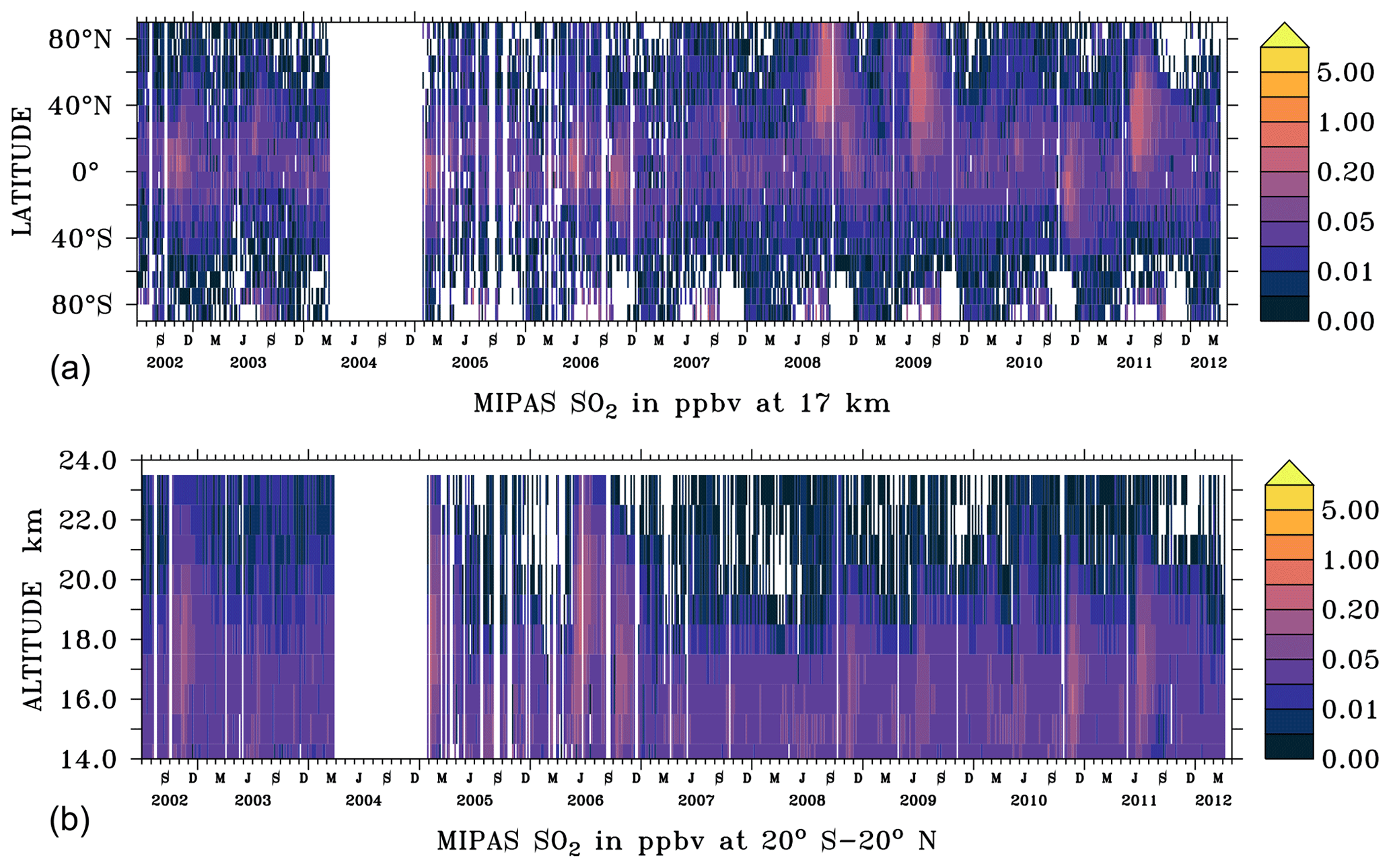
Figure 1The volume mixing ratios of SO2 in ppbv as derived from the MIPAS instrument (Höpfner et al., 2015). The dataset spans the period 1 July 2002–8 April 2012 (5 d averages). Horizontal distribution at 17 km altitude (a) and vertical distribution for tropical regions 20∘ S–20∘ N (b). White: no data.
The atmospheric spectra ranging from 4.15 to 14.6 µm are inverted to provide vertical profiles of temperature and volume mixing ratios of more than 25 different trace species, like the sulfate aerosol precursor gases SO2 and OCS (Glatthor et al., 2015, 2017; Höpfner et al., 2013, 2015), as well as H2O, ozone (O3), methane (CH4), nitrous oxide (N2O), nitrogen dioxide (NO2), and nitric acid (HNO3).
Vertical SO2 profiles (Fig. 1) from the MIPAS SO2 single profile retrieval (Höpfner et al., 2015) were used to identify plumes of volcanic eruptions. We utilized a gridded dataset from these retrievals with a three-dimensional sampling of 60∘ longitude, 10∘ latitude, and 1 km altitude with a vertical coverage of 10 to 23 km and a temporal averaging of 5 d. The lower-altitude limit varies with the tops of clouds in the troposphere, especially in tropical regions.
The typical random uncertainty for a single measurement of a volume mixing ratio profile is estimated to be 70–100 pptv. For the gridded dataset used here, systematic uncertainties are more important. These were estimated to be 10–75 pptv (10 %–180 %) under background conditions of the upper troposphere/lower stratosphere (UTLS) and 10–110 pptv (10 %–75 %) under volcanic influence (Höpfner et al., 2015).
2.2 GOMOS
The GOMOS instrument on ENVISAT operates based on the principle of stellar occultation. GOMOS provides data on stratospheric aerosol extinction as well as O3, NO2, nitrogen trioxide (NO3) and air density (Kyrölä et al., 2010). The principle of stellar occultation is described in detail in Bertaux et al. (2010). In short, this self-calibrating sounding method scans the atmosphere by pointing to a star during its set or rise. The measured spectra vary with the tangent altitude due to the absorption and scattering of light by the different atmospheric species along the line of sight.
In a first step, the GOMOS inversion algorithm determines the slant column density of gaseous species and the slant aerosol optical depth along the optical path (Vanhellemont et al., 2004). This process makes use of reference absorption spectra of the main absorbing species, such as the ones provided by the MPI-Mainz UV/VIS Spectral Atlas of Gaseous Molecules of Atmospheric Interest (https://www.uv-vis-spectral-atlas-mainz.org/uvvis/, last access: 10 January 2023) and extinction cross-section values representative for aerosols. Also, it requires the removal of the contribution of Rayleigh scattering by neutral air, which has to be carefully estimated, because satellite measurements cannot discriminate the contributions of neutral air density and very small particles compared to the wavelength (e.g. new particles arising from the conversion of SO2 to fresh aerosol particles), respectively. In a second step, vertical density profiles of the target gas species and vertical profiles of the aerosol extinction coefficient are obtained from the slant quantities (Bertaux et al., 2010).
GOMOS uses four spectrometers providing measurements at wavelengths from the UV-visible range to the near-IR range in four spectral regions: 248–371, 387–693, 750–776, and 915–956 nm (Robert et al., 2016). As the original inversion algorithm (the operational algorithm IPF – Instrument Processor Facility) was poorly effective for the retrieval of the aerosol extinction coefficient and only one extinction channel was obtained at the reference wavelength of 550 nm (Vanhellemont et al., 2010), a new retrieval algorithm called AerGOM was designed (Vanhellemont et al., 2016; Robert et al., 2016) in order to improve the spectral inversion. The main changes brought to AerGOM concern a change in the retrieval strategy where all atmospheric contributions are retrieved all together instead of one by one, a revision of the parametrization of the aerosol spectral dependence, and a more accurate estimate of the scattering cross section by air. Also, the cross-section spectra for the gaseous species were revised using up-to-date reference spectra (Bingen et al., 2019). AerGOM provides the spectral dependence of the aerosol extinction coefficient between about 350 and 750 nm.
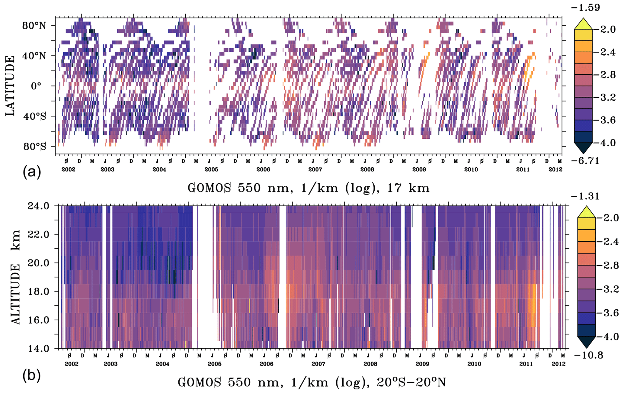
Figure 2The decadal logarithm (log) of the aerosol extinction coefficient (km−1) as derived from the GOMOS instrument data v.3.00 at a 550 nm wavelength from Bingen et al. (2017). The dataset spans the period 15 April 2002–8 April 2012 (5 d averages). Horizontal distribution at 17 km altitude (a) and vertical distribution for tropical regions 20∘ S–20∘ N (b). Maximum and minimum values appear above (yellow) and below (dark blue) the colour keys, respectively. White: no data.
The typical extinction uncertainty exhibits large variability as a function of the star parameters (from about 5 %–15 % in the most favourable cases of bright, hot stars to about 40 %–70 % in the less favourable cases of dim, cold stars) (Bingen et al., 2017). A full validation of AerGOM, version 1.0, is presented by Vanhellemont et al. (2016). The main factor influencing the uncertainty is the weakness of the star signal, which is alleviated by the high measurement rate made possible by the abundance of stars. The large variability in the magnitude and temperature of the occultated stars also significantly influences the measurement uncertainty (Robert et al., 2016).
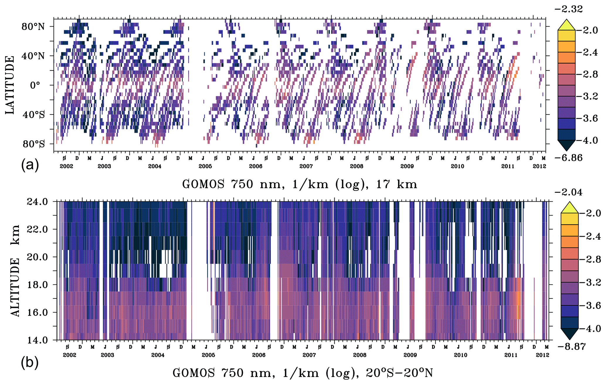
From AerGOM, climate data records were processed for use in chemistry-climate models (Bingen et al., 2017), and these are the datasets used in the present study. Figures 2 and 3 show the aerosol extinction from the GOMOS instrument at wavelengths of 550 nm (Fig. 2) and 750 nm (Fig. 3), respectively. In both cases, a gridded aerosol extinction dataset is used (CCI-GOMOS dataset in version 3.00; see Bingen et al., 2017).
The resolution of the CCI-GOMOS dataset was optimized to a grid of 5∘ latitude by 60∘ longitude and a time resolution of 5 d. This choice is made possible by the high measurement rate and is more suitable for describing the aerosol distribution than zonal monthly means, because it allows detection of the signature of aerosol patterns with a lifetime of as short as a week (e.g. medium-sized volcanic eruptions).
2.3 Optical Spectrograph and InfraRed Imaging System (OSIRIS)
The dataset from OSIRIS allowed us to extend the time series beyond April 2012, after which the signal of the ENVISAT satellite was lost. OSIRIS is a limb scatter instrument, which was launched on board the Odin satellite on 20 February 2001 and is still operating today.
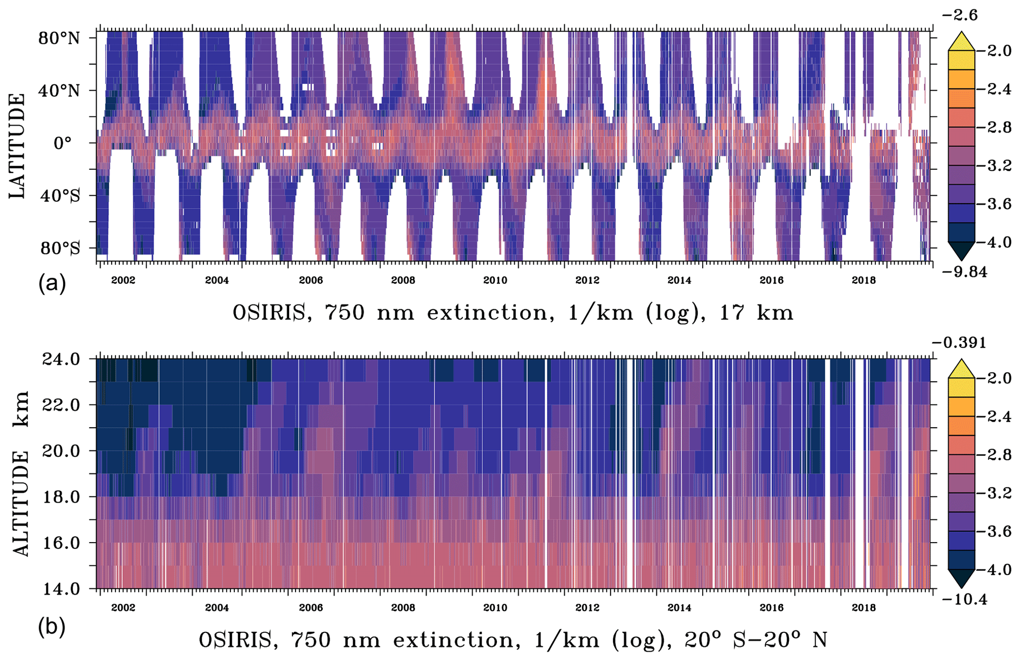
Figure 4The logarithm log (km−1) of the aerosol extinction as derived from the OSIRIS instrument at a 750 nm wavelength by Bourassa et al. (2012a) and Rieger et al. (2019). The dataset spans the period 1 December 2001–December 2019 (5 d averages). Horizontal distribution at 16.5 km altitude (a) and vertical distribution for tropical regions 20∘ S–20∘ N (b). Maximum and minimum values appear above (yellow) and below (dark blue) the colour keys, respectively. White: no data.
OSIRIS performs limb scans of atmospheric radiance spectra at wavelengths from the UV to near-IR ranges (274–810 nm) (Bourassa et al., 2012a). To obtain the vertical profiles of aerosol extinction at altitudes from 10 to 35 km (Rieger et al., 2015), the aerosol scattering properties are calculated with a refractive index of using Mie theory at 750 nm wavelength and a sulfate concentration of 75 % H2SO4 and 25 % H2O (Rieger et al., 2018).
For this study, the OSIRIS version 5.10 aerosol retrieval was used until October 2017 and version 7.1a afterwards (for details, see Rieger et al., 2019; Bourassa et al., 2012a). OSIRIS provides coverage from 82∘ S to 82∘ N over the course of the year. Extinction is retrieved where the tangent point is illuminated, which is primarily in the summer hemisphere (see Fig. 4). The grid resolution is 1 km altitude, 5∘ latitude, and 30∘ longitude with 5 d-averaged time intervals.
The total uncertainty is about 10 %–15 % in the aerosol layer between 15 and 30 km, where the sensitivity of the measurements decreases with increasing optical depth. Due to measurement noise, the uncertainty dominates the signal above 30 km and in the troposphere (Rieger et al., 2015). At altitudes near and below the tropopause, the OSIRIS measurements are sensitive to clouds that may be interpreted as elevated aerosols. This is likely contributing to the larger background extinction values measured below approximately 17 km in the tropics, as can be seen in Fig. 4 (bottom), and the uncertainty is higher.
2.4 Stratospheric Aerosol and Gas Experiment II (SAGE II)
SAGE II was a solar occultation instrument that performed measurements during sunrise and sunset. The SAGE II aerosol extinction measurements on board the Earth Radiation Budget Satellite (ERBS) started in October 1984 and ended in August 2005. This dataset is important for the model set-up before the ENVISAT period starting in 2002. The gridded aerosol extinction is derived from the V7.00 Level2 profiles provided by the Earth Observing System Data and Information System of NASA (EOSDIS) database (Fig. 5).

Figure 5The logarithm of the extinction coefficient (km−1) of the SAGE II instrument from Thomason et al. (2008). The dataset spans the period January 1990–August 2005 (monthly). Horizontal distribution at 16.75 km altitude (a) and vertical distribution for tropical regions 20∘ S–20∘ N (b). Maximum and minimum values appear above (yellow) and below (dark blue) the colour keys, respectively. White: no data.
The gridded SAGE II dataset used in the present study provides a near-global coverage with latitudes between 80∘ N and 80∘ S, with a horizontal grid resolution of 60∘ in longitude and 10∘ in latitude and a vertical resolution of 0.5 km between 13 and 30 km altitude. SAGE II measured in occultation; thus, its measuring principle is similar to that of GOMOS. The two main differences between GOMOS and SAGE II are that the latter used the sun as a light source, which results in a much better signal-to-noise ratio. On the other hand, its measurement rate is much lower than that of GOMOS, since only two measurements (one sunrise and one sunset) are possible per orbit, so that a near-global coverage is achieved in about 1 month.
Measurements occur at seven wavelengths between 386 and 1020 nm. The vertical profiles of O3, NO2, and water vapour are provided as well as aerosol extinction coefficients at four wavelengths (386, 452, 525, and 1020 nm) from the middle troposphere to the upper stratosphere.
After the large eruption of Mount Pinatubo in 1991, “saturation” effects at lower altitudes were observed in the profiles for more than 1 year, meaning that the aerosol load was so high that the light signal received by the instrument was below the limit of detection. This effect corresponds to the large white areas for 1991 and 1992 in Fig. 5. Red pixels around 14–16 km correspond to measurements contaminated by clouds, increasing the optical depth in the upper troposphere/lower stratosphere (UTLS) region in Fig. 5b. The perturbations by convective clouds occur mostly over the western Pacific and were excluded in the procedure for estimating the SO2 injections. The data gaps in the year 2000 were caused by an instrument failure causing SAGE II to be switched off for several months.
The uncertainty of the operational SAD (surface area density) product during background periods is affected by several parameters, including the lack of sensitivity to particles with radii smaller than 100 nm, the number of degrees of freedom indicated by the averaging kernels of the aerosol extinction at different wavelength channels, and the temperature profile used in the data processing (Thomason et al., 2008).
The simulations in this study were performed with EMAC (ECHAM5/MESSy Atmospheric Chemistry), a coupled atmospheric circulation model consisting of the 5th generation of the European Centre Hamburg general circulation model (ECHAM5) (Roeckner et al., 2003, 2006) and the Modular Earth Submodel System (MESSy) (Jöckel et al., 2005, 2006, 2010).
The model simulations performed by Bingen et al. (2017) and Brühl et al. (2018) in the period from 2002 to 2012 were extended in this study to 1990 to 2019. For these model simulations, a higher horizontal resolution T63 (1.87∘ × 1.87∘), instead of T42 (2.81∘ × 2.81∘) in Bingen et al. (2017), was chosen. As we focus on the stratosphere, the middle atmosphere version L90 with 90 layers up to 0.01 hPa (∼ 80 km) and a high vertical resolution in the lower stratosphere was needed (Giorgetta et al., 2006). The temperature and the dynamics above the boundary layer are nudged to the meteorological ERA-Interim reanalysis data of the European Centre for Medium-Range Weather Forecasts (ECMWF) up to about 100 hPa, while the sea surface temperatures (SSTs) and sea ice are prescribed using ECMWF data (more details in Jöckel et al., 2006).
As EMAC is a very complex chemistry-climate model, it contains many sub-models and functions which are essential for running the simulations but which are not directly related to the sulfur cycle; these are mentioned in Appendix A. In this section we focus on the sulfur cycle and aerosol.
The plumes of outgassing volcanic SO2 emissions (Diehl et al., 2012) are imported via the OFFEMIS sub-model as three-dimensional field volume emission fluxes (Kerkweg et al., 2006b). The exchange of DMS between the air–sea interface of the ocean and the atmosphere is simulated by the AIRSEA sub-model (Pozzer et al., 2006).
The gas- and aqueous-phase chemistry in the troposphere and stratosphere is calculated interactively with the CAABA/MECCA (Chemistry As A Boxmodel Application/Module Efficiently Calculating the Chemistry of the Atmosphere) sub-model (Sander et al., 2011). Specifically, the chemically generated SO2 is calculated from fluxes of sulfate precursor gases and further transformed to H2SO4 (Brühl et al., 2018), together with the emitted SO2. OH and ozone are fully interactive. CAABA/MECCA is also coupled to the Multiphase Stratospheric Box Model (MSBM) for heterogeneous reactions on sulfate aerosols and Polar Stratospheric Clouds (PSCs) (Jöckel et al., 2010) to allow for feedback on ozone. The uptake and oxidation of tracers is considered by the SCAVenging sub-model for both liquid- and mixed-phase clouds (Tost et al., 2006a), also including the aqueous sulfur oxidation of SO2 to SO.
For parametrization of aerosol microphysical processes, we used the Global Modal-aerosol eXtension (GMXe) aerosol module (Kerkweg, 2005; Stier et al., 2005; Vignati et al., 2004), and we described aerosol species using four soluble and three insoluble interacting log-normal aerosol modes. The original mode boundaries of the aerosol size distribution from Pringle et al. (2010) were adapted for this set-up to volcanic aerosol conditions in the stratosphere as shown in Table 1 to avoid overly rapid sedimentation of coarse aerosol particles after big volcanic eruptions. The nucleation of new particles consists only of completely soluble sulfate aerosols and is calculated by the parametrization used by Vehkamäki et al. (2002). Further, the evaporation of liquid sulfate particles back to the gas phase in the middle stratosphere is possible in the model.
Pringle et al. (2010)Brühl et al. (2018)Table 1Diameters of aerosol-mode boundaries in the GMXe sub-model for tropospheric (Pringle et al., 2010) and volcanic stratosphere conditions (Brühl et al., 2018), including the corresponding mode distribution width (σ).
The AERosol OPTical properties in the model are calculated online with the AEROPT sub-model (Dietmüller et al., 2016) and are coupled to the GMXe sub-model. The resulting extinction coefficient is given at wavelengths of 350, 550, 750, and 1025 nm for comparison with GOMOS, OSIRIS, and SAGE. Finally, the aerosol optical properties like wavelength-dependent particle extinction cross section, single scattering albedo, and asymmetry parameter for each aerosol mode from AEROPT (Dietmüller et al., 2016) are used in the radiation scheme as input for the radiative transfer calculations and to calculate the AOD. The influence of stratospheric aerosol on instantaneous radiative forcing and heating is calculated online for diagnostic purposes (for details, see Dietmüller et al., 2016). Via multiple calls of the RAD sub-model in one simulation, these quantities are calculated online from the difference of fluxes or heating rates for the cases with stratospheric aerosol above the calculated tropopause (in earlier studies only above 100 hPa) and without any aerosol (Brühl et al., 2015), additionally to the call with full aerosol used for the interaction with dynamics.
It is not possible to separate volcanic aerosol from the background in these model simulations.
In a previous inventory of volcanic eruptions based on SO2 vertical profiles from MIPAS, the aerosol instantaneous radiative forcing from 2002 to 2011 was estimated by simulating the evolution of SO2 in the atmosphere reported by Brühl et al. (2015) and by improving the resulting time series using aerosol measurements from Bingen et al. (2017). The results of these simulations showed that significant discrepancies remained with respect to radiative forcing estimated from measurements (Brühl et al., 2018).
In this work, we further improve the volcanic sulfur emission inventory by analysing additional satellite datasets (Sect. 2) and by including all identified relevant eruptions between 1990 and 2019. To derive the volcanic three-dimensional SO2 perturbation from MIPAS, we normally select the 5 d interval at the time of the eruption and the following one. For medium-sized eruptions, up to six consecutive intervals are used to correct for saturation effects or artifacts from the applied cloud clearing scheme in the case of ash (Höpfner et al., 2015). A background of about 10 pptv, the typical value originating from OCS oxidation, is subtracted. In some cases this value can be larger because of remnants of a previous volcanic event. For MIPAS, corrections of the order of up to 30 % were sometimes necessary because of gaps (containing zero values) to be consistent with the total injected SO2 mass derived from the MLS (Microwave Limb Sounder) or OMI (Ozone Monitoring Instrument). Here the corrected values serve as a reference for SO2 derived from the instruments measuring extinction.
The GOMOS dataset is very important for compensating for data missing from the MIPAS instrument (Sect. 2.1), where several important eruptions in 2004 and 2006 could not be identified (Bingen et al., 2017). An appropriate comparison of SO2 mixing ratio measurements from MIPAS and of the aerosol extinction from GOMOS requires consideration of a time shift of 1 to 2 weeks as a result of the particle formation from the gas phase. We typically select a 10 d period beginning about a week after an eruption in the tropics. For higher latitudes the selected period is later and longer, taking into account the longer conversion time (due to less OH). The SO2 mixing ratio perturbation ΔVMR is derived from the extinction perturbation Δβext (750 nm) as in Eq. (1) using a constant ratio between model-calculated sulfate concentration and its share in the extinction in the lower stratosphere of low latitudes:
ρ is the altitude-dependent air density (molec. cm−3) and f an empirical factor which equals 1 for sufficient data coverage (for examples and more details, see Appendix B). We assume that the spatial patterns of the perturbation of extinction and sulfate are the same as for SO2. A similar technique is used for OSIRIS and can be used for SAGE II data.
If data gaps cause a shift of the time period away from the maximum perturbation or a low bias in the zonal average due to the zero values in the gaps at some longitude bin or in a period, a correction factor f>1 based on comparison of total injected SO2 mass with the one taken from other satellite data is applied in Eq. (1). Correction factors up to 2 have to be applied in some cases because of data gaps, incomplete profiles (both containing zero values), or high latitudes (for examples, see Appendix B). An extreme case is the eruption of Calbuco, with a correction factor of 3 for removal processes, because of a shift of 3 months due to a big data gap. To estimate the factor in this “worst” case, we iterated calculated extinctions to agree with OSIRIS and also used observations and assumptions by Vernier et al. (2016) like the decay of extinction by sulfate with time over 4 months.
On the other hand, the factor can be as small as 0.5 to account manually for sulfate remnants of eruptions occurring 2–4 weeks before the date of the eruption to be analysed or for cloud perturbations. The factors f, together with the used time periods, are provided in the Supplement (Table S1 for OSIRIS and Table S2 for GOMOS).
SO2 column data from the OMI, Total Ozone Mapping Spectrometer (TOMS), Ozone Mapping and Profiler Suite (OMPS), and other nadir instruments were used to verify the consistency of the data and to fill in data gaps, marked as white areas in all satellite images. Especially in 2018 and 2019 the OSIRIS data are so sparse that constraints from instruments like OMPS-LP (Zawada et al., 2018) or analogous events of previous years have to be superimposed for some eruptions. These eruptions are marked with “T” in Table . For the marked events in 2006 and 2007 data from OMI helped to identify them because of sparse MIPAS and GOMOS data.
For SAGE II in most cases the SO2 mixing ratio is derived using the parametrization of Grainger et al. (1995) which converts SAD to volume density as a first step. We use pressure and temperature provided to convert from mass density to a volume mixing ratio, assuming that observed sulfate is produced from injected SO2 some weeks ago. With this method it is easier to correct for cloud contamination than by using the extinction directly as above for the other instruments.
Case studies for three events, comparing SO2 results from the different satellites and the different conversion methods, are presented in Appendix B.
The amount of sulfur emitted by each eruption is calculated by integration over the three-dimensional SO2 perturbation plumes, excluding tropospheric emissions below 12 km at high latitudes, 13 km at mid latitudes, and 14 km at low latitudes. The latter is selected to include possible convective transport from the upper troposphere into the stratosphere in the tropics. The limits at the mid and high latitudes above the mean tropopause were selected to exclude cloud perturbations by frontal systems or uncertain satellite data. This can lead to an underestimate of injected mass in some cases. The plumes do not cover the whole globe: they are always in a latitude range derived manually from the satellite data. In the case of multiple events the integration over the perturbed area is split considering the mean wind and consistency with nadir observations for fine-tuning of the latitude and longitude boundaries. An example is shown in Appendix B.
Geological information and additional observations of plume heights were received from the Global Volcanism Program, Smithsonian Institute (https://volcano.si.edu/, last access: 10 January 2023). Their reports several times indicate that even VEI 2 eruptions (volcanic explosivity index) can reach the upper troposphere (or lower stratosphere, which confirms the satellite observations).
The resulting volcanic emission inventory is presented in Table and provides the injection time into the model, the coordinates of the ejected plume, and the amount of emitted SO2. Each volcano is identified by its name if available or by the concerned region if the name is unknown. The altitudes and latitudes indicated in the table correspond to the locations of the maximum SO2 mixing ratios of the volcanic plumes. The longitudes refer to the locations of the volcanoes, because the plumes have been moved by the zonal winds during the time lag between eruption and observation. In the cases of OSIRIS, SAGE, and GOMOS this shift can easily be 100∘. The entries in the table might be used for a point source approach.
It should be noted that the date of the volcanic eruption can differ by a few days from the date of injection in the model simulation, because the temporal resolution of the datasets is 5 d (or weeks in the SAGE period). In a lot of cases, more than one eruption is found in the same 5 d interval. In such a case, all eruptions are listed on the same line. Several times the used time period for extraction has to be extended because of data gaps, which increases the uncertainty and complicates the identification of the right volcano. In such a case, the name of the most probable volcano is tagged with “?”. If the SO2 emissions of two volcanoes cannot be separated with certainty, both are indicated with a “+” on the same line. This uncertainty is frequent in the Republic of Vanuatu, an island country located in one of the most volcanically active regions in the South Pacific, referred to as “Vanuatu” in Table .
When comparing the SO2 emissions reported here with those of Carn et al. (2016), it should be noted that Carn et al. (2016) make use of total SO2 emissions, including rapidly removed tropospheric SO2, while the present study only takes into account the long-lived, climate-relevant stratospheric fraction of the emitted SO2. A comparison to Carn et al. (2016) and Mills et al. (2016) of the injected volcanic SO2 masses per year is presented in Appendix C2.
Table 2Inventory of volcanic SO2 emissions into the stratosphere integrated over latitude belts above 14 km at low latitudes, 13 km at mid latitudes and 12 km at high latitudes from the three-dimensional mixing ratio perturbations. Listed altitudes and latitudes represent the region of maximum mixing ratio perturbation, and the altitudes are close to the top injection height. For some eruptions, two plumes at different altitudes were identified, and the listed mass is the sum – derived from satellite data (2002–2012) by MIPAS (M) and GOMOS (G) and based on a previous study by Brühl et al. (2018) with scaling factors for T63 and already published in an earlier version in Bingen et al. (2017) (volcano names in italic). Extended with satellite data from SAGE II(V7.00) (S) back to 1990–2002 and from 2012 to 2019 by OSIRIS (O). Sometimes TOMS/OMI/OMPS (T) are also used for handling data gaps. For a detailed description, see the text. Data available online as a Fortran-formatted ASCII table and the three-dimensional data as netcdf (https://doi.org/10.26050/WDCC/SSIRC_3, Brühl et al., 2021).
In the new approach in this study the SO2 plumes are incorporated into the model simulations by adding the satellite-derived three-dimensional perturbations of SO2 mixing ratios to the simulated SO2 at the time of the eruptions. In order to get the correct altitude distribution and to reduce additional errors caused by the low temporal resolution of the satellite data and possible numerical problems due to huge gradients or values out of the range of used procedures in the model, we did not implement the volcanic SO2 emissions as point sources. A comparison with point source injections in two case studies is provided in Appendix C3.
Effusive eruptions and quiescent degassing volcanoes from the time-dependent monthly three-dimensional climatology of Diehl et al. (2012) were added to the tropospheric SO2 background emissions in the model simulations and truncated at an altitude of 200 hPa to avoid double-counting in the stratosphere and uppermost troposphere since the original climatology also contains contributions of explosive volcanoes listed in Table (only 1990 to 2009) (Brühl et al., 2018). In some cases, especially in the tropics, some SO2 from degassing is transported by convection to the lowermost stratosphere (see e.g. 1998 in Fig. 6).
The SO2 emissions of our inventory are used in the EMAC model simulations, resulting in the time series shown in Fig. 6, with mixing ratios between background conditions of a minimum of 0.001 ppbv (parts per billion by volume – 10−9) in volcanically quiescent periods and highly active volcanic conditions with a maximum of 114 ppbv (as indicated at the top of the colour key, 5 d average) after the Pinatubo eruption. Figure 6 shows the modelled vertical distribution of stratospheric SO2 in the Junge aerosol layer with the local maximum of SO2 around 25 to 30 km altitude (Höpfner et al., 2013), and typical mixing ratios of SO2 are about 0.03 ppbv.
Figure 6EMAC simulation of the stratospheric SO2 mixing ratios (ppbv) (January 1991–August 2019, 5 d averages) using the volcanic sulfur emission inventory (Table ) at 17 km altitude (a) and in vertical distribution for tropical regions 20∘ S–20∘ N (b). Maximum and minimum values are indicated above (yellow) and below (dark blue) the colour keys, respectively.
The volcanic eruptions in 1990 are included in the model during the spin-up phase of the model simulations (not shown), with the emissions of the first entry in Table set to the upper limit consistent with the Smithsonian reports SAGE and TOMS. The low number of volcanic eruptions in 1991 and the following years might be due to the low coverage of satellite data and “saturation” effects of the satellite instrument (see Sect. 2.4 about SAGE). The signatures of medium and small volcanic eruptions are too weak to be seen during the high concentrations in the first years after the Pinatubo eruption. There are also fewer entries in the Smithsonian database. From 2002 onwards, a higher number of small volcanic eruptions are captured in the volcanic sulfur emission inventory. This might be rather due to the improved data coverage enabled by a larger number of satellite instruments than to higher volcanic activity.
In most cases, the lower stratospheric SO2 mixing ratios are highest at tropical latitudes. For this reason, tropical regions (20∘ S–20∘ N) are chosen for the vertical distribution in the lower illustration of Fig. 6 and the subsequent figures. Exceptions to this typical SO2 pattern are single medium strong volcanic eruptions at high latitudes like Kasatochi (2008), Sarychev (2009) and Raikoke (2019) in the Northern Hemisphere or Calbuco (2015) in the Southern Hemisphere. Another noteworthy case is the Nabro (2011) eruption, where the volcanic emissions were transported from the tropics to northern latitudes by the Asian monsoon circulation (Bourassa et al., 2012b; Clarisse et al., 2014; Fairlie et al., 2014).
MIPAS typically captures background SO2 mixing ratios in the lowermost tropical stratosphere at 16 to 17 km of around 0.02 to 0.05 ppbv (Fig. 1), which can be reproduced by our model by considering many more volcanoes than listed in the online National Aeronautics and Space Administration (NASA) SO2 database (https://so2.gsfc.nasa.gov, last access: 10 January 2023) or most other databases in ISAMIP, e.g. Mills et al. (2016). Some time periods with low volcanic activity resulting in almost stratospheric background conditions can be identified between 1996 and 2004. To reach realistic SO2 mixing ratios in the lower tropical stratosphere during these years, the contribution from oxidation of DMS and other sulfur species is important. Figure 6b shows increasing SO2 with altitudes of above 23 km due to additional production from OCS photolysis.
The comparison of the simulated and observed SO2 values shows that the volcanic SO2 emissions from the volcanic sulfur emission inventory in Table correlate well with the peaks of the mixing ratios in Fig. 6, as they dominate the stratospheric sulfur burden. In the stratosphere, SO2 is converted to sulfate aerosol, which explains most of the interannual variability of the stratospheric aerosol burden as well as its influence on the stratospheric radiation. Generally, the conversion of SO2 to sulfate aerosol particles depends on several factors, such as the altitude, latitude, or season of the eruption, and takes according to Höpfner et al. (2015) about 13, 23, and 32 d at 10–14, 14–18, and 18–22 km altitude, respectively, at mid latitudes. Carn et al. (2016) report an e-folding time varying between 2 and 40 d. The range agrees with our simulations (and assumptions in Sect. 4). Enhanced SO2 concentrations from Pinatubo via photolysis of gaseous H2SO4 remained in the mesosphere for several years (Brühl et al., 2015; Rinsland et al., 1995).
We compared the global influence of sulfur emissions on different atmospheric optical parameters. Based on Mie theory look-up tables, optical properties such as optical depth, single scattering albedo and asymmetry factor, which are used in radiative transfer simulations, were calculated online for different aerosol types: inorganics including sulfate, dust, organic carbon and black carbon, sea salt, and aerosol water (Dietmüller et al., 2016). Via multiple calls of the radiation module RAD with and without (stratospheric) aerosol, the influence of stratospheric aerosol on instantaneous radiative forcing and heating is computed online (see Sect. 3). Also, the feedback to atmospheric dynamics is included.
6.1 EMAC simulations of the stratospheric aerosol extinction
Figures 7 and 8 show the global stratospheric aerosol extinction coefficients (in decadal logarithm) for the period 1991–2019 at 750 and 550 nm wavelengths of the EMAC model simulations at 17 km altitude and the vertical profile in tropical regions for 20∘ S–20∘ N. For medium eruptions, the maximum of the aerosol extinction lies at an altitude between 16 and 18 km. For this reason, an altitude of 17 km is chosen in the following analyses.
Figure 7Comparison of stratospheric aerosol extinction for the 750 nm wavelength at 17 km altitude between the model simulations (b) and SAGE II and OSIRIS satellite data (a); all values on a logarithmic scale log (km−1). Vertical distribution of EMAC results for tropical regions 20∘ S–20∘ N in panel (c). Maximum and minimum values appear above (yellow) and below (dark blue) the colour keys, respectively. Five-day averages, except for monthly SAGE data.
Figure 7 also shows the extinctions observed by OSIRIS and SAGE (interpolated from the observations at 525 and 1020 nm). The strongest event in these model simulations is the Pinatubo eruption in 1991 (see Table ), which dominates the stratospheric aerosol extinction coefficient for more than 3 years after the eruption with a global distribution from the Equator to the poles in both hemispheres and a maximum altitude of more than 26 km. All other eruptions are significantly smaller, and for this reason a logarithmic scale is chosen. For further comparisons at 750 nm with GOMOS and OSIRIS, we refer to Figs. 3, 4, and Brühl et al. (2018).
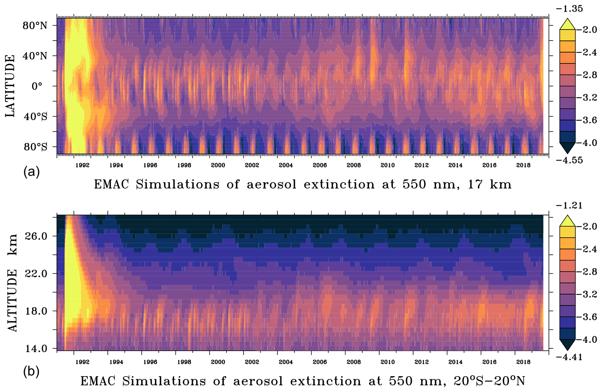
Figure 8EMAC simulation of the stratospheric aerosol extinction on a logarithmic scale log (km−1) for a 550 nm wavelength from January 1991 to August 2019 (5 d averages), zonal mean at 17 km altitude (a) and vertical distribution for tropical regions 20∘ S–20∘ N (b). Maximum and minimum values appear above (yellow) and below (dark blue) the colour keys, respectively.
The EMAC model simulations of the aerosol extinction coefficients at 550 nm (Fig. 8) agree well with the satellite measurements of GOMOS (Fig. 2), SAGE II (Fig. 5), and GloSSAC (Appendix C) for the aerosol layer at an altitude of 16–22 km, where measured extinction values exceed km−1. Above about 24 km EMAC is lower than the observations, likely because in the model meteoric dust particles were not considered.
Figures 7 and 8 show a similar distribution of the aerosol extinction at wavelengths of 550 and 750 nm. Due to the typical size and composition of stratospheric aerosol particles, the aerosol extinction is higher at 550 than at 750 nm. The peaks caused by mineral dust particles during summer in the northern sub-tropics are more pronounced at 750 than at 550 nm.
Despite the presence of volcanoes in the Antarctic (like Mount Erebus), the seasonal change in the extinction coefficient around 80∘ S is not due to volcanic eruptions but to the presence of polar stratospheric clouds (PSCs) as simulated by the model.
6.2 EMAC simulations of AOD
For practical reasons, the total stratospheric AOD is obtained by the vertical integral of the aerosol extinction above an altitude of about 16 km in the tropics and above about 13 km for mid latitudes and high latitudes, to allow for a direct comparison with the existing literature (Santer et al., 2014; Glantz et al., 2014) and satellite data. The stratospheric AOD is shown on a logarithmic scale in Figs. 9 and 10 with the new model simulations (red line) compared to satellite observations (light blue, grey, and blue lines). Using the wavelengths of the satellites in the calculations (Sect. 3) avoids introducing additional errors through the use of conversion factors to adjust the values between the different wavelengths.
From 1991 to 2012, SAGE II (light blue line), GOMOS (grey line), and SAGE + CALIPSO and SAGE + OSIRIS (blue line) provide satellite data at a wavelength of 550 nm (OSIRIS data were converted from 750 nm by Glantz et al., 2014), shown in Fig. 9. For comparison, GloSSAC (Kovilakam et al., 2020) is also included as a black line in the upper panels using the vertical integral over extinction.
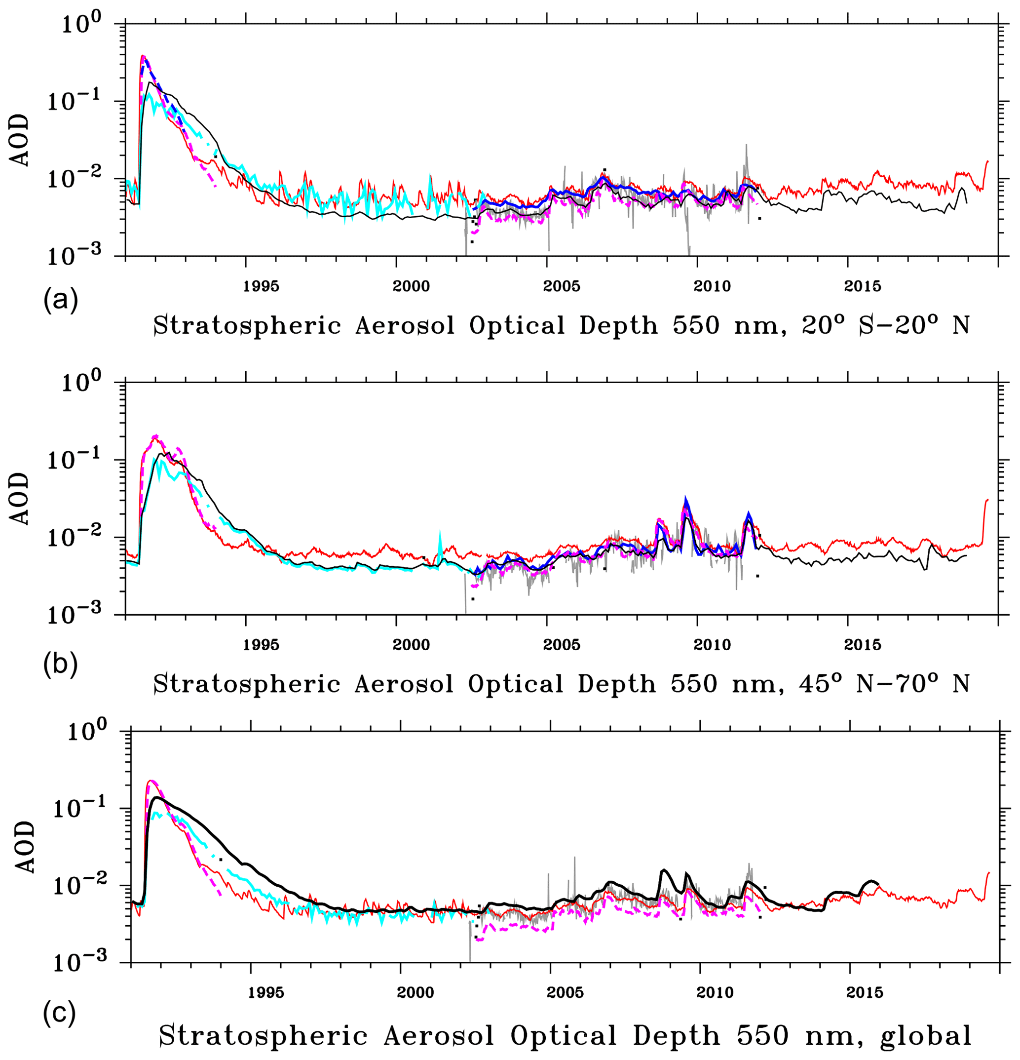
Figure 9Stratospheric AOD at 550 nm wavelength: tropical regions 20∘ S–20∘ N above 16 km are shown in panel (a), the Northern Hemisphere 45–70∘ N above about 13 km in panel (b) and global means in panel (c). Satellite observations from SAGE II (Thomason et al., 2008) are indicated by the light blue line, GOMOS (Bingen et al., 2017) by the grey line and values derived from SAGE + CALIPSO (a) (Santer et al., 2014) and SAGE + OSIRIS (b) (Glantz et al., 2014) by the blue line. The red line shows the EMAC model simulations using the three-dimensional SO2 injections of Table compared to the simulations of Brühl et al. (2015) (pink dashed line) and the global stratospheric AOD from Schmidt et al. (2018) (black line in panel c). The black line in panels (a) and (b) represents GloSSAC, derived from extinction at 525 nm. For the Pinatubo period the dashed blue line shows the AVHRR observations by Long and Stowe (1994) at 630 nm (a). EMAC and GOMOS as 5 d averages, other data monthly.
The maximum is reached after the Pinatubo eruption with a stratospheric AOD of 0.4 in the tropics (Fig. 9, upper panel, EMAC), being an order of magnitude larger than the following medium eruptions with a stratospheric AOD of about 0.01 (e.g. Manam in early 1997, Rabaul in 2006, and Nabro in 2011). The differences after the large Pinatubo eruption in 1991 between the model simulations and the SAGE II observations are related to the “saturation” effects of the satellite instrument (i.e. data gaps due to an opaque path through the atmosphere at the tangent point) and can be observed for more than 1 year, also shown above in Fig. 5. In GloSSAC, gap filling (with lidar and CLAES data) was applied for this case. In this study about 17 Tg SO2 was injected for the Pinatubo eruption (Guo et al., 2004). Model comparisons by Timmreck et al. (2018) show that the span of the used injections varies between 10 Tg SO2 (e.g. Dhomse et al., 2014; Mills et al., 2016; Schmidt et al., 2018) and 20 Tg SO2 (e.g. English et al., 2013). Thus, this study is within the range of the injected sulfur masses. On the other hand, filling the gaps in the SAGE data just by horizontal linear interpolation increases the peak AOD by about a factor of 2, which is close to the GloSSAC compilation. In Fig. 10 the AOD from the AVHRR (Advanced Very High Resolution Radiometer) by Long and Stowe (1994) at 630 nm is included, which is close to our simulations. Consistent with the typical wavelength dependence, these values lie between the red curves for 550 nm (Fig. 9) and 750 nm (Fig. 10) at the peak after the Pinatubo eruption.
When comparing the EMAC simulations (red line in Fig. 9) with the simulation of Schmidt et al. (2018) (black line in Fig. 9c), it can be recognized that a smaller value for the peak of the Pinatubo eruption occurs. Here it needs to be considered that Schmidt et al. (2018) inject less SO2. For Pinatubo, monthly averaging reduces the peak in EMAC by about 5 %, and the smaller events cause fluctuations of up to ±0.007 (see Supplement Fig. S2).
Between 1993 and 1996 the reduction in the stratospheric AOD in the model simulations is faster than indicated by the satellite observations and in Schmidt et al. (2018). This indicates that the removal of stratospheric aerosol is still too rapid when applying our modal model. Schmidt et al. (2018) show a slower decrease in AOD after the Pinatubo eruption. This could indicate that EMAC still needs better fine-tuning of the size distribution modes or addition of modes in the aerosol sub-model to improve the aerosol removal in the stratosphere. Additionally, smaller volcanic eruptions might be missing in view of the low number of identified events in the years after the Pinatubo eruption.
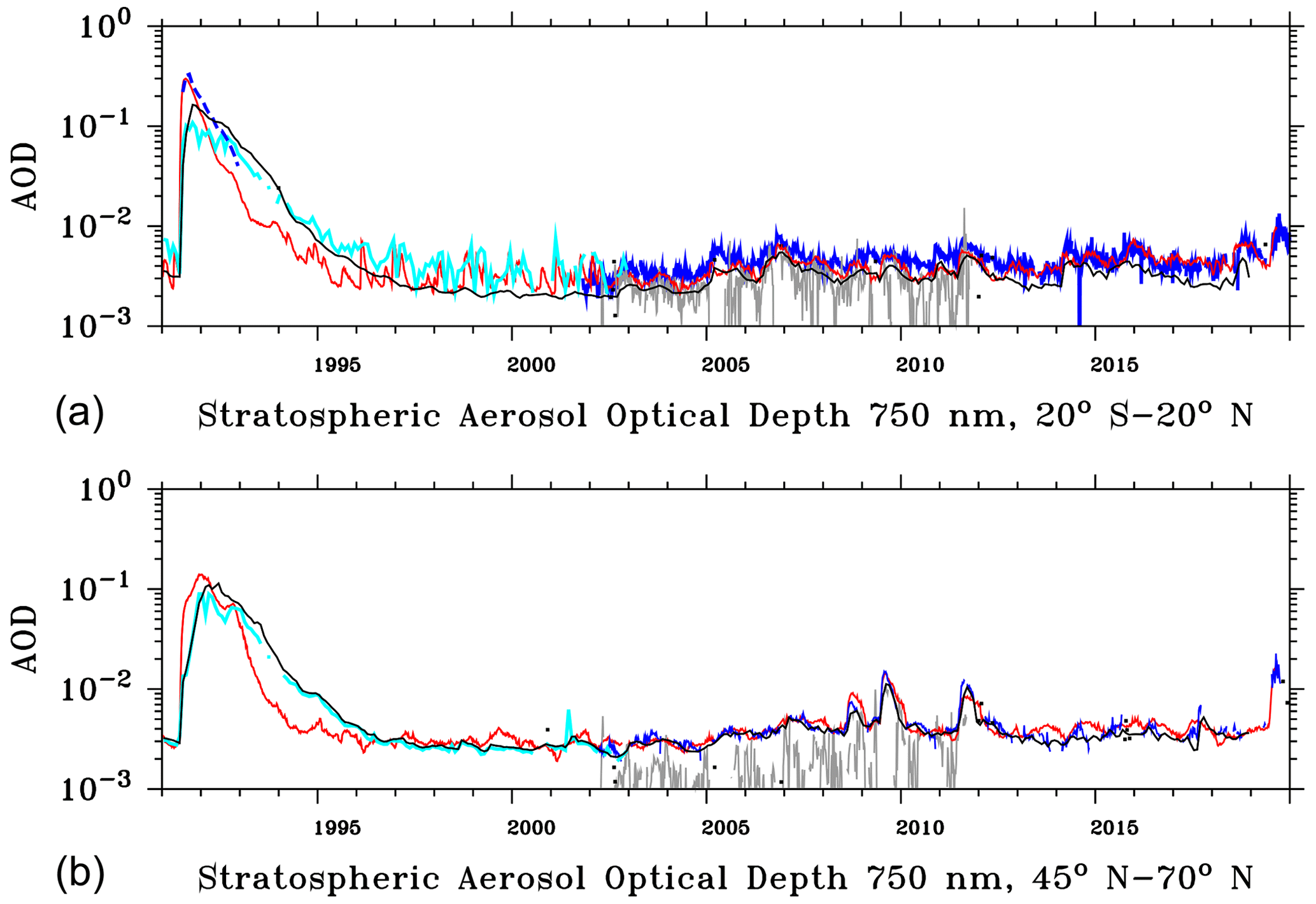
Figure 10Stratospheric AOD at 750 nm wavelength: tropical regions 20∘ S–20∘ N above 16 km are shown in (a) and for the Northern Hemisphere 45–70∘ N above 13 km in (b). Satellite observations from OSIRIS (Rieger et al., 2019) are indicated by the blue line and GOMOS (Bingen et al., 2017) by the grey line. For the Pinatubo period the dashed blue line shows the AVHRR observations by Long and Stowe (1994) at 630 nm (a). The light blue line shows the interpolation of SAGE data at the 525 nm and 1020 nm wavelengths. The EMAC model simulations, using the three-dimensional SO2 injections of Table , are shown by the red line. The black line represents GloSSAC, derived from extinction at 525 and 1020 nm. EMAC, GOMOS, and OSIRIS as 5 d averages, other data monthly.
In Fig. 10, the coverage of GOMOS (grey line) is often too low at a wavelength of 750 nm for the years from 2002 to 2012, so the inclusion of OSIRIS data (blue line) is important (Brühl et al., 2018). For the years after 2012 the timeline only contains data from OSIRIS at the 750 nm wavelength.
Nevertheless, there remain small differences between the model simulation and the observations, for instance in 2010, which indicates missing volcanic eruptions (or an underestimation of the Merapi eruption by MIPAS compared to OSIRIS, Appendix B, or to other data, Mills et al., 2016).
The different distributions of the peaks in the upper and lower panels are related to the latitude of the volcanic eruptions. Emissions reaching the stratosphere from strong eruptions in the tropics are distributed by the Brewer–Dobson circulation over the Northern Hemisphere and Southern Hemisphere even to high latitudes, as in the cases of Soufriere Hills and Rabaul in 2006. However, if an eruption takes place at high latitudes (such as for Redoubt 2009) or at mid latitudes like Kasatochi (2008), Sarychev (2009) or Raikoke (2019), most of the emissions stay in the Northern Hemisphere, and the signal in the tropics is weaker. Our Northern Hemisphere results for AOD (at 550 nm) of about 0.025 after the Raikoke eruption agree within uncertainties with Kloss et al. (2021), who use different satellites and different modelling approaches.
6.3 EMAC simulations comparing the radiative forcing at the top of the atmosphere
The instantaneous radiative forcing of the stratospheric aerosol is calculated by multiple calls of the RAD sub-model (Sect. 3). The simulated global instantaneous radiative forcing in W m−2 of stratospheric aerosol at the top of the atmosphere (TOA) is illustrated in Fig. 11.
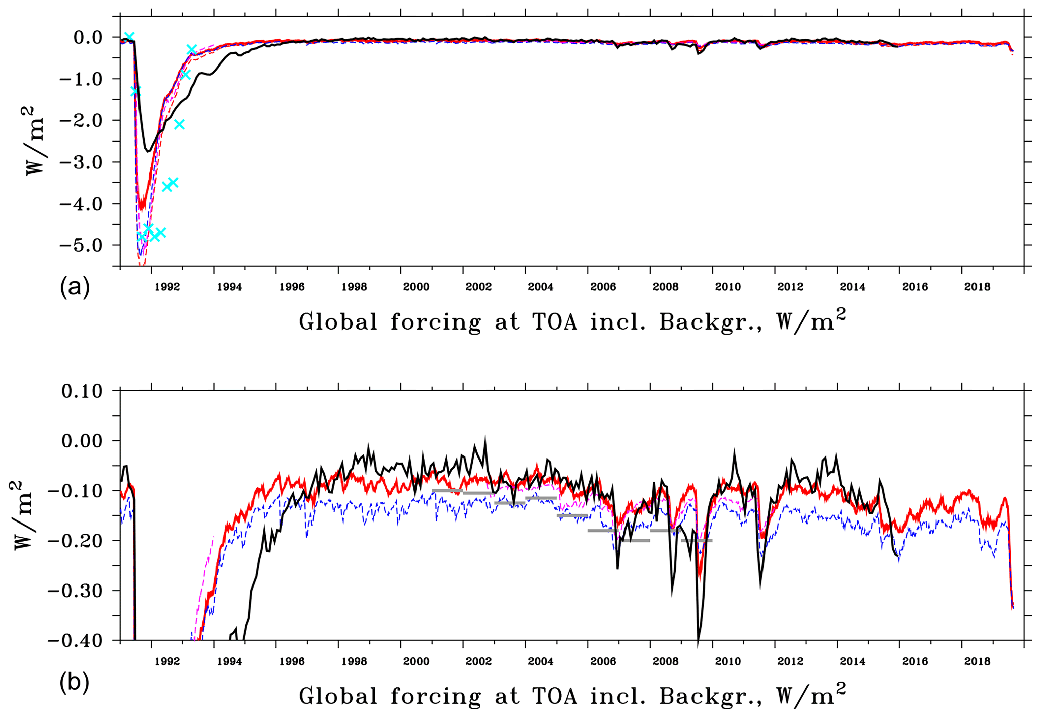
Figure 11EMAC instantaneous radiative forcing by stratospheric aerosol (red, pink, and blue lines, 5 d averages). Solar forcing at the top of the atmosphere (TOA) (dashed red line, a) is compared to solar forcing at the TOA from satellite observations of the Earth Radiation Budget Experiment (ERBE), 72 d means, and light blue crosses (Wong et al., 2006; Toohey et al., 2011). The full red line displays the total (solar + IR) forcing at the TOA, including contributions from aerosol down to the calculated tropopause. The blue dashed line shows the total forcing using the previous scheme at the tropical tropopause (Brühl et al., 2018), the dashed pink line the same with fewer volcanoes of Brühl et al. (2015). Grey bars show annual averages derived from observations by Solomon et al. (2011). The black line shows results from Schmidt et al. (2018) with volcanic effective radiative forcing (aerosol–radiation interactions) at the TOA, including a background aerosol forcing of −0.05 W m−2. Panel (b) is an enhanced representation of panel (a).
As the Pinatubo eruption caused a negative radiative forcing of more than an order of magnitude greater than all other eruptions since then, the figure is sub-divided into two panels with different scalings. The lower panel shows the relatively small values. The new model simulations for the instantaneous radiative forcing at the TOA with the additional volcanic eruptions (red line) are closer to the estimates from satellite extinction measurements of SAGE, GOMOS, and CALIOP by Solomon et al. (2011) (grey bars) than in previous studies (e.g. Brühl et al., 2015, pink dashed line, and Brühl et al., 2018, blue dashed line. For the TOA, see Supplement Fig. S1). In Fig. 11 the published forcing values at the tropical tropopause of the previous studies are shown, which are systematically more negative than the values at the TOA. For Sarychev it is clear that this cannot compensate for the effect of the neglect of aerosol in the extratropical lowermost stratosphere. A comparison with volcanic effective radiative forcing (aerosol–radiation interactions) from Schmidt et al. (2018) is shown by the black line, including a forcing of −0.05 W m−2 for the stratospheric background aerosol (derived from the numbers provided). Especially for high-latitude eruptions their effective forcing (ari) is larger than instantaneous forcing in EMAC and the annual averages of Solomon et al. (2011), also because of a higher aerosol load in the lowermost stratosphere than in EMAC (see sensitivity studies for Sarychev in Appendix C3). In the period considered here, the volcanoes are the dominant factor in (instantaneous) global radiative forcing. Background stratospheric aerosol like sulfate from other sources, dust, and organics contributes about −0.04 W m−2 to the value of the order of −0.1 W m−2 at the TOA in volcanically quiescent periods (e.g. in 2000, 2002, or 2004). At the TOA absolute values up to −0.2 W m−2 (−0.14 W m−2 old approach where only aerosol above 100 hPa was considered) are reached following Rabaul (2006), Kasatochi (2008), Nabro (2011), and Calbuco/Sinabung (2015) and are stronger than −0.32 W m−2 (old approach −0.2 W m−2) following the Raikoke/Ulawun (2019) eruptions. The value for Raikoke/Ulawun is within the range discussed in Kloss et al. (2021).
The strongest instantaneous global radiative forcing in the model simulations is caused by the Pinatubo eruption with a maximum of about −5 W m−2 at the TOA for the solar part (−4 W m−2 for solar + IR forcing at the TOA); this is in good agreement with the results of Minnis et al. (1993) and the observations of the ERBE satellite (light blue crosses in Fig. 11). Schmidt et al. (2018) estimate the effective forcing from the difference of a simulation with and without volcanoes injecting into the stratosphere, i.e. including dynamical and chemical adjustments (effect for Pinatubo up to about 0.4 W m−2). For Pinatubo monthly averaging instead of 5 d averaging reduces the peak by 0.2 W m−2, and the smaller events cause fluctuations of up to ±0.02 W m−2 (i.e. 50 % of the background; see Supplement Fig. S3) at the fine temporal resolution.
6.4 EMAC simulations of the stratospheric aerosol radiative heating
The simulated instantaneous aerosol radiative heating in the model is derived from multiple radiation calls with and without aerosol in the RAD radiation sub-model. Figure 12 shows the calculated local heating effects in the stratospheric aerosol layer. Small and medium volcanic eruptions have the largest effects between altitudes of 17 and 18 km and generate an atmospheric heating of up to 0.03 K d−1. The eruption of Pinatubo, on the other hand, had significantly stronger effects at altitudes of 20 to 25 km and caused atmospheric heating of more than 0.7 K d−1, which corresponds quite well to the results of Rieger et al. (2020) showing a maximum of the instantaneous solar heating rate of 0.5 K d−1 in the tropics near 24 km plus instantaneous thermal heating rates of about 0.2–0.3 K d−1. This is about 23 times greater than all other eruptions in the model simulation, including the Raikoke eruption in 2019.
Further, a seasonal signal contributes significantly to the radiative heating in the northern sub-tropics. This is caused by transport of desert dust to the UTLS, mostly via the Asian summer monsoon convection, which generates additional heating during the time of the Asian summer monsoon (Brühl et al., 2018).
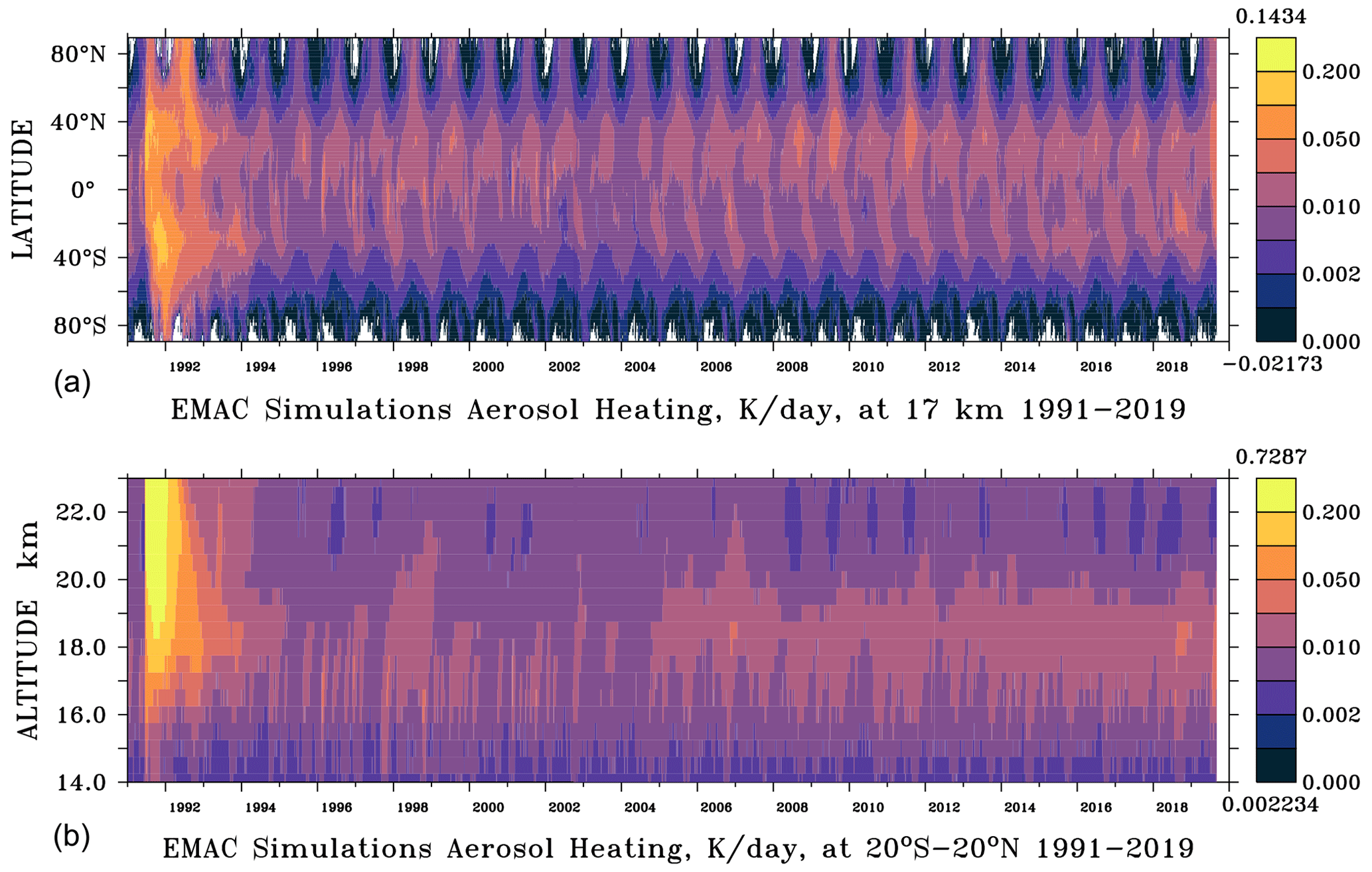
Figure 12EMAC simulation of the aerosol radiative heating in K d−1 for solar and infrared radiation from January 1991 to August 2019 (5 d averages) based on the volcanic sulfur emission inventory (Table ), in horizontal distribution at 17 km altitude (a) and in vertical distribution for tropical regions 20∘ S–20∘ N (b).
The objective of this study was to generate a detailed volcanic sulfur emission inventory and to improve the EMAC model simulations of the global stratospheric aerosol and sulfate burden and compute the long-term volcano-induced instantaneous radiative forcing using computed extinctions validated on the basis of satellite data.
The presented approach, based on observed three-dimensional perturbations of SO2 or extinction due to volcanic eruptions, avoids uncertainties related to the point source approach due to required additional assumptions and possible numerical artifacts related to the extreme perturbations by several orders of magnitude in small regions and non-linear feedback processes. Our case studies on this show large uncertainty in computed instantaneous radiative forcing and the possible development of spurious long-lived mesoscale vortices containing very high sulfate. In our approach the largest uncertainties are due to the handling of gaps in the satellite data.
Updated OSIRIS data allowed us to extend the comparisons of Brühl et al. (2018) to the year 2019; a detailed analysis of Level-2 SAGE II data (individual profiles of extinction at two wavelengths and SAD) together with the Smithsonian volcano database was used to extend the comparison back to 1990. As a result, the simulations in this paper encompass a total of 29 years and cover the period 1991 to 2019 compared with 2002 to 2012 in our previous work. The temporal resolution is 5 d for the three instruments MIPAS, GOMOS, and OSIRIS, and it is possible to identify multiple volcanic eruptions within a short period of time. With the three-dimensional datasets, the vertical distribution of SO2 can be distinguished and the amount of sulfur reaching the stratosphere can be calculated much more accurately than by estimation from a total column. Tropospheric sulfur emissions are treated separately.
Our volcanic sulfur emission inventory is an extension and improvement of the versions published by Bingen et al. (2017) and Brühl et al. (2018). While the previous version included 230 explosive volcanic eruptions, the new version includes more than 500 eruptions. An overview of these eruptions is given in the volcanic sulfur emission inventory in Table , which indicates the estimated stratospheric SO2 emissions as well as the plume altitudes. These consist of about 80 eruptions in the first time period between 1990 and 2002 measured by the SAGE II instrument, 240 eruptions in 2002–2012 measured with multiple instruments, and 230 eruptions in the last time period 2012–2019 measured by OSIRIS. The consequence of the inclusion of many more small-sized eruptions reaching the UTLS is that stratospheric aerosol optical depth and radiative forcing do not decrease to the non-volcanic background between medium-sized eruptions, in agreement with observations.
Strong volcanic eruptions can inject several teragrams of SO2 directly into the stratosphere. For this reason, the maxima of the global stratospheric SO2 concentrations correlate well with the eruption events of the volcanic sulfur emission inventory in Table . The SO2 emissions of smaller volcanic eruptions can reach the lower stratosphere by convective transport through the tropical tropopause, which results in accumulation of sulfate aerosol in the lower stratosphere. This was demonstrated to be important for correctly modelling the AOD in volcanically quiescent periods.
Our analysis shows the importance of using multi-instrument satellite datasets to fill data gaps and to detect as many volcanic eruptions as possible. The optimal data coverage time period is from 2002 to 2012, for which simultaneous measurements from the MIPAS, GOMOS, and OSIRIS instruments are available. For 2002 to 2005 this also includes SAGE II. The periods with simultaneous observations by MIPAS and the other instruments were used to develop and validate a method for estimating injected SO2 and its distribution from extinction observations. The evaluation by the satellite datasets shows that GOMOS is important for detecting volcanic eruptions during MIPAS data gaps and for a better attribution of individual eruptions. Consequently, the combination of MIPAS, GOMOS, and OSIRIS data leads to an improved SO2 emission database for calculating the instantaneous radiative forcing in the EMAC chemistry-climate model.
Large volcanic ash plumes can interfere with the SO2 signal in satellite measurements, and satellites could be “blind” during the first few days or months after an eruption (Höpfner et al., 2015). However, most volcanic ash particles are relatively large and sediment after some hours or days, and hence they only have minor climatic significance (Boucher, 2015) and are not discussed in detail here. There are, however, volcanoes (e.g. the eruption of Kelut in 2014; Zhu et al., 2020) which emitted small ash particles which can stay in the lower stratosphere for several months (Vernier et al., 2016). Moreover, we found that the model set-up might have to be improved by including an additional aerosol mode to reduce the removal by sedimentation of stratospheric aerosol after large volcanic eruptions. Some satellite datasets are affected by gaps and noise. Comparing the model results with OSIRIS data in the tropics (Fig. 10) indicates that some volcanic events are underestimated or missing in the volcanic sulfur emission inventory in the year 2010.
Frequent volcanic eruptions of moderate and small intensities, injecting sulfur gases into the upper troposphere and lower stratosphere, contribute significantly to the stratospheric aerosol layer, in particular through their accumulation in time. These cause a global negative instantaneous radiative forcing of the order of more than 0.1 W m−2 at the TOA, including a background aerosol forcing of about 0.04 W m−2. For example, after the eruptions of Soufriere Hills/Rabaul (2006) and Nabro (2011) and the combination of the Sinabung, Wolf, and Calbuco eruptions (2015), a negative instantaneous radiative forcing of 0.2 W m−2 (0.14 W m−2, old approach) and 0.32 W m−2 (0.2 W m−2, old approach) was reached after Raikoke/Ulawun (2019) at the TOA.
Note that for the calculation of the instantaneous forcing by these medium-sized eruptions, it is essential to consider the radiative effect of volcanic aerosol down to the tropopause (Ridley et al., 2014). Including only the aerosol above the 100 hPa level as done in Brühl et al. (2018, 2015) can lead to significant underestimates which were partially hidden in these studies by showing the instantaneous forcing at the tropopause which is about 0.08 W m−2 stronger than at the TOA in EMAC.
The model also includes mineral dust and organics transported from the lower troposphere to the UTLS. The EMAC simulations show a seasonal signal in the stratospheric AOD and an enhanced radiative heating in the Northern Hemisphere induced by the convective transport of mineral dust to the UTLS in the Asian monsoon region. This is confirmed by satellite observations and by Klingmüller et al. (2018). The influence of wildfires and other biomass burning plumes on stratospheric AOD has increased in recent years (Fromm et al., 2019), and this effect should be included in the model to account for perturbations in organic and black carbon.
The computations for this study were performed on the Mistral supercomputer at the Deutsches Klimarechenzentrum (DKRZ), Hamburg, Germany. For this purpose, EMAC (ECHAM5/MESSy Atmospheric Chemistry), a coupled atmospheric circulation model consisting of the 5th generation of the European Centre Hamburg general circulation model (ECHAM5) and the MESSy (V2.52), was used.
ECHAM5 (5th generation of the European Centre Hamburg general circulation model) is an atmospheric general circulation model (Roeckner et al., 2003, 2006), which runs with the self-consistent quasi-biennial oscillation (QBO). It is nudged to the meteorological ERA-Interim reanalysis data of the European Centre for Medium-Range Weather Forecasts (ECMWF) up to about 100 hPa. To avoid a phase drift, we used the QBO sub-model for weak nudging to the QBO zonal wind observations (Giorgetta et al., 2002).
MESSy is an Earth system model, which consists of several sub-models (Jöckel et al., 2005, 2006, 2010). An overview of the sub-models used in this study is given in Table A1.
Mineral dust emissions are calculated online using the emission scheme of Astitha et al. (2012) as part of the ONEMIS sub-model. The sub-model TREXP (Jöckel et al., 2010) is needed to inject SO2 emissions in point source emission simulations. The convection was calculated with the CONVECT sub-model (Tost et al., 2006b), with the convection scheme from Tiedtke (1989) and the Nordeng (1994) closure. The convection parametrization is sensitive to the model resolution, which results in differences between different model resolutions in the vertical transport of tracers, like dust, water vapour, ozone, and SO2, especially near the low-latitude tropopause (Brühl et al., 2018).
The loss of gas-phase species to the aerosol is parameterized in the third EQuilibrium Simplified Aerosol Model (EQSAM3) (Metzger and Lelieveld, 2007). The uptake of gases on wet particles and on acid aerosol particles is included in the model calculation. Concerning removal mechanisms, the SCAVenging sub-model calculates the loss of atmospheric tracers and aerosols by wet deposition as well as the liquid-phase chemistry in clouds and precipitation (Tost et al., 2006a). The chemistry of the CAABA/MECCA sub-model contains photolysis reactions, which need photolysis rate coefficients (J values) for tropospheric and stratospheric species computed by the JVAL sub-model. The RAD_FUBRAD sub-sub-model is used to calculate the short-wave heating rates from the absorption of UV by O2 and O3 in the upper stratosphere and mesosphere. The lowermost level of the RAD_FUBRAD sub-sub-model for the upper atmosphere is shifted from above 70 hPa in the original version of Dietmüller et al. (2016) to 30–14 hPa to allow for scattering by the aerosol in the simulations with volcanic emissions.
Dietmüller et al. (2016)Pozzer et al. (2006)Sander et al. (2011)Tost et al. (2006b)Tost et al. (2010)Kerkweg et al. (2006a)Pringle et al. (2010)Jöckel et al. (2006)Jöckel et al. (2006)Tost et al. (2007)Jöckel et al. (2010)Kerkweg et al. (2006b)Kerkweg et al. (2006b)Giorgetta et al. (2002)Dietmüller et al. (2016)Tost et al. (2006a)Kerkweg et al. (2006a)Kerkweg et al. (2006b)Jöckel et al. (2010)Jöckel et al. (2006)Table A1List of MESSy sub-models used. References and short description from https://messy-interface.org/messy/submodels/ (last access: 10 January 2023). Parts of the base model copied into MESSy which must always be active are not listed here.

The eruption of Reventador in the tropics in November 2002 has been shown to be an ideal case where simultaneous observations of all satellite sensors were available, so that the direct SO2 observation could be used for development and validation of a conversion formula for the 750 nm extinction seen by GOMOS and OSIRIS, which also works approximately for SAGE if its observations at 525 and 1020 nm are interpolated to 750 nm. Here we first use the ratio between the model-calculated sulfate volume mixing ratio and its share in extinction at low latitudes of the lower stratosphere, which is typically 1.2×10¹² per air density (molec. cm−3) for the period during which MIPAS was available. This works for medium- and small-sized eruptions and data available over about 4 weeks following the eruptions and if no other events occur less than about 4 weeks before, which is the case for the Reventador eruption. If the time lag of data is several weeks, a correction factor of >1 has to be applied in Eq. (1) to account for removal processes, and if another event is relatively close in time, the factor has to be <1 to remove the influence of the previous event (see Tables S1 and S2 in the Supplement, which also indicate additional uncertainties for a few cases in 2018 and 2019 due to too sparse data).
For Reventador the factor is 1 for all instruments (for OSIRIS 0.8 is slightly better because of remnants from the Ruang eruption about 4 weeks before). For all instruments the derived injected SO2 mass is very close to 77 kt as shown in Table . The spatial patterns are similar, except that the zonal wind causes a shift in longitude due to the time lag from conversion of SO2 to aerosol; see Fig. B1. In the case of SAGE, the alternative method of Grainger et al. (1995) involving aerosol surface area density (SAD) and aerosol volume density is more suitable for removing cloud perturbation and is used in the simulation. It is assumed that sulfate mixing ratios correspond to the SO2 injected. Some uncertainty remains from removing the background, which we have done by subtracting a fraction of the derived SO2 at the longitude where it has a minimum, i.e. the longitude where the effect of the volcano is smallest for all altitudes. If the extinctions at 525 and 1020 nm are used directly, the patterns are similar except for the lowermost part which contains more data gaps. This has also been checked for every event prior to MIPAS. Integrated injected SO2 masses for all examples are provided in Table B1.
For the eruption of Merapi in November 2010 the satellite instruments do not agree. From OSIRIS about 70 % more injected SO2 is derived than from MIPAS, i.e. 170 kt instead of 97 kt used in the transient simulation (see Table and differences in Fig. 10). GOMOS has too sparse data here to obtain a proper integral directly, but patterns are similar (Fig. B2). If other information is available, the gaps can be filled with likely values in the region where the plume was seen, a method which had to also be applied to some events seen by OSIRIS in 2018 and 2019 for which the data were sparse.
For high-latitude eruptions the longer conversion time of SO2 to sulfate compared to the tropics has to be considered, which, together with aerosol removal processes, leads to a weaker extinction signal. To account for this a correction factor of about 2 in the conversion formula for OSIRIS, for example for Sarychev in June 2009, leads to values consistent with the ones derived by MIPAS (Fig. B3). For the low-latitude eruption of Manda Hararo in the same entry of Table (separated at 24∘ N for the integration), the factor of 1 is still appropriate.
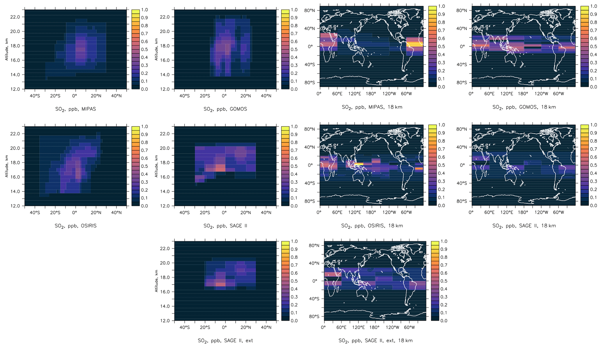
Figure B12002 Reventador eruption: SO2 mixing ratio perturbation (ppb) derived from MIPAS and the three extinction instruments. MIPAS data of 7 to 17 November 2002, OSIRIS and GOMOS data of 11 to 22 November, and SAGE II orbits of November and early December 2002. Zonal average vertical distribution (left) and plumes at 18 km altitude (right). OSIRIS with a correction factor of 0.8 due to remnants from the Ruang eruption and SAGE II with the Grainger-based method. Lower row: SAGE II SO2 derived from extinction (interpolated to 750 nm from 525 and 1020 nm). Factor 1 is the default.
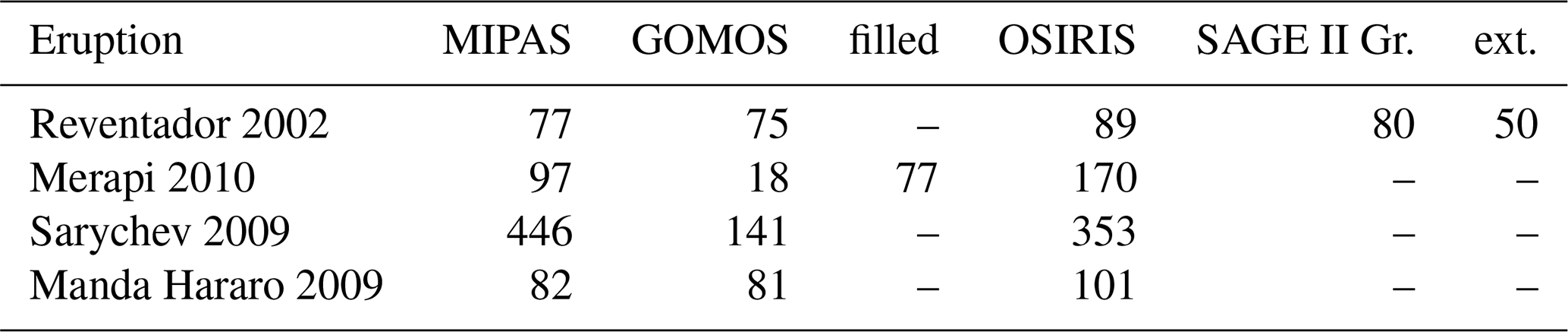

Figure B22010 Merapi eruption: SO2 mixing ratio perturbation (ppb) derived from MIPAS, GOMOS OSIRIS and GOMOS with gap filling. MIPAS data 5 to 20 November 2010, OSIRIS 14 to 25 November, and GOMOS 25 November to 9 December (sparse data). Zonal average vertical distribution (left) and plumes at 18 km altitude (right).
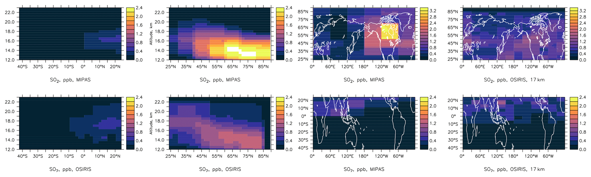
Figure B32009 Sarychev (second column, upper right row) and Manda Hararo (first column, lower right row) eruptions: SO2 mixing ratio perturbation (ppb) derived from MIPAS and OSIRIS; arrangement of the panels because the event is split at 24∘ N as for integrated values in Table . MIPAS data 18 June to 18 July 2009, OSIRIS data 17 July to 3 August. Zonal average vertical distribution (left) and plumes at 17 km altitude (right).
C1 Comparison with GloSSAC
Figure C1 shows the aerosol extinction of GloSSAC on the same logarithmic scale log (km−1) as the used satellite datasets and the EMAC simulations in Figs. 2–8.
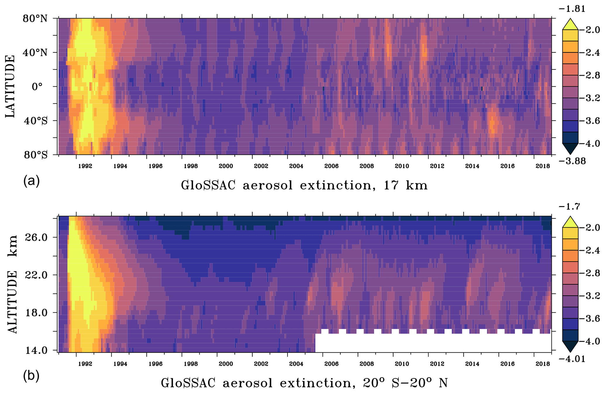
Figure C1GloSSAC aerosol extinction on a logarithmic scale log (km−1) for the 525 nm wavelength from the January 1991–December 2018 zonal mean at 17 km altitude (a) and in vertical distribution for tropical regions 20∘ S–20∘ N (b). Maximum and minimum values appear above (dark red) and below (violet) the colour keys, respectively. White: no data.
C2 Comparison of different volcanic injection inventories
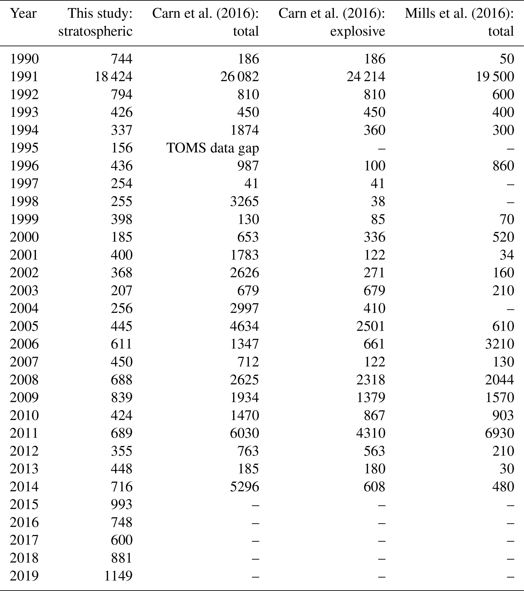
Table C1 shows a comparison of annual volcanic SO2 emission inventories from Carn et al. (2016) and Mills et al. (2016) with this study.
Carn et al. (2016)Carn et al. (2016)Mills et al. (2016)Table C1Comparison of different volcanic emission inventories (annual SO2 – kt): volcanic SO2 emissions reaching the stratosphere and the uppermost tropical troposphere from the Volcanic Sulfur Emission Inventory (Table ) in this study, ending in August 2019 (+ about 19 MtSO2 yr−1 from degassing into the troposphere, Diehl et al., 2012); total annual amount and explosive annual amount of global volcanic SO2 emissions, calculated from satellite observations in 1979 to 2014 by Carn et al. (2016, their Table 3) and total SO2 emissions from Mills et al. (2016, their Table S4).
C3 Comparison with different case studies for volcanic “point source” injections
To compare the simulations from this study using volcanic SO2 as a spatially resolved SO2 cloud instead of the traditional point source approach, some case studies are shown in this chapter. For this purpose, simulations are performed with the same model set-up and with point source injections using the TREXP (Jöckel et al., 2010) sub-model. As case studies we compare different point source injection methods of volcanic SO2 emissions with the EMAC model simulations using the three-dimensional perturbations and MIPAS Level-2 observations for the Nabro eruption in 2011 and the Sarychev eruption in 2009.
To ensure identical boundary conditions, the point source simulations were started using the identical model set-up, and only the volcanic SO2 injections differ from those performed in this study. In contrast to the method used in this study, the point source methods always require, additionally to injected total SO2 mass derived from nadir instruments, assumptions about the altitude range and the duration of the eruption and also the area of the initial plume. In the examples we use the settings of Mills et al. (2016) and the corresponding entries in Table . For the latter we assume as one option that the SO2 mass is injected equally distributed between the latitude-dependent lower minimum altitude given in the caption, and approximately the listed altitude of the maximum perturbation of the mixing ratio, the injection time, and the duration is assumed to be the same as in Mills et al. (2016) or, if missing, in the Smithsonian database. Alternatively we assume that emissions begin about 1.2 km (two to three model layers) above the minimum altitude.
We compare zonal average vertical distributions of SO2 (Fig. C2) and sulfate (Fig. C3) some weeks after the eruptions for the Sarychev eruption in 2009 (left) and the Nabro eruption in 2011 (right). In the case of using the three-dimensional SO2 perturbations, the resulting SO2 distribution is smoother than with direct use of Table for “point sources”. Using Mills “point sources” shifts the SO2 plume to lower altitudes.
Five-day-average radiative forcing at the TOA is shown in Fig. C4. The black curves correspond to the red curves in Fig. 11. Using the assumptions of Mills et al. (2016) about the vertical distribution of the SO2 injection leads to less forcing in the case of Nabro and after about 5 weeks after the Sarychev eruption (Fig. C4, red curves). For the latter the peak is stronger since more mass is injected than in the other approaches. It is dominated by contributions from aerosol in the mid- and high-latitude lowermost stratosphere. Using Table leads to approximate agreement if the provided altitude is about the top of the column into which it is injected, using as a bottom about 1.2 km above the latitude-dependent minimum altitude (blue curves). Using the full range leads to an underestimate compared to the simulation using the MIPAS observations directly as three-dimensional SO2 perturbation (light blue curves). This is due to more efficient removal processes in the upper troposphere and the lowermost stratosphere than in the layers above. The lower panel for 2009 also contains a sensitivity study similar to the blue curve but with the eruption of Manda Hararo neglected as done by Mills et al. (2016) (dashed) and one where the top of the injection column for Sarychev was one layer lower than in the case with the light blue curve (purple). These examples show that the altitude of the injection has a large impact on the radiative forcing but also that not only medium-sized eruptions matter. For stratospheric AOD shown in the upper panels of Fig. C4 the difference between the approaches is less than for the forcing in the first weeks after the eruption. Later the SAOD decreases faster with the point source approach, especially the one of Mills et al. (2016), than with our method.
Note that considering only aerosol above the fixed pressure level of 100 hPa for the forcing calculations as we did in earlier studies causes misleading results here.
We further show maps at 16 and 18 km altitude and the corresponding Level-2 MIPAS observations (see Figs. C5 to C6). In the case of Nabro using column emissions of up to about 18 km interaction of chemistry, radiative heating, and dynamics leads to the formation of a lofting anti-cyclonic vortex with elevated concentrations of SO2 and sulfate above 18 km, propagating westward for several weeks. In Fig. C6 this is visible over the sub-tropical eastern Pacific but is not supported by observations in this case. The phenomenon appears to be similar to the one observed after the 2019/2020 wildfires over the South Pacific (Khaykin et al., 2020).
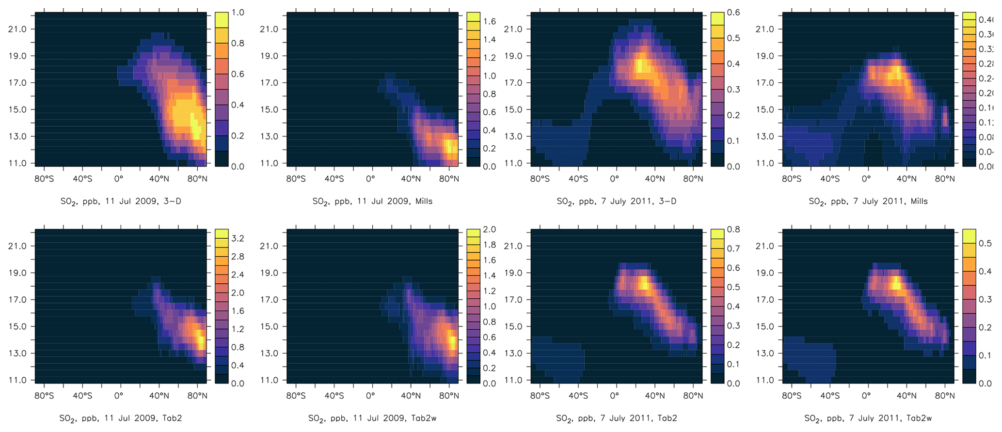
Figure C2Zonal average SO2 mixing ratio (ppb) distribution with latitude and altitude (km), 11 July 2009 (four left panels) and 7 July 2011 (four right panels). “3-D” this study, “Mills” emission settings of Mills et al. (2016), “Tab2w” emission in full columns of Table , “Tab2” emission starting about 1.2 km above the minimum altitude of Table .
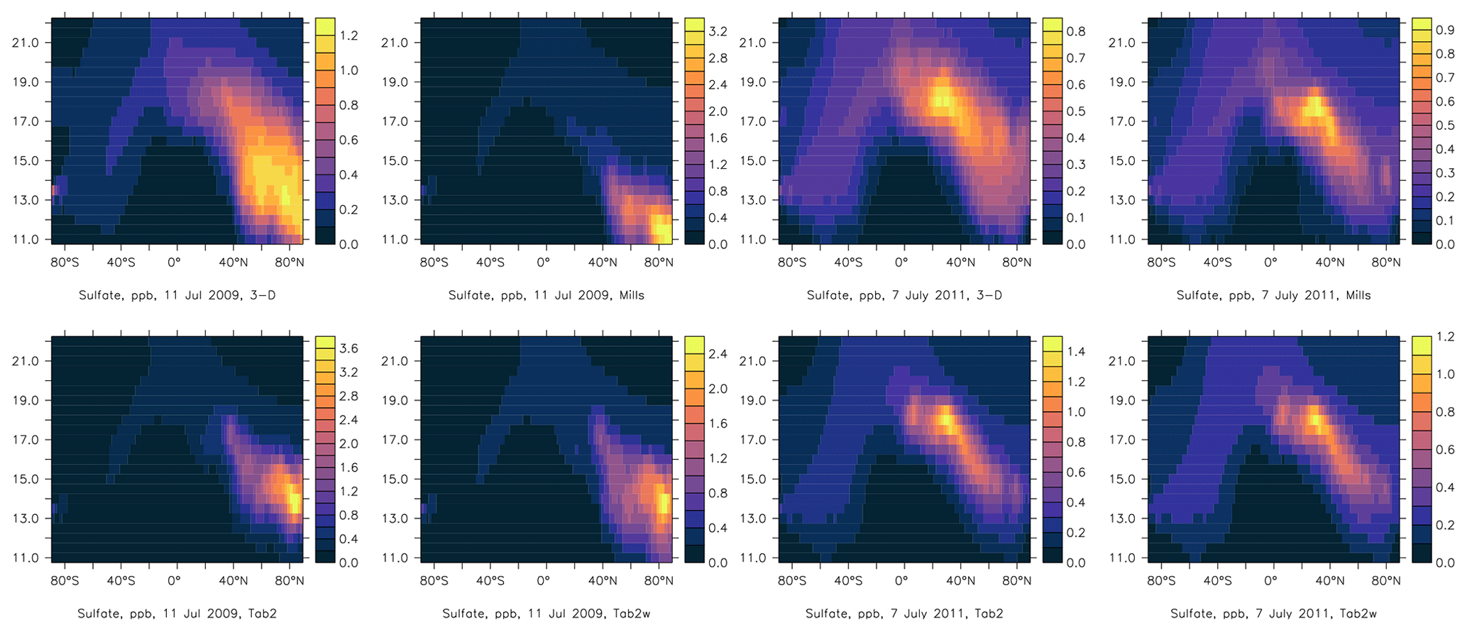
Figure C3Like Fig. C2 but for sulfate in the accumulation mode.
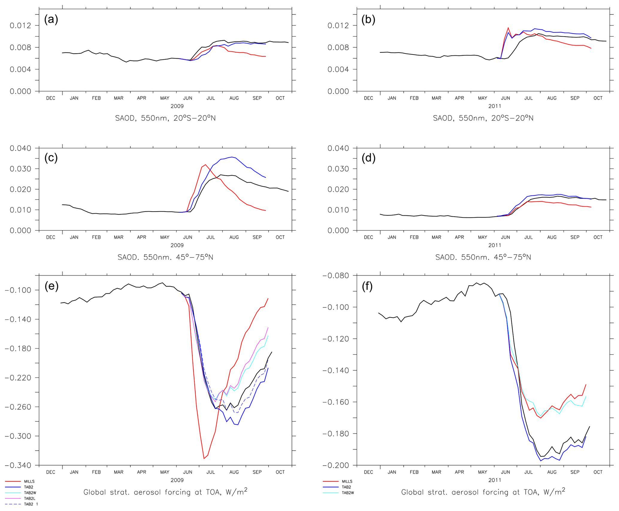
Figure C4Stratospheric AOD (a–d) and global radiative forcing at the TOA (e, f), Sarychev (a, c, e) and Nabro (b, d, f), black line like the red line in Figs. 9 or 11, blue, light blue and purple line “point sources” based on Table with different thicknesses and vertical positions of the column into which this is injected (see text), and red lines with the assumptions of Mills et al. (2016). Dashed blue, light blue, and purple curves: see text.

Figure C5SO2 mixing ratio (ppb) maps after the Sarychev eruption at 16 km (left column) and 18 km (right column) for point sources of Table in the column between 15 and 17 km (first row), the column between 13 and 17 km (second row), our three-dimensional approach (third row) and the point source assumption of Mills et al. (2016) with a column below 15 km (Manda Hararo neglected) (fourth row). Bottom row from MIPAS observations.

Figure C6SO2 mixing ratio (ppb) maps after the Nabro eruption at 16 km (left column) and 18 km (right column) for the point source of Table in the column between 15.5 and 18 km (first row), the column between 14 and 18 km (second row), our three-dimensional approach (third row) and the point source assumption of Mills et al. (2016) with a column below 16 km (fourth row). Bottom row from MIPAS observations.
The Modular Earth Submodel System (MESSy) is continuously developed and used by a consortium of institutions. The use of MESSy and access to the source code is licensed to all affiliates of institutions which are members of the MESSy consortium. Institutions can become a member of the MESSy consortium by signing the MESSy Memorandum of Understanding. More information can be found on the MESSy consortium website (https://messy-interface.org, last access: 21 December 2022). The code used here is based on MESSy version 2.52 stored at DKRZ and available from the authors on request. The input data files and model output of EMAC used here are stored at DKRZ, Hamburg, the volcanic inventory and the output for instantaneous radiative forcing at tropopause also at WDCC (https://doi.org/10.26050/WDCC/SSIRC_3, Brühl et al., 2021). For the MIPAS data we refer to http://www.imk-asf.kit.edu/english/308.php (MIPAS, 2023). A detailed documentation on the used data for MIPAS, SAGE, OSIRIS and GOMOS for the individual events is available from the authors on request.
The supplement related to this article is available online at: https://doi.org/10.5194/acp-23-1169-2023-supplement.
JS, CBr and JL defined the scientific questions and scope of this work. JS and CBr conceived the idea and methodology used in this paper and carried out the model simulations and the analysis. MH provided the MIPAS data, CBi provided the GOMOS data, and LR provided the OSIRIS data. All the authors participated in the scientific discussion in regard to satellite data in particular. JS wrote the manuscript, and all the authors reviewed the manuscript and provided advice on the manuscript and figures.
The contact author has declared that none of the authors has any competing interests.
Publisher's note: Copernicus Publications remains neutral with regard to jurisdictional claims in published maps and institutional affiliations.
This article is part of the special issue “The Modular Earth Submodel System (MESSy) (ACP/GMD inter-journal SI)”. It is not associated with a conference.
There is a close collaboration within the SPARC/SSIRC (Stratosphere-troposphere Processes And their Role in Climate/Stratospheric Sulfur and its Role in Climate) stratospheric aerosol model intercomparison project (http://www.sparc-ssirc.org, last access: 21 December 2022) concerning SO2 injections derived from satellite data and model intercomparisons. Many thanks to Matthias Kohl for helping to set up the additional point-source emission simulations. The computations have been performed at the Mistral and Levante supercomputers at DKRZ, Hamburg, Germany. We thank Adam Bourassa, Larry Thomason and the GOMOS, MIPAS, OSIRIS, SAGE, the Copernicus Climate Change Service (projects C3S_312a_Lot5 and C3S_312b_Lot2), and EOSDIS (NASA) teams for their productive cooperation and providing their satellite datasets. GloSSAC (V2) data were obtained from the NASA Langley Research Center – Atmospheric Sciences Data Center. For the SO2 inventory we also utilized the NASA SO2 database at GSFC (http://so2.gsfc.nasa.gov, last access: 21 December 2022) for OMI and TOMS and the Smithsonian volcano database (http://www.volcano.si.edu, last access: 21 December 2022) We are grateful to our colleagues from the EMAC community and all other MESSy developers and users for their support. We thank Anja Schmidt for editing our paper and providing the data of her paper for comparisons with our results. We would also like to thank the referees for their comments to help us improving our paper.
The research leading to these results has received funding from the European Research Council under the European Union's Seventh Framework Programme (FP7/2007–2013)/ERC grant agreement 226144 as part of the StratoClim project and funding from ESA Aerosol CCI (European Space Agency).
The article processing charges for this open-access
publication were covered by the Max Planck Society.
This paper was edited by Anja Schmidt and reviewed by Thomas Aubry and two anonymous referees.
Andersson, S. M., Martinsson, B. G., Vernier, J.-P., Friberg, J., Brenninkmeijer, C. A. M., Hermann, M., van Velthoven, P. F. J., and Zahn, A.: Significant radiative impact of volcanic aerosol in the lowermost stratosphere, Nat. Commun., 6, 7692, https://doi.org/10.1038/ncomms8692, 2015. a
Aquila, V., Oman, L. D., Stolarski, R. S., Colarco, P. R., and Newman, P. A.: Dispersion of the volcanic sulfate cloud from a Mount Pinatubo-like eruption, J. Geophys. Res.-Atmos., 117, D06216, https://doi.org/10.1029/2011JD016968, 2012. a
Astitha, M., Lelieveld, J., Abdel Kader, M., Pozzer, A., and de Meij, A.: Parameterization of dust emissions in the global atmospheric chemistry-climate model EMAC: impact of nudging and soil properties, Atmos. Chem. Phys., 12, 11057–11083, https://doi.org/10.5194/acp-12-11057-2012, 2012. a
Aubry, T. J., Staunton-Sykes, J., Marshall, L. R., Haywood, J., Abraham, N. L., and Schmidt, A.: Climate change modulates the stratospheric volcanic sulfate aerosol lifecycle and radiative forcing from tropical eruptions, Nat. Commun., 12, 1–16, https://doi.org/10.1038/s41467-021-24943-7, 2021. a
Bertaux, J. L., Kyrölä, E., Fussen, D., Hauchecorne, A., Dalaudier, F., Sofieva, V., Tamminen, J., Vanhellemont, F., Fanton d'Andon, O., Barrot, G., Mangin, A., Blanot, L., Lebrun, J. C., Pérot, K., Fehr, T., Saavedra, L., Leppelmeier, G. W., and Fraisse, R.: Global ozone monitoring by occultation of stars: an overview of GOMOS measurements on ENVISAT, Atmos. Chem. Phys., 10, 12091–12148, https://doi.org/10.5194/acp-10-12091-2010, 2010. a, b
Bingen, C., Robert, C. E., Stebel, K., Brühl, C., Schallock, J., Vanhellemont, F., Mateshvili, N., Höpfner, M., Trickl, T., Barnes, J. E., Jumelet, J., Vernier, J.-P., Popp, T., de Leeuw, G., and Pinnock, S.: Stratospheric aerosol data records for the climate change initiative: Development, validation and application to chemistry-climate modelling, Remote Sens. Environ., 203, 296–321, https://doi.org/10.1016/j.rse.2017.06.002, 2017. a, b, c, d, e, f, g, h, i, j, k, l
Bingen, C., Robert, C., Hermans, C., Vanhellemont, F., Mateshvili, N., Dekemper, E., and Fussen, D.: A Revised Cross-Section Database for Gas Retrieval in the UV-Visible-Near IR Range, Applied to the GOMOS Retrieval Algorithm AerGOM, Front. Environ. Sci., 7, 1–18, https://doi.org/10.3389/fenvs.2019.00118, 2019. a
Boucher, O.: Atmospheric Aerosols, Springer Netherlands, Dordrecht, https://doi.org/10.1007/978-94-017-9649-1, 2015. a
Bourassa, A. E., Rieger, L. A., Lloyd, N. D., and Degenstein, D. A.: Odin-OSIRIS stratospheric aerosol data product and SAGE III intercomparison, Atmos. Chem. Phys., 12, 605–614, https://doi.org/10.5194/acp-12-605-2012, 2012a. a, b, c
Bourassa, A. E., Robock, A., Randel, W. J., Deshler, T., Rieger, L. A., Lloyd, N. D., Llewellyn, E. J., and Degenstein, D. A.: Large volcanic aerosol load in the stratosphere linked to Asian monsoon transport, Science, 336, 78–81, https://doi.org/10.1126/science.1219371, 2012b. a
Brühl, C.: Volcanic SO2 data derived from limb viewing satellites for the lower stratosphere from 1998 to 2012, and from nadir viewing satellites for the troposphere, World Data Center for Climate (WDCC) at DKRZ [data set], https://doi.org/10.1594/WDCC/SSIRC_1, 2018. a
Brühl, C., Lelieveld, J., Tost, H., Höpfner, M., and Glatthor, N.: Stratospheric sulfur and its implications for radiative forcing simulated by the chemistry climate model EMAC, J. Geophys. Res., 120, 2103–2118, https://doi.org/10.1002/2014JD022430, 2015. a, b, c, d, e, f, g, h
Brühl, C., Schallock, J., Klingmüller, K., Robert, C., Bingen, C., Clarisse, L., Heckel, A., North, P., and Rieger, L.: Stratospheric aerosol radiative forcing simulated by the chemistry climate model EMAC using Aerosol CCI satellite data, Atmos. Chem. Phys., 18, 12845–12857, https://doi.org/10.5194/acp-18-12845-2018, 2018. a, b, c, d, e, f, g, h, i, j, k, l, m, n, o, p, q
Brühl, C., Schallock, J., and Diehl, T.: Volcanic SO2 data derived from limb viewing satellites for the lower stratosphere from 1990 to 2019, and from nadir viewing satellites for the troposphere, including the corresponding radiative forcing computed by the CCM EMAC, World Data Center for Climate (WDCC) at DKRZ [data set], https://doi.org/10.26050/WDCC/SSIRC_3, 2021. a, b
Carn, S. A., Clarisse, L., and Prata, A. J.: Multi-decadal satellite measurements of global volcanic degassing, J. Volcanol. Geoth. Res., 311, 99–134, https://doi.org/10.1016/j.jvolgeores.2016.01.002, 2016. a, b, c, d, e, f, g, h
Clarisse, L., Coheur, P.-F., Theys, N., Hurtmans, D., and Clerbaux, C.: The 2011 Nabro eruption, a SO2 plume height analysis using IASI measurements, Atmos. Chem. Phys., 14, 3095–3111, https://doi.org/10.5194/acp-14-3095-2014, 2014. a
Crutzen, P. J.: The possible importance of CSO for the sulfate layer of the stratosphere, Geophys. Res. Lett., 3, 73–76, https://doi.org/10.1029/GL003i002p00073, 1976. a
Dhomse, S. S., Emmerson, K. M., Mann, G. W., Bellouin, N., Carslaw, K. S., Chipperfield, M. P., Hommel, R., Abraham, N. L., Telford, P., Braesicke, P., Dalvi, M., Johnson, C. E., O'Connor, F., Morgenstern, O., Pyle, J. A., Deshler, T., Zawodny, J. M., and Thomason, L. W.: Aerosol microphysics simulations of the Mt. Pinatubo eruption with the UM-UKCA composition-climate model, Atmos. Chem. Phys., 14, 11221–11246, https://doi.org/10.5194/acp-14-11221-2014, 2014. a
Diehl, T., Heil, A., Chin, M., Pan, X., Streets, D., Schultz, M., and Kinne, S.: Anthropogenic, biomass burning, and volcanic emissions of black carbon, organic carbon, and SO2 from 1980 to 2010 for hindcast model experiments, Atmos. Chem. Phys. Discuss., 12, 24895–24954, https://doi.org/10.5194/acpd-12-24895-2012, 2012. a, b, c
Dietmüller, S., Jöckel, P., Tost, H., Kunze, M., Gellhorn, C., Brinkop, S., Frömming, C., Ponater, M., Steil, B., Lauer, A., and Hendricks, J.: A new radiation infrastructure for the Modular Earth Submodel System (MESSy, based on version 2.51), Geosci. Model Dev., 9, 2209–2222, https://doi.org/10.5194/gmd-9-2209-2016, 2016. a, b, c, d, e, f, g
English, J. M., Toon, O. B., and Mills, M. J.: Microphysical simulations of large volcanic eruptions: Pinatubo and Toba, J. Geophys. Res.-Atmos., 118, 1880–1895, https://doi.org/10.1002/jgrd.50196, 2013. a
Fairlie, T. D., Vernier, J.-P., Natarajan, M., and Bedka, K. M.: Dispersion of the Nabro volcanic plume and its relation to the Asian summer monsoon, Atmos. Chem. Phys., 14, 7045–7057, https://doi.org/10.5194/acp-14-7045-2014, 2014. a
Fasullo, J. T., Tomas, R., Stevenson, S., Otto-Bliesner, B., Brady, E., and Wahl, E.: The amplifying influence of increased ocean stratification on a future year without a summer, Nat. Commun., 8, 1–10, https://doi.org/10.1038/s41467-017-01302-z, 2017. a
Fischer, H., Birk, M., Blom, C., Carli, B., Carlotti, M., von Clarmann, T., Delbouille, L., Dudhia, A., Ehhalt, D., Endemann, M., Flaud, J. M., Gessner, R., Kleinert, A., Koopman, R., Langen, J., López-Puertas, M., Mosner, P., Nett, H., Oelhaf, H., Perron, G., Remedios, J., Ridolfi, M., Stiller, G., and Zander, R.: MIPAS: an instrument for atmospheric and climate research, Atmos. Chem. Phys., 8, 2151–2188, https://doi.org/10.5194/acp-8-2151-2008, 2008. a
Friberg, J., Martinsson, B. G., Andersson, S. M., and Sandvik, O. S.: Volcanic impact on the climate – the stratospheric aerosol load in the period 2006–2015, Atmos. Chem. Phys., 18, 11149–11169, https://doi.org/10.5194/acp-18-11149-2018, 2018. a
Fromm, M., Peterson, D., and Di Girolamo, L.: The Primary Convective Pathway for Observed Wildfire Emissions in the Upper Troposphere and Lower Stratosphere: A Targeted Reinterpretation, J. Geophys. Res.-Atmos., 124, 13254–13272, https://doi.org/10.1029/2019JD031006, 2019. a
Giorgetta, M. A., Manzini, E., and Roeckner, E.: Forcing of the quasi-biennial oscillation from a broad spectrum of atmospheric waves, Geophys. Res. Lett., 29, 86-1–86-4, https://doi.org/10.1029/2002GL014756, 2002. a, b
Giorgetta, M. A., Manzini, E., Roeckner, E., Esch, M., and Bengtsson, L.: Climatology and forcing of the quasi-biennial oscillation in the MAECHAM5 model, J. Climate, 19, 3882–3901, https://doi.org/10.1175/JCLI3830.1, 2006. a
Glantz, P., Bourassa, A., Herber, A., Iversen, T., Karlsson, J., Kirkevåg, A., Maturilli, M., Seland, Ø., Stebel, K., Struthers, H., Tesche, M., and Thomason, L.: Remote sensing of aerosols in the Arctic for an evaluation of global climate model simulations, J. Geophys. Res.-Atmos., 119, 8169–8188, https://doi.org/10.1002/2013JD021279, 2014. a, b, c, d
Glatthor, N., Höpfner, M., Baker, I. T., Berry, J., Campbell, J. E., Kawa, S. R., Krysztofiak, G., Leyser, A., Sinnhuber, B.-M., Stiller, G. P., Stinecipher, J., and Von Clarmann, T.: Tropical sources and sinks of carbonyl sulfide observed from space, Geophys. Res. Lett., 42, 10082–10090, https://doi.org/10.1002/2015GL066293, 2015. a
Glatthor, N., Höpfner, M., Leyser, A., Stiller, G. P., von Clarmann, T., Grabowski, U., Kellmann, S., Linden, A., Sinnhuber, B.-M., Krysztofiak, G., and Walker, K. A.: Global carbonyl sulfide (OCS) measured by MIPAS/Envisat during 2002–2012, Atmos. Chem. Phys., 17, 2631–2652, https://doi.org/10.5194/acp-17-2631-2017, 2017. a
Grainger, R. G., Lambert, A., Rodgers, C. D., Taylor, F. W., and Deshler, T.: Stratospheric aerosol effective radius, surface area and volume estimated from infrared measurements, J. Geophys. Res., 100, 16507–16518, https://doi.org/10.1029/95JD00988, 1995. a, b
Guo, S., Bluth, G. J., Rose, W. I., Watson, I. M., and Prata, A. J.: Re-evaluation of SO2 release of the 15 June 1991 Pinatubo eruption using ultraviolet and infrared satellite sensors, Geochem. Geophy. Geosy., 5, 1–31, https://doi.org/10.1029/2003GC000654, 2004. a
Hansen, J., Sato, M., Ruedy, R., Nazarenko, L., Lacis, A., Schmidt, G. A., Russell, G., Aleinov, I., Bauer, M., Bauer, S., Bell, N., Cairns, B., Canuto, V., Chandler, M., Cheng, Y., Del Genio, A., Faluvegi, G., Fleming, E., Friend, A., Hall, T., Jackman, C., Kelley, M., Kiang, N., Koch, D., Lean, J., Lerner, J., Lo, K., Menon, S., Miller, R., Minnis, P., Novakov, T., Oinas, V., Perlwitz, J., Perlwitz, J., Rind, D., Romanou, A., Shindell, D., Stone, P., Sun, S., Tausnev, N., Thresher, D., Wielicki, B., Wong, T., Yao, M., and Zhang, S.: Efficacy of climate forcings, J. Geophys. Res.-Atmos., 110, 1–45, https://doi.org/10.1029/2005JD005776, 2005. a
Höpfner, M., Glatthor, N., Grabowski, U., Kellmann, S., Kiefer, M., Linden, A., Orphal, J., Stiller, G., von Clarmann, T., Funke, B., and Boone, C. D.: Sulfur dioxide (SO2) as observed by MIPAS/Envisat: temporal development and spatial distribution at 15–45 km altitude, Atmos. Chem. Phys., 13, 10405–10423, https://doi.org/10.5194/acp-13-10405-2013, 2013. a, b
Höpfner, M., Boone, C. D., Funke, B., Glatthor, N., Grabowski, U., Günther, A., Kellmann, S., Kiefer, M., Linden, A., Lossow, S., Pumphrey, H. C., Read, W. G., Roiger, A., Stiller, G., Schlager, H., von Clarmann, T., and Wissmüller, K.: Sulfur dioxide (SO2) from MIPAS in the upper troposphere and lower stratosphere 2002–2012, Atmos. Chem. Phys., 15, 7017–7037, https://doi.org/10.5194/acp-15-7017-2015, 2015. a, b, c, d, e, f, g
IPCC: 2013: Climate Change 2013: The Physical Science Basis. Contribution of Working Group I to the Fifth Assessment Report of the Intergovernmental Panel on Climate Change, edited by: Stocker, T. F., Qin, D., Plattner, G.-K., Tignor, M., Allen, S. K., Boschung, J., Nauels, A., Xia, Y., Bex, V., and Midgley, P. M., Cambridge University Press, Cambridge, United Kingdom and New York, NY, USA, https://doi.org/10.1017/CBO9781107415324, 2013. a, b
Jöckel, P., Sander, R., Kerkweg, A., Tost, H., and Lelieveld, J.: Technical Note: The Modular Earth Submodel System (MESSy) – a new approach towards Earth System Modeling, Atmos. Chem. Phys., 5, 433–444, https://doi.org/10.5194/acp-5-433-2005, 2005. a, b
Jöckel, P., Tost, H., Pozzer, A., Brühl, C., Buchholz, J., Ganzeveld, L., Hoor, P., Kerkweg, A., Lawrence, M. G., Sander, R., Steil, B., Stiller, G., Tanarhte, M., Taraborrelli, D., van Aardenne, J., and Lelieveld, J.: The atmospheric chemistry general circulation model ECHAM5/MESSy1: consistent simulation of ozone from the surface to the mesosphere, Atmos. Chem. Phys., 6, 5067–5104, https://doi.org/10.5194/acp-6-5067-2006, 2006. a, b, c, d, e, f
Jöckel, P., Kerkweg, A., Pozzer, A., Sander, R., Tost, H., Riede, H., Baumgaertner, A., Gromov, S., and Kern, B.: Development cycle 2 of the Modular Earth Submodel System (MESSy2), Geosci. Model Dev., 3, 717–752, https://doi.org/10.5194/gmd-3-717-2010, 2010. a, b, c, d, e, f, g
Kerkweg, A.: Global Modelling of Atmospheric Halogen Chemistry in the Marine Boundary Layer, PhD thesis, Friedrich-Wilhelms-Universität Bonn, https://nbn-resolving.org/urn:nbn:de:hbz:5N-06365 (last access: 11 January 2023), 2005. a
Kerkweg, A., Buchholz, J., Ganzeveld, L., Pozzer, A., Tost, H., and Jöckel, P.: Technical Note: An implementation of the dry removal processes DRY DEPosition and SEDImentation in the Modular Earth Submodel System (MESSy), Atmos. Chem. Phys., 6, 4617–4632, https://doi.org/10.5194/acp-6-4617-2006, 2006a. a, b
Kerkweg, A., Sander, R., Tost, H., and Jöckel, P.: Technical note: Implementation of prescribed (OFFLEM), calculated (ONLEM), and pseudo-emissions (TNUDGE) of chemical species in the Modular Earth Submodel System (MESSy), Atmos. Chem. Phys., 6, 3603–3609, https://doi.org/10.5194/acp-6-3603-2006, 2006b. a, b, c, d
Kettle, A. J. and Andreae, M. O.: Flux of dimethylsulfide from the oceans: A comparison of updated data sets and flux models, J. Geophys. Res., 105, 26793–26808, https://doi.org/10.1029/2000JD900252, 2000. a
Khaykin, S., Legras, B., Bucci, S., Sellitto, P., Isaksen, L., Tencé, F., Bekki, S., Bourassa, A., Rieger, L., Zawada, D., Jumelet, J., and Godin-Beekmann, S.: The 2019/20 Australian wildfires generated a persistent smoke-charged vortex rising up to 35 km altitude, Commun. Earth Environ., 1, 1–12, https://doi.org/10.1038/s43247-020-00022-5, 2020. a
Klingmüller, K., Metzger, S., Abdelkader, M., Karydis, V. A., Stenchikov, G. L., Pozzer, A., and Lelieveld, J.: Revised mineral dust emissions in the atmospheric chemistry–climate model EMAC (MESSy 2.52 DU_Astitha1 KKDU2017 patch), Geosci. Model Dev., 11, 989–1008, https://doi.org/10.5194/gmd-11-989-2018, 2018. a
Kloss, C., Berthet, G., Sellitto, P., Ploeger, F., Bucci, S., Khaykin, S., Jégou, F., Taha, G., Thomason, L. W., Barret, B., Le Flochmoen, E., von Hobe, M., Bossolasco, A., Bègue, N., and Legras, B.: Transport of the 2017 Canadian wildfire plume to the tropics via the Asian monsoon circulation, Atmos. Chem. Phys., 19, 13547–13567, https://doi.org/10.5194/acp-19-13547-2019, 2019. a
Kloss, C., Berthet, G., Sellitto, P., Ploeger, F., Taha, G., Tidiga, M., Eremenko, M., Bossolasco, A., Jégou, F., Renard, J.-B., and Legras, B.: Stratospheric aerosol layer perturbation caused by the 2019 Raikoke and Ulawun eruptions and their radiative forcing, Atmos. Chem. Phys., 21, 535–560, https://doi.org/10.5194/acp-21-535-2021, 2021. a, b
Kovilakam, M., Thomason, L. W., Ernest, N., Rieger, L., Bourassa, A., and Millán, L.: The Global Space-based Stratospheric Aerosol Climatology (version 2.0): 1979–2018, Earth Syst. Sci. Data, 12, 2607–2634, https://doi.org/10.5194/essd-12-2607-2020, 2020. a, b
Kyrölä, E., Tamminen, J., Sofieva, V., Bertaux, J. L., Hauchecorne, A., Dalaudier, F., Fussen, D., Vanhellemont, F., Fanton d'Andon, O., Barrot, G., Guirlet, M., Fehr, T., and Saavedra de Miguel, L.: GOMOS O3, NO2, and NO3 observations in 2002–2008, Atmos. Chem. Phys., 10, 7723–7738, https://doi.org/10.5194/acp-10-7723-2010, 2010. a
Long, C. S. and Stowe, L. L.: using the NOAA/AVHRR to study stratospheric aerosol optical thicknesses following the Mt. Pinatubo Eruption, Geophys. Res. Lett., 21, 2215–2218, https://doi.org/10.1029/94GL01322, 1994. a, b, c
McGregor, H. V., Evans, M. N., Goosse, H., Leduc, G., Martrat, B., Addison, J. A., Mortyn, P. G., Oppo, D. W., Seidenkrantz, M. S., Sicre, M. A., Phipps, S. J., Selvaraj, K., Thirumalai, K., Filipsson, H. L., and Ersek, V.: Robust global ocean cooling trend for the pre-industrial Common Era, Nat. Geosci., 8, 671–677, https://doi.org/10.1038/ngeo2510, 2015. a
Metzger, S. and Lelieveld, J.: Reformulating atmospheric aerosol thermodynamics and hygroscopic growth into fog, haze and clouds, Atmos. Chem. Phys., 7, 3163–3193, https://doi.org/10.5194/acp-7-3163-2007, 2007. a
Mills, M. J., Schmidt, A., Easter, R., Solomon, S., Kinnison, D. E., Ghan, S. J., Neely, R. R., Marsh, D. R., Conley, A., Bardeen, C. G., and Gettelman, A.: Global volcanic aerosol properties derived from emissions, 1990–2014, using CESM1(WACCM), J. Geophys. Res.-Atmos., 121, 2332–2348, https://doi.org/10.1002/2015JD024290, 2016. a, b, c, d, e, f, g, h, i, j, k, l, m, n, o, p, q
Minnis, P., Harrison, E. F., Stowe, L. L., Gibson, G. G., Denn, F. M., Doelling, D. R., and Smith, W. L.: Radiative climate forcing by the Mount Pinatubo eruption, Science, 259, 1411–1415, https://doi.org/10.1126/science.259.5100.1411, 1993. a
MIPAS: MIPAS/Envisat, MIPAS [data set], https://www.imk-asf.kit.edu/english/308.php, last access: 11 January 2023. a
Nordeng, T. E.: Extended version of the convective parametrization scheme at ECMWF and their impact on the mean and transient activity of the model in the tropics, ECMWF Tech. Memo., no. 206, 09/1994, https://doi.org/10.21957/e34xwhysw, 1994. a
Pozzer, A., Jöckel, P., Sander, R., Williams, J., Ganzeveld, L., and Lelieveld, J.: Technical Note: The MESSy-submodel AIRSEA calculating the air-sea exchange of chemical species, Atmos. Chem. Phys., 6, 5435–5444, https://doi.org/10.5194/acp-6-5435-2006, 2006. a, b
Pringle, K. J., Tost, H., Message, S., Steil, B., Giannadaki, D., Nenes, A., Fountoukis, C., Stier, P., Vignati, E., and Lelieveld, J.: Description and evaluation of GMXe: a new aerosol submodel for global simulations (v1), Geosci. Model Dev., 3, 391–412, https://doi.org/10.5194/gmd-3-391-2010, 2010. a, b, c, d
Ridley, D. A., Solomon, S., Barnes, J. E., Burlakov, V. D., Deshler, T., Dolgii, S. I., Herber, A. B., Nagai, T., Neely, R. R., Nevzorov, A. V., Ritter, C., Sakai, T., Santer, B. D., Sato, M., Schmidt, A., Uchino, O., and Vernier, J. P.: Total volcanic stratospheric aerosol optical depths and implications for global climate change, Geophys. Res. Lett., 41, 7763–7769, https://doi.org/10.1002/2014GL061541, 2014. a
Rieger, L. A., Bourassa, A. E., and Degenstein, D. A.: Merging the OSIRIS and SAGE II stratospheric aerosol records, J. Geophys. Res., 120, 8890–8904, https://doi.org/10.1002/2015JD023133, 2015. a, b
Rieger, L. A., Malinina, E. P., Rozanov, A. V., Burrows, J. P., Bourassa, A. E., and Degenstein, D. A.: A study of the approaches used to retrieve aerosol extinction, as applied to limb observations made by OSIRIS and SCIAMACHY, Atmos. Meas. Tech., 11, 3433–3445, https://doi.org/10.5194/amt-11-3433-2018, 2018. a
Rieger, L. A., Zawada, D. J., Bourassa, A. E., and Degenstein, D. A.: A Multiwavelength Retrieval Approach for Improved OSIRIS Aerosol Extinction Retrievals, J. Geophys. Res.-Atmos., 124, 2018JD029897, https://doi.org/10.1029/2018JD029897, 2019. a, b, c
Rieger, L. A., Cole, J. N. S., Fyfe, J. C., Po-Chedley, S., Cameron-Smith, P. J., Durack, P. J., Gillett, N. P., and Tang, Q.: Quantifying CanESM5 and EAMv1 sensitivities to Mt. Pinatubo volcanic forcing for the CMIP6 historical experiment, Geosci. Model Dev., 13, 4831–4843, https://doi.org/10.5194/gmd-13-4831-2020, 2020. a
Rinsland, C. P., Gunson, M. R., Ko, M. K., Weisenstein, D. W., Zander, R., Abrams, M. C., Goldman, A., Sze, N. D., and Yue, G. K.: H2SO4 photolysis: A source of sulfur dioxide in the upper stratosphere, Geophys. Res. Lett., 22, 1109–1112, https://doi.org/10.1029/95GL00917, 1995. a
Robert, C. É., Bingen, C., Vanhellemont, F., Mateshvili, N., Dekemper, E., Tétard, C., Fussen, D., Bourassa, A., and Zehner, C.: AerGOM, an improved algorithm for stratospheric aerosol extinction retrieval from GOMOS observations – Part 2: Intercomparisons, Atmos. Meas. Tech., 9, 4701–4718, https://doi.org/10.5194/amt-9-4701-2016, 2016. a, b, c
Roeckner, E., Bäuml, G., Bonaventura, L., Brokopf, R., Esch, M., Giorgetta, M., Hagemann, S., Kirchner, I., Kornblueh, L., Manzini, E., Rhodin, A., Schlese, U., Schulzweida, U., and Tompkins, A.: The atmospheric general circulation model ECHAM 5. PART I: Model description, Max-Planck-Institut für Meteorologie Number, 349, http://hdl.handle.net/11858/00-001M-0000-0012-0144-5 (last access: 11 January 2023) 2003. a, b
Roeckner, E., Brokopf, R., Esch, M., Giorgetta, M. A., Hagemann, S., Kornblueh, L., Manzini, E., Schlese, U., and Schulzweida, U.: Sensitivity of simulated climate to horizontal and vertical resolution in the ECHAM5 atmosphere model, J. Climate, 19, 3771–3791, https://doi.org/10.1175/JCLI3824.1, 2006. a, b
Sander, R., Baumgaertner, A., Gromov, S., Harder, H., Jöckel, P., Kerkweg, A., Kubistin, D., Regelin, E., Riede, H., Sandu, A., Taraborrelli, D., Tost, H., and Xie, Z.-Q.: The atmospheric chemistry box model CAABA/MECCA-3.0, Geosci. Model Dev., 4, 373–380, https://doi.org/10.5194/gmd-4-373-2011, 2011. a, b
Santer, B. D., Bonfils, C., Painter, J. F., Zelinka, M. D., Mears, C., Solomon, S., Schmidt, G. A., Fyfe, J. C., Cole, J. N., Nazarenko, L., Taylor, K. E., and Wentz, F. J.: Volcanic contribution to decadal changes in tropospheric temperature, Nat. Geosci., 7, 185–189, https://doi.org/10.1038/ngeo2098, 2014. a, b
Schmidt, A., Mills, M. J., Ghan, S., Gregory, J. M., Allan, R. P., Andrews, T., Bardeen, C. G., Conley, A., Forster, P. M., Gettelman, A., Portmann, R. W., Solomon, S., and Toon, O. B.: Volcanic Radiative Forcing From 1979 to 2015, J. Geophys. Res.-Atmos., 123, 12491–12508, https://doi.org/10.1029/2018JD028776, 2018. a, b, c, d, e, f, g, h, i, j
Sellitto, P., Belhadji, R., Kloss, C., and Legras, B.: Radiative impacts of the Australian bushfires 2019–2020 – Part 1: Large-scale radiative forcing, Atmos. Chem. Phys., 22, 9299–9311, https://doi.org/10.5194/acp-22-9299-2022, 2022. a
Solomon, S., Daniel, J. S., Neely, R. R., Vernier, J.-P., Dutton, E. G., and Thomason, L. W.: The persistently variable “background” stratospheric aerosol layer and global climate change, Science, 333, 866–870, https://doi.org/10.1126/science.1206027, 2011. a, b, c, d, e
Stier, P., Feichter, J., Kinne, S., Kloster, S., Vignati, E., Wilson, J., Ganzeveld, L., Tegen, I., Werner, M., Balkanski, Y., Schulz, M., Boucher, O., Minikin, A., and Petzold, A.: The aerosol-climate model ECHAM5-HAM, Atmos. Chem. Phys., 5, 1125–1156, https://doi.org/10.5194/acp-5-1125-2005, 2005. a
Swindles, G. T., Savov, I. P., Schmidt, A., Hooper, A., Connor, C. B., and Carrivick, J. L.: Climatic control on Icelandic volcanic activity during the mid-Holocene: REPLY, Geology, 46, 47–50, https://doi.org/10.1130/G40290Y.1, 2018. a
Thomason, L. W., Burton, S. P., Luo, B.-P., and Peter, T.: SAGE II measurements of stratospheric aerosol properties at non-volcanic levels, Atmos. Chem. Phys., 8, 983–995, https://doi.org/10.5194/acp-8-983-2008, 2008. a, b, c
Thomason, L. W., Ernest, N., Millán, L., Rieger, L., Bourassa, A., Vernier, J.-P., Manney, G., Luo, B., Arfeuille, F., and Peter, T.: A global space-based stratospheric aerosol climatology: 1979–2016, Earth Syst. Sci. Data, 10, 469–492, https://doi.org/10.5194/essd-10-469-2018, 2018. a
Tiedtke, M.: A Comprehensive Mass Flux Scheme for Cumulus Parameterization in Large-Scale Models, Mon. Weather Rev., 117, 1779–1800, https://doi.org/10.1175/1520-0493(1989)117<1779:ACMFSF>2.0.CO;2, 1989. a
Timmreck, C.: Modeling the climatic effects of large explosive volcanic eruptions, WIREs Clim. Change, 3, 545–564, https://doi.org/10.1002/wcc.192, 2012. a
Timmreck, C., Graf, H. F., and Feichter, J.: Simulation of Mt. Pinatubo volcanic aerosol with the Hamburg climate model ECHAM4, Theor. Appl. Climatol., 62, 85–108, https://doi.org/10.1007/s007040050076, 1999. a
Timmreck, C., Mann, G. W., Aquila, V., Hommel, R., Lee, L. A., Schmidt, A., Brühl, C., Carn, S., Chin, M., Dhomse, S. S., Diehl, T., English, J. M., Mills, M. J., Neely, R., Sheng, J., Toohey, M., and Weisenstein, D.: The Interactive Stratospheric Aerosol Model Intercomparison Project (ISA-MIP): motivation and experimental design, Geosci. Model Dev., 11, 2581–2608, https://doi.org/10.5194/gmd-11-2581-2018, 2018. a, b
Toohey, M., Krüger, K., Niemeier, U., and Timmreck, C.: The influence of eruption season on the global aerosol evolution and radiative impact of tropical volcanic eruptions, Atmos. Chem. Phys., 11, 12351–12367, https://doi.org/10.5194/acp-11-12351-2011, 2011. a, b
Tost, H., Jöckel, P., Kerkweg, A., Sander, R., and Lelieveld, J.: Technical note: A new comprehensive SCAVenging submodel for global atmospheric chemistry modelling, Atmos. Chem. Phys., 6, 565–574, https://doi.org/10.5194/acp-6-565-2006, 2006a. a, b, c
Tost, H., Jöckel, P., and Lelieveld, J.: Influence of different convection parameterisations in a GCM, Atmos. Chem. Phys., 6, 5475–5493, https://doi.org/10.5194/acp-6-5475-2006, 2006b. a, b
Tost, H., Jöckel, P., and Lelieveld, J.: Lightning and convection parameterisations – uncertainties in global modelling, Atmos. Chem. Phys., 7, 4553–4568, https://doi.org/10.5194/acp-7-4553-2007, 2007. a
Tost, H., Lawrence, M. G., Brühl, C., Jöckel, P., The GABRIEL Team, and The SCOUT-O3-DARWIN/ACTIVE Team: Uncertainties in atmospheric chemistry modelling due to convection parameterisations and subsequent scavenging, Atmos. Chem. Phys., 10, 1931–1951, https://doi.org/10.5194/acp-10-1931-2010, 2010. a
Vanhellemont, F., Fussen, D., and Bingen, C.: Global one-step inversion of satellite occultation measurements: A practical method, J. Geophys. Res., 109, D09306, https://doi.org/10.1029/2003JD004168, 2004. a
Vanhellemont, F., Fussen, D., Mateshvili, N., Tétard, C., Bingen, C., Dekemper, E., Loodts, N., Kyrölä, E., Sofieva, V., Tamminen, J., Hauchecorne, A., Bertaux, J.-L., Dalaudier, F., Blanot, L., Fanton d'Andon, O., Barrot, G., Guirlet, M., Fehr, T., and Saavedra, L.: Optical extinction by upper tropospheric/stratospheric aerosols and clouds: GOMOS observations for the period 2002–2008, Atmos. Chem. Phys., 10, 7997–8009, https://doi.org/10.5194/acp-10-7997-2010, 2010. a
Vanhellemont, F., Mateshvili, N., Blanot, L., Robert, C. É., Bingen, C., Sofieva, V., Dalaudier, F., Tétard, C., Fussen, D., Dekemper, E., Kyrölä, E., Laine, M., Tamminen, J., and Zehner, C.: AerGOM, an improved algorithm for stratospheric aerosol extinction retrieval from GOMOS observations – Part 1: Algorithm description, Atmos. Meas. Tech., 9, 4687–4700, https://doi.org/10.5194/amt-9-4687-2016, 2016. a, b
Vehkamäki, H., Kulmala, M., Napari, I., Lehtinen, K. E. J., Timmreck, C., Noppel, M., and Laaksonen, A.: An improved parameterization for sulfuric acid – water nucleation rates for tropospheric and stratospheric conditions, J. Geophys. Res., 107, 1–10, https://doi.org/10.1029/2002JD002184, 2002. a
Vernier, J.-P., Thomason, L. W., Pommereau, J.-P. P., Bourassa, A. E., Pelon, J., Garnier, A., Hauchecorne, A., Blanot, L., Trepte, C., Degenstein, D. A., and Vargas, F.: Major influence of tropical volcanic eruptions on the stratospheric aerosol layer during the last decade, Geophys. Res. Lett., 38, 1–8, https://doi.org/10.1029/2011GL047563, 2011. a, b, c
Vernier, J.-P., Fairlie, T. D., Deshler, T., Natarajan, M., Knepp, T., Foster, K., Wienhold, F. G., Bedka, K. M., Thomason, L., and Trepte, C.: In situ and space-based observations of the Kelud volcanic plume: The persistence of ash in the lower stratosphere, J. Geophys. Res.-Atmos., 121, 104–118, https://doi.org/10.1002/2016JD025344, 2016. a, b
Vignati, E., Wilson, J., and Stier, P.: M7: An efficient size-resolved aerosol microphysics module for large-scale aerosol transport models, J. Geophys. Res.-Atmos., 109, D22202, https://doi.org/10.1029/2003JD004485, 2004. a
Wilson, J. C., Lee, S.-H., Reeves, J. M., Brock, C. A., Jonsson, H. H., Lafleur, B. G., Loewenstein, M., Podolske, J., Atlas, E., Boering, K., Toon, G., Fahey, D., Bui, T. P., Diskin, G., and Moore, F.: Steady-state aerosol distributions in the extra-tropical, lower stratosphere and the processes that maintain them, Atmos. Chem. Phys., 8, 6617–6626, https://doi.org/10.5194/acp-8-6617-2008, 2008. a
Wong, T., Wielicki, B. A., Lee, R. B., Smith, G. L., Bush, K. A., and Willis, J. K.: Reexamination of the observed decadal variability of the earth radiation budget using altitude-corrected ERBE/ERBS nonscanner WFOV data, J. Climate, 19, 4028–4048, https://doi.org/10.1175/JCLI3838.1, 2006. a
Zawada, D. J., Rieger, L. A., Bourassa, A. E., and Degenstein, D. A.: Tomographic retrievals of ozone with the OMPS Limb Profiler: algorithm description and preliminary results, Atmos. Meas. Tech., 11, 2375–2393, https://doi.org/10.5194/amt-11-2375-2018, 2018. a
Zhu, Y., Toon, O. B., Jensen, E. J., Bardeen, C. G., Mills, M. J., Tolbert, M. A., Yu, P., and Woods, S.: Persisting volcanic ash particles impact stratospheric SO2 lifetime and aerosol optical properties, Nat. Commun., 11, 1–11, https://doi.org/10.1038/s41467-020-18352-5, 2020. a, b
- Abstract
- Introduction
- Satellite observations
- Description of the set-up for the EMAC model
- Volcanic Sulfur Emission Inventory
- Implementation of SO2 emissions in the EMAC model
- Climate impact of stratospheric aerosol in EMAC simulations
- Discussion and conclusions
- Appendix A: List of Modular Earth Submodel System (MESSy) sub-models used in this study
- Appendix B: Comparison of volcanic injections derived from simultaneous MIPAS, SAGE, GOMOS and OSIRIS observations
- Appendix C: Comparison
- Code and data availability
- Author contributions
- Competing interests
- Disclaimer
- Special issue statement
- Acknowledgements
- Financial support
- Review statement
- References
- Supplement