the Creative Commons Attribution 4.0 License.
the Creative Commons Attribution 4.0 License.
 | 14 Sep 2023
Weakening of springtime Arctic ozone depletion with climate change
Marina Friedel
Gabriel Chiodo
Timofei Sukhodolov
James Keeble
Thomas Peter
Svenja Seeber
Andrea Stenke
Hideharu Akiyoshi
Eugene Rozanov
David Plummer
Patrick Jöckel
Guang Zeng
Olaf Morgenstern
Béatrice Josse
In the Arctic stratosphere, the combination of chemical ozone depletion by halogenated ozone-depleting substances (hODSs) and dynamic fluctuations can lead to severe ozone minima. These Arctic ozone minima are of great societal concern due to their health and climate impacts. Owing to the success of the Montreal Protocol, hODSs in the stratosphere are gradually declining, resulting in a recovery of the ozone layer. On the other hand, continued greenhouse gas (GHG) emissions cool the stratosphere, possibly enhancing the formation of polar stratospheric clouds (PSCs) and, thus, enabling more efficient chemical ozone destruction. Other processes, such as the acceleration of the Brewer–Dobson circulation, also affect stratospheric temperatures, further complicating the picture. Therefore, it is currently unclear whether major Arctic ozone minima will still occur at the end of the 21st century despite decreasing hODSs. We have examined this question for different emission pathways using simulations conducted within the Chemistry-Climate Model Initiative (CCMI-1 and CCMI-2022) and found large differences in the models' ability to simulate the magnitude of ozone minima in the present-day climate. Models with a generally too-cold polar stratosphere (cold bias) produce pronounced ozone minima under present-day climate conditions because they simulate more PSCs and, thus, high concentrations of active chlorine species (ClOx). These models predict the largest decrease in ozone minima in the future. Conversely, models with a warm polar stratosphere (warm bias) have the smallest sensitivity of ozone minima to future changes in hODS and GHG concentrations. As a result, the scatter among models in terms of the magnitude of Arctic spring ozone minima will decrease in the future. Overall, these results suggest that Arctic ozone minima will become weaker over the next decades, largely due to the decline in hODS abundances. We note that none of the models analysed here project a notable increase of ozone minima in the future. Stratospheric cooling caused by increasing GHG concentrations is expected to play a secondary role as its effect in the Arctic stratosphere is weakened by opposing radiative and dynamical mechanisms.
- Article
(5181 KB) - Full-text XML
- BibTeX
- EndNote


The springtime Antarctic ozone hole is driven by chemical ozone destruction linked to the abundance of anthropogenic halogen-containing ozone-depleting substances (hODSs) in a strong, cold polar vortex. Dynamical variability plays an important role in modulating this chemical depletion on interannual timescales. At sufficiently cold temperatures, chlorine and bromine are activated through heterogeneous reactions occurring on polar stratospheric clouds (PSCs), leading to ozone depletion via catalytic cycles (Solomon, 1999). With the success of the Montreal Protocol and its amendments (MPA) in controlling the emissions of chlorine- and bromine-containing substances, chemical ozone depletion is expected to decline, and the Antarctic ozone hole is expected to recover in the second half of the 21st century (Dhomse et al., 2018; Amos et al., 2020; WMO, 2022). Several studies suggest that early signs of recovery can already be detected (Várai et al., 2015; Solomon et al., 2016; Kuttippurath and Nair, 2017; Chipperfield et al., 2017).
Large seasonal ozone loss also occurs, albeit less frequently, in sufficiently cold Arctic springs (Manney et al., 2011, 2020). Despite being relatively infrequent, Arctic ozone minima have a great societal relevance because of their potential impacts on health and climate (Norval et al., 2011; Friedel et al., 2022a). Large interannual variability in the Arctic ozone has so far masked potential signs of recovery in the Northern Hemisphere (NH) (WMO, 2022). Moreover, ongoing emission of greenhouse gases (GHGs) radiatively cools the stratosphere (Eyring et al., 2007; Pommereau et al., 2018), potentially increasing the abundance of PSCs, leading to more effective ozone depletion in cold boreal springs despite decreasing hODSs. In this context, it has been estimated that 1 K of polar stratospheric cooling could offset a reduction of hODSs by 10 % (Sinnhuber et al., 2011). In addition to temperature changes, an increase in stratospheric water vapour due to GHG-induced changes in tropopause temperature could favour the formation of PSCs (Keeble et al., 2021; von der Gathen et al., 2021).
An increase in PSC volume in particularly cold winters since the 1980s due to stratospheric cooling by GHGs has previously been suggested as a driver of recent Arctic ozone depletion (Shindell et al., 1998; Rex et al., 2004, 2006; Tilmes et al., 2006; von der Gathen et al., 2021). However, trends in Arctic temperature and PSC volume are difficult to detect in observations due to the short observational record and large interannual variability, and significant trends in PSC abundance in the observational record have been called into question (Hitchcock et al., 2009; Rieder and Polvani, 2013). Furthermore, past declines in Arctic stratospheric temperature cannot be attributed with confidence to an increase in GHGs (Rex et al., 2004; Rieder et al., 2014). Rather, hODSs have been suggested to be the cause of past stratospheric temperature changes of particularly cold Arctic springs via ozone depletion (Hitchcock et al., 2009; Rieder et al., 2014).
For the current (21st) century, it has been suggested that the continuous rise of GHG concentrations might play an important role in the recovery of the ozone layer and could be responsible for a delay in Arctic ozone return dates (Pommereau et al., 2018). However, there is no consensus regarding the impact of increasing GHGs on springtime Arctic stratospheric temperature and the associated effects on Arctic ozone depletion events. While some studies with chemistry–climate models (CCMs) do not find robust evidence of cooling trends in the Arctic over the next century (Eyring et al., 2007; Rieder and Polvani, 2013; Langematz et al., 2014; Bohlinger et al., 2014), other CCM simulations show the potential of large ozone depletion events, even beyond 2060 (Bednarz et al., 2016; Akiyoshi et al., 2023). In addition, CMIP6 models project an increase in PSC formation potential by the end of the century in high-emission scenarios, which may lead to occasional strong depletion of Arctic ozone (von der Gathen et al., 2021). This result has sparked much discussion on the reliability of simulated stratospheric ozone and the accuracy of methodologies used to derive Arctic ozone minima (Polvani et al., 2023; von der Gathen et al., 2023).
The large uncertainty in future Arctic ozone depletion across models is the result of different model sensitivities to GHG and hODS forcings, especially with respect to lower-stratospheric transport and dynamical responses (Morgenstern et al., 2018), leading to a large inter-model spread in temperature and ozone trends. In addition, stratospheric temperature trends depend on the GHG emission scenario studied, posing an additional source of uncertainty (von der Gathen et al., 2021). The study at hand aims to shed new light on the evolution of Arctic ozone minima in future climates by comparing the ozone evolution across different CCMs and GHG emission scenarios while identifying reasons for model discrepancies. By linking the model spread in future ozone trends to differences in model climatologies, comparison with observations allows us to identify the likely evolution of future Arctic ozone minima.
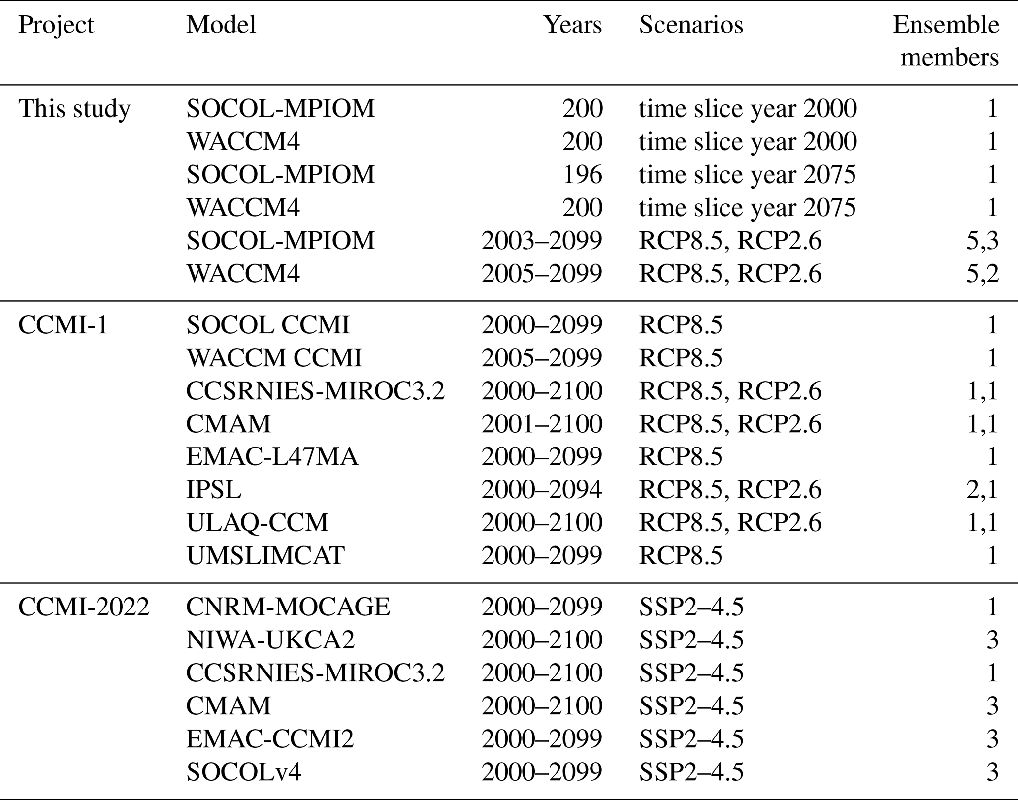
With the two CCMs, SOCOL-MPIOM (SOlar Climate Ozone Links coupled with the Max Planck Institute Ocean Model) and WACCM 3(Whole Atmosphere Community Climate Model) version 4, we perform both transient simulations of the 21st century for different emission scenarios and time slice simulations of the years 2000 and 2075. We further compare the results with corresponding simulations of the Chemistry-Climate Model Initiative (CCMI), CCMI-1 and CCMI-2022, as well as the reanalysis dataset MERRA2.
2.1 Chemistry–climate modelling
WACCM (the Whole Atmosphere Community Climate Model) is the atmospheric component of the NCAR Community Earth System Model version 1 (CESM1.2.2). WACCM has a horizontal resolution of 1.9∘ in latitude and 2.5∘ in longitude (Marsh et al., 2013) and is coupled to interactive ocean and sea ice components (Danabasoglu et al., 2012; Holland et al., 2012). Ozone concentrations are calculated interactively, including a total of 59 species (Marsh et al., 2013). With its well-resolved stratosphere and high model top ( hPa) on 66 vertical levels (Marsh et al., 2013), WACCM has been documented to capture stratospheric trends and variability reasonably well (Haase and Matthes, 2019; Rieder et al., 2019; Oehrlein et al., 2020).
SOCOL (SOlar Climate Ozone Links) version 3 is based on the middle atmosphere configuration of the general circulation model ECHAM5 (MA-ECHAM5), which is interactively coupled to the chemistry transport model MEZON (Model for Evaluation of oZONe trends Egorova et al., 2003). The model version SOCOL-MPIOM is additionally coupled to the ocean–sea-ice model MPIOM (Stenke et al., 2013; Muthers et al., 2014). SOCOL-MPIOM has a model top at 0.01 hPa, 39 vertical levels, and a horizontal resolution of 3.75∘ × 3.75∘ (Stenke et al., 2013). Ozone is calculated interactively based on a set of 140 gas-phase reactions, 46 photolysis reactions, and 16 heterogeneous reactions involving 41 species. Like WACCM, SOCOL-MPIOM captures stratospheric variability reasonably well (Muthers et al., 2014).
To gain an understanding of the dependency of stratospheric ozone trends and variability in the Arctic on the GHG loading, we compare simulations of high- and low-emission scenarios throughout the 21st century (2005–2099). For the high-emission scenario, GHGs follow the RCP8.5 pathway, whereas the low-emission scenario is based on the RCP2.6 pathway (Meinshausen et al., 2011); hODSs follow the A1 scenario according to WMO (2014). In addition to the transient simulations, we perform time slice simulations of the early (year 2000) and late (year 2075) 21st century with the fixed, seasonally varying GHGs and hODSs of the respective year. For simulations of the year 2075, boundary conditions follow the RCP8.5 pathway. In these time slice simulations, each covering 200 years, trends in stratospheric ozone and climate are omitted, allowing us to robustly assess long-term changes in the variability due to changes in GHG and hODS levels.
2.2 CCMI simulations
We compare our model results with sensitivity simulations of high-emission (SEN-C2-RCP85) and low-emission (SEN-C2-RCP26) scenarios conducted for phase 1 of CCMI (CCMI-1). GHG emissions of those simulations follow the RCP8.5 and RCP2.6 pathways (Meinshausen et al., 2011), respectively, with hODSs following the A1 scenario (WMO, 2011) . The high- and low-emission pathways therefore only differ in their assumptions regarding future GHG emissions, while hODSs are equal for both scenarios. Model simulations usually cover the period 2000–2100. We analyse all models that performed the SEN-C2-RCP85 simulation, namely SOCOL CCMI, WACCM CCMI, CCSRNIES-MIROC3.2, CMAM, EMAC-L47MA, IPSL, ULAQ-CCM, and UMSLIMCAT, with a subset of them also performing the SEN-C2-RCP26 simulation. The models participating in CCMI-1 exhibit substantial differences in the implementation of stratospheric (heterogeneous) chemistry and PSC schemes. For example, the amount of halogen source gases treated in the models varies between 2 (UMSLIMCAT) and 14 (SOCOL). For PSCs, some models assume thermodynamic equilibrium, while other models account for deviations from thermodynamic equilibrium. Further, some models explicitly include supercooled ternary solutions (STSs), and implementations differ in terms of PSC sedimentation across models. A detailed description of the CCMI-1 models is presented by Morgenstern et al. (2017).
To investigate the robustness of the evolution of ozone minima in CCMI models, we perform out-of-sample testing with CCMI-2022 simulations (SPARC, 2021). The moderate-emission scenario of CCMI-2022 simulations (REF-D2) follows the SSP2–4.5 pathway (Meinshausen et al., 2020), and hODSs follow the WMO (2018) baseline scenario. We analyse all models that performed the REF-D2 scenario, namely CNRM-MOCAGE, NIWA-UKCA2, CCSRNIES-MIROC3.2, CMAM, and EMAC-CCMI2. Model simulations were generally conducted for the time period 1960–2100. Here, we analyse the period 2000–2100. In addition to the CCMI-2022 simulations, we perform simulations with SOCOLv4 (Sukhodolov et al., 2021) following the CCMI-2022 REF-D2 boundary conditions. SOCOLv4 is an updated version of SOCOL-MPIOM based on the Earth system model MPI-ESM1.2 (Mauritsen et al., 2019), and it is additionally coupled to the sulfate aerosol microphysical model AER (Weisenstein et al., 1997). An overview of all model simulations and available ensemble members that were analysed in this study can be found in Table 1. For all models, we use the model output for Arctic mean ozone; temperature; and, where available, active chlorine species (ClOx = ClO + Cl + 2 Cl2O2) interpolated to pressure levels.
2.3 Reanalysis
Model results for the early 21st century are compared to the Modern-Era Retrospective Analysis for Research and Applications version 2 (MERRA2) for the period 1980–2020 (Gelaro et al., 2017). MERRA2 has a horizontal resolution of 0.5∘ × 0.625∘ and 72 vertical levels with a model top at 0.01 hPa, and we use 6-hourly instantaneous data output, which is then converted into monthly and springtime averages. MERRA2 has been shown to agree well with satellite and ozone sonde data regarding stratospheric ozone variability (Wargan et al., 2017; Davis et al., 2017; Bahramvash Shams et al., 2022). Further, we compare MERRA2 to the Stratospheric Water and Ozone Satellite Homogenized (SWOOSH) database for the period 2004–2020 using a horizontal resolution of 2.5∘ (Davis et al., 2016).
2.4 Analysis methods
Our analysis focuses on boreal spring, which we define as March–April averages, where ozone anomalies are maximized in the models. Unless stated otherwise, the results below show averages over the polar cap, defined as 60–90∘ N, applying latitudinal weighting according to the cosine of latitude. Lower-stratospheric ozone is defined as a partial ozone column between 30 and 70 hPa in DU (Friedel et al., 2022a). The ozone distributions shown contain all ensemble members of a simulation (without averaging). The mean magnitude of the ozone minima is defined as the lowest 20th percentile of springtime ozone anomalies for both time slice and transient (scenario) simulations. For time slice simulations, we thus average over the 40 lowest springtime ozone anomalies to derive the mean ozone minima strength. For transient simulations, we calculate the mean magnitude of ozone minima in a 25-year running window. For each window, the anomaly in each spring is calculated relative to the springtime climatology of that window, and the mean ozone minima are then calculated by averaging over the lowest 20th percentile of ozone anomalies (i.e. the 5 lowest springtime ozone values out of 25 springs). Uncertainty in the magnitude of the ozone minima is defined as the sensitivity to the inclusion of one more (6 out of 25) and one less (4 out of 25) spring into the calculation. For ensemble simulations with multiple members, this analysis is conducted for each ensemble member individually before averaging. Similarly, the temperature of particularly cold winters is defined as the lowest 20th percentile of springtime temperature at 50 hPa in a 25-year running window, and the uncertainty of this variable is calculated by including one more or one less spring in the calculation. For climatologies, uncertainties are given as standard deviations from the mean. For simulations containing multiple ensemble members, climatologies are calculated as ensemble means, and uncertainties are given as the root mean square of the individual members' uncertainties. Trends are generally estimated by linear least-squares regressions of the respective ensemble mean, and the uncertainty in trends is given by the standard error of the slope. The significance of trends is estimated by p values calculated using a Wald test (Fahrmeir et al., 2013).
3.1 Evolution of Arctic ozone minima in CCMI models
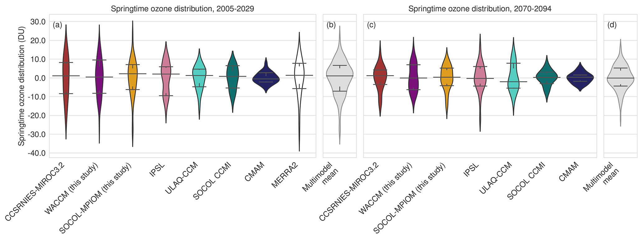
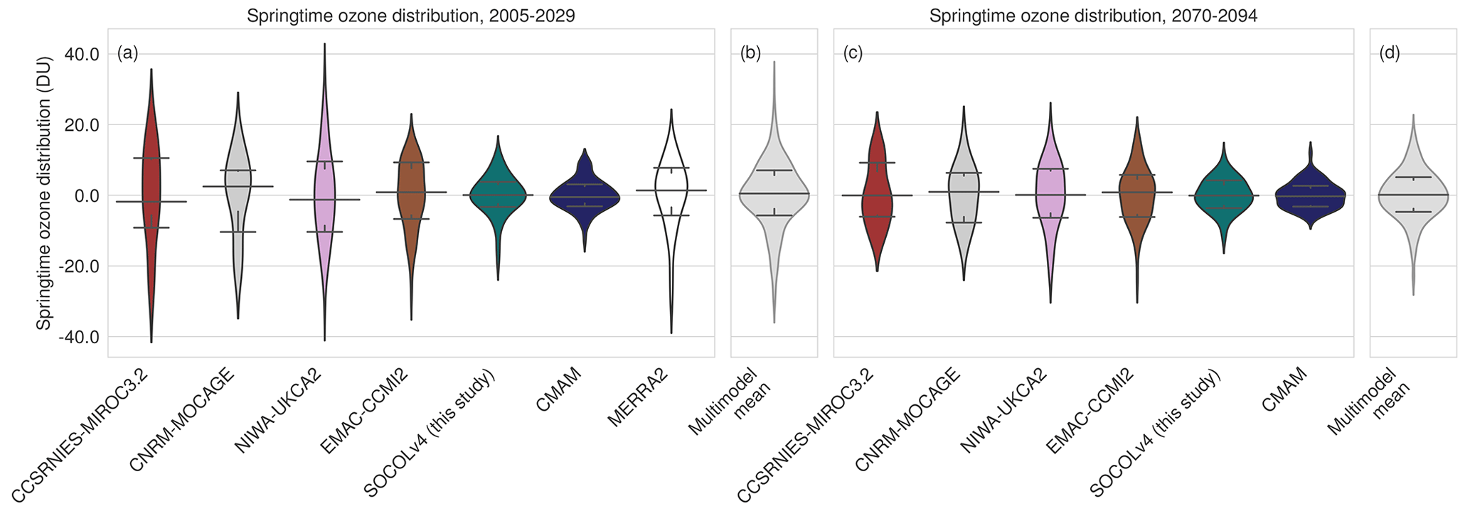
To identify the spread in simulated Arctic ozone and the evolution thereof across CCMs, we start by analysing springtime Arctic ozone anomalies in the early (2005–2029) and late (2070–2094) 21st century. Anomalies are defined as deviations from the climatology of the respective time period. Figure 1 shows distributions of Arctic lower-stratospheric ozone anomalies for the high-emissions scenario (RCP8.5) simulated with WACCM, SOCOL-MPIOM, and CCMI-1 models. In the following, we will concentrate on negative ozone anomalies. For the early time period (Fig. 1a), differences in the magnitude of ozone anomalies across models are striking; while some models simulate negative ozone anomalies larger than −40 DU for the springtime mean lower-stratospheric ozone column, other models barely show anomalies exceeding −5 DU. In the reanalysis product MERRA2, which covers recent-past to present-day climate (1980–2020), negative ozone anomalies reach up to −40 DU. Thus, most of the CCMs (7 out of 10) do not reproduce the most extreme negative ozone anomalies under current climatic conditions compared to reanalysis. In comparison, by the end of the century, CCMs provide a more coherent picture; almost all models simulate negative ozone anomalies, with a maximum of −20 DU. Thus, according to CCM simulations, extreme ozone loss beyond −20 DU is unlikely past 2070 in the high-emission scenario. Large ozone variability and extreme ozone loss comparable to MERRA2 is not projected by any model at the end of the century.
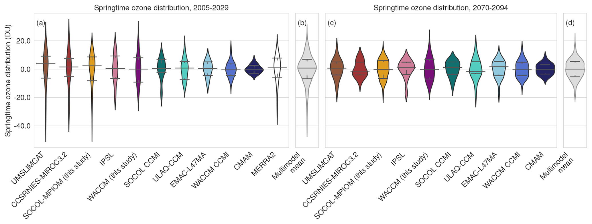
Figure 1Probability density distributions calculated based on kernel density estimation of stratospheric partial ozone column (30–70 hPa) in spring (March–April) normalized by the mean partial column ozone of the respective time period in the early (2005–2029 – a and b) and late (2070–2094 – c and d) 21st century in CCMI-1 models for RCP8.5. Whiskers show the 20th and 80th percentiles of the distributions. The multi-model mean shows the distributions over all models (excluding MERRA2) containing each ensemble member with equal weight. Similar figures for RCP2.6 and CCMI-2022 can be found in the Appendix (Figs. A2 and A3).
Further to changes in ozone anomalies, it is important to note that the mean ozone climatology is changing across the two time periods considered. Under the high-emission scenario, RCP8.5, Arctic stratospheric ozone is expected to increase from 136 to 153 DU in terms of the multimodel mean over the course of the 21st century (see Fig. A1) due to the combined impact of a range of processes: the decrease in hODSs, a strengthening of the Brewer–Dobson circulation (BDC) by GHGs (i.e. larger transport of ozone from the tropics to the poles) (Butchart, 2014), stratospheric cooling by GHGs in the tropical and mid-latitude regions (which slows down ozone depletion there), and increasing methane concentrations (Revell et al., 2012). This projection of an Arctic ozone recovery of 17 DU from 2000 until 2100 is consistent with what has been reported previously for the lower stratosphere in CCMI-1 models (Dhomse et al., 2018). The rise in mean ozone suggests that, even during the most severe projected negative anomalies of −20 DU by the end of the century, there will hardly be any less ozone than is the case with the current mean.
In the following, we will focus on the most extreme negative ozone anomalies, defined as the lower 20th percentile of springtime ozone anomalies and referred to as ozone minima. To examine changes in ozone minima over time, we calculate the ozone minima in a 25-year running window (i.e. average over the 5 most extreme negative ozone anomalies out of 25 springs). Ozone anomalies are thereby calculated with respect to the climatology in the corresponding window. Figure 2 shows the evolution of the ozone minima over time for all model simulations and different GHG emission pathways: RCP8.5 (Fig. 2a), RCP2.6 (Fig. 2c), and SSP2–4.5 (Fig. 2e). Again, there is a large scatter across the models in terms of the strength of the simulated ozone minima at the beginning of the century, ranging from −22.5 to −3 DU. Over time, the model spread decreases, and by the end of the century, it ranges from −10 and −3 DU. The uncertainty in the magnitude of ozone minima is therefore reduced over the course of the century. Models that simulate large ozone minima under current conditions (2005–2029) also show the largest ozone minima under future conditions (e.g. UMSLIMCAT), but the magnitude of these future minima is significantly smaller. In contrast, models with small ozone minima under present-day conditions (e.g. CMAM) show hardly any change in the magnitude of these minima under future conditions.
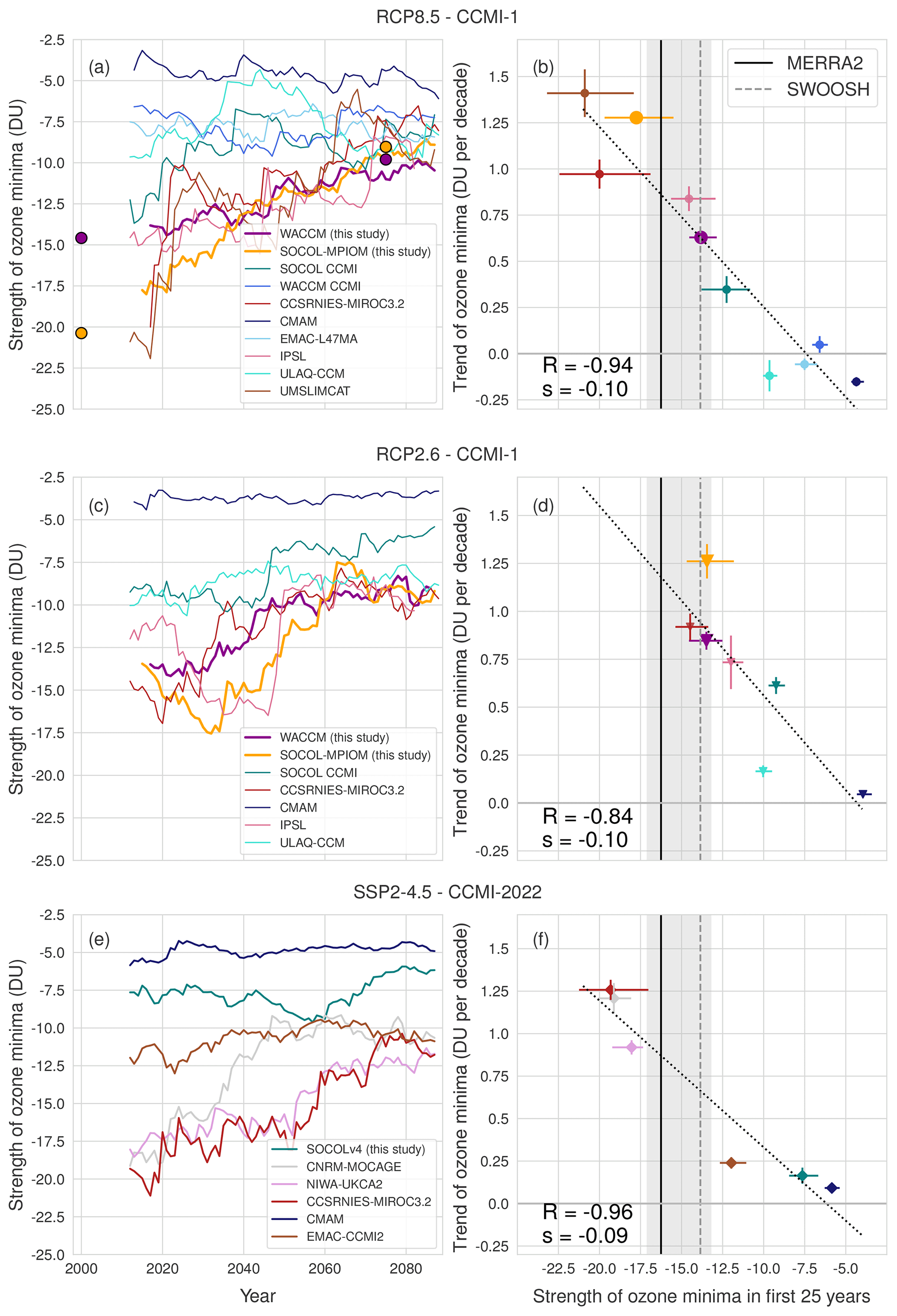
Figure 2Evolution of the strength of Arctic ozone minima in CCMI-1 models under RCP8.5 (a) and RCP2.6 (c), as well as for CCMI-2022 models under SSP2–4.5 (e). Correlation of the trend in ozone minima strength and the strength of the ozone minima in the first 25 years defined by the mean ozone anomaly of the 20th percentile (5 out of 25 strongest ozone minima in running window, normalized by the ozone climatology of running window) (b, d, f). The mean strength of ozone minima in MERRA2 from 1980 to 2020 is given by the solid black line. The grey shading shows the uncertainty of the MERRA2 ozone minima strength, as explained in the “Material and methods” section. The mean ozone minima strength in SWOOSH from 2004 to 2020 is shown by the stippled grey line. Circles in (a) show the ozone minima strength of the WACCM and SOCOL-MPIOM time slice simulations for the years 2000 and 2075, respectively.
The future decline in the magnitude of ozone minima is related to the magnitude of the Arctic ozone depletion under current conditions (see negative correlations of −0.84 to −0.96 in Fig. 2b, d, f). The development of ozone minima is thereby strongly correlated with the initial strength of the ozone minima in the respective model. Consequently, models with large ozone minima at the beginning of the century generally show larger trends towards less-pronounced ozone minima in the future, whereas models with small ozone minima show no trends at all. Linear regression of the trend in ozone minima to their initial magnitude shows that this relationship is independent of the emission scenario; i.e. the regression slope is the same across all scenarios considered (). The scenario independence suggests that greenhouse gases other than hODSs (such as carbon dioxide, methane, nitrous oxide, and water vapour), which differ among the scenarios, may not be critical to the development of ozone minima.
Given the strong correlation of the trend in ozone minima and their initial magnitude, the large inter-model spread can be used to constrain projections of future ozone minima by observations. To this end, we compare the simulated ozone minima in the present-day climate with ozone minima observed during the past 40 years (1980–2020) in MERRA2 (black line in Fig. 2 b, d, f) and find that the models that most realistically reproduce current ozone minima project a decrease in extreme negative ozone anomalies of about 1 DU per decade (see intersection of regression line and reanalysis). Hence, using past ozone minima in reanalyses as an emergent constraint suggests that extreme negative ozone anomalies will likely be 8–10 DU (and therefore around 50 %) less severe by the end of the 21st century. A similar result is found when using the SWOOSH database for the period 2004–2020 as an observational constraint, for which we define the ozone minima strength based on the three strongest ozone minima in that period (20th percentile – stippled grey line in Fig. 2b, d, f). It is to be noted that an emergent constraint analysis can only be a useful tool for reducing uncertainty in future projections if it (1) survives out-of-sample testing and (2) exhibits a physical mechanism underlying the strong statistical relationship (Hall et al., 2019; Simpson et al., 2021). While the former is fulfilled by the independence of the results from emission pathways and model sets, the latter will be discussed below.
A more precise method for estimating the likely evolution of ozone minima is weighted model means. Here, we calculate weights for each individual model based on their ability to reproduce the present-day ozone minima (performance) and their interdependence (i.e. the family relationship of some models) (Knutti et al., 2017; Amos et al., 2020; Morgenstern et al., 2017). The model weights are then used to calculate a weighted arithmetic mean of the trend in ozone minima. Resulting model weights and a more detailed description of the methodology can be found in the Appendix (Sect. A2). Weighted model means suggest a reduction of the magnitude of ozone minima of 1.0 (RCP8.5), 1.1 (RCP2.6), and 1.0 (SSP2–4.5) DU decade−1. Thus, weighted model means are largely scenario independent and agree well with estimates of the emergent-constraint approach.
Since many models only simulated one single ensemble member for future projections (see Table 1) and because the sample used for calculating the ozone minima is small (five springs per running window width), we test the sensitivity of our results to sample size using 200-year time slice simulations performed with the CCMs WACCM and SOCOL-MPIOM. By using fixed boundary conditions for the years 2000 and 2075, we omit any trends in ozone or temperature due to changes in hODSs and GHGs. Consistently with the previous definition, we again select the 20th percentile of the most extreme negative ozone anomalies (40 out of 200) to define the magnitude of the mean ozone minima in the time slice simulations. The ozone minima in these simulations, shown as circles in Fig. 2a, agree very well with the transient simulations, suggesting that the smaller sample size in transient simulations is sufficient to derive robust results (see also Fig. A6).
3.2 The source of model differences in the current climate
We have shown that model dispersion in simulated ozone can be useful in constraining the evolution of ozone minima. However, the question arises as to why CCMs show large differences in the magnitude of ozone minima under current climatic conditions in the first place. Arctic ozone minima are caused by both chemical ozone depletion and dynamical variability (Tegtmeier et al., 2008); usually, ozone minima are preceded by reduced wave activity and, consequently, a strengthening and cooling of the polar vortex, as well as a weakening of the BDC. Dynamical resupply of ozone to the polar region is therefore reduced, and cold temperatures allow for the formation of PSCs and chlorine activation, consequently leading to ozone depletion. The amount of ozone depleted thereby depends on the amount of active chlorine species (ClOx) in the stratosphere. In Fig. 3a, we show that the strength of ozone minima strongly correlates with the stratospheric Arctic mean ClOx concentrations (at 50 hPa) across models in the beginning of the 21st century. Hence, the differences in the magnitude of ozone minima in different models are attributable to differences in chemical ozone destruction by ClOx. The amount of activated chlorine in the stratosphere itself depends on the volume of the PSCs, which in turn is strongly temperature dependent. We find a large spread (around 10 K) in the mean Arctic stratospheric temperature across models in winter and spring (January–April). This model scatter is consistent with what has been reported previously by Morgenstern et al. (2022) for some CMIP6 and CCMI-2022 models. The reasons for such differences in the models' mean stratospheric springtime temperatures are likely linked to differences in the large-scale circulation, such as the BDC, or the lifetime and shape of the polar vortex. Here, we complement the analysis by Morgenstern et al. (2022) by connecting those temperature biases to ClOx concentrations and finally the magnitude of ozone minima. When linking the mean polar cap temperature at 50 hPa to stratospheric ClOx concentrations at the same altitude in the CCMs, we find a linear relationship, with a correlation coefficient of (see Fig. 3b). Thus, differences in ClOx concentrations among models can largely be attributed to temperature biases. Models which show a warm temperature bias (e.g. CMAM – dark-blue markers) under present-day conditions compared to MERRA2 (vertical solid black line in Fig. 3b) generally have small ClOx concentrations (Fig. 3a) and thus simulate only weak ozone depletion and consequently weak Arctic ozone minima. In turn, models with a cold-temperature bias (e.g. CCSRNIES-MIROC3.2 – red markers) simulate large ClOx concentrations, strong ozone depletion, and large ozone minima. Models which best reproduce the Arctic mean temperature from MERRA2 generally also agree better with MERRA2 in terms of the magnitude of the simulated Arctic ozone minima. This behaviour compares well with previous results showing that temperature biases limit the models' ability to reproduce observed PSC coverage (Snels et al., 2019; Steiner et al., 2021).
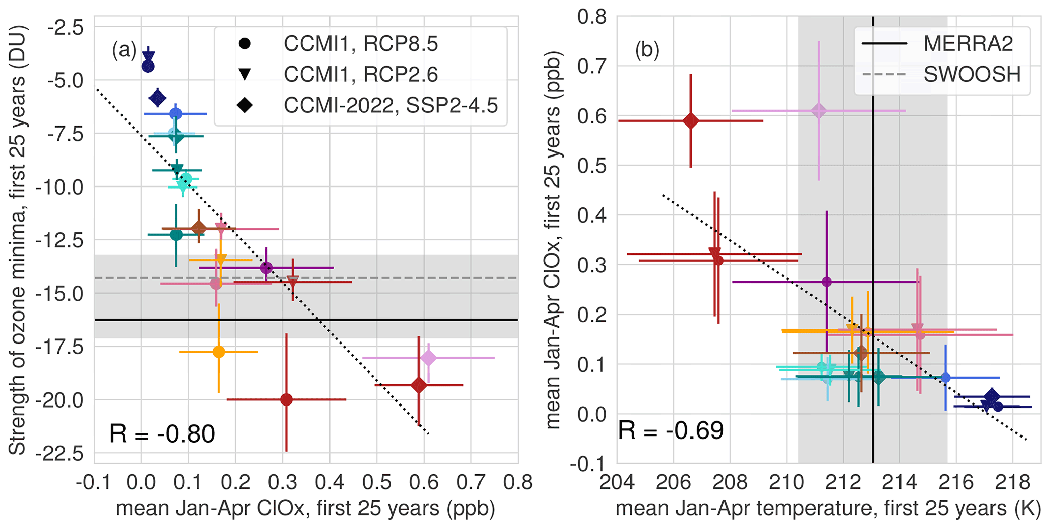
Figure 3Relation between ClOx concentration in late winter and spring (January–April) at 50 hPa and the strength of the ozone minima in the first 25 years (a), as well as the relation between ClOx concentrations and mean temperature in January–April in the first 25 years of simulation (b). Colours indicate the different models as in Figs. 1 and 2. The dotted black lines show the linear regression. The Pearson correlation coefficient is denoted by R. The mean ozone minima strength and the mean temperature in MERRA2 are shown by the black lines. The shading and vertical error bars in (a) show the uncertainty of ozone minima strength, as explained in the methods section. The mean ozone minima strength in SWOOSH from 2004–2020 is shown by the stippled grey line in (a). Grey shading, as well as error bars in (b), shows the standard deviation.
Besides temperature biases, differences in total inorganic chlorine (Cly) across models could partly be responsible for model differences in ClOx. A large inter-model spread in Cly in CCM simulations has been reported previously by Eyring et al. (2006, 2007) and has been attributed to differences in the transport of chemical species within the stratosphere (Eyring et al., 2006). Moreover, differences in the number of chlorine source gases considered (Morgenstern et al., 2017) and in the overall treatment of photolysis in the models (Sukhodolov et al., 2016) could contribute to the biases in the ozone minima. However, for the Arctic region, the correlation between Cly and ClOx concentrations is low across the models analysed here (see Fig. A7 in the Appendix).
3.3 The source of model differences in future projections
Now that we have established the reasons for differences in simulated ozone minima in the current climate across models, we investigate the reasons for the differences in future ozone minima trends. Trends in ozone loss are impacted by both the decline in hODS concentrations and the potential changes in stratospheric temperature due to GHG emissions, which might impact the formation of PSCs. In addition, dynamical changes might contribute to temperature trends, as discussed below. Besides, an increase in stratospheric water vapour might change the abundance of PSCs in the future (von der Gathen et al., 2021). In Fig. 4, we investigate both the relationship of declining ClOx and the temperature trends with changes in ozone minima. Trends in ozone minima are strongly correlated with changes in ClOx concentrations; models with large ClOx concentrations under the current climate (e.g. CCSRNIES-MIROC3.2 – red markers) show a large decline in ClOx over the next century and therefore a large decline in ozone loss. Models that have low ClOx concentrations to start with (e.g. CMAM – dark-blue markers) show almost no changes in active chlorine species in the future and thus barely any changes in ozone loss. The development of ozone minima in individual CCMs is therefore strongly driven by changes in stratospheric ClOx concentrations.
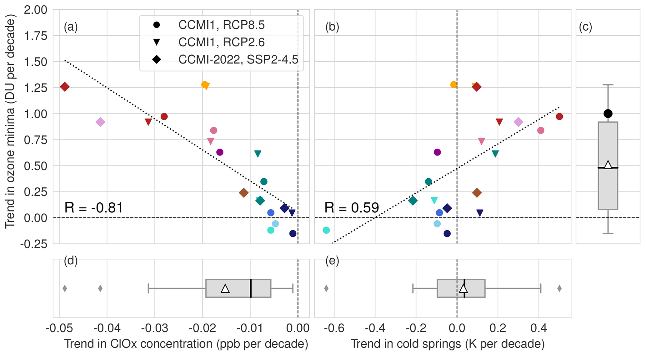
Figure 4Dependence of the trend in ozone minima on the trend in ClOx concentrations (a) and on the 50 hPa temperature trend in cold springs (b). Colours indicate the different models as in Figs. 1 and 2. A positive trend in ozone minima strength means a decrease in the magnitude of ozone minima in the future. Negative temperature trends mean that cold winters and springs are getting colder, and positive temperature trends mean that cold winters and springs will be less extreme in the future. Dotted black lines show the linear regression. The Pearson correlation coefficient is denoted by R. Box plots show changes in the mean ozone minima strength (c), ClOx changes (d), and temperature changes in cold springs (e) across models and scenarios. Triangles mark the median change, and black lines mark the mean change across models. The circle in (c) shows the weighted arithmetic model mean. Note that not all models used to calculate the weighted mean are shown in (a) and (b) due to lack of ClOx data in some models.
Next, we investigate the relation between long-term changes in Arctic stratospheric temperature and ozone minima. For ozone minima, the temperature evolution of the coldest winters and springs is most relevant as large amounts of PSCs and severe ozone loss are expected only under sufficiently cold conditions (< 196 K). Further, it has previously been shown that GHG cooling especially impacts the PSC formation in extremely cold Arctic winters (Rex et al., 2004; Tilmes et al., 2006; von der Gathen et al., 2021). We therefore focus on the temperature evolution of the coldest 20 % of the winter and spring seasons (January–April mean) in a 25-year running window, similarly to Morgenstern et al. (2022). Overall, CCMs do not agree on the sign of stratospheric temperature trends in late winter and spring in especially cold years (Fig. 4b). In addition, models also do not agree on the temperature response to additional GHG forcing (see temperature trends for RCP2.6 vs. RCP8.5 in the individual models). On average, models show a slightly positive temperature trend (consistent with the weak but significant Arctic warming projected in boreal spring reported in the WMO (2018) assessment; see their Figs. 5–8), but the spread ranges from −0.6 to +0.5 K decade−1 (Fig. 4e). This inter-model spread is consistent with what has been reported previously for CCMVal2 models (Bohlinger et al., 2014). Overall, the correlation between stratospheric temperature trends and changes in ozone minima is moderate (0.59) and is mainly caused by the two most extreme negative (ULAQ-CCM) and positive (CCSRNIES-MIROC3.2) values. For the bulk of the models that show no or only minor temperature changes (within −0.2 and 0.2 K decade−1), the temperature trends do not seem to be connected with trends in ozone minima (Fig. 4b). Thus, for this majority of models, different trends in ClOx concentrations drive different trends in ozone minima, and temperature changes only play a secondary role. However, for models with large temperature trends, like ULAQ-CCM (−0.6 K decade−1) and CCSRNIES-MIROC3.2 (+0.5 K decade−1), changes in temperature seem to be reflected in ozone minima trends. For example, in the extreme example of ULAQ-CCM, cold winter and spring seasons become extensively colder in the future (see round turquoise marker in Fig. 3b), which results in a more efficient activation of ClOx. The more efficient activation of ClOx is in opposition to the decline in atmospheric CFC concentrations. As a result, the ClOx concentration and the magnitude of ozone minima hardly change in this model (see Figs. 1 and 2b).
To highlight the uncertainty in Arctic stratospheric temperature trends in CCMs, we show temperature trends in extremely cold boreal winters (January–April mean) for the whole atmosphere for the high-emission scenario RCP8.5 in Fig. 5. Although the models agree on the sign of the temperature changes in the troposphere and most of the stratosphere, there are large inter-model differences for the Arctic lower stratosphere (marked by the grey square), with some models projecting a warming and others projecting cooling. This uncertainty is most likely due to several competing processes that contribute to stratospheric temperature trends over the Arctic; GHGs radiatively cool the stratosphere. This GHG cooling is responsible for the negative temperature trends in large parts of the stratosphere. At the same time, the forthcoming recovery of Arctic ozone (see Fig. A1) is expected to radiatively heat the stratosphere, offsetting a great part of the GHG cooling (Maycock, 2016; Kult-Herdin et al., 2023). In addition to changes in radiation, changes in large-scale dynamics are expected to impact stratospheric temperature. In particular, a projected strengthening of the Brewer–Dobson circulation (BDC) due to increasing GHGs will drive a stronger downwelling and associated adiabatic dynamical heating over the North Pole (Butchart, 2014). Since CCMs show different sensitivities to GHG and hODS forcings (Morgenstern et al., 2018), the contribution of the individual processes to temperature trends might vary across models. For example, the evolution of stratospheric dynamics and dynamical variability in the Arctic is very uncertain and highly model dependent (Ayarzagüena et al., 2018, 2020; Abalos et al., 2021; Karpechko et al., 2022), which likely contributes to the uncertainty in Arctic stratospheric temperature trends. In this context, it has already been shown that both radiative and dynamical processes add to the projected temperature spread across CCMs in the lower stratosphere (Bohlinger et al., 2014).
In summary, changes in the magnitude of ozone minima are strongly correlated to the decrease in ClOx across models. Changes in the temperature of cold winters, however, only correlate with changes in ozone minima in models with extreme temperature trends ( K decade−1). Thus, we conclude that long-term changes in Arctic ozone minima are strongly driven by long-term changes in stratospheric ClOx concentrations. Changes in temperature, on the other hand, seem to play a secondary role in the evolution of Arctic ozone minima for the majority of the models. The relation between changes in ClOx and changes in ozone minima serves as an underlying physical mechanism for the emergent constraint analysis, as described above. Even if temperature trends are not decisive for the development of ozone minima, it should again be emphasized that temperature biases in the mean state are important to explain the large model scatter in the magnitude of ozone minima under present-day conditions.
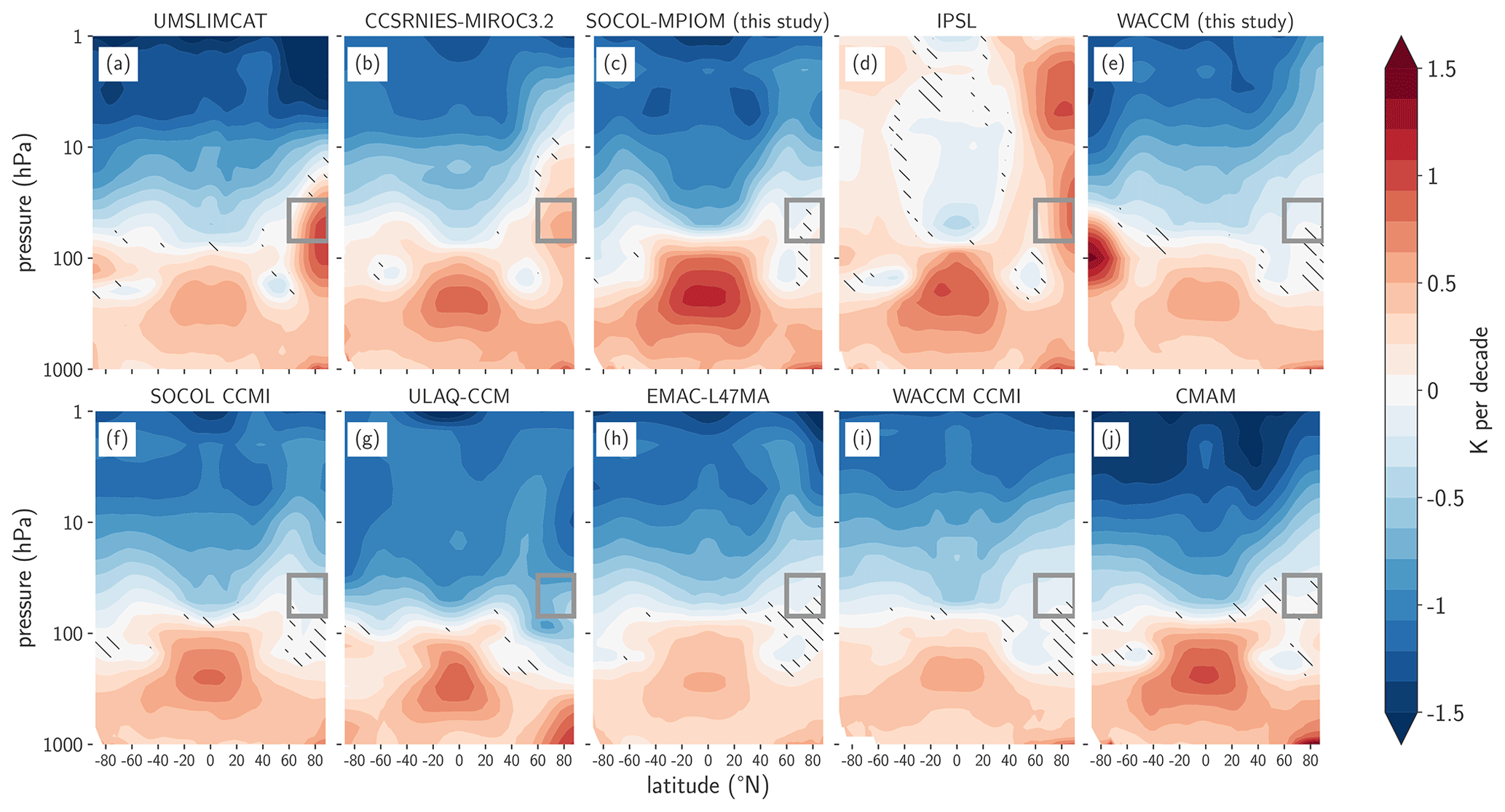
Figure 5Temperature trend of the coldest 20 % of the winter and spring seasons (January–April mean) in a 25-year running window over the course of the 21st century in CCMI1 models for RCP8.5. Stippling marks regions which are not significant at the 5 % level. The grey square marks the region of interest (60–90∘ N polar cap, 30–70 hPa).
Previous studies reported a large spread in Arctic ozone minima across CCMs and questioned the reliability of simulated ozone (von der Gathen et al., 2023; Morgenstern et al., 2018). Therefore, past studies derived trends in ozone loss from trends in temperature and PSC formation potential rather than trends in ozone itself (Rex et al., 2004; Rieder and Polvani, 2013; Langematz et al., 2014; von der Gathen et al., 2021). This study sheds new light on the origin of these model differences and shows how they can be useful in constraining future projections. Here, we show that differences in the magnitude of ozone minima across models under current conditions are largely due to temperature biases, which lead to different amounts of active chlorine species in the Arctic polar stratosphere. The amount of stratospheric ClOx in the Arctic and thus the magnitude of the ozone minima at the beginning of the 21st century thereby determine the future trend of negative ozone anomalies: models with high chlorine activation and large ozone minima show a large trend towards less-pronounced ozone minima in the future, while models with little chlorine activation and small ozone minima hardly show any trends. Therefore, the uncertainty in the magnitude of ozone minima will decrease in the future, leading to a better agreement of future ozone minima in CCMs. Moreover, the spread across CCMs can be an advantage in constraining the evolution of ozone minima as the initial strength of the ozone minima is strongly correlated with its trend. An emergent constraint approach estimates a decline in the magnitude of Arctic ozone minima of about −1 DU decade−1, and model simulations suggest that the most severe Arctic ozone anomalies are unlikely to surpass −20 DU by the end of this century. Drastic ozone depletion events, like the one observed in spring 2020 (Lawrence et al., 2020), will thus become very unlikely by the end of this century. A similar result can be gained when weighting the model projections according to their performance and interdependence. Such a weighted model average again suggests a decline in the magnitude of Arctic ozone minima of −1 DU decade−1, independent of the GHG scenario. This result is in line with findings reported by Polvani et al. (2023), which show that the absolute value of ensemble minimum Arctic ozone consistently increases in CMIP6 models that employ interactive ozone chemistry.
The absence of extreme Arctic ozone minima past 2070 in the CCMs analysed here stands in an apparent contrast to results reported by von der Gathen et al. (2021), who suggest that large Arctic ozone loss might still be possible or may even increase by the end of the 21st century under high-GHG-emission scenarios. However, there are substantial differences in the methods and variables used in the two studies. First, von der Gathen et al. (2021) infer chemical ozone loss inside the polar vortex area from temperature trends in CMIP6 models, whereas, here, we analyse the actual ozone output averaged over the polar cap from CCMs. As such, the ozone minima analysed here are the result of both chemical ozone loss and changes in ozone transport and thus represent the full extent of the ozone anomaly instead of just the chemical contribution. Second, differences in the results might arise from the different time periods considered: while the results presented here focus on average seasonal springtime ozone (March–April), von der Gathen et al. (2021) focus on changes in PSC formation potential over the whole winter-to-spring period at a daily resolution. In addition, von der Gathen et al. (2021) adjust the calculated ozone loss according to estimated changes in stratospheric water vapour, while in the CCMs presented here, such changes are calculated interactively in the models. Taken together, the results presented here are not necessarily inconsistent with results from von der Gathen et al. (2021) but rather complement their study by considering the full extent of negative ozone anomalies over the whole season rather than only the short-term chemical ozone loss. Similarly, the decrease in Arctic ozone minima as suggested by CCMI models seems to contradict results from Bednarz et al. (2016) and Akiyoshi et al. (2023), who found that large ozone minima past 2060 might be still be possible in their models (UM-UKCA and MIROC3.2), although rarely. The versions of these models (NIWA-UKCA2 and CCSRNIES-MIROC3.2) analysed here are both outliers in terms of present-day polar ClOx concentrations (see Fig. 3a, pink and red diamonds), which cannot be explained by the models' temperatures (see Fig. 3b). In these models, there is still a comparably large amount of ClOx available at the end of the 21st century. While these conditions might be responsible for the episodic ozone minima past 2060 reported by Bednarz et al. (2016) and Akiyoshi et al. (2023), there is no sign of worsening of ozone minima in the future in these models. Rather, the two models consistently indicate a decreasing magnitude of ozone minima over time.
Ozone minima have previously been reported to influence Northern Hemispheric spring climate via their impact on stratospheric temperature and dynamics (Friedel et al., 2022a, b). With the reduction of such ozone minima in future climates, their ability to influence stratospheric temperatures may diminish, and consequently, their role as a driver of springtime surface climate may become less important. However, there is no consensus on the development of stratosphere–troposphere coupling in the future, and further investigation is necessary to draw conclusions about the relevance of future Arctic ozone minima for tropospheric climate. Due to the changes in the Arctic mean ozone levels, extreme Arctic ozone minima in the future will hardly surpass the mean ozone levels of today. Health-related impacts of ozone minima (due to the impacts on UV exposure) are therefore likely to decrease. It is to be noted, though, that the results presented here are based on seasonal averages, which might mask processes (on the basis of days to weeks) that are potentially important for health and climate. In addition, there are other Earth system processes that are not captured by the CCMs considered here, e.g. wildfires, which might affect the future evolution of Arctic ozone minima.
As negative ozone anomalies decrease, so does interannual ozone variability (see Fig. 1). Under current conditions, ozone variability is an important driver of Arctic stratospheric temperature and dynamical variability in CCMs (Rieder et al., 2019; Friedel et al., 2022b), and interactive ozone chemistry is considered to be important for a realistic representation of the stratosphere. Moreover, the statistical connection between stratospheric ozone anomalies and surface climate suggests that accounting for interactive ozone chemistry in forecast models could provide a potential source of predictability on subseasonal to seasonal scales. Whether this relationship and the potential importance of interactive ozone for predictability will hold in the future will require further investigation. However, since not only ozone minima but also positive ozone anomalies have been shown to significantly impact surface climate in spring (Friedel et al., 2022b), ozone variability can be expected to continue playing a role for both stratospheric and surface climate in the future.
A1 Ozone distributions
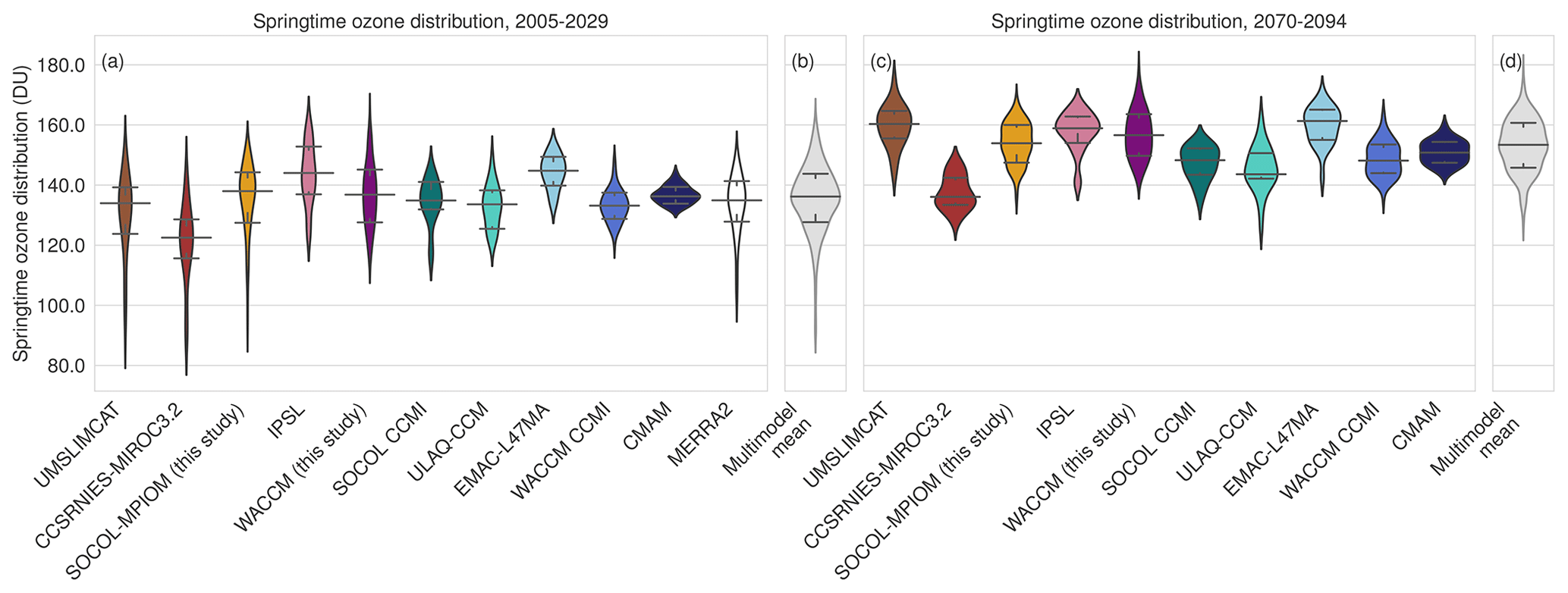
Figure A1Same as Fig. 1 but with absolute ozone values instead of ozone anomalies. As such, the change in distributions between the early (a) and late (b) 21st century conveys both changes in ozone extremes (see lower tail of the distributions) and the ozone recovery, which is reflected in changes of the climatology.
A2 Calculation of the weighted model mean
A weighted model average is calculated to estimate the trend in the magnitude of Arctic ozone minima, similarly to the method used by Knutti et al. (2017) and Amos et al. (2020). Model weights are calculated based on their ability to represent the magnitude of ozone minima under present-day conditions. Given N models, the weight wi of model i is calculated according to
where Di is the difference between the simulated and observed magnitude of ozone minima, and Sij is the difference between models i and j. σD and σS are both assumed to be 0.01, as in Amos et al. (2020). Weights are then normalized so that their sum is equal to 1 (Knutti et al., 2017). The weights calculated following this method are shown in Fig. A4. A weighted arithmetic mean of the trajectories for the ozone minima strength is then calculated for each scenario independently (see Fig. A5), and trends of the mean trajectories are calculated. The trends derived in this way are 1.0 (RCP8.5), 1.1 (RCP2.6), and 1.0 (SSP2–4.5) DU decade−1.
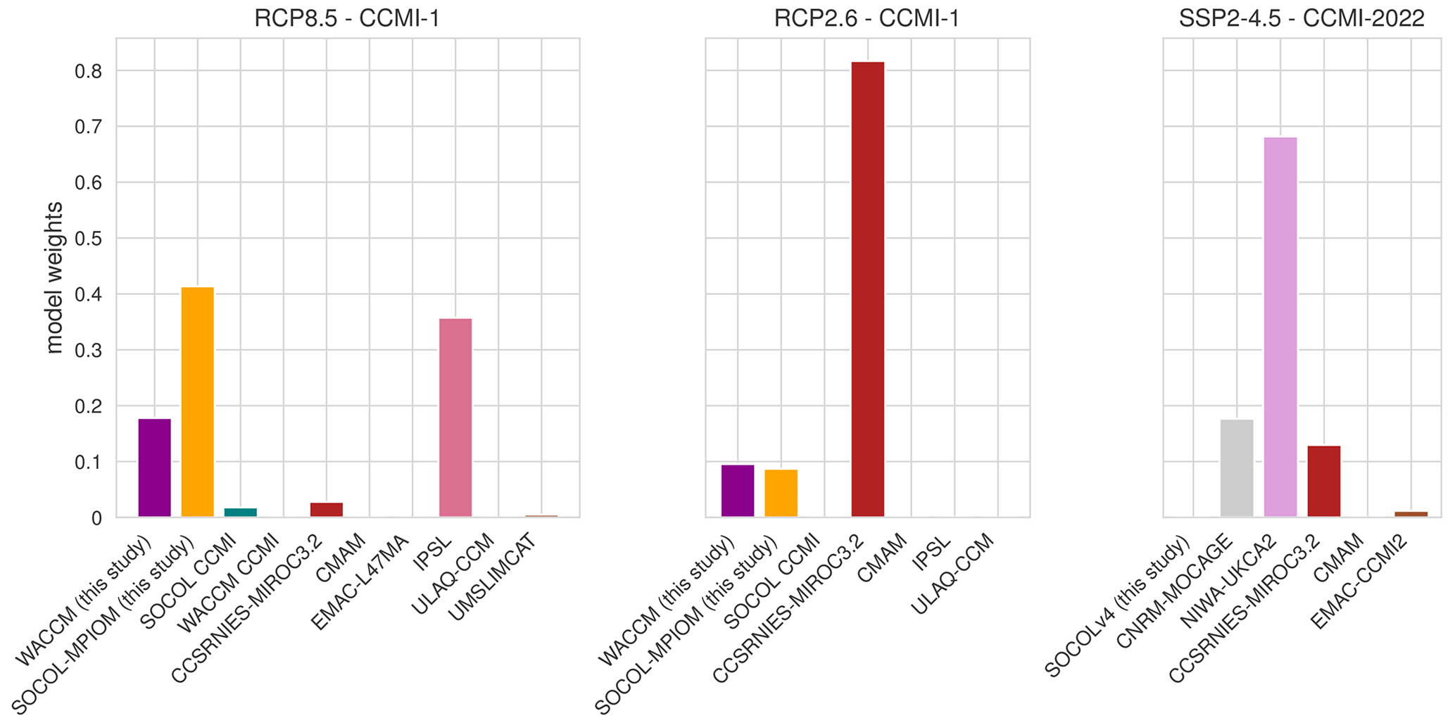
Figure A4Model weights calculated based on the model's ability to reproduce observed ozone minima and interdependence.
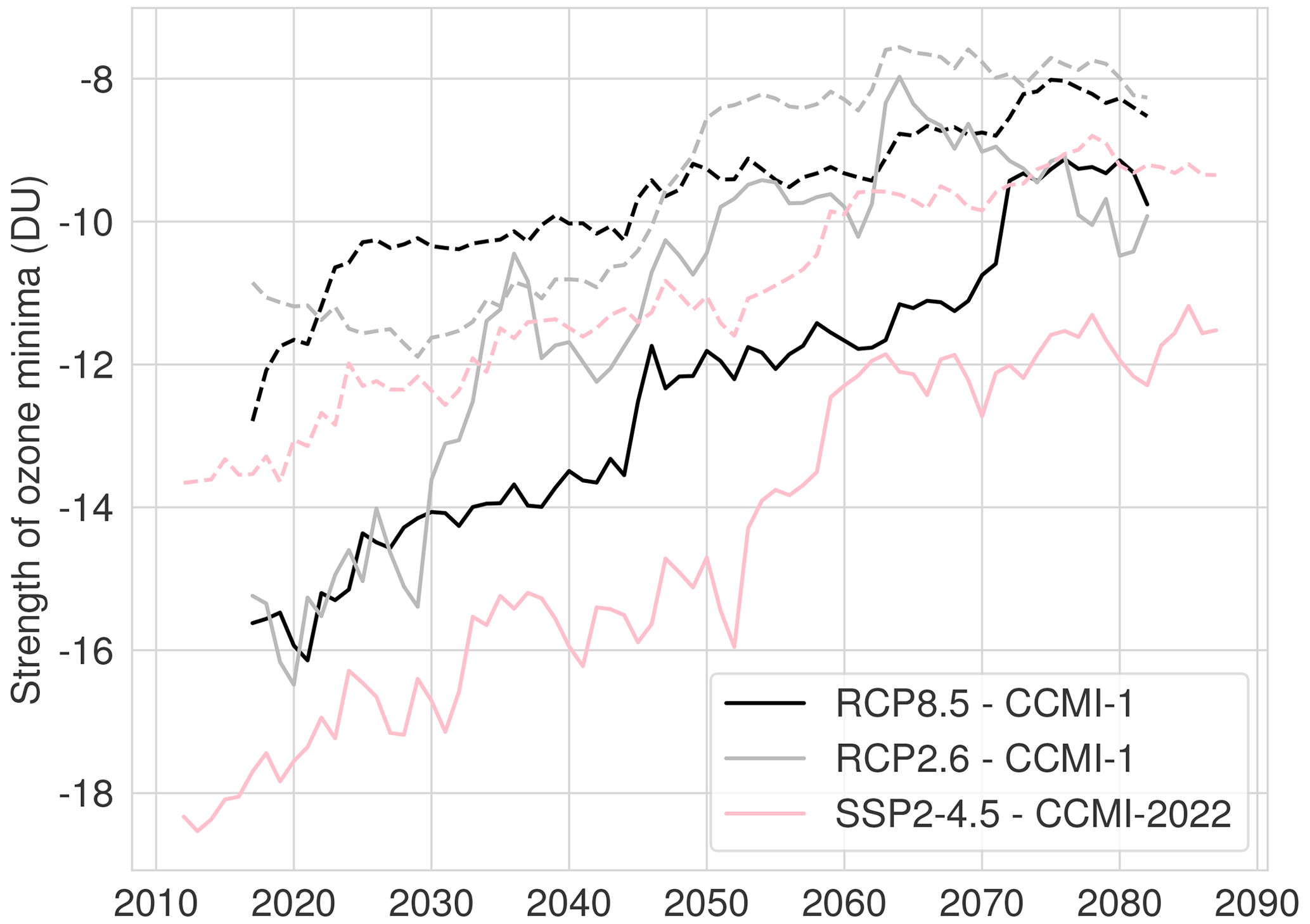
Figure A5The weighted arithmetic mean (solid lines) and unweighted multi-model mean (stippled lines) for the evolution of the ozone minima strength in the three scenarios considered.
A3 Time slice simulations
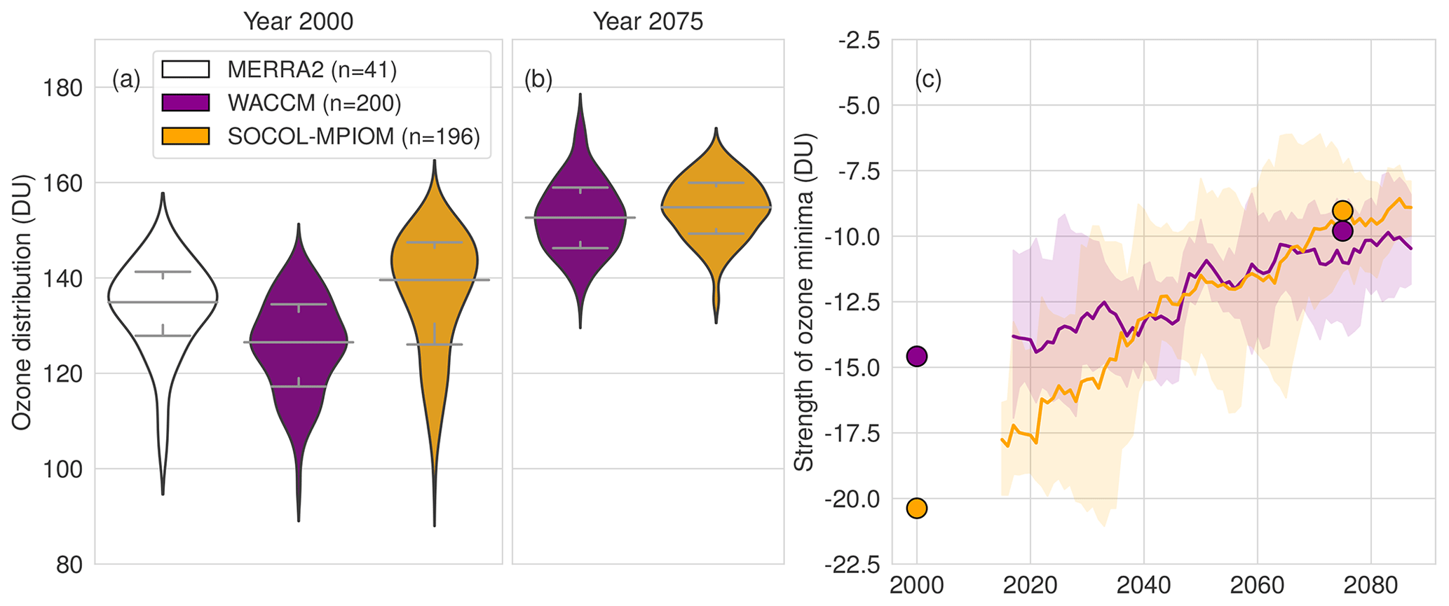
Figure A6Mean distribution of springtime Arctic ozone in time slice simulations of the year 2000 for SOCOL-MPIOM and WACCM, as well as MERRA2 mean springtime ozone distribution from 1980 to 2020 (a). Mean distribution of springtime Arctic ozone in time slice simulations of the year 2075 for SOCOL-MPIOM and WACCM (b). Development of the strength of ozone minima in WACCM and SOCOL-MPIOM RCP8.5 simulations (solid lines), as well as the mean strength of the strongest 20 % of ozone minima in the time slice simulations for the years 2000 and 2075 (circles). Shading shows the maximum and minimum values across the five ensemble members.
A4 Relation of Cly and ClOx in CCMI-1 RCP8.5
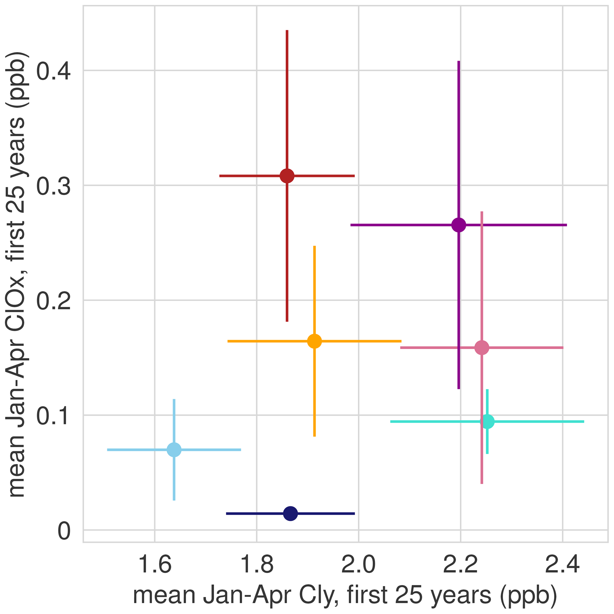
Figure A7Relation of Cly and ClOx concentration (2005–2029 climatologies) in late winter and spring (January–April) at 50 hPa for CCMI-1 models under RCP8.5. Colours indicate the different models, as in Fig. A1. The small vertical whisker for CMAM (dark blue) is hidden by the marker and results from the small interannual variability and thus the small uncertainty in ClOx.
The CCMI-1 and CCMI-2022 data used in this study can be obtained through the British Atmospheric Data Centre (BADC) archive (http://data.ceda.ac.uk/badc/wcrp-ccmi/data/CCMI-1/output/ (last access: 23 November 2022, CEDA Archive) and https://data.ceda.ac.uk/badc/ccmi/data/post-cmip6/ccmi-2022 (last access: 24 November 2022, CEDA Archive). The present-day time slice simulations used in this study are available in the ETH Research Collection. Data for WACCM can be found at https://doi.org/10.3929/ethz-b-000527155 (Friedel and Chiodo, 2022b). Data for SOCOL-MPIOM can be found at https://doi.org/10.3929/ethz-b-000546039 (Friedel and Chiodo, 2022a). All scripts used for the analysis in this study are available upon request. The MERRA2 reanalysis data can be downloaded from the Goddard Earth Sciences Data and Information Services Center (GES DIC) (https://doi.org/10.5067/VJAFPLI1CSIV, GMAO, 2015). The SWOOSH ozone dataset can be downloaded using the following link: https://csl.noaa.gov/groups/csl8/swoosh/ (Davis et al., 2016). Data for WACCM and SOCOL-MPIOM RCP8.5 simulations are found at https://doi.org/10.3929/ethz-b-000627740 (Friedel et al., 2023a). The WACCM and SOCOL-MPIOM time-slice simulations for the year 2075 can be found at https://doi.org/10.3929/ethz-b-000627743 (Friedel et al., 2023b).
MF, GC, TS, AS, and SvS performed and processed the SOCOL and WACCM experiments. HA, ER, DP, PJ, GZ, OM, and BJ performed and processed the CCMI experiments. MF analysed the results, and MF, GC, TP, and JK interpreted the results. MF wrote the paper with input from all the co-authors.
At least one of the (co-)authors is a member of the editorial board of Atmospheric Chemistry and Physics. The peer-review process was guided by an independent editor, and the authors also have no other competing interests to declare.
Publisher’s note: Copernicus Publications remains neutral with regard to jurisdictional claims in published maps and institutional affiliations.
We acknowledge the modelling groups for making their simulations available for this analysis, the joint WCRP SPARC/IGAC Chemistry-Climate Model Initiative (CCMI) for organizing and coordinating the model data analysis activity, and the Centre for Environmental Data Analysis (CEDA) for collecting and archiving the CCMI model output. Support from the Swiss National Science Foundation through the Ambizione Grant (grant no. PZ00P2_180043) for Marina Friedel and Gabriel Chiodo is gratefully acknowledged. The EMAC model simulations were performed at the German Climate Computing Centre (DKRZ) with support from the Bundesministerium für Bildung und Forschung (BMBF). DKRZ and its scientific-steering committee are gratefully acknowledged for providing the HPC and data-archiving resources for the consortial project ESCiMo (Earth System Chemistry integrated Modelling). James Keeble would like to thank the Met Office CSSP-China Programme for providing funding support through the POzSUM project and NERC for the funding support through the InHALE project. Hideharu Akiyoshi acknowledges the Environment Research and Technology Development Fund of the Environmental Restoration and Conservation Agency, Japan (grant nos. 2-1303 and JPMEERF20172009); KAKENHI (grant nos. JP18KK0289 and JP20H01977) of the Ministry of Education, Culture, Sports, Science, and Technology, Japan; and NEC SX-ACE and SX-AURORA TSUBASA computers at NIES. The authors wish to acknowledge the use of the New Zealand eScience Infrastructure (NeSI) high-performance computing facilities, as well as the consulting support and/or training services as part of this research. New Zealand's national facilities were provided by NeSI and funded jointly by NeSI's collaborator institutions and through the Ministry of Business, Innovation and Employment's Research Infrastructure programme (https://www.nesi.org.nz). Guang Zeng and Olaf Morgenstern acknowledge funding by the New Zealand Ministry of Business, Innovation and Employment (MBIE) under their Strategic Science Investment Fund (SSIF). Eugene Rozanov and Timofei Sukhodolov acknowledge support from the Swiss National Science Foundation (grant no. 200020-182239). Calculations with the SOCOLv4 were performed at the Swiss National Supercomputing Centre (CSCS) under project nos. S-901 (ID 154), S-1029 (ID 249), and S-903. The authors also thank Sean Davis (NOAA) for providing the SWOOSH data.
This research has been supported by the Schweizerischer Nationalfonds zur Förderung der Wissenschaftlichen Forschung (grant nos. PZ00P2_180043 and 200020-182239); the Environmental Restoration and Conservation Agency (grant nos. 2-1303 and JPMEERF20172009); the Ministry of Education, Culture, Sports, Science and Technology (grant nos. JP18KK0289 and JP20H01977).
This paper was edited by Simone Tilmes and reviewed by two anonymous referees.
Abalos, M., Calvo, N., Benito-Barca, S., Garny, H., Hardiman, S. C., Lin, P., Andrews, M. B., Butchart, N., Garcia, R., Orbe, C., Saint-Martin, D., Watanabe, S., and Yoshida, K.: The Brewer–Dobson circulation in CMIP6, Atmos. Chem. Phys., 21, 13571–13591, https://doi.org/10.5194/acp-21-13571-2021, 2021. a
Akiyoshi, H., Kadowaki, M., Yamashita, Y., and Nagatomo, T.: Dependence of column ozone on future ODSs and GHGs in the variability of 500-ensemble members, Sci. Rep.-UK, 13, 320, https://doi.org/10.1038/s41598-023-27635-y, 2023. a, b, c
Amos, M., Young, P. J., Hosking, J. S., Lamarque, J.-F., Abraham, N. L., Akiyoshi, H., Archibald, A. T., Bekki, S., Deushi, M., Jöckel, P., Kinnison, D., Kirner, O., Kunze, M., Marchand, M., Plummer, D. A., Saint-Martin, D., Sudo, K., Tilmes, S., and Yamashita, Y.: Projecting ozone hole recovery using an ensemble of chemistry–climate models weighted by model performance and independence, Atmos. Chem. Phys., 20, 9961–9977, https://doi.org/10.5194/acp-20-9961-2020, 2020. a, b, c, d
Ayarzagüena, B., Polvani, L. M., Langematz, U., Akiyoshi, H., Bekki, S., Butchart, N., Dameris, M., Deushi, M., Hardiman, S. C., Jöckel, P., Klekociuk, A., Marchand, M., Michou, M., Morgenstern, O., O'Connor, F. M., Oman, L. D., Plummer, D. A., Revell, L., Rozanov, E., Saint-Martin, D., Scinocca, J., Stenke, A., Stone, K., Yamashita, Y., Yoshida, K., and Zeng, G.: No robust evidence of future changes in major stratospheric sudden warmings: a multi-model assessment from CCMI, Atmos. Chem. Phys., 18, 11277–11287, https://doi.org/10.5194/acp-18-11277-2018, 2018. a
Ayarzagüena, B., Charlton-Perez, A. J., Butler, A. H., Hitchcock, P., Simpson, I. R., Polvani, L. M., Butchart, N., Gerber, E. P., Gray, L., Hassler, B., Lin, P., Lott, F., Manzini, E., Mizuta, R., Orbe, C., Osprey, S., Saint-Martin, D., Sigmond, M., Taguchi, M., Volodin, E. M., and Watanabe, S.: Uncertainty in the Response of Sudden Stratospheric Warmings and Stratosphere-Troposphere Coupling to Quadrupled CO2 Concentrations in CMIP6 Models, J. Geophys. Res.-Atmos., 125, e2019JD032345, https://doi.org/10.1029/2019JD032345, 2020. a
Bahramvash Shams, S., Walden, V. P., Hannigan, J. W., Randel, W. J., Petropavlovskikh, I. V., Butler, A. H., and de la Cámara, A.: Analyzing ozone variations and uncertainties at high latitudes during sudden stratospheric warming events using MERRA-2, Atmos. Chem. Phys., 22, 5435–5458, https://doi.org/10.5194/acp-22-5435-2022, 2022. a
Bednarz, E. M., Maycock, A. C., Abraham, N. L., Braesicke, P., Dessens, O., and Pyle, J. A.: Future Arctic ozone recovery: the importance of chemistry and dynamics, Atmos. Chem. Phys., 16, 12159–12176, https://doi.org/10.5194/acp-16-12159-2016, 2016. a, b, c
Bohlinger, P., Sinnhuber, B.-M., Ruhnke, R., and Kirner, O.: Radiative and dynamical contributions to past and future Arctic stratospheric temperature trends, Atmos. Chem. Phys., 14, 1679–1688, https://doi.org/10.5194/acp-14-1679-2014, 2014. a, b, c
Butchart, N.: The Brewer-Dobson circulation, Rev. Geophys., 52, 157–184, https://doi.org/10.1002/2013RG000448, 2014. a, b
CEDA Archive: The IGAC/SPARC Chemistry-Climate Model Initiative Phase-1 (CCMI-1) model data output, CEDA [data set], http://data.ceda.ac.uk/badc/wcrp-ccmi/data/CCMI-1/output/, last access: 23 November 2022.
CEDA Archive: ccmi-2022, CEDA [data set], https://data.ceda.ac.uk/badc/ccmi/data/post-cmip6/ccmi-2022, last access: 24 November 2022.
Chipperfield, M., Bekki, S., Dhomse, S., Harris, N., Hassler, B., Hossaini, R., Steinbrecht, W., Thieblemont, R., and Weber, M.: Detecting recovery of the stratospheric ozone layer, Nature, 549, 211–218, https://doi.org/10.1038/nature23681, 2017. a
Danabasoglu, G., Bates, S. C., Briegleb, B. P., Jayne, S. R., Jochum, M., Large, W. G., Peacock, S., and Yeager, S. G.: The CCSM4 ocean component, J. Climate, 25, 1361–1389, https://doi.org/10.1175/JCLI-D-11-00091.1, 2012. a
Davis, S. M., Rosenlof, K. H., Hassler, B., Hurst, D. F., Read, W. G., Vömel, H., Selkirk, H., Fujiwara, M., and Damadeo, R.: The Stratospheric Water and Ozone Satellite Homogenized (SWOOSH) database: a long-term database for climate studies, Earth Syst. Sci. Data, 8, 461–490, https://doi.org/10.5194/essd-8-461-2016, 2016 (data available at: https://csl.noaa.gov/groups/csl8/swoosh/). a
Davis, S. M., Hegglin, M. I., Fujiwara, M., Dragani, R., Harada, Y., Kobayashi, C., Long, C., Manney, G. L., Nash, E. R., Potter, G. L., Tegtmeier, S., Wang, T., Wargan, K., and Wright, J. S.: Assessment of upper tropospheric and stratospheric water vapor and ozone in reanalyses as part of S-RIP, Atmos. Chem. Phys., 17, 12743–12778, https://doi.org/10.5194/acp-17-12743-2017, 2017. a
Dhomse, S. S., Kinnison, D., Chipperfield, M. P., Salawitch, R. J., Cionni, I., Hegglin, M. I., Abraham, N. L., Akiyoshi, H., Archibald, A. T., Bednarz, E. M., Bekki, S., Braesicke, P., Butchart, N., Dameris, M., Deushi, M., Frith, S., Hardiman, S. C., Hassler, B., Horowitz, L. W., Hu, R.-M., Jöckel, P., Josse, B., Kirner, O., Kremser, S., Langematz, U., Lewis, J., Marchand, M., Lin, M., Mancini, E., Marécal, V., Michou, M., Morgenstern, O., O'Connor, F. M., Oman, L., Pitari, G., Plummer, D. A., Pyle, J. A., Revell, L. E., Rozanov, E., Schofield, R., Stenke, A., Stone, K., Sudo, K., Tilmes, S., Visioni, D., Yamashita, Y., and Zeng, G.: Estimates of ozone return dates from Chemistry-Climate Model Initiative simulations, Atmos. Chem. Phys., 18, 8409–8438, https://doi.org/10.5194/acp-18-8409-2018, 2018. a, b
Egorova, T., Rozanov, E., Zubov, V., and Karol, I.: Model for investigating ozone trends (MEZON), Izv. Atmos. Ocean. Phy+, 39, 277–292, 2003. a
Eyring, V., Butchart, N., Waugh, D. W., Akiyoshi, H., Austin, J., Bekki, S., Bodeker, G. E., Boville, B. A., Brühl, C., Chipperfield, M. P., Cordero, E., Dameris, M., Deushi, M., Fioletov, V. E., Frith, S. M., Garcia, R. R., Gettelman, A., Giorgetta, M. A., Grewe, V., Jourdain, L., Kinnison, D. E., Mancini, E., Manzini, E., Marchand, M., Marsh, D. R., Nagashima, T., Newman, P. A., Nielsen, J. E., Pawson, S., Pitari, G., Plummer, D. A., Rozanov, E., Schraner, M., Shepherd, T. G., Shibata, K., Stolarski, R. S., Struthers, H., Tian, W., and Yoshiki, M.: Assessment of temperature, trace species, and ozone in chemistry-climate model simulations of the recent past, J. Geophys. Res.-Atmos., 111, D22308, https://doi.org/10.1029/2006JD007327, 2006. a, b
Eyring, V., Waugh, D. W., Bodeker, G. E., Cordero, E., Akiyoshi, H., Austin, J., Beagley, S. R., Boville, B. A., Braesicke, P., Brühl, C., Butchart, N., Chipperfield, M. P., Dameris, M., Deckert, R., Deushi, M., Frith, S. M., Garcia, R. R., Gettelman, A., Giorgetta, M. A., Kinnison, D. E., Mancini, E., Manzini, E., Marsh, D. R., Matthes, S., Nagashima, T., Newman, P. A., Nielsen, J. E., Pawson, S., Pitari, G., Plummer, D. A., Rozanov, E., Schraner, M., Scinocca, J. F., Semeniuk, K., Shepherd, T. G., Shibata, K., Steil, B., Stolarski, R. S., Tian, W., and Yoshiki, M.: Multimodel projections of stratospheric ozone in the 21st century, J. Geophys. Res.-Atmos., 112, D16303, https://doi.org/10.1029/2006JD008332, 2007. a, b, c
Fahrmeir, L., Kneib, T., Lang, S., and Marx, B.: Regression: Models, Methods and Applications, Springer Berlin Heidelberg, ISBN 978-3642343322, 2013. a
Friedel, M. and Chiodo, G.: Model results for “Robust effect of springtime Arctic ozone depletion on surface climate”, part 2, ETH Zürich [data set], https://doi.org/10.3929/ethz-b-000546039, 2022a. a
Friedel, M. and Chiodo, G.: Model results for “Robust effect of springtime Arctic ozone depletion on surface climate”, ETH Zürich [data set], https://doi.org/10.3929/ethz-b-000527155, 2022b. a
Friedel, M., Chiodo, G., Stenke, A., Domeisen, D. I., Fueglistaler, S., Anet, J., and Peter, T.: Springtime Arctic ozone depletion forces Northern Hemisphere climate anomalies, Nat. Geosci., 15, 541–547, https://doi.org/10.1038/s41561-022-00974-7, 2022a. a, b, c
Friedel, M., Chiodo, G., Stenke, A., Domeisen, D. I. V., and Peter, T.: Effects of Arctic ozone on the stratospheric spring onset and its surface impact, Atmos. Chem. Phys., 22, 13997–14017, https://doi.org/10.5194/acp-22-13997-2022, 2022b. a, b, c
Friedel, M., Chiodo, G., and Seeber, S.: The influence of future changes in springtime Arctic ozone on stratospheric and surface climate, ETH Zurich [data set], https://doi.org/10.3929/ethz-b-000627740, 2023a. a
Friedel, M., Chiodo, G., and Seeber, S.: Timeslice simulations for the year 2075 simulated with SOCOL-MPIOM and WACCM4, ETH Zurich [data set], https://doi.org/10.3929/ethz-b-000627743, 2023b. a
Gelaro, R., McCarty, W., Suárez, M. J., Todling, R., Molod, A., Takacs, L., Randles, C. A., Darmenov, A., Bosilovich, M. G., Reichle, R., Wargan, K., Coy, L., Cullather, R., Draper, C., Akella, S., Buchard, V., Conaty, A., da Silva, A. M., Gu, W., Kim, G.-K., Koster, R., Lucchesi, R., Merkova, D., Nielsen, J. E., Partyka, G., Pawson, S., Putman, W., Rienecker, M., Schubert, S. D., Sienkiewicz, M., and Zhao, B.: The Modern-Era Retrospective Analysis for Research and Applications, Version 2 (MERRA-2), J. Climate, 30, 5419–5454, https://doi.org/10.1175/JCLI-D-16-0758.1, 2017. a
GMAO: MERRA-2 tavg1_2d_slv_Nx: 2d,1-Hourly,Time-Averaged,Single-Level,Assimilation,Single-Level Diagnostics V5.12.4 (M2T1NXSLV), GES DISC [data set], https://doi.org/10.5067/VJAFPLI1CSIV, 2020.
Haase, S. and Matthes, K.: The importance of interactive chemistry for stratosphere–troposphere coupling, Atmos. Chem. Phys., 19, 3417–3432, https://doi.org/10.5194/acp-19-3417-2019, 2019. a
Hall, A., Cox, P., Huntingford, C., and Klein, S.: Progressing emergent constraints on future climate change, Nat. Clim. Change, 9, 269–278, https://doi.org/10.1038/s41558-019-0436-6, 2019. a
Hitchcock, P., Shepherd, T. G., and McLandress, C.: Past and future conditions for polar stratospheric cloud formation simulated by the Canadian Middle Atmosphere Model, Atmos. Chem. Phys., 9, 483–495, https://doi.org/10.5194/acp-9-483-2009, 2009. a, b
Holland, M. M., Bailey, D. A., Briegleb, B. P., Light, B., and Hunke, E.: Improved sea ice shortwave radiation physics in CCSM4: The impact of melt ponds and aerosols on Arctic sea ice, J. Climate, 25, 1413–1430, https://doi.org/10.1175/JCLI-D-11-00078.1, 2012. a
Karpechko, A. Y., Afargan-Gerstman, H., Butler, A. H., Domeisen, D. I. V., Kretschmer, M., Lawrence, Z., Manzini, E., Sigmond, M., Simpson, I. R., and Wu, Z.: Northern Hemisphere Stratosphere-Troposphere Circulation Change in CMIP6 Models: 1. Inter-Model Spread and Scenario Sensitivity, J. Geophys. Res.-Atmos., 127, e2022JD036992, https://doi.org/10.1029/2022JD036992, 2022. a
Keeble, J., Hassler, B., Banerjee, A., Checa-Garcia, R., Chiodo, G., Davis, S., Eyring, V., Griffiths, P. T., Morgenstern, O., Nowack, P., Zeng, G., Zhang, J., Bodeker, G., Burrows, S., Cameron-Smith, P., Cugnet, D., Danek, C., Deushi, M., Horowitz, L. W., Kubin, A., Li, L., Lohmann, G., Michou, M., Mills, M. J., Nabat, P., Olivié, D., Park, S., Seland, Ø., Stoll, J., Wieners, K.-H., and Wu, T.: Evaluating stratospheric ozone and water vapour changes in CMIP6 models from 1850 to 2100, Atmos. Chem. Phys., 21, 5015–5061, https://doi.org/10.5194/acp-21-5015-2021, 2021. a
Knutti, R., Sedláček, J., Sanderson, B. M., Lorenz, R., Fischer, E. M., and Eyring, V.: A climate model projection weighting scheme accounting for performance and interdependence, Geophys. Res. Lett., 44, 1909–1918, https://doi.org/10.1002/2016GL072012, 2017. a, b, c
Kult-Herdin, J., Sukhodolov, T., Chiodo, G., Checa-Garcia, R., and Rieder, H. E.: The impact of different CO2 and ODS levels on the mean state and variability of the springtime Arctic stratosphere, Environ. Res. Lett., 18, 024032, https://doi.org/10.1088/1748-9326/acb0e6, 2023. a
Kuttippurath, J. and Nair, P. J.: The signs of Antarctic ozone hole recovery, Sci. Rep.-UK, 7, 585, https://doi.org/10.1038/s41598-017-00722-7, 2017. a
Langematz, U., Meul, S., Grunow, K., Romanowsky, E., Oberländer, S., Abalichin, J., and Kubin, A.: Future Arctic temperature and ozone: The role of stratospheric composition changes, J. Geophys. Res.-Atmos., 119, 2092–2112, https://doi.org/10.1002/2013JD021100, 2014. a, b
Lawrence, Z. D., Perlwitz, J., Butler, A. H., Manney, G. L., Newman, P. A., Lee, S. H., and Nash, E. R.: The Remarkably Strong Arctic Stratospheric Polar Vortex of Winter 2020: Links to Record-Breaking Arctic Oscillation and Ozone Loss, J. Geophys. Res.-Atmos., 125, e2020JD033271, https://doi.org/10.1029/2020JD033271, 2020. a
Manney, G., Santee, M., Rex, M., Livesey, N., Pitts, M., Veefkind, P., Nash, E., Wohltmann, I., Lehmann, R., Froidevaux, L., Poole, L., Schoeberl, M., Haffner, D., Davies, J., Dorokhov, V., Gernandt, H., Johnson, B., Kivi, R., Kyrö, E., and Zinoviev, N.: Unprecedented Arctic ozone loss in 2011, Nature, 478, 469–75, https://doi.org/10.1038/nature10556, 2011. a
Manney, G. L., Livesey, N. J., Santee, M. L., Froidevaux, L., Lambert, A., Lawrence, Z. D., Millán, L. F., Neu, J. L., Read, W. G., Schwartz, M. J., and Fuller, R. A.: Record-Low Arctic Stratospheric Ozone in 2020: MLS Observations of Chemical Processes and Comparisons With Previous Extreme Winters, Geophys. Res. Lett., 47, e2020GL089063, https://doi.org/10.1029/2020GL089063, 2020. a
Marsh, D. R., Mills, M. J., Kinnison, D. E., Lamarque, J.-F., Calvo, N., and Polvani, L. M.: Climate change from 1850 to 2005 simulated in CESM1(WACCM), J. Climate, 26, 7372–7391, https://doi.org/10.1175/JCLI-D-12-00558.1, 2013. a, b, c
Mauritsen, T., Bader, J., Becker, T., Behrens, J., Bittner, M., Brokopf, R., Brovkin, V., Claussen, M., Crueger, T., Esch, M., Fast, I., Fiedler, S., Fläschner, D., Gayler, V., Giorgetta, M., Goll, D. S., Haak, H., Hagemann, S., Hedemann, C., Hohenegger, C., Ilyina, T., Jahns, T., Jimenéz-de-la Cuesta, D., Jungclaus, J., Kleinen, T., Kloster, S., Kracher, D., Kinne, S., Kleberg, D., Lasslop, G., Kornblueh, L., Marotzke, J., Matei, D., Meraner, K., Mikolajewicz, U., Modali, K., Möbis, B., Müller, W. A., Nabel, J. E. M. S., Nam, C. C. W., Notz, D., Nyawira, S.-S., Paulsen, H., Peters, K., Pincus, R., Pohlmann, H., Pongratz, J., Popp, M., Raddatz, T. J., Rast, S., Redler, R., Reick, C. H., Rohrschneider, T., Schemann, V., Schmidt, H., Schnur, R., Schulzweida, U., Six, K. D., Stein, L., Stemmler, I., Stevens, B., von Storch, J.-S., Tian, F., Voigt, A., Vrese, P., Wieners, K.-H., Wilkenskjeld, S., Winkler, A., and Roeckner, E.: Developments in the MPI-M Earth System Model version 1.2 (MPI-ESM1.2) and Its Response to Increasing CO2, J Adv. Model. Earth Sy., 11, 998–1038, https://doi.org/10.1029/2018MS001400, 2019. a
Maycock, A. C.: The contribution of ozone to future stratospheric temperature trends, Geophys. Res. Lett., 43, 4609–4616, https://doi.org/10.1002/2016GL068511, 2016. a
Meinshausen, M., Smith, S., Daniel, J., Kainuma, M., Lamarque, J.-F., Matsumoto, K., Montzka, S., Raper, S., Riahi, K., Thomson, A., Velders, G. J. M., and Vuuren, D.: The RCP greenhouse gas concentrations and their extensions from 1765 to 2300, Climate Change, 109, 213–241, https://doi.org/10.1007/s10584-011-0156-z, 2011. a, b
Meinshausen, M., Nicholls, Z. R. J., Lewis, J., Gidden, M. J., Vogel, E., Freund, M., Beyerle, U., Gessner, C., Nauels, A., Bauer, N., Canadell, J. G., Daniel, J. S., John, A., Krummel, P. B., Luderer, G., Meinshausen, N., Montzka, S. A., Rayner, P. J., Reimann, S., Smith, S. J., van den Berg, M., Velders, G. J. M., Vollmer, M. K., and Wang, R. H. J.: The shared socio-economic pathway (SSP) greenhouse gas concentrations and their extensions to 2500, Geosci. Model Dev., 13, 3571–3605, https://doi.org/10.5194/gmd-13-3571-2020, 2020. a
Morgenstern, O., Hegglin, M. I., Rozanov, E., O'Connor, F. M., Abraham, N. L., Akiyoshi, H., Archibald, A. T., Bekki, S., Butchart, N., Chipperfield, M. P., Deushi, M., Dhomse, S. S., Garcia, R. R., Hardiman, S. C., Horowitz, L. W., Jöckel, P., Josse, B., Kinnison, D., Lin, M., Mancini, E., Manyin, M. E., Marchand, M., Marécal, V., Michou, M., Oman, L. D., Pitari, G., Plummer, D. A., Revell, L. E., Saint-Martin, D., Schofield, R., Stenke, A., Stone, K., Sudo, K., Tanaka, T. Y., Tilmes, S., Yamashita, Y., Yoshida, K., and Zeng, G.: Review of the global models used within phase 1 of the Chemistry–Climate Model Initiative (CCMI), Geosci. Model Dev., 10, 639–671, https://doi.org/10.5194/gmd-10-639-2017, 2017. a, b, c
Morgenstern, O., Stone, K. A., Schofield, R., Akiyoshi, H., Yamashita, Y., Kinnison, D. E., Garcia, R. R., Sudo, K., Plummer, D. A., Scinocca, J., Oman, L. D., Manyin, M. E., Zeng, G., Rozanov, E., Stenke, A., Revell, L. E., Pitari, G., Mancini, E., Di Genova, G., Visioni, D., Dhomse, S. S., and Chipperfield, M. P.: Ozone sensitivity to varying greenhouse gases and ozone-depleting substances in CCMI-1 simulations, Atmos. Chem. Phys., 18, 1091–1114, https://doi.org/10.5194/acp-18-1091-2018, 2018. a, b, c
Morgenstern, O., Kinnison, D. E., Mills, M., Michou, M., Horowitz, L. W., Lin, P., Deushi, M., Yoshida, K., O’Connor, F. M., Tang, Y., Abraham, N. L., Keeble, J., Dennison, F., Rozanov, E., Egorova, T., Sukhodolov, T., and Zeng, G.: Comparison of Arctic and Antarctic Stratospheric Climates in Chemistry Versus No-Chemistry Climate Models, J. Geophys. Res.-Atmos., 127, e2022JD037123, https://doi.org/10.1029/2022JD037123, 2022. a, b, c
Muthers, S., Anet, J. G., Stenke, A., Raible, C. C., Rozanov, E., Brönnimann, S., Peter, T., Arfeuille, F. X., Shapiro, A. I., Beer, J., Steinhilber, F., Brugnara, Y., and Schmutz, W.: The coupled atmosphere–chemistry–ocean model SOCOL-MPIOM, Geosci. Model Dev., 7, 2157–2179, https://doi.org/10.5194/gmd-7-2157-2014, 2014. a, b
Norval, M., Lucas, R. M., Cullen, A. P., de Gruijl, F. R., Longstreth, J., Takizawa, Y., and van der Leun, J. C.: The human health effects of ozone depletion and interactions with climate change, Photoch. Photobio. Sci., 10, 199–225, https://doi.org/10.1039/c0pp90044c, 2011. a
Oehrlein, J., Chiodo, G., and Polvani, L. M.: The effect of interactive ozone chemistry on weak and strong stratospheric polar vortex events, Atmos. Chem. Phys., 20, 10531–10544, https://doi.org/10.5194/acp-20-10531-2020, 2020. a
Polvani, L. M., Keeble, J., Banerjee, A., Checa-Garcia, R., Chiodo, G., Rieder, H., and Rosenlof, K.: No evidence of worsening Arctic springtime ozone losses over the 21st century, Nat. Commun., 14, 1608, https://doi.org/10.1038/s41467-023-37134-3, 2023. a, b
Pommereau, J.-P., Goutail, F., Pazmino, A., Lefèvre, F., Chipperfield, M. P., Feng, W., Van Roozendael, M., Jepsen, N., Hansen, G., Kivi, R., Bognar, K., Strong, K., Walker, K., Kuzmichev, A., Khattatov, S., and Sitnikova, V.: Recent Arctic ozone depletion: Is there an impact of climate change?, C. R. Geosci., 350, 347–353, https://doi.org/10.1016/j.crte.2018.07.009, 2018. a, b
Revell, L. E., Bodeker, G. E., Huck, P. E., Williamson, B. E., and Rozanov, E.: The sensitivity of stratospheric ozone changes through the 21st century to N2O and CH4, Atmos. Chem. Phys., 12, 11309–11317, https://doi.org/10.5194/acp-12-11309-2012, 2012. a
Rex, M., Salawitch, R. J., von der Gathen, P., Harris, N. R. P., Chipperfield, M. P., and Naujokat, B.: Arctic ozone loss and climate change, Geophys. Res. Lett., 31, L04116, https://doi.org/10.1029/2003GL018844, 2004. a, b, c, d
Rex, M., Salawitch, R. J., Deckelmann, H., von der Gathen, P., Harris, N. R. P., Chipperfield, M. P., Naujokat, B., Reimer, E., Allaart, M., Andersen, S. B., Bevilacqua, R., Braathen, G. O., Claude, H., Davies, J., De Backer, H., Dier, H., Dorokhov, V., Fast, H., Gerding, M., Godin-Beekmann, S., Hoppel, K., Johnson, B., Kyrö, E., Litynska, Z., Moore, D., Nakane, H., Parrondo, M. C., Risley Jr., A. D., Skrivankova, P., Stübi, R., Viatte, P., Yushkov, V., and Zerefos, C.: Arctic winter 2005: Implications for stratospheric ozone loss and climate change, Geophys. Res. Lett., 33, L23808, https://doi.org/10.1029/2006GL026731, 2006. a
Rieder, H. E. and Polvani, L. M.: Are recent Arctic ozone losses caused by increasing greenhouse gases?, Geophys. Res. Lett., 40, 4437–4441, https://doi.org/10.1002/grl.50835, 2013. a, b, c
Rieder, H. E., Polvani, L. M., and Solomon, S.: Distinguishing the impacts of ozone-depleting substances and well-mixed greenhouse gases on Arctic stratospheric ozone and temperature trends, Geophys. Res. Lett., 41, 2652–2660, https://doi.org/10.1002/2014GL059367, 2014. a, b
Rieder, H. E., Chiodo, G., Fritzer, J., Wienerroither, C., and Polvani, L. M.: Is interactive ozone chemistry important to represent polar cap stratospheric temperature variability in Earth-System Models?, Environ. Res. Lett., 14, 044026, https://doi.org/10.1088/1748-9326/ab07ff, 2019. a, b
Shindell, D. T., Rind, D., and Lonergan, P.: Increased polar stratospheric ozone losses and delayed eventual recovery owing to increasing greenhouse-gas concentrations, Nature, 392, 589–592, https://doi.org/10.1038/33385, 1998. a
Simpson, I. R., McKinnon, K. A., Davenport, F. V., Tingley, M., Lehner, F., Fahad, A. A., and Chen, D.: Emergent Constraints on the Large-Scale Atmospheric Circulation and Regional Hydroclimate: Do They Still Work in CMIP6 and How Much Can They Actually Constrain the Future?, J. Climate, 34, 6355–6377, https://doi.org/10.1175/JCLI-D-21-0055.1, 2021. a
Sinnhuber, B.-M., Stiller, G., Ruhnke, R., von Clarmann, T., Kellmann, S., and Aschmann, J.: Arctic winter 2010/2011 at the brink of an ozone hole, Geophys. Res. Lett., 38, L24814, https://doi.org/10.1029/2011GL049784, 2011. a
Snels, M., Scoccione, A., Di Liberto, L., Colao, F., Pitts, M., Poole, L., Deshler, T., Cairo, F., Cagnazzo, C., and Fierli, F.: Comparison of Antarctic polar stratospheric cloud observations by ground-based and space-borne lidar and relevance for chemistry–climate models, Atmos. Chem. Phys., 19, 955–972, https://doi.org/10.5194/acp-19-955-2019, 2019. a
Solomon, S.: Stratospheric ozone depletion: A review of concepts and history, Rev. Geophys., 37, 275–316, https://doi.org/10.1029/1999RG900008, 1999. a
Solomon, S., Ivy, D. J., Kinnison, D., Mills, M. J., Neely, R. R. I., and Schmidt, A.: Emergence of healing in the Antarctic ozone layer, Science, 353, 269–274, https://doi.org/10.1126/science.aae0061, 2016. a
SPARC: SPARC Newsletter No. 57, http://www.sparc-climate.org/publications/newsletter (last access: 24 March 2023), 2021. a
Steiner, M., Luo, B., Peter, T., Pitts, M. C., and Stenke, A.: Evaluation of polar stratospheric clouds in the global chemistry–climate model SOCOLv3.1 by comparison with CALIPSO spaceborne lidar measurements, Geosci. Model Dev., 14, 935–959, https://doi.org/10.5194/gmd-14-935-2021, 2021 a
Stenke, A., Schraner, M., Rozanov, E., Egorova, T., Luo, B., and Peter, T.: The SOCOL version 3.0 chemistry–climate model: description, evaluation, and implications from an advanced transport algorithm, Geosci. Model Dev., 6, 1407–1427, https://doi.org/10.5194/gmd-6-1407-2013, 2013. a, b
Sukhodolov, T., Rozanov, E., Ball, W. T., Bais, A., Tourpali, K., Shapiro, A. I., Telford, P., Smyshlyaev, S., Fomin, B., Sander, R., Bossay, S., Bekki, S., Marchand, M., Chipperfield, M. P., Dhomse, S., Haigh, J. D., Peter, T., and Schmutz, W.: Evaluation of simulated photolysis rates and their response to solar irradiance variability, J. Geophys. Res.-Atmos., 121, 6066–6084, https://doi.org/10.1002/2015JD024277, 2016. a
Sukhodolov, T., Egorova, T., Stenke, A., Ball, W. T., Brodowsky, C., Chiodo, G., Feinberg, A., Friedel, M., Karagodin-Doyennel, A., Peter, T., Sedlacek, J., Vattioni, S., and Rozanov, E.: Atmosphere–ocean–aerosol–chemistry–climate model SOCOLv4.0: description and evaluation, Geosci. Model Dev., 14, 5525–5560, https://doi.org/10.5194/gmd-14-5525-2021, 2021. a
Tegtmeier, S., Rex, M., Wohltmann, I., and Krüger, K.: Relative importance of dynamical and chemical contributions to Arctic wintertime ozone, Geophys. Res. Lett., 35, L17801, https://doi.org/10.1029/2008GL034250, 2008. a
Tilmes, S., Müller, R., Engel, A., Rex, M., and Russell, J. M.: Chemical ozone loss in the Arctic and Antarctic stratosphere between 1992 and 2005, Geophys. Res. Lett., 33, 1–5, https://doi.org/10.1029/2006GL026925, 2006. a, b
von der Gathen, P., Kivi, R., Wohltmann, I., Salawitch, R. J., and Rex, M.: Climate change favours large seasonal loss of Arctic ozone, Nat. Commun., 12, 3886, https://doi.org/10.1038/s41467-021-24089-6, 2021. a, b, c, d, e, f, g, h, i, j, k, l
von der Gathen, P., Kivi, R., Wohltmann, I., Salawitch, R. J., and Rex, M.: Reply to: No evidence of worsening Arctic springtime ozone losses over the 21st century, Nat. Commun., 14, 1609, https://doi.org/10.1038/s41467-023-37135-2, 2023. a, b
Várai, A., Homonnai, V., Jánosi, I. M., and Müller, R.: Early signatures of ozone trend reversal over the Antarctic, Earth's Future, 3, 95–109, https://doi.org/10.1002/2014EF000270, 2015. a
Wargan, K., Labow, G., Frith, S., Pawson, S., Livesey, N., and Partyka, G.: Evaluation of the ozone fields in NASA’s MERRA-2 reanalysis, J. Climate, 30, 2961–2988, https://doi.org/10.1175/JCLI-D-16-0699.1, 2017. a
Weisenstein, D. K., Yue, G. K., Ko, M. K. W., Sze, N.-D., Rodriguez, J. M., and Scott, C. J.: A two-dimensional model of sulfur species and aerosols, J. Geophys. Res.-Atmos., 102, 13019–13035, https://doi.org/10.1029/97JD00901, 1997. a
WMO: Scientific Assessment of Ozone Depletion: 2010, Global Ozone Research and Monitoring Project – Report No. 52, 516 pp., https://library.wmo.int/index.php?id=5230&lvl=notice_display#.ZCFeiC8RpBI (last access: 24 March 2023), 2011. a
WMO: Scientific Assessment of Ozone Depletion: 2014, Global Ozone Research and Monitoring Project – Report No. 55, 416 pp., https://library.wmo.int/index.php?lvl=notice_display&id=16412#.ZCFfEi8RpBI (last access: 24 March 2023), 2014. a
WMO: Scientific Assessment of Ozone Depletion: 2018, Global Ozone Research and Monitoring Project – Report No. 58, 588 pp., https://library.wmo.int/records/item/56362-scientific-assessment-of-ozone-depletion-2018#.ZCFfLS8RpBK (last access: 24 March 2023), 2018. a, b
WMO: Scientific Assessment of Ozone Depletion: 2022, GAW Report No. 278, 509 pp., https://library.wmo.int/index.php?lvl=notice_display&id=22164#.ZCFfSy8RpBI (last access: 24 March 2023), 2022. a, b