Refining an ensemble of volcanic ash forecasts using satellite retrievals: Raikoke 2019

Volcanic ash advisories are produced by specialised forecasters who combine several sources of observational data and volcanic ash dispersion model outputs based on their subjective expertise. These advisories are used by the aviation industry to make decisions about where it is safe to fly. However, both observations and dispersion model simulations are subject to various sources of uncertainties that are not represented in operational forecasts. Quantification and communication of these uncertainties are fundamental for making more informed decisions. Here, we develop a data assimilation method that combines satellite retrievals and volcanic ash transport and dispersion model (VATDM) output, considering uncertainties in both data sources. The methodology is applied to a case study of the 2019 Raikoke eruption. To represent uncertainty in the VATDM output, 1000 simulations are performed by simultaneously perturbing the eruption source parameters, meteorology, and internal model parameters (known as the prior ensemble). The ensemble members are filtered, based on their level of agreement with the ash column loading, and their uncertainty, of the Himawari–8 satellite retrievals, to produce a constrained posterior ensemble. For the Raikoke eruption, filtering the ensemble skews the values of mass eruption rate towards the lower values within the wider parameters ranges initially used in the prior ensemble (mean reduces from 1 to 0.1 Tg h⁻¹). Furthermore, including satellite observations from subsequent times increasingly constrains the posterior ensemble. These results suggest that the prior ensemble leads to an overestimate of both the magnitude and uncertainty in ash column loadings. Based on the prior ensemble, flight operations would have been severely disrupted over the Pacific Ocean. Using the constrained posterior ensemble, the regions where the risk is overestimated are reduced, potentially resulting in fewer flight disruptions. The data assimilation methodology developed in this paper is easily generalisable to other short duration eruptions and to other VATDMs and retrievals of ash from other satellites.

1 Introduction

Volcanic ash in the atmosphere poses a hazard to aircraft (Casadevall, 1994). It is therefore important to accurately forecast the evolution of volcanic ash cloud in the atmosphere for the aviation industry. Forecasting the distribution of volcanic ash in the atmosphere is typically performed using a volcanic ash transport and dispersion model (VATDM). VATDMs solve numerical representations of equations related to ash dispersal processes in the atmosphere, to evolve the system state (volcanic ash cloud) forward in time. However, such simulated volcanic ash distributions are subject to errors due to inaccurate parameterisations of physical processes, errors in the driving meteorological fields, and errors in the volcanic eruption source parameters. Observations of volcanic ash concentrations, size distributions, and mass loadings may be obtained from ground-based aircraft or satellite-based instruments. These observations can be used to evaluate the accuracy of VATDM simulations (Harvey and Dacre, 2016; Dacre et al., 2016). Geostationary satellite measurements are of particular interest as they provide information at high temporal frequency and, thanks to the increasingly growing network of satellites, over large spatial extents. Ash retrievals from geostationary satellite data use an inverse model to transform observations of radiance into vertically integrated volcanic ash column loadings. However, retrievals of volcanic ash column loading from satellite data are subject to errors, including measurement, retrieval and forward model errors, and interference with other atmospheric constituents (e.g. Krotkov et al., 1999; Francis et al., 2012). This error information is often disregarded, and only the mean ash retrievals are used for verification purposes. Therefore, to improve estimates of the volcanic ash cloud in the atmosphere, VATDM simulations and observations can be combined to create an analysis. Combining satellite-based observations and VATDM simulations allows the modelled volcanic ash cloud to be continuously adjusted and thus improves the accuracy of volcanic ash forecasts (Fu et al., 2017).

The most straightforward combination of VATDM and satellite observations is data insertion, whereby satellite observations of volcanic ash column loading are used as initial conditions in a VATDM simulation (Wilkins et al., 2015). More sophisticated combinations of VATDM simulations and satellite observations involve data assimilation techniques such as variational and sequential methods. In variational data assimilation, a cost function is defined to quantify the difference between a VATDM simulation and a satellite observation of volcanic ash column loading, weighted by the VATDM and observation uncertainties. The cost function is typically minimised by adjusting one or more eruption source parameters (e.g. plume height, mass eruption rate, particle size distribution, ash density) to estimate their optimum value for simultaneously fitting the simulated column loadings to the satellite retrievals and for fitting to prior estimates of the eruption source parameters at a given time. In the volcanic ash literature, this technique is often referred to as source inversion (Stohl et al., 2011; Kristiansen et al., 2012; Denlinger et al., 2012; Pelley et al., 2015). Variational data assimilation typically uses observations from a fixed time window, thus allowing time evolving eruption source parameters to be estimated, so is suitable for long-duration volcanic eruptions, which undergo several eruptive pulses. Alternatively, sequential data assimilation provides an estimation of the system state sequentially as it evolves forward in time using observations as they become available. Thus, sequential data assimilation is suitable for short-duration, single-pulse volcanic eruptions (Chai et al., 2017; Zidikheri et al., 2017).

In most cases, eruption source parameters (input parameters), physical processes (internal parameters), and the driving meteorology are uncertain, so an ensemble of VATDM simulations can be formed by perturbing the input, meteorological, and internal parameters. This estimates a probability density function (pdf) of simulated volcanic ash distributions. In this case, the data assimilation step involves conditioning the VATDM prior pdf based on a comparison with the observed volcanic ash cloud to create a posterior pdf at each time the data assimilation is performed. In volcanic ash forecasting, ensemble source inversion (Harvey et al., 2020) and ensemble sequential filtering methods, such as Ensemble Kalman Filters (EnKFs) (Fu et al., 2015; Pardini et al., 2020; Osores et al., 2020; Mingari et al., 2022) and particle filters (Wang et al., 2017; Zidikheri and Lucas, 2021), have been employed. EnKFs were developed for non-linear systems and so are suitable for dispersion problems. However, they assume that the parameters to be estimated have unbiased Gaussian prior pdfs, which may not be true. Conversely, no assumptions on the form of the prior pdf of simulator states are needed for particle filtering techniques, although this is at the cost of requiring more simulations.

Bayesian inference is used in particle filtering to constrain simulation parameters with observations. In this framework, the posterior pdf of the simulation parameters given the observed data is computed from a prior pdf and from the likelihood of the data given a choice of simulator parameters. Bayesian inference therefore relies on the ability to compute a formal likelihood function. For volcanic eruption source parameters their exact likelihood function is unknown or computationally intractable, and so direct Bayesian analysis is therefore not possible. A technique known as Approximate Bayesian computation uses simulations to bypass the need to evaluate a likelihood function. Approximate Bayesian computation systematically explores the prior parameter space and compares the simulated and observed data sets using a distance metric. By accepting simulations for which this distance metric is smaller than a given threshold, the method provides an approximation to the Bayesian posterior pdf. One Approximate Bayesian computation method frequently used in hydrology forecasting is known as generalised likelihood uncertainty estimation (GLUE) (Beven and Binley, 1992). The GLUE methodology is based on the concept of equifinality, which acknowledges that there exist many combinations of simulation input and internal parameters that provide equally good simulations of the observed system.

There are several steps in the GLUE methodology:

1. Realistic ranges are defined for the simulator input and internal parameters. These are known as prior pdfs since they are defined prior to the comparison with observational data. When there is a lack of strong prior information about the parameter distributions and their interactions, uniform pdfs are often used.

2. Rejection criteria are defined to determine the accepted agreement between the simulators and the observed system state. These can be based on subjectively chosen thresholds limits or as accepted minimum levels of performance allowing for the expected uncertainties in the observational data.

3. Input and internal parameter sets are sampled from the prior pdfs to generate an ensemble of simulation predictions of the system for a given analysis time.

4. Simulations that are not in agreement with the observed system, using the selected rejection criteria, are discarded from the analysis. The subset of retained simulators with known parameter sets forms the posterior pdfs for each input and internal parameter. Thus, the posterior pdfs are the conditional pdfs of each parameter given the observations.

5. Input and internal parameter values are then sampled from the posterior pdf to generate an ensemble prediction of the system at a future time.

6. Steps 4–5 can be repeated for subsequent analysis times and the joint posterior distributions compared to the preceding analysis time.

The main aim of this paper is to contribute to the development of data assimilation methods to improve quantitative ash dispersion forecasts. To this end we will determine whether satellite retrievals of volcanic ash column loading can be used to filter an ensemble of volcanic ash simulations using the particle filtering methodology. We determine which of the input and internal model parameters are most constrained by the satellite observations and quantify how the assimilation of satellite data changes the uncertainty estimate of the ensemble. Finally, for communicating the volcanic ash forecasts, we apply to the ensemble output the risk-matrix approach described in Prata et al. (2019) and applied retrospectively to the 2011 Grimsvotn eruption by Harvey et al. (2020), where risk is defined as the likelihood of exceeding ash concentrations considered a potential risk to aircraft. This approach will be demonstrated using simulations and observations of the Raikoke volcanic eruption, which was a short-duration eruption lasting less than 24 h, occurring between 21–22 June 2019.

2 Methods and data

In this study, the Numerical Atmospheric–dispersion Modelling Environment, NAME (Jones et al., 2007), was used to simulate the dispersion of volcanic ash. It is the VATDM used by the London Volcanic Ash Advisory Centre (LVAAC) for producing volcanic ash advisories following an eruption. Each simulated ash cloud was quantitatively evaluated using retrievals from Himawari–8.

2.1 Himawari–8

Himawari–8 is a geostationary satellite that came into operation in July 2015 (Bessho et al., 2016). It has 16 spectral channels and provides observations of high temporal frequency (10 min) and spatial resolution (2 km for the infrared bands). The high temporal frequency and spatial resolution make these observations ideally suited to evaluate the transport of volcanic ash following an eruption. The Met Office volcanic ash retrievals used in this study are based on the method by Francis et al. (2012), with slight adaptations for the channels of the Advanced Himawari Imager (AHI) instrument aboard the Himawari–8 satellite.

The volcanic ash retrieval algorithm has two steps (Francis et al., 2012). The first step detects which pixels contain volcanic ash using the channels at 8.6, 10.4, and 12.4 µm. The second step runs a one-dimensional variational (1D-Var) analysis to determine an optimal estimate between the assumed background and the observed radiances in the channels at 10.4, 12.4, and 13.3 µm for the column loading, ash cloud height, and effective radius. The detection is based on a combination of brightness temperature difference (BTD) tests and beta ratio tests (Pavolonis, 2010). The beta ratio tests use a derived radiative parameter β, that is the effective absorption optical depth ratio of two channels, and are used to filter pixels marked as ash by the BTD tests. These tests have been improved by fine tuning of the operational thresholds to optimise coverage of the June 2019 Raikoke eruption. In addition, several geographical filters have been added to reduce false detections at high satellite zenith angle and over arid land surfaces, and further false detections have been removed by checking the consistency of ash detection in neighbouring pixels.

The retrieval algorithm also provides a measurement of the error on each of the retrieved values. The retrieval relies on the minimisation of a cost function to determine the optimal estimate from the assumed background and the observed radiances. How well defined the minimum of the cost function is provides an indication of the likely accuracy of the retrieval, in that the more well defined the minimum of the cost function is, the more accurate the retrieval is likely to be. By considering the inverse of the second derivative of the cost function with respect to each of the variables considered in the retrieval, we can provide an estimate of the error for the retrieved ash plume pressure, ash column loading, and ash effective radius.

Where ash is detected, these pixels are flagged as ash, and this algorithm determines the ash column loading. If a pixel is free from both ash and meteorological cloud, then it is flagged as a clear sky pixel. Pixels that neither have detectable ash nor are flagged as clear skies are unclassified. As in Harvey et al. (2020), further processing is performed to re-grid the retrieved column loadings onto a grid of 0.375^∘ latitude by 0.5625^∘ longitude (approximately 40 km × 40 km in mid-latitudes) and averaged over 1 h. This is to match the resolution of the VATDM ash concentration output and to reduce data volumes. If all classified pixels within a grid box are flagged as clear sky pixels, then the grid box is deemed to be a clear sky observation. Otherwise, the grid box is deemed to be an ash grid observation with the column loading in this grid box given by the mean of all the classified pixels (including clear skies).

2.2 VATDM

All the simulations were performed in parallel mode using NAME version 8.1 on the Joint Analysis System Meeting Infrastructure Needs (JASMIN) super data cluster (Lawrence et al., 2012). Each simulation ran for 10 to 60 min to complete a 96 h forecast. The total computational time necessary to run a complete 1000-member ensemble varied from a minimum of 7 up to 110 h, depending on the available resources on JASMIN and queuing times. To simulate the dispersion and removal of volcanic ash, NAME includes parameterisation of the effects of turbulence on the transport and dispersion, sedimentation, dry deposition and wet deposition. In the operational configuration used by the LVAAC (Beckett et al., 2020) aggregation of ash particles, near source plume rise, and processes driven by the eruption dynamics (e.g. Woodhouse et al., 2013) are not explicitly modelled. The default particle size distribution used is based on data from Hobbs et al. (1991), and the shape of the particles are assumed to be spherical.

Ensembles of NAME simulations were created by varying nine parameters covering the meteorology, information about the eruption source, and the parameterisation of turbulence in NAME (as in Harvey et al., 2018; Prata et al., 2019). Uniform distributions between the specified ranges were used as prior probability distributions to generate the initial ensemble (Table 1). Full details of how these parameters are sampled is given in Sect. 4.1.

In each ensemble, all simulations share the same start and end time, 18:00 UTC on 21 June 2019 and 12:00 UTC on 25 June 2019, respectively, for a total run time of 96 h. The eruption start time matches the simulation start time. Volcanic ash within the simulations is released along a vertical line, between the lower and upper plume heights (Witham et al., 2019). Ash column loadings (g m⁻²) and ash concentrations (g m⁻³) are output onto a global grid of 800×600 points, corresponding to a grid of 0.45^∘ longitude and 0.3^∘ latitude, giving a horizontal resolution of approximately 40 km in mid-latitudes. Ash column loadings are instantaneous loading values outputted every 6 h, and ash concentrations are output every 6 h using a 6 h time average at 22 flight levels (FL000–FL550) with a vertical resolution of 25 FL (“thin layers”). All the flight levels are then combined to form three “thick” layers (FL000–200, FL200–350, FL350–550) by taking the maximum concentration values from the component thin layers for the corresponding thick layer value (Witham et al., 2019).

Table 1 Parameters sampled and their control and initial sampling ranges.

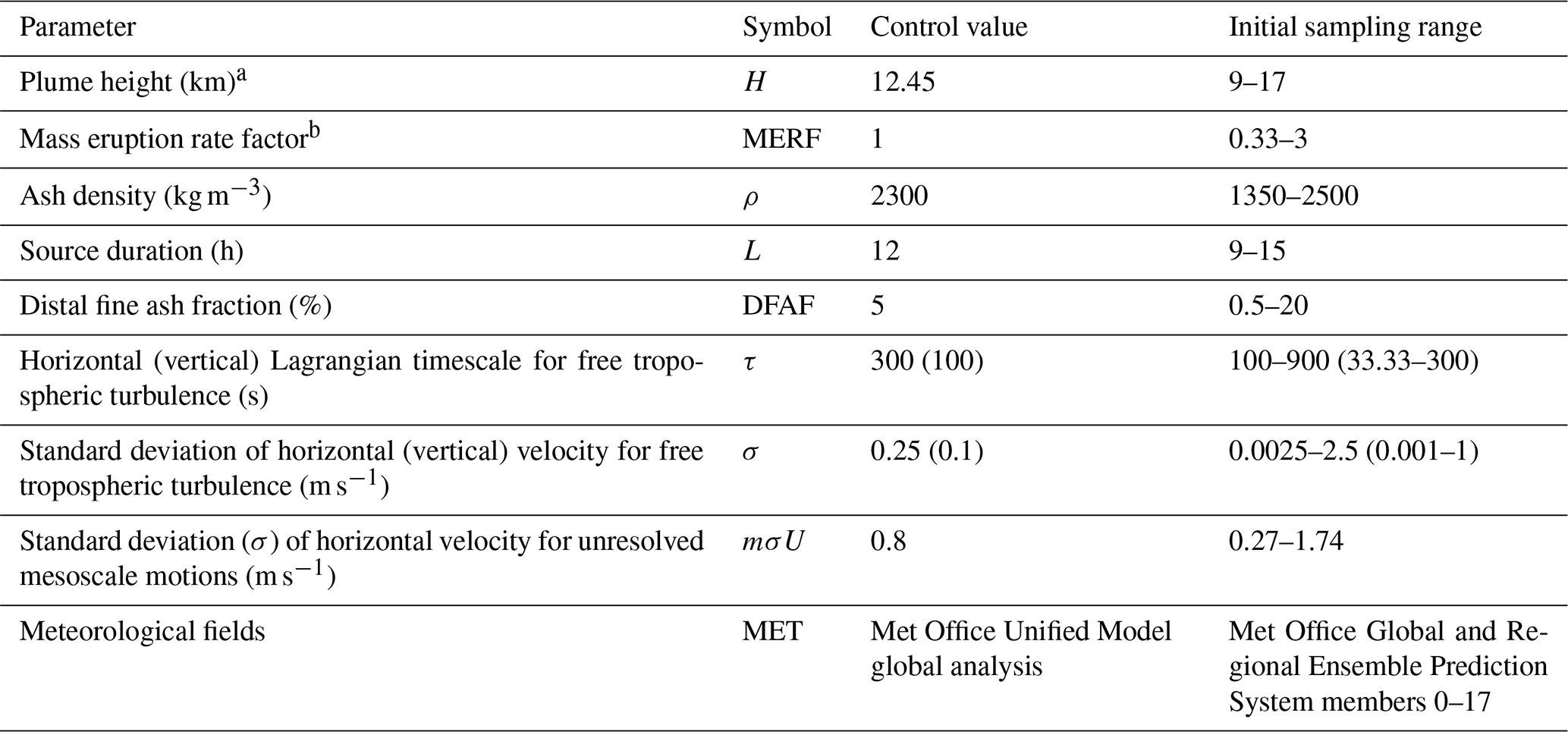
^a Plume rise height above the summit. ^b Scaling factor applied to the default mass eruption rate value calculated using the equation from Mastin et al. (2009); see Sect. 4.1.1 for details on how mass eruption rate is calculated.

3 Description of the 2019 Raikoke eruption

Raikoke is an uninhabited volcanic island near the centre of the Kuril Island chain in the Sea of Okhotsk in the northwest Pacific Ocean located at 48.2^∘ N, 153.3^∘ E. Its most recent explosive eruption, after 95 years of dormancy, started at approximately 18:00 UTC on 21 June 2019 and is estimated to have an initial eruptive plume height of 10–13 km above sea level (a.s.l.) (Global Volcanism Project, 2019). The eruption lasted approximately 12 h and ended at approximately 06:00 UTC on 22 June 2019. There is evidence from visible satellite imagery to suggest that there was an umbrella cloud that was quickly advected eastwards towards a large extratropical cyclone, which distorted the dispersed ash cloud (Fig. 1).

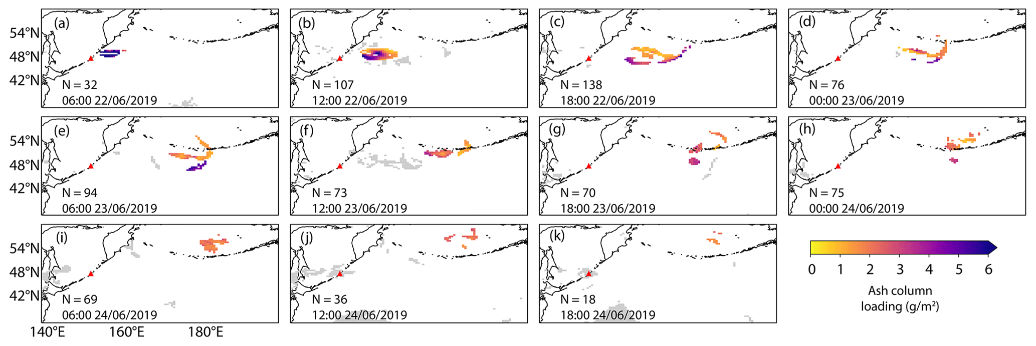
Figure 1 Hourly mean ash column loadings from the Himawari–8 satellite at (a) 06:00 UTC, (b) 12:00 UTC, (c) 18:00 UTC on 22 June 2019, (d) 00:00 UTC, (e) 06:00 UTC, (f) 12:00 UTC, (g) 18:00 UTC on 23 June 2019, (h) 00:00 UTC, (i) 06:00 UTC, (j) 12:00 UTC, (k) 18:00 UTC on 24 June 2019. Grey shading indicates grid boxes that are classified as clear sky. The red triangle indicates the location of Raikoke. N indicates the number of grid boxes classified as containing ash. The same colour bar applies to all maps.

The number of satellite grid boxes that are classified as containing ash at each time are the ones available to be used to refine the prior pdfs. The largest number of boxes are available at 18:00 UTC on 22 June. Before 06:00 UTC on 22 June, the number of grid boxes available is limited by the small time the ash has had to be transported. After 18:00 UTC on 24 June, the number of grid boxes is limited due to the presence of meteorological cloud associated with an extratropical cyclone situated to the east of Raikoke.

4 Particle filter construction

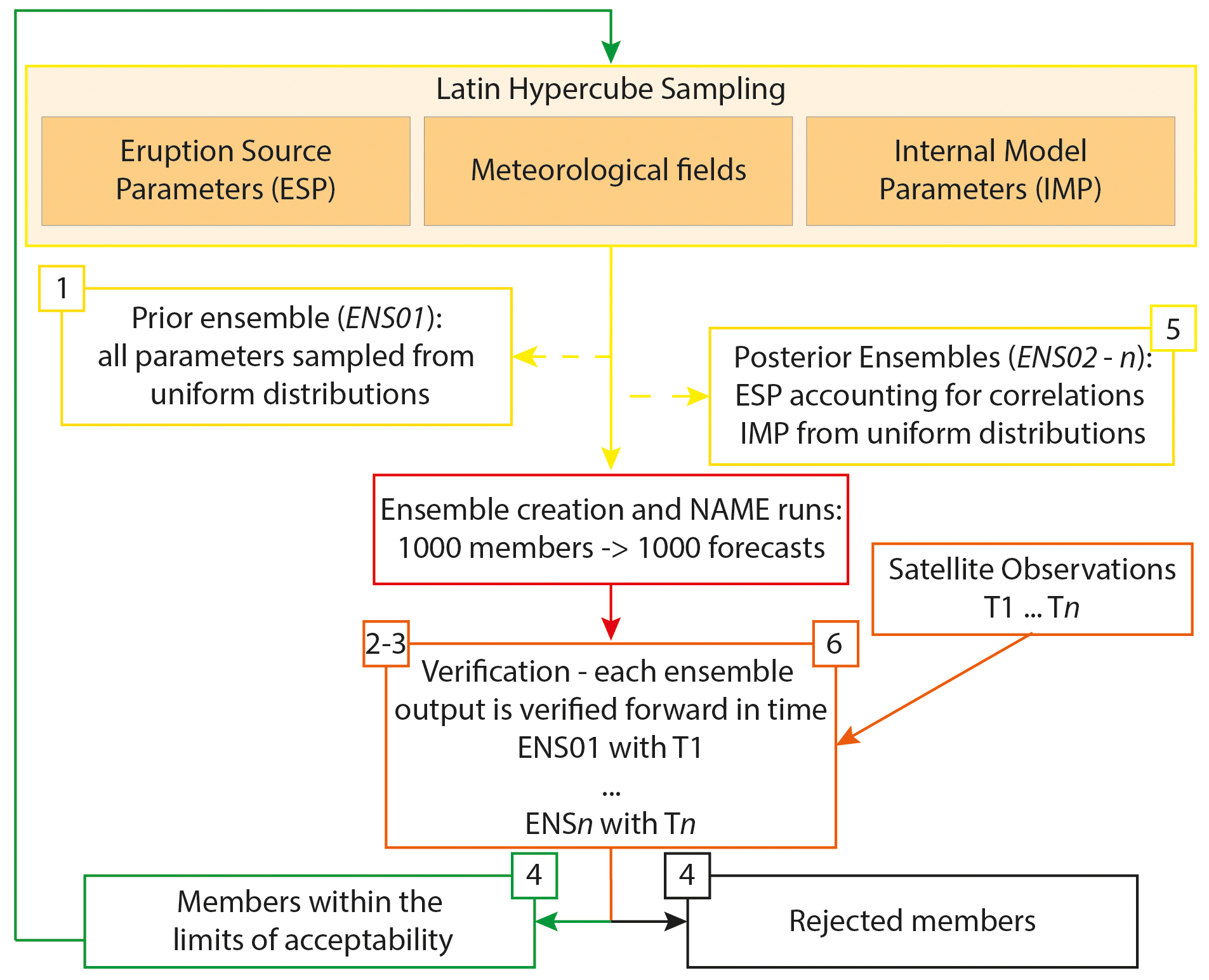
Drawing from the GLUE methodology described in Sect. 1, we developed a new particle filter for refining a series of ensembles moving forward in time based on their level of agreement with Himawari–8 satellite observations. All ensemble members are evaluated and filtered by comparing the NAME–simulated ash column loadings (g m⁻²) with the satellite–detected ash column loadings (g m⁻²) for a given analysis time. Column loading retrievals from Himawari–8 cover a time range from 18:00 UTC on 21 June 2019 to 00:00 UTC on 24 June 2019. However, due to the low number of grid boxes containing ash before 18:00 UTC on 22 June (Fig. 1), for the initial ensemble (ENS01) we chose as first verification time, T₁, the observations at 06:00 UTC on 22 June 2019. For this given time, 32 grid boxes containing ash are available (Fig. 1). Each satellite hourly average represents an average of data available at two times for each hour of the observation (e.g. for 06:00 UTC on 22 June 2019, the satellite observations are an average of data from 06:00 and 05:30 UTC). Comparing NAME-simulated ash column loadings with observations that had been time-averaged over 1, 3, or 6 h showed little change with averaging duration. However, averaging over longer periods led to a decrease of the number of grid boxes available for comparison for some of the observations. Therefore, we retained 1 h average observations for comparisons.

The particle filtering operation is designed such that, once all the members of an ensemble have been evaluated based on user defined rejection criteria, only those within the limits of acceptability are retained and used to produce posterior pdfs. A posterior ensemble is created by re-sampling the perturbed parameters from the posterior pdfs, which are then compared forward in time with a new set of observations, T_n. Therefore, each posterior ensemble represents a new possible state of our simulated ash cloud at a future time based on the evaluation performance of the prior ensemble at a previous time. The main steps involved in the methodology are summarised (Fig. 2):

1. Prior pdfs are created for the nine perturbed parameters, including eruption source parameters, driving meteorology, and NAME model internal parameters (Table 1; Fig. 2). We assign an initial range for each parameter that is then sampled independently from a uniform distribution to create an ensemble of 1000 members, ENS01. Perturbed parameters and their initial ranges are detailed in Sect. 4.1.

2. We define our rejection criteria, based on the threshold values for our verification metrics: Hit Rate (HR) and Mean Percentage Difference (MPD). Section 4.2 describes how we calculate HR and MPD and how we set the thresholds (Fig. 2).

3. Each model prediction from ENS01 is compared with the satellite observations at a given time, T₁. All posterior ensembles are verified at a future time using observations every 6 h (Fig. 2)

   $$\begin{array}{c}{\displaystyle }\mathrm{ENS}\mathrm{01}\to T_{\mathrm{1}}=\text{22 Jun 2019, 06:00\hspace{0.17em}UTC},\\ {\displaystyle }\mathrm{ENS}\mathrm{02}\to T_{\mathrm{2}}=\text{22 Jun 2019, 12:00\hspace{0.17em}UTC}\\ {\displaystyle }\mathrm{\dots }\\ {\displaystyle }\mathrm{ENS}n\to T_n=T_{n-\mathrm{1}}+\mathrm{6}\mathrm{h}.\end{array}$$

4. Simulations that, based on the rejection criteria, are not in agreement with the satellite observations are discarded. The retained simulations are used to form the posterior pdfs for each input and internal model parameter (Sect. 4.3; Fig. 2).

5. Posterior pdfs are generated from the parameter sets of the retained simulations, also considering possible interaction among them by including effects of covariation between eruption source parameters. Parameters are re-sampled from these posterior pdfs, creating a new 1000-member posterior ensemble (Fig. 2). The newly created posterior ensemble represents a possible state of our system at a future time (Sect. 4.3). Each member of the new ensemble produces a new 96 h forecast, from 18:00 UTC on 21 June 2019 to 12:00 UTC on 25 June 2019.

6. Each model prediction from the posterior ensemble is compared forward in time with a new set of satellite observations (Table 2; Fig. 2).

7. Steps 4–6 are repeated until all the available satellite observations are covered.

Figure 2 Overall workflow of the particle filtering methodology.

4.1 Ensemble creation

Each ensemble of NAME simulations is created by perturbing nine parameters, including eruption source parameters, driving meteorology, and internal NAME parameters. To generate the ensemble efficiently, we use Latin hypercube sampling (LHS), which covers our entire parametric space maintaining orthogonality among the different perturbed parameters (Prata et al., 2019). For ENS01, each parameter in the LHS is chosen from prior pdfs, which ranges are defined by a set of minima and maxima (Table 1) and sampled from a uniform distribution assuming that all values within these ranges are equally likely. For each posterior ensemble, the ESPs in the updated LHS designs are chosen from the posterior pdfs, while NAME internal parameters and members of the Met Office Global and Regional Ensemble Prediction System (MOGREPS-G) forecasts continue to be sampled from uniform distributions (Sect. 4.3).

4.1.1 Eruption source parameters (ESPs)

To represent an initial uncertainty associated with ESPs for ENS01, we define a minimum and a maximum possible value for each perturbed parameter. Then, a parameter value is sampled from a uniform distribution across this range.

We selected a total of five ESPs to perturb from those that have been shown to have most effect on the simulated ash cloud (e.g. Harvey et al., 2018; Prata et al., 2019): plume height (H), distal fine ash fraction (DFAF), mass eruption rate factor (MERF), ash density (ρ), and eruption duration (L). H is used to calculate the mass eruption rate (MER) for each member using the empirical relationship from Mastin et al. (2009). For each ensemble member, MER is scaled by the DFAF, representing the percentage of ash transported at long distances, and multiplied for the MERF, to account for uncertainties associated with the Mastin et al. (2009) relationship. Hence, MER is not perturbed explicitly.

Plume height

Plume height (H) constrains the lower and upper limits of the ash particles' release height and, therefore, significantly impacts both the vertical and horizontal structure of the simulated ash cloud. Although the Raikoke eruption was characterised by the formation of an umbrella cloud, in NAME, ash release is defined as a vertical line along which the ash is uniformly distributed, with the lower and upper bounds representing the volcano summit height (551 m a.s.l.) and the reported plume height, respectively. We based our initial H range on information available at that time. The Kamchatkan Volcanic Eruption Response Team (KVERT) and the Tokyo and Anchorage VAAC reported a large ash plume extending from 10 to 13 km (a.s.l.) within the first few hours of eruption (Global Volcanism Program, 2019), while data from CALIPSO satellite indicate that the plume may have reached altitudes up to 17 km (a.s.l.; Hedelt et al., 2019). For our initial ensemble, we selected H ranges between 9–17 km (a.s.l.) and for the control run, we set H = 13 km (a.s.l.; Table 1).

Mass eruption rate (MER)

The mass eruption rate, MER, is estimated from the plume height using the empirically derived relationship from Mastin et al. (2009)

$$\begin{array}{}\text{(1)}& \mathrm{MER}=\mathrm{50.7}\times {\mathrm{10}}^{\mathrm{7}}{H}^{\mathrm{2}/\mathrm{0.241}},\end{array}$$

where H represents the plume height in km. MER is expressed in g h⁻¹. By calculating the MER from H, any uncertainty associated with H propagates in the resulting MER calculation. Furthermore, there is also an uncertainty associated with the nature of the relationship, being an empirical one and based on a relatively small number of eruptions of variable magnitude (Mastin et al., 2009). In order to take this into consideration, for all the ensemble members, the MER is perturbed for a factor between 0.33 and 3, while we use 1 for the control run (Mass Eruption Rate Factor, MERF; Harvey et al., 2018; Prata et al., 2019; Table 1).

Distal Final Ash Fraction (DFAF)

The MER calculated with the Mastin et al. (2009) relationship (Eq. 1) estimates the total mass released during an eruption. However, the particle size distribution (PSD) of the erupted particles includes both larger particles (>1 mm) that are usually removed from the column in the first phases of an eruption and an additional finer fraction that may leave the column due to aggregation processes. Particles larger than 100 µm are removed rapidly, without travelling long distances, and as result, only a fraction of fine particles <100 µm is transported at long distances. Details of the true PSD are often unknown. Here, the default LVAAC PSD is used in each simulation (Table 1 in Witham et al., 2019), and aggregation processes are not modelled in the NAME simulations for this study. To account for this, the model assumes that most of the ash falls out close to the volcano, with only a small percentage of it reaching the distal plume. The NAME default value for this percentage (distal fine ash fraction, DFAF, Dacre et al., 2011), used here for the control run, is 5 %; however, the real value is uncertain and varies with each eruption (Witham et al., 2019). Consequently, the uncertainty associated with DFAF can be very high (Grant et al., 2012). Recent studies challenged the 5 % assumption by reaching contrasting conclusions: either 5 % is too high for most of the eruptions (Gouhier et al., 2019), or it is too low, severely underestimating mass loadings (Cashman and Rust, 2020). For our prior ensemble, the range used is 0.5 %–20 % (Table 1).

Ash density

The default LVAAC value for particle density is 2300 kg m⁻³ (Witham et al., 2019) and particle shape is assumed to be spherical in the NAME simulations. At the time of writing, no specific ash density or shape information is available for the 2019 Raikoke eruption. Density was selected as parameter to perturb as it may help in representing uncertainty attributed to ash aggregation and particle shape (e.g. Harvey et al., 2018). The range used is 1350–2500 kg m⁻³, while we use the default 2300 kg m⁻³ for the control run (Table 1).

Source duration

The overall duration of the intense phase of the Raikoke eruption is relatively well constrained, with KVERT reporting a strong explosive eruption beginning about 18:05 UTC on 21 June and a weaker explosive event reported at 05:40 UTC on 22 June. However, ash emission continued, possibly until around 08:00 UTC on 22 June, when KVERT reported a gas–steam plume with some ash content (Global Volcanism Program, 2019). As uncertainty in the duration of ash emission may lead to uncertainty in both the location and timing of the modelled ash cloud (e.g. Prata et al., 2019), we considered a duration range of 9–15 h for ENS01 and 12 h for the control run (Table 1). In the simulations, eruption source parameters are assumed constant throughout the release duration, although this is unlikely to be true for the Raikoke eruption.

4.1.2 Driving meteorology

In this study, NAME was driven by the operational forecasts from MOGREPS-G. The global forecasts have 17 ensemble members plus a control member. The horizontal resolution is approximately 20 km in the mid-latitudes, and there are 70 vertical levels with the lid at approximately 80 km. Each forecast is run out for 7 d, and they are initialised four times per day at 00:00, 06:00, 12:00 and 18:00 UTC (Bowler et al., 2008). At the time of the Raikoke eruption, MOGREPS–G used an on-line inflation factor calculation to calibrate the spread of the ensemble in space and time and a stochastic physics scheme to account for model uncertainty (Flowerdew and Bowler, 2011, 2013). The MOGREPS–G forecasts used in this study were initialised at 12:00 UTC 21 June 2019.

4.1.3 NAME internal model parameters

Previous studies have demonstrated how the NAME internal model parameters used for representing the free tropospheric turbulence can significantly impact the model output as they affect the vertical thickness of the simulated cloud and the overall motion of particles (Dacre et al., 2015; Harvey et al., 2018; Prata et al., 2019). To represent uncertainty in free tropospheric turbulence, we perturb the standard deviation (σ) and Lagrangian timescales (τ) of the horizontal and vertical velocity components in NAME, by sampling them from a uniform distribution using the same ranges specified in Harvey et al. (2018) and Prata et al. (2019), with the horizontal component of σ sampled on a logarithmic scale. The horizonal and vertical components of these parameters are varied in proportion to each other. Similarly, σ of the horizontal velocity for unresolved mesoscale motions is also varied using the same range as in Harvey et al. (2018) and Prata et al. (2019) and sampled from a uniform distribution. For the control run, we use the default NAME values (Table 1). For both the control run and the ensembles, these values are fixed in time.

4.2 Particle filter verification metrics

Each simulation is either discarded or retained based on its level of agreement with the satellite retrievals. We restrict the comparison only to the area covered by both NAME simulated ash cloud and by detectable ash in the satellite observations. The comparison is performed based on two verification metrics: hit rate (HR) and mean percentage difference (MPD).

4.2.1 Step 1: Identifying matching pixels

Most satellite retrievals are unable to detect column loadings less than 0.2 g m⁻² (Prata and Prata, 2012). Consequently, before comparing the Himawari–8 data and NAME output (Fig. 3a and b), we apply a minimum threshold of 0.2 g m⁻² to the NAME-simulated ash column loading to align with the minimum detection limit of the satellite observations. The Himawari-8 observations and their error are both re-gridded over the NAME horizontal grid, to facilitate inter comparisons. The re-gridding process is performed using IRIS (Met Office, 2021). There was no noticeable difference between re-gridding either each ensemble member based on the satellite grid, or each observation and its error based on the NAME grid, using the different re-gridding schemes available. However, re-gridding each ensemble requires long computational times. Therefore, we decided to re-grid the observation and its error based on NAME as target grid, using an area-weighted re-gridding scheme (Met Office, 2021). Finally, we identify the grid boxes in which both the NAME output and the satellite retrievals detect ash as “matching pixels” (Fig. 3c). For each ensemble member, we then calculate the hit rate and mean percentage difference based on all matching pixels.

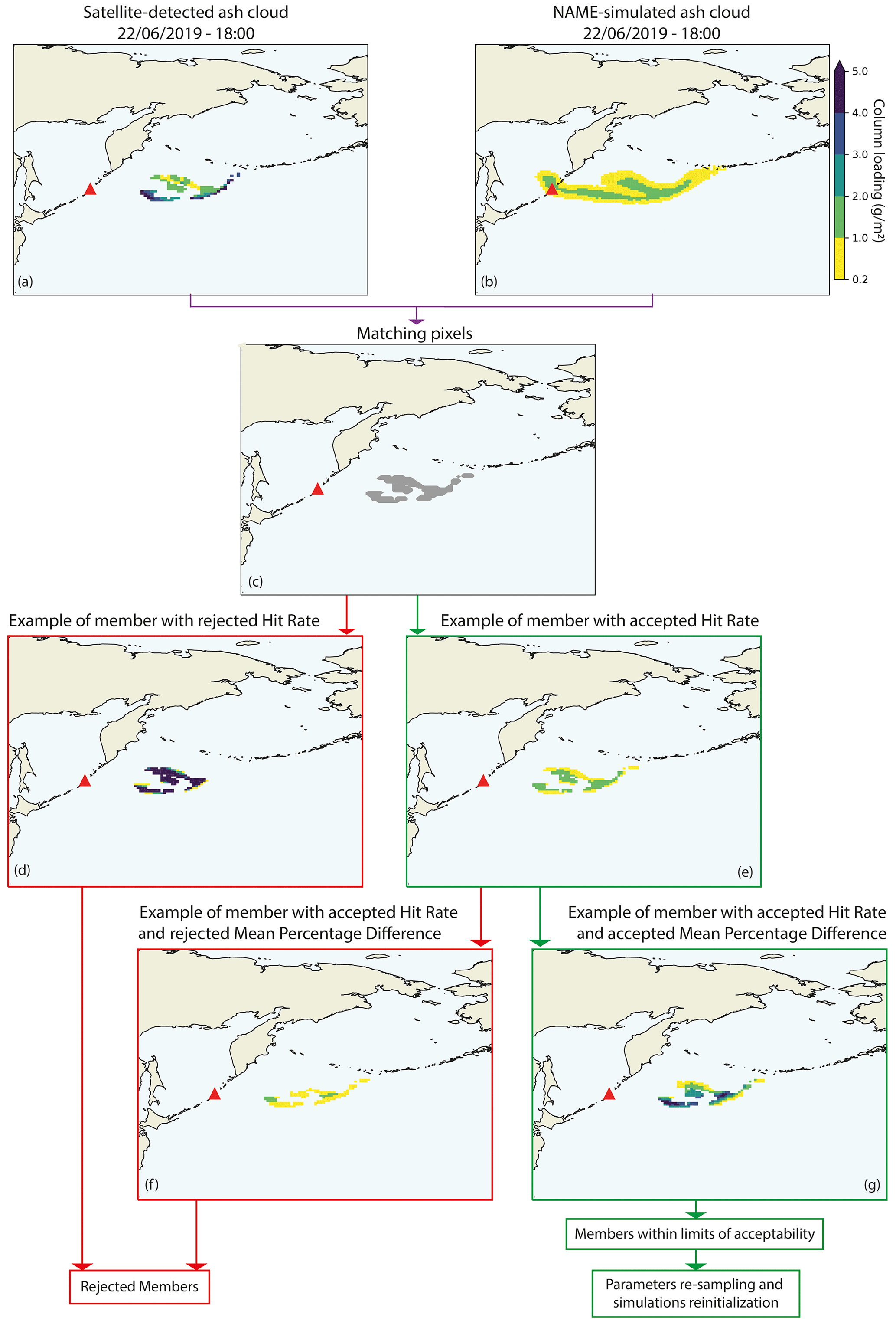
Figure 3 Ash column loading at 18:00 UTC on 22 June 2019, (a) as detected by the satellite, (b) NAME simulation of one ensemble member in NAME, and (c) after pixel-matching (grey pixels represent a match between satellite and simulation). Examples of ensemble members rejected depending on values of hit rate and mean percentage difference (red boxes) are shown in (d) and (f). Examples of accepted ensemble members depending on values of hit rate and mean percentage difference (green boxes) are shown in (e) and (g). All panels except (c) use the colour scale shown in (b). The red triangle in each panel shows the location of Raikoke.

4.2.2 Step 2: Calculating the hit rate

The hit rate, HR, is a widely used categorical metric applied to many meteorological phenomena for forecast verification, representing the proportion of observed events that are successfully forecast by a simulation. HR can be used to discriminate “yes events” and “no events”, often by specifying a threshold to separate “yes” and “no” (Joliffe and Stephenson, 2012). Similarly, HR has also been used to provide information on how ash forecast model outputs compare to observations in terms of binary ash yes/ash no events (e.g. Stefanescu et al., 2014; Marti and Folch, 2018). In such cases, a grid box would represent a hit if both simulation and observation detected ash above a threshold of >0.2 g m⁻².

Here, we calculate the hit rate as the percentage of matching pixels for which the simulated value lies within one standard deviation of the corresponding mean satellite-detected ash column loading. The standard deviation is provided by the retrieval algorithm as a measurement of the error for the retrieved ash values in each grid box (Sect. 2.1). Hence, we both directly compare the ash column loadings between simulation and observations for each individual matching pixel, and we complement this by considering the error associated with the satellite observations.

Once we have identified the total number of hits in each member, HR can be calculated

$$\begin{array}{}\text{(2)}& \mathrm{HR}={\displaystyle \frac{\mathrm{HITS}}{\mathrm{Matching}\mathrm{Pixels}}}\times \mathrm{100}.\end{array}$$

At this point, members that have an HR below a specific threshold are discarded (Sect. 4.2.4; Fig. 3d) and the remaining members (Fig. 3e) are then verified further by testing against the observations using mean percentage difference.

4.2.3 Step 3: Calculating the mean percentage difference

The final step in the evaluation process determines, for the members retained following the HR verification, how much the NAME–simulated ash column loading values differ from the satellite–detected ones on a grid box basis. The percentage difference magnitude (PD) for each matching pixel is the absolute value of the difference between the simulated and observed column loadings, divided by the mean of the two values and expressed in terms of percentage.

Then, the mean of the PDs over all grid boxes (MPD) for each ensemble member is calculated. Ensemble members with MPD below a threshold (Sect. 4.2.4; Fig. 3g) are retained and used to form our posterior. Those above the threshold are rejected (Fig. 3f).

4.2.4 HR and MPD thresholds

Both HR and MPD are sensitive to the total number of satellite grid boxes containing detectable ash. Therefore, when there are only a few satellite grid boxes available, fixed HR and MPD thresholds may retain too few ensemble members to form posterior pdfs. As our verification method is based on limits of acceptability, to avoid a situation where either all simulations are rejected or too few members are retained for re-sampling, we implemented dynamic thresholding for both HR and MPD. The acceptability thresholds for HR and MPD are adjusted dynamically during the verification to ensure that a minimum of 50 ensemble members is retained (i.e., 5 % of total number of ensemble members). This dynamic adjustment is carried out by initially setting the HR threshold to 95 % and the MPD threshold to the minimum MPD value. Ensemble members are evaluated against these thresholds, and the thresholds adjusted (by increasing the MDP value up to the median value, and by decreasing the HR value, in 5 % increments) until at least 50 members lie within the limits of acceptability.

This dynamic thresholding method, therefore, guarantees that the members within limits of acceptability are always retained using the “best” threshold available for both HR and MPD, for a given time (Table 2). Only for T₁, when 32 grid boxes containing detectable ash are available, were both thresholds varied substantially, and fewer than 50 members were retained. Thereafter, a HR of 95 % was maintained at each verification cycle. MPD values had to be varied more to retain at least 50 members but were always within the range 20 %–50 % of the minimum MPD.

Table 2 Number of members within limits of acceptability (WLoA), and HR and MPD thresholds for each ensemble at each verification time.

^a Total number of retained ensemble members for a given time. Parameters for Ensemble 01 (prior ensemble) were sampled from uniform distributions. Parameters for each subsequent ensemble (posterior ensemble) were sampled from posterior pdfs obtained from the retained members of the previous ensemble, verified at the previous verification time. Threshold values for HR (higher is better) and MPD (lower is better) used at each verification time are shown in the last two columns. ^b Total number of ensemble members that would be retained from the prior ensemble, ENS01 if the verification was run at each verification time, using the same HR and MPD thresholds for which each posterior ensemble has been evaluated.

4.3 Posterior re-sampling

The comparison of the prior and posterior pdfs for each parameter allows us to identify the range of parameters that represent a good approximation of those generating the observed volcanic ash cloud at the verification time. Figure 4 shows this comparison for ENS01, ENS02, ENS03, and ENS04; each ensemble was verified using observations at T₁, T₂, T₃, and T₄, respectively (Table 2). For ENS01 (Fig. 4a), most of the ESP pdfs from the retained simulations are highly skewed. In particular, this can be seen for H, DFAF, and MERF. H is used to calculate the mass eruption rate (shown in Fig. 4 but not explicitly perturbed), which is then perturbed further by DFAF and MERF. Therefore, these ESPs significantly influence both the vertical and horizontal structure of the modelled ash cloud and ash concentrations. However, ENS02 (Fig. 4b), ENS03 (Fig. 4c), and ENS04 (Fig. 4d), which use the particle filter described above, show how as more ensembles are run and evaluated forward in time with new observations, the parameter ranges of each posterior ensemble gradually reduce. Additionally, the differences between posterior pdfs and the prior pdfs decrease, and the ESPs become increasingly constrained.

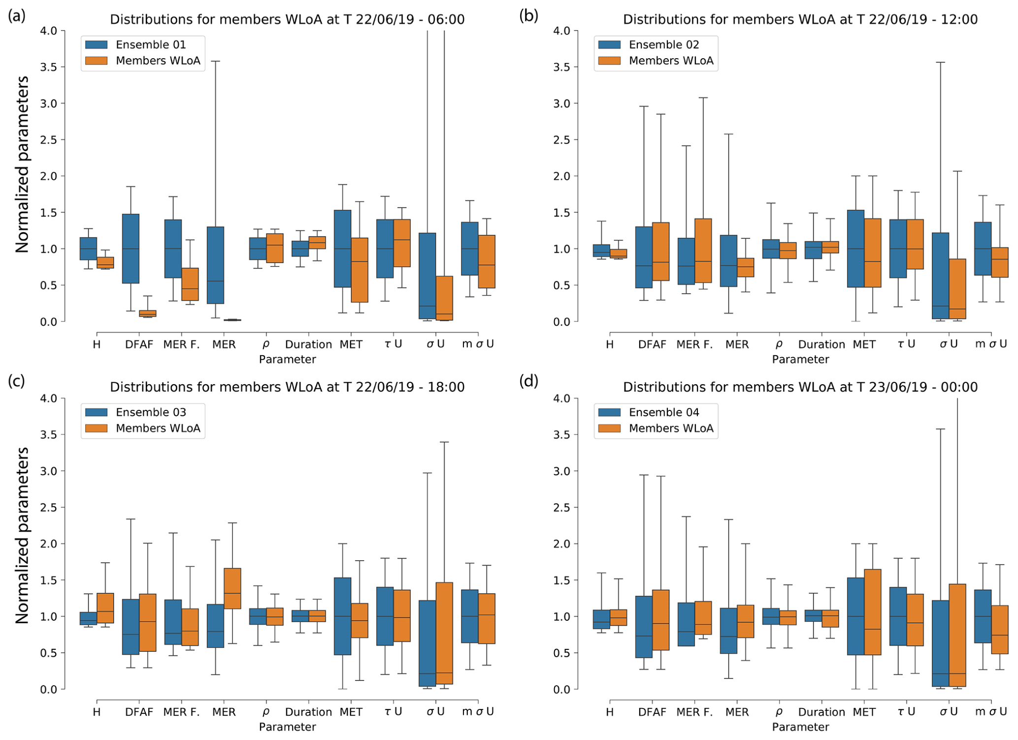
Figure 4 Evolution of parameter distributions for members within limits of acceptability (WLoA) for (a) Ensemble 01, (b) Ensemble 02, (c) Ensemble 03, and (d) Ensemble 04. ρ, τU, σU, and mσU represent density, horizontal Lagrangian timescale for free tropospheric turbulence, standard deviation of horizontal velocity for free tropospheric turbulence, and standard deviation (σ) of horizontal velocity for unresolved mesoscale motions. In (a), (b), (c), and (d), the mass eruption rate (MER) is plotted to show its variation, although it is not explicitly perturbed in any of the ensembles. Each parameter in the box plots is normalised by dividing each individual value from the ensemble members by the mean of that entire parameter range from the selected ensemble. The evolution of parameters distributions for ENS05–ENS11 are shown in Appendix A (Fig. A1).

Although this evolution is evident for many of the ESPs, the input model parameters (τU, σU, and mσU) do not show a similar behaviour among the different ensembles. This seems to hold for all the 11 ensembles (Figs. 4 and A1 in Appendix A), suggesting that the Raikoke simulations are not sensitive to these internal parameters.

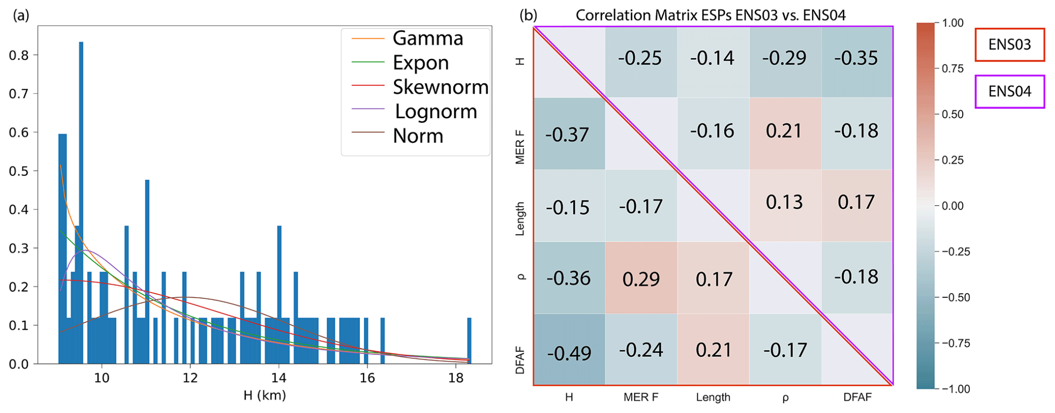
Figure 5 (a) Example of distribution identification for fitting plume height (H) from members WLoA of ENS03 and (b) comparison of correlation matrices between ENS03 ESPs in the members WLoA (lower matrix, red triangle) and ESPs posterior pdfs for ENS04 (upper matrix, purple triangle).

This constraining behaviour is the result of the refinement of each posterior ensemble, achieved by repeatedly refitting the parameters sets of the retained simulations at each verification time, and re-sampling posterior ensemble parameters from the newly fitted posterior pdfs. For the prior ensemble, the LHS is performed independently for each parameter. However, eruption source parameters are likely to be correlated, especially the plume height, distal fine ash fraction, and mass eruption rate factor, which are used to estimate and perturb the mass eruption rate. Thus, we want to maintain dependency among the ESPs during the re-sampling process. The main steps of this process are the following:

1. The input parameter ranges from the retained members are fitted with a gamma distribution (which represented the overall best-suited distribution, Fig. 5a) and used to generate a correlation matrix for the ESPs (Fig. 5b).

2. A new LH design is created (1000 samples for 5 parameters), and each sample is mapped to values applying inverse cumulative distribution function (CDF) of a normal variable N(0,1). The generated values are independent and follow a normal distribution.

3. Using a Cholesky decomposition of the correlation matrix, a correlation structure is enforced to the new LHS design, adding dependency to the normal values of our parameters.

4. Finally, by applying a normal CDF to the normal variables, we transform them into uniform random variables, and then map the uniform distribution to the specified distribution function (gamma), applying the inversion CDF of our gamma distributions.

Each ESP is sampled from the newly generated posterior pdfs in the updated LHS design, therefore maintaining the dependency among the parameters (Fig. 5b). In contrast, as we did not observe the same constraining behaviour for the model input parameters and driving meteorology (Figs. 4 and A1), those parameters are treated independently, and their posterior pdfs are sampled again from uniform pdfs, using the same ranges as for the prior ensemble (Table 1).

For the majority of the ESPs in ENS02, this re-sampling strategy modifies the ESP distributions away from the initial uniform distribution of the prior ensemble to a distribution that is highly skewed towards the lower end of the initial range (Fig. 6). Then, as the posterior pdfs are refined by moving forward in time with new observations, the pdfs for some of the ESPs, such as particle density and duration, seem to approximate normal distributions (Fig. 6).

Figure 6 Evolution of ESPs distributions for ENS01 (purple shading), ENS02 (blue shading), ENS03 (orange shading), ENS04 (green shading), ENS05 (red shading), and ENS06 (dark purple shading). Each panel shows (a) plume height (H), (b) distal fine ash fraction (DFAF), (c) mass eruption rate factor (MERF), (d) mass eruption rate (MER), (e) ash density (ρ), and (f) eruption duration. For ENS01, each parameter is sampled from a uniform distribution. For ENS02–06, each parameter is sampled from posterior pdfs following a fit of the members WLoA and considering the interaction among the parameters. MER is plotted to show its evolution, although it is not explicitly perturbed in any of the ensembles. Dashed black lines in each plot represent the parameter value used for the control run. The evolution of ESPs distributions for ENS07–ENS11 are shown in Appendix B (Fig. B1).

5 Discussion

The particle filtering data assimilation technique described in Sect. 4 demonstrates how a series of ensembles of volcanic ash simulations can be successfully constrained based on the level of agreement between the simulation output and satellite retrievals. Each ensemble is verified forward in time with new retrievals. Compared to the parameter ranges used for the prior ensemble (Table 1), the range of eruption source parameters used to produce simulated ash clouds that represent a good approximation to the observed volcanic ash cloud reduces as the posterior ensembles become more constrained by the satellite retrievals.

The effects of the refinement on the posterior ensemble can be observed in probability of exceedance maps, given here for three different thresholds of ash column loadings, 0.2 g m⁻² (Fig. 7b), 2 g m⁻² (Fig. 7c), and 4 g m⁻² (Fig. 7d). The satellite retrieval at 18:00 UTC 22 June 2019 detects two distinct regions where ash loadings exceed 0.2 and 2 g m⁻² (Fig. 7a). The posterior ensemble (ENS03 – brown contour) agrees with the control run (black contour) and the prior ensemble (purple contour) on regions where loadings >0.2 g m⁻² are likely (30 %–60 %) and very likely (60 %–100 %; not plotted in Fig. 7). The simulated ash cloud regions are more extensive than the area of satellite-detected ash. However, this overestimation is greater for both the prior ensemble (ENS01 – purple contour) and the control run (black contour) than for the posterior ensemble (ENS03 – brown contour) and is largest for column loadings >2 g m⁻² (Fig. 7c) and 4 g m⁻² (Fig. 7d). The refined ensemble shows a much-reduced region with a 30 %–100 % probability of exceeding these loadings, showing better agreement with the observations especially when considering loadings > 2 g m⁻² detected by the satellite (Fig. 7a). Thus, by accounting for uncertainties, a wider region where those loadings are less likely has been shown instead, for all the considered thresholds (up to 30 %, dashed blue contour, not plotted in Fig. 7 but in Appendix C, Fig. C1).

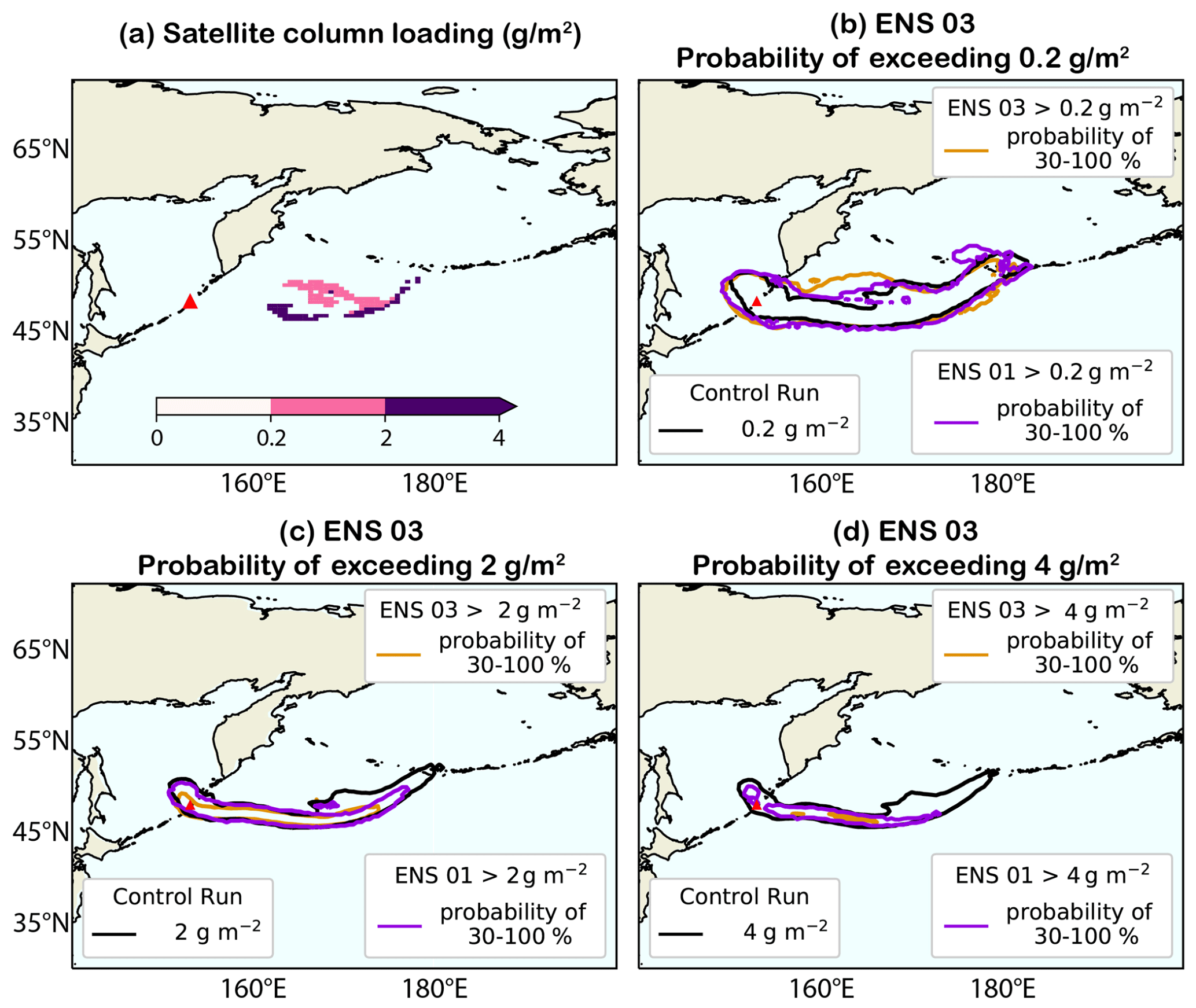
Figure 7 (a) Satellite-detected column loading at T₃ (22 June 2019 18:00 UTC) shown in filled contours. Probability of exceedance maps for ENS03 at T₃ for column loading thresholds of (b) 0.2 g m⁻², (c) 2 g m⁻², (d) 4 g m⁻² shown with dashed brown contour (30 % probability region – the region within the brown line goes from 30 % up to 100 %). The black contour in (b), (c), and (d) shows the relevant column loading threshold for the control run. The purple contours show the 30 % probability region for ENS01 of exceeding the relevant column loading threshold (the region within the purple line goes from 30 % up to 100 %). For generating the purple contours, members from the prior ensemble were retained by verifying ENS01 with observations at T₃ (a) and using the same HR and MPD thresholds for which ENS03 has been evaluated (Table 2) to ensure a fair comparison between the prior and posterior ensembles. See Fig. C1 in Appendix C for the same probability maps including the 0 %–30 % probability regions for ENS03.

By considering mean ash concentrations (mg m⁻³) at T₈ for ENS08, thus at 00:00 UTC on 24 June 2019, for the three “thick” flight layers, FL000–200 (Fig. 8a), FL200–350 (Fig. 8b), and FL350–550 (Fig. 8c), the control run seems to underestimate the areas with concentrations exceeding 0.2 mg m⁻³ compared to the subset of retained members of both ENS01 and ENS08. Contrariwise, ENS01 forecasts concentrations exceeding 0.2 mg m⁻³ over larger regions compared to the posterior ensemble. The overestimation increases considerably for FL200–350 but also for FL350–550, even with the posterior ensemble forecasting an additional plume tail extending to the east of Raikoke (Fig. 8c). Indeed, the areas forecasted by ENS08 with concentrations >0.2 mg m⁻³ for both FL200–350 (Fig. 8b) and FL350–550 (Fig. 8c) are, respectively, around 60 % and 30 % less extended than the ones forecasted by ENS01. In general, for all three flight levels, the area that a posterior ensemble would forecast with high ash concentrations is drastically reduced compared to the prior ensemble.

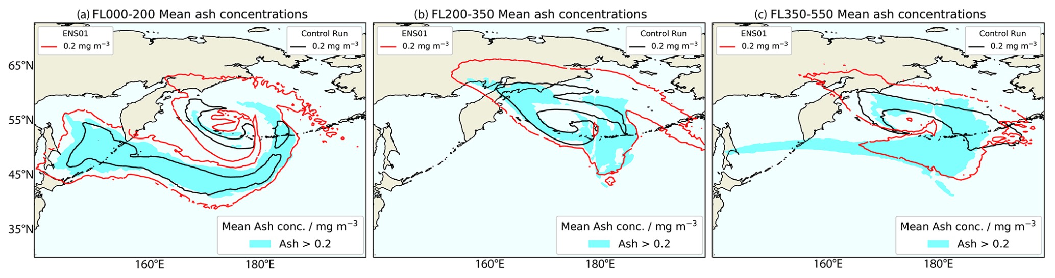
Figure 8 Mean ash concentration values >0.2 mg m⁻³ for ENS08 members (cyan region) for (a) FL000–200, (b) FL200–350, and (c) FL350–550 at 00:00 UTC 24 June 2019. Each panel shows also the associated 0.2 mg m⁻³ ash concentration contour for both the control run (black contour) and ENS01 (red contour).

5.1 Application to aviation operations

The use of probability of either exceedance maps (Fig. 7) or concentration maps (Fig. 8) condense the information given by the ensemble of VATDM simulations. However, multiple charts are still needed to cover all the relevant information, such as different flight levels, times, and ash concentration thresholds. To reduce information overload from these numerous charts, which could impede fast decision–making during emergency response, they can be condensed further into a single chart using a risk matrix (Prata et al., 2019). Here, we apply this risk-based approach to international flight routes in the vicinity of Raikoke using both the prior and posterior ensembles outlined in Sect. 4.

5.1.1 Flight routes and dosage risk

To simulate potential aircraft encounters with volcanic ash, flight routes with minimised travel time were generated by solving a time-optimal control problem as described in Wells et al. (2021). Trans-Pacific flights were generated assuming a constant true airspeed of 240 m s⁻¹ (∼ 864 km h⁻¹) at a cruise altitude of FL380 (or 200 hPa) and using horizontal wind speeds extracted from the National Center for Atmospheric Research re-analysis data (Kalnay et al., 1996). Eastbound and westbound time-optimal routes from Sapporo (CTS) to Honolulu (HNL), Los Angeles (LAX) to Seoul (ICN), and San Francisco (SFO) to Shanghai (PVG) international airports were calculated for each day of the dispersion model output (i.e., at 24 h intervals).

As in Prata et al. (2019), the along-flight ash dose, D, was defined as the ash concentration multiplied by the duration in that concentration (duration of exposure), integrated along an aircraft's flight path at cruise altitude (assumed to be FL350–550). This definition means that dose always increases monotonically along the route. All dose calculations assume that the modelled ash concentration fields at a given time step are fixed (i.e., do not change with time) as the aircraft flies from the origin to destination at its true airspeed (Prata et al., 2019).

5.1.2 Risk-based approach

The first step in determining the risk is to calculate the fraction of ensemble members that have concentrations above specified impact thresholds for each of the three flight levels. In line with the current International Civil Aviation Organisation (ICAO) guidance, the impact concentration thresholds used are 0.2–2, 2–4 mg m⁻³ and greater than 4 mg m⁻³, for low, medium, and high impact, respectively. The risk of encountering ash is then determined by combining the likelihood ranges (less likely, 0 %–10 %; likely, 10 %–90 %; very likely, 90 %–100 %) and the impact. The risk of flying in a specific location and at a flight level is then assigned to be low, medium, or high. The overall risk presented is the maximum risk over the three flight levels. In Prata et al. (2019), each risk level has a set of actions that may be implemented by the decision-maker. These range from checking updated ash forecasts to considering alternative routes and scheduling extra maintenance.

The risk can be visualised as a 2D map or projected on to flight tracks of interest (Fig. 9). Considering risk based on ash concentrations at 00:00 UTC on 24 June 2019, there are large portions of the flight tracks that encounter low and mid-level risk, with a small region of high risk to the east of Raikoke when using the prior ensemble (Fig. 9a). Thus, based on the prior ensemble output, flight operations could be expected to be severely disrupted at this time. However, determining risk from the posterior ensemble (ENS08) removes the region of highest risk and, overall, the amount of flight track potentially impacted and therefore requiring action from the flight operator is greatly reduced (Fig. 9b).

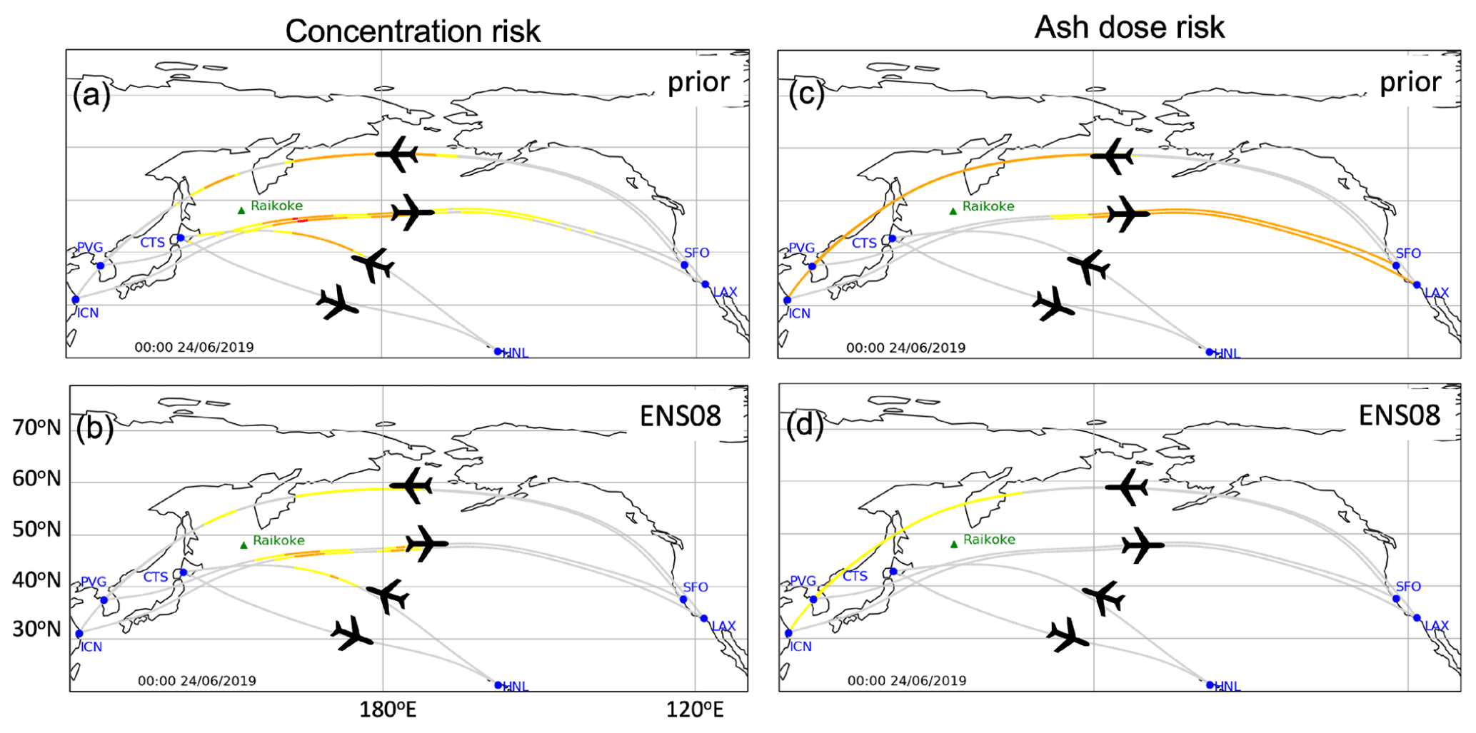
Figure 9 Concentration risk along time optimal flight routes at 00:00 UTC on 24 June 2019 for (a) prior ensemble (b) ENS08. Ash dose risk along the same time optimal flight routes at 00:00 UTC on 24 June 2019 for (c) prior ensemble (d) ENS08. Yellow shading indicates the lowest level of risk, orange shading indicates mid-level risk, and red indicates the highest level of risk. Note that dose risk only considers risk at FL350–550, whereas concentration risk considers at all levels.

To account for the overall exposure of the aircraft to ash, the risk approach can also be applied to dose along a flight track (Fig. 9). To do this the ash dose impact thresholds used are 4.4–14.4, 14.4–28.8 and greater than 28.8 g s m⁻³ (Clarkson and Simpson, 2017; Prata et al., 2019). The likelihood ranges used are the same as those used for the concentration approach. In this scenario, the risk is only determined at cruising altitude, which is assumed to be at FL350–550 (not the maximum over all flight levels). For the prior ensemble, the flight tracks to and from the West Coast of North America encounter mid-level risk and could potentially require specific actions by the airlines (e.g. more fuel and engine checks). Using this metric, flights between Honolulu and Sapporo do not reach doses that reach the lowest level of risk (Fig. 9c). For the posterior ensemble (ENS08), only the route from SFO to PVG and ICN reach sufficiently high doses to be highlighted by the risk approach. The other routes have very few ensemble members where doses are above 4.4 g s m⁻³ and therefore are not highlighted by the risk approach (Fig. 9d). This could greatly reduce the need for an operator to implement any mitigation strategies.

6 Conclusions

This study presents a new particle filtering data assimilation system that combines VATDM simulations with satellite retrievals including their uncertainty estimates, to improve forecasts of volcanic ash cloud location and concentration. A prior ensemble is created by simultaneously varying nine parameters representing the meteorology, eruption source, and internal parameters. Members from the prior ensemble are retained or discarded based on their level of agreement with the satellite retrievals. The retained simulations are then used to create a posterior ensemble. Each posterior ensemble is verified and filtered using satellite data at subsequent verification times.

The ESPs ranges in the constrained posterior ensembles are both smaller and skewed towards lower values than those used in the control run and prior ensemble, with the exception of ash density and eruption duration. Therefore, a single ensemble designed with unconstrained parameters ranges (i.e., the prior ensemble) seems insufficient for estimating ESPs ranges that may approximate more accurately the observed volcanic ash cloud. This is not the case for internal model parameters, which remain unconstrained by the data assimilation.

Communicating the risk of volcanic ash to aviation using risk maps and risk trajectories shows that the prior ensemble forecasts mid-level and highest risk for both ash concentration and dose thresholds for much of a set of representative flight tracks. Based on this information flight operations could be severely disrupted by the eruption. However, using the constrained posterior ensemble, the region of highest risk is removed, and the mid-level risk is reduced. Thus, using the refined posterior ensembles potentially reduces the need for the operator to implement any mitigation strategies and hence reduces disruption to airline operations.

This methodology is easily generalisable to other VATDMs and could be used to run a comparison with other models. Different remote sensing datasets could be used to assess its sensitivity to the observations used. Running multiple 1000-member ensembles requires either a high computational power or can be subject to variable queuing times on computer clusters such as JASMIN. Future work could include code optimisation to make runtime and ensemble size more efficient, potentially allowing an operational application. With a more manageable ensemble size, it could also be possible to introduce temporal variation of perturbed parameters, such as plume height, within each simulation. Furthermore, the evaluation method is based on limits of acceptability; a future improvement would be to define the posterior by weighting each simulation output according to some measure of its fit to the observations, in a way that takes proper account of the epistemic uncertainties in the satellite retrievals or any other available information.

Appendix A

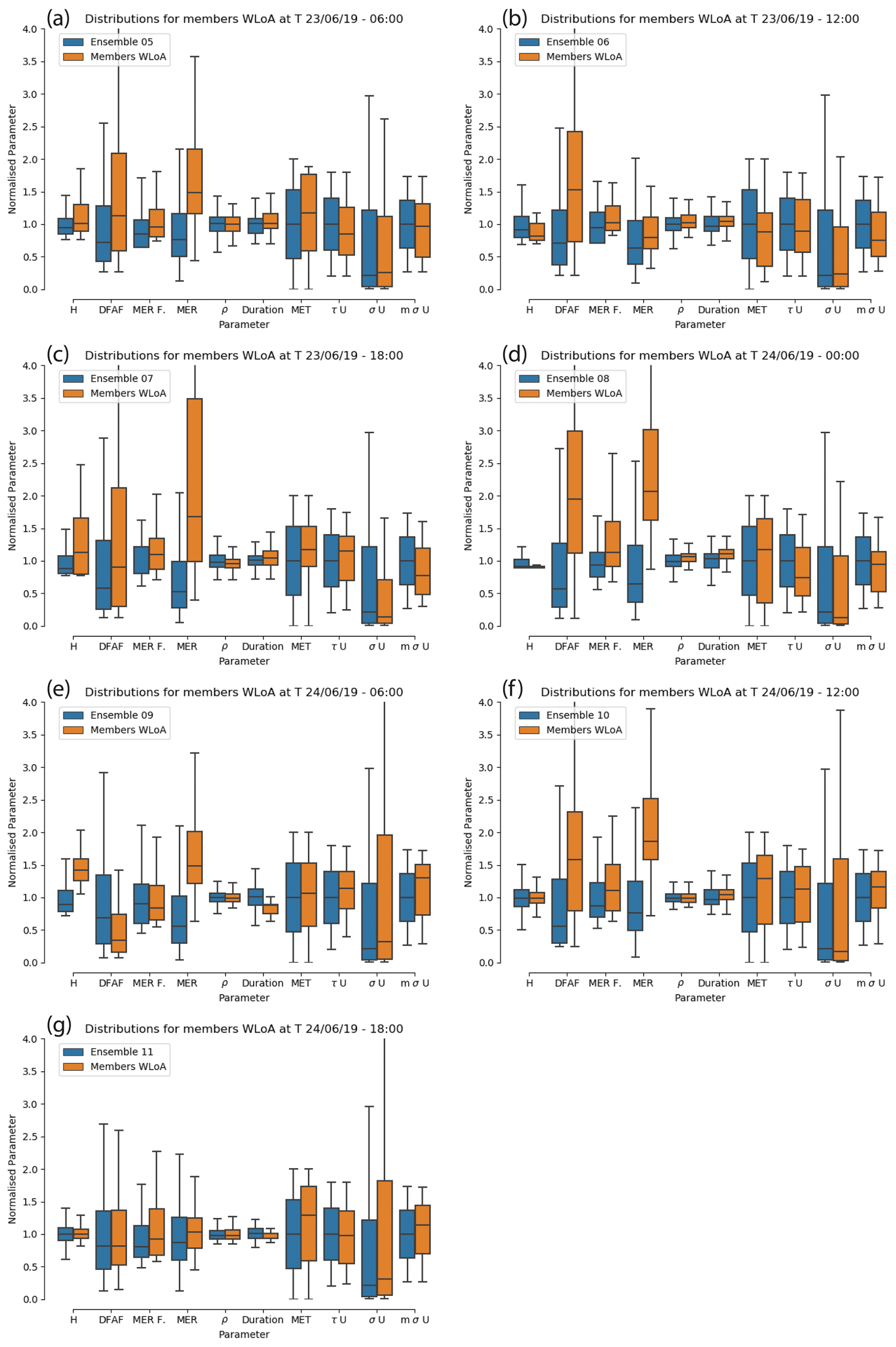
Figure A1 Evolution of parameters distributions for members within limits of acceptability (WLoA) for (a) Ensemble 05, (b) Ensemble 06, (c) Ensemble 07, (d) Ensemble 08, (e) Ensemble 09, (f) Ensemble 10, and (g) Ensemble 11. ρ, τU, σU, and mσU represent density, horizontal Lagrangian timescale for free tropospheric turbulence, standard deviation of horizontal velocity for free tropospheric turbulence, and standard deviation (σ) of horizontal velocity for unresolved mesoscale motions. In all panels, the mass eruption rate (MER) is plotted to show its variation, although it is not explicitly perturbed in any of the ensembles. Each parameter in the box plots is normalised by dividing each individual value from the ensemble members by the mean of that entire parameter range from the selected ensemble.

Appendix B

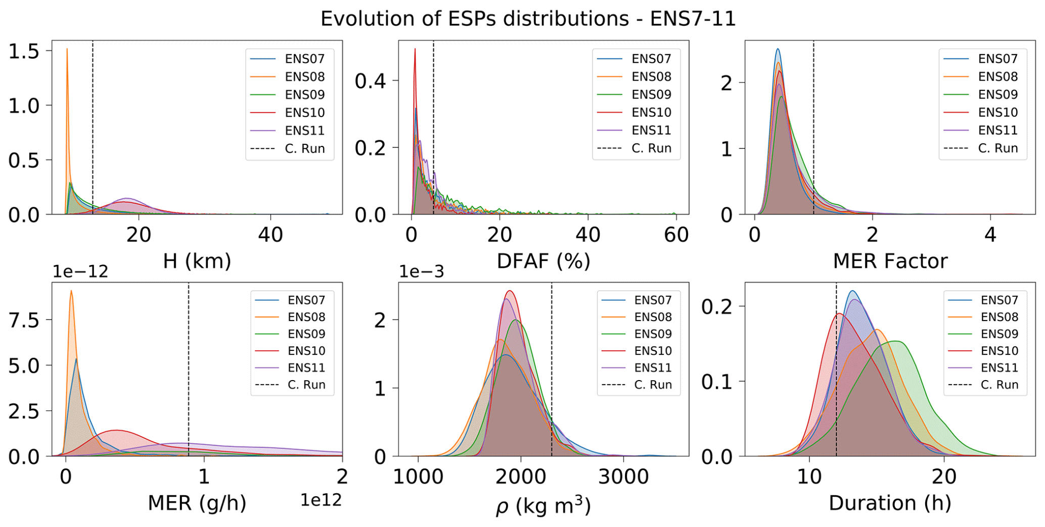
Figure B1 Evolution of ESPs distributions for ENS07 (blue shading), ENS08 (orange shading), ENS09 (green shading), ENS10 (red shading), and ENS11 (purple shading). Each panel shows (a) plume height (H), (b) distal fine ash fraction (DFAF), (c) mass eruption rate factor (MERF), (d) mass eruption rate (MER), (e) ash density (ρ), and (f) eruption duration. For ENS07–11, each parameter is sampled from posterior pdfs (see the main text for a detailed description of the re-sampling method). The mass eruption rate (MER) is shown for all the ensembles, but it is not explicitly perturbed. Dashed black lines in each plot represent the parameter value used for the control run (see Table 1).

Appendix C

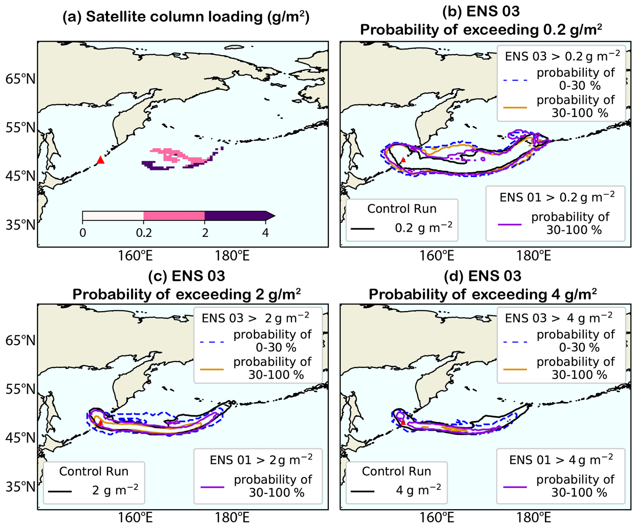
Figure C1 Same probability maps as in Fig. 7 in the main paper, with the addition of the 0 %–30 % probability region for ENS03 to exceed mass loading of (b) 0.2 g m⁻², (c) 2 g m⁻², and (d) 4 g m⁻² (dashed blue contours; the region within the blue line is a probability region up to 30 %).