Stratospheric ozone response to sulfate aerosol and solar dimming climate interventions based on the G6 Geoengineering Model Intercomparison Project (GeoMIP) simulations

This study assesses the impacts of stratospheric aerosol intervention (SAI) and solar dimming on stratospheric ozone based on the G6 Geoengineering Model Intercomparison Project (GeoMIP) experiments, called G6sulfur and G6solar. For G6sulfur, an enhanced stratospheric sulfate aerosol burden reflects some of the incoming solar radiation back into space to cool the surface climate, while for G6solar, the reduction in the global solar constant in the model achieves the same goal. Both experiments use the high emissions scenario of SSP5-8.5 as the baseline experiment and define surface temperature from the medium emission scenario of SSP2-4.5 as the target. In total, six Earth system models (ESMs) performed these experiments, and three out of the six models include interactive stratospheric chemistry. The increase in absorbing sulfate aerosols in the stratosphere results in a heating of the lower tropical stratospheric temperatures by between 5 to 13 K for the six different ESMs, leading to changes in stratospheric transport, water vapor, and other related changes. The increase in the aerosol burden also increases aerosol surface area density, which is important for heterogeneous chemical reactions. The resulting changes in the springtime Antarctic ozone between the G6sulfur and SSP5-8.5, based on the three models with interactive chemistry, include an initial reduction in total column ozone (TCO) of 10 DU (ranging between 0–30 DU for the three models) and up to 20 DU (between 10–40 DU) by the end of the century. The relatively small reduction in TCO for the multi-model mean in the first 2 decades results from variations in the required sulfur injections in the models and differences in the complexity of the chemistry schemes. In contrast, in the Northern Hemisphere (NH) high latitudes, no significant changes can be identified due to the large natural variability in the models, with little change in TCO by the end of the century. However, all three models with interactive chemistry consistently simulate an increase in TCO in the NH mid-latitudes up to 20 DU, compared to SSP5-8.5, in addition to the 20 DU increase resulting from increasing greenhouse gases between SSP2-4.5 and SSP5-8.5. In contrast to G6sulfur, G6solar does not significantly change stratospheric temperatures compared to the baseline simulation. Solar dimming results in little change in TCO compared to SSP5-8.5. Only in the tropics does G6solar result in an increase of TCO of up to 8 DU, compared to SSP2-4.5, which may counteract the projected reduction in SSP5-8.5. This work identifies differences in the response of SAI and solar dimming on ozone for three ESMs with interactive chemistry, which are partly due to the differences and shortcomings in the complexity of aerosol microphysics, chemistry, and the description of ozone photolysis. It also identifies that solar dimming, if viewed as an analog to SAI using a predominantly scattering aerosol, would succeed in reducing tropospheric and surface temperatures, but any stratospheric changes due to the high forcing greenhouse gas scenario, including the potential harmful increase in TCO beyond historical values, would prevail.

1 Introduction

There has been an increasing interest in researching climate intervention (CI) strategies because even ambitious mitigation efforts may not be sufficient to keep global mean temperature targets below 1.5 ^∘C above preindustrial levels, which is needed to prevent more serious climate impacts (IPCC, 2021). Furthermore, current commitments to reducing greenhouse gas emissions are falling way short of reaching the required temperature targets. Therefore, CI strategies beyond mitigation and adaptation may be the only way to prevent severe impacts on society and ecosystems. While research has been increasing in this direction, there is still considerable uncertainty on the effects of different proposed CI proposals on the climate system. One of the most studied solar radiation modification (SRM) approaches is the continuous injection of sulfur (SO₂) into the stratosphere, which results in an enhanced stratospheric aerosol burden that reflects some of the incoming sunlight to space and, therefore, cools the Earth's surface (NAS, 2021). This approach is called stratospheric aerosol intervention (SAI) in the following. An often-mentioned concern of SAI is the impact on stratospheric ozone, particularly the delay of the Antarctic ozone recovery (e.g., Tilmes et al., 2008; Heckendorn et al., 2009). The increase in stratospheric surface area density (SAD) from SAI is expected to impact heterogeneous chemical reactions similar to the observed impacts after large volcanic eruptions (e.g., Solomon, 1999). In addition, the heating of the lower tropical stratosphere from sulfate aerosols causes changes in stratospheric transport and circulation and an increase in stratospheric water vapor (e.g., Niemeier and Schmidt, 2017; Richter et al., 2017). Both these changes impact stratospheric ozone (e.g., Tilmes et al., 2017).

Recent studies investigated the impacts of SAI on stratospheric ozone with simulations using the Community Earth System Model (CESM) with the Whole Atmosphere Community Climate Model (WACCM) as the atmospheric component, a configuration denoted by CESM(WACCM). The experiments employed a high climate forcing future scenario (using Representative Concentration Pathway 8.5, RCP8.5, emissions) and required continuously increasing sulfur injections to keep surface temperatures at 2020 conditions (Tilmes et al., 2021). This study found that even a transient phase-in of sulfur injections can significantly deepen the ozone hole over Antarctica in October within the first 10 years of the application. Furthermore, the heating of the tropical lower stratosphere results in an increase in total column ozone in mid-to-high latitudes in the Northern Hemisphere winter (Richter et al., 2018; Tilmes et al., 2018). Another study analyzed the effects of SAI on ozone by using two different baseline scenarios, i.e., the Shared Socioeconomic Pathway (SSP) high forcing scenario SSP5-8.5 and the SSP5-3.4-OS scenario (Tilmes et al., 2020). SSP5-3.4-OS follows SSP5-8.5 until 2040 and afterwards assumes substantial decarbonization and active removal of CO₂ from the atmosphere, resulting in an overshoot (OS) of threshold temperatures defined by the Paris Agreement. SAI was applied in both scenarios to maintain temperatures below 1.5 or 2 ^∘C, with the latter allowing a phase-out of the sulfur injection once greenhouse gas (GHG) concentrations in the atmosphere started to decline in a so-called peak-shaving scenario (Wigley, 2006; Tilmes et al., 2016; MacMartin and Kravitz, 2016; IPCC, 2018)

The impact of SAI on ozone depends on the increase in SAD and aerosol mass that increases with the increasing SO₂ injection amount (Tilmes et al., 2020). A baseline scenario with higher climate forcings that requires much larger sulfur injections to reach the target surface temperatures by the end of the century resulted in a much stronger impact on ozone (both an increase and a decrease, depending on the region and season) than a scenario that would phase out injections towards the end of the 21st century. However, it is unclear how representative these recent studies are since they only used one modeling framework, namely CESM(WACCM).

The Geoengineering Model Intercomparison Project (GeoMIP) has defined a standardized set of model experiments to assess the effects of SRM methods, including SAI (Kravitz et al., 2011, 2015). Some of the earlier experiments include the injections of sulfur into the stratosphere, such as the G3 and G4 experiments (Pitari et al., 2014; Xia et al., 2017). These earlier modeling experiments used the Climate Model Intercomparison Project 5 (CMIP5) scenario RCP4.5. They considered either a constant equatorial injection of 5 Tg SO₂ yr⁻¹ between 2020 and 2070 (G4) or a progressively increasing injection of SO₂ to maintain temperatures at 2020 levels (G3). The injection altitude was different among models. Only four models included the required processes to simulate the impacts of SAI on ozone for the G4 experiment and two for the G3 experiment. Pitari et al. (2014) found a decline in stratospheric ozone in the polar regions with sulfur injections for all the participating models. However, the stratospheric aerosol distributions in those models presented considerable differences, making conclusions about the overall impacts of SAI on ozone hard to determine.

More recent GeoMIP experiments, G6sulfur and G6solar, defined for CMIP6 future emission pathways (SSPs), were designed to explore the effects of SAI and solar dimming in a more policy-relevant setting (Kravitz et al., 2015). Both experiments employ SSP5-8.5 as the baseline scenario. G6sulfur requires the application of sulfur injections between 10^∘ S–10^∘ N in latitude and around 18–20 km altitude to keep surface temperatures at the same values as those simulated in the SSP2-4.5 scenario for the 2020–2100 period (the target scenario). G6solar requires reducing the global solar constant to offset the same temperature difference to reach SSP2-4.5 values. The purpose of comparing both G6sulfur and G6solar is to identify the differences in those approaches, as past analyses have often described the reduction in the solar constant as a proxy for SAI (Ban-Weiss and Caldeira, 2010; Irvine et al., 2019). However, Niemeier et al. (2013) have shown that climate impacts, especially precipitation, differ between SAI and solar dimming. Visioni et al. (2021a) have shown that differences between these applications were identified regarding surface climate impacts and their effect on ozone, even if the solar dimming was applied to achieve the same global mean, inter-hemispheric, and pole-to-Equator surface temperature targets as SAI. Similarly, Xia et al. (2017) outlined the differences in the effects of solar dimming and SAI on stratospheric and tropospheric ozone. Both of these earlier studies used CESM(WACCM), while G6sulfur and G6solar experiments have been performed by six Earth system models (ESMs). Another proposal suggests using aerosols for SAI that absorb less solar radiation when integrated across the solar spectrum (Keith and Irvine, 2016; Dykema et al., 2016), which may reduce some of the climate impacts, including the precipitation reduction over southern Europe in winter (Jones et al., 2022) and weakening of the monsoonal precipitation over India (Simpson et al., 2019). Therefore, solar dimming may be a closer analog to SAI approaches using less absorbing aerosols than sulfates.

This study explores the impacts of SAI and global solar dimming on stratospheric ozone based on the G6sulfur and G6solar GeoMIP experiments. In total, the results of six ESMs that performed these GeoMIP experiments are available. However, only three different ESMs include comprehensive interactions between chemistry and aerosols in the stratosphere. Section 2 describes the details of the experimental design and models participating in this study. Results are described in Sect. 3 and include changes in stratospheric temperatures and transport and surface area distribution for both G6solar and G6sulfur and the effects on ozone concentration total column ozone (TCO) for selected regions and seasons. A summary is given in Sect. 4, and the discussion and conclusions are presented in Sect. 5.

2 Experimental design and model description

The GeoMIP G6solar and G6sulfur experiments use the SSP5-8.5 high greenhouse gas forcing scenario as their baseline scenario. SAI or global solar dimming are applied to reduce global surface temperatures to the levels derived for the SSP2-4.5 for each model. The experiment does therefore not aim towards reaching surface temperature targets of 1.5 ^∘C. The annual forcing required to achieve this goal in these experiments depends on the surface air temperature difference between SSP5-8.5 and SSP2-4.5. This difference strongly increases in the second half of the 21st century, with 0.19 ± 0.04 K global mean surface temperature differences in 2040 and 0.62 ± 0.05 K in 2060, 1.46 ± 0.14 K in 2080 and 2.42 ± 0.22 K in 2100, based on the GeoMIP multi-model mean in the participating models considering a 10-year running mean (Visioni et al., 2021b). According to these differences, the models required much less solar dimming or aerosol increase in the first half of the century than in the second half to reach the surface temperature of the target (SSP2-4.5) experiment.

Table 1 Summary of model simulations used in this work (adapted from Visioni et al., 2021b).

A total of six models participated in these experiments, as listed in Table 1 (adapted from Visioni et al., 2021b). The G6sulfur experiment required sulfur injections directly into the stratosphere. Only three models that performed G6 experiments include an interactive aerosol microphysical model in the stratosphere. Of these three models, two (IPSL-CM6A-LR and UKESM1-0-LL) injected SO₂ uniformly between 10^∘ N and 10^∘ S and 18 and 20 km of altitude at a single longitude (0^∘). These models used a distinct stepping of injections every 10 years. CESM2-WACCM6 injected SO₂ at the Equator at 25 km altitude. CESM2(WACCM) used a feedback control algorithm (MacMartin et al., 2017) to identify the injection amount required every year to reach the target surface temperatures. The other models used precalculated aerosol distributions to prescribe aerosol and optical properties, where a prescribed aerosol distribution was scaled to reach the required target temperature. CNRM-ESM2-1 used an input dataset provided by GeoMIP (from the G4SSA experiment; Tilmes et al., 2015), while MPI-ESM prescribed their aerosol distribution derived from the aerosol microphysical simulations described in Niemeier and Schmidt (2017) and Niemeier et al. (2020).

Only three out of the six coupled Earth system models, UKESM1-0-LL, CESM2(WACCM), and CNRM-ESM2-1 included interactive stratospheric chemistry, including ozone and water vapor coupled to the radiation scheme, which is required to determine the impacts of SAI on ozone. Only two out of the three models, UKESM1-0-LL and CESM2(WACCM), include interactive aerosol microphysical schemes. The other three models used prescribed ozone fields, which differed only between SSP5-8.5 and SSP2-4.5 (Keeble et al., 2021). The CNRM-ESM2-1 chemistry scheme considers 168 chemical reactions, among which 39 are photolysis reactions, and 9 reactions that represent heterogeneous chemistry. This scheme is applied above 560 hPa but does not include non-methane hydrocarbon chemistry in the calculation of tropospheric ozone. The model does not include an interactive aerosol microphysical model in the stratosphere and uses a prescribed stratospheric aerosol distribution. The photolytic calculation considers changes in the chemical composition but does not consider changes in aerosols. A full description and evaluation of CNRM-ESM2-1 can be found in Séférian et al. (2019). The evaluation of the ozone radiative forcing is described in Michou et al. (2020).

The UKESM1-0-LL model uses a combined stratospheric–tropospheric chemistry scheme (Archibald et al., 2020) including 84 tracers, 199 bimolecular reactions, 25 unimolecular and termolecular reactions, 59 photolytic reactions, 5 heterogeneous reactions, and 3 aqueous-phase reactions for the sulfur cycle from the United Kingdom Chemistry and Aerosols (UKCA) model. Although an extended stratospheric chemistry scheme is available that includes the explicit treatment of most of the long-lived ozone-depleting substances ODSs of importance for the recovery of stratospheric ozone and that participated in the Chemistry Climate Model Initiative (CCMI; e.g., Dhomse et al., 2018), this scheme was not used in UKESM1-0-LL. Instead, the lower boundary conditions of halogenated ODSs are lumped into three main halogenated source gases (CFC11, CFC12 and CH3Br). UKESM1-0-LL uses the UKCA Global Model of Aerosol Processes (UKCA-GLOMAP) modal aerosol scheme (Mann et al., 2010) and interactive Fast-JX photolysis scheme, which is applied to derive photolysis rates between 177 and 850 nm, as described in Telford et al. (2013). In the lower mesosphere, photolysis rates are calculated using lookup tables (Lary and Pyle, 1991). The performance of UKESM1-0-LL is described in detail in Sellar et al. (2019).

CESM2-WACCM6 uses the Whole Atmosphere Community Climate Model, version 6 (WACCM6), as its atmosphere component. The model includes comprehensive chemistry in the troposphere, stratosphere, mesosphere, and lower thermosphere (TSMLT), including 231 species, 150 photolysis reactions, 403 gas-phase reactions, 13 tropospheric heterogeneous reactions, and 17 stratospheric heterogeneous reactions (Emmons et al., 2020). The photolytic calculations use both inline chemical modules and a lookup table approach, which does not consider changes in aerosols. CESM2-WACCM6 includes a prognostic representation of stratospheric aerosols based on sulfur emissions from volcanoes and other sources (Mills et al., 2017). The performance of CESM2-WACCM6 is described in detail in Gettelman et al. (2019).

The three models described above all participated in the CMIP6, and evaluations of stratospheric ozone and water vapor showed generally good agreement with observations but a few notable differences (Keeble et al., 2021). In comparison to observations and the multi-model mean, UKESM1-0-LL significantly overestimated the total column ozone globally. This behavior was partially related to the limited treatment of heterogeneous chlorine and bromine chemistry. The model produces a more negative trend in high latitudes than observed between 1960 and 2014. CNRM-ESM2-1 underestimates TCO in the polar regions while overestimating TCO in the tropics but shows a reasonable decline in ozone between 1960 and 2014 (Séférian et al., 2019). CESM2-WACCM6 TCO is in good agreement with observations but underestimates the negative trend between 1960 and 2014 in the Northern Hemisphere high latitudes. In the following analyses, we show TCO model results relative to 2020 conditions to remove model biases in TCO.

In addition to differences in chemistry, different radiative schemes contribute to differences in aerosol heating in G6sulfur. The UK model uses the SOCRATES (https://code.metoffice.gov.uk/trac/socrates, last access: 4 April 2019) radiative transfer scheme (Edwards and Slingo, 1996; Manners et al., 2015) with a new configuration for the Met Office Unified Model Global Atmosphere version 7.0 (Walters et al., 2019). The MPI models use the radiation scheme by Pincus and Stevens (2013) and Mauritsen et al. (2019). This radiation scheme is a modification of the Rapid Radiation Transfer Model (RRTM). Both CNRM-ESM2-1 and IPSL-CM6A-LR use an updated version of the Fouquart–Morcrette scheme (Fouquart and Bonnel, 1980; Morcrette et al., 2008), with six bands for the short-wave radiation and 16 bands of the RRTM scheme (Mlawer et al., 1997) for the long-wave radiation. Finally, CESM2-WACCM uses RRTM for both long-wave and short-wave radiation.

3 Results

Overall changes in stratospheric ozone concentration are due to a combination of the following different factors: dynamical changes resulting in transport differences, changes in heterogeneous chemistry induced by larger SAD values, and temperature- and photolysis-driving differences in reaction rates (Pitari et al., 2014; Tilmes et al., 2018; Visioni et al., 2021a), as outlined in this section.

3.1 Effects of SAI and solar dimming on atmospheric temperature and winds

In G6sulfur and G6solar, SAI and solar dimming have been applied to the SSP5-8.5 baseline scenario to reach global mean surface temperatures simulated for the target scenario SSP2-4.5. To understand the stratospheric changes from the G6 application, we first discuss the changes between the baseline and the target scenario. The increase in greenhouse gases results in an increase in tropospheric temperatures and cooling of the stratosphere (Fels et al., 1980; Pisoft et al., 2021). This will introduce changes in the meridional gradient of the zonal mean temperature, which, by geostrophic balance, implies changes in zonal mean wind. Changes in the zonal wind, especially near the top and equatorward flanks of the tropospheric jets, then affect wave forcing and with that the shallow branch of the Brewer–Dobson circulation (BDC) (Shepherd and McLandress, 2011). In addition, changes in the tropical upwelling and a strengthening of the polar vortex can be inferred for the three models between SSP2-4.5 and SSP5-8.5 which are, however, not significant (Fig. A1; middle panels).

Figure 1 Zonal mean temperature changes (2080–2099) between G6sulfur and SSP5-8.5 for all GeoMIP models participating in the G6 experiment. Contour lines show the baseline SSP5-8.5 temperature. Gray horizontal lines indicate changes that are not statistically significant over the time period considered when using a double-sided t test at 95 % confidence levels.

G6sulfur and G6solar act in addition to the changes caused by greenhouse gases. The increase in aerosol optical depth (AOD) and solar dimming successfully counteracts the temperature increase in the troposphere and at the global surface between SSP2-4.5 and SSP5-8.5 for all the models (Visioni et al., 2021b). The cooling of the stratosphere due to the high greenhouse gas concentrations prevails for G6solar. For G6sulfur, the increased stratospheric sulfate burden with increasing sulfur injections cause the warming of the lower tropical stratosphere compared to the baseline experiment SSP5-8.5 (Fig. 1) and compared to SSP2-4.5 (Fig. A2).

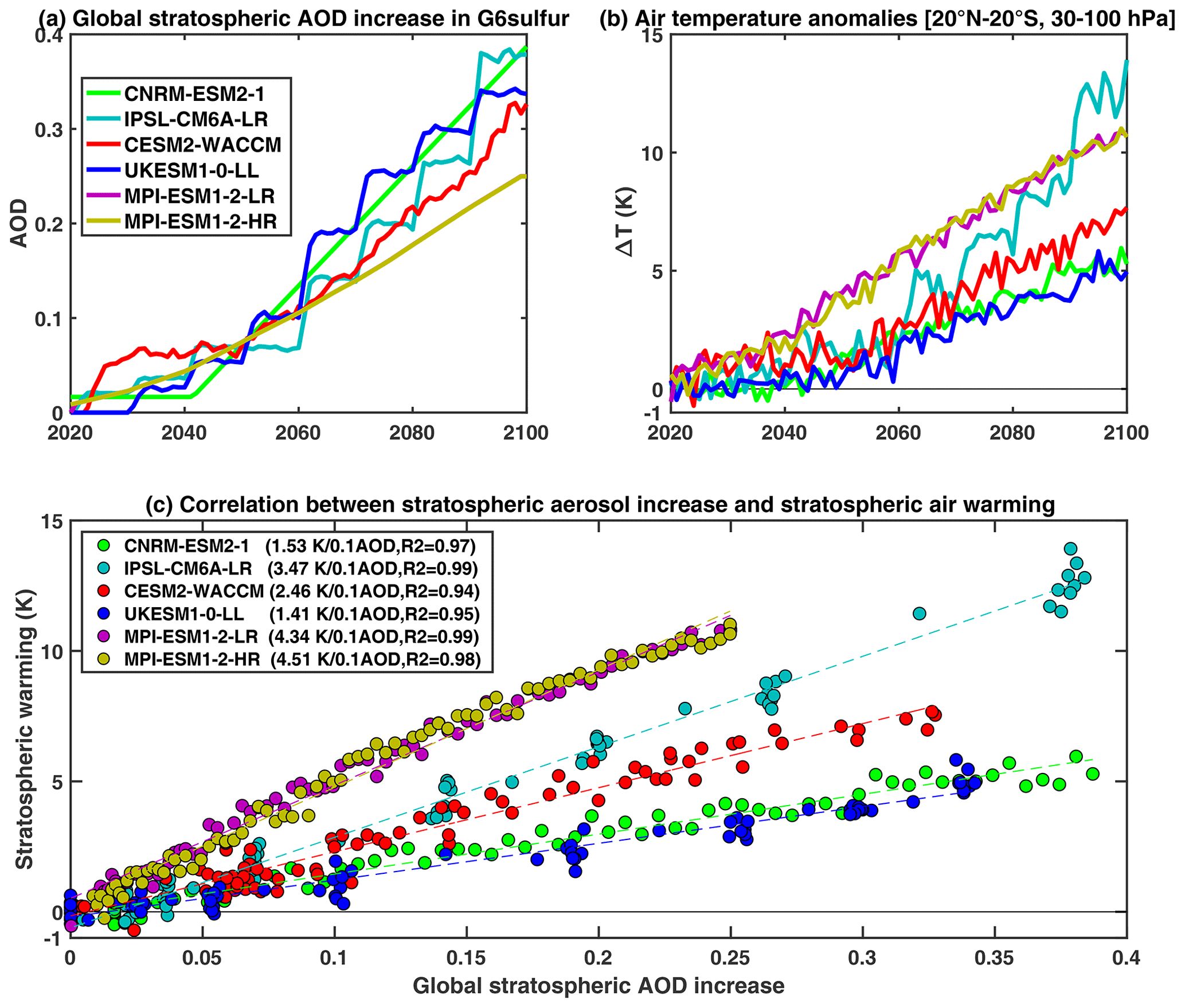
Figure 2 (a) Evolution of the global mean increase in stratospheric aerosol optical depth for each model in G6sulfur. (b) Evolution of the yearly mean stratospheric temperatures (20^∘ N–20^∘ S; 30–100 hPa) for each model in G6sulfur. (c) Correlation between values in panels (a) and (b) with the slope of the fitted linear function and the correlation coefficient (R²). Both MPI-ESM1-2-LR and MPI-ESM1-2-HR use the same described aerosol distribution.

Models differ substantially in the amount of stratospheric heating in G6sulfur by the end of the experiment (2080–2099) (Fig. 2). As pointed out in Visioni et al. (2021b), variations in the heating response to sulfates in the models can be caused by different quantities, including aerosol mass and aerosol size distribution, differences in the heating rates as the result of the different radiative schemes, stratospheric chemical composition, and water vapor. Differences in the radiation scheme play an important role (Neely and Schmidt, 2016) for both long- and short-wave radiation (Niemeier et al., 2020). While the schemes substantially differ for the MPI-ESM1-2 models and UKESM1-0-LL, CNRM-ESM2-1, IPSL-CM6A-LR, and CESM2-WACCM all use the same radiative schemes for the long-wave radiation (see Sect. 3). However, even when using a similar radiative scheme in the long wave, these three models show differences in the heating response (Fig. 2c), which is, in part, a result of differences in the amount and distribution of aerosol mass. For example, CESM2-WACCM6 heating extends toward higher altitudes because injections were performed at higher altitudes than in the other models. Other differences include using a prescribed aerosol distribution with fixed aerosol sizes that do not increase with an increasing injection amount (CNRM-ESM2-1) compared to interactive aerosol schemes.

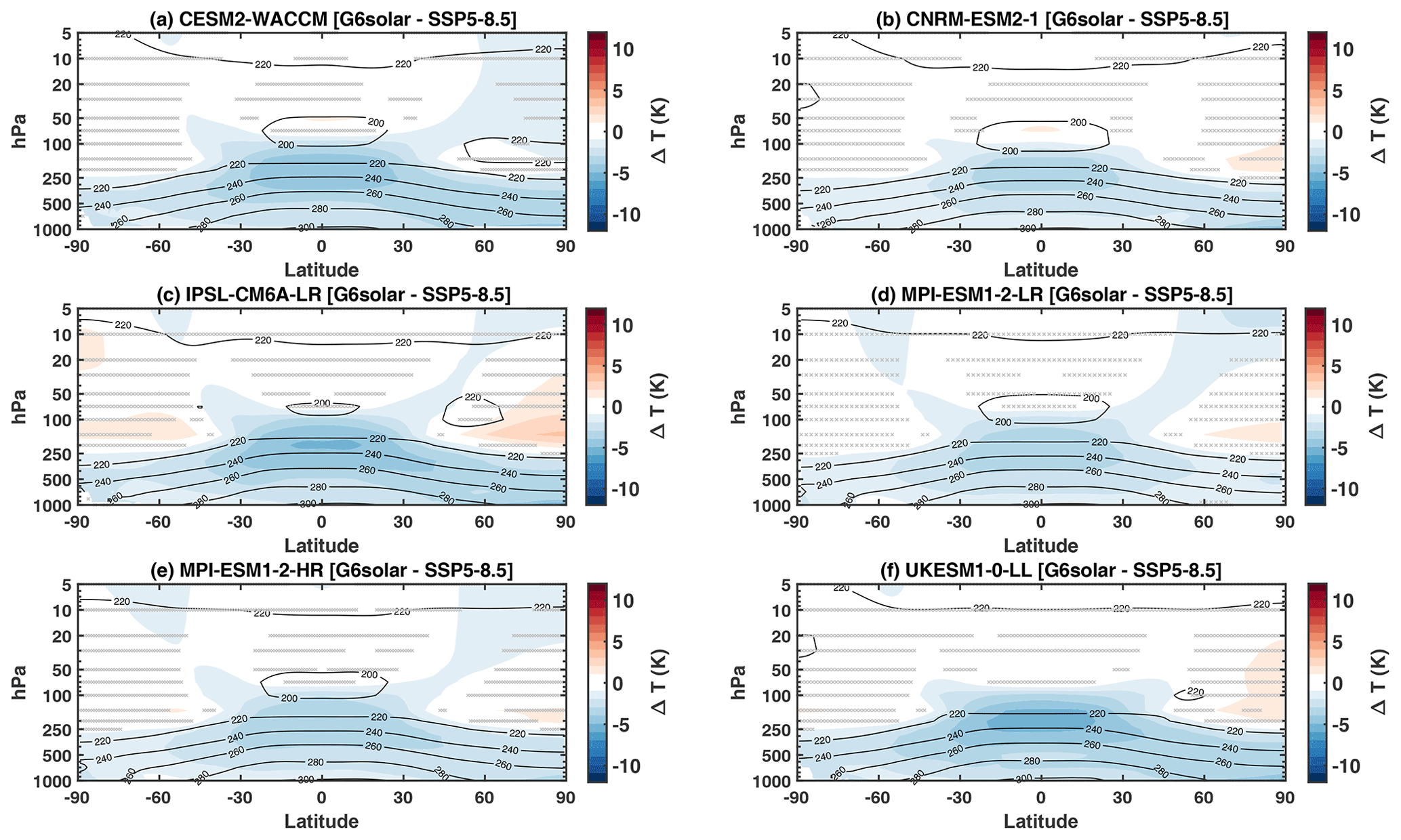
Figure 3 Zonal mean temperature changes (2080–2099) between G6solar and SSP5-8.5 for all GeoMIP models participating in the G6 experiment. Contour lines show the baseline SSP5-8.5 temperature. Gray horizontal lines indicate changes that are not statistically significant over the time period considered when using a double-sided t test at 95 % confidence levels.

Another important difference between all six models is the use of prescribed vs. interactive chemistry. Richter et al. (2017) have shown that stratospheric aerosol injection experiments produce more tropical stratospheric heating if the simulation uses prescribed chemistry rather than interactive chemistry. The temperature increase between 30 and 100 hPa and 20^∘ N–20^∘ S reaches between 5 and 13 K for the six different models (Fig. 2c). However, if we only consider the three models with interactive chemistry (as used in the following analysis), i.e., CNRM-ESM2-1 (with a prescribed aerosol distribution) and UKESM1-0-LL and CESM2-WACCM6 (with interactive aerosols), then these models show a smaller range of temperature increase, between 5 and 7 K, by the end of the century, which is consistent with what has been shown in Richter et al. (2017). More specific model experiments will be needed to quantify the contributions of the different factors that lead to differences in the radiative heating. In contrast to G6sulfur, solar dimming in G6solar does not lead to a significant temperature change in the stratosphere compared to SSP5-8.5 (Fig. 3), and stratospheric temperatures stay lower compared to SSP2-4.5. As per the experimental design, the solar dimming in both experiments leads to a similar surface cooling.

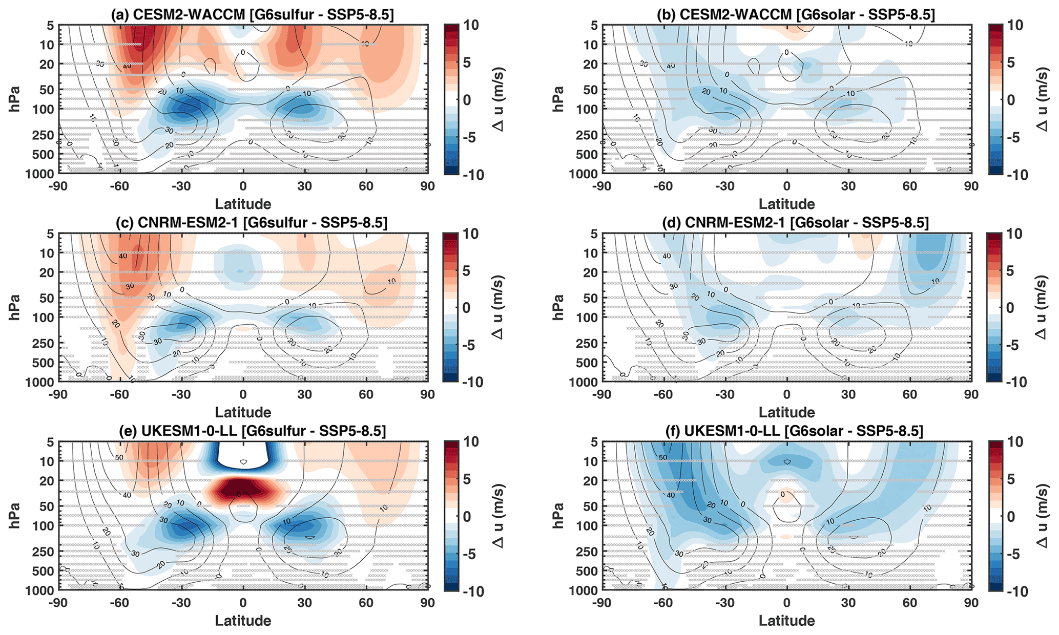
Figure 4 Zonal mean zonal wind changes (m s⁻¹) (2080–2089) between G6sulfur and SSP5-8.5 (a, c, e) and G6solar and SSP5-8.5 (b, d, f) for the three GeoMIP models with interactive chemistry that participated in the G6 experiment. Contour lines show the baseline SSP5-8.5 winds. Gray horizontal lines indicate changes that are not statistically significant over the period considered when using a double-sided t test at 95 % confidence levels.

The cooling of the troposphere with solar dimming in G6solar results in a slowing of the BDC and weakening of the subtropical jet stream (STJ) and the polar vortex compared to SSP5-8.5 (Fig. 4; right column). This experiment therefore successfully reverses the effect of increasing greenhouse gases between SSP2-4.5 and SSP5-8.5 by the end of the century (Fig. A1; right column). On the other hand, significant zonal wind changes by the end of the century occur for G6sulfur (Fig. 4; left column) for all three models, including a weakening of the subtropical jet stream and a strengthening of the polar vortex compared to SSP5-8.5, consistent with what has been found in early studies (e.g., Tilmes et al., 2017; Jones et al., 2022).

Changes in the tropical upwelling, illustrated by the vertical wind component (w^∗) derived from the transformed Eulerian mean (TEM) stream function, depend on the details of the experiment (Fig. 5). Only WACCM6 results are analyzed due to the lack of available information for the other models. For G6sulfur, the weakening of the subtropical storm tracks is aligned with reduced vertical wind velocity around the tropopause and below the injection altitude. Interestingly, the reduction in w^∗ overcompensates the conditions for the target simulation and results in values similar to present-day conditions. Above the sulfur injection location, w^∗ is increased compared to SSP5-8.5. In contrast, w^∗ in G6solar matches the target scenario SSP2-4.5.

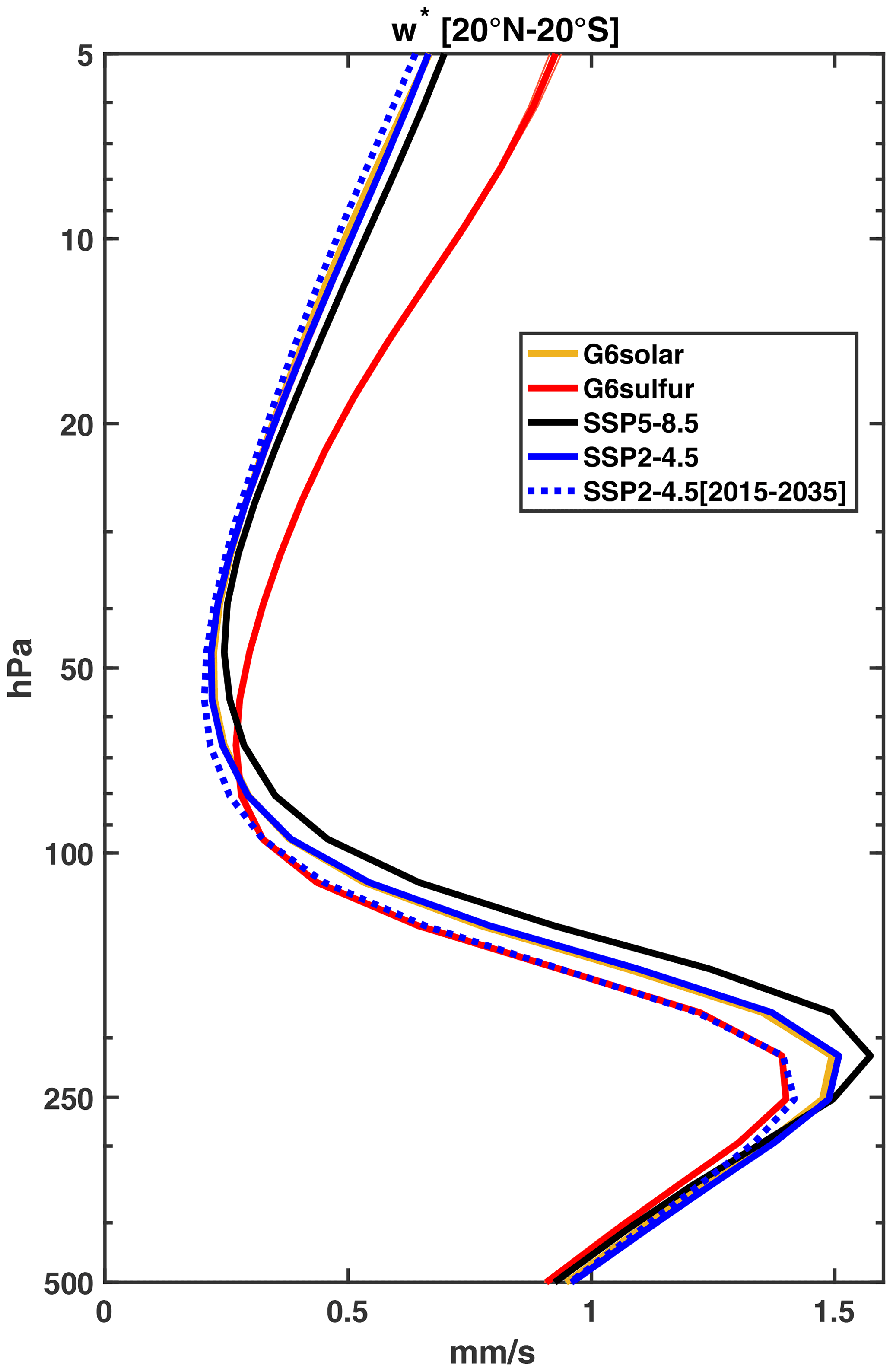
Figure 5 Zonally and annually averaged residual vertical velocity (w^∗), averaged between 30^∘ N and 30^∘ S, for CESM2-WACCM6 for 2080–2100 and for different experiments (colored solid lines) and for 2015–2035 for SSP2-4.5 (blue dotted lines).

Besides the commonalities among the three models, some differences exist. For the G6sulfur experiments, the three models differ in their response in zonal wind between 50 and 5 hPa (Fig. 4). WACCM6 shows a strengthening of the tropical winds, and CNRM-ESM2-1 shows a weakening of the tropical winds. UKESM1-0-LL shows a strong increase in the zonal tropical winds between 20–50 hPa and a decrease above those altitudes by the end of the century, which is aligned with the permanent lock-in of the quasi-biennial oscillation (QBO) into a westerly phase after 2055 (Jones et al., 2022). These differences are likely connected to the differences in the heating response that are caused by different injection strategies, with injections in lower altitudes showing stronger heating and change in w^∗ than injections in higher altitudes (Tilmes et al., 2017).

Furthermore, some non-significant differences in the model results for both G6sulfur and G6solar compared to the baseline are obvious in the first 20 years of the application (Fig. A3). CNRM-ESM2-1 shows a weakening of the polar vortex in the Southern Hemisphere for G6sulfur and a strengthening of the polar vortex in both hemispheres in G6solar compared to the baseline simulation. This, however, is not related to the solar or sulfur applications because injections in this model had not ramped up before 2040 (see below) and, therefore, is a result of internal variability.

3.2 Effects of SAI on surface area density

The three ESMs with interactive chemistry applied different strategies to counteract the warming between SSP5-8.5 and SSP2-4.5 with stratospheric aerosols (see Sect. 2). Resulting differences in the changes in SAD, as described in this section (Fig. 6), have different impacts on heterogeneous chemistry and, therefore, ozone in the stratosphere.

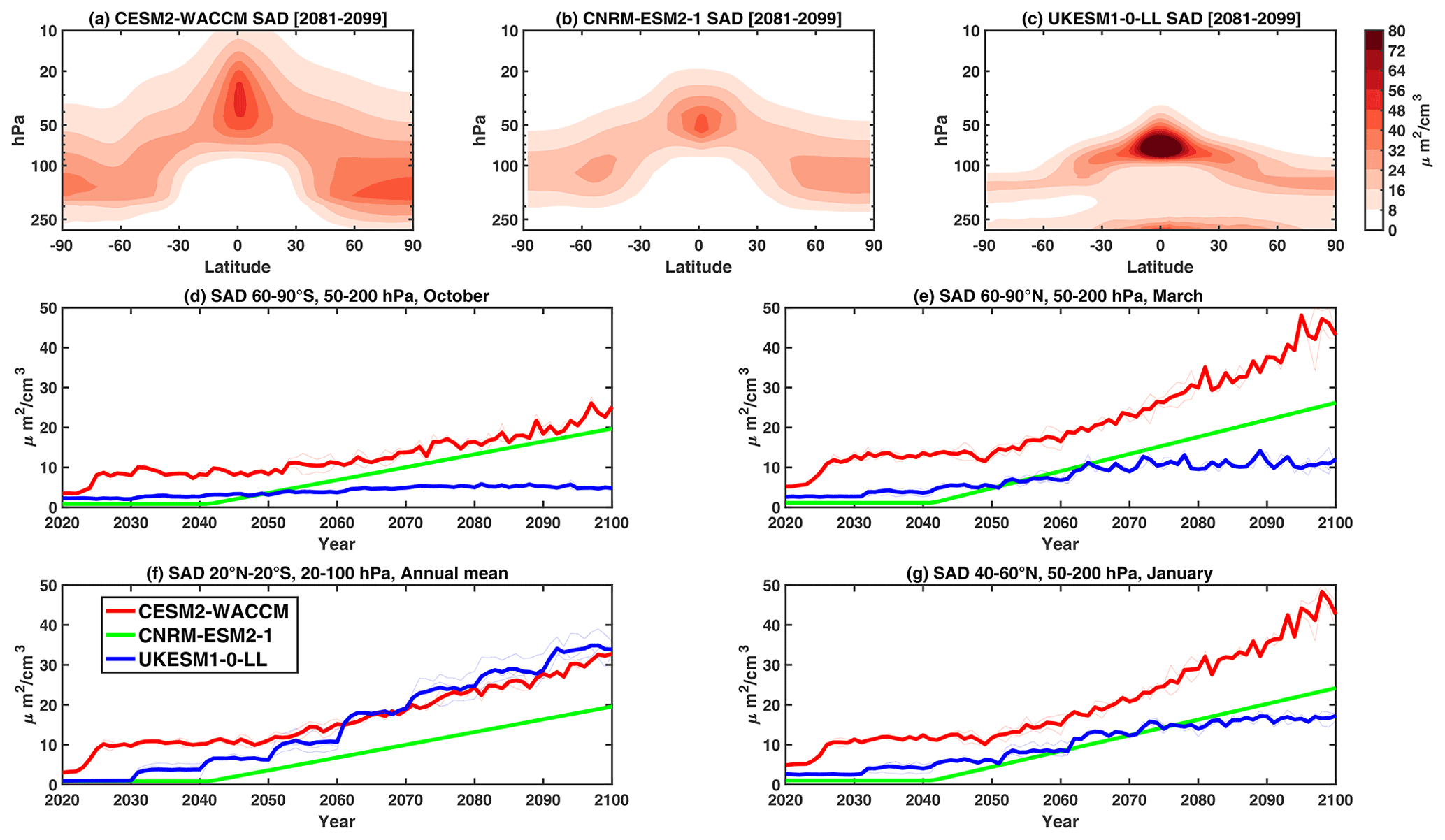
Figure 6 (a–c) Aerosol surface area density (SAD; µm² cm⁻³) for the three models with interactive stratospheric chemistry in the 2081–2099 period. (d–g) Temporal evolution of SAD for the three models over the whole simulation period for different locations and times of the year, with (d) 60–90^∘ S in October, (e) 20^∘ N–20^∘ S for the annual mean, (f) 40–60^∘ N in January, and (g) 60–90^∘ N in March.

As described in Sect. 2, CESM2-WACCM6 injected sulfur at 25 km (≈ 30 hPa). This resulted in an aerosol distribution that covers a larger altitude range compared to that of other models. Furthermore, the experiment required an initial increase of sulfur emissions of around 2 Tg SO₂ yr⁻¹ in the first 3 years of the start of the application, which stayed at around 2–3 Tg SO₂ yr⁻¹ emissions until 2045 (as shown in Visioni et al., 2021b). This relatively small injection amount results in a sudden increase in SAD from 2 to 10 µm² cm⁻³ within the first year of the application (Fig. 6). This happens because the aerosol microphysical scheme first produces smaller particles that grow slowly with increasing injection, resulting in the initial increase in SAD (as also discussed in Tilmes et al., 2021). After this initial increase, SAD and AOD (Fig. 2a) stay constant until about 2050, along with the roughly constant injection amount. After 2050, increased sulfur emissions required to counteract the increasing warming resulted in a moderate increase in SAD in the tropics (Fig. 6f). The increase in SAD differs among regions and seasons. In winter and spring, the Northern Hemisphere (NH) mid- and high latitudes see a stronger increase in SAD than the Southern Hemisphere (SH) polar regions and the tropics (Fig. 6). A possible reason is the increased meridional transport of air and aerosols towards the NH mid- and high latitudes with SAI applications, which can be caused by the weakening of the subtropical jet stream that reduces the subtropical wave forcing and, therefore, decelerates the shallow branch of the BDC.

UKESM1-0-LL injected sulfur in 18–20 km and between 10^∘ N–10^∘ S, as originally specified by the G6sulfur protocol in Kravitz et al. (2015). The resulting aerosol distribution is nonetheless constrained in a small region above the tropopause, leading to a large peak in SAD (above 70 µm² cm⁻³) between 10^∘ N–10^∘ S and between 100–50 hPa by the end of the century and smaller SAD outside that region compared to the other models (Fig. 6c). Sulfur emissions for G6sulfur started in 2030 and ramped up every 10 years with a small increase until 2050 and accelerated increases after that. After 2050 SAD a similar trend in the tropics, to that in CESM2-WACCM6, follows (Fig. 6f). However, the initial strong increase in SAD found in CESM2-WACCM6 does not occur in UKESM1-0-LL. This could be a result of the production of larger aerosol particles (and therefore smaller SAD) in UKESM1-0-LL compared to CESM2-WACCM6 for the same injection amount because of stronger vertical transport in CESM2-WACCM and a stronger confinement of the enhanced aerosol distribution in UKESM1-0-LL. Long-term increases in SAD are similar to CESM2-WACCM6 in the tropics after 2040, but much lower than the other two models in high latitudes, particularly in the SH.

CNRM-ESM2-1 uses a prescribed stratospheric aerosol distribution that is scaled depending on the requirement to offset the warming between SSP2-4.5 and SSP5-8.5. The aerosol and SAD distribution are generally similar to WACCM6 but smaller and slightly less spread out by the end of the century (Fig. 6b). CNRM-ESM2-1 does not apply SAI until after 2040 and applies a linear increase with time after that date mainly because the difference in surface air temperature between SSP8-8.5 and SSP2-4.5 cannot be disentangled from the model internal variability before 2040 (Visioni et al., 2021b). We find a linear increase with time in SAD because of the scaled, fixed aerosol distribution that does not consider potential changes in the aerosol size distribution with injection amount or changes in the spatial distribution of the aerosol from transport. The resulting SAD is smaller (by almost half) in the tropics compared to the other two models. A similar but slightly smaller increase after 2060 is found in the SH high latitudes in October, half the increase in SAD in the NH high latitudes in March, and a similar SAD in NH mid-latitudes in January compared to UKESM1-0-LL.

3.3 Effects of SAI and solar dimming on ozone concentration

As for the temperature response, first we briefly outline differences in ozone mixing ratios between SSP2-4.5 and SSP5-8.5 (Fig. A4). The increasing acceleration of the BDC (Sect. 3.1) results in ozone reduction around the tropical tropopause due to the increased transport of ozone-poor air masses into the lower tropical stratosphere. In addition, the cooling of the stratosphere results in a slowing of temperature-dependent catalytic ozone loss reactions, which causes an increase in ozone under colder stratospheric conditions (Haigh and Pyle, 1982), as further outlined in Nowack et al. (2016).

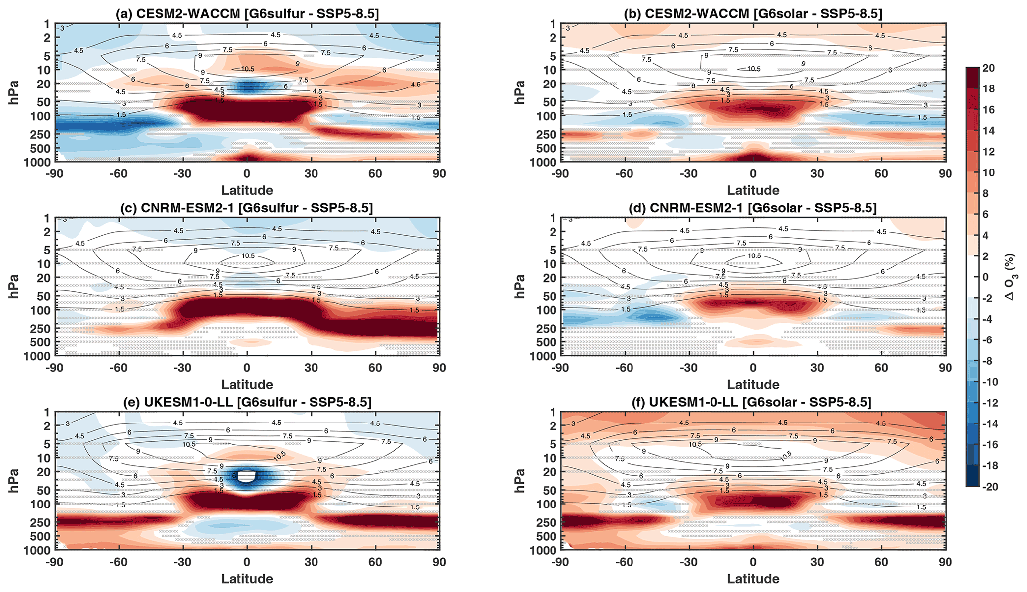
Figure 7 Ozone concentration changes (in percent of SSP5-8.5) for the G6sulfur (a, c, e) and G6solar (b, d, f) cases compared to SSP5-8.5 in the 2080–2099 period. Contour lines show the baseline SSP5-8.5 ozone concentration over the same period. Gray horizontal lines indicate changes that are not statistically significant over the period considered when using a double-sided t test at 95 % confidence levels.

Solar dimming reverses the acceleration of the BDC for G6solar. This results in an increase in ozone in the lower tropical stratosphere and a decrease in the upper troposphere and lower stratosphere (UTLS) at mid- and high latitudes (for WACCM6 and CNRM-ESM-1), as also found in Nowack et al. (2016) and Xia et al. (2017). However, solar dimming does not reverse the increase (super recovery) in ozone in all of the stratosphere. In contrast, it can result in a further ozone increase in the upper stratosphere compared to the baseline scenario, as is most apparent in UKESM1-0-LL (Fig. 7; lower right panel). As explained in Nowack et al. (2016), this is based on two main drivers. First, the reduced insolation in G6solar results in less ozone photolysis and less abundant atomic oxygen and, with that, a slowing of catalytic ozone loss reactions and, second, a significant reduction in stratospheric humidity produced by the tropospheric cooling reduces ozone loss via odd hydrogen catalytic cycles. This increase in stratospheric ozone compared to the baseline simulations further impacts ozone in the UTLS and the troposphere through the exchange of air masses from the stratosphere to the troposphere. The increase in ozone in the UTLS further results in a decrease in oxygen photolysis and, therefore, an increase in tropospheric ozone.

G6sulfur simulations show a much more substantial increase in ozone right above the tropical tropopause than G6solar for all the models. In addition, results show a reduction in ozone between 50 and 20 hPa and an increase at about 10 hPa for WACCM6 and UKESM1-0-LL as a result of changes in w^∗ (Fig. 5), as also shown in the earlier studies discussed above. In addition to the dynamical changes, the increase in SAD results in a reduction in the NO_x chemical cycle and an increase in ozone. The increase in ozone of around 5–10 hPa is strongest in CESM2-WACCM6, consistent with the largest increase in SAD in that region. This is also consistent with the largest increase in ozone above 50 hPa in mid- and high latitudes by the end of the century in CESM2-WACCM6. In addition, reductions in shortwave radiation as the result of the ozone increase can result in an inverse self-healing of ozone below (Nowack et al., 2016; Pitari et al., 2014) and, therefore, a reduction in ozone for both G6sulfur and G6solar, which likely contributes to the reductions in ozone in the tropics of around 20 hPa and in the troposphere for both WACCM6 and UKESM1-0-LL.

A reduction in the strength of the subtropical jet (Fig. 4), which is much more pronounced in G6sulfur than in G6solar, is expected to impact the meridional transport of ozone from the tropics to the mid- and high latitudes (as discussed above). The much stronger increase in ozone in the mid- to high latitudes in the UTLS for G6sulfur compared to G6solar (Fig. 7) is aligned with a stronger meridional transport and is most obvious for CNRM-ESM2-1 and UKESM1-0-LL. Ozone depletion in high polar latitudes as a result of increased SAD is most obvious in CESM2-WACCM6 (Fig. 7; top panels). As discussed above, smaller SAD in the other models does result in less ozone depletion in these regions. In the case of UKESM1-0-LL, heterogeneous activation of halogens on sulfate aerosols does not include any bromine reactions or the important hydrogen chloride plus chlorine nitrate reaction.

Changes in ozone in the UTLS further impacts ozone in the troposphere through vertical transport, as also discussed in Xia et al. (2017). WACCM6 shows a reduction in ozone in the lowermost stratosphere (below about 100 hPa) for mid- and high latitudes driven by ozone depletion in the polar lower stratosphere. In contrast, the increase in ozone in the stratosphere likely contributes to the increase in ozone in the UTLS for UKESM1-0-LL and CNRM-ESM2-1. In addition, tropospheric ozone is impacted by changes in the photochemistry in both G6sulfur and G6solar, as outlined in detail in Nowack et al. (2016) and Xia et al. (2017). An increase in tropospheric ozone results from decreased chemical ozone loss due to reduced tropical humidity, resulting from the relative cooling of the surface.

Finally, a change in the O₂ photolysis rate and UV-B radiation due to changes in ozone and aerosols impacts tropospheric ozone. Reductions in the column ozone and the resulting increase in UV-B in high latitudes are partly offset by the reduction in UV-B from the aerosol layer (e.g., Tilmes et al., 2012; Pitari et al., 2014). In this study, UKESM1-0-LL is the only model that includes an interactive photolysis scheme that takes the effects of aerosols into account, while all the models include changes due to ozone. The increase in aerosol burden and the resulting reduction in oxygen photolysis likely contributes to the increase in tropospheric ozone in UKESM1-0-LL.

3.4 Effects of SAI and solar dimming on total column ozone (TCO)

Total column ozone in SSP5-8.5 and SSP2-4.5 increases in the mid- and high latitudes between 2020 and 2100 and reaches above 1960 values for high greenhouse gas forcing scenarios due to the slow reduction in stratospheric halogen loading as the result of the Montreal Protocol (WMO, 2018; Keeble et al., 2021). In addition, enhanced greenhouse gases cool the stratosphere and, in turn, slow down ozone-destroying reactions, resulting in an increase in ozone. In addition, a warmer troposphere drives the acceleration of the BDC and concomitant changes in the stratospheric lifetime of tracers, including ozone (WMO, 2018). On the other hand, in the tropics, high forcing scenarios show an initial increase, and later a decrease, in TCO, consistent with an acceleration of the BDC and a decrease in the tropical lower stratospheric ozone (e.g., Meul et al., 2016; Keeble et al., 2017).

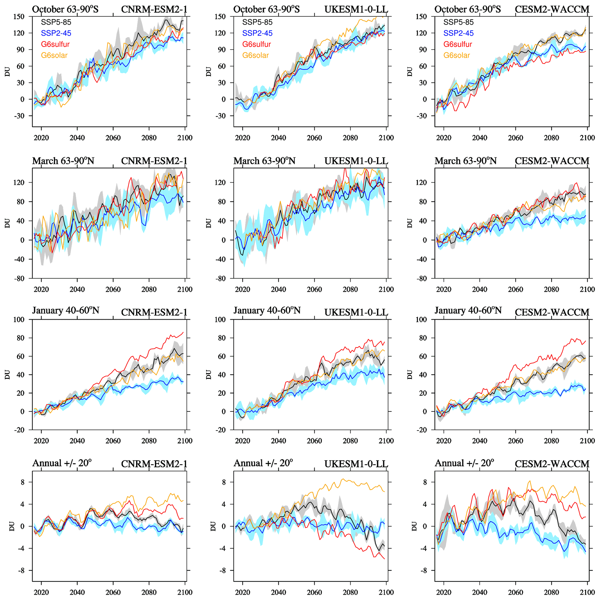
Figure 8 Ensemble mean of the total column ozone evolution between 2020 and 2100 normalized to 2020 values for different experiments (different colors) and four different regions and seasons (different rows) and three models (different columns). The 2σ standard deviation of the ensemble mean is only shown for SSP5-8.5 and SSP2-4.5 scenarios for better readability.

The three GeoMIP models follow the general behavior outlined above; however, specific differences exist (Fig. 8; black and blue lines). Both WACCM6 and CNRM-ESM2-1 show a stronger recovery in SSP5-8.5 than in SSP2-4.5 for spring in high polar latitudes, which agrees with the multi-model mean derived in Keeble et al. (2021). While UKESM1-0-LL does not show significant changes in TCO between these two forcing scenarios, this version of the model does not explicitly treat most of the long-lived ODS important for the ozone recovery (see Sect. 2), which could contribute to this behavior. On the other hand, WACCM6 does not show a very strong recovery in the NH high polar regions because of a warm bias in the model in this region which did not properly reproduce the reduction of ozone between 1980–2000 (Gettelman et al., 2019).

3.4.1 Effects of SAI on TCO

In the SH polar region in October, for G6sulfur compared to SSP5-8.5 (Fig. 9), WACCM6 shows a significant decline in TCO up to 30 DU for the ensemble mean at the start of the sulfur injection in 2020. After that, TCO declines much slower, towards 38 DU, by the end of the century. The changes are aligned with changes in SAD (Fig. 6d), since chemical changes strongly control the ozone in this region, and the slow decline in stratospheric halogen content, resulting in reduced chemical ozone loss. CNRM-ESM2-1 simulates decreasing TCO between 2040 and 2100, which is also aligned with the increase in SAD and is smaller than what is simulated in CESM2-WACCM6. However, due to the linear increase in SAD, CMRM-ESM2-1 does not show a strong decrease in ozone during the onset of the SAI application. UKESM1-0-LL shows much smaller reductions in TCO in the SH polar region than the other models due to a smaller increase in SAD. Because of differences in timing and magnitude of SAD changes, there is a large spread in the TCO response between the three models in this region. The ensemble mean shows an initial decrease in TCO of 10 DU ozone loss and closer to 20 DU by the end of the century (Fig. 11). Compared to SSP2-4.5, there is no significant change in TCO, besides the initial reduction.

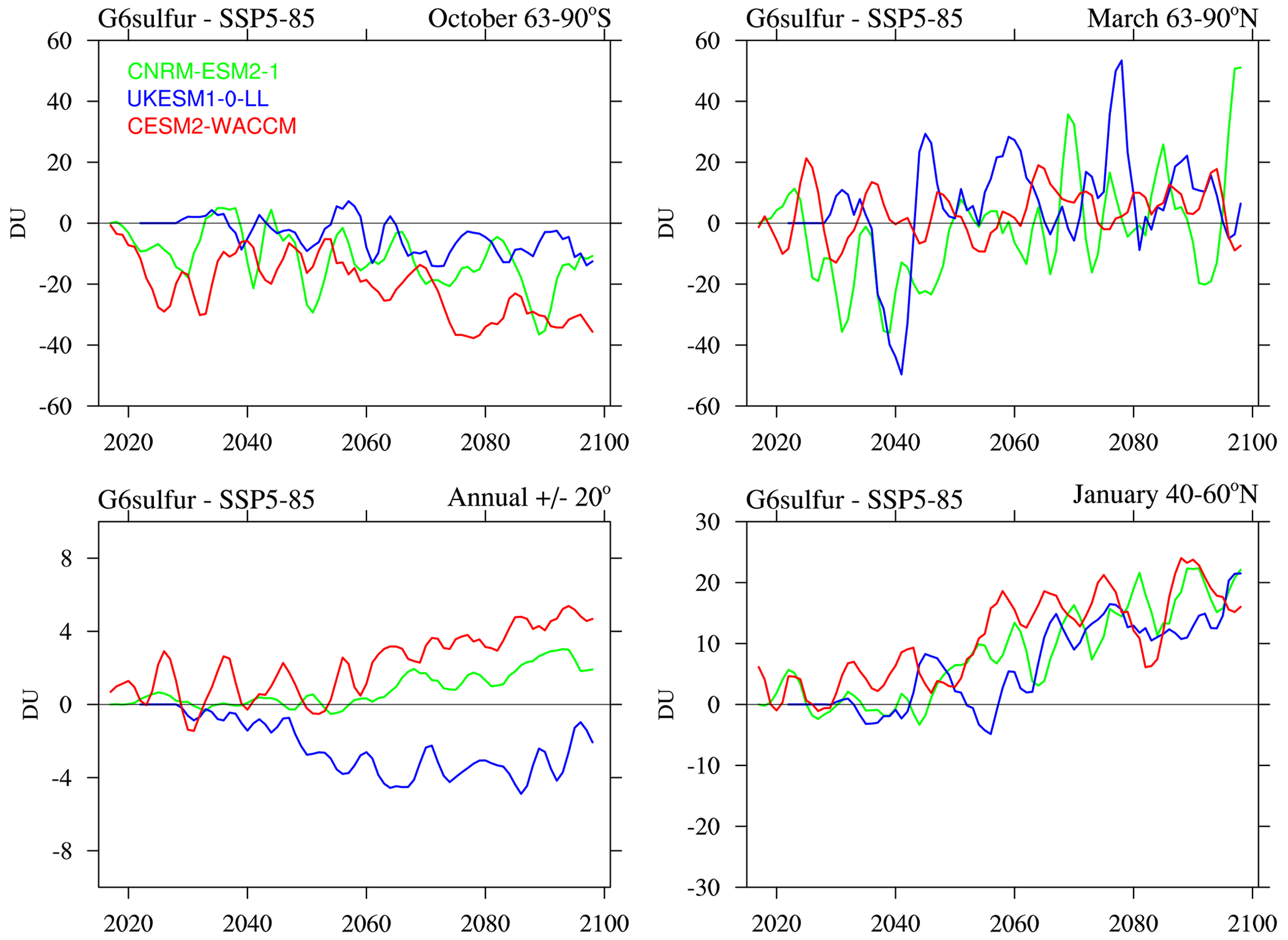
Figure 9 Differences between G6sulfur and SSP5-8.5 for the ensemble mean of total column ozone between 2020 and 2100 for the three different models (colored lines) and for four different seasons and regions (different panels).​​​​​​​

TCO in the NH polar region is strongly controlled by the dynamical variability for different years, in addition to chemical changes. Both CNRM-ESM2-1 and UKESM1-0-LL show much larger interannual variably in TCO compared to WACCM, which is more in line with what has been observed (Keeble et al., 2021). WACCM6 does not show any significant changes in TCO, while CNRM-ESM2-1 shows a reduction in TCO in the first 40 years. Despite no changes in SAD until 2040, this reduction is consistent with the strengthening of the polar vortex in G6sulfur compared to SSP5-8.5. UKESM1-0-LL reproduces an initial reduction in TCO of up to 30 DU by the onset of SAD in 2030. Based on the multi-model mean (Fig. 11; right column) differences in G6sulfur compared to SSP5-8.5 only show an initial decrease by the onset of SAI and a small (below 20 DU) increase in ozone towards the end of the century. Compared to SSP2-4.5, TCO shows a substantial increase of up to 40 DU by the end of the century.

Similar to the NH polar region in March, dynamics and transport strongly impact NH mid-latitudes in winter. A weakening of the STJ results in enhanced meridional transport of air masses towards mid- and high latitudes in G6sulfur compared to SSP5-8.5. All models show a consistent increase in TCO up to 20 DU by the end of the century. WACCM6 shows a stronger initial increase, likely because of the earlier start of SAI. Compared to SSP2-4.5, the multi-model mean reaches above 40 DU. The very robust increase in TCO correlates with the amount of sulfur injections.

The impact of G6sulfur on TCO in the tropics shows a mixed signal (Figs. 8, bottom row, and 9). Both CNRM-ESM2-1 and WACCM6 describe an increase in TCO with SAI, while UKESM1-0-LL shows a decrease compared to SSP5-8.5. Ozone concentrations are increasing around the tropopause for all three models. Both CESM2-WACCM6 and UKESM1-0-LL show a decrease in ozone around 20 hPa, which is most pronounced in UKESM1-0-LL. This is likely driven by the increase in w^∗, as discussed above, and could have a larger effect than the increase in ozone in the upper stratosphere, therefore resulting in a net decrease in TCO in UKESM1-0-LL. In addition, CESM2-WACCM6 shows a stronger increase in ozone above 20 hPa, which is aligned with an increase in SAD in that region, as discussed above. The multi-model mean in the tropics shows non-significant changes between G6sulfur and SSP5-8.5 and an increase in TCO around 2 DU compared to SSP2-4.5.

3.4.2 Effects of solar dimming on TCO

Change in ozone in G6solar compared to SSP5-8.5 are impacted by changes in transport (including w^∗) comparable to SSP2-4.5 conditions, while stratospheric temperatures remain mostly unchanged. In addition, as discussed above, the reduced ozone photolysis due to changes in insolation and reductions in humidity due to the cooling of the troposphere can increase upper atmospheric and tropospheric ozone.

Figure 10 Differences between G6solar and SSP5-8.5 for the ensemble mean of total column ozone between 2020 and 2100 for the three different models (colored lines) and for four different seasons and regions (different panels).

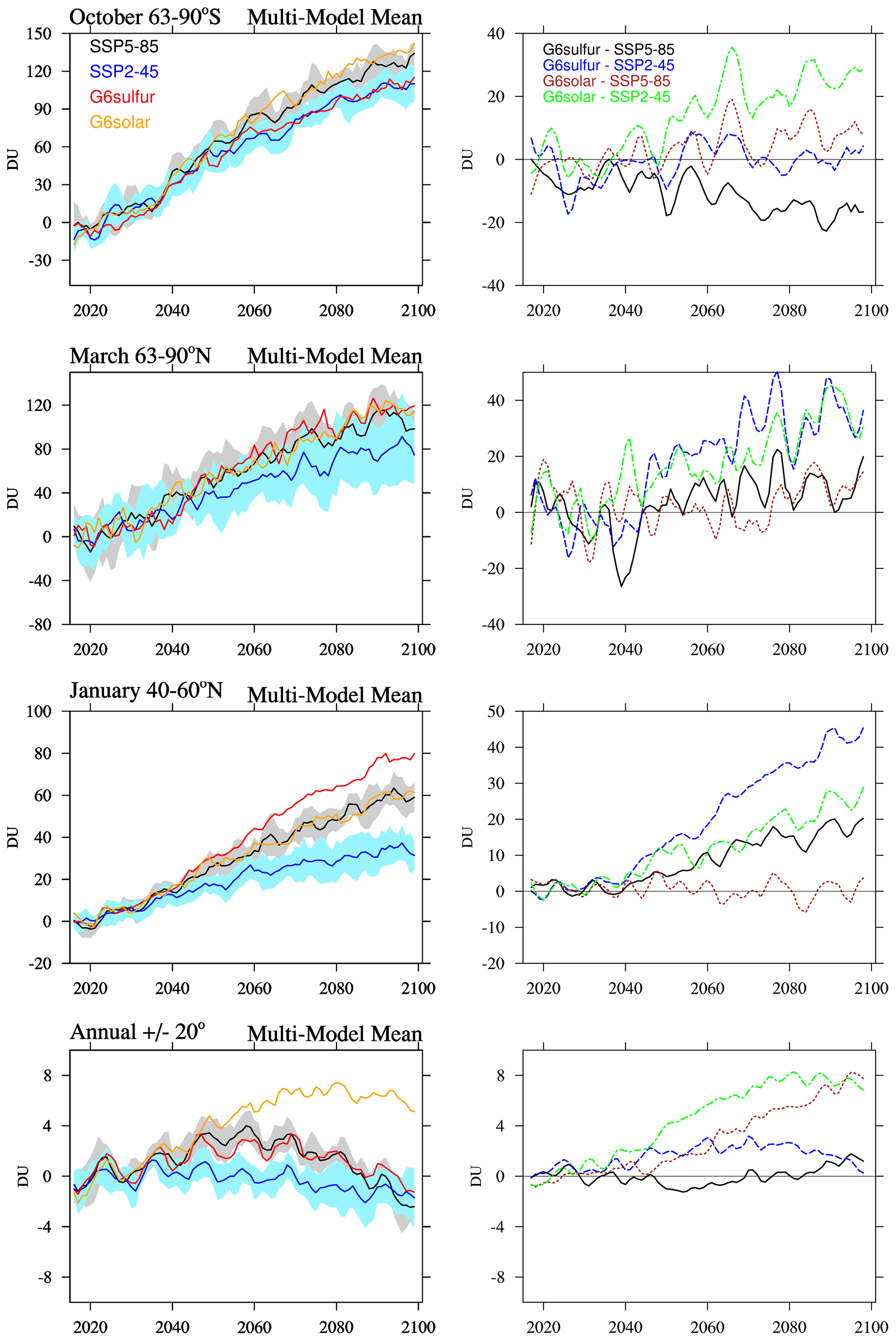
Figure 11 The left column shows the multi-model mean of the total column ozone evolution between 2020 and 2100 normalized to 2020 values for different experiments (different colors) and four different regions and seasons (different rows). The 2σ standard deviation of the ensemble mean is only shown for SSP5-8.5 and SSP2-4.5 scenarios for better readability. The right column shows the differences between G6sulfur and SSP5-8.5 (black lines), G6sulfur and SSP2-4.5 (blue lines), G6solar and SSP5-8.5 (brown lines), and G6solar and SSP2-4.5 (green lines) for the multi-mean of total column ozone between 2020 and 2100 for four different seasons and regions (different rows).

For the SH polar region in October, minor changes in ozone are simulated in all models in the first half of the 21st century (Fig. 10). Only UKESM1-0-LL simulates an increase in TCO of 20 DU, compared to SSP5-8.5, in the last 20 years of the applications. Differences with respect to the other models are likely caused by including the effects of aerosol loading on the photolysis calculation. For the NH polar region in March, CNRM-ESM2-1 shows a decrease in TCO between 2040 and 2080 and an increase after that. UKESM1-0-LL simulates an increase in TCO after 2080, and WACCM6 shows a decrease by the end of the century. Given the large variability in the NH polar region in March, these changes may not be significant. The multi-model mean in high polar latitudes in spring (Fig. 11) shows only a minor increase in TCO below 10 DU by the end of the 21st century compared to SSP5-8.5. However, compared to SSP2-4.5, ozone shows a significant increase up to 30 DU for both hemispheres by the end of the 21st century.

For NH mid-latitudes in January, solar dimming has no significant effect for any of the models. However, for the tropics, solar dimming results in a consistent increase between 4 and 8 DU for the three models, compared to SSP5.8.5, and over 8 DU, compared to SSP2-4.5, in the multi-model mean. This is likely the result of the deceleration of the BDC upwelling.

4 Summary

We used the GeoMIP experiments G6sulfur and G6solar to identify the impacts of SAI and solar dimming on stratospheric ozone. The results from the only three ESMs with comprehensive stratospheric chemistry were used. The G6sulfur and G6solar baseline experiment employ the high climate forcing scenario of SSP5-8.5. SAI and solar dimming are applied to reach surface temperatures of the SSP2-4.5 target experiment. For the analysis of the results, we used limited model output, including zonal mean temperature, zonal winds, aerosol surface area density, and ozone. Some additional quantities, including the vertical component of the TEM circulation, w^∗, were only derived for one model (CESM2-WACCM6).

Both G6solar and G6sulfur applications result in significant changes compared to SSP5-8.5 and SSP2-4.5 with regard to TCO, which differ by region and season. Both model experiments include, per design, reductions in solar radiation reaching the ground (due to the reflection of shortwave radiation by aerosols or to solar dimming) and a decrease in tropospheric temperatures to SSP2-4.5 conditions. Significant differences between the two approaches include the increase in absorbing sulfate aerosols in the stratosphere in G6sulfur, which increases the lower tropical stratospheric temperatures and stratospheric transport, and the increase in aerosol burden and, therefore, SAD.

For G6sulfur, the temperature increase in the lower tropical stratosphere ranges between 5 to 13 K by the end of the century, for the suite of GeoMIP models that performed this experiment, and between 5 to 7 K, for those models that include interactive stratospheric chemistry. The heating of the lower tropical stratosphere by the sulfate aerosol causes a weakening of the subtropical jet, a strengthening of the polar vortex, a reduction in tropical upwelling below the injection location of sulfur, and an increase in the tropical upwelling above the injection locations with respect to SSP5-8.5, as already observed in previous simulations (Pitari et al., 2014; Richter et al., 2017; Visioni et al., 2020; Niemeier et al., 2020). For G6solar, stratospheric temperatures stay close to the conditions in the baseline simulation of SSP5-8.5, while tropospheric temperatures, stratospheric winds, and tropical upwelling are more similar to SSP2-4.5 conditions. In addition to these changes, increasing SADs in G6sulfur compared to G6solar increases chemical production and loss rates due to increasing heterogeneous reactions. An increase in SAD in the high polar latitudes in winter and spring reduces ozone, while increases in the tropics and mid-latitudes and mid- and upper stratosphere increase ozone.

The combination of changes described above impacts TCO in G6sulfur and G6solar in addition to changes from increasing GHGs in SSP5-8.5 and SSP2-4.5. Ozone reduction in G6sulfur under SAI conditions for all three models by the end of the 21st century has been identified only for October in the southern polar latitudes. An initial significant decrease in polar ozone is only simulated in CESM2-WACCM6 because of a strong initial increase in SAD in the polar region between 2020 and 2030. Since the other models required a later start of sulfur injections and may have potential shortcomings in processing ozone loss based on heterogeneous reactions, they initially produced a smaller increase in SAD in high latitudes. The decrease in TCO counteracts the super recovery of TCO in SSP5-8.5 without SAI towards SSP2-4.5 conditions. In northern high latitudes in March, only UKESM1-0-LL shows a strong decrease in TCO at the onset of SAI. The lack of some ozone loss in CESM2-WACCM6 during the onset of SAI may result from NH polar temperatures that are too warm in this model. In the multi-model mean, TCO shows a small increase of up to 10 DU by the end of the 21st century for this region and season. All models consistently show an increase in TCO in the NH winter mid-altitudes as the result of meridional transport of more ozone in the lower tropical tropopause compared to the baseline scenario. On the other hand, the changes in TCO in the tropics are mixed in sign and magnitude among the models, likely because of differences in changes in tropical upwelling, aerosol distribution, and treatment of ozone photolysis.

The impact of solar dimming compared to SAI on ozone is very different in some regions. For October in the SH polar latitudes, one model shows an increase in TCO with increasing solar dimming, while the other two models do not show a significant change. The response in the NH high latitudes in spring is also mixed and does not point to significant changes compared to SSP5-8.5 conditions. Similarly, TCO shows no significant changes at high and mid-latitudes. However, in contrast to G6sulfur, all models show a significant increase in TCO in the tropics with increased solar dimming.

5 Conclusions

Recent literature often states that SAI would lead to ozone loss (e.g., Keith and Irvine, 2016). Here we analyze three independent ESMs and confirm that ozone loss in the high southern latitudes would still be a concern if SAI were to be applied. However, considering this specific scenario and the multi-model mean, reductions in TCO are rather small and only reach 20 DU, compared to SSP5-8.5, and only show initial changes in the first 2 decades, compared to SSP2-4.5. The reason is that two out of three models show no significant ozone loss. Differences in TCO are caused by how much sulfur injection is required to counteract the surface temperature increase between SSP2-4.5 and SSP5-8.5 and how the models represent both relevant physical and chemical processes. Simplified descriptions of stratospheric aerosols and microphysical schemes may not reflect the increase in SAD by the onset of SAI. In summary, all three models with interactive chemistry show shortcomings in representing different processes properly. For instance, CNRM-ESM2-1 uses a prescribed aerosol distribution that does not reflect changes in the aerosols size with emission amount, the UKESM1-0-LL version used here includes limited representation of heterogeneous halogen reactions on sulfate aerosols and simplified ODS to reflect changes in future ozone, CESM2-WACCM does not reproduce Arctic ozone loss very well, and, finally, both CNRM-ESM2-1 and CESM2-WACCM do not include changes in aerosol loading in their photolysis scheme. Improvements in the models are needed and may change the results significantly.

Models agree that the increase in sulfur injections results in a robust increase in TCO in NH winter mid- and high latitudes up to 20 DU, compared to SSP5-8.5, and up to 40 DU, compared to the target scenario SSP2-4.5. This increase in TCO is linearly related to the increase in sulfur injection and is driven by the warming of the tropical lower stratosphere. It would also compound with the pronounced increase in TCO compared to present-day levels that may reach up to 30 DU on an annual average between 30–60^∘ N and 50 DU between 60–90^∘ N, and that is expected because of the super recovery due to climate change (Dhomse et al., 2018; Keeble et al., 2021). This large increase in TCO may have potentially large effects on society and ecosystems and would have to be investigated in detail (Zarnetske et al., 2021). Changes in the tropics using SAI are small and less conclusive, based on the three models.

On the other hand, it has been stated that a less radiatively absorbing material like calcium carbonate would result in a smaller impact on global ozone and may prevent ozone deletion and other related changes (IPCC, 2021). However, this may not be true if one considers solar dimming as an analog to less absorbing or non-absorbing materials. This study shows that solar dimming would not effectively revert TCO to that of the target experiment of SSP2-4.5. In contrast to G6sulfur, solar dimming and, potentially, a less absorbing aerosol would not revert the super recovery of TCO in SSP5-8.5 to SSP2-4.5 conditions in the long run and, therefore, result in significantly larger TCO values around 30 DU, compared to SSP2-4.5, in mid- and high latitudes.

Solar dimming would further significantly increase TCO in the tropics by 4 DU, compared to SSP5-8.5, and by up to 8 DU, compared to SSP2-45. However, this change may counteract the reductions in TCO around 5 DU for SSP5-8.5 and SSP2-4.5 by the end of the 21st century due to climate change. Furthermore, the impact of G6sulfur on TCO is, in part, driven by changes in photolysis rates. Only one model includes the effects of aerosols on photolysis. This particular model shows, in general, more ozone increase within G6sulfur than the other models. This indicates that improvements in the photolysis scheme in models are needed in order to improve the simulation of impacts of SAI and solar dimming approaches on ozone.

Finally, the climate intervention scenarios discussed would require a continued increase in sulfur injections well beyond the 21st century in order to keep surface temperatures to SSP2-4.5 conditions and not result in a phasing-out of SAI. In addition, SSP2-4.5 surface temperature conditions do not describe a feasible target to reach the required surface temperature of 1.5 ^∘C above preindustrial conditions in order to prevent significant impacts and potentially reach tipping points. However, the main finding of the effects of SAI and solar dimming on stratosphere ozone is likely applicable to different lower-forcing experiments.

Appendix A: Supporting figures

This section includes supporting material in the form of additional Figs. A1 to A4, as referred to in the main text.

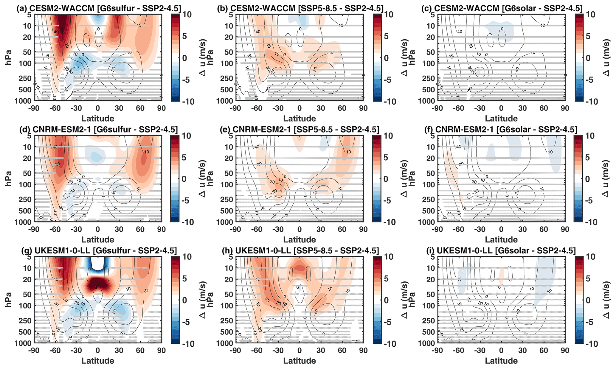
Figure A1 Zonal mean zonal wind changes (m s⁻¹; 2080–2089) between G6sulfur and SSP2-4.5 (a, d, g), SSP5-8.5 and SSP2-4.5 (b, e, h), and G6solar and SSP2-4.5 (c, f, i) for the three GeoMIP models with interactive chemistry that participated in the G6 experiment. Contour lines show the baseline SSP2-4.5 winds. Gray horizontal lines indicate changes that are not statistically significant over the temporal period considered when using a double-sided t test at 95 % confidence levels.

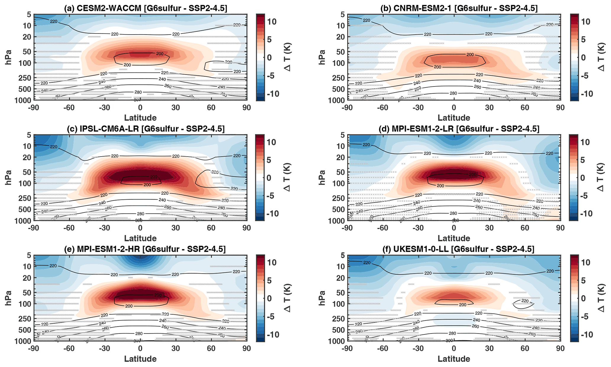
Figure A2 Zonal mean temperature changes (2080–2099) between G6sulfur and SSP2-4.5 for all GeoMIP models participating in the G6 experiment. Contour lines show the baseline SSP2-4.5 temperature. Gray horizontal lines indicate changes that are not statistically significant over the time period considered when using a double-sided t test at 95 % confidence levels.

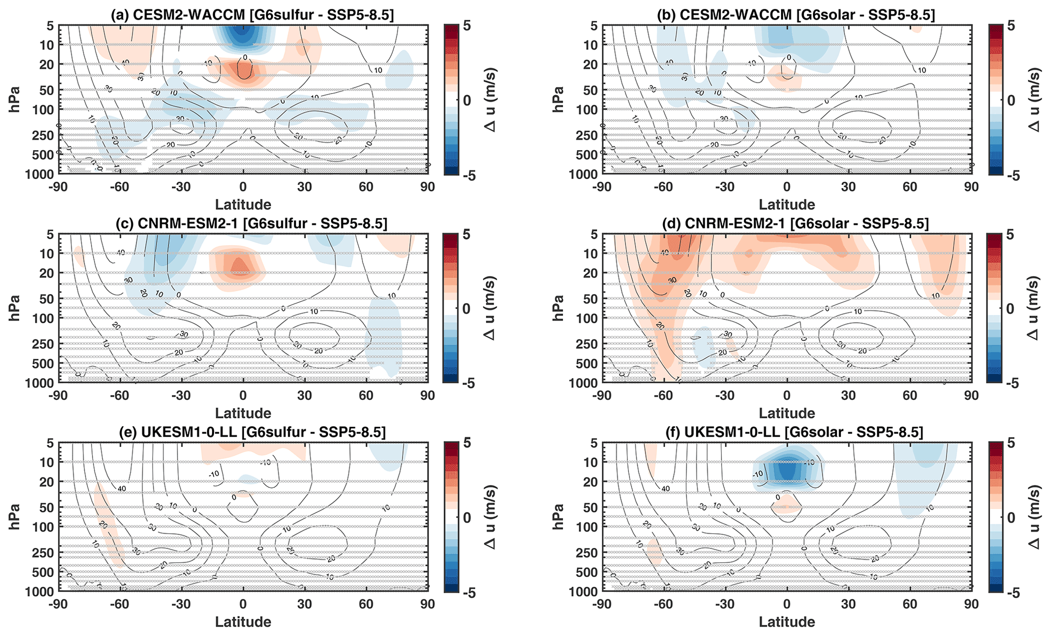
Figure A3 Zonal mean U winds changes (m s⁻¹; 2030–2039) between G6sulfur and SSP5-8.5 (a, c, e) and G6solar and SSP5-8.5 (b, d, f) for the three GeoMIP models with interactive chemistry that participated in the G6 experiment. Contour lines show the baseline SSP5-8.5 winds. Gray horizontal lines indicate changes that are not statistically significant over the time period considered when using a double-sided t test at 95 % confidence levels

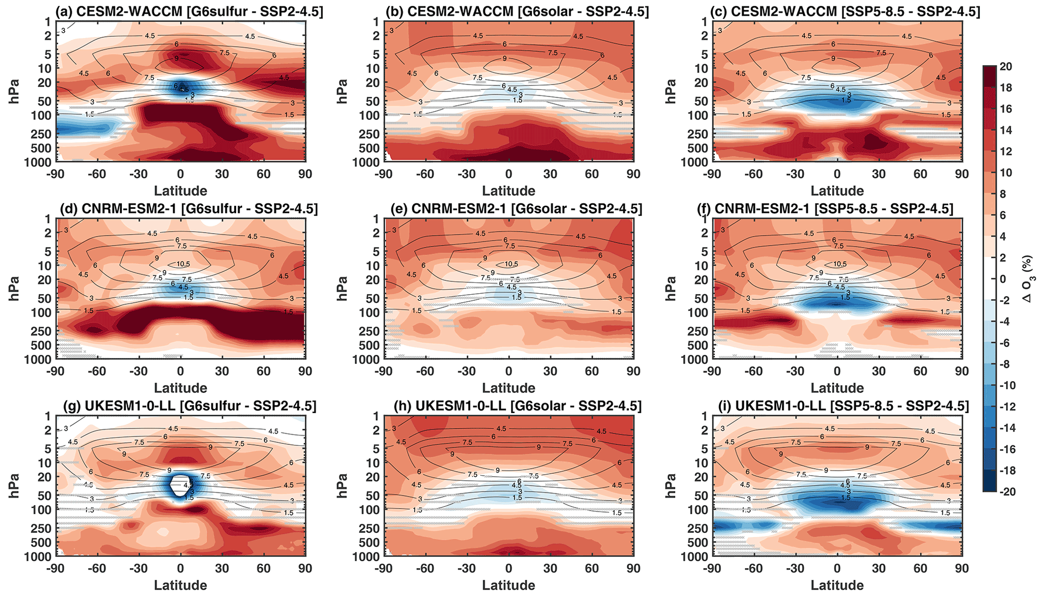
Figure A4 Ozone concentration changes (%) between G6sulfur and SSP2-4.5 (a, d, g), G6solar and SSP2.-45 (b, e, h), and SSP5-8.5 and SSP2-4.5 (c, f, i) in the 2080–2099 period. Contour lines show the SSP2-4.5 ozone concentration over the same period. Gray horizontal lines indicate changes that are not statistically significant over the temporal period considered when using a double-sided t test at 95 % confidence levels.