the Creative Commons Attribution 4.0 License.
the Creative Commons Attribution 4.0 License.
 | 02 Nov 2022
Effects of Arctic ozone on the stratospheric spring onset and its surface impact
Marina Friedel
Gabriel Chiodo
Andrea Stenke
Daniela I. V. Domeisen
Thomas Peter
Ozone in the Arctic stratosphere is subject to large interannual variability, driven by both chemical ozone depletion and dynamical variability. Anomalies in Arctic stratospheric ozone become particularly important in spring, when returning sunlight allows them to alter stratospheric temperatures via shortwave heating, thus modifying atmospheric dynamics. At the same time, the stratospheric circulation undergoes a transition in spring with the final stratospheric warming (FSW), which marks the end of winter. A causal link between stratospheric ozone anomalies and FSWs is plausible and might increase the predictability of stratospheric and tropospheric responses on sub-seasonal to seasonal timescales. However, it remains to be fully understood how ozone influences the timing and evolution of the springtime vortex breakdown. Here, we contrast results from chemistry climate models with and without interactive ozone chemistry to quantify the impact of ozone anomalies on the timing of the FSW and its effects on surface climate. We find that ozone feedbacks increase the variability in the timing of the FSW, especially in the lower stratosphere. In ozone-deficient springs, a persistent strong polar vortex and a delayed FSW in the lower stratosphere are partly due to the lack of heating by ozone in that region. High-ozone anomalies, on the other hand, result in additional shortwave heating in the lower stratosphere, where the FSW therefore occurs earlier. We further show that FSWs in high-ozone springs are predominantly followed by a negative phase of the Arctic Oscillation (AO) with positive sea level pressure anomalies over the Arctic and cold anomalies over Eurasia and Europe. These conditions are to a significant extent (at least 50 %) driven by ozone. In contrast, FSWs in low-ozone springs are not associated with a discernible surface climate response. These results highlight the importance of ozone–circulation coupling in the climate system and the potential value of interactive ozone chemistry for sub-seasonal to seasonal predictability.
- Article
(10367 KB) - Full-text XML
- BibTeX
- EndNote


In spring, as sunlight returns to the polar regions, zonal winds in the stratosphere change direction from winter westerlies, known as the polar vortex, to summer easterlies. This transition from winter to summer in the stratosphere, with major disruptions of the stratospheric zonal flow, is called the final stratospheric warming (FSW) (Black et al., 2006). FSWs are primarily driven by an increase in shortwave radiation in the polar regions in spring in combination with planetary wave forcing (Waugh et al., 1999; Black et al., 2006). While a FSW occurs every year in both hemispheres, its timing is subject to large interannual variability. In the Arctic, FSWs have been observed from as early as mid-March to as late as the end of May (Hu et al., 2014), depending on variations in the upward propagation of tropospheric planetary waves, as well as the stratospheric background flow and temperature (Waugh et al., 1999; Black et al., 2006; Salby and Callaghan, 2007; Hu et al., 2014; Thiéblemont et al., 2019). The timing of the FSW has important consequences for both stratospheric and tropospheric climate and for subseasonal to seasonal predictability (e.g., Ayarzagüena and Serrano, 2009; Thiéblemont et al., 2019; Butler et al., 2019).
As previous studies have shown (Rieder et al., 2019; Haase and Matthes, 2019; Friedel et al., 2022), springtime stratospheric temperature and circulation, which influence the timing of the FSW, are also closely tied to anomalies in stratospheric ozone. While some springs are marked by a warm polar vortex with high ozone concentrations, such as 2021 (Lu et al., 2021; Bahramvash Shams et al., 2022), other years show an extremely cold polar vortex with drastic springtime ozone depletion, e.g., in 2020 (Lawrence et al., 2020; Rao and Garfinkel, 2021b). Stratospheric ozone thereby does not only passively respond to changes in the circulation. Rather, ozone anomalies are thought to actively feed back on stratospheric dynamics via radiative heating (Haase and Matthes, 2019; Oehrlein et al., 2020; Friedel et al., 2022), though uncertainties remain with respect to the magnitude of the ozone effects. Connections between springtime Arctic ozone, planetary wave activity, and the timing of the FSW in the lower stratosphere have previously been reported, with enhanced transport and mixing of ozone-rich air into the Arctic and an earlier vortex breakup in springs when planetary wave activity is strong (Salby and Callaghan, 2007). This link, however, only describes the response of ozone to wave driving, while the role of the resulting ozone anomalies in modulating the dynamics and altering the timing and evolution of the FSW still remains unclear. A clear mechanistic understanding and quantification of the impacts of ozone on the FSW is lacking.
By causing major changes in stratospheric dynamics, FSWs leave their fingerprint on the tropospheric circulation through downward coupling. At the Earth's surface, the FSW tends to shift the North Atlantic Oscillation (NAO) towards its negative phase (Black et al., 2006; Thiéblemont et al., 2019), but surface responses strongly depend on the timing of the FSWs. While early FSWs (Black and McDaniel, 2007b) are usually followed by a negative phase of the Arctic Oscillation (AO) with cold and wet anomalies over central and southern Europe and Eurasia (and thus behave similarly to mid-winter sudden stratospheric warmings (SSWs); Baldwin et al., 2021), late FSWs do not have any robust effects on surface climate (Li et al., 2012). Rather, late FSWs tend to be preceded by a positive phase of the Arctic Oscillation, which shifts to neutral after the FSW date (Black et al., 2006; Ayarzagüena and Serrano, 2009; Thiéblemont et al., 2019). Even though early FSWs usually have a greater surface impact than late FSWs, they are less predictable due to their sudden nature (Butler et al., 2019). If ozone was identified as a modulator of the timing of FSWs, a potential shift in the breakup date of the polar stratospheric vortex by ozone could thus have a large impact on both the FSW predictability and their signature on surface climate.
In other contexts, it has already been established that ozone contributes to stratosphere–troposphere coupling during extreme events. For example, ozone anomalies have previously been shown to enhance downward coupling during SSWs (Haase and Matthes, 2019; Oehrlein et al., 2020). Most notably, Arctic ozone minima have been identified as a crucial driver of the surface circulation in springtime (Friedel et al., 2022). Conversely, a similar connection between ozone and the downward impact of FSWs has not yet been demonstrated. Since many state-of-the-art forecast models still prescribe a diagnostic ozone forcing, they neglect such possible influences of ozone. A better mechanistic and quantitative understanding of the connection between springtime ozone, FSW date, and subsequent surface patterns might lead the way to improved sub-seasonal to seasonal predictions for both the stratosphere and troposphere (Cionni et al., 2011; Eyring et al., 2013; Hersbach et al., 2020; Monge-Sanz et al., 2022). Recent modeling studies on the Southern Hemisphere already show promising results, with an improvement of forecast skill on seasonal timescales arising from stratospheric ozone (Hendon et al., 2020; Oh et al., 2022).
While observations provide information about the statistical correlation of stratospheric ozone and the FSWs, they cannot be used to directly assess the causality of this connection. Further, the observational record is rather short (41 years), and internal variability might be too large to establish a robust connection between ozone and the FSW in observations. Here, we shed new light on the ozone–FSW connection by performing targeted modeling experiments to isolate the impact of Arctic ozone from dynamical variability. Specifically, we address the following questions. (1) How large is the impact of ozone on the timing of the FSW? (2) Is there a significant influence of ozone on the surface response to FSWs? (3) What are the mechanisms whereby ozone modulates the downward coupling during FSWs?
This paper is structured as follows. Section 2 gives an overview over the data and model experiments used in this study as well as analysis methods. Section 3 describes the effects of ozone on the timing of FSWs. Next, we explore the ozone influence on the downward impact of FSWs, highlighting the physical mechanism at work. In Sect. 4 our results are summarized and discussed.
2.1 Input data and design of model experiments
Here we use chemistry–climate models (CCMs) to isolate the effects of ozone anomalies on the FSW and compare our results with observations. To do this, we use two fully independent CCMs, WACCM version 4 and SOCOL-MPIOM, to gain insights into possible model dependencies of the ozone-dynamics coupling.
WACCM, the Whole Atmosphere Community Climate Model, is the atmospheric component of the NCAR Community Earth System Model version 1 (CESM1.2.2). WACCM has a high model top ( hPa) with 66 vertical levels (Marsh et al., 2013) and is coupled to interactive ocean and sea ice components (Danabasoglu et al., 2012; Holland et al., 2012). WACCM has a horizontal resolution of 1.9∘ in latitude and 2.5∘ in longitude (Marsh et al., 2013) and can be run in both an interactive and specified chemistry mode (Smith et al., 2014). When coupled to the interactive chemistry scheme, WACCM calculates ozone concentrations over a set of chemical equations including a total of 59 species (Marsh et al., 2013). When run in specified chemistry mode, ozone concentrations and other radiative species are prescribed in the form of climatologies (Smith et al., 2014). Having been documented to capture stratospheric trends and variability reasonably well, WACCM has been used in many recent studies on interannual stratospheric variability (e.g., Haase and Matthes, 2019; Rieder et al., 2019; Oehrlein et al., 2020).
SOCOL, SOlar Climate Ozone Links, version 3 is a CCM based on the general circulation model MA-ECHAM5, which is interactively coupled to the chemistry transport model MEZON (Model for Evaluation of oZONe trends; Egorova et al., 2003) and to the ocean–sea ice model MPIOM (Stenke et al., 2013; Muthers et al., 2014). SOCOL-MPIOM has a model top at 0.01 hPa and 39 vertical levels and is used here at a horizontal resolution of T31 (3.75∘ × 3.75∘) (Stenke et al., 2013). SOCOL-MPIOM can be run in an interactive chemistry mode, including a set of 140 gas-phase, 46 photolysis, and 16 heterogeneous reactions involving 41 species. Like WACCM, SOCOL-MPIOM can also be run in a specified chemistry configuration by decoupling the chemistry module and general circulation model, in which case ozone concentrations are prescribed as climatologies (Muthers et al., 2014). Like WACCM, SOCOL-MPIOM captures stratospheric variability reasonably well (Muthers et al., 2014).
To isolate ozone–circulation coupling, we simulate two different setups with both CCMs, WACCM and SOCOL-MPIOM: one with fully interactive ozone chemistry (INT-3D) and one with prescribed, climatological ozone (CLIM-3D) (Friedel et al., 2022). The latter is forced by a daily, three-dimensional ozone climatology derived from experiments with fully interactive chemistry from each respective model. In contrast to other studies using similar approaches (e.g., Haase and Matthes, 2019), the experiments with prescribed ozone (CLIM-3D) still employ the chemistry scheme; i.e., the ozone field is still calculated but not seen by the radiation. Thus, the calculated ozone in these runs acts as a passive tracer and serves as a dynamical proxy without exerting dynamical feedbacks. The calculated ozone field of both CLIM-3D and INT-3D simulations is later used for analysis purposes. With this setup, we find differences between INT-3D and CLIM-3D simulations for specific situations (e.g., FSWs) that can solely be attributed to the two-way coupling between ozone and circulation. A schematic illustration of the model setup is shown in Fig. 1. With both CCMs, we run a total of 200 model years with a fully coupled ocean for both the interactive and noninteractive chemistry configuration. This extension (200 years) delivers reasonable statistics in the context of FSWs (Thiéblemont et al., 2019). All model simulations are forced by present-day boundary conditions of the year 2000 for greenhouse gases (GHGs) and ozone-depleting substances (ODSs), thus omitting trends due to changes in GHG concentrations or ozone (Friedel et al., 2022), in contrast to studies using transient simulations (Haase and Matthes, 2019). Boundary conditions were set following the CMIP5 forcing datasets (Meinshausen et al., 2011) with fixed, seasonally varying GHG and ODSs, resulting in large springtime ozone variability due to high ODS loading around the early 2000s.
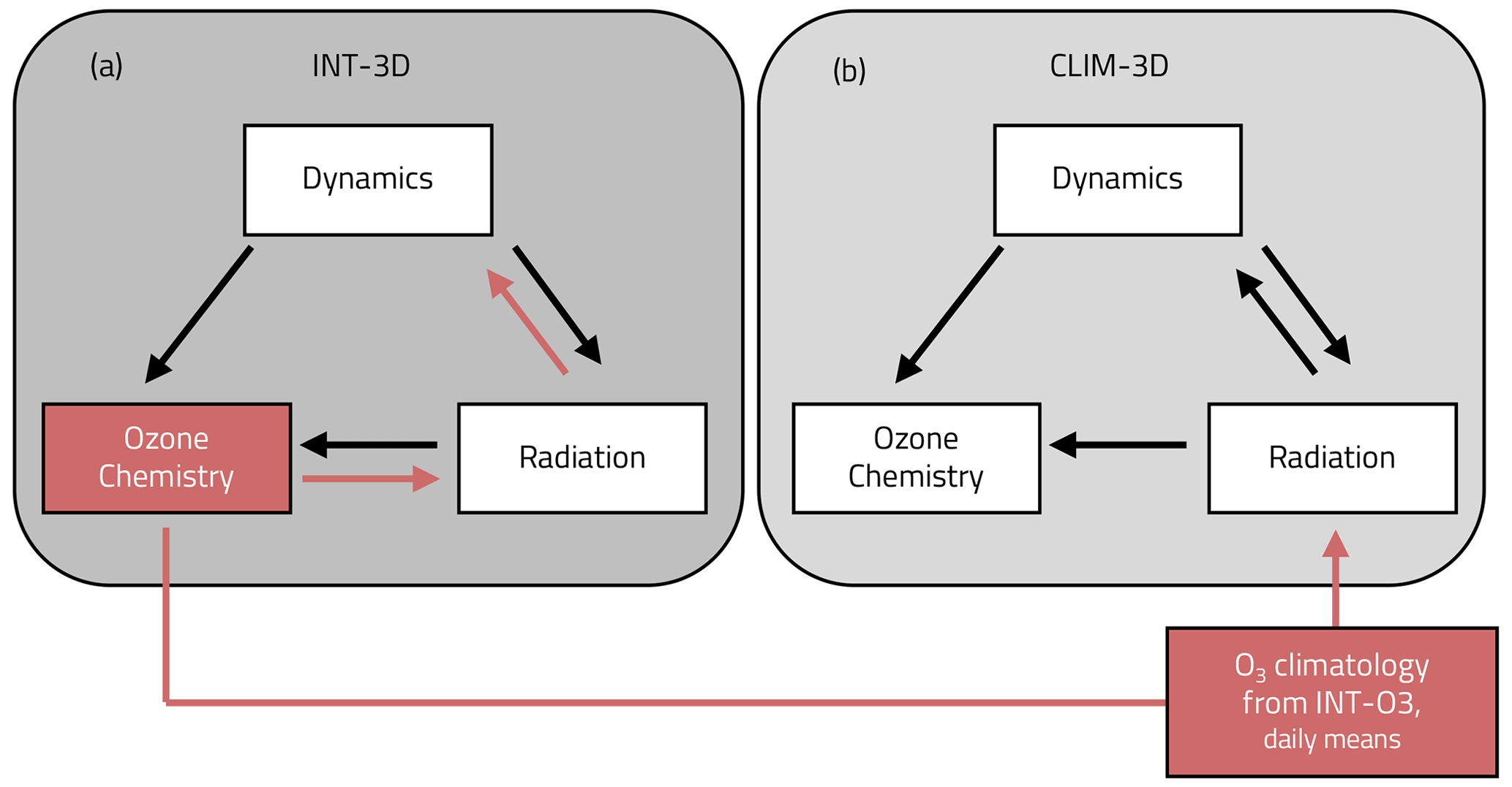
Figure 1Simulation setup. INT-3D (a) uses a fully interactive chemistry module determining the ozone concentrations as they occur during the run, allowing differences to evolve, in particular from one polar winter to the next, directly feeding back into the model's radiation schemes and thus the model's dynamics. In contrast, CLIM-3D (b) is forced by prescribed, daily 3D climatological ozone fields, identical from one year to the next, which have been derived by averaging model runs with fully interactive chemistry (from each respective model, WACCM or SOCOL-MPIOM). The experiments with prescribed ozone (CLIM-3D) still employ the chemistry scheme; i.e., the ozone field is still calculated and affects other radiatively active gases such as methane but does not feed back into the model's radiative scheme (figure adapted from Friedel et al., 2022).
We compare our modeling results with the reanalysis product MERRA2, the Modern-Era Retrospective Analysis for Research and Applications version 2, from 1980 to 2020 (Gelaro et al., 2017). MERRA2 has a horizontal resolution of 0.5∘ × 0.625∘ and 72 hybrid-eta levels from the surface up to 0.01 hPa, and we use 6-hourly instantaneous data output. MERRA2 has been shown to realistically reproduce ozone variability with stratospheric ozone agreeing reasonably well with satellite ozonesonde data (Wargan et al., 2017; Davis et al., 2017; Bahramvash Shams et al., 2022).
2.2 Analysis methods
A variety of different metrics have been used in the past to define the onset of FSWs. While most FSW definitions are based on stratospheric zonal wind at a given altitude falling below a certain threshold (Black and McDaniel, 2007a; Ayarzagüena and Serrano, 2009; Hu et al., 2014; Kelleher et al., 2020; Rao and Garfinkel, 2021a), some studies consider two (Black et al., 2006; Butler and Domeisen, 2021) or multiple different pressure levels (Hardiman et al., 2011; Jinggao et al., 2013; Thiéblemont et al., 2019), and the thresholds used vary. Here, we follow the definition used by Butler and Domeisen (2021), who define the FSW date based on zonal mean zonal wind at 10 and 50 hPa falling below thresholds of 0 and 5 m s−1, respectively. Additionally, we extend this metric to all available pressure levels between 50 and 1 hPa to examine the impacts of ozone on the timing of the FSW throughout the stratosphere. To this end, we define the altitude-dependent FSW onset date on a given pressure level as the first day of the year when zonal mean zonal wind at 60∘ N has fallen below a threshold of 0 m s−1 for altitudes equal to or above 10 hPa and 7 m s−1 for pressure levels lower than 10 hPa and does not return above this threshold for more than 10 consecutive days until the following fall. Adjustment of the wind threshold to 7 m s−1 for lower stratospheric altitudes was necessary to allow the CCMs to generate a FSW every single year, correcting their vortex biases (Stenke et al., 2013; Butchart et al., 2011; Bergner et al., 2022). The polar vortex bias results in a delay of the FSW compared to reanalysis (in our models by 2–3 weeks). This late FSW bias is typical for climate models and has been reported for nearly all CMIP5 and CMIP6 models (Butchart et al., 2011; Rao and Garfinkel, 2021a). The results presented below are insensitive to variations in the wind threshold chosen for determining the FSW onset date, as sensitivity tests with WACCM for thresholds between 3 and 10 m s−1 show. To get insights into the vertical structure of the FSWs, we compare the FSW date at 1 and 10 hPa to distinguish between FSWs happening first at 1 hPa (“1 hPa-first”) and those happening first at 10 hPa (“10 hPa-first”) (Hardiman et al., 2011). If the difference between the FSW date at 1 and 10 hPa is smaller than 5 d, the FSW is considered “neutral” (Hardiman et al., 2011; Thiéblemont et al., 2019).
We investigate the impact of ozone anomalies on the FSW in springs where stratospheric ozone concentrations are unusually high or low. High- and low-ozone springs are defined based on daily zonal mean ozone mixing ratios averaged over the polar cap (60–90∘ N). Unless otherwise specified, the data are first weighted by the cosine of latitude for spatial averaging. To smooth the daily variability and therefore reduce the influence of outliers, a 5 d running mean is computed from the daily ozone data. From the 5 d running mean, we calculate partial column ozone between 30 and 70 hPa, since ozone variability maximizes at different altitudes within this range across datasets (Friedel et al., 2022). For each of the 200 model years we then pick the days with minimum or maximum ozone values over the period from 1 March until the onset of the FSW. The time period was chosen as such that it contains the largest ozone variability, which usually maximizes within March and the FSW (Friedel et al., 2022). Ozone values selected this way are ranked, and the quartile of springs with the lowest minimum or highest maximum daily 5 d running mean partial ozone column are considered “low-ozone springs” and “high-ozone springs”, respectively. The day for which the ozone minimum or maximum occurs is termed “central ozone date”. The simulated (but radiatively noninteractive) ozone field in CLIM-3D experiments allows us to use the same methodology to find ozone minima and maxima also in this configuration, where low or high ozone is a proxy for a strong or weak spring polar vortex, respectively.
We use the transformed Eulerian mean (TEM) framework to study effects of ozone on stratospheric dynamics and planetary wave breaking (Andrews and McIntyre, 1976). Specifically, we use the divergence of the Eliassen–Palm flux (EPF) as a measure for the forcing exerted by planetary waves on the zonal mean flow. The components of the EPF vector in spherical, log-pressure coordinates () are given by
with the three-dimensional velocity (), the Coriolis parameter f, the Earth's radius a, and the temperature-dependent atmospheric density profile ρ0 (Andrews et al., 1987). Using both components of the EPF, we calculate and scale the EPF divergence according to
In regions with EPF convergence (), wave drag results in a deceleration of the zonal flow due to enhanced wave dissipation. In contrast, in regions with EPF divergence (), zonal wind accelerates as a result of the missing drag.
To quantify the surface response of FSWs, we calculate anomalies by computing a climatology of the variable of interest for each day of the year over all years in the dataset, which is subsequently subtracted from the daily values. For MERRA2, climatologies are calculated over the period 1980 to 2019 only, since spring 2020 was characterized by record-breaking surface anomalies (Lawrence et al., 2020), which might skew the climatology due to the short observational record. Further, we use the Arctic Oscillation (AO) index at the surface (1000 hPa) as an indicator for the surface pattern following FSWs. The AO is a measure for the tropospheric large-scale variability in the Northern Hemisphere (NH) with its positive and negative phases having different implications for regional climate (Baldwin and Dunkerton, 2001). Here, we use empirical orthogonal functions (EOFs) to calculate the AO index based on method 3 in Baldwin and Thompson (2009): first, we calculate the EOF loading pattern from year-round geopotential height anomalies north of 20∘ N after applying latitudinal weights using the square root of the cosine of latitude (Baldwin and Dunkerton, 2001). Following this, we regress daily geopotential height anomalies onto the spatial EOF pattern to find the principal component (PC) time series, which is then weighted to unit variance to obtain the AO index.
Bootstrapping is performed to assess the significance of our results, as done in, e.g., Thiéblemont et al. (2019), Haase and Matthes (2019), Oehrlein et al. (2020), and Friedel et al. (2022). To assess whether surface anomalies are significantly different from zero, a one-sample bootstrapping test is performed, for which anomalies are sampled with replacement around the respective FSW dates in random years within each dataset to create a number of samples equalling those contained in the original composite. We repeat this process 500 times to build a probability density function (PDF) of random composites. The actual composite is considered significantly different from its climatology if it differs by 2 or more standard deviations from the mean of the PDF. This procedure indicates significance at the 4.6 % level. Similarly, a two-sample bootstrapping test is performed to check the significance of differences between two datasets. For this purpose, random composites are created for each dataset according to the procedure described above, and the difference between these composites is taken. Repeating this procedure 500 times, we create a PDF of 500 random samples and consider the difference between two datasets to be significant if it differs by two or more standard deviations from the mean of the PDF.
3.1 The impact of ozone on the timing of the final stratospheric warming
We first evaluate the effects of ozone anomalies on the FSW date over the entire depth of the stratosphere. To this end, we select the 25 % of springs with the highest and lowest ozone concentrations and investigate the deviation of the FSW date from its (long-term) mean in the respective high- and low-ozone springs. Below 10 hPa, the FSW is delayed in low-ozone springs, as clearly seen in the MERRA2 reanalysis in Fig. 2c. In contrast, an early FSW is found in high-ozone springs (Fig. 2c). In the upper stratosphere (above ∼ 10 hPa), the opposite behavior is observed: while years with high ozone show a delay in the FSW date at these levels, years with low ozone instead show a neutral FSW date with a tendency towards an earlier breakup (Fig. 2c).
Model simulations with WACCM and SOCOL-MPIOM reproduce the ozone–FSW connection found in the reanalysis. In both models, the FSW at altitudes below ∼ 10 hPa is delayed in springs with low ozone and occurs earlier than on average in springs with high ozone (Fig. 2a, b), with a tendency towards opposite effects in the upper stratosphere. While this is the first time the statistical relationship between ozone and the timing of the FSW is shown across the stratosphere, these results are not surprising following earlier studies (e.g., Salby and Callaghan, 2007). However, these results do not show whether ozone actively modulates the FSW. To assess the latter, we compare simulations with and without interactive ozone chemistry and find major differences between INT-3D and CLIM-3D experiments (solid and stippled lines in Fig. 2a, b). Simulations with interactive ozone chemistry (INT-3D) show larger shifts towards early and late FSWs in high- and low-ozone springs, respectively, below ∼ 10 hPa than those with prescribed ozone (CLIM-3D). Furthermore, the shift in INT-O3 is generally in better agreement with reanalysis. Since the ability of ozone to affect the dynamical coupling is what differs INT-3D from CLIM-3D, we can attribute differences in the timing of the FSW between those simulations solely to ozone. Ozone anomalies thus shift the vortex breakup in the region below ∼ 10 hPa to earlier and later dates in high- and low-ozone springs, respectively, and thereby increase the variability in the timing of the FSW significantly. Differences in the timing of the FSW between INT-3D and CLIM-3D decrease with altitude (solid and stippled lines in Fig. 2a, b) and fully vanish at around 1 hPa. While in SOCOL-MPIOM differences in the timing of the FSW between INT-3D and CLIM-3D are significant even up to an altitude of 3 hPa, in WACCM those differences are only significant in the lower stratosphere (see circles in Fig. 2). In the following, we thus primarily focus on the FSW at 50 hPa, where ozone has the largest impact.
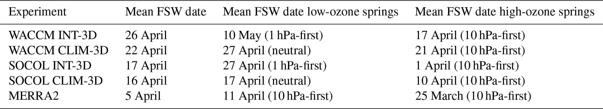
Table 1 shows the mean 50 hPa FSW date as well as the mean FSW dates in low- and high-ozone springs for all model experiments and MERRA2. In the reanalysis, the FSW at 50 hPa happens on average on 5 April, while being delayed by 6 d in low-ozone springs and 11 d early in high-ozone springs. Again, ozone anomalies increase the variability in the breakup dates by pushing the FSW to later and earlier dates in low-ozone and high-ozone springs, respectively, as comparison of breakup dates in INT-3D and CLIM-3D experiments shows (see Table 1). Table 1 gives further information on the mean vertical structure of the FSW in high- and low-ozone springs. In the models, FSWs in low-ozone springs resemble “1 hPa-first” FSWs, whereas FSWs in high-ozone springs tend to occur first at 10 hPa. Most notably, in low-ozone springs, ozone impacts the vertical structure of the FSWs, changing it from “neutral” (as in CLIM-3D) to a “1 hPa-first” pattern (as in INT-3D) in the models.
These results suggest a causal relationship between stratospheric ozone and the timing of the FSW. To examine the role of stratospheric ozone as a precursor to FSWs, we investigate the connection between the FSW date and concomitant ozone concentrations, using all years at our disposal from the model simulations (200 years) and observations (40 years). To this end, we select the maximum value of the 5 d running mean partial ozone column between 20 February (the earliest occurrence of a FSW in our model simulations) and the onset of the FSW in each year of our record, and show its correlation with the FSW date of each year in Fig. 3. In the MERRA2 reanalysis, we find a negative correlation between ozone and the FSW. However, we cannot establish a causal relationship between ozone and the timing of the FSW from the reanalysis and the observational record is too short to establish the robustness of the ozone-FSW link (Thiéblemont et al., 2019). For an improved attribution, we focus on the model simulations. Despite large variability, there is a correlation between the FSW date and preceding ozone anomalies in model simulations using interactive ozone with a Pearson correlation coefficient of approximately −0.30 for both models in the interactive ozone runs (Fig. 3a, b). Linear regression of the FSW date (y axis) against ozone (x axis) reveals a statistically significant negative slope. Thus, the connection between ozone and the timing of the FSW still holds when all years in the record are considered as opposed to only the 25 % strongest ozone anomalies. However, most crucially, the causality of this relationship becomes clear by comparing the INT-3D against CLIM-3D simulations (which do not incorporate interactive ozone). For these experiments, the correlation coefficient decreases considerably (−0.10 and −0.04, as compared to ∼0.30 in the INT-3D runs) and the slope of the linear regression reduces to almost zero (Fig. 3d, e). Additional analysis reveals that differences between INT-3D and CLIM-3D are insensitive to the time frame in which the ozone values are chosen (tested for ±10 d). Thus, both the robustness and the strength of the link between ozone and the FSW date weakens when ozone impacts are neglected. These results confirm the active role of ozone in determining the timing of FSWs, rather than ozone simply being a passive tracer of dynamical variability. Most remarkably, the stronger coupling between ozone and the timing of FSWs is robust across the two models examined here, with the correlation coefficient between ozone and the FSW date increasing by around ∼0.20 when ozone impacts are being considered. The robustness of this ozone–FSW connection over all years in our record and comparison with the reanalysis data is shown in Fig. A3 in Appendix A.

Figure 2The impact of ozone on the FSW date at different altitudes. The mean FSW date in the years with the 25 % highest ozone (red) and the years with the 25 % lowest ozone (blue) at different altitudes compared to the mean FSW date in all years in (a) WACCM, (b) SOCOL-MPIOM, and (c) MERRA2. Datasets cover 200 years for WACCM and SOCOL-MPIOM and 41 years for MERRA2. Solid lines show the mean FSW dates in the INT-3D model evaluation and in MERRA2, and stippled lines show the same information in CLIM-3D. Shaded areas show the standard deviation of the FSW date in INT-3D (a, b) and in MERRA2 (c). Circles mark altitudes where the FSW dates in high- or low-ozone springs between INT-3D and CLIM-3D differ significantly, according to a two-sided Student's t test at the 5 % level.

Figure 3Correlation of the FSW date and preceding springtime ozone. Linear regression of the maximum 5 d running mean partial ozone column between 20 February and the FSW on the deviation of the FSW date from its mean in the respective year in WACCM INT-3D (a), SOCOL-MPIOM INT-3D (b), MERRA2 (c), WACCM CLIM-3D (d), and SOCOL-MPIOM CLIM-3D (e). Colors represent the AO index in the month after the FSW date, solid grey lines show the linear regression. “R” denotes the Pearson correlation coefficient. Vertical stippled grey lines mark the mean ozone value over all years. Mean AO indices are given for years with especially high (right) or low (left) ozone.
Table 1FSW dates at 50 hPa in high- and low-ozone springs. Mean FSW dates in high-ozone and low-ozone years and mean FSW date at 50 hPa over all years in WACCM and SOCOL-MPIOM for both INT-3D and CLIM-3D, as well as for MERRA2.
3.2 The impact of ozone on the surface response of final stratospheric warmings
We now evaluate the surface impacts of FSWs by analyzing the Arctic Oscillation (AO) and show the AO index as color coding in Fig. 3. In the models (Fig. 3a, b, d, e) it can be clearly seen that FSWs preceded by positive ozone anomalies (right side of the scatterplot) are predominantly followed by a negative phase of the AO (red dots). The mean AO index in the month after the FSW is significantly negative in INT-3D simulations following positive ozone anomalies (−0.28 for WACCM and SOCOL, Fig. 3a, b), while the AO index is close to zero and differs across the two models in years with negative ozone anomalies (0.06 for WACCM and −0.13 for SOCOL, Fig. 3d, e). A similar pattern is seen in CLIM-3D (high ozone being connected with early FSWs and a negative AO), but the magnitude is smaller than in INT-3D.
To better quantify the effect of ozone on the FSW surface response, we focus again on high- and low-ozone springs. In Figs. 4 and 5, we show the average sea level pressure (SLP) and surface temperature anomalies for the NH in the 30 d following the 50 hPa FSW in the 25 % highest-ozone (Fig. 4) and lowest-ozone (Fig. 5) springs. In high-ozone springs, both models and reanalysis show positive SLP anomalies over the pole and negative SLP anomalies over the midlatitudes, as expected for a negative AO and seen in Fig. 4a–c. Consistent with a negative AO phase, the SLP anomalies are accompanied by cooling over Eurasia and Europe (Fig. 4f–h). Overall, surface patterns in simulations with interactive ozone (INT-3D) and reanalysis agree reasonably well, although the reanalysis shows a somewhat less zonally symmetric surface response than the models. The smaller zonal symmetry in the reanalysis is due to the smaller number of FSWs in the composite (40 FSWs in the observations vs. 200 FSWs in the models), as can be shown by analyzing a sub-sample of high-ozone springs in model simulations with the same sample size as of the observations (not shown). Our results are consistent with previous literature reporting a shift towards a negative AO after early FSWs, as predominantly found in springs with high ozone (Black et al., 2006; Ayarzagüena and Serrano, 2009). FSWs that tend to be 10 hPa-first have also been associated with a negative AO (Hardiman et al., 2011; Thiéblemont et al., 2019), consistent with the vertical structure and surface response of FSWs in high-ozone springs displayed in Fig. 2. To test whether ozone anomalies affect not only the timing but also the surface response of FSWs, we compare the surface patterns of INT-3D and CLIM-3D simulations. Simulations without interactive ozone (CLIM-3D) show weaker surface anomalies in the 30 d after the FSW in high-ozone springs than INT-3D simulations (Fig. 4d, e, i, j), in line with the smaller AO index in CLIM-3D experiments seen in Fig. 3. Ozone thereby contributes 50 % or more to regional temperature and SLP anomalies in these years and is thus a prominent driver of springtime surface climate in the NH. Again, most importantly this result is robust across the two models used in this study, lending confidence to our findings.
Now that we have established the effects of high ozone concentrations on the surface signature of FSWs, we look at the other extreme, i.e., low-ozone anomalies. In general, we see that in low-ozone springs, FSWs have barely any surface impact (Fig. 4a–e). While WACCM shows a surface patterns which is a reminiscent of a positive AO with pressure anomalies of up to ±4 hPa, SOCOL-MPIOM and the reanalysis do not show any clear AO pattern. Comparison of INT-3D and CLIM-3D simulations in Fig. 4 shows that ozone anomalies do not significantly modulate the surface pattern after FSWs in low-ozone springs in SOCOL-MPIOM, while ozone seems to enhance the surface effects of FSWs in low-ozone springs in WACCM. Hence, the effect of low-ozone anomalies on surface climate following FSWs is not robust across models.
The analysis so far focuses on the 30 d averaging after the onset of the FSW, which masks considerable intra-seasonal variability. To gain additional insights into the role of precursors, we analyze the seasonal evolution of the SLP signal (Figs. 6, 7). For low-ozone cases, the SLP anomaly already emerges in the first half of April and maximizes in mid-April – almost 1 month before the mean FSW date in those years (10 May in WAACM INT-3D). FSWs in low-ozone springs therefore tend to be preceded by SLP anomalies resembling a positive AO. The surface pattern in low-ozone years is thereby not a consequence of the FSW, but results from the preceding ozone minimum, which strengthens the polar stratospheric vortex, resulting in a shift towards a positive AO at the surface (Friedel et al., 2022). Since surface anomalies are more pronounced in simulations including interactive ozone (compare the top and bottom panels in Fig. 7), it can be concluded that the negative ozone anomalies are the cause for the positive AO pattern in low-ozone years. This finding is in line with previous results by Friedel et al. (2022) reporting a shift towards the negative phase of the AO and associated surface climate anomalies driven by strong springtime ozone minima. Here, we show in addition to Friedel et al. (2022) the seasonal evolution of the ozone-induced surface signal and find that the decay of the SLP anomalies occurs simultaneously with the onset of the FSW. Around the time of the FSW (on average on 10 May in WACCM INT-3D), the SLP anomalies start to decay and the AO signal vanishes. The FSW therefore counteracts the surface effects of the ozone minima and offsets their AO response. Thus, the negligible surface anomalies following the FSW in low-ozone springs (as shown in Fig. 5) do not contradict results in Friedel et al. (2022) but are a consequence of the different timings relative to which surface effects are being considered (timing of ozone minima vs. timing of FSW).
Similarly, for high-ozone cases, a shift towards a negative AO pattern can be seen after the onset of the FSW in mid-April (Fig. 6), which is more pronounced in simulations that employ interactive ozone. This shift towards a negative AO following the FSW in both low- and high-ozone springs is consistent with previous findings reporting a decrease of the AO index following FSWs (Thiéblemont et al., 2019). Analysis of the seasonal evolution of the surface AO index also confirms that in our models, FSWs in both low- and high-ozone springs tend to be accompanied by a decrease in the AO index. Moreover, the AO evolution in high- and low-ozone springs, as depicted in Fig. A4 in Appendix A, clearly shows that both the surface signal preceding FSWs in low-ozone springs (blue lines) and following FSWs in high-ozone springs (red lines) is enhanced and longer lived in simulations with fully interactive ozone (compare the top and bottom panels in Fig. A4).
While both SOCOL-MPIOM and WACCM show a similar surface pattern following FSWs in high-ozone springs (Fig. 4), their surface pattern in low-ozone springs differs (Fig. 5). To examine where the model differences in low-ozone springs come from, we analyze possible dependencies of the surface signal on the respective timing of the ozone anomalies and the FSW. The time lag between the central ozone date and the FSW for ozone minima (blue line) differs between models. In WACCM, the FSW happens roughly 1 month after the ozone minimum, when the impacts of the ozone minimum are still present at the surface. The positive AO in WACCM in Fig. 5a is thus a remainder of the downward impact of the preceding ozone minimum. In SOCOL-MPIOM, however, there is a time lag of almost 2 months between the ozone minimum and the FSW. Thus, at the time of the FSW, the surface signal induced by the ozone minima has already completely decayed in this model, leading to slightly different surface patterns after FSWs in low-ozone springs across models, as seen in Fig. 5. The model differences in the timing of those events likely result from differences in the spring planetary wave driving across the model, with a reduced wave driving in WACCM leading to a slower breakup of the polar vortex (see Fig. A5).
In summary, our results show that ozone not only impacts the timing of the FSW but also contributes significantly to the surface response of FSWs. While the shift of the FSW date in high- and low-ozone springs is of equal magnitude (around 10 d in the lower stratosphere), the impact of ozone on the FSW surface response is not equally robust in high- and low-ozone springs. Rather, in low-ozone springs, surface effects and the contribution of ozone anomalies are not robust across models due to differences in the timing of the FSWs. However, ozone strengthens the surface response of the FSWs in high-ozone springs – an effect that is both significant and robust among models.
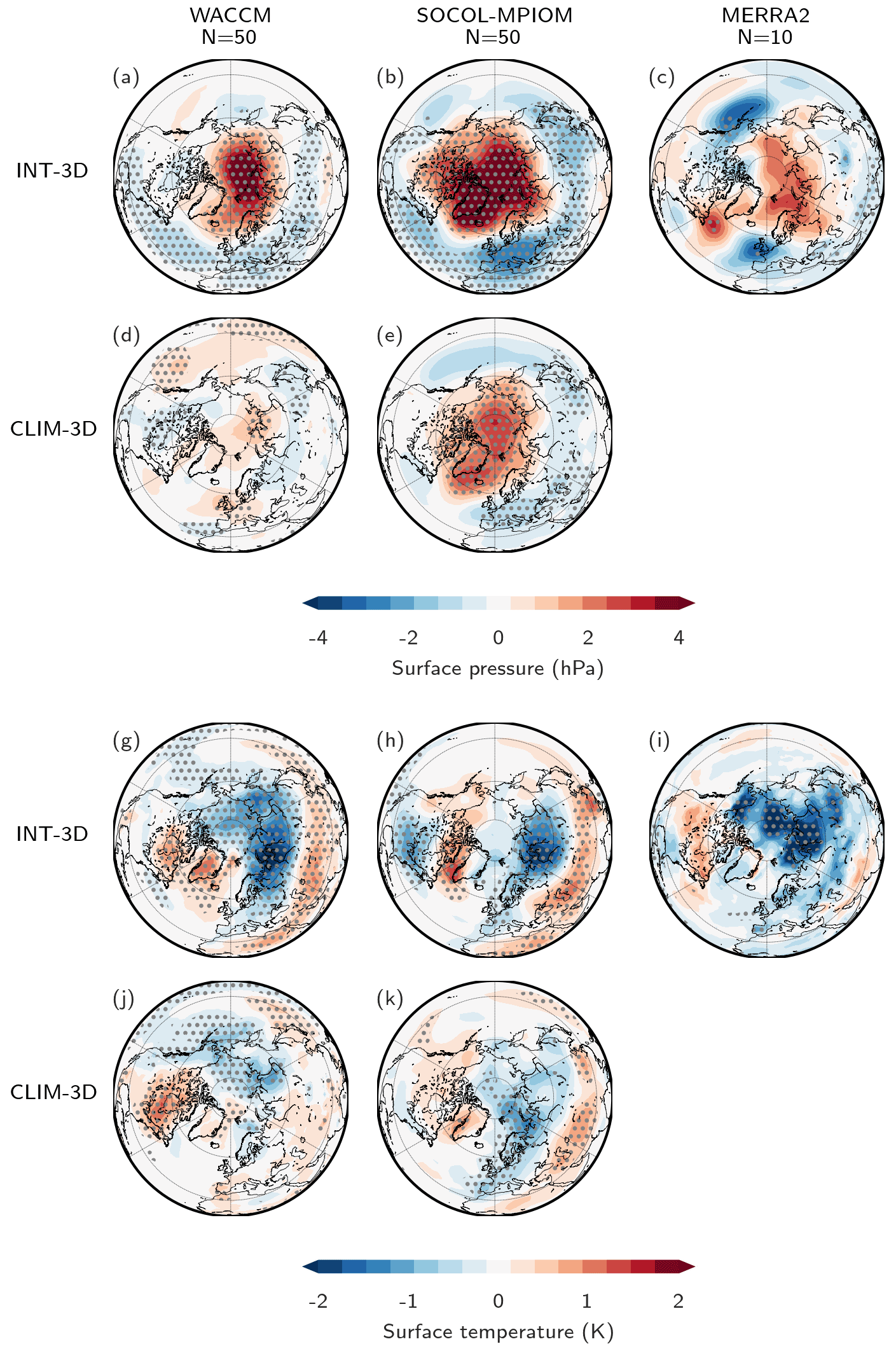
Figure 4The surface impact of FSWs in high-ozone springs and the impact of ozone. SLP (a–e) and temperature (f–j) anomalies in the month after the 50 hPa FSW date in high-ozone springs for WACCM INT-3D (a, f), SOCOL-MPIOM INT-3D (b, g), MERRA2 (c, h), WACCM CLIM-3D (d, i), and SOCOL-MPIOM CLIM-3D (e, j). Stippling shows significance on a 4.6 % level (2σ) following a bootstrapping test.
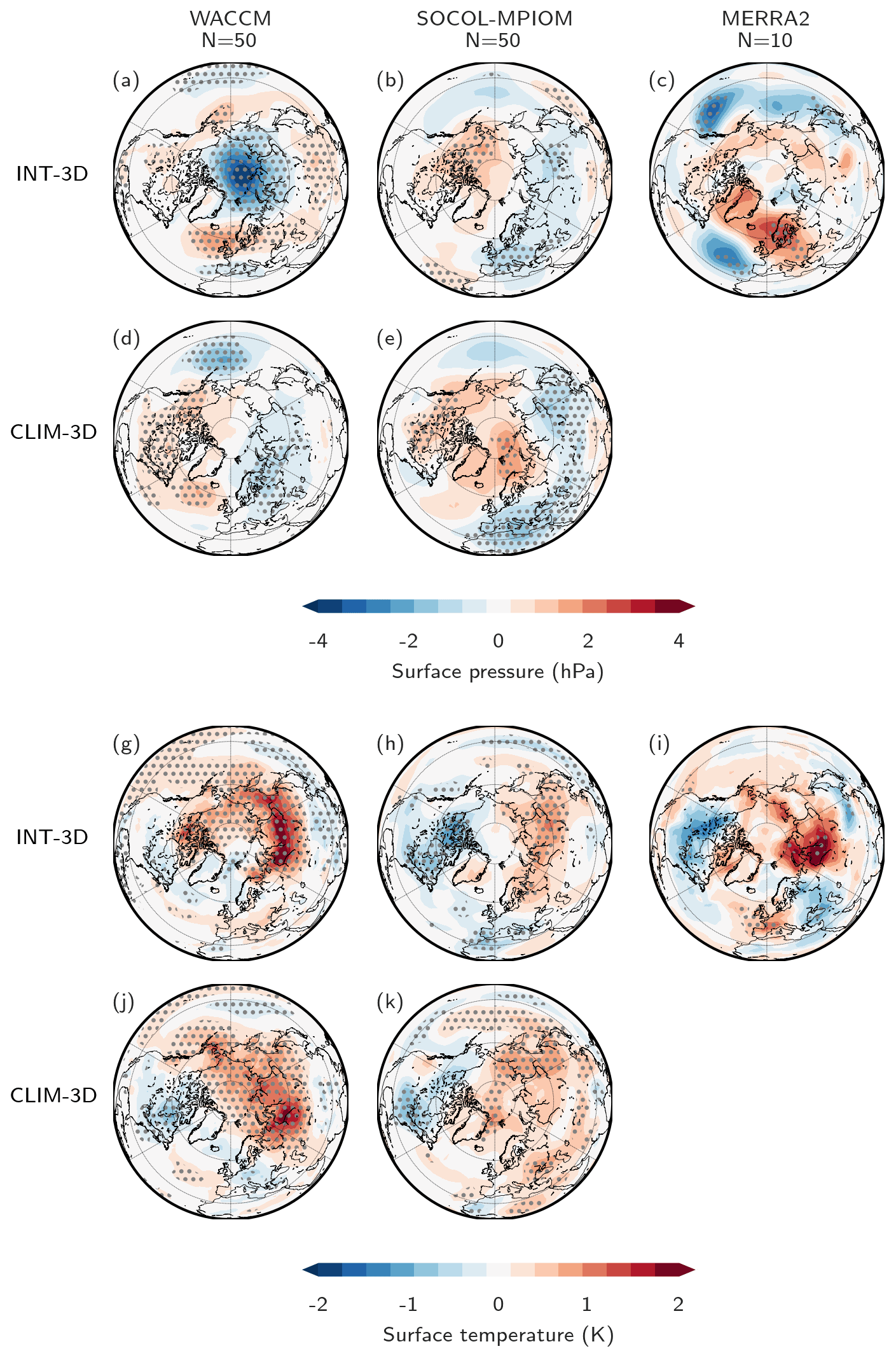
Figure 5The surface impact of FSWs in low-ozone springs and the impact of ozone. SLP (a–e) and temperature (f–j) anomalies in the month after the 50 hPa FSW in low-ozone springs for WACCM INT-3D (a, f), SOCOL-MPIOM INT-3D (b, g), MERRA2 (c, h), WACCM CLIM-3D (d, i), and SOCOL-MPIOM CLIM-3D (e, j). Stippling shows significance on a 4.6 % level (2σ) following a bootstrapping test.
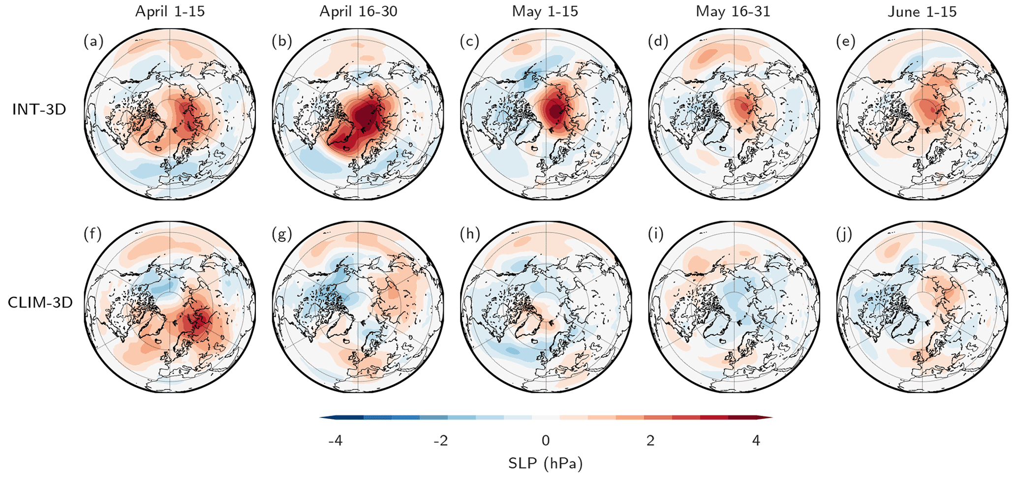
Figure 6Seasonal evolution of SLP anomalies in high-ozone years in WACCM. Evolution of SLP anomalies from April to June in high-ozone springs in WACCM simulations with interactive ozone chemistry (a–e) and climatological ozone (f–j). The mean ozone maximum date in INT-3D simulations is March 7, while the mean FSW date is 17 April.
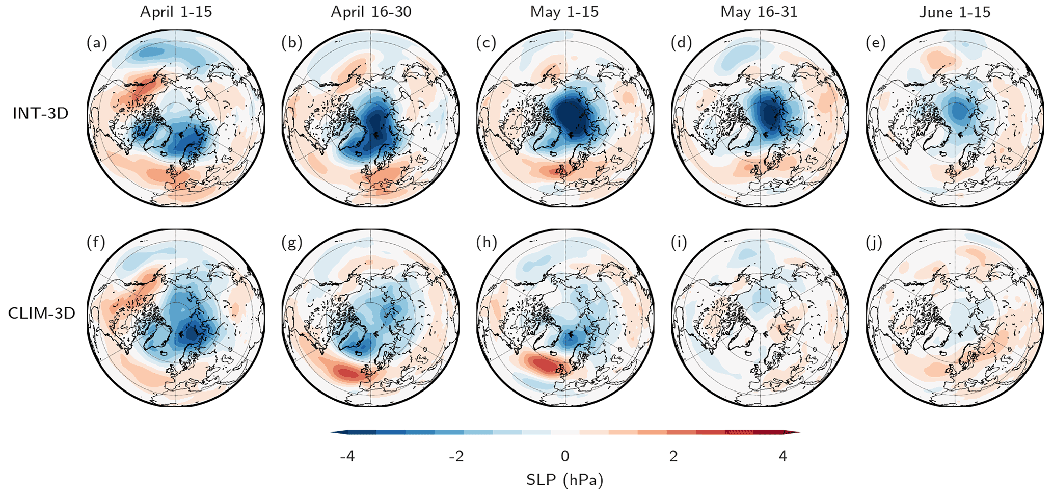
Figure 7Seasonal evolution of SLP anomalies in low-ozone years in WACCM. Evolution of SLP anomalies from April to June in low-ozone springs in WACCM simulations with interactive ozone chemistry (a–e) and climatological ozone (f–j). The mean ozone minimum date in INT-3D simulations is 20 April, while the mean FSW date is 10 May.
3.3 Ozone feedback mechanism
After having quantified the impact of ozone on the timing and surface response of FSW, we explain the mechanism by which ozone modulates the FSW and its downward coupling. Briefly, we will demonstrate that high- and low-ozone levels are associated with weak and strong polar vortex states, respectively. In the lower stratosphere, the anomalous vortex states are significantly strengthened by ozone anomalies as they affect shortwave heating and planetary wave propagation, leading to a shift of the timing of the vortex breakup towards earlier and later dates in high- and low-ozone springs, respectively.
We start by focusing on the 25 % of springs with the largest Arctic stratospheric ozone abundances. In both sets of simulations and the reanalysis, the FSW in high-ozone springs is early below and delayed above ∼ 10 hPa. Before describing the ozone impacts on the FSW, we first explain the origin of this vertical dipole structure in the timing of the FSW. As shown in Fig. A1, the zonal mean zonal wind at 50 hPa in high-ozone springs (red lines) is already weaker than on average in March in all model simulations and reanalysis and eventually breaks up early. Weak westerly winds in the lower stratosphere in high-ozone springs, as seen in Fig. A1 (red lines), are consistent with our understanding of the processes that drive the ozone maxima: increased planetary wave driving, which decelerates the polar vortex, goes along with a strengthening of the Brewer–Dobson circulation and thus an increased transport of ozone-rich air from lower latitudes to the polar region (Salby and Callaghan, 2007; Tegtmeier et al., 2008). Additionally, warm temperatures associated with the weak vortex inhibit the formation of polar stratospheric clouds (PSCs), and chemical ozone depletion is suppressed (Salby and Callaghan, 2007). Hence, weak polar vortices typically result in high ozone concentrations over the pole. The weaker than usual polar vortex in the lower stratosphere in high-ozone springs has consequences on the upper stratosphere; weak westerlies around the FSW inhibit planetary wave propagation to the upper stratosphere, where westerly winds are thus unperturbed and the FSW at these levels is delayed, as seen in Fig. 2 (red lines). This mechanism leads to opposite effects on the timing of the FSW in the upper and lower stratosphere in high-ozone springs, resulting in an early FSW at low and delayed FSW at high altitudes and thus a FSW which is more similar to 10 hPa-first (Hardiman et al., 2011). This result is consistent with previous findings stating that the vertical evolution of the FSW is sensitive to the polar vortex state, with weak polar vortices being linked to 10 hPa-first FSW (Hardiman et al., 2011).
In low-ozone springs, an opposite mechanism is in place; low ozone concentrations are correlated with a strong polar vortex, which inhibits transport of ozone from the tropics and sets the basis for cold stratospheric temperatures and subsequent formation of PSCs, leading to heterogeneous chlorine activation and subsequent ozone depletion (Solomon, 1999). Just as in high-ozone springs, the pattern of the FSW date in the upper and lower stratosphere is opposite, although the signal in the upper stratosphere in WACCM and MERRA2 is not as pronounced as in high-ozone springs. A strong polar vortex in the lower stratosphere around the FSW in low-ozone springs is accompanied by weak winds at higher altitudes due to increased wave guiding to that region. These processes lead to an early FSW date below ∼ 10 hPa in all model simulations and reanalysis (see Fig. 2). Therefore, the vertical structure of FSWs in low-ozone springs is more like 1 hPa-first.
Ozone perturbations resulting from the weak or strong polar vortex in high- and low-ozone years in turn affect stratospheric dynamics via their impact on radiative heating (see Fig. A6). In the case of high-ozone springs, ozone anomalies lead to a large absorption of solar radiation in the stratosphere when sunlight returns to the pole in spring, (see Fig. 8d, i), which results in additional heating. This heating decreases the meridional temperature gradient, and the polar vortex strength decreases accordingly, leading to further weakening of the winds. The evolution of the vortex for both sets of experiments in high-ozone springs is depicted in Fig. 8a, b and f, g. By comparing the absolute zonal wind in INT-3D and CLIM-3D, we see that while both experiments show weak winds and an early FSW in the lower stratosphere in high-ozone springs in both models (see Fig. A1, red lines), zonal mean zonal wind decreases faster in INT-3D due to additional heating by ozone in both models (see Fig. 8 c, h), resulting in an even earlier FSW (see also Fig. A1 solid vs. stippled lines). Starting from around end of April, the ozone-induced vortex weakening reaches the troposphere, where it significantly impacts surface climate, as shown previously (see Figs. 8 c, h; 4).
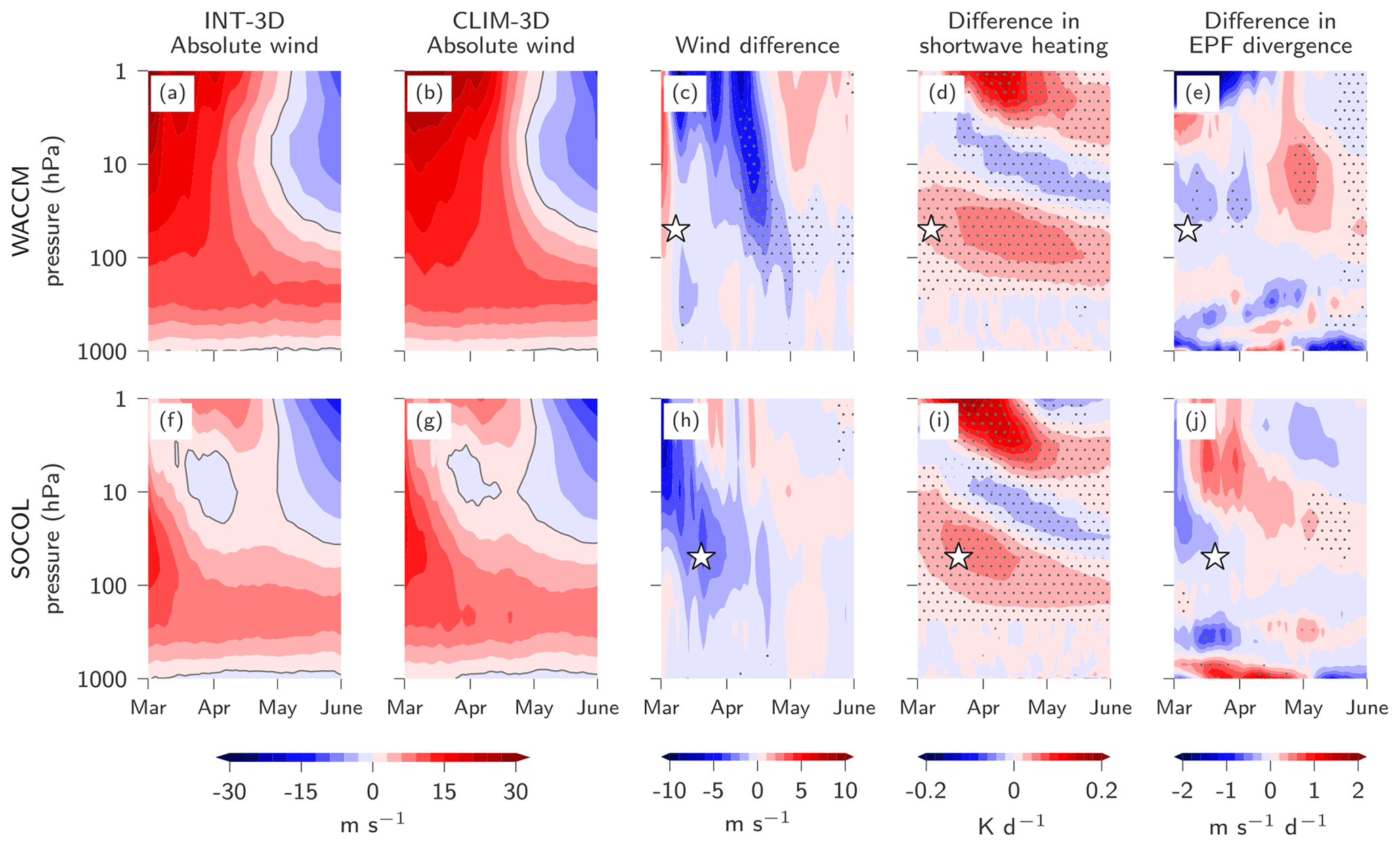
Figure 8The impact of ozone anomalies on zonal wind and wave breaking in high-ozone springs. WACCM (top row) and SOCOL-MPIOM (bottom row) 55–75∘ N zonal mean zonal wind in high-ozone springs in INT-3D (first column) and CLIM-3D (second column) and zonal mean zonal wind in INT-3D minus CLIM-3D (third column). Differences in shortwave heating anomalies between INT-3D and CLIM-3D (d, i) and differences in EPF divergence between INT-3D and CLIM-3D (30 d running mean, right column). The ozone maximum date is marked by a star. Stippling shows regions where differences between INT-3D and CLIM-3D are significant on a 4.6 % level.
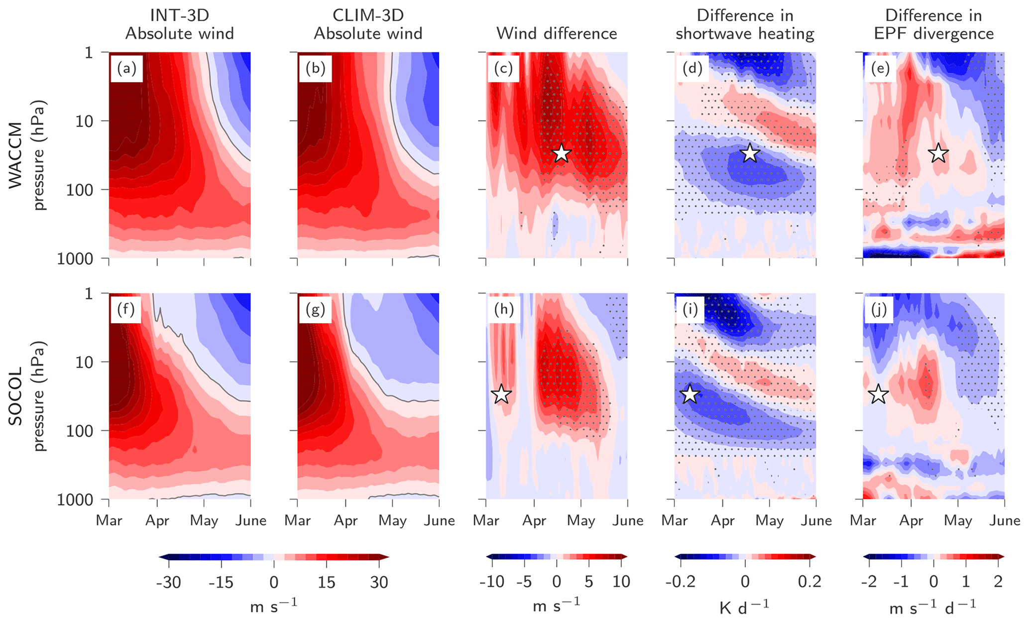
Figure 9The impact of ozone anomalies on zonal wind and wave breaking in low-ozone springs. WACCM (top row) and SOCOL-MPIOM (bottom row) 55–75∘ N zonal mean zonal wind in low-ozone springs in INT-3D (first column) and CLIM-3D (second column) and zonal mean zonal wind in INT-3D minus CLIM-3D (third column). Differences in shortwave heating anomalies between INT-3D and CLIM-3D (d, i) and differences in EPF divergence between INT-3D and CLIM-3D (30 d running mean, right column). The ozone minimum date is marked by a star. Stippling shows regions where differences between INT-3D and CLIM-3D are significant on a 4.6 % level.
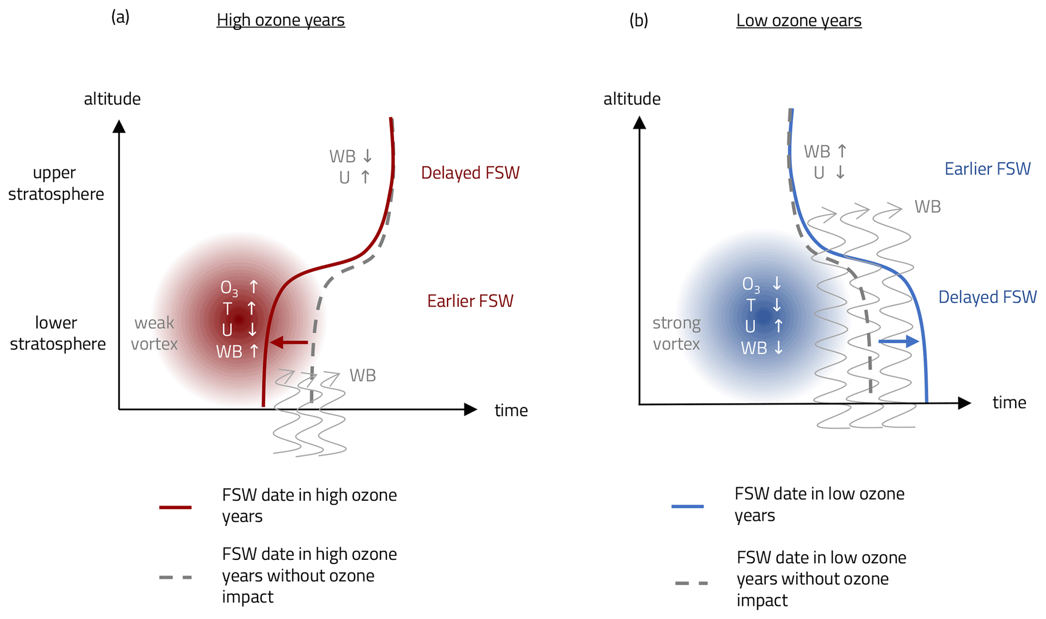
Figure 10Ozone feedback mechanism around the FSW date. Dashed grey lines indicate the dipole structure of the FSW date without ozone impact (as in the CLIM-3D setting), i.e., merely as a result of a weak or strong polar vortex and subsequent implications for wave breaking (WB) in the upper stratosphere. Impacts of ozone anomalies on temperature (T), zonal wind (U) and WB acting on top of the dynamical processes around the FSW date are highlighted in red (a) and in blue (b) for low- and high-ozone years, respectively. The red and blue arrows show the subsequent shift in the timing of the FSW induced by ozone. The resulting FSW date is schematically shown by the thick red line (high-ozone springs) and the thick blue line (low-ozone springs).
In addition to these processes, the weakening of the polar vortex by ozone in high-ozone springs has further implications for planetary wave propagation. Around the onset of the FSW, when the westerly winds are weak, further deceleration of westerly winds in the lower stratosphere by ozone leads to a dissipation of planetary waves already at lower altitudes, amplifying the heating due to radiative processes (shortwave absorption). As the propagation of planetary waves through the stratosphere is thereby reduced, less wave dissipation takes place in the upper stratosphere, where zonal winds are thereby enhanced. This mechanism is analogous to the “negative feedback” described in Haase and Matthes (2019). The enhanced wave dissipation in the upper stratosphere compensates for the shortwave heating effects in this region, meaning that feedbacks arising from the coupling between ozone and the circulation do not significantly affect the timing of the FSW in the upper stratosphere (see Fig. 2 INT-3D vs. CLIM-3D). Rather, ozone anomalies shift the FSW below ∼ 10 hPa to earlier dates (via the impacts on shortwave heating and planetary wave breaking). Most remarkably, this pattern is robust across both models. A schematic representation of the driving processes is shown in Fig. 10a.
In low-ozone springs, the two-way coupling between ozone and the circulation is analogous to that in high-ozone springs. Figure 9 shows the impact of low ozone concentrations on the polar vortex strength by comparing zonal mean zonal wind in INT-3D and CLIM-3D simulations. Ozone anomalies in INT-3D strengthen the polar vortex throughout the stratosphere (Fig. 9c, h) due to a decrease in shortwave heating by ozone (Fig. 9d, i). Thus, winter conditions in the stratosphere are extended and the FSW at lower altitudes is clearly delayed, as shown in Fig. 2. As in high-ozone springs, the modulation of the FSW timing by ozone is largest in the lower stratosphere (50 hPa). Thus, the ozone–dynamics coupling makes FSWs predominantly like 1 hPa-first.
For both high- and low-ozone years it is important to highlight that the zonal winds in the beginning of March are of the same strength in both INT-3D and CLIM-3D experiments and only differ in spring when sunlight returns to the polar cap and ozone perturbations can affect temperature via shortwave heating (Fig. A1), indicating that the background conditions in INT-3D and CLIM-3D are comparable.
While previous studies have linked the stratospheric background state (weak and strong polar vortex) to either the timing or the vertical structure of the FSW (see, e.g., Waugh et al., 1999; Hardiman et al., 2011), here we go one step further by establishing a connection between the vertical structure of the FSW, its timing, preceding stratospheric anomalies, and stratospheric ozone. In summary, a holistic examination of the processes at work reveals, for the first time, that in high-ozone springs a weak polar vortex tends to be followed by a 10 hPa-first FSW with an early FSW date below ∼ 10 hPa. Both the vertical structure and the timing of the FSW are thereby to a large part driven by ozone. By influencing the timing and the vertical structure of FSWs (i.e., making them more “sudden”), ozone also amplifies the surface signature of FSWs in high-ozone springs. In turn, in low-ozone springs, we find a strong polar vortex and a delayed vortex breakup below ∼ 10 hPa and a vertical structure which is more like 1 hPa-first. Again, both the timing and the vertical structure of the FSW are thereby largely a result of the low ozone concentrations.
It is well known that stratospheric ozone responds to circulation anomalies and is thus an indicator of the dynamical state of the stratosphere. For example, enhanced planetary wave forcing in the Arctic spring may lead not only to an early breakup of the stratospheric polar vortex but also to ozone-rich conditions over the pole due to increased import of ozone from lower latitudes (Salby and Callaghan, 2007). The reduction of such wave forcing, in turn, results in a delayed final stratospheric warming (FSW) and persistent low ozone in the stratosphere. However, here we show with two independent chemistry–climate models that ozone not only reacts to the dynamical conditions which determine the timing of the FSW (like a passive tracer) but also actively modulates its timing and downward impact through ozone–dynamics coupling. More specifically, our results allow us to draw the following conclusions.
-
Stratospheric ozone significantly impacts the timing of the FSW in the middle and lower stratosphere below 10 hPa. In years with high ozone concentrations, the FSW is advanced even further (up to 10 d) by the feedback resulting from the mutual coupling between ozone and circulation. In ozone-deficient years, on the contrary, ozone prolongs winter conditions in the stratosphere and delays the breakup of the polar vortex by more than 10 d. Thus, stratospheric ozone anomalies significantly increase the variability in the timing of the FSW.
-
Ozone modulates not only the timing of FSWs but also their downward impact. More specifically, FSWs in high-ozone springs are followed by positive sea level pressure (SLP) anomalies centered around the pole and cooling over much of Eurasia and Europe. These anomalies are substantially (to at least 50 %) driven by ozone. While these surface effects are robust in high-ozone springs across the two models examined here, ozone has no significant effect on the already negligible surface response of FSW in springs with strong ozone depletion.
-
Ozone modulates the evolution and downward coupling of FSW via effects on shortwave heating and wave driving. In years with high ozone concentrations, greater absorption of UV light by ozone leads to stratospheric warming and a weakening of the polar vortex, allowing enhanced propagation of planetary waves into the stratosphere, which further weakens the westerly winds and leads to earlier FSW. In years with strong ozone depletion, the reduced UV absorption in the stratosphere leads to cooling and a strengthening of the polar vortex, allowing for fewer waves to propagate through the stratosphere. Reduced wave breaking and shortwave heating under ozone-depleted conditions lead to a strong vortex, which lasts until late spring, resulting in a late FSW.
Ozone anomalies develop gradually throughout the season and become apparent as early as late winter (see Fig. A2). Given the close relationship between ozone and the FSW, ozone anomalies could serve as a predictor of the late or early timing of the FSW expected in the lower stratosphere. Moreover, our results show that the inclusion of interactive ozone chemistry in climate models improves the representation of springtime surface climate. Therefore, stratospheric ozone is potentially of value for subseasonal to seasonal prediction. Our results further suggest that interactive ozone is important in capturing the variability in the timing of FSWs and their effects on surface climate in spring. Explorations of ways to incorporate ozone–dynamics coupling into weather and climate models will be beneficial for improvements in subseasonal to seasonal forecasts.
In the Southern Hemisphere, ozone depletion has cooled the polar stratosphere since the late 1970s (Randel et al., 2009), having led to an overall delay of the FSW (Waugh et al., 1999; Sun et al., 2014; Rao and Garfinkel, 2021a). While there is no robust evidence for long-term trends in the timing of the Arctic FSW due to large interannual variability, a similar tendency towards a delay of FSWs caused by ozone depletion has been suggested (Waugh et al., 1999; Thiéblemont et al., 2019; Rao and Garfinkel, 2021a). With ozone-depleting substances being phased out after the adoption of the Montreal Protocol and its amendments, polar total ozone column is expected to recover to 1980 levels (Strahan and Douglass, 2018). The polar stratosphere is therefore expected to warm, especially in the Southern Hemisphere, where the trend in ozone is more pronounced. However, rising greenhouse gas concentrations increasingly cool the stratosphere, competing with ozone-induced warming (Pisoft et al., 2021). It is therefore unclear how the timing of the FSW will evolve in the future, but it has been suggested that there might be a trend towards delayed FSWs in both hemispheres in high-emission scenarios – despite the expected ozone recovery (Rao and Garfinkel, 2021a). Given the potential ability of ozone in influencing seasonal and long-term climate in both the stratosphere and troposphere, further work is needed to investigate the importance of interactive ozone chemistry for spring climate under future conditions and to disentangle the effects of elevated greenhouse gas and ozone concentrations on the lifetime of the stratospheric polar vortex.
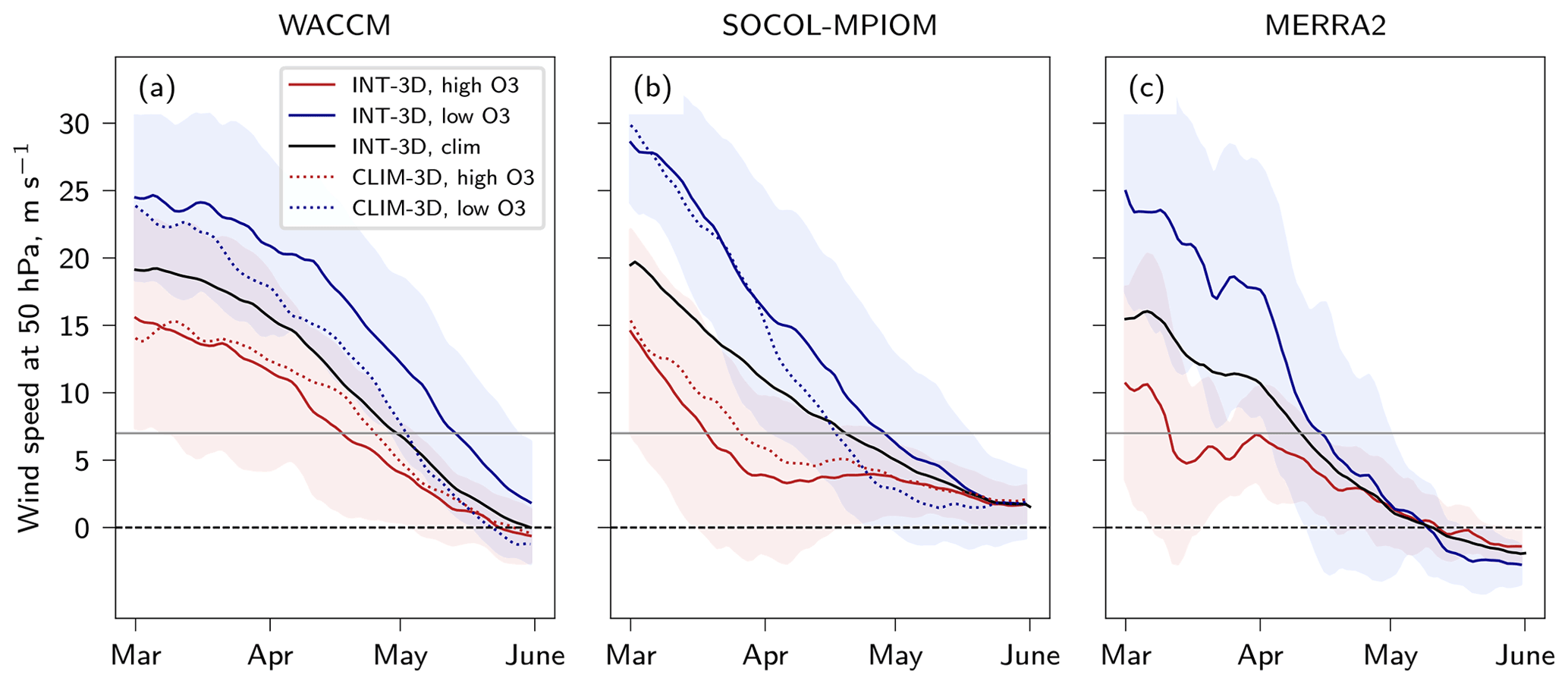
Figure A1Zonal wind evolution in high- and low-ozone springs. Zonal mean zonal wind at 50 hPa averaged between 55 and 75∘ N in high-ozone (red) and low-ozone (blue) springs in INT-3D (solid line) and CLIM-3D (stippled line) and the wind climatology (black) in (a) WACCM and (b) SOCOL-MPIOM as well as in (c) MERRA2. The grey line indicates the wind threshold of 7 m s−1 used to define the FSW date at 50 hPa. Shaded areas show the standard deviation in high- and low-ozone springs in INT-3D simulations.

Figure A2Ozone evolution in high- and low-ozone years. Evolution of ozone over the year in the 25 % of years with the lowest (blue) and highest (red) springtime partial ozone column values between 30 and 70 hPa in (a) WACCM INT-3D, (b) SOCOL-MPIOM INT-3D, and (c) MERRA2. The grey line shows the climatology over all years in the respective datasets (200 years for WACCM and SOCOL-MPIOM and 41 years for MERRA2). Shaded areas show the standard deviation across high- and low-ozone years.
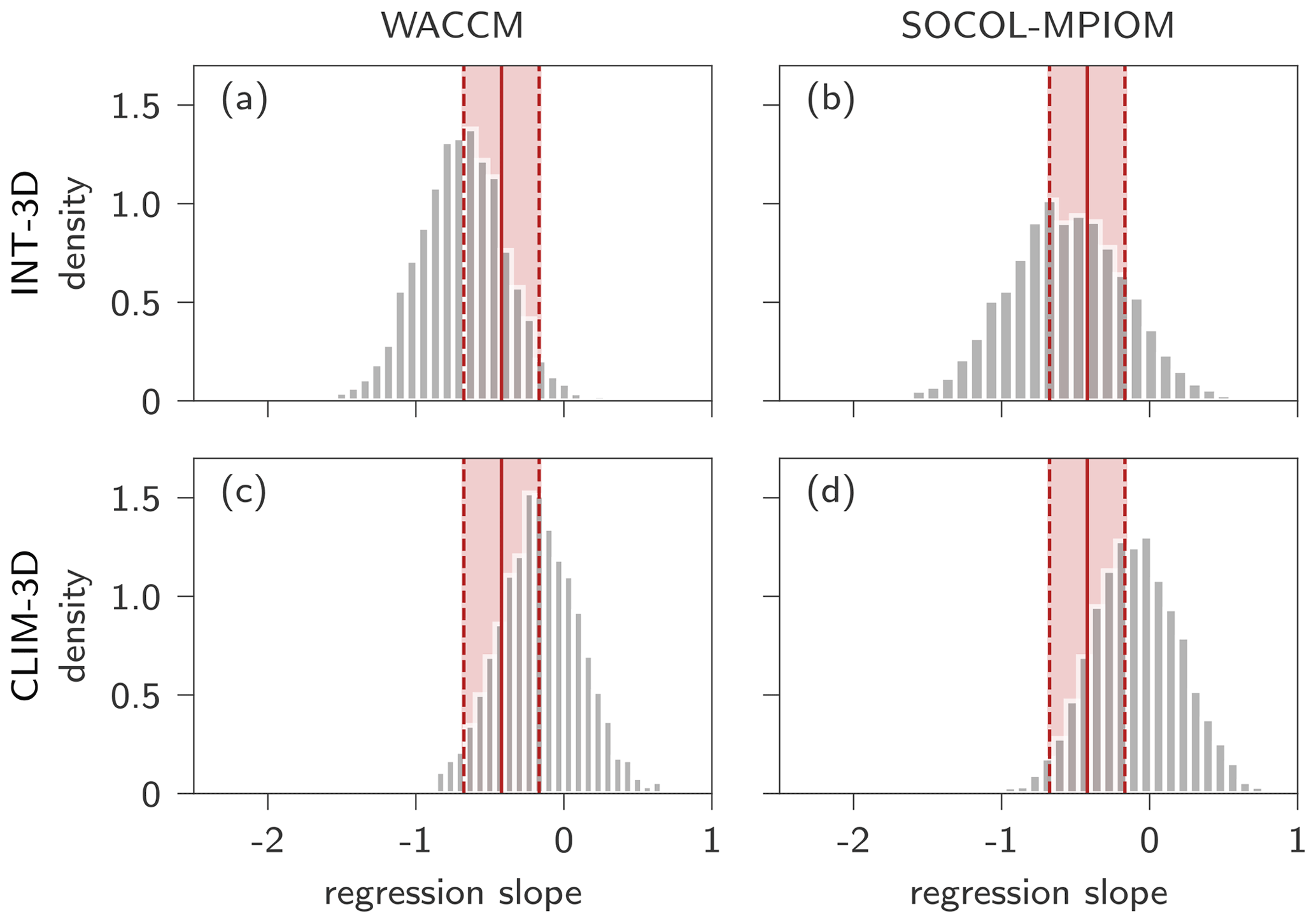
Figure A3Regression slopes in model simulations and reanalysis. Regression slope of the maximum 5 d running mean partial ozone column (30–70 hPa) on the FSW date following Fig. 3 for 5000 samples consisting of 40 randomly selected years each for both sets of model simulations. The regression slope of the reanalysis is shown by the solid red line, with its standard error indicated by the red shaded area.

Figure A4AO evolution in high- and low-ozone springs. Evolution of the Arctic Oscillation in the 25 % of springs with the lowest (blue) and highest (red) ozone concentrations in WACCM (first column) and SOCOL-MPIOM (second column) in INT-3D (a, b) and CLIM-3D (c, d). Dots mark days where the AO is significantly different from zero on a 5 % level based on a Student's t test. Shaded areas show the standard deviation across high- and low-ozone years. Circles mark mean ozone maximum and minimum dates and mean FSW dates in high- and low-ozone springs.
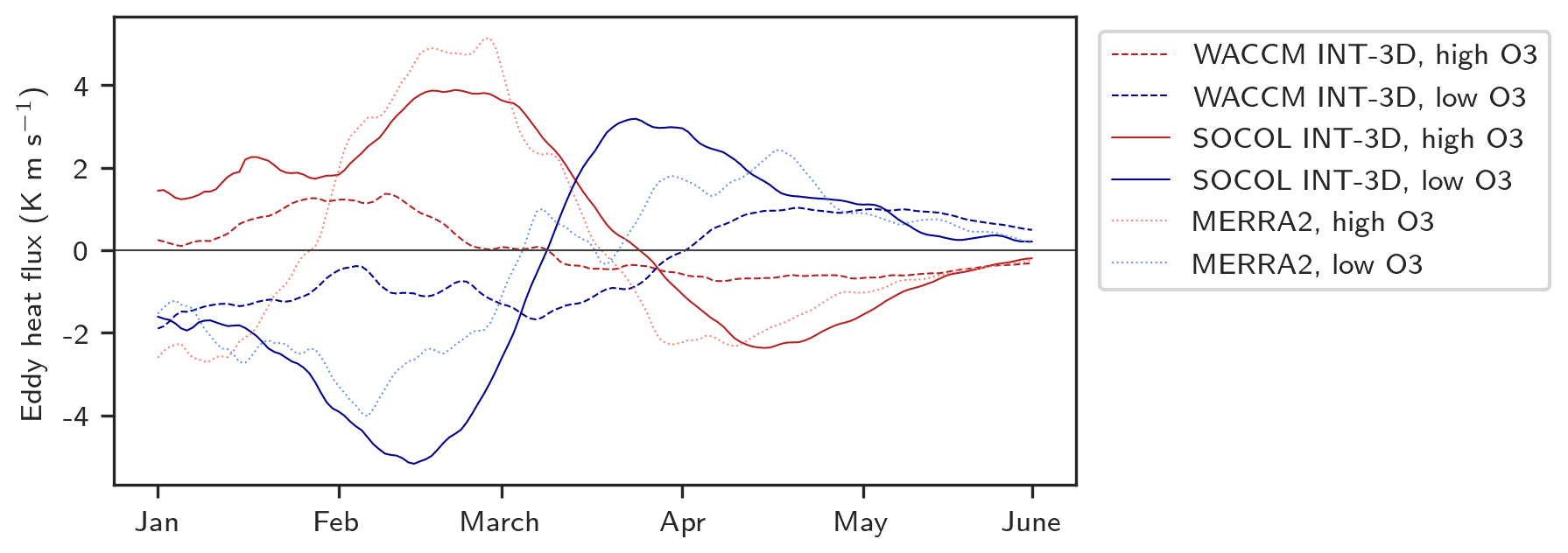
Figure A5Heat flux at 100 hPa in high- and low-ozone springs. Eddy heat flux anomalies (K m s−1, 30 d running mean) averaged over 45–75∘ N at 100 hPa for high- and low-ozone springs for WACCM and SOCOL-MPIOM INT-3D simulations and for MERRA2.

Figure A6Ozone and shortwave heating anomalies in high- and low-ozone springs. Ozone anomalies in experiments with interactive ozone chemistry in low-ozone (a, e) and high-ozone (c, g) springs and differences in shortwave heating anomalies between INT-3D and CLIM-3D in low-ozone (b, f) and high-ozone (d, h) springs in WACCM (a–d) and SOCOL-MPIOM (e–h).
All code and scripts used for the analysis in this study are available from the corresponding author upon reasonable request. The modeling data used in this study is available in the ETH Research Collection. Data for WACCM are available at https://doi.org/10.3929/ethz-b-000527155 (Friedel and Chiodo, 2022b). Data for SOCOL-MPIOM are available at https://doi.org/10.3929/ethz-b-000546039 (Friedel and Chiodo, 2022a).
The MERRA2 reanalysis data can be downloaded from the Goddard Earth Sciences Data and Information Services Center (GES DIC) (https://disc.gsfc.nasa.gov/datasets/M2I3NPASM_5.12.4/summary?keywords=MERRA2, last access: 20 October 2021; https://doi.org/10.5067/QBZ6MG944HW0, GMAO, 2015).
GC conceived the modeling experiments. GC, MF, and AS conducted the modeling experiments. MF and GC processed the data. MF, GC, TP, and DIVD analyzed and interpreted the results. MF wrote the paper with input from all authors.
The contact author has declared that none of the authors has any competing interests.
Publisher's note: Copernicus Publications remains neutral with regard to jurisdictional claims in published maps and institutional affiliations.
We are grateful for the assistance from Urs Beyerle in data management.
This research has been supported by the Swiss National Science Foundation through Ambizione grant no. PZ00P2_180043 to Marina Friedel and Gabriel Chiodo and through project PP00P2_198896 to Daniela I. V. Domeisen.
This paper was edited by Farahnaz Khosrawi and reviewed by two anonymous referees.
Andrews, D. G. and McIntyre, M. E.: Planetary waves in horizontal and vertical shear: The generalized Eliassen-Palm relation and the mean zonal acceleration, J. Atmos. Sci., 33, 2031–2048, https://doi.org/10.1175/1520-0469(1976)033<2031:PWIHAV>2.0.CO;2, 1976. a
Andrews, D. G., Holton, J. R., and Leovy, C. B.: Middle atmosphere dynamics, Academics, San Diego, California, USA, 1987. a
Ayarzagüena, B. and Serrano, E.: Monthly characterization of the tropospheric circulation over the Euro-Atlantic Area in Relation with the Timing of Stratospheric Final Warmings, J. Climate, 22, 6313–6324, https://doi.org/10.1175/2009JCLI2913.1, 2009. a, b, c, d
Bahramvash Shams, S., Walden, V. P., Hannigan, J. W., Randel, W. J., Petropavlovskikh, I. V., Butler, A. H., and de la Cámara, A.: Analyzing ozone variations and uncertainties at high latitudes during sudden stratospheric warming events using MERRA-2, Atmospheric Chemistry and Physics, 22, 5435–5458, https://doi.org/10.5194/acp-22-5435-2022, 2022. a, b
Baldwin, M. P. and Dunkerton, T. J.: Stratospheric harbingers of anomalous weather regimes, Science, 294, 581–584, https://doi.org/10.1126/science.1063315, 2001. a, b
Baldwin, M. P. and Thompson, D. W.: A critical comparison of stratosphere–troposphere coupling indices, Q. J. Roy. Meteor. Soc., 135, 1661–1672, https://doi.org/10.1002/qj.479, 2009. a
Baldwin, M. P., Ayarzagüena, B., Birner, T., Butchart, N., Butler, A. H., Charlton-Perez, A. J., Domeisen, D. I. V., Garfinkel, C. I., Garny, H., Gerber, E. P., Hegglin, M. I., Langematz, U., and Pedatella, N. M.: Sudden Stratospheric Warmings, Rev. Geophys., 59, e2020RG000708, https://doi.org/10.1029/2020RG000708, 2021. a
Bergner, N., Friedel, M., Domeisen, D. I. V., Waugh, D., and Chiodo, G.: Exploring the link between austral stratospheric polar vortex anomalies and surface climate in chemistry-climate models, Atmos. Chem. Phys., 22, 13915–13934, https://doi.org/10.5194/acp-22-13915-2022, 2022. a
Black, R. X. and McDaniel, B. A.: The dynamics of Northern Hemisphere stratospheric final warming events, J. Atmos. Sci., 64, 2932–2946, https://doi.org/10.1175/JAS3981.1, 2007a. a
Black, R. X. and McDaniel, B. A.: Interannual variability in the Southern Hemisphere circulation organized by stratospheric final warming events, J. Atmos. Sci., 64, 2968–2974, https://doi.org/10.1175/JAS3979.1, 2007b. a
Black, R. X., McDaniel, B. A., and Robinson, W. A.: Stratosphere–troposphere coupling during spring onset, J. Climate, 19, 4891–4901, https://doi.org/10.1175/JCLI3907.1, 2006. a, b, c, d, e, f, g
Butchart, N., Charlton-Perez, A. J., Cionni, I., Hardiman, S. C., Haynes, P. H., Krüger, K., Kushner, P. J., Newman, P. A., Osprey, S. M., Perlwitz, J., Sigmond, M., Wang, L., Akiyoshi, H., Austin, J., Bekki, S., Baumgaertner, A., Braesicke, P., Brühl, C., Chipperfield, M., Dameris, M., Dhomse, S., Eyring, V., Garcia, R., Garny, H., Jöckel, P., Lamarque, J.-F., Marchand, M., Michou, M., Morgenstern, O., Nakamura, T., Pawson, S., Plummer, D., Pyle, J., Rozanov, E., Scinocca, J., Shepherd, T. G., Shibata, K., Smale, D., Teyssèdre, H., Tian, W., Waugh, D., and Yamashita, Y.: Multimodel climate and variability of the stratosphere, J. Geophys. Res.-Atmos., 116, D05102, https://doi.org/10.1029/2010JD014995, 2011. a, b
Butler, A. H. and Domeisen, D. I. V.: The wave geometry of final stratospheric warming events, Weather and Climate Dynamics, 2, 453–474, https://doi.org/10.5194/wcd-2-453-2021, 2021. a, b
Butler, A. H., Charlton-Perez, A., Domeisen, D. I., Simpson, I. R., and Sjoberg, J.: Predictability of Northern Hemisphere final stratospheric warmings and their surface impacts, Geophys. Res. Lett., 46, 10578–10588, https://doi.org/10.1029/2019GL083346, 2019. a, b
Cionni, I., Eyring, V., Lamarque, J. F., Randel, W. J., Stevenson, D. S., Wu, F., Bodeker, G. E., Shepherd, T. G., Shindell, D. T., and Waugh, D. W.: Ozone database in support of CMIP5 simulations: results and corresponding radiative forcing, Atmos. Chem. Phys., 11, 11267–11292, https://doi.org/10.5194/acp-11-11267-2011, 2011. a
Danabasoglu, G., Bates, S. C., Briegleb, B. P., Jayne, S. R., Jochum, M., Large, W. G., Peacock, S., and Yeager, S. G.: The CCSM4 ocean component, J. Climate, 25, 1361–1389, https://doi.org/10.1175/JCLI-D-11-00091.1, 2012. a
Davis, S. M., Hegglin, M. I., Fujiwara, M., Dragani, R., Harada, Y., Kobayashi, C., Long, C., Manney, G. L., Nash, E. R., Potter, G. L., Tegtmeier, S., Wang, T., Wargan, K., and Wright, J. S.: Assessment of upper tropospheric and stratospheric water vapor and ozone in reanalyses as part of S-RIP, Atmos. Chem. Phys., 17, 12743–12778, https://doi.org/10.5194/acp-17-12743-2017, 2017. a
Egorova, T., Rozanov, E., Zubov, V., and Karol, I.: Model for investigating ozone trends (MEZON), Izvestiya – Atmospheric and Ocean Physics, 39, 277–292, 2003. a
Eyring, V., Arblaster, J. M., Cionni, I., Sedláček, J., Perlwitz, J., Young, P. J., Bekki, S., Bergmann, D., Cameron-Smith, P., Collins, W. J., Faluvegi, G., Gottschaldt, K.-D., Horowitz, L. W., Kinnison, D. E., Lamarque, J.-F., Marsh, D. R., Saint-Martin, D., Shindell, D. T., Sudo, K., Szopa, S., and Watanabe, S.: Long-term ozone changes and associated climate impacts in CMIP5 simulations, J. Geophys. Res.-Atmos., 118, 5029–5060, https://doi.org/10.1002/jgrd.50316, 2013. a
Friedel, M. and Chiodo, G.: Model results for “Robust effect of springtime Arctic ozone depletion on surface climate”, part 2. Data for SOCOL-MPIOM, ETH Zürich [data set], https://doi.org/10.3929/ethz-b-000546039, 2022a. a
Friedel, M. and Chiodo, G.: Model results for “Robust effect of springtime Arctic ozone depletion on surface climate”, ETH Zürich [data set], https://doi.org/10.3929/ethz-b-000527155, 2022b. a
Friedel, M., Chiodo, G., Stenke, A., Domeisen, D. I., Fueglistaler, S., Anet, J., and Peter, T.: Springtime Arctic ozone depletion forces Northern Hemisphere climate anomalies, Nat. Geosci., in press, 2022. a, b, c, d, e, f, g, h, i, j, k, l, m
Gelaro, R., McCarty, W., Suárez, M. J., Todling, R., Molod, A., Takacs, L., Randles, C. A., Darmenov, A., Bosilovich, M. G., Reichle, R., Wargan, K., Coy, L., Cullather, R., Draper, C., Akella, S., Buchard, V., Conaty, A., da Silva, A. M., Gu, W., Kim, G.-K., Koster, R., Lucchesi, R., Merkova, D., Nielsen, J. E., Partyka, G., Pawson, S., Putman, W., Rienecker, M., Schubert, S. D., Sienkiewicz, M., and Zhao, B.: The Modern-Era Retrospective Analysis for Research and Applications, Version 2 (MERRA-2), J. Climate, 30, 5419–5454, https://doi.org/10.1175/JCLI-D-16-0758.1, 2017. a
GMAO (Global Modeling and Assimilation Office): MERRA-2 inst3_3d_asm_Np: 3d,3-Hourly,Instantaneous,Pressure-Level,Assimilation,Assimilated Meteorological Fields V5.12.4, Greenbelt, MD, USA, Goddard Earth Sciences Data and Information Services Center (GES DISC) [data set], https://doi.org/10.5067/QBZ6MG944HW0, 2015. a
Haase, S. and Matthes, K.: The importance of interactive chemistry for stratosphere–troposphere coupling, Atmos. Chem. Phys., 19, 3417–3432, https://doi.org/10.5194/acp-19-3417-2019, 2019. a, b, c, d, e, f, g, h
Hardiman, S. C., Butchart, N., Charlton-Perez, A. J., Shaw, T. A., Akiyoshi, H., Baumgaertner, A., Bekki, S., Braesicke, P., Chipperfield, M., Dameris, M., Garcia, R. R., Michou, M., Pawson, S., Rozanov, E., and Shibata, K.: Improved predictability of the troposphere using stratospheric final warmings, J. Geophys. Res.-Atmos., 116, D18113, https://doi.org/10.1029/2011JD015914, 2011. a, b, c, d, e, f, g
Hendon, H. H., Lim, E.-P., and Abhik, S.: Impact of interannual ozone variations on the downward coupling of the 2002 Southern Hemisphere stratospheric warming, J. Geophys. Res.-Atmos., 125, e2020JD032952, https://doi.org/10.1029/2020JD032952, 2020. a
Hersbach, H., Bell, B., Berrisford, P., Hirahara, S., Horányi, A., Muñoz-Sabater, J., Nicolas, J., Peubey, C., Radu, R., Schepers, D., Simmons, A., Soci, C., Abdalla, S., Abellan, X., Balsamo, G., Bechtold, P., Biavati, G., Bidlot, J., Bonavita, M., De Chiara, G., Dahlgren, P., Dee, D., Diamantakis, M., Dragani, R., Flemming, J., Forbes, R., Fuentes, M., Geer, A., Haimberger, L., Healy, S., Hogan, R. J., Hólm, E., Janisková, M., Keeley, S., Laloyaux, P., Lopez, P., Lupu, C., Radnoti, G., de Rosnay, P., Rozum, I., Vamborg, F., Villaume, S., and Thépaut, J.-N.: The ERA5 global reanalysis, Q. J. Roy. Meteor. Soc., 146, 1999–2049, https://doi.org/10.1002/qj.3803, 2020. a
Holland, M. M., Bailey, D. A., Briegleb, B. P., Light, B., and Hunke, E.: Improved sea ice shortwave radiation physics in CCSM4: The impact of melt ponds and aerosols on Arctic sea ice, J. Climate, 25, 1413–1430, https://doi.org/10.1175/JCLI-D-11-00078.1, 2012. a
Hu, J., Ren, R., and Xu, H.: Occurrence of winter stratospheric sudden warming events and the seasonal timing of spring stratospheric final warming, J. Atmos. Sci., 71, 2319–2334, https://doi.org/10.1175/JAS-D-13-0349.1, 2014. a, b, c
Jinggao, H., Ren, R., Yu, Y., and Xu, H.: The boreal spring stratospheric final warming and its interannual and interdecadal variability, Sci. China Earth Sci., 57, 710–718, https://doi.org/10.1007/s11430-013-4699-x, 2013. a
Kelleher, M. E., Ayarzagüena, B., and Screen, J. A.: Interseasonal connections between the timing of the stratospheric final warming and Arctic sea ice, J. Climate, 33, 3079–3092, https://doi.org/10.1175/JCLI-D-19-0064.1, 2020. a
Lawrence, Z. D., Perlwitz, J., Butler, A. H., Manney, G. L., Newman, P. A., Lee, S. H., and Nash, E. R.: The remarkably strong Arctic stratospheric polar vortex of winter 2020: Links to record-breaking Arctic Oscillation and ozone loss, J. Geophys. Res.-Atmos., 125, e2020JD033271, https://doi.org/10.1029/2020JD033271, 2020. a, b
Li, L., Li, C., Pan, J., and Tan, Y.: On the differences and climate impacts of early and late stratospheric polar vortex breakup, Adv. Atmos. Sci., 29, 1119–1128, https://doi.org/10.1007/s00376-012-1012-4, 2012. a
Lu, Q., Rao, J., Liang, Z., Guo, D., Luo, J., Liu, S., Wang, C., and Wang, T.: The sudden stratospheric warming in January 2021, Environ. Res. Lett., 16, 084029, https://doi.org/10.1088/1748-9326/ac12f4, 2021. a
Marsh, D. R., Mills, M. J., Kinnison, D. E., Lamarque, J.-F., Calvo, N., and Polvani, L. M.: Climate change from 1850 to 2005 simulated in CESM1(WACCM), J. Climate, 26, 7372–7391, https://doi.org/10.1175/JCLI-D-12-00558.1, 2013. a, b, c
Meinshausen, M., Smith, S., Calvin, K., Daniel, J., Kainuma, M., Lamarque, J.-F., Matsumoto, K., Montzka, S., Raper, S., Riahi, K., Thomson, A., Velders, G., and Vuuren, D.: The RCP greenhouse gas concentrations and their extensions from 1765 to 2300, Climatic Change, 109, 213–241, https://doi.org/10.1007/s10584-011-0156-z, 2011. a
Monge-Sanz, B. M., Bozzo, A., Byrne, N., Chipperfield, M. P., Diamantakis, M., Flemming, J., Gray, L. J., Hogan, R. J., Jones, L., Magnusson, L., Polichtchouk, I., Shepherd, T. G., Wedi, N., and Weisheimer, A.: A stratospheric prognostic ozone for seamless Earth system models: performance, impacts and future, Atmos. Chem. Phys., 22, 4277–4302, https://doi.org/10.5194/acp-22-4277-2022, 2022. a
Muthers, S., Anet, J. G., Stenke, A., Raible, C. C., Rozanov, E., Brönnimann, S., Peter, T., Arfeuille, F. X., Shapiro, A. I., Beer, J., Steinhilber, F., Brugnara, Y., and Schmutz, W.: The coupled atmosphere–chemistry–ocean model SOCOL-MPIOM, Geosci. Model Dev., 7, 2157–2179, https://doi.org/10.5194/gmd-7-2157-2014, 2014. a, b, c
Oehrlein, J., Chiodo, G., and Polvani, L. M.: The effect of interactive ozone chemistry on weak and strong stratospheric polar vortex events, Atmos. Chem. Phys., 20, 10531–10544, https://doi.org/10.5194/acp-20-10531-2020, 2020. a, b, c, d
Oh, J., Son, S.-W., Choi, J., Lim, E.-P., Garfinkel, C., Hendon, H., Kim, Y., and Kang, H.-S.: Impact of stratospheric ozone on the subseasonal prediction in the southern hemisphere spring, Progress in Earth and Planetary Science, 9, 25, https://doi.org/10.1186/s40645-022-00485-4, 2022. a
Pisoft, P., Sacha, P., Polvani, L. M., Añel, J. A., de la Torre, L., Eichinger, R., Foelsche, U., Huszar, P., Jacobi, C., Karlicky, J., Kuchar, A., Miksovsky, J., Zak, M., and Rieder, H. E.: Stratospheric contraction caused by increasing greenhouse gases, Environ. Res. Lett., 16, 064038, https://doi.org/10.1088/1748-9326/abfe2b, 2021. a
Randel, W. J., Shine, K. P., Austin, J., Barnett, J., Claud, C., Gillett, N. P., Keckhut, P., Langematz, U., Lin, R., Long, C., Mears, C., Miller, A., Nash, J., Seidel, D. J., Thompson, D. W. J., Wu, F., and Yoden, S.: An update of observed stratospheric temperature trends, J. Geophys. Res.-Atmos., 114, D02107, https://doi.org/10.1029/2008JD010421, 2009. a
Rao, J. and Garfinkel, C.: Projected changes of stratospheric final warmings in the Northern and Southern Hemispheres by CMIP5/6 models, Clim. Dynam., 56, 3353–3371, https://doi.org/10.1007/s00382-021-05647-6, 2021a. a, b, c, d, e
Rao, J. and Garfinkel, C. I.: The strong stratospheric polar vortex in March 2020 in sub-seasonal to seasonal models: Implications for empirical prediction of the low Arctic total ozone extreme, J. Geophys. Res.-Atmos., 126, e2020JD034190, https://doi.org/10.1029/2020JD034190, 2021b. a
Rieder, H. E., Chiodo, G., Fritzer, J., Wienerroither, C., and Polvani, L. M.: Is interactive ozone chemistry important to represent polar cap stratospheric temperature variability in Earth-System Models?, Environ. Res. Lett., 14, 044026, https://doi.org/10.1088/1748-9326/ab07ff, 2019. a, b
Salby, M. and Callaghan, P.: Influence of planetary wave activity on the stratospheric final warming and spring ozone, J. Geophys. Res.-Atmos., 112, D20111, https://doi.org/10.1029/2006JD007536, 2007. a, b, c, d, e, f
Smith, K. L., Neely, R. R., Marsh, D. R., and Polvani, L. M.: The Specified Chemistry Whole Atmosphere Community Climate Model (SC-WACCM), J. Adv. Model. Earth Sy., 6, 883–901, https://doi.org/10.1002/2014MS000346, 2014. a, b
Solomon, S.: Stratospheric ozone depletion: A review of concepts and history, Rev. Geophys., 37, 275–316, https://doi.org/10.1029/1999RG900008, 1999. a
Stenke, A., Schraner, M., Rozanov, E., Egorova, T., Luo, B., and Peter, T.: The SOCOL version 3.0 chemistry–climate model: description, evaluation, and implications from an advanced transport algorithm, Geosci. Model Dev., 6, 1407–1427, https://doi.org/10.5194/gmd-6-1407-2013, 2013. a, b, c
Strahan, S. E. and Douglass, A. R.: Decline in Antarctic ozone depletion and lower stratospheric chlorine determined From Aura Microwave Limb Sounder observations, Geophys. Res. Lett., 45, 382–390, https://doi.org/10.1002/2017GL074830, 2018. a
Sun, L., Chen, G., and Robinson, W. A.: The role of stratospheric polar vortex breakdown in Southern Hemisphere climate trends, J. Atmos. Sci., 71, 2335–2353, https://doi.org/10.1175/JAS-D-13-0290.1, 2014. a
Tegtmeier, S., Rex, M., Wohltmann, I., and Krüger, K.: Relative importance of dynamical and chemical contributions to Arctic wintertime ozone, Geophys. Res. Lett., 35, L17801, https://doi.org/10.1029/2008GL034250, 2008. a
Thiéblemont, R., Ayarzagüena, B., Matthes, K., Bekki, S., Abalichin, J., and Langematz, U.: Drivers and surface signal of inter-annual variability of boreal stratospheric final warmings, J. Geophys. Res.-Atmos., 124, 5400–5417, https://doi.org/10.1029/2018JD029852, 2019. a, b, c, d, e, f, g, h, i, j, k, l
Wargan, K., Labow, G., Frith, S., Pawson, S., Livesey, N., and Partyka, G.: Evaluation of the ozone fields in NASA’s MERRA-2 reanalysis, J. Climate, 30, 2961–2988, https://doi.org/10.1175/JCLI-D-16-0699.1, 2017. a
Waugh, D. W., Randel, S. P., Newman, P. A., and Nash, E. R.: Persistence of the lower stratospheric polar vortices, J. Geophys. Res.-Atmos., 104, 27191–27201, https://doi.org/10.1029/1999JD900795, 1999. a, b, c, d, e