the Creative Commons Attribution 4.0 License.
the Creative Commons Attribution 4.0 License.
 | 29 Jun 2021
Exploring the elevated water vapor signal associated with the free tropospheric biomass burning plume over the southeast Atlantic Ocean
Kristina Pistone
Paquita Zuidema
Robert Wood
Michael Diamond
Arlindo M. da Silva
Gonzalo Ferrada
Pablo E. Saide
Rei Ueyama
Ju-Mee Ryoo
Leonhard Pfister
James Podolske
David Noone
Ryan Bennett
Eric Stith
Gregory Carmichael
Jens Redemann
Connor Flynn
Samuel LeBlanc
Michal Segal-Rozenhaimer
Yohei Shinozuka
In southern Africa, widespread agricultural fires produce substantial biomass burning (BB) emissions over the region. The seasonal smoke plumes associated with these emissions are then advected westward over the persistent stratocumulus cloud deck in the southeast Atlantic (SEA) Ocean, resulting in aerosol effects which vary with time and location. Much work has focused on the effects of these aerosol plumes, but previous studies have also described an elevated free tropospheric water vapor signal over the SEA. Water vapor influences climate in its own right, and it is especially important to consider atmospheric water vapor when quantifying aerosol–cloud interactions and aerosol radiative effects. Here we present airborne observations made during the NASA ORACLES (ObseRvations of Aerosols above CLouds and their intEractionS) campaign over the SEA Ocean. In observations collected from multiple independent instruments on the NASA P-3 aircraft (from near-surface to 6–7 km), we observe a strongly linear correlation between pollution indicators (carbon monoxide (CO) and aerosol loading) and atmospheric water vapor content, seen at all altitudes above the boundary layer. The focus of the current study is on the especially strong correlation observed during the ORACLES-2016 deployment (out of Walvis Bay, Namibia), but a similar relationship is also observed in the August 2017 and October 2018 ORACLES deployments.
Using reanalyses from the European Centre for Medium-Range Weather Forecasts (ECMWF) and Modern-Era Retrospective analysis for Research and Applications, Version 2 (MERRA-2), and specialized WRF-Chem simulations, we trace the plume–vapor relationship to an initial humid, smoky continental source region, where it mixes with clean, dry upper tropospheric air and then is subjected to conditions of strong westward advection, namely the southern African easterly jet (AEJ-S). Our analysis indicates that air masses likely left the continent with the same relationship between water vapor and carbon monoxide as was observed by aircraft. This linear relationship developed over the continent due to daytime convection within a deep continental boundary layer (up to ∼5–6 km) and mixing with higher-altitude air, which resulted in fairly consistent vertical gradients in CO and water vapor, decreasing with altitude and varying in time, but this water vapor does not originate as a product of the BB combustion itself. Due to a combination of conditions and mixing between the smoky, moist continental boundary layer and the dry and fairly clean upper-troposphere air above (∼6 km), the smoky, humid air is transported by strong zonal winds and then advected over the SEA (to the ORACLES flight region) following largely isentropic trajectories. Hybrid Single-Particle Lagrangian Integrated Trajectory model (HYSPLIT) back trajectories support this interpretation. This work thus gives insights into the conditions and processes which cause water vapor to covary with plume strength. Better understanding of this relationship, including how it varies spatially and temporally, is important to accurately quantify direct, semi-direct, and indirect aerosol effects over this region.
- Article
(14218 KB) - Full-text XML
-
Supplement
(2934 KB) - BibTeX
- EndNote


Biomass burning (BB) is a substantial global source of absorbing aerosols, and the effect of these aerosols is a subject of much study in climate science. The cumulative climatic impact of aerosols is a significant source of uncertainty in our present understanding of the Earth system (Boucher et al., 2013), and the question is further complicated when one considers absorbing aerosols, which, rather than solely scattering sunlight, can also absorb solar radiation, causing a local heating effect (Myhre et al., 2013). The manifestation of these so-called semi-direct aerosol effects is known to be linked to both the meteorological regime and the relative location of aerosols and cloud within the atmosphere (Koch and Del Genio, 2010). Thus absorbing aerosols, such as those produced by biomass burning, may influence atmospheric dynamics and cloud properties through local heating/cloud burnoff and/or by reducing or enhancing atmospheric convection, but the aerosol effects may also be driven by these same radiative or meteorological factors. Biomass burning not only emits aerosols but also produces gaseous components such as carbon monoxide (CO), which can be used as an indicator of air mass origin as it is not affected by aerosol aging or removal processes.
Previous studies have documented higher amounts of water vapor over the southeast Atlantic (SEA) during the BB season. While some evidence of water vapor coincident with biomass burning aerosol was observed during the Southern African Regional Science Initiative (SAFARI 2000) airborne campaign (e.g., Schmid et al., 2003), this was not examined in great detail beyond the effect of humidity on aerosol scattering (e.g., Magi and Hobbs, 2003). Adebiyi et al. (2015) later co-located MODIS satellite retrievals of aerosol optical depth (AOD) with radiosondes out of the island of St Helena (15.9∘ S, 5.6∘ W) and found that free tropospheric aerosol transported from the African continent was associated with elevated moisture content between 750 and 500 hPa (∼ 2.5–6 km). In this work the authors supported their analysis by additionally showing a fairly linear correlation between aerosol scattering and specific humidity from the previous SAFARI 2000 dataset (their Fig. 2). This is an important feature to consider, as humidity, particularly if it is co-located with absorbing aerosols, will affect the radiative profile of the atmosphere and the underlying cloud properties. Indeed, the authors concluded that the elevated moisture observed over St Helena increased shortwave heating to a small degree and had a larger impact of increasing longwave cooling: the maximum net LW cooling due to water vapor near the top of the layer reduced the impact of shortwave aerosol absorption by approximately a third (Adebiyi et al., 2015). In an earlier, more general study, Ackerman et al. (2004) worked to quantify the effects of water vapor by modeling the influence of above-cloud water vapor using several case studies informed by field measurements. The authors concluded that the cloud liquid water path (LWP) response to aerosol (via aerosol indirect effects) was much stronger in the presence of overlying water vapor than under dry conditions. Later, Wilcox (2010) used satellite observations over the SEA to determine that the presence of aerosols above cloud increased the cloud LWP, which the author attributed to a radiative stabilization of the boundary layer. Adebiyi and Zuidema (2018) also showed that moisture at 600 hPa was negatively correlated with low cloud cover, attributed to a reduction in cloud-top cooling, although a recent paper by Scott et al. (2020) found a positive correlation between moisture at 700 hPa and low cloud cover, which they attribute to the entrainment of moisture helping to support the cloud deck. Moisture changes at 700 and 600 hPa can be anti-correlated in this region, allowing a reconciliation of these results.
Even aside from cloud-related effects, elevated water vapor will have impacts on radiative transfer through the atmospheric column, in terms of both shortwave heating and longwave cooling, as was described by Adebiyi et al. (2015). The authors of that study also showed that differences in longwave cooling were more strongly associated with the free tropospheric water vapor signal than with the cloud thickness itself, which illustrates the strong radiative potential of water vapor in this region. Recently, Marquardt Collow et al. (2020) used data from the LASIC (Layered Atlantic Smoke Interactions with Clouds) field campaign based at Ascension Island (7.96∘ S, 14.35∘ W) in conjunction with Modern-Era Retrospective analysis for Research and Applications, Version 2 (MERRA-2), reanalysis and a radiative transfer model to quantify the radiative heating rate due to aerosols and clouds for July through October of 2016 and 2017. They found strong cloud-top longwave cooling and strong cloud-top shortwave heating due to absorbing aerosols, with a monthly mean maximum heating rate of 2.1–2.4 K/d in September 2016 (approximately double the heating rate found by Adebiyi et al., 2015, over St Helena). In this study the authors noted that an increase in relative humidity around 700 hPa was coincident with the appearance of the aerosol plume and accounted for this in their determination of the aerosol optical properties, but they did not explicitly consider the radiative impacts of the co-located humidity in these profiles.
In another study, Deaconu et al. (2019) used CALIPSO, POLDER, and MODIS satellite data in conjunction with ERA-Interim reanalysis fields over the SEA and found that the presence of water vapor reduces longwave cloud-top cooling, potentially causing thicker clouds to develop. We note that this work focused on June–July–August (JJA), which has substantial meteorological differences versus September–October; specifically, the moisture levels at 700 hPa are lower than 2.5 g/kg in June and July, in contrast with values of around 5 g/kg in August and September (Deaconu et al., 2019). This suggests that the impacts in the later, more humid months could be enhanced relative to what was calculated for JJA. A new study by Baró Pérez et al. (2021) also used satellite observations and reanalysis to study the impact of aerosol type on heating in the SEA and found water vapor to be associated with aerosol layers but interestingly found a significant and negative correlation between AOD and relative humidity during September and October. Nonetheless, these works cumulatively establish the importance of the humid layer to the radiative balance of the aerosol–cloud system in the SEA.
Taken together, these previous studies suggest that, first, the presence of above-cloud water vapor in conjunction with aerosol may modify the underlying cloud properties beyond solely the aerosol-induced semi-direct effects, even without physically mixing into the cloud layer to alter the microphysics. Second, they suggest that the presence of water vapor associated with the presence of absorbing aerosols will impact radiative transfer of both longwave and shortwave radiation through the atmospheric column. The amount of time this above-cloud vapor is co-located with above-cloud smoke will determine the ultimate magnitude of these effects over the SEA as a whole. Thus, it is of interest to explore the sources and air mass history of this smoky, humid layer over the SEA.
In this paper, we use recent aircraft measurements over the SEA Ocean, combined with large-scale meteorological reanalyses and specialized models, to identify and explore this feature of co-located humidity and BB plume. With the new aircraft-based observations discussed here, we are able to gain a better understanding of this relationship than was previously possible.
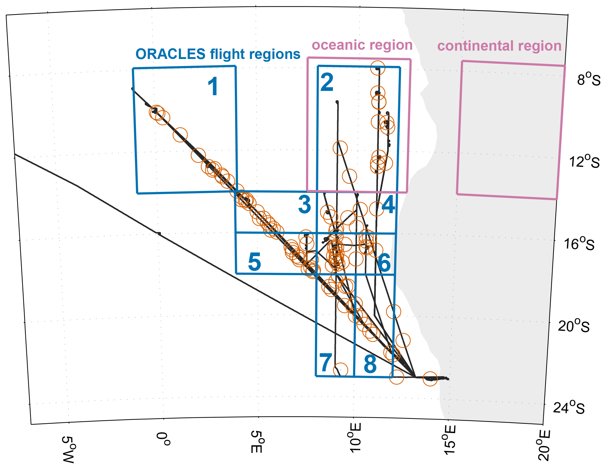
Figure 1Map showing the flight tracks of the 14 P-3 flights during ORACLES-2016 (black lines) and the areas of study in this work. Note that the SE-to-NW diagonal (passing through zones 1, 3, 5, 7, and 8) includes six routine flights overlaying one another. Reddish circles indicate locations of the 95 partial or full aircraft vertical profiles during all flights which will be discussed in more detail in Sect. 3.3. The blue boxes indicate the regional subsets (labeled zones 1–8) used in the spatially subdivided aircraft analysis in Sect. 3, and the lavender boxes show the oceanic and continental regions used for the reanalysis analysis in Sect. 3.4.
In the bulk of our analysis, we use carbon monoxide (CO) as a tracer of biomass burning emissions. CO is not aged or removed by cloud processes as the BB aerosols are, and thus it is a more reliable indicator of air mass origin than aerosol concentration. Modeled CO is also more robust than modeled outputs of individual aerosol species (e.g., Shinozuka et al., 2020) and thus allows for analysis of air mass origins and trajectories using these products. However, the results we show using observed CO are largely consistent with results using aircraft-measured aerosol extinction or scattering.
The NASA ORACLES (ObseRvations of Aerosols above CLouds and their intEractionS) campaign was a 5-year, multi-institutional project to study the effects of biomass burning aerosols and their interactions with the southeast Atlantic stratocumulus deck (Zuidema et al., 2016; Redemann et al., 2021). ORACLES had three field deployments during the African biomass burning season: out of Walvis Bay, Namibia, in September 2016, and out of São Tomé, São Tomé and Príncipe in August 2017 and October 2018. Each of these deployments used a NASA P-3 aircraft for tropospheric sampling (roughly 0–7 km), and the 2016 deployment had an additional high-flying ER-2 aircraft (above 20 km) for downward-looking remote sensing measurements. There are significant logistical and meteorological differences between each deployment; due to the different seasonal timing (by design of the ORACLES campaign) and the different deployment locations of 2016 versus 2017 and 2018, we analyze each deployment separately. In this work, we focus on data from the P-3 aircraft during the September 2016 deployment, with some discussion of the August 2017 and October 2018 observations to provide insight into the multi-year context. A more detailed discussion of the three ORACLES deployments may be found in Redemann et al. (2021). Figure 1 shows all P-3 flight paths and the locations of aircraft profiles for 2016 (i.e., the main focus of the present paper), as well as some key spatial delineations which we will use.
In Sect. 2, we introduce the instruments, data, and reanalysis and model products used. In Sect. 3.1, we present analysis of the atmospheric humidity as measured by three independent instruments aboard the P-3 aircraft, and in Sect. 3.2 we discuss how the water vapor relates to the presence of the biomass burning plume over the SEA in ORACLES-2016. We next compare the observations to reanalysis products and model outputs over the SEA (Sect. 3.3) and over the continental source region (Sect. 3.4). In Sect. 3.5 we briefly discuss the 2017 and 2018 observations and their key differences from the 2016 deployment. In Sect. 4, we synthesize the results before discussing potential causes of the observed patterns, their context within previous studies of the region, and their potential radiative implications.
In this work we use observational data from ORACLES in conjunction with large-scale atmospheric reanalysis and the outputs of specialized model configurations, as described below.
2.1 Aircraft instrumentation
The observational data considered here are from the ORACLES dataset. The full dataset is archived at https://doi.org/10.5067/Suborbital/ORACLES/P3/2016_V1 for the 2016 deployment, https://doi.org/10.5067/Suborbital/ORACLES/P3/2017_V1 for 2017, and https://doi.org/10.5067/Suborbital/ORACLES/P3/2018_V1 for 2018. All instruments used here were deployed on the P-3 aircraft during all three ORACLES deployments. Measurements at 1 Hz are used unless otherwise indicated. Individual flights were classified as either “routine flights”, which in 2016 extended along a diagonal flight path from 20∘ S, 10∘ E, to 10∘ S, 0∘ E, or “flights of opportunity”, which focused on specific science objectives and were generally nearer to the Namibian and Angolan coasts (Fig. 1). A more complete overview of the ORACLES operations and major results can be found in Redemann et al. (2021).
2.1.1 4STAR
The Spectrometer for Sky-Scanning, Sun-Tracking Atmospheric Research (4STAR; Dunagan et al., 2013) is an airborne hyperspectral (350–1700 nm) sun photometer which can make direct-beam (sun-tracking mode) measurements for retrieval of column aerosol optical depth (AOD; e.g., Shinozuka et al., 2013) and column trace gases (e.g., Segal-Rosenheimer et al., 2014) above the aircraft level. This work presents the column AOD and column water vapor (CWV) measured by 4STAR; additional ORACLES-2016 results using 4STAR measurements may be found in LeBlanc et al. (2020) for AOD and Pistone et al. (2019) for airborne retrievals of aerosol intensive properties using AERONET-like radiance inversions.
2.1.2 COMA
In all ORACLES deployments, volume mixing ratios of carbon monoxide (CO), carbon dioxide (CO2), and water vapor (q) were measured by a Los Gatos Research CO–CO2–H2O analyzer (known as COMA), modified for flight operations. It uses off-axis integrated cavity output spectroscopy (ICOS) technology to make stable cavity-enhanced absorption measurements of CO, CO2, and H2O in the infrared spectral region, technology that previously flew on other airborne research platforms with a precision of 0.5 ppbv over 10 s (Liu et al., 2017; Provencal et al., 2005). Water vapor measurements of less than 50 ppmv (∼ 0.03 g/kg) were removed due to instrument limitations, but this has minimal effect on the data considered here.
The CO measured during ORACLES is used in the present work as a tracer for air masses originating from combustion. While a major focus of ORACLES is the radiative effects of aerosols, CO will be conserved even under cloud processing which may affect the aerosol concentrations from biomass burning and thus provides valuable information on air mass origin (and simplifies the comparison to modeled parameters).
2.1.3 WISPER
Atmospheric water vapor was also measured as part of the Water Isotope System for Precipitation and Entrainment Research (WISPER), which reported H2O concentration and D H and 18O 16O isotope ratios. For ORACLES, WISPER was continued to use a pair of gas-phase isotopic analyzers based on the Picarro Incorporated L2120-i water vapor isotopic analyzer (Gupta et al., 2009). Coupled to the near-isokinetic solid diffuser aerosol inlet, the system reports total water (vapor plus condensate), which can be interpreted as vapor when out of cloud. Air was sampled from the inlet flow at 2.5 slpm via a 6 m long thermally insulated copper transfer line heated to 50 ∘C to minimize any wall effects and avoid possible condensation in the lines. The exterior portion of the SDI inlet was unheated. Two different Picarro L2120-i instruments were used during the 2016 campaign, one for the dates up to and including 4 September and another for later dates. The switch was associated with an instrument failure that led to poor data recovery on 3 of the 14 flights (Table 1). The instrument used in the first part of the campaign reports data at 5 Hz, while the instrument used later in the campaign reports at 0.5 Hz. Data from both instruments are aggregated onto a 1 Hz common time using simple binning and synchronized to the data system using cloud probes timing when entering/exiting clouds. Time synchronization has an uncertainty of about 1 s. Calibration of the system based on pre-campaign lab calibration using a LI-COR Model 610 dew point generator at a fixed temperature, with air diluted with ultra-zero grade dry air to span a low concentration range using quantitatively calibrated mass flow controllers. The water vapor measurements are valid to 10 ppmv (0.016 g/kg), and precision was typically reported as between 9–50 ppmv (0.01–0.08 g/kg), with greater values corresponding to a lower absolute water vapor amount.
2.1.4 P-3 aircraft data
The P-3 aircraft is equipped with instrumentation to make a number of standard onboard measurements of environmental data such as temperature, pressure, relative humidity, and wind speed. A full description of the onboard instrumentation may be found in Sect. 4.6 of the aircraft handbook at https://airbornescience.nasa.gov/sites/default/files/P-3B%20Experimenter%20Handbook%20548-HDBK-0001.pdf (last access: 21 June 2021). Following Vaisala (2013), the aircraft-based specific humidity (q) considered here was calculated from the reported dew point temperature (from an EdgeTech Model 137 aircraft dew point hygrometer) and static pressure (from a Rosemount MADT 2014 sensor) values:
where pmeas is the measured static pressure, mr is the ratio of the molecular weight of water vapor to air (), and pws is the simplified formula for water vapor saturation pressure over water given as
Here Tdp is the measured dew point temperature and the constants A, m, and Tn are 6.116441 hPa, 7.591386, and 240.7263 ∘C, respectively (Vaisala, 2013). The static pressure measurements have a precision of 0.5 hPa and an accuracy of ±2.5 hPa. For the dew point hygrometer, measurement precision was 0.1 ∘C and an accuracy of 0.2 ∘C nominally, with greater uncertainty below 0 ∘C and during profiles with large values.
2.2 Large-scale reanalyses and models
In conjunction with these observations, we select two large-scale reanalyses, which assimilate satellite observations and thus should be consistent with conditions observed by aircraft, and two free-running models, which, due to their unconstrained nature, may help to diagnose which processes are/are not in play. The reanalyses considered are the latest iteration of the ECMWF reanalysis, ERA5 (Copernicus Climate Change Service, 2017) and NASA's MERRA, Version 2 (MERRA-2; Gelaro et al., 2017). The former was chosen due to its exceptionally good agreement with the ORACLES observations (Sect. 3.3), and the latter was chosen as it incorporates aerosol observations, the lack of which is a shortcoming of the ERA product. We also briefly show results using the previous ERA-Interim (Dee et al., 2011) for continuity with previous work.
For the models, we consider two different specialized configurations of WRF developed in support of the ORACLES mission, termed WRF-CAM5 and WRF-Chem for consistency with previous studies (e.g., Shinozuka et al., 2020). The similarities and differences between each of these products is not the focus of the present paper, but the results of the differences between each product allows us to diagnose the influence of potential drivers in the real world.
2.2.1 ECMWF reanalyses
The European Centre for Medium-Range Weather Forecasts (ECMWF) has developed global atmospheric reanalysis products for several decades, with the ERA-Interim (Dee et al., 2011) serving as the primary reanalysis product through mid-2019, before being surpassed by the recently released ERA5 (Hersbach et al., 2019). ERA5 is considered at 0.25∘, hourly resolution, in the comparison with ORACLES flights (Sect. 3.3), and 0.25∘, 3-hourly resolution, in the continental analysis (Sects. 3.4 and 4.1). ERA5 does not report atmospheric chemistry or aerosols, nor does it directly incorporate aerosol effects, though satellite measurements of aerosol-influenced radiances are incorporated into the reanalysis. ERA-Interim was only available at a 3-hourly resolution. Due to the timing in the ERA5 dataset release, we explore results using both of these products in Sect. 3.3 and find ERA5 performs generally better compared to the observations. In the Supplement (Figs. S1 and S2) we provide selected comparisons between ERA5, ERA-Interim, and observations over the SEA.
2.2.2 MERRA-2
The Modern-Era Retrospective Analysis for Research and Applications, Version 2 (MERRA-2) is an atmospheric reanalysis produced by NASA's Global Modeling and Assimilation Office (GMAO) (Gelaro et al., 2017; Randles et al., 2017; Buchard et al., 2017). MERRA-2 assimilates observations of meteorological parameters from multiple satellite platforms, as well as aerosol optical depth from satellites (MODIS, AVHRR) and ground-based (AERONET) measurements, into a comprehensive atmospheric model, with assimilated aerosol fields explicitly entering the calculation of radiative heating rates within the model. MERRA-2 includes daily varying BB emissions from QFED (Darmenov and Silva, 2015), with a prescribed diurnal cycle which peaks in the mid-afternoon. MERRA-2 datasets are given on a nominal 50 km horizontal resolution (0.5∘ × 0.5∘) with 72 vertical layers from the surface to 0.01 hPa. An additional goal of the ORACLES campaign was to evaluate chemical transport models and reanalysis products such as MERRA-2, and to this end the complete set of MERRA-2 files has been sampled up to a 1 s resolution along every ORACLES flight (Collow et al., 2020). These products are available online at https://portal.nccs.nasa.gov/datashare/iesa/campaigns/ORACLES/. Over the larger continental and oceanic domain, MERRA-2, as with ERA5, is considered at a 3-hourly temporal resolution.
2.2.3 WRF-CAM5
The WRF-CAM5 configuration was run at a 36 km horizontal resolution over the month of September 2016, with 72 vertical layers (50 layers below 3 km) with a domain of 14∘ N to 41∘ S, 34∘ W to 51∘ E. It used CAM5 aerosol and physics, with MAM3 aerosols and CESM cloud microphysics and cumulus, with shallow cumulus turned off. Smoke emissions were from QFED, with no inversion and no plume rise. This model was initialized every 5 d, with 2 d of spin-up for each initialization (i.e., 3 d continuous runs at a time). Aerosol initial conditions were from the previous cycle, while the meteorology for each initialization was from NCEP-FNL-ANL, with chemistry and aerosols from CAMS reanalyses. We also note that here the ORACLES along-track WRF-CAM5 outputs are used at 10 s resolution. A more detailed description can be found in Shinozuka et al. (2020).
2.2.4 WRF-Chem
The WRF-Chem simulations were performed for the period of 15 August to 30 September 2016 at a 28 km resolution and 67 vertical levels covering a domain from 13.9∘ N to 35.6∘ S, 26.5∘ W to 42.5∘ E. Daily QFED biomass burning emissions were used following a diurnal cycle with a maximum at 14:00 local time (normal distribution), with additional EDGAR HTAP (Emissions Database for Global Atmospheric Research Hemispheric Transport of Air Pollution) anthropogenic and MEGAN (Model of Emissions of Gases and Aerosols from Nature) biogenic emissions. Radiation and aerosol–meteorology feedback were turned on, and a smoke plume rise process was enabled.
Initial and boundary conditions from ERA5 and CAMS reanalysis were used to account for the meteorology and chemistry and aerosols, respectively. Simulations were initialized every day at 00:00 Z and ran for 30 h. The first 6 h were discarded to account for the meteorology spin-up. We consider the period between 15–31 August (17 d) as spin-up for chemistry and aerosols. CAMS was used for boundary conditions during the whole simulation to account for possible intrusion of aerosols outside the domain (e.g., Saharan dust, smoke from Madagascar, sea salt). CAMS was used only for the 15 August initialization, and subsequent simulations were initialized by recycling the chemistry and aerosols from the previous run. In this manner, we can assume that all chemistry and aerosols used here are explicitly calculated by the model. In contrast, ERA5 was used for initialization and boundary conditions throughout the whole simulation (i.e., at daily reinitialization).
2.2.5 NOAA HYSPLIT trajectories
We ran NOAA's Hybrid Single-Particle Lagrangian Integrated Trajectory model (HYSPLIT; Stein et al., 2016) to trace air masses sampled by aircraft profiles towards their origins. Runs were computed offline using a standard HYSPLIT back-trajectory configuration. As ERA5 is not currently available as a HYSPLIT meteorological input, the meteorology used is from the National Centers for Environmental Prediction (NCEP) Global Data Assimilation System (GDAS) 0.5∘ model, provided directly by NOAA HYSPLIT (ftp://arlftp.arlhq.noaa.gov/pub/archives/gdas0p5, last access: August 2019), which is the highest resolution available for 2016. Trajectories are run using vertical motion determined alternately by the default “model motion” (kinematic trajectories using winds from the GDAS meteorology) and using isentropic pathways calculated from GDAS potential temperature fields (https://www.arl.noaa.gov/documents/workshop/NAQC2007/HTML_Docs/trajvert.html, last access: August 2019).
3.1 Measured humidity from different ORACLES instruments
Before presenting the analysis of the BB plume as it relates to the humidity, we first show the robustness of the water vapor measurements by comparing the three independent instruments available during ORACLES: COMA, WISPER, and the dew point hygrometer (aircraft) data from an onboard instrument (Table 1), as were described in Sect. 2.
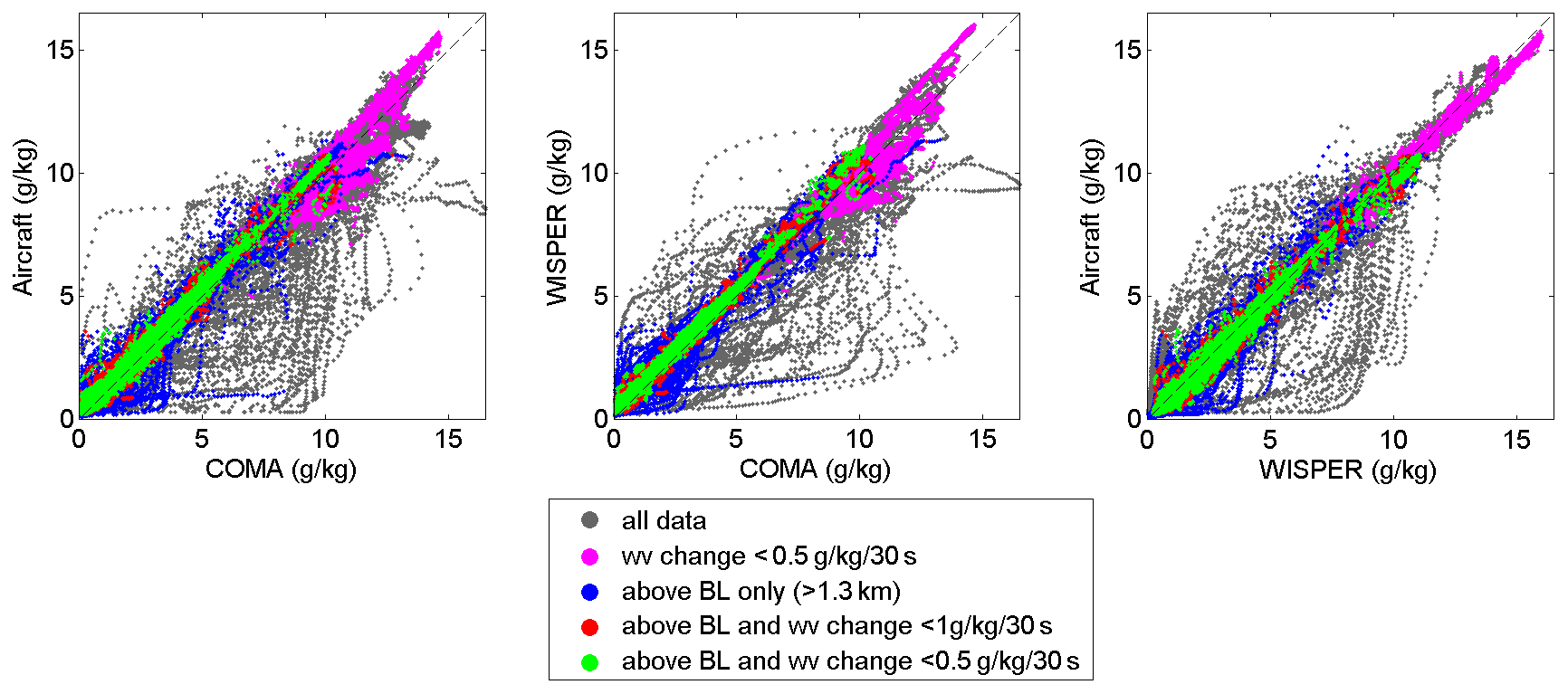
Figure 2Comparison of water vapor specific humidity q from the three instruments for ORACLES-2016, for all flight data and for subsets based on altitude or change in water vapor with altitude. This subsetting highlights that the majority of the disagreement between instruments (grey dots) is within the planetary boundary layer and/or during aircraft ascents/descents through rapidly changing conditions.
Figure 2 shows measurements from the three water vapor instruments for all 2016 flights at a 1 s resolution, for the full dataset and for specific subsets based on altitude (i.e., excluding layers which are clearly boundary layer altitudes) or water vapor gradient (i.e., to minimize the effect of varying instrument response times and inlet lengths). The correlations in all cases are robust and statistically significant (R2>0.97 for all data; Table 2), likely due in part to the large dynamic range and the volume of data collected. The colored subsetting highlights that the significant deviations from the 1 : 1 line (grey dots) occur either during high humidity conditions within the planetary boundary layer or during a rapid change in water vapor conditions, which can be explained in part as due to inlet differences and related issues of differing instrument response times. Deviations are expected during transitions from high q to low q or vice versa (e.g., from in-cloud to out-of-cloud conditions and to a lesser degree at the top of the plume layer) since each inlet system has differing heating to manage (or otherwise avoid) condensation artifacts. Additionally, the aircraft three-stage chilled mirror hygrometer specifically suffers from relatively poor temporal response during times of aircraft vertical motion or significant water gradients. Thus, aircraft moisture measurements are less reliable than during periods of straight, level flight or homogeneous conditions. Focusing specifically on the remainder of the data (largely in-plume conditions), we find that the instruments show quantitatively consistent water vapor measurements, with slopes of total least-squares fits between 0.98 and 1.01. These strong correlations between independent instruments on the same platform indicate that the observed water vapor signal is robust.
Table 1Data availability from each in situ instrument, as a percentage of all flight time (takeoff to landing), 30 August–27 September 2016, and as a fraction of only the in-plume level leg or vertical profile flight time (40 % of total flight time). A large portion of instrument downtime was during transit periods above the plume level.
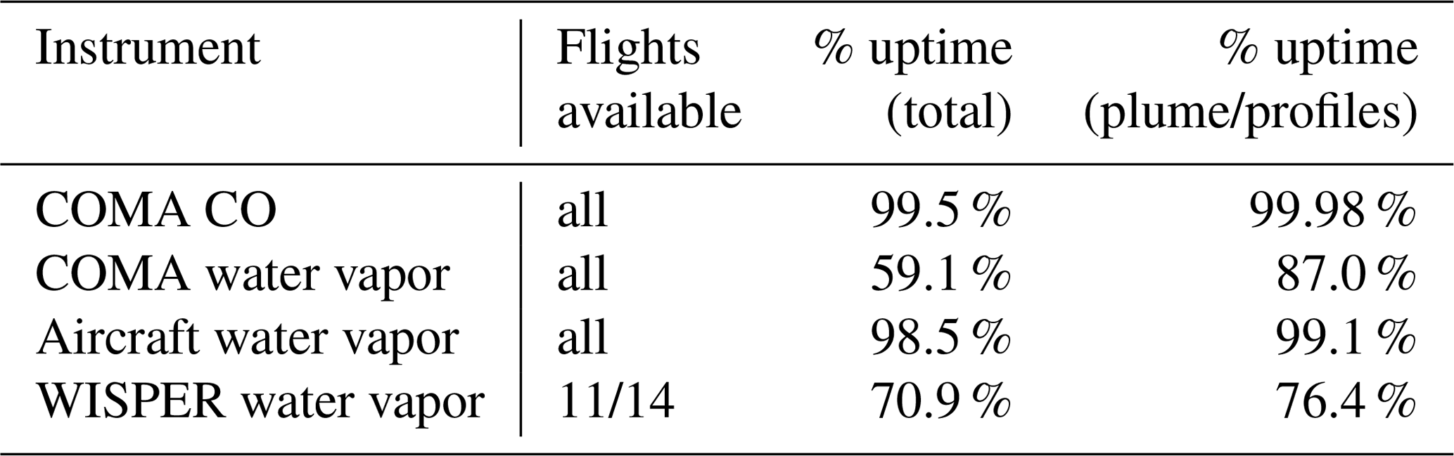
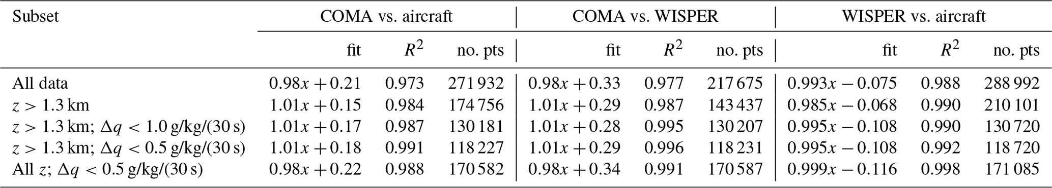
Table 2Correlations between measures of water vapor for ORACLES 2016, 1 s data resolution, for the subsets shown in Fig. 2. All correlations are significant at the p<0.001 level; the statistical significance and the slopes of the correlations are largely similar for each subset.
Having established that we have good confidence that the water vapor data are robustly measured by multiple instruments, in the following sections, we focus largely on COMA water vapor. This instrument measures q with greater precision than the aircraft probe, and more data are available from COMA than from WISPER for flight times either within the biomass burning plume or profiling the full atmosphere (Table 1), which are the sampling times on which we focus in this study. Additionally, while temporal corrections have been applied to synchronize the various instruments against one another, COMA CO and q are measured through the same inlet and thus are directly coincident. The majority of the missing COMA data were during above-plume transit legs (49.1 % of the missing data) and/or occurred under conditions of very low humidity outside of the biomass burning plume (62.7 % of the missing data) due to the 50 ppmv minimum instrument threshold of COMA. Regardless, the results are substantially similar using any of the water vapor content datasets.
3.2 Observed plume–water vapor correlations
3.2.1 ORACLES in-plume measurements
Examining the correlation between the biomass burning tracer CO and the water vapor content q within the plume layer (i.e., excluding boundary layer altitudes, here defined as below 2 km), we see a consistent pattern of elevated humidity with high CO. Figure 3 shows correlations between CO and q for each individual flight, for all altitudes above 2 km. Note that while an actual determination of boundary layer height is more complex (as described by Ryoo et al., 2021), here we choose a simple cut of 2 km as our goal is to focus on plume altitudes and exclude data with boundary layer influence. We find similar results for a variety of spatial, altitudinal, and temporal subsets above the planetary boundary layer; in other words, there does not appear to be a single altitudinal or latitudinal range which dominates this relationship for the dataset as a whole. We note that the results are similar for inlet-measured aerosol extinction and scattering coefficients (Fig. S3). The amount of water vapor seen here is consistent with the 5 g/kg moisture levels reported by Deaconu et al. (2019) for August and September (compared with 2.5 g/kg in June and July), and indeed during ORACLES we frequently see values of 6 g/kg or greater in the free troposphere.
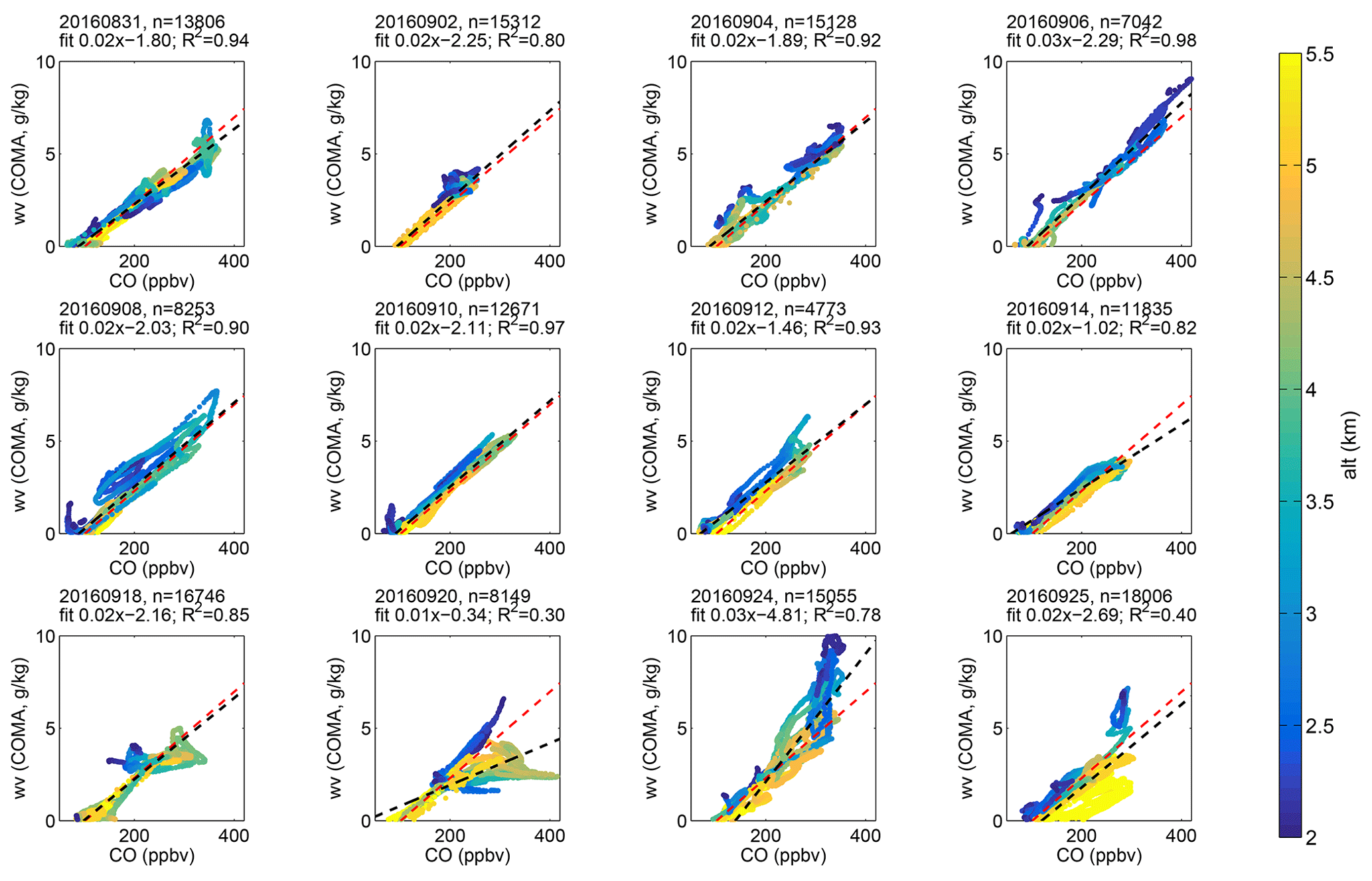
Figure 3ORACLES-2016 specific humidity versus CO, by flight. Here we show only altitudes substantially above the planetary boundary layer (> 2 km), so as to highlight the correlations at plume level. Dashed black lines show the total least-squares fit to each individual flight (z>2 km), and the red line shows the fit through all flights combined. All correlation coefficients are significant to two decimal points (p<0.01).
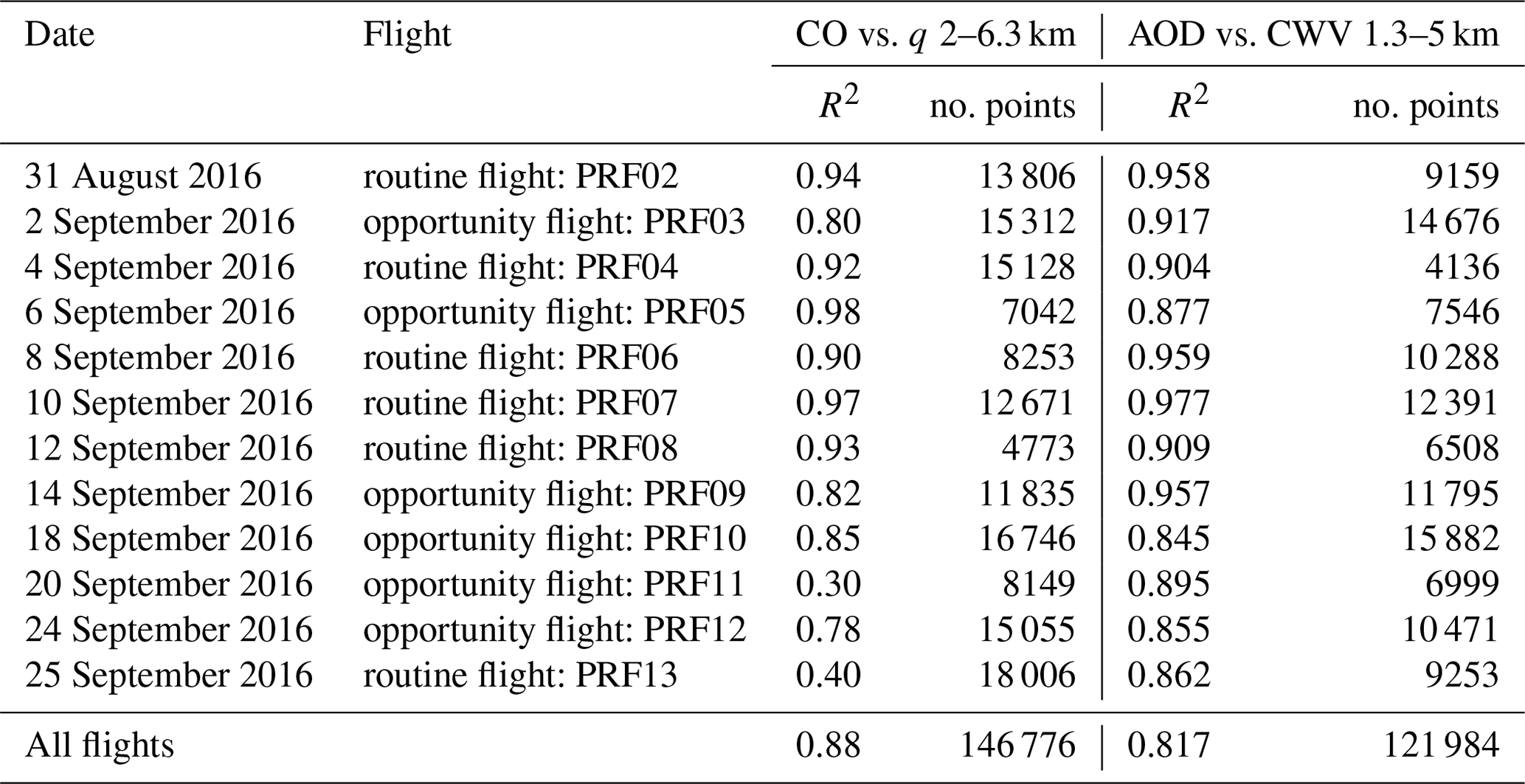
Table 3Correlations between free tropospheric CO and q (z>2 km) from in situ instruments as shown in Fig. 3 and correlations between AOD and CWV (z>1.3 km) from 4STAR as shown in Fig. 5, by flight for ORACLES 2016. All correlations are significant to p<0.001. Note that the different altitude limits are due to different methodologies. The terms “routine” and “opportunity” indicate whether the flights were along the northwest diagonal or near the coast (Sect. 2.1).
Each of the flight days in Fig. 3 shows a robust linear correlation, and some of the flights show especially linear correlations between CO and q, specifically the flights on 8, 10, 12, and 14 September 2016 (middle row). The first three of these flights were along the routine diagonal covering a fairly significant portion of the SEA extending northward to 10, 13.5, and 9.5∘ S, respectively. The flight on 14 September is classified as a radiation flight of opportunity, and while it did not follow the routine path, it still sampled somewhat diagonally from Walvis Bay (out to 16∘ S and a maximum westward extension of 7.5∘ E). While the correlations appear as generally stronger for routine flights, most of the flights of opportunity show strong correlations as well (R2>0.8; Table 3). The notable exceptions to this are the flights on 20 and 24 September which were both particularly close to the coast; when subdivided spatially over all flights, the relationship is more variable for the more southern coastal areas (Fig. 4). On 20 September, dust was also observed during a portion of the flight; this could indicate that the air mass sampled on these days had a different origin and different trajectory upon exiting the continent (i.e., directly easterly), compared with the typical conditions of the elevated biomass burning aerosol layer (i.e., a more northwesterly recirculation from an origin at AEJ-S latitudes). On 24 September, an unusually high boundary layer height was observed with westerlies below 3.5 km; this anomalous meteorological condition between 15–20∘ S may be responsible for the slightly weaker correlation that day. Returning to the routine flights, the flight on 25 September has a lower correlation than the others. On this day we see a shift in the CO–q slope with altitude, which is not seen during other flights; for smaller altitude subsets during this flight, the correlation is stronger. We also note that these flights are the last flights of the deployment and thus may be capturing an expected seasonal shift in conditions compared with the flights earlier in September.
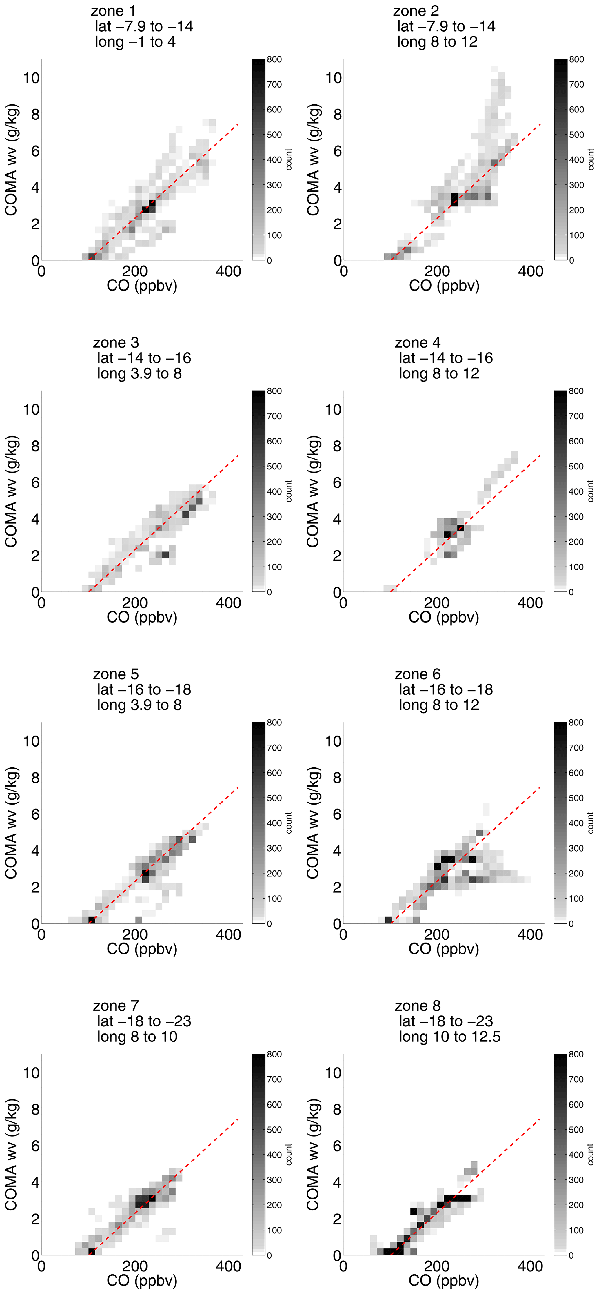
Figure 4 shows a frequency distribution of these same data subdivided spatially, highlighting how remarkably consistent the slope of this relationship is. Humid, smoky air exits the continent at roughly 10∘ S in the southern African easterly jet (AEJ-S), but we see that even at higher latitudes (lower rows), farther from the latitudes of the AEJ-S, the CO–q relationship is strongly linear and with much the same range in values down to ∼18∘ S. The main exception is the coastal Zone 6 (16–18∘ S, 8–12∘ E; Fig. 1), which is influenced by the observations from 20 September as discussed above. Overall, this suggests that the range of concentrations observed is present as a given air mass exits the continent and is not progressively diluted via mixing during transport.
3.2.2 Column ORACLES measurements
The 4STAR retrievals of AOD and column water vapor (CWV) are measured along the aircraft-to-sun light path and thus represent the full above-aircraft air mass, rather than the values at the aircraft altitude. While some impact of ambient humidity is to be expected due to hygroscopic swelling of aerosols (increasing AOD), it is nonetheless still instructive to examine these parameters as they compare to inlet-based instruments. A previous study of the ORACLES-2016 data showed incidentally that the relative (versus specific) humidity of the plume was quite low: approximately half of the in-plume inlet-based measurements were made at an ambient RH< 40 %, which is the typical threshold for “dry” aerosol (Pistone et al., 2019). Another 30 % of the observations were at an RH between 40 % and 60 %. For the data presented here, fewer than 2 % of the measurements above 2 km were measured at an RH > 80 % (typically used as the threshold for “wet” aerosol conditions, e.g., Magi and Hobbs, 2003). Another prior study of the ORACLES-2016 data (Shinozuka et al., 2020) also estimated that the effect of aerosol hygroscopic swelling on extinction was fairly minimal in the free troposphere, with an ambient RH dry ratio of less than 1.2 for 90 % of measurements, suggesting the same may be true for AOD.
Figure 5 shows the correlation between the 4STAR AOD at 500 nm and the CWV for 1 s data from all 2016 flights from above the boundary layer (here, >1.3 km) to the upper plume level (≤5 km). The 4STAR instrument provides a different geometric perspective from that of the inlet-based measurements described above yet shows similar results, providing additional evidence of the observed linearity between q and smoke concentration. The different altitude ranges compared with Fig. 3 are due to the different instrument requirements and capabilities; i.e., 4STAR observations from within the plume give only partial vertical profiles as 4STAR measures only the air mass above the aircraft at a given time. Thus measurements from entirely below the BB aerosol plume are valid and even preferred for 4STAR, whereas the inlet-based instruments are less useful at lower altitudes when there is a lack of plume loading. The largest range in AOD (and CWV) is seen on 24 September, near the coast, consistent with Figs. 3 and 4.
The 4STAR observations demonstrate that the plume–vapor relationship is consistent through the plume column and not solely at the instantaneous altitudes and locations as seen by the inlet-based instruments. We note this is also consistent with the results of Adebiyi et al. (2015), who showed that upper-level (∼700 hPa, roughly 3.2 km) humidity from radiosondes corresponded to conditions of high AOD from satellites, albeit farther offshore at St Helena. The fact that we see a strong linear correlation between markers of the biomass burning plume and atmospheric water vapor from multiple instruments and over multiple flights is a strong indication of the robustness of this relationship over this region during the ORACLES-2016 time period.
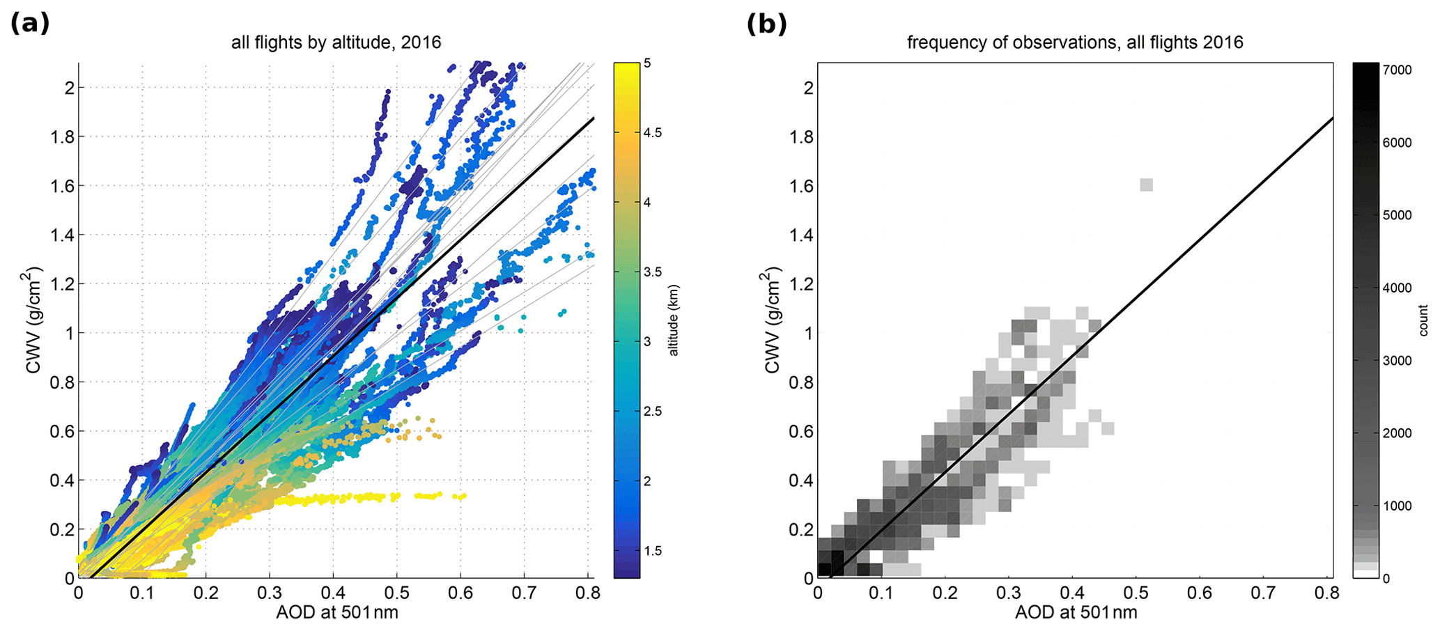
Figure 54STAR AOD at 500 nm versus column water vapor (CWV) for altitudes above the boundary layer to within the BB plume (1.3 to 5 km) (a) by altitude for all flights and (b) as a frequency heat map over all flights. Thin grey lines show the total least-squares fits through individual flights, while the thicker black line shows the fit through all data. The correlation coefficients are fairly high for individual flights (Table 3) and only slightly lower for all flights combined (R2=0.82).
3.3 Do reanalyses/models capture the relationship seen in the observations?
Having established the robust CO–q relationship over the southeast Atlantic Ocean as seen in these observations during ORACLES-2016, we next seek to explore the larger mechanisms by which this relationship has developed. The source region for ORACLES BB observations includes widespread seasonal grassland savannah fires over central and southern Africa (e.g., van der Werf et al., 2010; Redemann et al., 2021) and sees little variability in either fuel source or combustion efficiency (e.g., Vakkari et al., 2018). We wish to take a broader perspective which incorporates these continental regions, which is not possible using solely the over-ocean ORACLES aircraft data. Thus, we turn to reanalyses and model simulations.
Figure 6 shows the ORACLES flight data from aircraft profiles aggregated and subset to times and altitudes corresponding to the ERA5, ERA-Interim, and MERRA-2 reanalyses and the WRF-CAM5 and WRF-Chem models, with different reanalysis altitude ranges distinguished by color and shape. We note that this is a subset of the data shown in Fig. 3, but the CO–q relationship shown here is consistent with that of the full dataset. For each of the altitude ranges – boundary layer (square), boundary-layer-influenced (triangle), or plume level (circle) – there is good agreement between ERA5 and the aircraft observations (Fig. 6a) from the surface through the plume level. An exception is at altitudes at the top of the boundary layer ( ∼ 570 m; squares), where ERA5 often underestimates water vapor, perhaps due to difficulties in determining boundary layer height over the ocean surface. Despite this, the humidity at surface level agrees well with the observations, and, more importantly in the context of this study, the existence, magnitude, and location of elevated water vapor for plume altitudes are also well represented in ERA5. It is reassuring that this newest ECMWF product agrees so well with the aircraft observations (R2=0.79 for z>2 km), and this gives us confidence that the ERA5 meteorology may be consistent with real-world meteorology over the continental source region as well. Figure 6b and c show the comparisons between aircraft-observed q and ERA-Interim and MERRA-2 reanalysis q, respectively. Both of these correlations are rather weaker than that for the ERA5 reanalysis (R2=0.53 and R2=0.40 for ERA-Interim and MERRA-2, respectively) but still largely capture the presence of an elevated water vapor signal in the altitudes above the boundary layer. However, both these products also often report this high-humidity air as being at a lower altitude than what was observed by the aircraft observations (an example is shown in Fig. S2).

Figure 6ORACLES water vapor measurements compared with reanalyses and models subset to the locations of aircraft profiles and altitudes of ERA5 outputs. Observations are averaged within ±50 m of the reanalysis levels; MERRA-2 reanalysis is averaged over the time of the aircraft profile and interpolated to ERA5 altitudes for ease of comparison. Free tropospheric altitudes are shown by circles; smaller squares are the boundary layer, and triangles are intermediate altitudes. Here we see that (a) the ERA5 water vapor and the observed water vapor subset to ERA5 altitudes show good agreement within the plume layer and for the lower boundary layer (R2=0.79 for z>2 km); agreement is poorer for (b) ERA-Interim (R2=0.53), (c) MERRA-2 (R2=0.40), and (d) WRF-CAM5 (R2=0.48), although a linear CO–q relationship is still seen. (e) WRF-Chem initialized from ERA5 shows better agreement (R2=0.79).
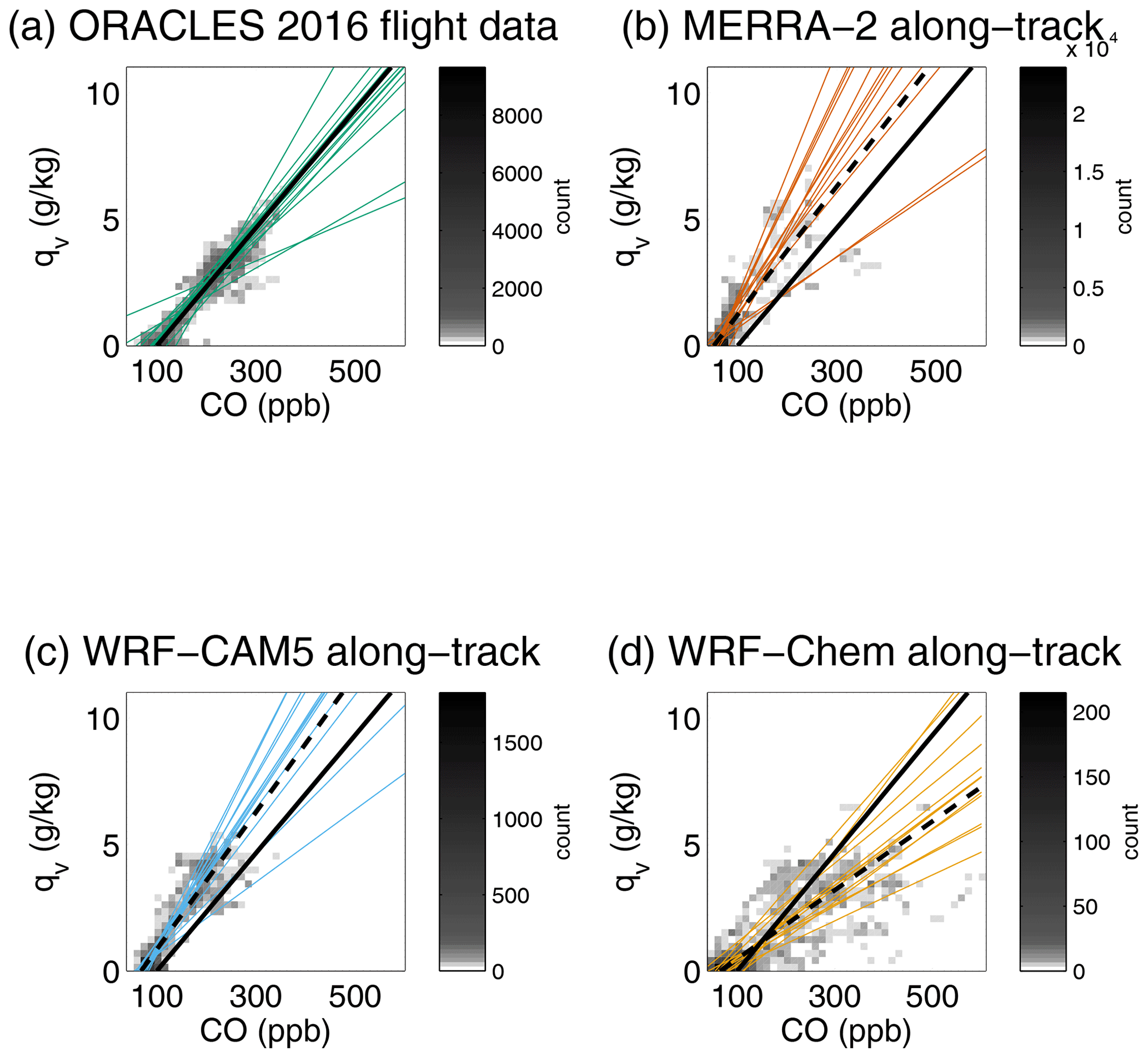
Figure 7CO vs. q from (a) aircraft observations (R2=0.78), (b) MERRA-2 reanalysis (R2=0.56), (c) WRF-CAM5 (R2=0.71), and (d) WRF-Chem (R2=0.49) for all flights, for altitudes z>2 km. Individual colored lines show the total least-squares fits for individual flights, and the black lines show the averages of all observed flights (solid) compared to each model (dashed).
Finally, Fig. 6d and e show the two configurations of WRF described in Sect. 2.2.3 and 2.2.4. WRF-Chem q shows a strong correlation with the observed q, in line with that of ERA5 (R2=0.79 for both products for all altitudes >2 km), which is not surprising due to WRF-Chem's daily initialization with ERA5 reanalysis meteorology. The WRF-CAM5 water vapor is more weakly correlated with the observed water vapor (R2=0.48, more in line with the results from MERRA-2 and ERA-Interim). This difference is likely due in part to the different meteorological fields used (NCEP versus ERA5), and also to WRF-CAM5's less frequent initializations (5 d versus 1 d), allowing it to drift farther from the “actual” meteorology and chemistry conditions between initializations. Given these results alone, one might be discouraged by the possibility of using MERRA-2 or either WRF configuration in this analysis, but this is not the full story. Although the water vapor co-location is poor, we find that the relationship between CO and q does hold over the flight path (Fig. 7). Here, interestingly, the results are flipped: MERRA-2 and WRF-CAM5 show comparatively better correlations between CO and q (R2=0.56 and R2=0.71, respectively, compared with R2=0.78 in the observations), while WRF-Chem now shows more variability in CO–q conditions and thus a poorer correlation between the two (R2=0.49). The fact that the CO–q correlation is fairly high for MERRA-2 and WRF-CAM5 even while the observed–modeled q correlation is low essentially indicates that while these two products are not placing a given air mass exactly where and when it was observed by the aircraft, the consistent relationship between the plume and water vapor is maintained, simply in an alternate location. We must also consider the differences in model emissions and meteorological configurations to potentially explain this. MERRA-2 and the WRF models all use QFED emissions, albeit with different implementation in each. Because WRF-CAM5 has the best correlation between CO and q and the longest independent run length, it seems plausible that the periodic reinitialization of each model's meteorology independent of its emissions weakens the correlation between the two. This would be because the reinitialization will “correct” the meteorology (water vapor) towards the reanalysis at the same time that the chemistry (CO) is adjusted independently and to a different degree than the meteorology. This would explain why the 3 d runs (5 d minus 2 d spin-up) of WRF-CAM5 show a stronger correlation than WRF-Chem (with daily reinitialization) or the MERRA-2 reanalysis. We also note that MERRA-2 and WRF-CAM5 report lower CO for higher water vapor (i.e., the slope between the two variables is steeper than in the observations), whereas the opposite is true for WRF-Chem. Overall, this pattern suggests that the CO–q relationship is sustained through dynamics affecting both properties equally – i.e., not through diabatic processes such as cloud formation which could decrease the water vapor – and moreover that this holds within the considered models. Given this context, we conclude that, while not perfect, the different strengths (and limitations) of each of these models may be useful in understanding the mechanisms involved in the real world.
Figure 8 shows vertical profiles of water vapor from COMA subdivided spatially by latitude and longitude grids according to the boxes shown in Fig. 1 (the same divisions used in Fig. 4), with routine flight paths in the left column and coastal flights on the right. Each subplot shows profiles of the nearest co-located ERA5 reanalysis points, for comparison. This spatial division by aircraft profile highlights both the consistency in the vertical structure of the plume observed by aircraft and shown by ERA5 and the differences in this vertical structure in different regions of the SEA. In terms of the spatial differences, Zone 2 (top right) has consistently the highest measured water vapor (4–11 g/kg) and CO, possibly due to its proximity to the location of the AEJ-S (∼10 ∘S). Also, along the routine diagonal (i.e., farther from the coast), we more frequently see a dry/clean gap between the humid plume and the more humid boundary layer, plus a greater plume strength compared with the near-coast regions at the same latitude (see also Fig. 4). In contrast, the more coastal flights often see either more humid, higher-CO air masses at lower altitudes or constant CO and q at all altitudes (Fig. 4). Finally, we note that Fig. 8 shows again how consistently well the ERA5 reanalysis performs when compared to the aircraft observations, even in the case of a varying profile type. There is a good deal of variability in this structure in different latitude/longitude ranges (e.g., high- and low-altitude plumes with substantial vertical variation or a fairly consistent magnitude with altitude), but these differences are consistent between both ERA5 and the observations.
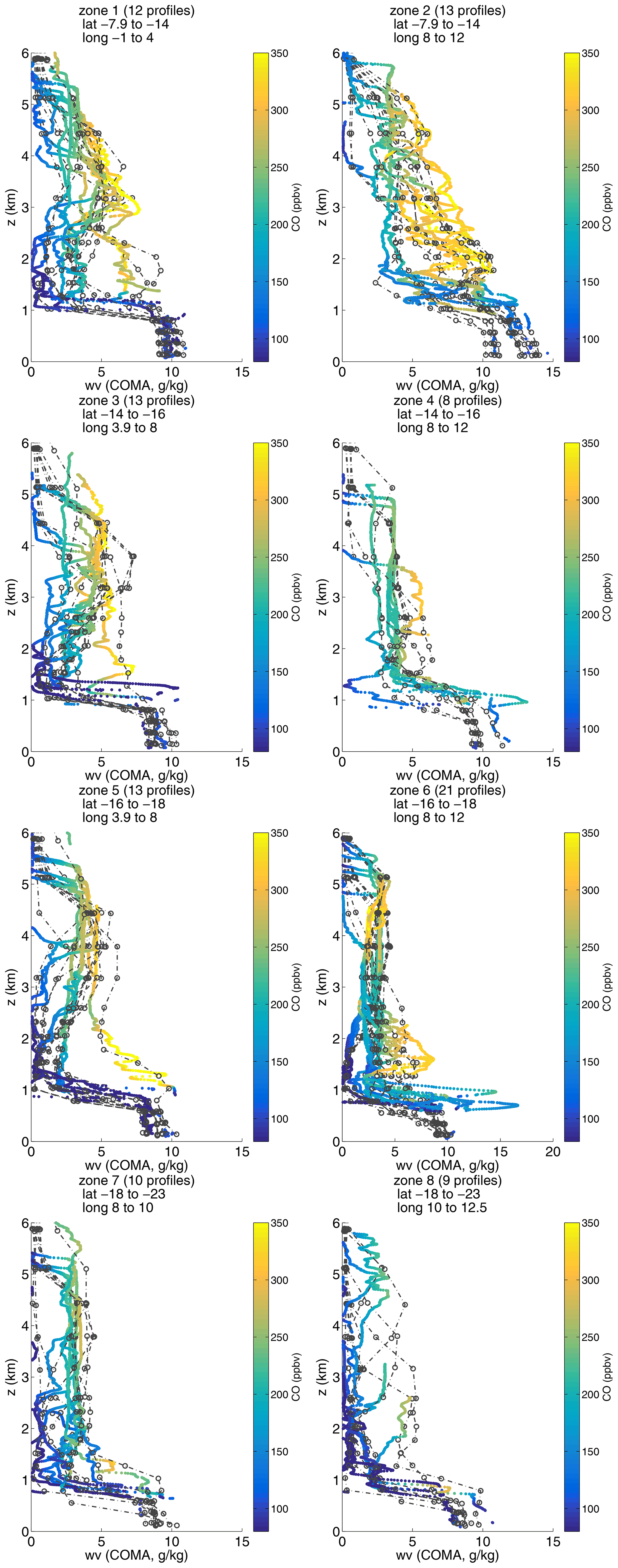
Figure 8Profiles of specific water vapor measured by COMA in ORACLES-2016 (solid lines), subdivided by spatial location. Colors indicate the CO concentration from COMA. Dash-dotted lines show spatiotemporally co-located ERA5 reanalysis profiles for each aircraft profile, which captures the variability in vertical structure reasonably well.
3.4 The larger-scale perspective shows continental origins of the linear relationship
Our results thus far are consistent with previous satellite- and reanalysis-based work which described both the same pattern of elevated water vapor coinciding with biomass burning aerosols over different parts of the SEA (e.g., Adebiyi et al., 2015; Deaconu et al., 2019) and the importance of the southern African easterly jet (AEJ-S) in transporting continental air masses over the southeast Atlantic Ocean (e.g., Adebiyi and Zuidema, 2016). Having shown that several models and reanalyses are able, to some degree, to capture the presence of an upper-level water vapor signal during ORACLES-2016, in this section we focus on the reanalyses to gain more insight into the origins of this pattern over the biomass burning source region. Specifically, we may reasonably expect that due to the excellent agreement between the ERA5 reanalysis and the observations in the ORACLES SEA sampling region, ERA5 may give an accurate picture of meteorological context for the air mass origin over the continent and its evolution during its westward transport. MERRA-2, while not as directly translatable to aircraft measurements, may yet allow us to complete the picture by showing how q relates to CO concentration.
Figure 9a shows a Hovmöller time series of ERA5 atmospheric water vapor with longitude at 600 hPa (∼4.4 km; identified by Adebiyi and Zuidema, 2016, as the altitude of max AEJ-S strength), averaged over 7.75–14∘ S. These latitudes are chosen to encompass the usual range of the AEJ-S while overlapping with the upper extent of the ORACLES flight data (zones 1 and 2 in Fig. 1). These q contours are overlaid with average horizontal wind vectors at the same altitude. A few features are obvious from this reanalysis: first, multi-day episodes of high water vapor conditions are seen to originate over the continent and are advected westward when zonal wind speeds are high. That is, an elevated water vapor signal is frequently present at up to 5 km over the continent and these humid air masses are transported in the easterly jet only under conditions of high zonal wind speeds. Second, we note that there is a notable diurnal cycle in q over the continent, likely driven by the diurnal cycle in the continental boundary layer development. The timing of the diurnal maximum q varies substantially with altitude (as will be discussed shortly). While Fig. 9 shows the 600 hPa pressure level, the results are largely the same for pressure altitudes 700–500 hPa (i.e., the range of the AEJ-S; Adebiyi and Zuidema, 2016) and for latitude subsets within this range. For more southern latitudes, the reanalysis shows much weaker zonal winds, less water vapor at higher altitudes, and no direct connection between continental and over-ocean conditions at the same latitude; the direct east–west transport is not observed. While the AEJ-S ranges from 5–15∘ S, between ∼5 and 8∘ S there is likely a combination of dry and moist convection present, whereas dry convection is likely to dominate south of 10∘ S. Either type of convection will result in elevated q at the AEJ-S altitudes. This pattern of transport, i.e., recirculation of smoky, humid air from the north to the south, is consistent with the BB source region being at more equatorial latitudes even for the more southern ORACLES observations, as was also shown by Adebiyi and Zuidema (2016). The broader meteorological features were discussed in more detail in Redemann et al. (2021) and Ryoo et al. (2021).
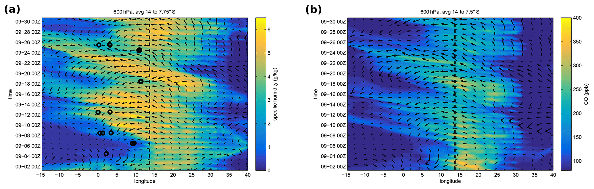
Figure 9Hovmöller plot showing the development and transport of air masses from continental Africa over the SEA, with colors showing (a) water vapor from ERA-5 and (b) carbon monoxide from MERRA-2, at 600 hPa (∼ 4.4 km), based on 3-hourly time steps. The location of the African shoreline in this region is indicated by the dashed black line, and data are averaged between 7.75 and 14∘ S (note the domain is slightly larger for MERRA-2 due to the model resolution). Black circles show the locations and times of ORACLES aircraft profiles within this region. In the east (right-hand side) of each plot, the diurnal convection cycle is evident, showing increased water vapor (CO) at this altitude during the daytime; in the west (left-hand side), episodes of water vapor (CO) are seen as these continental air masses are advected by the AEJ-S. Wind vectors do not scale between the two panels, although the patterns are seen to be largely similar between the two reanalyses.
A similar pattern is seen in CO reported by MERRA-2 (Fig. 9b): periodic events of westward CO transport are co-located with water vapor transport events, driven by the zonal winds. Both the zonal winds and water vapor are generally similar between the MERRA-2 and ERA5 reanalysis. The water vapor and CO are qualitatively similar in the WRF models as well, although we observe a distinct discontinuity in the time series of these models which corresponds to the (daily for WRF-Chem or every 3 d for WRF-CAM5; Fig. S4) reinitialization. This lends credence to the idea that model reinitialization may be responsible for the weaker correlations in these products (WRF-Chem in particular; Fig. 7), as q and CO are adjusted to differing degrees during this process. The fact that the correlations persist between reinitializations but then are lost again suggests that any removal/mixing processes over the SEA Ocean affect CO and q equally; i.e., the air is not subject to significant diabatic processes or cloud formation during transport, which could lower q without affecting CO.
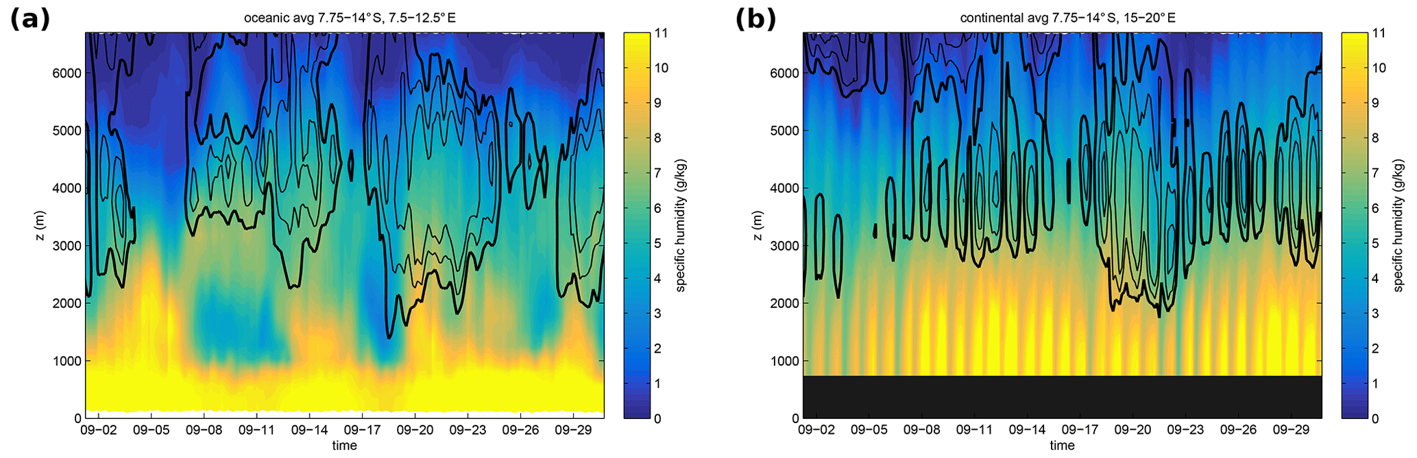
Figure 10Oceanic (a) and continental (b) specific humidity (shaded) overlaid with zonal wind speed (black contours) from the ERA5 reanalysis. The thick black lines indicate the threshold of the AEJ-S (6 m/s) with thin black lines showing 8 and 10 m/s easterly velocities.
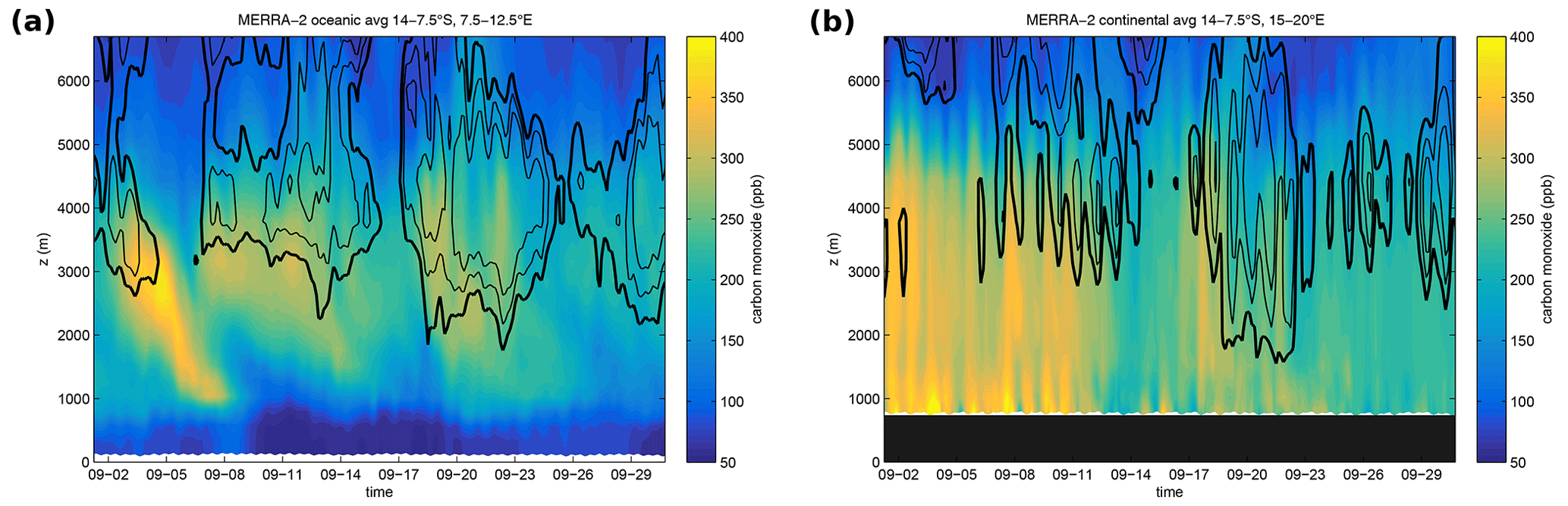
Figure 11Oceanic (a) and continental (b) CO (shaded) overlaid with zonal wind speed (black contours) from the MERRA-2 reanalysis. The thick black lines indicate the threshold of the AEJ-S (6 m/s) with thin lines showing 8 and 10 m/s easterly velocities.
Figure 10 shows a time series of the vertical profiles of ERA5 humidity, over the same latitude range as that in Fig. 9, averaged over two distinct longitude ranges (lavender boxes in Fig. 1): the eastern continental source region (Fig. 10b, 15 to 20∘ E) and the western ORACLES region (Fig. 10a, 7.5 to 12.5∘ E). Selected zonal wind speed values are overlaid as black contours (the thickest line shows the 6 m/s easterly zonal velocity threshold for the AEJ-S (as in Adebiyi and Zuidema, 2016), with thinner lines showing 8 and 10 m/s). With the exception of early in the month, when a baroclinic disturbance was present to the south, the AEJ-S is seen to be almost always present and centered around 4 km (∼650 hPa) in both these domains, though the jet varies in magnitude both on a diurnal cycle and throughout the month. Although there are multi-day humidity (and AEJ-S) episodes, over the continental source region there is strong diurnal variation in both zonal wind speed and water vapor content which is dampened once the jet exits the continent.
Figure 11 shows the MERRA-2 winds and CO over the same two regions. The pattern is similar: MERRA-2 also shows the frequent presence of the zonal jet, with a strong diurnal cycle in wind speed over land, and the CO values again indicate boundary layer influence reaching to above 5 km, propagating upward in time. While the presence of the AEJ-S over the SEA corresponds to significant carbon monoxide, we also see how this high-CO air mass may disperse out into the broader region (e.g., the episode starting around 4 September at 3 km over the ocean region is transported down to 1 km by 6 September in the absence of the strong zonal winds). The direct comparison between MERRA-2 profiles and aircraft observations suggested a potentially too-strong subsidence, resulting in a lower-altitude q maximum (Figs. 6, S2); indeed, Das et al. (2017) previously documented a subsidence in MERRA-2 which was greater than that inferred from satellite observations. For this particular instance there was a sustained downward motion at 700 hPa in both ERA5 and MERRA-2 between 4–6 September, which may be responsible for this episode seen in both reanalyses (Figs. 10a, 11a). Regardless, even in a case of too-strong subsidence in MERRA-2, this issue itself will not affect the relationship between CO and q once it is over the SEA but rather just its location. It is clear from the two reanalyses that continentally influenced air over the SEA remains for a sustained period of time and is transported both horizontally and vertically throughout the region while retaining high q and high CO amounts.
Further insight can be gained by examining the diurnal cycle directly at individual pressure levels. Figure 12 shows time series of key meteorological parameters: zonal winds, water vapor, pressure vertical velocity, and potential temperature (u, q, ω, and θ, respectively) from ERA5 and the same parameters plus CO from MERRA-2, at constant pressure levels of 550 and 650 hPa (approximately 5.1 and 3.7 km; just above and below the AEJ-S maximum). The bottom panels of Fig. 12 show the diurnal cycles of each day normalized to scale between a unitless 0 and 1 and then averaged over all days in September 2016. While this does not provide any information on the magnitude (this is captured in the panels above), it does illustrate the relative timing of the minima and maxima of each variable through the diurnal cycle, and it provides a qualitative idea of the consistency of this diurnal cycle throughout the month (i.e., when the maximum in an average curve approaches 1 as u650 hPa at 15:00 Z, this is an indication that wind speed consistently peaks at that time each day; in contrast, the flatter curve of CO650 hPa shows that the diurnal cycle either does not vary throughout the day or peaks at different times of day throughout the month; from the panel above for CO, we can see in this case the former applies). Taken together with the upper panels, this visualization allows us to examine the strength of the diurnal variations compared with multi-day events, how each of these parameters at a given altitude is offset from the others at the same height, and thus the range of air mass conditions which exit the continent in the AEJ-S.
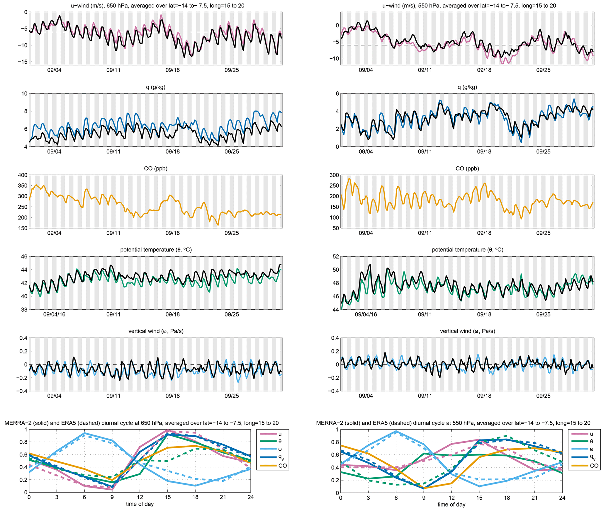
Figure 12Time series of (top to bottom) zonal winds (u; m/s), specific humidity (q; g/kg), CO (ppb), potential temperature (θ; ∘C), and vertical velocity (ω; Pa/s), at 650 hPa (left) and 550 hPa (right) for MERRA-2 (colored lines) and ERA5 (black lines) reanalyses. Distinct diurnal cycles are seen for all variables except CO at 650 hPa, where variability is dominated by multi-day changes rather than a strong diurnal cycle. The 650 and 550 hPa panels for a given parameter are on the same scale so as to highlight differences in diurnal cycle magnitudes with altitude, though shifted to capture the full range at each level. Shading indicates night (18:00–06:00 UTC). The horizontal dashed line in the u panel shows the 6 m/s AEJ-S wind speed threshold (Adebiyi and Zuidema, 2016), and the horizontal dashed line in the ω panel shows the 0 Pa/s threshold which separates rising (−ω) from sinking (+ω) vertical motion. Note that easterly u winds are given by negative values. The bottom panel shows the composite diurnal cycle for each variable from MERRA-2 (solid) and ERA5 (dashed) overlaid on one another (colors the same as above), normalized to a diurnal minimum of 0 and maximum of 1 and then averaged over all September days.
In the previous figures, we saw a daily upward propagation in the continental water vapor (Fig. 10b) and a similar feature in CO (Fig. 11b), likely due to diurnal heating causing daytime boundary layer growth over the land. This convection allows the surface air to mix upward and reach strikingly high altitudes (∼5 km) during the day, but the vertical motion is influenced by upper-level subsidence at night. A more detailed discussion of boundary layer height is given in Ryoo et al. (2021); as their calculated boundary layer height differs from the value reported in ERA5, we do not go into detail here regarding a quantitative analysis. However, the altitudes up to 6 km are clearly seen to be surface-influenced as seen in the parameters we consider, even if they may not be well-mixed with the surface. In Fig. 12, we note that this pattern propagates upward with a delay: while daily maximum humidity at 750 hPa (∼2.6 km) was generally around 09:00–12:00 Z, the maximum at 650 hPa varies between 12:00–18:00 Z, and at 550 hPa it is still later, between 15:00–21:00 Z. Again we note there is both daily variation and multi-day episodes, which both vary with altitude. Specifically, the diurnal variability in q is strong at both 650 and 550 hPa, whereas for CO, there is a distinctly stronger diurnal cycle at 550 hPa; the reverse is true for u, which has larger daily variation at 650 hPa. The diurnal cycle also varies throughout the month, with a somewhat weaker diurnal cycle in both CO and q when the zonal winds are strongest (e.g., 19–21 September).
We note that while the water vapor over the African continent shows a strong diurnal cycle due to solar heating, the fire strength also has a diurnal cycle following the anthropogenic burning patterns (Roberts et al., 2009). While these timings vary based on location, they generally peak in the late afternoon and are almost entirely extinguished by nightfall (Roberts et al., 2009), which is fairly similar to the timing of the solar-forced daily evaporation and convection over the continent. As mentioned earlier, in this region, the fire characteristics themselves are fairly consistent over this period (fuel type, combustion efficiency, and burn condition). These patterns are incorporated into the modeled emissions schema. While the multi-day CO variation does not closely track with that in q, the timing of the peaks for an individual day is largely consistent between CO and q at both levels (minima at 09:00 Z, maxima between 15:00–18:00 Z; Fig. 12 bottom row). CO at the lower altitude varies substantially over the course of several days (∼100 ppbv), and the 550 hPa CO consistently varies by 50–100 ppb within a 24 h cycle, with the maximum CO between 18:00 –00:00 Z, suggesting frequent influence from dry, clean air above. This suggests that the 550 hPa level is influenced by upper-level subsidence and mixing on a daily basis, whereas the values at 650 hPa are influenced more by surface influence and transport in the AEJ-S.
Another piece of the puzzle is the dynamics. Daytime vertical motion over the continent is dominated by solar heating and subsequent convection, as is seen in the substantial daytime increase in potential temperature and the upward propagation of both humid and high-CO air. Overnight, convection is reduced and (when the AEJ-S is active) the zonal wind generally increases, advecting this air to the west. During times of weak-to-no AEJ-S (e.g., first week of September 2016), the decreasing q and CO overnight at 550 hPa is accompanied by frequent strong subsidence and increasing θ (due to the subsidence from above in the absence of solar heating), which suggests increased stratification which would inhibit vertical mixing. The vertical velocities in Fig. 12 show more frequent subsidence (+ω) at 550 hPa versus 650 hPa, and ω at both levels has a maximum (downward velocity) in the early morning (06:00 Z) and a minimum (upward motion) in the late afternoon (15:00–18:00 Z), which is consistent with convection caused by diurnal heating. In contrast, during times of strong jet activity (e.g., 18–22 September), the jet still largely strengthens overnight and q and CO decrease, but potential temperature also decreases. Since CO and q still generally decrease during this time, this may indicate that increased shear mixing is happening when the jet is strong, which decreases the CO and q values by mixing the more humid and smoky continentally influenced air with dry, clean upper-level air. When AEJ-S conditions are weak and when the potential temperature is relatively high, large-scale subsidence dominates and stabilizes the atmosphere without much mixing between air masses at this interface.
This distinction between high-jet and low-jet conditions is corroborated by Fig. 13. This figure shows the CO–q correlations from the MERRA-2 reanalysis along one longitude line over (right) the continental source region and (left) the oceanic ORACLES sampling region for the surface-influenced altitudes and for the free troposphere, respectively. For all data within the full boundary layer over land (top right), the relationship is not as coherent as that observed during ORACLES, and at individual altitude levels below 550 hPa the linear relationship is nonexistent (Fig. S5); the low-CO, low-q data are almost entirely driven by the higher altitudes (>600 hPa). In Fig. 13, there is also a frequent condition of (relatively) high q (∼12 g/kg) and low CO (<300 ppb) which does not correspond to any particular altitude level. In other words, this humid air with a wide range of CO values is often present at altitudes subjected to AEJ-S conditions, rather than being confined closer to the surface (Fig. S5), yet it was not observed over ocean during ORACLES. At the same time, the linear relationship is seen over the SEA Ocean for these same latitudes (Fig. 13, top left); this is puzzling, since based on our previous analysis (e.g., Fig. 9), we expect the eastern continental region to be the direct source for the western oceanic region. When we consider only the conditions of strong easterly transport (Fig. 13, bottom), the situation becomes clearer: now, the CO–q relationship over the continent is much closer to the linear relationship observed over the ORACLES region and is largely similar to the ocean data as a whole. Similar patterns are seen in both WRF configurations (Fig. S6), with a stronger high-q, low-CO feature, likely due to differences in biomass burning implementation between each model.
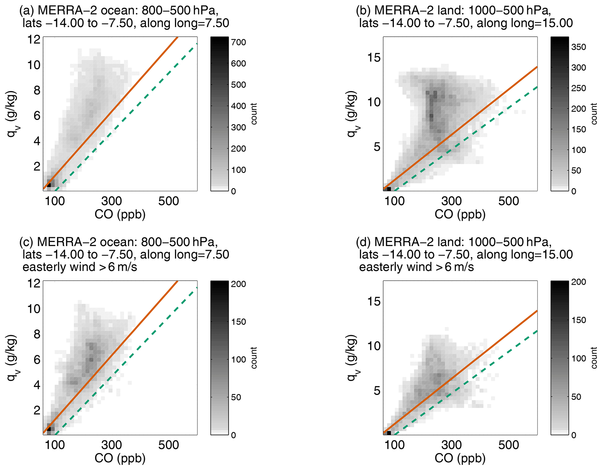
Figure 13MERRA-2 CO and water vapor over land and over ocean, for (a, b) all observations along 15 and 7.5∘ E and (c, d) only observations for which easterly wind speed was >6 m/s. For orientation with previous results, the dashed green line is the fit through all ORACLES-2016 free-troposphere flight data and the solid red line shows the MERRA-2 fit coincident with the aircraft observations (both as in Fig. 7). A vertically resolved version of this plot is shown in Fig. S5. The results are largely similar for WRF-CAM5 and WRF-Chem (Fig. S6).
It is notable that if we consider the CO–q relationship of Fig. 13b for only one jet level (e.g., the jet maximum of 600 hPa), there is no obvious linear CO–q relationship at all over land (Fig. S5). Only starting at the 550 hPa level does a linear relationship begin to emerge, primarily driven by low-q, low-CO conditions. These higher altitudes are at times alternately influenced by both clean, dry upper-troposphere air and humid, smoky surface-influenced air (Fig. 12). According to MERRA-2, these values decrease in altitude (as expected) from 5–12 g/kg in q and 200–500 ppb in CO at 700 hPa to 0–5 g/kg in q and 60–300 ppb in CO at 500 hPa. While the maximum q continues to decrease above 500 hPa, dropping to 1 g/kg at 400 hPa, even at this high altitude the CO does not fall below 60 ppb. While this may be due to the emissions schema used rather than physical reasons, this is nonetheless consistent with the minimum CO observed by aircraft during ORACLES, suggesting the modeled background CO is accurate.
It thus seems plausible that the mixing between surface and upper-troposphere air is occurring over the continent, resulting in a vertical gradient from the surface up through the altitudes of the AEJ-S. Due to the frequent upward convection along with diurnal variations in potential temperature and in zonal winds, air masses with a specific range of co-associated conditions are selected by the AEJ-S, thus effectively converting these vertical gradients into horizontal gradients over the SEA. Thus the mixing occurs over the continent and the resulting mixed air masses are transported over the SEA having this range of properties, which is what results in the same linear pattern being present over the broader SEA region. The linear relationship observed during ORACLES is the result of air which left the continent at multiple different levels within the AEJ-S range and which was subjected to the AEJ-S conditions.
3.5 Results from the 2017 and 2018 deployments
As the ORACLES-2016 data represent only about one-third of the data collected during ORACLES, we wish to briefly discuss the context of the latter two ORACLES deployments. As discussed in Sect. 1, the ORACLES-2017 and ORACLES-2018 deployments differed from ORACLES-2016 in several key ways. Each deployment occurred, by design, during a different month (September, August, and October in 2016, 2017, and 2018, respectively) and thus saw different climatology. The spatial sampling was also significantly different in the 2 later years (i.e., more northerly; Fig. 14) due to the moving of the deployment base to São Tomé. Even between the 2 latter years, the 2018 flights were generally closer to the continent, whereas the 2017 flights included a series of flights to, around, and from Ascension Island at 14.4∘ W (this runway was not available in 2018). Sampling the more equatorial air masses in 2017 and 2018 means these flights sampled more humid air and a deeper boundary layer (Fig. 15) even after accounting for the expected seasonal climatological changes. As the biomass burning season peaks in September and shifts geographically through the season, the plume itself, as well as the prevailing meteorology, would have been different even if the flights had occurred from the same base in all 3 years (Redemann et al., 2021). Aside from this, the ORACLES analysis found that there was significant interannual variability from year to year such that some years saw a peak in BB in September and some saw the peak in August. A more detailed discussion of the broader meteorological and aerosol contexts may be found in Ryoo et al. (2021) and Redemann et al. (2021).
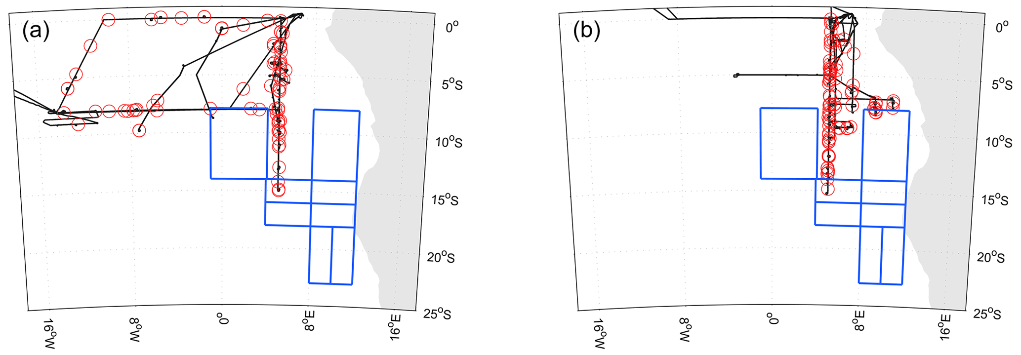
Figure 14Map showing the flight tracks of (a) the 12 science flights + 2 transit flights by the P-3 in ORACLES-2017 and (b) the 13 science flights + 2 transit flights by the P-3 in ORACLES-2018. The blue boxes give the regional subsets used in Fig. 1 and Sect. 3.3, which highlight the difference in spatial sampling between 2017–2018 and 2016. While few flights in these years fell within these boxes, quite a few (including the routine flight path) were within the 7.75 to 14∘ S latitude range shown in Figs. 9 and 10. Note that while the routine flights in 2016 followed a SE-to-NW diagonal, the routine flight path in the 2 later years was N–S along 5∘ E.

Figure 15ORACLES-2017 (left) and ORACLES-2018 (right) water vapor vs. CO, for selected flights, for the subset of latitudes overlapping with the 2016 sampling region (south of 7.5∘ S; colored) and for the remainder of data at all latitudes above 2 km (grey). The thick blue lines show the fits through all 2017 (2018) flights, and the purple lines indicate the fits through the portions of the 2017 (2018) flights which are south of 7.5∘ S and east of 0∘ E. The thick dashed red lines show the fits through all 2016 flights as in Fig. 3. The variation in this relationship from year to year is evident.
Figure 15 shows the CO–q relationship above 2 km for a subset of 2017 and 2018 flights. A few key differences are evident between Figs. 3 and 15. The most prominent difference is that while the two values are still largely correlated, the near-universal linearity between CO and water vapor observed in 2016 is largely absent in 2017 and 2018 as a whole (grey + colored points). However, when considering only observations within the same spatial range as that of 2016 (south of 7.75∘ S and east of 0∘ E; colored points), the correlations are stronger. We note the total least-squares fits through the full dataset (dashed blue lines) versus 2016 overlap (dashed lavender lines) are not significantly different for each year, likely due to the dynamic range in CO and q values in both subsets. The more equatorial observations (grey points) are frequently high-humidity–low-CO observations largely at lower altitudes, particularly in October 2018, indicating boundary layer influence may extend higher than 2 km in this year (Ryoo et al., 2021). The differences between the three deployments are likely due to the anticyclonic atmospheric circulation at AEJ-S latitudes towards the south. In other words, seasonal variation aside, the 2016 deployment simply sampled more air masses which were influenced primarily by the BB plume, rather than other more northern origins seen in the latter 2 years. August 2017 more frequently saw higher-CO air masses with relatively lower water vapor compared with the other two deployments. August climatologically sees more northern continental convection (compared to in September and October, when the convection migrates south with the end of winter) and also has a much weaker AEJ-S; the AEJ-S was especially weak in 2017 (Ryoo et al., 2021), which may also be a factor in the weaker correlations during this deployment. Of the 3 years, the correlation coefficients between the two parameters are highest in 2016.
The weaker correlations and more humid conditions are thus likely caused by a combination of upward mixing of the oceanic boundary layer in the latter years, the seasonal change in biomass burning sources, and the more equatorial meteorology sampled in 2017 and 2018. A more complete analysis of the factors which influence the patterns in these years will be the subject of a future work.
Thus far, we have established that (1) there is a robust linear correlation between water vapor and BB plume strength as measured from several distinct aircraft instruments; (2) this elevated water vapor feature appears, with varying fidelity, in both meteorological reanalyses and free-running climate models; (3) there is frequent deep boundary layer daytime convection over the continent which causes humid, smoky air to be lofted to the altitude of the AEJ-S, which transports it westward; and (4) the linear CO–q relationship is seen over the continent but only concurrently with a strong AEJ-S condition. We now attempt to synthesize these findings to paint a coherent picture of the evolution of this condition between its source on the African continent and its observation with the ORACLES aircraft using two examples from the flights. Then, we will briefly explore whether the high water vapor content may be due to some characteristic of the biomass burning itself or due to some other cause.
4.1 Trajectories from emission to observation
Figure 16 shows the example of an ORACLES aircraft profile (ramp) from 10 September 2016 at approximately 10:00 (09:58:50–10:10:33 UTC) centered at 15.6∘ S, 5.6∘ E (south of the AEJ-S range; Zone 3 in Fig. 1). We choose this profile as it showed multiple plume layers of varying strength: a main plume layer starts around 3.5 km, strengthens to 4 km, and continues above the aircraft range (∼ 4.2 km in this case), with a secondary peak in CO and q around 2.4 km and a layer of low CO and low q between the two (∼ 2.8 to 3.2 km). Below the second plume layer, there is a gap of much cleaner air around 1.5 km, just above the boundary layer. The second reason we choose this profile is that since the ERA5 reanalysis captures these features fairly well at this time and place, including the smaller secondary q below 3 km. (We note that MERRA-2 shows this feature as well (dashed purple line), although the main plume layer is displaced too low in altitude compared with the observations).
Figure 16b shows HYSPLIT back trajectories from three locations within this profile: 4 km (the maximum plume), 3.1 km (the local minimum), and 2.4 km (the smaller local maximum). Back trajectories are run for 6 d both for isentropic (constant θ) pathways and using the GDAS so-called model motion (kinematic trajectories using vertical winds from the GDAS meteorology). For this case, at the two higher altitudes, these trajectories (while over the SEA Ocean) are remarkably similar to one another in terms of latitude and longitude, which allows us to speculate on the implications of each configuration. For a given initial altitude, the two trajectories diverge in trajectory altitude, with the kinematic trajectories showing consistent subsidence (when looking forward in time) and the isentropic trajectories being fairly constant in altitude (at least after they depart the continent), but the two trajectories are very similar in terms of horizontal location, at least after exiting the continent (beyond that point, the trajectories become more uncertain due to convection over land).
Finally, Fig. 16c–e show these trajectories overlaid on the ERA5 reanalysis fields of water vapor (blue shading) and potential temperatures (θ, grey contours show isentropes at 3 K intervals), following the location of the isentropic trajectories. Here we can clearly see that the differences between the two trajectories are most pronounced in the vertical. We note that the isentropic trajectories as given by HYSPLIT (lines with circles) correspond to isentropic contours from ERA5 (grey curves) at all altitudes until the trajectory reaches (or rather, exits) the continent: on 8 September for the 4 km trajectory, and on 7 September for the 3.1 km trajectory. The 2.4 km trajectory is over the ocean during the entire trajectory and thus follows the isentropes for this entire period. Once trajectories are determined to be over the continent, they exhibit more variability in terms of altitude, as would be expected due to the strong convection in this region. This also likely indicates the trajectory analysis is less reliable beyond this point, but the trajectories are nonetheless consistent with air masses originating from a diurnally varying deep continental boundary layer around 5–10∘ S.
The kinematic (nonisentropic) trajectories, in contrast, are seen to cross many θ curves during this time, but this is not necessarily inconsistent with the ERA5 reanalysis: in terms of the water vapor, these back trajectories calculated using GDAS winds still remain within the humid layer for several days, until the trajectories are over the continent (4 km and 3.1 km on 8 and 7 September) or diverge from the isentropic trajectory (2.4 km on 8 September). We note that the 2.4 km trajectories diverged within 2 d of the analysis and the kinematic trajectory exits the top of this humid layer shortly thereafter; when the ERA5 reanalysis is considered along the remainder of the 2.4 km kinematic trajectory (i.e., at the HYSPLIT-indicated latitudes and longitudes), this trajectory too remains within the top of the water vapor plume until 3 September.
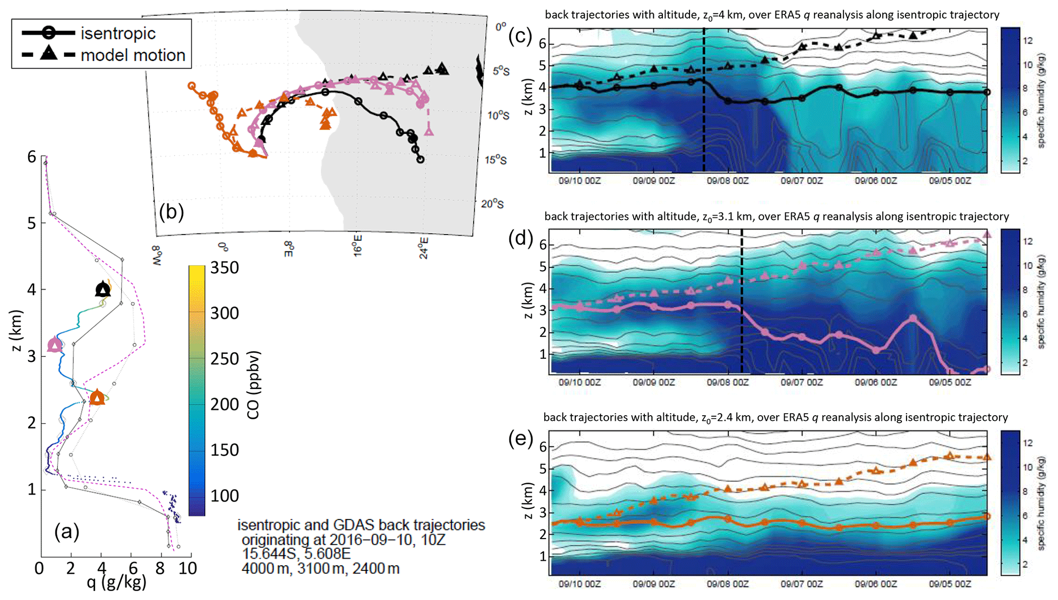
Figure 16(a) An ORACLES aircraft profile from 10 September 2016 at approximately 10:00 Z. Colors show the aircraft-measured CO corresponding to the measured water vapor, while the solid black, dotted black, and dashed purple lines show the ERA5, ERA-Interim, and MERRA-2 profiles at the same time and place. The map (b) shows HYSPLIT back trajectories originating at three altitudes (bold shapes in a) within this profile, and the right-hand panels show the ERA5 reanalysis q profiles (blue shading) at the location and time of the isentropic paths, starting at (c) 4 km, (d) 3.1 km, and (e) 2.4 km, overlaid with the ERA5 potential temperatures (θ, grey contours), and both the isentropic (solid line with circles) and kinematic (dashed line with triangles) HYSPLIT trajectories, for each altitude. Dashed vertical lines delineate when the 4 and 3.1 km isentropic trajectories pass over the continent.
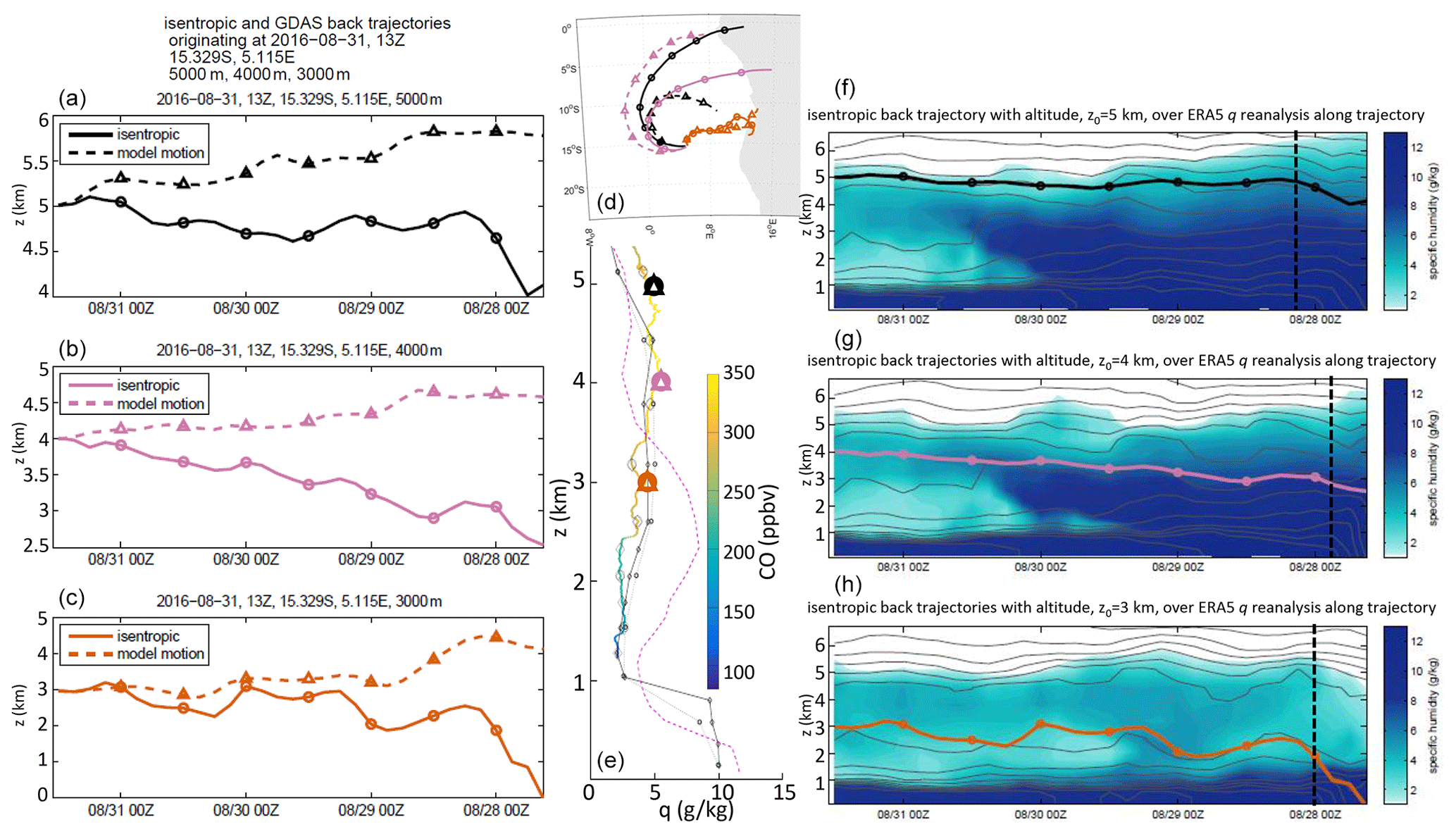
Figure 17As in Fig. 16, for three trajectories initialized from a profile from 31 August 2016 13:00 Z which showed more uniform q and CO with altitude than the profile on 10 September. Back trajectories are initialized at (a, f) 5 km, (b, g) 4 km, and (c, h) 3 km altitudes. As the isentropic and kinematic trajectories significantly diverge from one another in latitude and longitude, the trajectories in (f)–(h) show ERA5 values along the isentropic trajectories only. The altitudes of both back trajectories in time are shown in (a)–(c).
Taken together and considering the analytical caveats of each, these different perspectives on one sampling instance suggest that the air mass transport leading up to the aircraft observations may be somewhere in between the results of the two types of trajectory. We remember that a too-strong subsidence is an issue in models over this region; Das et al. (2017) showed that vertical velocities in several different models were frequently too large compared with CALIOP satellite observations, especially once air masses exit the continent. This is consistent with what we see here regarding very strong subsidence in the GDAS vertical motion, and suggests that the isentropic trajectories may be closer to the observed conditions. Yet the fact that the kinematic trajectories continue to follow the humid layer even with this strong subsidence indicates it is possible that these model trajectories are in the famous model category of “wrong, but useful”. Or rather, while the air masses sampled during ORACLES largely follow isentropic pathways, there is some influence from clean, dry free tropospheric air especially over the continent. Indeed, this would be consistent with what we see in Figs. 12 and 13: the linear relationship between CO and water vapor over the continent is largely driven by higher-altitude air which is only periodically influenced by continental sources; without these influences, the conditions of low CO and low q would not be as prevalent in the air which is advected over the SEA.
The MERRA-2 trajectories may be less instructive as a direct comparison with HYSPLIT as the initial conditions do not match; however, they may provide some insight as to the evolution of the linear CO–q relationship. When considering along-path MERRA-2 CO and q for the strongly subsiding model motion HYSPLIT trajectories (not pictured), we do see a linear relationship similar to that in Fig. 6, which would be consistent with a similar correlation having developed over land due to mixing from above (assuming that these trajectories have unrealistically strong subsidence over ocean).
As a final example, we consider the case shown in Fig. 17, for back trajectories initialized at the aircraft profile sampled just before 13:00 Z (12:35:21 to 12:50:14) on 31 August 2016, centered on 15.3∘ S, 5.1∘ E, in the same general area (Zone 3) as in Fig. 16. In contrast to the previous figure which was a very layered profile, this profile was fairly uniform in both q and CO with altitude; this is corroborated by ERA5 but again placed too low by MERRA-2. Here, when we run the HYSPLIT back trajectories using model motion and isentropic motion initialized at three altitudes (3, 4, and 5 km), we find that the two configurations diverge much more rapidly. Again we find that the model motion trajectories (from GDAS meteorology) show very strong subsidence while the isentropic trajectories actually show the opposite: rising motion going forward in time. Spatially, the two trajectories diverge in latitude and longitude much earlier than they did in Fig. 16, though both methods end up in largely the same location for the 4 and 5 km trajectories (Fig. 17d). Looking at the ERA5 reanalysis along these trajectories, we find that the isentropic trajectories agree fairly well with the presence of the elevated water vapor plume and some altitudes with fairly constant θ, which may indicate these trajectories are less reliable, causing the discrepancy. This highlights the limitations of this type of analysis.
4.2 Sources of continental plume water vapor
We now briefly discuss the initial source of this continental water vapor. There are several potential explanations for the correlation between water vapor and the SEA BB plume, including direct emission of water vapor as a product of combustion, water vapor co-emission due to fuel properties, enhanced surface evaporation or evapotranspiration from the burning regions, or simple meteorological coincidence between plume air and already-humidified ambient air. As both smoke and water vapor have their source in the continental boundary layer, it may purely be a coincidence of this source and further mixing with dry and clean free tropospheric air, but we briefly explore the other possibilities.
Regarding the first point, some amount of water vapor is co-emitted with other gases and aerosols during combustion. Parmar et al. (2008) measured the ratio of enhanced water vapor to carbon dioxide and emissions () for different vegetation types: for savannah grasses this ratio is ∼ 1.2–1.6 and for some trees it reaches up to ∼ 3. For the sake of argument, even for a relatively high ratio of 3 (which should be an overestimate of the amount of water we should expect from burning of savannah grass), this means that a 2 g/kg enhancement in water vapor would be accompanied by an enhancement of ∼ 800–1000 ppm of ΔCO+ΔCO2.
For all three ORACLES deployments, the vast majority of CO2 concentrations were measured as between 400 and 460 ppm and there were no measurements above 500 ppm. Based on these ratios and the CO2 and water vapor concentrations observed during ORACLES, burning biomass could only have increased atmospheric water vapor by a tiny fraction of what was observed. Unless the estimates either of the ratio of water vapor emitted per carbon dioxide and carbon monoxide or of the typical ΔCO+ΔCO2 plume enhancement are too low by orders of magnitude, it is not plausible that the linear CO–q relationship seen in ORACLES-2016 or the general moistness of the smoke plume is due to the co-emission of water vapor during biomass burning. The fact that the elevated water vapor (∼ 2–4 g/kg) observed during ORACLES is not associated with significantly elevated CO2 over the same region (on the order of 2000 ppmv) suggests that the water vapor at least is not a direct product of combustion.
Another possibility is that the moisture of the fuel itself could be evaporated during combustion; however, Potter (2005) suggested that for woody fuels, the fuel moisture would constitute no more than a third of the water vapor emitted by combustion, which would not account for the magnitude of the signal we observe. It is still plausible that some amount of the enhanced atmospheric water vapor near the fire sites could simply be a result of moist fuels releasing water vapor under the higher fire temperatures; alternately, the observed q could result entirely from surface evaporation/evapotranspiration independent of the fire conditions. Clements et al. (2006) also measured higher sensible and latent heat fluxes and increased turbulent mixing associated with the smoke plumes from small grass fires and concluded that vapor emissions from such fires would have measurable impacts on local atmospheric dynamics, which may also be in play here. However, regarding these last points, we find that models consistently reproduce some level of elevated q without including either a source of water vapor co-emitted from biomass burning or enhanced evaporation due to the higher surface temperatures in fire conditions, which suggests that these factors are not primary.
Thus, it seems likely that we can rule out direct co-emission of water vapor as the primary cause of the humid plume, and a simple meteorological coincidence seems to be the most likely explanation behind the observed correlations.
In the aircraft observations collected during the ORACLES field campaign over the southeast Atlantic Ocean, we find a robust correlation between plume strength, as indicated by both inlet-based CO concentration and column AOD, and water vapor concentration. The correlations are highly robust and linear in the September 2016 data and somewhat weaker in the more equatorial observations from August 2017 and October 2018. These year-to-year differences could be due to a variety of factors, including the difference in season, deployment location, and sampling patterns over the SEA (e.g., routine diagonal versus routine north–south leg).
The ERA5 reanalysis is particularly accurate in placing its high humidity as coincident with the higher humidity measured by ORACLES flights. All the other reanalyses/models showed a similar pattern of elevated humidity above boundary-layer altitudes but with varying degrees of agreement between modeled water vapor content and q from the aircraft observations. Considering the products which report CO, the CO–water vapor relationship shows an opposite pattern to that in q: the product which best corresponds to observed q (WRF-Chem) shows the least consistent correlation between CO and q. In contrast, both WRF-CAM5 and MERRA-2 show somewhat better correlation between CO and q but poorer correlation between modeled and observed q. This suggests that the CO–q relationship overall is better represented in a free-running model (versus one which is frequently reinitialized) likely due to the differing effects of this reinitialization on water vapor versus chemistry. However, such a free-running model results in a greater mismatch in the location of a given humid, smoky air mass compared with the observations (in latitude/longitude and in altitude).
On the regional scale, the ERA5 reanalysis shows humid air reaching high altitudes (700–500 hPa; 3–6 km) over the continent, albeit with a lag time from the surface. This is corroborated by other products. The analysis from MERRA-2 also indicates that the CO and q are in phase with one another at the plume level, despite day-to-day variability in the actual magnitudes of each. Large-scale analysis thus suggests the air masses sampled over the ocean in ORACLES left the continent with the same relationship between water vapor and carbon monoxide as that observed by aircraft. This linear relationship develops over the continent due to diurnal upward mixing within the deep continental boundary layer (max height ∼ 5–6 km) and this boundary layer top air mixes with the drier, cleaner free tropospheric air above to produce fairly consistent q and CO vertical gradients (decreasing with altitude) which vary in time. Due to a combination of conditions including differential advection at different levels; daytime convection; nighttime subsidence; timing of anthropogenic fires; and resulting mixing between the smoky, moist continental boundary layer and the dry and fairly clean upper-troposphere air above (∼6 km), the vertically aligned gradients are effectively stretched horizontally and into layer-like structures over the ocean. For conditions of strong zonal wind, the smoky, humid air is advected over the SEA following largely isentropic trajectories, where it persists, circulates, and in this case was sampled by ORACLES.
Water vapor, particularly when co-located with absorbing aerosols, will have significant impacts on both atmospheric radiative transfer (shortwave heating and longwave cooling) and cloud macrophysics and dynamics. An analysis which builds upon our results here – and other components of the ORACLES dataset – to quantify the radiative impacts of this water vapor on the atmosphere over the broader SEA may thus help to clarify or corroborate previous studies of these effects. Future work will also examine the year-to-year variation in this relationship and the contributions of the BB plume and the humid layer to atmospheric radiative heating and aerosol–cloud interactions within this stratocumulus deck.
The data used in this paper are publicly available at https://doi.org/10.5067/Suborbital/ORACLES/P3/2016_V1 (ORACLES Science Team, 2017) for the 2016 data and at https://doi.org/10.5067/Suborbital/ORACLES/P3/2017_V1 (ORACLES Science Team, 2019a) and https://doi.org/10.5067/Suborbital/ORACLES/P3/2018_V1 (ORACLES Science Team, 2019b) for the 2017 and 2018 data, respectively. The codes used in processing 4STAR data may be found at https://doi.org/10.5281/zenodo.1492912 (4STAR Team et al., 2018). ECMWF reanalyses are available at the Copernicus Climate Data Store (https://cds.climate.copernicus.eu/; Copernicus Climate Change Service, 2017). HYSPLIT is available through the NOAA Air Resources Laboratory (https://www.ready.noaa.gov/HYSPLIT.php; Stein et al., 2016), and the compatible GDAS half-degree meteorological data are found in the gridded meteorological data archives (https://www.ready.noaa.gov/archives.php; Rolph et al., 2017).
The supplement related to this article is available online at: https://doi.org/10.5194/acp-21-9643-2021-supplement.
KP designed the research, performed the analysis, and wrote the paper with substantial input and feedback from PZ, RW, and MD. LP, JMR, and RU contributed to the interpretation of the meteorological features and context. AMdS, PES, and GF contributed to the interpretation of the reanalysis and model results. AMdS provided the ORACLES-specific MERRA-2 reanalysis. PES provided the WRF-CAM5 model outputs. GF and GC provided the WRF-Chem model outputs. CF, SL, JR, MSR, and KP collected and processed the 4STAR data. JP collected and JP and YS processed the COMA data. DN collected and processed the WISPER data. ES collected and RB processed the onboard aircraft data. YS was the ORACLES data manager and compiled the observations. JR, RW, and PZ were the ORACLES principal investigators. All authors were provided with intermediate and final drafts of the manuscript for input and feedback.
The authors declare that they have no conflict of interest.
Publisher's note: Copernicus Publications remains neutral with regard to jurisdictional claims in published maps and institutional affiliations.
This article is part of the special issue “New observations and related modelling studies of the aerosol–cloud–climate system in the Southeast Atlantic and southern Africa regions (ACP/AMT inter-journal SI)”. It is not associated with a conference.
ORACLES is a NASA Earth Venture Suborbital-2 investigation managed through the Earth System Science Pathfinder Office. We thank the ORACLES deployment support teams; the ORACLES science team; and the governments and people of Walvis Bay and Swakopmund, Namibia, and São Tomé, São Tomé and Príncipe, for a successful and productive mission.
This research has been supported by the National Aeronautics and Space Administration through the Earth Venture Suborbital-2 (EVS-2) program (grant no. NNH13ZDA001N-EVS2). The WISPER data were collected with support from the NSF Atmospheric Chemistry and Climate and Large-scale Dynamics programs (grant number AGS 1564670).
This paper was edited by Jim M. Haywood and reviewed by two anonymous referees.
4STAR Team, LeBlanc, S., Flynn, C. J., Shinozuka, Y., Segal-Rozenhaimer, M., Pistone, K., Kacenelenbogen, M., Redemann, J., Schmid, B., Russell, P., Livingston, J., and Zhang, Q.: 4STAR_codes: 4STAR processing codes (Version v1.0.1), Zenodo [code], https://doi.org/10.5281/zenodo.1492912, 2018. a
Ackerman, A. S., Kirkpatrick, M. P., Stevens, D. E., and Toon, O. B.: The impact of humidity above stratiform clouds on indirect aerosol climate forcing, Nature, 432, 1014–1017, https://doi.org/10.1038/nature03174, 2004. a
Adebiyi, A. A. and Zuidema, P.: The role of the southern African easterly jet in modifying the southeast Atlantic aerosol and cloud environments, Q. J. Roy. Meteor. Soc., 142, 1574–1589, https://doi.org/10.1002/qj.2765, 2016. a, b, c, d, e, f
Adebiyi, A. A. and Zuidema, P.: Low Cloud Cover Sensitivity to Biomass-Burning Aerosols and Meteorology over the Southeast Atlantic, J, Climate, 31, 4329–4346, https://doi.org/10.1175/JCLI-D-17-0406.1, 2018. a
Adebiyi, A. A., Zuidema, P., and Abel, S. J.: The Convolution of Dynamics and Moisture with the Presence of Shortwave Absorbing Aerosols over the Southeast Atlantic, J. Climate, 28, 1997–2024, https://doi.org/10.1175/JCLI-D-14-00352.1, 2015. a, b, c, d, e, f
Baró Pérez, A., Devasthale, A., Bender, F. A.-M., and Ekman, A. M. L.: Impact of smoke and non-smoke aerosols on radiation and low-level clouds over the southeast Atlantic from co-located satellite observations, Atmos. Chem. Phys., 21, 6053–6077, https://doi.org/10.5194/acp-21-6053-2021, 2021. a
Boucher, O., Randall, D., Artaxo, P., Bretherton, C., Feingold, G., Forster, P., Kerminen, V.-M., Kondo, Y., Liao, H., Lohmann, U., Rasch, P., Satheesh, S., Sherwood, S., Stevens, B., and Zhang, X.: Clouds and Aerosols, book section 7, 571–658, Cambridge University Press, Cambridge, United Kingdom and New York, NY, USA, https://doi.org/10.1017/CBO9781107415324.016, 2013. a
Buchard, V., Randles, C. A., da Silva, A. M., Darmenov, A., Colarco, P. R., Govindaraju, R., Ferrare, R., Hair, J., Beyersdorf, A. J., Ziemba, L. D., and Yu, H.: The MERRA-2 Aerosol Reanalysis, 1980 Onward. Part II: Evaluation and Case Studies, J. Climate, 30, 6851–6872, https://doi.org/10.1175/JCLI-D-16-0613.1, 2017. a
Copernicus Climate Change Service (C3S): ERA5: Fifth generation of ECMWF atmospheric reanalyses of the global climate, Copernicus Climate Change Service Climate Data Store (CDS), available at: https://cds.climate.copernicus.eu/cdsapp#!/home (last access: 26 November 2019), 2017. a, b
Clements, C. B., Potter, B. E., and Shiyuan, Z.: In situ measurements of water vapor, heat, and CO2 fluxes within a prescribed grass fire, Int. J. Wildland Fire, 15, 299–306, https://doi.org/10.1071/WF05101, 2006. a
Collow, A., Lucchesi, R., and Da Silva, A.: File Specification for GEOS Products Sampled Along Aircraft Trajectories, Tech. Rep. Office Note No. 18 (Version 1.0), GMAO, available at: http://gmao.gsfc.nasa.gov/pubs/office_notes (last access: 21 June 2021), 2020. a
Darmenov, A. and Silva, A.: The Quick fire emissions dataset (QFED): documentation of versions 2.1, 2.2 and 2.4., Tech. rep., NASA Technical Report Series on Global Modeling and Data Assimilation 38 (NASA/TM–2015–104606), available at: https://gmao.gsfc.nasa.gov/pubs/docs/Darmenov796.pdf, 2015. a
Das, S., Harshvardhan, H., Bian, H., Chin, M., Curci, G., Protonotariou, A. P., Mielonen, T., Zhang, K., Wang, H., and Liu, X.: Biomass burning aerosol transport and vertical distribution over the South African-Atlantic region, J. Geophys. Res.-Atmos., 122, 6391–6415, https://doi.org/10.1002/2016JD026421, 2017. a, b
Deaconu, L. T., Ferlay, N., Waquet, F., Peers, F., Thieuleux, F., and Goloub, P.: Satellite inference of water vapour and above-cloud aerosol combined effect on radiative budget and cloud-top processes in the southeastern Atlantic Ocean, Atmos. Chem. Phys., 19, 11613–11634, https://doi.org/10.5194/acp-19-11613-2019, 2019. a, b, c, d
Dee, D. P., Uppala, S. M., Simmons, A. J., Berrisford, P., Poli, P., Kobayashi, S., Andrae, U., Balmaseda, M. A., Balsamo, G., Bauer, P., Bechtold, P., Beljaars, A. C. M., van de Berg, L., Bidlot, J., Bormann, N., Delsol, C., Dragani, R., Fuentes, M., Geer, A. J., Haimberger, L., Healy, S. B., Hersbach, H., Hólm, E. V., Isaksen, L., Kållberg, P., Köhler, M., Matricardi, M., McNally, A. P., Monge-Sanz, B. M., Morcrette, J.-J., Park, B.-K., Peubey, C., de Rosnay, P., Tavolato, C., Thépaut, J.-N., and Vitart, F.: The ERA-Interim reanalysis: configuration and performance of the data assimilation system, Q. J. Roy. Meteor. Soc., 137, 553–597, https://doi.org/10.1002/qj.828, 2011. a, b
Dunagan, S. E., Johnson, R., Zavaleta, J., Russell, P. B., Schmid, B., Flynn, C., Redemann, J., Shinozuka, Y., Livingston, J., and Segal-Rosenhaimer, M.: Spectrometer for Sky-Scanning Sun-Tracking Atmospheric Research (4STAR): Instrument Technology, Remote Sens., 5, 3872–3895, https://doi.org/10.3390/rs5083872, 2013. a
Gelaro, R., McCarty, W., Suárez, M. J., Todling, R., Molod, A., Takacs, L., Randles, C. A., Darmenov, A., Bosilovich, M. G., Reichle, R., Wargan, K., Coy, L., Cullather, R., Draper, C., Akella, S., Buchard, V., Conaty, A., da Silva, A. M., Gu, W., Kim, G.-K., Koster, R., Lucchesi, R., Merkova, D., Nielsen, J. E., Partyka, G., Pawson, S., Putman, W., Rienecker, M., Schubert, S. D., Sienkiewicz, M., and Zhao, B.: The Modern-Era Retrospective Analysis for Research and Applications, Version 2 (MERRA-2), J. Climate, 30, 5419–5454, https://doi.org/10.1175/JCLI-D-16-0758.1, 2017. a, b
Gupta, P., Noone, D., Galewsky, J., Sweeney, C., and Vaughn, B. H.: Demonstration of high-precision continuous measurements of water vapor isotopologues in laboratory and remote field deployments using wavelength-scanned cavity ring-down spectroscopy (WS-CRDS) technology, Rapid Commun. Mass Sp., 23, 2534–2542, https://doi.org/10.1002/rcm.4100, 2009. a
Hersbach, H., Bell, W., Berrisford, P., Horányi, A., J., M.-S., Nicolas, J., Radu, R., Schepers, D., Simmons, A., Soci, C., and Dee, D.: Global reanalysis: goodbye ERA-Interim, hello ERA5, ECMWF Newsletter, 17–24, https://doi.org/10.21957/vf291hehd7, 2019. a
Koch, D. and Del Genio, A. D.: Black carbon semi-direct effects on cloud cover: review and synthesis, Atmos. Chem. Phys., 10, 7685–7696, https://doi.org/10.5194/acp-10-7685-2010, 2010. a
LeBlanc, S. E., Redemann, J., Flynn, C., Pistone, K., Kacenelenbogen, M., Segal-Rosenheimer, M., Shinozuka, Y., Dunagan, S., Dahlgren, R. P., Meyer, K., Podolske, J., Howell, S. G., Freitag, S., Small-Griswold, J., Holben, B., Diamond, M., Wood, R., Formenti, P., Piketh, S., Maggs-Kölling, G., Gerber, M., and Namwoonde, A.: Above-cloud aerosol optical depth from airborne observations in the southeast Atlantic, Atmos. Chem. Phys., 20, 1565–1590, https://doi.org/10.5194/acp-20-1565-2020, 2020 a
Liu, X., Huey, L. G., Yokelson, R. J., Selimovic, V., Simpson, I. J., Müller, M., Jimenez, J. L., Campuzano-Jost, P., Beyersdorf, A. J., Blake, D. R., Butterfield, Z., Choi, Y., Crounse, J. D., Day, D. A., Diskin, G. S., Dubey, M. K., Fortner, E., Hanisco, T. F., Hu, W., King, L. E., Kleinman, L., Meinardi, S., Mikoviny, T., Onasch, T. B., Palm, B. B., Peischl, J., Pollack, I. B., Ryerson, T. B., Sachse, G. W., Sedlacek, A. J., Shilling, J. E., Springston, S., St. Clair, J. M., Tanner, D. J., Teng, A. P., Wennberg, P. O., Wisthaler, A., and Wolfe, G. M.: Airborne measurements of western U.S. wildfire emissions: Comparison with prescribed burning and air quality implications, J. Geophys. Res.-Atmos., 122, 6108–6129, https://doi.org/10.1002/2016JD026315, 2017. a
Magi, B. and Hobbs, P.: Effects of humidity on aerosols in southern Africa during the biomass burning season, J. Geophys. Res.-Atmos., 108, 8495, https://doi.org/10.1029/2002JD002144, 2003. a, b
Marquardt Collow, A. B., Miller, M. A., Trabachino, L. C., Jensen, M. P., and Wang, M.: Radiative heating rate profiles over the southeast Atlantic Ocean during the 2016 and 2017 biomass burning seasons, Atmos. Chem. Phys., 20, 10073–10090, https://doi.org/10.5194/acp-20-10073-2020, 2020. a
Myhre, G., Shindell, D., Bréon, F.-M., Collins, W., Fuglestvedt, J., Huang, J., Koch, D., Lamarque, J.-F., Lee, D., Mendoza, B., Nakajima, T., Robock, A., Stephens, G., Takemura, T., and Zhang, H.: Anthropogenic and Natural Radiative Forcing, book section 8, 659–740, Cambridge University Press, Cambridge, United Kingdom and New York, NY, USA, https://doi.org/10.1017/CBO9781107415324.018, 2013. a
ORACLES Science Team: Moffett Field, CA, NASA Ames Earth Science Project Office (ESPO) [data set], https://doi.org/10.5067/Suborbital/ORACLES/P3/2016_V1, 2017. a
ORACLES Science Team: Moffett Field, CA, NASA Ames Earth Science Project Office (ESPO) [data set], https://doi.org/10.5067/Suborbital/ORACLES/P3/2017_V1, 2019a. a
ORACLES Science Team: Moffett Field, CA, NASA Ames Earth Science Project Office (ESPO) [data set], https://doi.org/10.5067/Suborbital/ORACLES/P3/2018_V1, 2019b. a
Parmar, R. S., Welling, M., Andreae, M. O., and Helas, G.: Water vapor release from biomass combustion, Atmos. Chem. Phys., 8, 6147–6153, https://doi.org/10.5194/acp-8-6147-2008, 2008. a
Pistone, K., Redemann, J., Doherty, S., Zuidema, P., Burton, S., Cairns, B., Cochrane, S., Ferrare, R., Flynn, C., Freitag, S., Howell, S. G., Kacenelenbogen, M., LeBlanc, S., Liu, X., Schmidt, K. S., Sedlacek III, A. J., Segal-Rozenhaimer, M., Shinozuka, Y., Stamnes, S., van Diedenhoven, B., Van Harten, G., and Xu, F.: Intercomparison of biomass burning aerosol optical properties from in situ and remote-sensing instruments in ORACLES-2016, Atmos. Chem. Phys., 19, 9181–9208, https://doi.org/10.5194/acp-19-9181-2019, 2019. a, b
Potter, B. E.: The role of released moisture in the atmospheric dynamics associated with wildland fires, Int. J. Wildland Fire, 14, 77–84, https://doi.org/10.1071/WF04045, 2005. a
Provencal, R., Gupta, M., Owano, T. G., Baer, D. S., Ricci, K. N., O'Keefe, A., and Podolske, J. R.: Cavity-enhanced quantum-cascade laser-based instrument for carbon monoxide measurements, Appl. Optics, 44, 6712–6717, https://doi.org/10.1364/AO.44.006712, 2005. a
Randles, C. A., da Silva, A. M., Buchard, V., Colarco, P. R., Darmenov, A., Govindaraju, R., Smirnov, A., Holben, B., Ferrare, R., Hair, J., Shinozuka, Y., and Flynn, C. J.: The MERRA-2 Aerosol Reanalysis, 1980 Onward. Part I: System Description and Data Assimilation Evaluation, J. Climate, 30, 6823–6850, https://doi.org/10.1175/JCLI-D-16-0609.1, 2017. a
Redemann, J., Wood, R., Zuidema, P., Doherty, S. J., Luna, B., LeBlanc, S. E., Diamond, M. S., Shinozuka, Y., Chang, I. Y., Ueyama, R., Pfister, L., Ryoo, J.-M., Dobracki, A. N., da Silva, A. M., Longo, K. M., Kacenelenbogen, M. S., Flynn, C. J., Pistone, K., Knox, N. M., Piketh, S. J., Haywood, J. M., Formenti, P., Mallet, M., Stier, P., Ackerman, A. S., Bauer, S. E., Fridlind, A. M., Carmichael, G. R., Saide, P. E., Ferrada, G. A., Howell, S. G., Freitag, S., Cairns, B., Holben, B. N., Knobelspiesse, K. D., Tanelli, S., L'Ecuyer, T. S., Dzambo, A. M., Sy, O. O., McFarquhar, G. M., Poellot, M. R., Gupta, S., O'Brien, J. R., Nenes, A., Kacarab, M., Wong, J. P. S., Small-Griswold, J. D., Thornhill, K. L., Noone, D., Podolske, J. R., Schmidt, K. S., Pilewskie, P., Chen, H., Cochrane, S. P., Sedlacek, A. J., Lang, T. J., Stith, E., Segal-Rozenhaimer, M., Ferrare, R. A., Burton, S. P., Hostetler, C. A., Diner, D. J., Seidel, F. C., Platnick, S. E., Myers, J. S., Meyer, K. G., Spangenberg, D. A., Maring, H., and Gao, L.: An overview of the ORACLES (ObseRvations of Aerosols above CLouds and their intEractionS) project: aerosol–cloud–radiation interactions in the southeast Atlantic basin, Atmos. Chem. Phys., 21, 1507–1563, https://doi.org/10.5194/acp-21-1507-2021, 2021. a, b, c, d, e, f, g
Roberts, G., Wooster, M. J., and Lagoudakis, E.: Annual and diurnal african biomass burning temporal dynamics, Biogeosciences, 6, 849–866, https://doi.org/10.5194/bg-6-849-2009, 2009. a, b
Rolph, G., Stein, A., and Stunder, B.: Real-time Environmental Applications and Display sYstem: READY, Environ. Modell. Softw., 95, 210–228 https://doi.org/10.1016/j.envsoft.2017.06.025, 2017 (data available at: https://www.ready.noaa.gov/archives.php, last access: September 2016). a
Ryoo, J.-M., Pfister, L., Ueyama, R., Zuidema, P., Wood, R., Chang, I., and Redemann, J.: A meteorological overview of the ORACLES (ObseRvations of Aerosols above CLouds and their intEractionS) campaign over the southeast Atlantic during 2016–2018, Atmos. Chem. Phys. Discuss. [preprint], https://doi.org/10.5194/acp-2021-274, in review, 2021. a, b, c, d, e, f
Schmid, B., Redemann, J., Russell, P., Hobbs, P., Hlavka, D., McGill, M., Holben, B., Welton, E., Campbell, J., Torres, O., Kahn, R., Diner, D., Helmlinger, M., Chu, D., Robles-Gonzalez, C., and de Leeuw, G.: Coordinated airborne, spaceborne, and ground-based measurements of massive thick aerosol layers during the dry season in southern Africa, J. Geophys. Res.-Atmos., 108, 8496, https://doi.org/10.1029/2002JD002297, 2003. a
Scott, R., Myers, T., Norris, J., Zelinka, M., Klein, S., Sun, M., and Doelling, D.: Observed Sensitivity of Low-Cloud Radiative Effects to Meteorological Perturbations over the Global Oceans, J. Climate, 33, 7717–7734, https://doi.org/10.1175/JCLI-D-19-1028.1, 2020. a
Segal-Rosenheimer, M., Russell, P. B., Schmid, B., Redemann, J., Livingston, J. M., Flynn, C. J., Johnson, R. R., Dunagan, S. E., Shinozuka, Y., Herman, J., Cede, A., Abuhassan, N., Comstock, J. M., Hubbe, J. M., Zelenyuk, A., and Wilson, J.: Tracking elevated pollution layers with a newly developed hyperspectral Sun/Sky spectrometer (4STAR): Results from the TCAP 2012 and 2013 campaigns, J. Geophys. Res.-Atmos., 119, 2611–2628, https://doi.org/10.1002/2013JD020884, 2014. a
Shinozuka, Y., Johnson, R. R., Flynn, C. J., Russell, P. B., Schmid, B., Redemann, J., Dunagan, S. E., Kluzek, C. D., Hubbe, J. M., Segal-Rosenheimer, M., Livingston, J. M., Eck, T. F., Wagener, R., Gregory, L., Chand, D., Berg, L. K., Rogers, R. R., Ferrare, R. A., Hair, J. W., Hostetler, C. A., and Burton, S. P.: Hyperspectral aerosol optical depths from TCAP flights, J. Geophys. Res.-Atmos., 118, 12180–12194, https://doi.org/10.1002/2013JD020596, 2013. a
Shinozuka, Y., Saide, P. E., Ferrada, G. A., Burton, S. P., Ferrare, R., Doherty, S. J., Gordon, H., Longo, K., Mallet, M., Feng, Y., Wang, Q., Cheng, Y., Dobracki, A., Freitag, S., Howell, S. G., LeBlanc, S., Flynn, C., Segal-Rosenhaimer, M., Pistone, K., Podolske, J. R., Stith, E. J., Bennett, J. R., Carmichael, G. R., da Silva, A., Govindaraju, R., Leung, R., Zhang, Y., Pfister, L., Ryoo, J.-M., Redemann, J., Wood, R., and Zuidema, P.: Modeling the smoky troposphere of the southeast Atlantic: a comparison to ORACLES airborne observations from September of 2016, Atmos. Chem. Phys., 20, 11491–11526, https://doi.org/10.5194/acp-20-11491-2020, 2020. a, b, c, d
Stein, A. F., Draxler, R. R., Rolph, G. D., Stunder, B. J. B., Cohen, M. D., and Ngan, F.: NOAA's HYSPLIT Atmospheric Transport and Dispersion Modeling System, B. Am. Meteorol. Soc., 96, 2059–2077, https://doi.org/10.1175/BAMS-D-14-00110.1, 2016 (data available at: https://www.ready.noaa.gov/HYSPLIT.php, last access: August 2019). a, b
Vaisala: Humidity Conversion Formulas: Calculation formulas for humidity, Vaisala Oyj, Helsinki, Finland, b210973en-f edn., 2013. a, b
Vakkari, V., Beukes, J., Dal Maso, M., Aurela, M., Josipovic, M., and van Zyl, P.: Major secondary aerosol formation in southern African open biomass burning plumes, Nat. Geosci., 11, 580–583, https://doi.org/10.1038/s41561-018-0170-0, 2018. a
van der Werf, G. R., Randerson, J. T., Giglio, L., Collatz, G. J., Mu, M., Kasibhatla, P. S., Morton, D. C., DeFries, R. S., Jin, Y., and van Leeuwen, T. T.: Global fire emissions and the contribution of deforestation, savanna, forest, agricultural, and peat fires (1997–2009), Atmos. Chem. Phys., 10, 11707–11735, https://doi.org/10.5194/acp-10-11707-2010, 2010. a
Wilcox, E. M.: Stratocumulus cloud thickening beneath layers of absorbing smoke aerosol, Atmos. Chem. Phys., 10, 11769–11777, https://doi.org/10.5194/acp-10-11769-2010, 2010. a
Zuidema, P., Redemann, J., Haywood, J., Wood, R., Piketh, S., Hipondoka, M., and Formenti, P.: Smoke and Clouds above the Southeast Atlantic Upcoming Field Campaigns Probe Absorbing Aerosol's Impact on Climate, B. Am. Meteorol. Soc., 97, 1131–1135, https://doi.org/10.1175/BAMS-D-15-00082.1, 2016. a