Influence of gravity wave temperature anomalies and their vertical gradients on cirrus clouds in the tropical tropopause layer – a satellite-based view

Negative temperature perturbations (T^′) from gravity waves are known to be favorable to tropical tropopause layer (TTL) clouds, and recent studies have further suggested a possible role of $\text{d}{T}^{\prime }/\text{d}z$ in facilitating TTL cloud formation and maintenance. With a focus on exploring the influence of $\text{d}{T}^{\prime }/\text{d}z$ on TTL clouds, this study utilizes radio occultation temperature retrievals and cloud layers from Cloud-Aerosol Lidar and Infrared Pathfinder Satellite Observations (CALIPSO) to understand how gravity wave perturbations modulate cloud occurrence in the tropics.

Cloud populations were evaluated in four phases corresponding to positive or negative T^′ and $\text{d}{T}^{\prime }/\text{d}z$. We find that 55 % of TTL clouds are found where T^′ and $\text{d}{T}^{\prime }/\text{d}z$ are both negative. Regions of frequent convection are associated with higher cloud populations in the warm phase $T^{\prime }>\mathrm{0}$. We show that the partitioning of cloud population among wave phases exhibits dependence on background relative humidity. In the phase where T^′ and $\text{d}{T}^{\prime }/\text{d}z$ are both negative, the mean cloud effective radius is the smallest of all four phases, but the differences are small.

It is shown that the strongest mean negative T^′ anomaly is centered on the cloud top, resulting in positive $\text{d}{T}^{\prime }/\text{d}z$ above the cloud top and negative $\text{d}{T}^{\prime }/\text{d}z$ below. This negative T^′ anomaly propagates downward with time, characteristic of upward propagating gravity waves. Negative (positive) T^′ anomalies are associated with increased (decreased) probability of being occupied by clouds. The magnitude of T^′ correlates with the increase or decrease in cloud occurrence, giving evidence that the wave amplitude influences the probability of cloud occurrence. While the decrease in cloud occurrence in the warm phase is centered on the altitude of T^′ maxima, we show that the increase in cloud occurrence around T^′ minima occurs below the minima in height, indicating that cloud formation or maintenance is facilitated mainly inside negative $\text{d}{T}^{\prime }/\text{d}z$. Together with existing studies, our results suggest that the cold phase of gravity waves is favorable to TTL clouds mainly through the region where $\text{d}{T}^{\prime }/\text{d}z$ is negative.

1 Introduction

Variations in stratospheric water vapor (SWV) influence the rate of surface warming due to climate change (Solomon et al., 2010) and have a significant climate feedback (Banerjee et al., 2019). There is a need to better understand mechanisms controlling the amount of SWV, as they are potentially key components of climate change and stratosphere–troposphere coupling. Since the large-scale slow upwelling throughout the tropical tropopause layer (TTL) brings air from the troposphere into the lower stratosphere, conditions and processes in the TTL modulate the amount of water vapor in the lower tropical stratosphere. Cirrus formation by cold temperatures in the TTL is generally regarded as the primary mechanism dehydrating air entering the stratosphere (Holton et al., 1995). Studies have shown that cirrus cloud occurrence strongly associates with Kelvin waves (Immler et al., 2007; Fujiwara et al., 2009) and gravity waves (Suzuki et al., 2013; Kim et al., 2016) and that these waves can enhance the dehydration occurring inside the TTL (Schoeberl et al., 2015).

Previous studies on waves and cirrus clouds generally show that enhanced cirrus cloud occurrence tends to coincide with the gravity wave phases with negative temperature anomalies. Through aircraft observations of the NASA Airborne Tropical TRopopause EXperiment (ATTREX) campaign (Jensen et al., 2013), Kim et al. (2016) (K16 hereafter) show that ice was found most frequently where the temperature anomaly (T^′) and vertical gradient of temperature anomalies ($\text{d}{T}^{\prime }/\text{d}z$) were both negative, bringing the latter quantity to attention as a possible control on cirrus formation. Since K16 showed that the occurrence of convectively coupled clouds had no preference towards the sign of T^′ or $\text{d}{T}^{\prime }/\text{d}z$, the tendency of TTL clouds to exist in negative T^′ and $\text{d}{T}^{\prime }/\text{d}z$ likely depicts a connection between clouds and gravity wave perturbations. They suggest that the negative rate of change in temperature (positive cooling rate) in regions where $\text{d}{T}^{\prime }/\text{d}z<\mathrm{0}$, due to the downward phase propagation of gravity waves, may facilitate cloud formation and explain the abundance of cloud in the phase with $T^{\prime }<\mathrm{0}$ and $\text{d}{T}^{\prime }/\text{d}z<\mathrm{0}$. Another explanation for high cloud frequency in this phase is given by Podglajen et al. (2018) (P18 hereafter), who used a simplified set of equations to model the interaction between ice crystal growth, sedimentation, and gravity wave perturbations of temperature and vertical motion. P18 argue that in this phase the upward vertical motion acts in concert with the sedimentation rate of ice crystals with certain sizes, suspending crystals inside this wave phase as it descends with the downward phase propagation of the wave. Since $\text{d}{T}^{\prime }/\text{d}z<\mathrm{0}$ corresponds to an upward vertical wind anomaly, this result supports the presence of ice in negative T^′ and $\text{d}{T}^{\prime }/\text{d}z$. Motivated by these studies, we aim to further explore this connection between gravity waves and cirrus clouds through satellite data sets.

This study utilizes temperature profiles from the radio occultation (RO) technique (Kursinski et al., 1997), which has been widely used to study equatorial gravity and Kelvin waves (Randel and Wu, 2005; Alexander et al., 2008; Scherllin-Pirscher et al., 2017). We collocate these RO profiles with cirrus cloud observations from the Cloud-Aerosol Lidar and Infrared Pathfinder Satellite Observations (Winker et al., 2010) to study the relationship between gravity/Kelvin wave phases and cirrus occurrence. Especially within 2007 to 2013 there was a high spatial and temporal density of RO soundings from the US–Taiwan joint mission Constellation Observing System for Meteorology, Ionosphere, and Climate (COSMIC) (Anthes et al., 2008), allowing a large number of RO profiles to be collocated with cirrus cloud retrievals.

Collocations that are temporally close in time are used to evaluate wave perturbations T^′ and $\text{d}{T}^{\prime }/\text{d}z$ in relation to cloud occurrence and properties. In addition, since the sampling of COSMIC is pseudo-random in both space and time, it is possible to obtain RO profiles that are spatially close to CALIPSO footprints but before or after the time of the footprint. Using collocations of various time separations, we build composite time series of wave anomalies and cloud frequency to understand how waves are influencing TTL clouds. Finally, we use the Aura Microwave Limb Sounder (MLS) water vapor retrievals (Read et al., 2007) and ice cloud effective radius (r_e) retrievals from the CloudSat/CALIPSO 2C-ICE product (Deng et al., 2013, 2015) to evaluate whether relative humidity and r_e are related to gravity waves as shown by P18.

Section 2 describes the data sets used in this study. In Sect. 3 we explain the extraction of wave temperature anomalies from RO profiles and the method for data collocation. In Sect. 4, results are given in three parts: Sect. 4.1 discusses the population of clouds in each wave phase, Sect. 4.2 presents the composite time evolution of wave anomalies and cloud frequency, and Sect. 4.3 evaluates the predictions of P18 with satellite observations. Our conclusions are summarized in Sect. 5.

2 Satellite products

This study uses the re-processed radio occultation (RO) atmPrf data set processed by the COSMIC Data Analysis and Archive Center (CDAAC). We use occultations from the following satellite missions: Constellation Observation System for Meteorology, Ionosphere, and Climate (COSMIC) (Anthes et al., 2008), Meteorological Operational Polar Satellite A/Global Navigation Satellite System Receiver for Atmospheric Sounding (Metop-A/GRAS) (Von Engeln et al., 2009), Metop-B/GRAS, and the Challenging Minisatellite Payload (CHAMP) (Wickert et al., 2001). Because the RO technique does not suffer from inter-satellite calibration effects (Foelsche et al., 2011), profiles from different satellite missions can be used together as long as they are processed with the same algorithm. The level 2 atmPrf data set provides “dry” profiles of atmospheric temperature derived by neglecting moisture, which is appropriate for TTL altitudes. The atmPrf provides temperature estimates at 30 m vertical spacing, but the effective resolution of RO is around 200 m in the tropical tropopause layer (Zeng et al., 2019). The precision of temperature is approximately 0.5 K within 8 to 20 km (Anthes et al., 2008).

Cloud-Aerosol Lidar and Infrared Pathfinder Satellite Observations (CALIPSO) (Winker et al., 2010) is a sun-synchronous, polar-orbiting satellite along the NASA A-Train formation, passing the Equator at 01:30 and 13:30 local solar time. Its primary instrument, the Cloud-Aerosol Lidar with Orthogonal Polarization (CALIOP), is a dual-wavelength lidar capable of detecting subvisual clouds with optical depths less than 0.01. We use the Level 2 V4.10 5 km Cloud Layer product for estimates of cloud top and base altitude and the V4.10 5 km Cloud Profile product for detection of clouds in 60 m vertical bins. The cloud–aerosol discrimination (CAD) score in these products is a measure of confidence that the detected feature is correctly classified as cloud. To ensure high confidence that all analyzed features are clouds, our analysis only includes CALIPSO layers and bins with CAD scores of 80 or higher (where 100 means complete confidence in the feature being a cloud). Corresponding to the dates when RO data were available, we use nighttime CALIPSO data between 2007 and 2013. Daytime CALIPSO data were excluded due to the lower signal-to-noise ratio of daytime CALIOP observations.

Estimates of ice cloud effective radius (r_e) come from the 2C-ICE product (Deng et al., 2013, 2015) which is derived jointly using the CloudSat radar and CALIPSO lidar observations. This product provides r_e retrievals at 1 km footprints in 250 m vertical bins. The r_e estimates from 2C-ICE compare well to in situ flight measurements with a mean retrieval-to-flight ratio of 1.05 (Deng et al., 2013). For quality control, we only use r_e with uncertainty (given by the re_uncertainty variable) less than 20 %. Due to a battery failure CloudSat left the A-Train formation in 2011. After that it only operated at daytime and its footprint was no longer collocated with CALIPSO. For this reason we limit our analysis using 2C-ICE to 2007 to 2010 when nighttime data were available.

The Aura MLS H₂O product provides retrievals of water vapor mixing ratio at pressures at and below 316 hPa with a precision of 0.2–0.3 ppmv (4 %–9 %) in the stratosphere (Lambert et al., 2007). We use the water vapor mixing ratio to estimate relative humidity with respect to ice (RH_i) using collocated RO temperature. Criteria for data screening follow all the recommendations outlined in section 3.9 of the product documentation (Livesey et al., 2017). Although Aura was launched in 2004, the scan of the MLS did not align with that of CALIOP until May 2008. For this reason, all analysis involving this product is limited to 2008 to 2013.

3 Methods

3.1 Gravity wave temperature anomalies

Our method for obtaining temperature perturbations (T^′) due to gravity waves is based on Alexander et al. (2008). Mean temperature profiles are calculated on grid boxes of 20^∘ longitude × 5^∘ latitude × 7 d centered on each day of the year. Mean maps are made for each day between 1 January  2007 and 31 December 2013, during which COSMIC provided a large number of RO observations. For an arbitrary RO temperature profile, the mean map centered on the same day as the RO profile is used to derive the corresponding mean-state profile through bilinear interpolation of the four grid boxes surrounding the location of the given RO profile. T^′ is then obtained by removing the mean state from the actual profile. Since we use a 7 d mean state, the resulting T^′ can be thought of as representing variability on timescales less than 7 d. After T^′ is obtained, its vertical gradient is calculated to obtain $\text{d}{T}^{\prime }/\text{d}z$. Figure 1 shows one example of a temperature profile, its corresponding mean state, and the resulting anomalies T^′ and $\text{d}{T}^{\prime }/\text{d}z$.

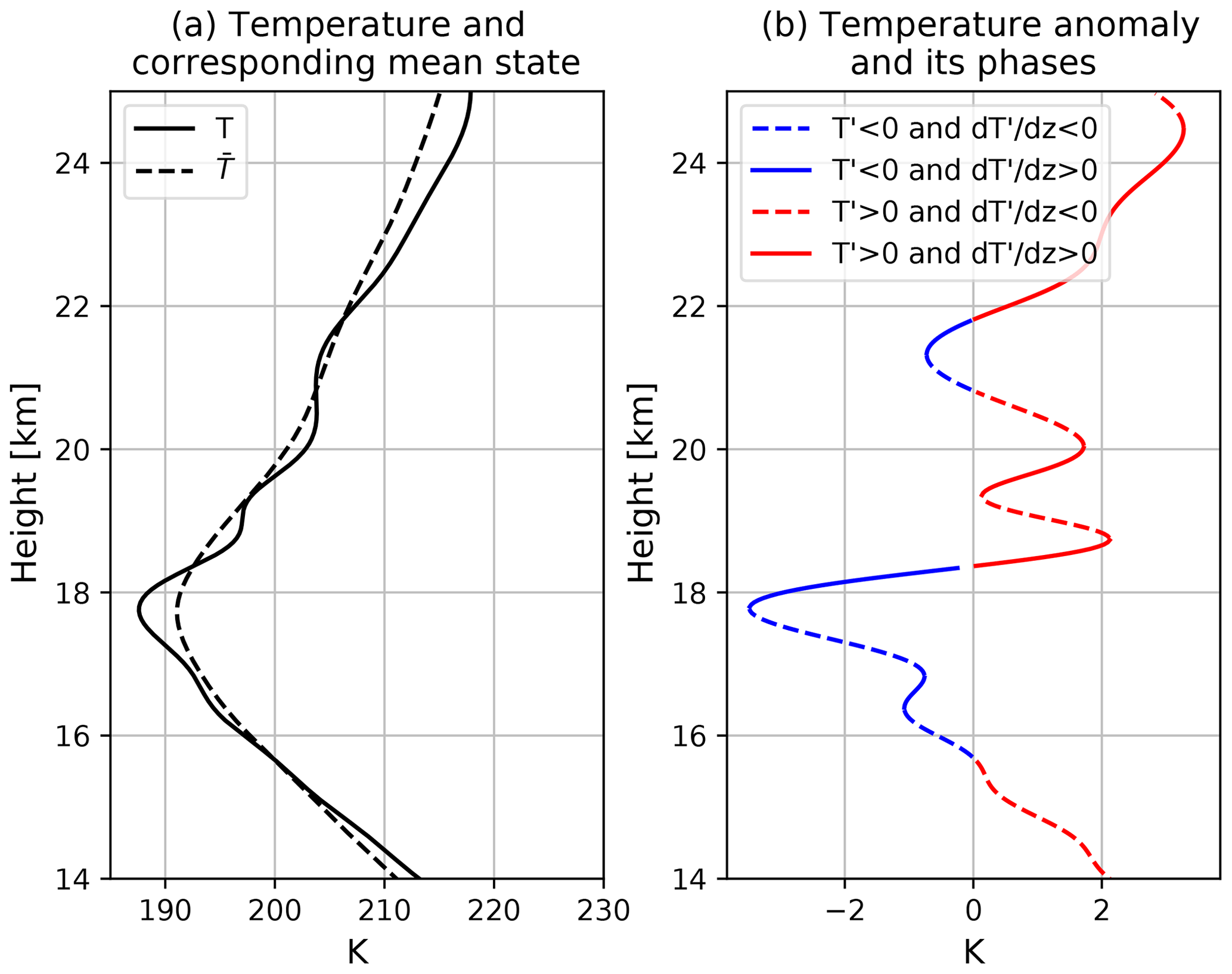
Figure 1 (a) Temperature profile (solid line) from COSMIC at 155^∘43^′ W, 18^∘16^′ N on 1 January 2007 and its corresponding mean state (dashed). (b) T^′ of the given profile and its four phases based on the sign of T^′ and $\text{d}{T}^{\prime }/\text{d}z$.

3.2 Collocation of CALIPSO observations with RO profiles

The primary goal of this work is to study cirrus occurrence and properties in the four gravity wave phases defined in Fig. 1. To accomplish this we collocate CALIPSO cloud observations with RO temperature profiles. The horizontal weighting of RO retrievals is mostly centered within 200 to 300 km of the perigee (tangent) point (Kursinski et al., 1997) where the ray experiences most bending. For this reason we use the spatial location of the perigee point as a basis for collocation. Since our interest lies strictly inside the TTL and the perigee point of each occultation ray changes with height, we determine the perigee point at the middle of the TTL by interpolating the longitude and latitude of RO profiles to 17.25 km (middle of TTL determined as the average of 14.5 and 20 km). Any CALIPSO observations within 100 km of this point are collocated with the RO profile for analysis. Figure 2 gives an example of one RO profile, its perigee point at 17.25 km, and the collocated CALIPSO 5 km footprints.

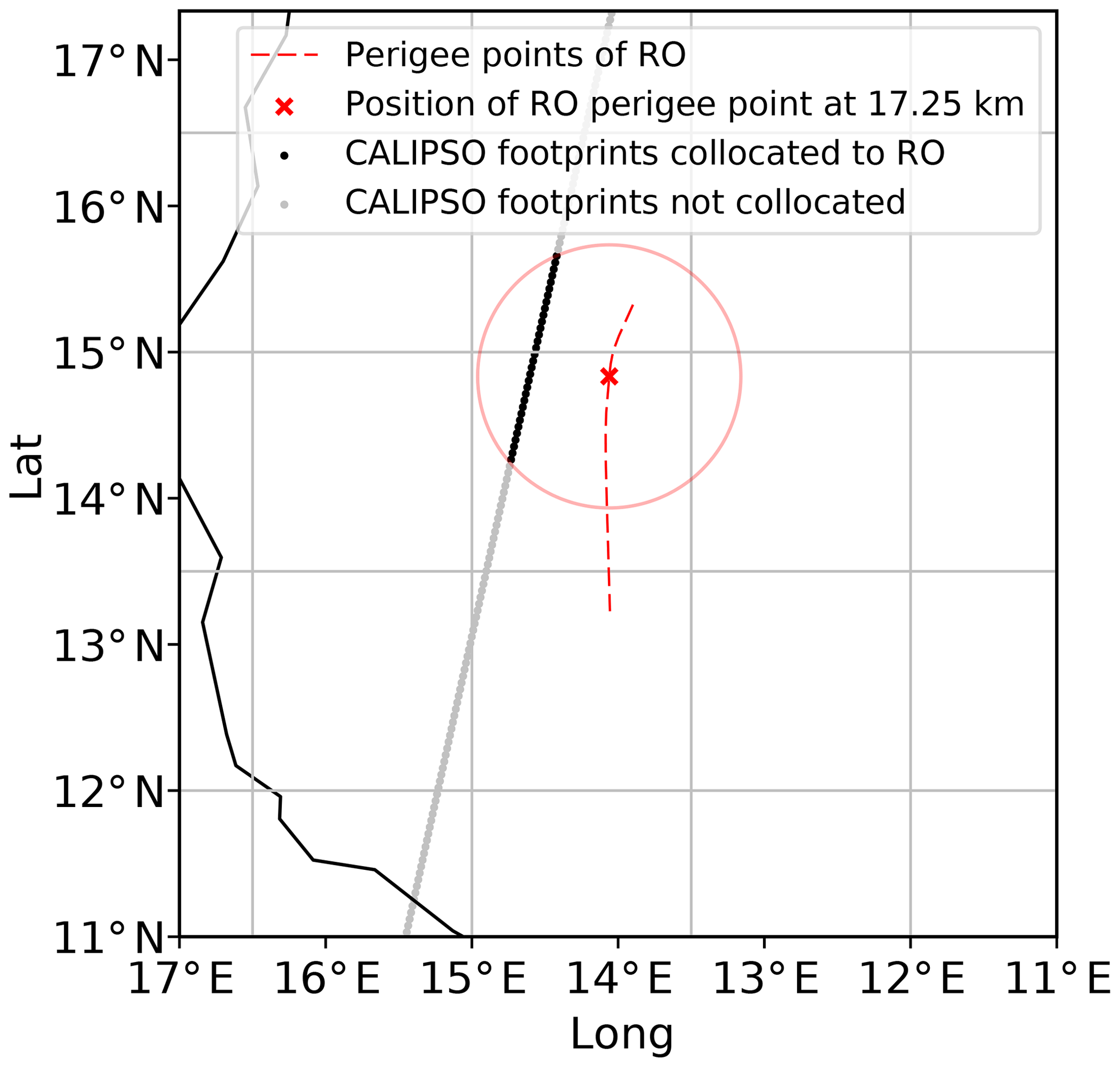
Figure 2 Schematic of collocation between RO profile and CALIPSO footprints. The perigee points of the RO profile throughout all altitudes are shown in the red dashed line, while the position of the perigee point in the middle of the TTL (17.25 km) is denoted by the red X. The CALIPSO 5 km product provides estimates of cloud properties at 5 km footprints, and all footprints within 100 km of the red X are collocated with the RO profile, as indicated by the black dots. Gray dots are CALIPSO footprints, considered too far from the RO profile and not collocated. The shown RO profile was taken at approximately 01:20 UTC on 2 January 2009.

We collocate RO profiles with 2C-ICE cloud retrievals in a similar manner. Unlike the CALIPSO 5 km products, 2C-ICE provides cloud properties at 1 km footprints and vertical bins of approximately 250 m. Other than this difference, the collocation method is identical to that of CALIPSO and RO. In May 2008 the Aura MLS was aligned to within ±10 km of CALIOP. For analysis involving RH_i, for each CALIPSO footprint with a RO collocation, we find the closest MLS footprint to that CALIPSO footprint to calculate RH_i.

4 Results

All results below were derived from data within 20^∘ of the Equator. For convenience we will refer to the four gravity wave phases as follows. Phase 1: $T^{\prime }<\mathrm{0}$ and $\text{d}{T}^{\prime }/\text{d}z<\mathrm{0}$; Phase 2: $T^{\prime }<\mathrm{0}$ and $\text{d}{T}^{\prime }/\text{d}z>\mathrm{0}$; Phase 3: $T^{\prime }>\mathrm{0}$ and $\text{d}{T}^{\prime }/\text{d}z<\mathrm{0}$; and Phase 4: $T^{\prime }>\mathrm{0}$ and $\text{d}{T}^{\prime }/\text{d}z>\mathrm{0}$. Cold and warm phases refer to where $T^{\prime }<\mathrm{0}$ and $T^{\prime }>\mathrm{0}$, respectively.

For the analysis presented in Sect. 4.1 and 4.3, the temporal restriction for collocation is that all the collocated data must be within 2 h of each other. This restriction is not imposed in Sect. 4.2, and the time difference between RO and CALIPSO observations ranges from 0 to 36 h with the purpose of examining how waves and cirrus clouds tend to evolve over time. This will be further elaborated in that section.

4.1 Population of clouds in wave phases

As previously mentioned, K16 (their Fig. 5) found that a majority of TTL clouds in the ATTREX data were observed in the cold phase $T^{\prime }<\mathrm{0}$ and that in the 2014 flight legs over the western Pacific there was a higher frequency of ice inside $\text{d}{T}^{\prime }/\text{d}z<\mathrm{0}$ than in $\text{d}{T}^{\prime }/\text{d}z>\mathrm{0}$. To assess whether this tendency is general throughout the TTL or is limited to the regions observed by ATTREX, we evaluate cloud populations using collocated CALIPSO and RO observations that cover the TTL at all longitudes and over 2007–2013. Figure 3 shows the population of CALIPSO Cloud Profile vertical bins detected as clouds in each wave phase extracted from collocated RO profiles. Considering all collocated observations between 1 January 2007 and 31 December 2013, 54.9 % of clouds are observed to occur in Phase 1 throughout the entire TTL, as shown in Fig. 3a. When the cloud population is examined in 1 km vertical layers (14.5–15.5 km, 15.5–16.5 km, etc.), there is no obvious change with height, and most clouds are found in Phase 1 followed by Phase 2 at all heights. Above 16.5 km there is a smaller fraction of clouds in the warm phase. A possible explanation for this may be that there are less convectively detrained clouds as altitude increases, increasing the probability of clouds having been formed by gravity waves. In addition, the population in Phase 2 tends to increase with height, with 38 % of clouds above 17.5 km in Phase 2. For comparison, using K16's Fig. 5 one can infer that for clouds above 16.5 km the cloud fractions in Phases 1, 2, 3, and 4 are 56.25 %, 31.25 %, 9.375 %, and 3.125 % (calculated as the percentage in that phase divided by the sum of all four phases), and for clouds below 16 km the percentages are 49.30 %, 28.17 %, 14.08 %, and 8.45 %. These ratios are similar to our findings, though we find fewer clouds in Phase 2 below 16 km. While the percentages in Fig. 3a are representative of the entire tropics, the above estimates based on K16's Fig. 5 are based on observations over the western Pacific. We split the tropics into smaller regions to facilitate better comparison.

Cloud fractions in each phase are separated into six longitudinal belts in Fig. 4. Filled bars represent the cloud fraction of all TTL clouds, while unfilled bars represent only clouds above the mean tropopause of their respective season and longitudinal belt. During December–January–February (DJF), the 120–180^∘ E belt, which covers the Maritime Continent and western Pacific, has the lowest cloud population in Phase 1 (51 %) as well as the most clouds inside the warm phase (24 %). Although this region is known for very low tropopause temperatures and high TTL cirrus frequency during DJF (Highwood and Hoskins, 1998; Sassen et al., 2009), there is also frequent deep convection (Ramage, 1968) which may generate clouds unrelated to gravity waves. This may explain the higher cloud population in warm phases. By eliminating clouds below the tropopause, above which convective detrainment is rare, the amount of cloud inside the warm phase in this region reduces to 10 %.

The influence of convection may also explain the high warm phase population during June–July–August (JJA) in 60–120^∘ E, where there is frequent convection due to the Asian summer monsoon. In this period and region, 28 % of clouds are in the warm phase and 47 % are in Phase 1. However, the reduction of cloud population in the warm phase after eliminating clouds below the tropopause is not as apparent here. One possible cause of this may be that the tropopause within 10 to 40^∘ N is elevated due to the Asian monsoon anticyclone in the upper troposphere, causing the tropopause to be more than 1 km higher than the zonal mean (Ploeger et al., 2015). Since our mean tropopause is calculated based on all profiles within 20^∘ N to 20^∘ S, some clouds from convective detrainment (especially those in the Northern Hemisphere) may still be included in the cloud population.

Over 180–120^∘ W, which approximately covers the eastern Pacific, 56 % (25 %) of clouds fall in Phase 1 (Phase 2) during DJF. This is in contrast with K16, who found that in the 2011 and 2013 ATTREX flight legs over the eastern Pacific there were slightly more clouds in Phase 2 than in Phase 1. The 2011 flights were conducted in October and November, while the 2013 flights were in February and March. Plots similar to Fig. 4 made from data in October–November (not shown) yielded Phase 1/2 populations of 64 %/23 %, while February–March yielded 57 %/20 %. Over this region we were not able to find Phase 2 having more clouds than K16 did. Their T^′ were calculated as the difference between aircraft in situ temperature and 30 d mean temperature derived from RO, while we calculate it as the difference between RO-derived temperatures and 7 d mean profiles. Reproducing the cloud population using 31 d mean temperature as the background still resulted in more clouds in Phase 1 than 2 (not shown). It is not clear what causes this difference.

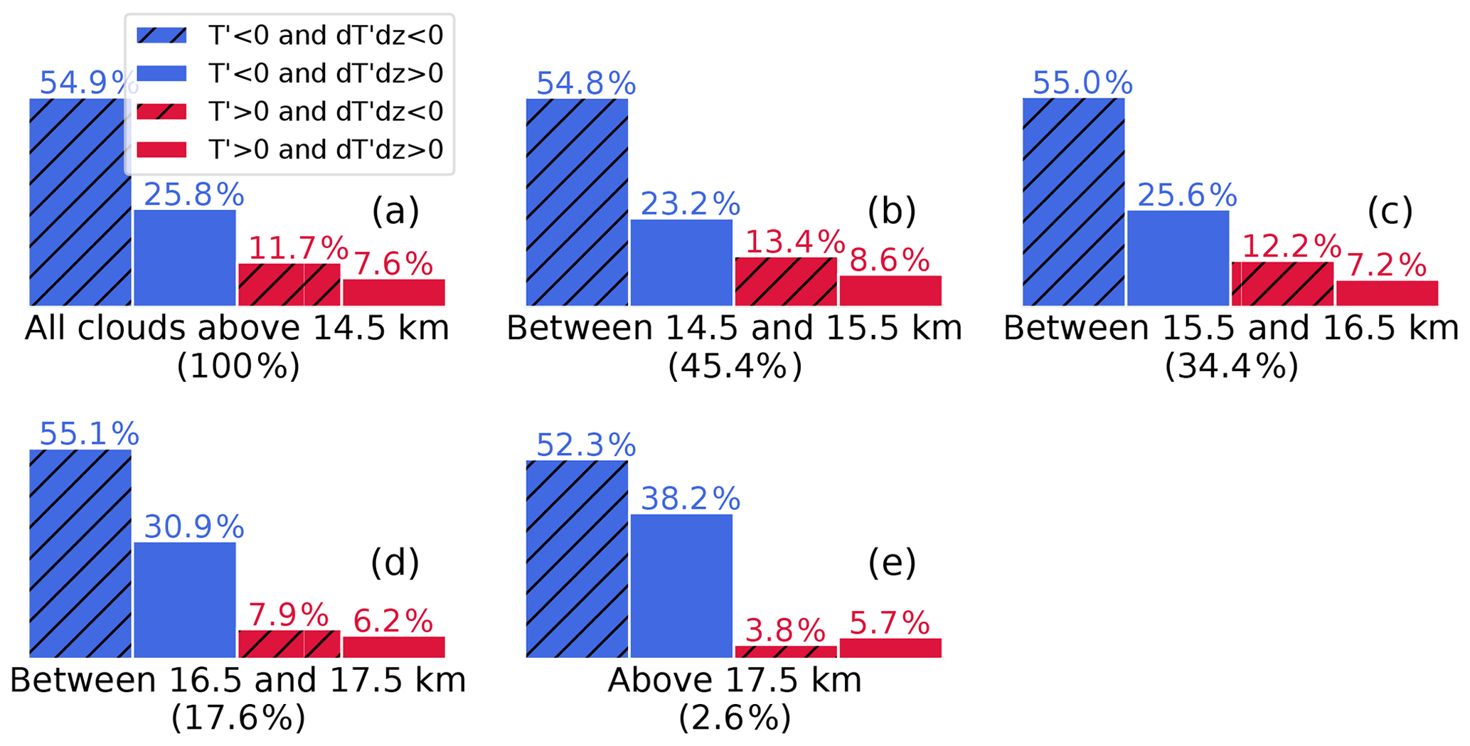
Figure 3 Population of CALIPSO Cloud Profile cloud bins inside each wave phase from 1 January 2007 to 31 December 2013. (a) shows the cloud population for all of TTL (14.5 to 20 km), while (b)–(e) show the population in four different 1 km layers. The percentage in parentheses denotes the portion of clouds found in that vertical layer relative to all TTL clouds.

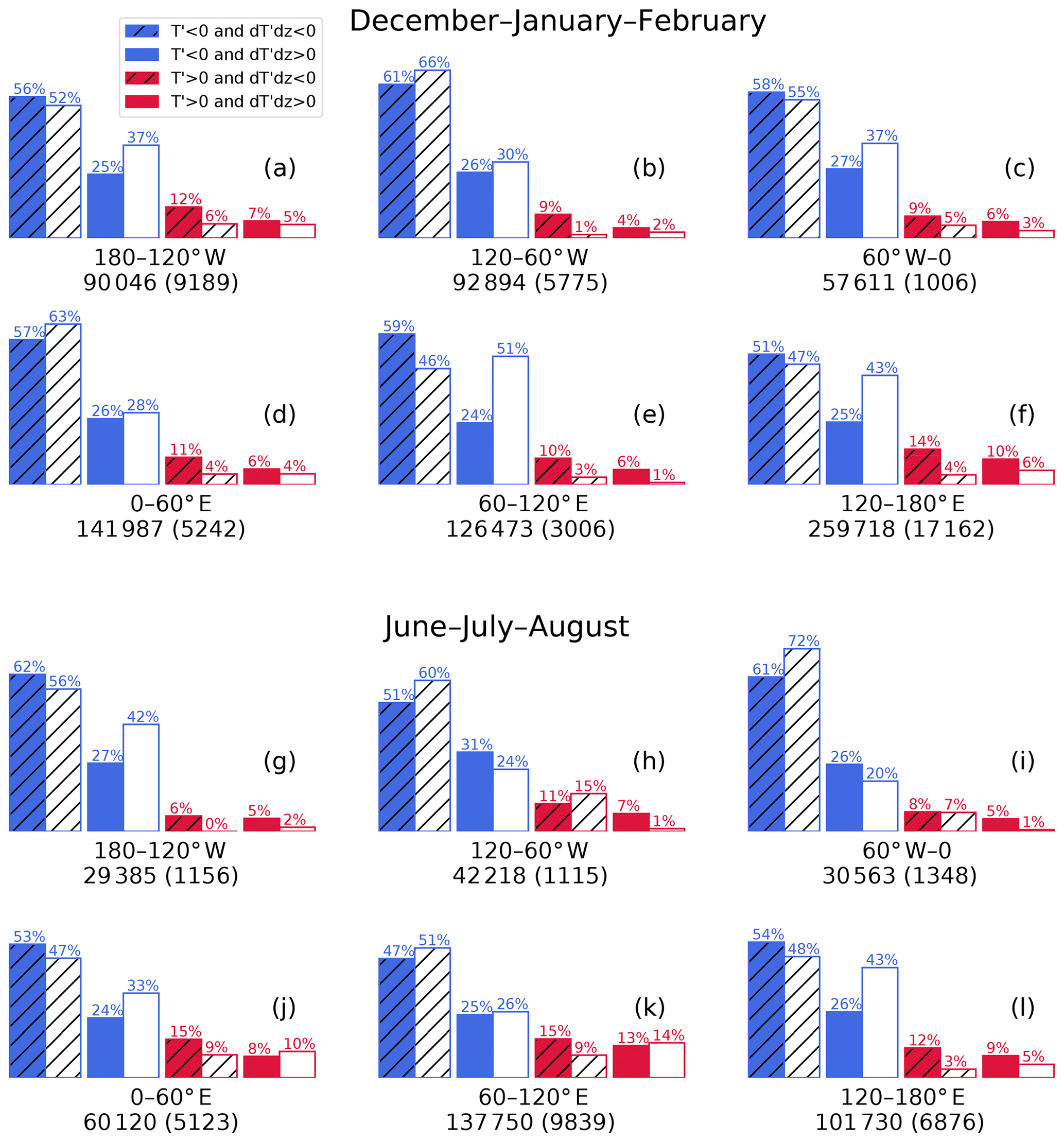
Figure 4 Same as Fig. 3a except for different longitudinal belts. (a)–(f) are for December–January–February and (g)–(l) are for June–July–August. Filled bars represent all TTL clouds, while unfilled bars represent only clouds above the mean tropopause of the respective longitudinal belt and season. The numbers of all cloud bins and bins above the tropopause (in parentheses) in each longitudinal belt are labeled under each bar plot.

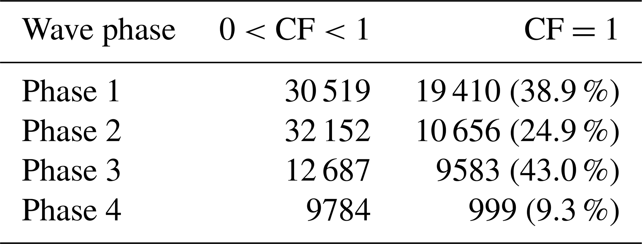
Using the cloud top and base heights reported from the CALIPSO Cloud Layer product, we calculate the cloud fraction in each wave phase, defined as the amount of vertical overlap between individual cloud layers and wave phases in Fig. 1. For example, if a phase layer occupies 15.0 to 16.0 km and the CALIPSO product reports a cloud layer extending from 15.2 to 15.7 km, then the cloud fraction would be 0.5. The cloud fraction of each observed wave phase is evaluated, and the resulting distributions of cloud fraction are shown in Fig. 5. In this figure we only consider clouds with base above 14.5 km and wave phase layers whose base height lies within 14.5 and 18.5 km. Note that cloud fractions of 0 and 1 are excluded in this figure. Corresponding to Fig. 5, the total sample number in each phase is shown in the first column of Table 1, while the number of cases with unity cloud fraction is shown in the second column.

In phases of positive $\text{d}{T}^{\prime }/\text{d}z$, the number of samples tends to decrease as cloud fraction increases. This trend does not apply for negative $\text{d}{T}^{\prime }/\text{d}z$, and in Phase 1 there is a clear increase in samples with increasing cloud fraction. In contrast, Phases 2 and 4 tend to have decreasing cloud fractions, while Phase 3 has a rather uniform distribution across all values. It is interesting that Phase 3 has a high percentage (43 %) of unity cloud fraction, much higher than Phase 4. Although both Phases 3 and 4 have a positive temperature anomaly, we find that Phase 3 seems to be much more favorable for clouds, consistent with P16's assertion that upward vertical wind anomaly is an important factor in maintaining ice clouds.

Figure 5 Distribution of cloud fraction in each gravity wave phase. Blue and red colored lines indicate the cold and warm phases, respectively, while the solid and dashed lines represent $\text{d}{T}^{\prime }/\text{d}z>\mathrm{0}$ and $\text{d}{T}^{\prime }/\text{d}z<\mathrm{0}$. The number of cases with cloud fractions of zero or unity are excluded.

Table 1 Number of cases with cloud fraction (CF) between 0 and 1 (sum of cases in Fig. 5) and CF = 1. The percentage represents the number of CF = 1 cases over the sum of the respective row.

4.2 Composite time evolution of wave anomalies and cirrus occurrence

Since COSMIC observations are pseudo-random in time and space, it is possible to collocate CALIPSO observations with RO soundings with varying offsets in time. By binning the temperature profiles according to the time offsets, we can make a composite showing the mean time evolution of wave anomalies relative to the cloud observation. Such an approach of creating composite time series has been used to study the thermodynamic budget before and after tropical convection (Masunaga, 2012; Masunaga and L'Ecuyer, 2014), temperature anomalies associated with tropical deep convection (Paulik and Birner, 2012), and the interaction between atmospheric dust and tropical convection (Sauter et al., 2019).

We bin RO profiles in time bins of −35, −33, …, −1, 1, …, 33, and 35 h relative to the CALIPSO observations, where a negative value indicates that the collocated RO profiles precede the CALIPSO overpass in time. The composites of T^′, $\text{d}{T}^{\prime }/\text{d}z$, and buoyancy frequency N² anomaly for all collocations in 2007 to 2013 are shown in Fig. 6. In making these composites we only include clouds with a cloud base of at least 14.5 km to ensure that the included clouds are TTL clouds (instead of, for example, convection). Also, for statistical testing, we need the RO profiles used in each time bin to be unique. For this reason, only the CALIPSO footprint spatially closest to the RO profile is used. If this is not done, then the same RO profile may be reused several times since there are usually multiple CALIPSO footprints collocated with one RO profile as shown in Fig. 2.

In Fig. 6a, the strongest cold anomaly is found close to the cloud top and is coldest near hour 0. The cold anomaly contour with a value below −0.8 K lasts approximately from −12 to +6 h and migrates downward with time, consistent with the property of gravity and Kelvin waves with upward group velocity. The alternating cold–warm anomaly at heights of +2 to +6 km should be due to the diurnal tide (Zeng et al., 2008; Pirscher et al., 2010) since we are compositing only on nighttime data from CALIPSO, which always crosses the equatorial region at similar local times. The number of samples in each time bin (Fig. 6c) has a 12 h periodicity mainly due to Metop-A/B. When only using COSMIC observations to reproduce Fig. 6a, b,and d, the anomaly patterns are largely the same, so the periodicity does not affect the composites.

It is noteworthy that the mean cold anomaly is centered near the cloud top and not within the cloud. This results in a dipole structure in $\text{d}{T}^{\prime }/\text{d}z$ (Fig. 6b) and buoyancy frequency anomaly (Fig. 6d) with positive anomalies just above the cloud top and negative anomalies below. This structure shows that the inside of clouds (below cloud top) is likely to have negative $\text{d}{T}^{\prime }/\text{d}z$, consistent with the finding by K16 and Fig. 3 that a majority of clouds are found in Phase 1. Although this structure implies weakened stability (negative N² anomaly) inside the cloud, it is unclear whether this decreased stability has connections to cloud formation or maintenance. Since negative $\text{d}{T}^{\prime }/\text{d}z$ also corresponds to upward vertical motion anomalies (assuming that these anomalies are from gravity waves), their effects are difficult to separate.

A prediction of P18 is that the ice sedimentation velocity is comparable to the gravity wave vertical phase speed. In Fig. 6, the descent rate of the cold anomaly within −12 to +6 h is about 1 km over 18 h. Assuming a spherical ice crystal with a radius of 15 µm and an ambient temperature of 200 K, P18's equation (20) (valid for radii in 5–100 µm) yields a sedimentation velocity of ∼ 2 cm s⁻¹. This corresponds to a displacement of ∼ 1.3 km over 18 h, which is comparable to the vertical descent rate of the cold anomaly.

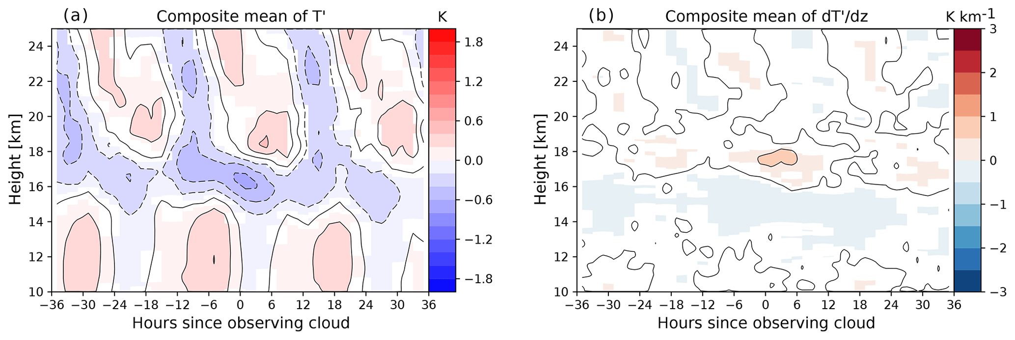
Figure 7 is similar to Fig. 6 except that the anomalies are not composited relative to the cloud top height, but rather on height above mean sea level. In this composite, there are cold anomalies at TTL altitudes, but the magnitude is weaker than that of Fig. 6. This leads to weak anomalies in $\text{d}{T}^{\prime }/\text{d}z$ (Fig. 7b) and N² (not shown). Based on these results we suggest that gravity wave anomalies in Fig. 6 are physically significant and have a close association with the vertical position of TTL cloud tops.

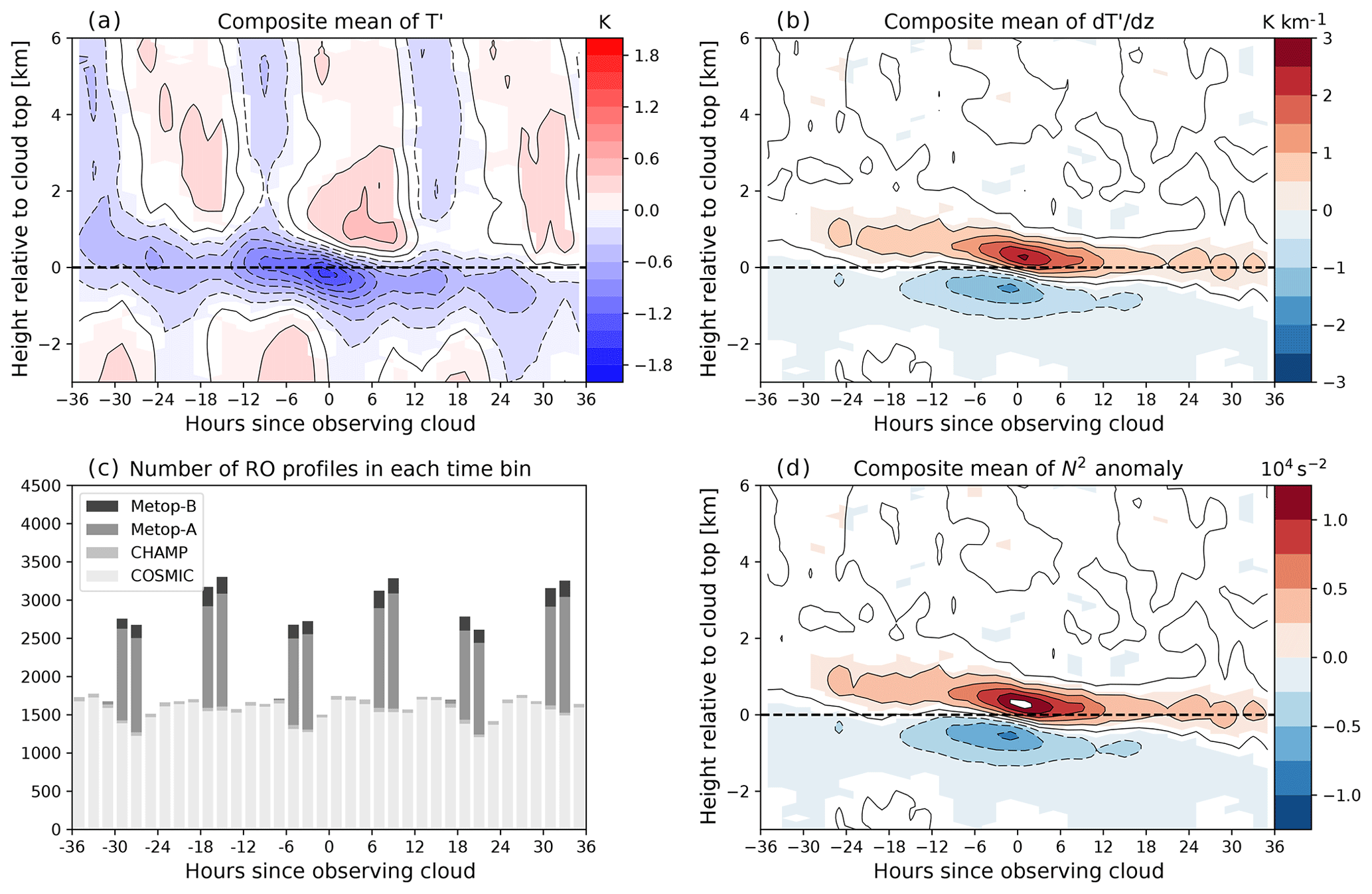
Figure 6 Composite of (a) T^′, (b) $\text{d}{T}^{\prime }/\text{d}z$, and (d) buoyancy frequency N² anomaly in height coordinate relative to cloud top. Colored contours in these three plots are at or above the 95 % significance level according to the Student's t test. Solid (dashed) contours represent positive (negative) anomalies and are at the same levels as the colored contours. The abscissa denotes the time offset between the CALIPSO observation and RO sounding. (c) shows the number of unique RO profiles in each 2 h time bin used to calculate the composites.

Figure 7 Composites of (a) T^′ and (b) $\text{d}{T}^{\prime }/\text{d}z$ based on height above mean sea level (instead of height coordinate relative to cloud top as in Fig. 6). Colored contours are at or above the 95 % significance level according to the Student's t test. Contour levels are identical to Fig. 6.

P18 argue that the upward vertical velocity in Phase 1 slows down the descent of ice crystals and tends to suspend them inside Phase 1. Since these composites depict a downward propagation of wave anomalies, it is of interest to investigate whether the phase propagation of gravity waves is associated with a downward migration of clouds. We can explore this possibility through a compositing technique similar to the one employed above. Instead of centering on the CALIPSO footprint, we center on the time of RO sounding and use the CALIPSO cloud product to calculate the cloud frequency in each 2 h time bin. In addition, instead of compositing relative to cloud top height, we composite on the altitude of the local minima or maxima of T^′. A schematic of this compositing approach is given in Fig. 8.

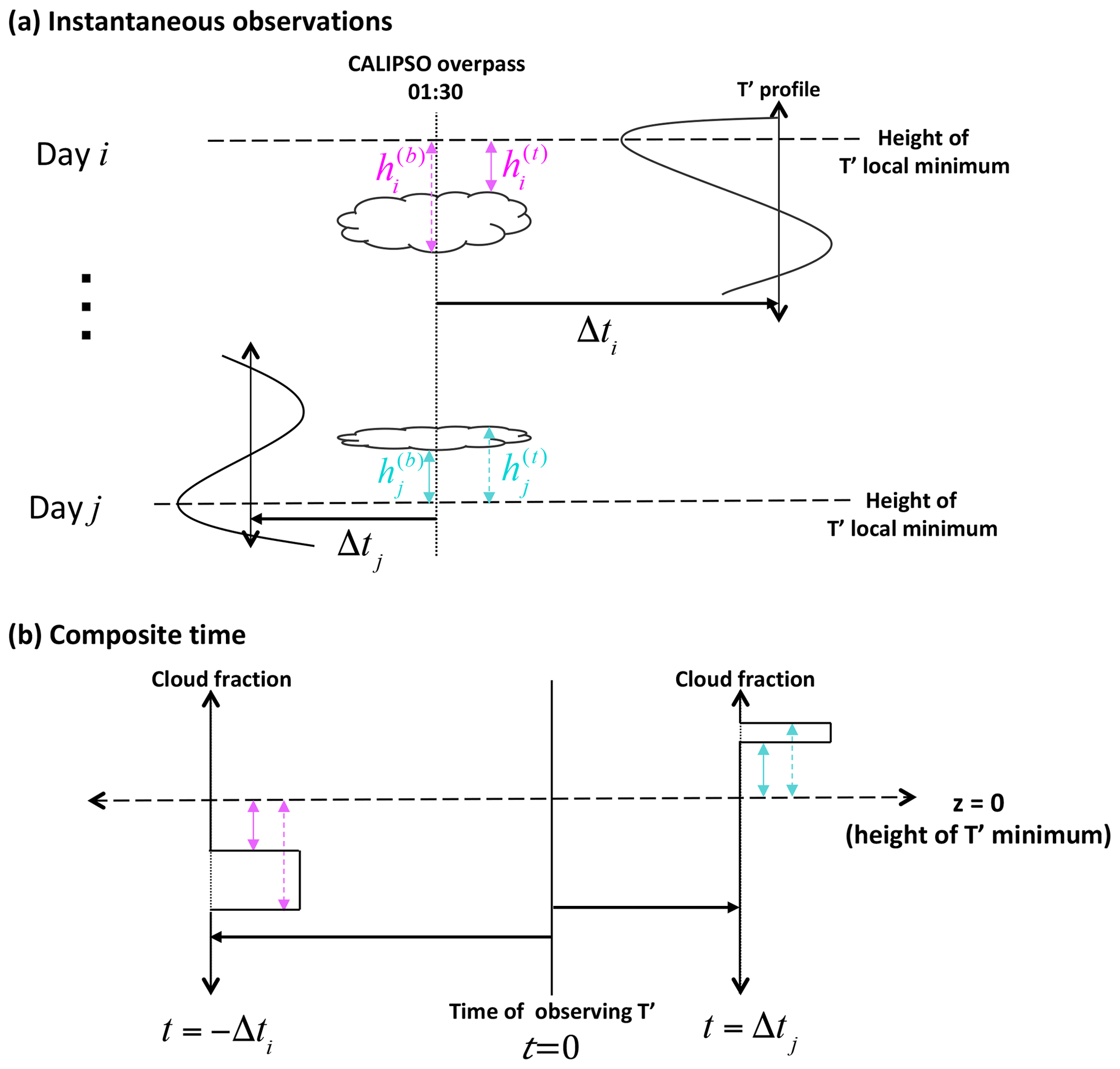
Figure 8 Schematic for creating the composite temporal evolution of cloud fraction with respect to T^′ minima. In this example, as shown in (a), during day i there is a collocated pair of CALIPSO and RO observations. The RO observation occurs Δt_i hours after that of CALIPSO, and the vertical distance between the height of local T^′ minimum and the cloud top and base is depicted by the dashed and solid magenta lines, respectively, with lengths $h_i^{\left(t\right)}$ and $h_i^{\left(b\right)}$. In the temporal compositing (b), in the time bin corresponding to Δt_i hours before observing T^′, the cloud fraction is binned according to how much each vertical bin overlaps with the interval $[h_i^{\left(b\right)},h_i^{\left(t\right)}]$. The same procedure is carried out for the collocated pair at day j. Also see text for explanation.

In the example shown in Fig. 8a, at day i there is a collocated RO sounding that occurred within 100 km of the CALIPSO footprint but Δt_i hours after. The position of the cloud top and base (solid and dashed magenta lines) is evaluated relative to a local T^′ minimum. Since the CALIPSO overpass occurred before this RO profile, in the compositing (shown in Fig. 8b) the observed cloud position is used to calculate the cloud fraction at Δt_i hours before the RO sounding. The cloud fractions are calculated on a grid of 50 m height and 2 h time bins. For the collocation pair in Fig. 8a, the cloud fraction in the time bin corresponding to $t=-\mathrm{\Delta }{t}_i$ is calculated according to how much each vertical bin overlaps with the interval $[h_i^{\left(b\right)},h_i^{\left(t\right)}]$. If the collocated CALIPSO footprint has no clouds with a base above 14.5 km, cloud fractions of zero are still binned in the appropriate time bin at all heights. Since any RO profile most likely has multiple local minima, the binning of cloud fraction is repeated for each local minimum in a T^′ profile. The exact same procedure is conducted for local maxima to create a separate cloud frequency composite. To focus on TTL clouds we only include clouds with a base at or above 14.5 km. Also, we only consider local T^′ extrema within 14.5 to 18.5 km since a majority of TTL clouds are inside this height range.

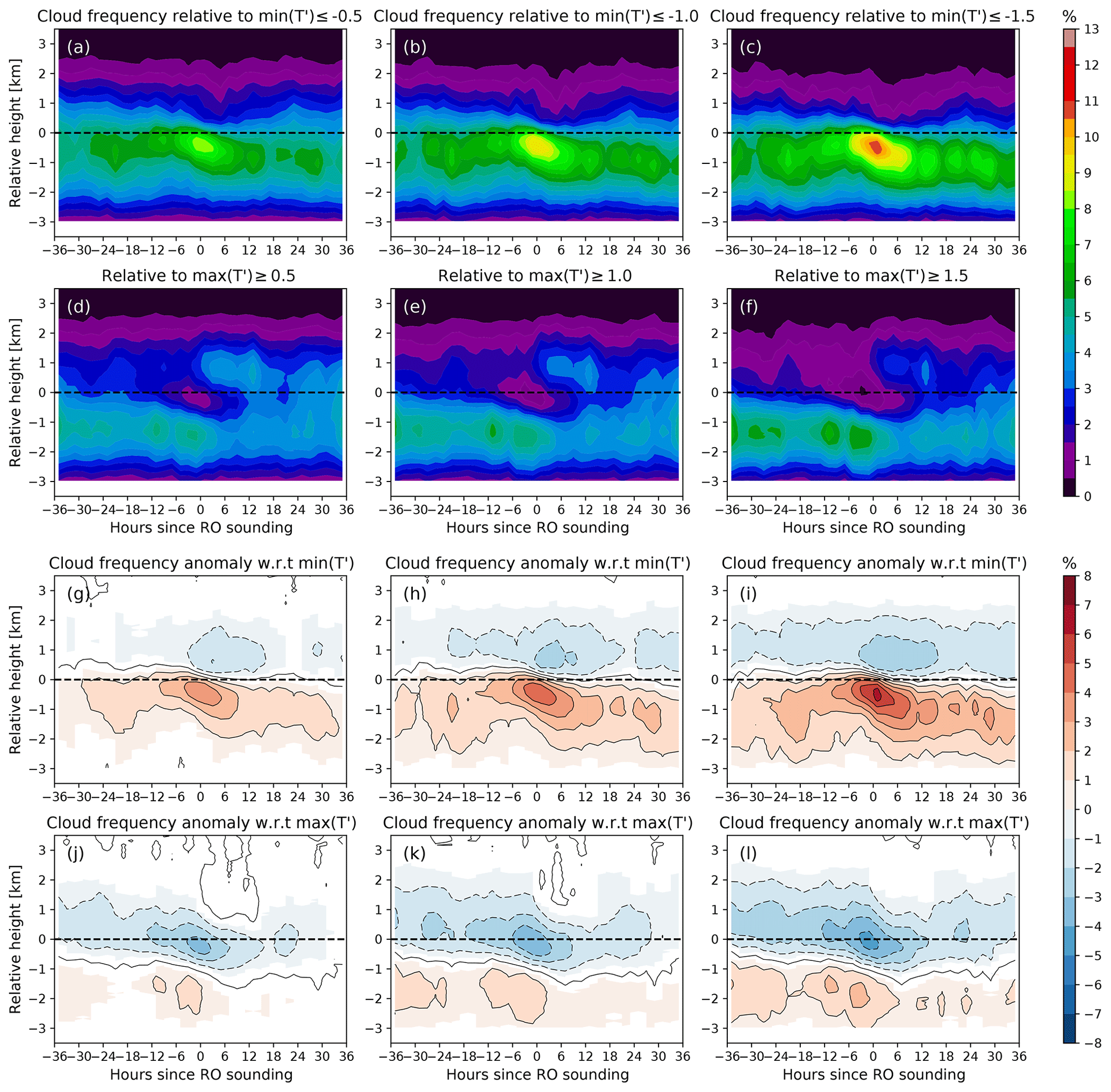
Figure 9 Composite of cloud frequency with respect to local minima (first row; panels a–c) or maxima (second row; panels d–f) of T^′. The columns correspond to composites made from subsets of T^′ extrema with magnitudes greater than or equal to 0.5 K (left column), 1.0 K (middle), and 1.5 K (right). Dashed horizontal lines indicate the position of the local T^′ extrema. The third row (g–i) and fourth row (j–l) are the cloud frequency anomalies associated with cold or warm anomalies, respectively. Contours in the bottom two rows are at intervals of 1 % (dashed negative), matching the filled color contours which show values at or above the 95 % significance level.

The composites of cloud frequency made this way, shown in Fig. 9a–c and d–f, can then be interpreted as the probability of finding clouds in the vicinity of local T^′ minima or maxima, respectively. The shown values represent the mean cloud fraction in each time–height bin. Each column is produced from a different subset of T^′ extrema based on magnitude ($\left|T^{\prime }\right|>\mathrm{0.5}$, 1.0, or 1.5 K). Beneath the vertical position of $min\left(T^{\prime }\right)$ (Fig. 9a–c) we find a lobe of enhanced cloud frequency, and this becomes more evident as $min\left(T^{\prime }\right)$ decreases. Likewise, in the vicinity of $max\left(T^{\prime }\right)$ (Fig. 9d–f) the cloud frequency is reduced, and this reduction also shows dependence on the magnitude of $max\left(T^{\prime }\right)$. In both cases, the increased or decreased cloud frequency displays a downward trend consistent with the expectation that gravity wave phases propagate downward with time. We devise a way to extract the cloud frequency anomaly associated with these patterns; the method and the statistical testing are detailed in the Appendix. To summarize the method briefly, we produce a background cloud frequency and compare it with the pattern shown in Fig. 9a–c and d–f to find statistically significant values through the Kolmogorov–Smirnov test (K–S test) (Hollander et al., 2015).

Figure 9g–i are the anomalies associated with $min\left(T^{\prime }\right)$, and similarly panels (j)–(l) show the anomalies associated with $max\left(T^{\prime }\right)$. Colored portions of the contour denote regions with p<0.05 (95 % confidence) as estimated from the K–S test. In these anomaly patterns it is confirmed that there is enhanced cloud occurrence below $min\left(T^{\prime }\right)$, and, in addition, a weak reduction of cloud occurrence above it. For the subset of $min\left(T^{\prime }\right)<-\mathrm{0.5}$, the positive cloud frequency anomaly peaks at 3 %, whereas for $min\left(T^{\prime }\right)<-\mathrm{1.5}$ it peaks at 6 %. The anomaly patterns due to $max\left(T^{\prime }\right)$ also exhibit a dipole structure with negative anomalies centered on the altitude of $max\left(T^{\prime }\right)$ and a weak positive anomaly below. Panels (j)–(l) also suggest a dependence of cloud frequency anomaly on the magnitude of $max\left(T^{\prime }\right)$, although the variation is not as large compared to that of $min\left(T^{\prime }\right)$. Both positive/negative anomalies associated with $min\left(T^{\prime }\right)/max\left(T^{\prime }\right)$ tend to migrate downward in time, although this trend is slightly more apparent in the enhanced cloud occurrence of $min\left(T^{\prime }\right)$.

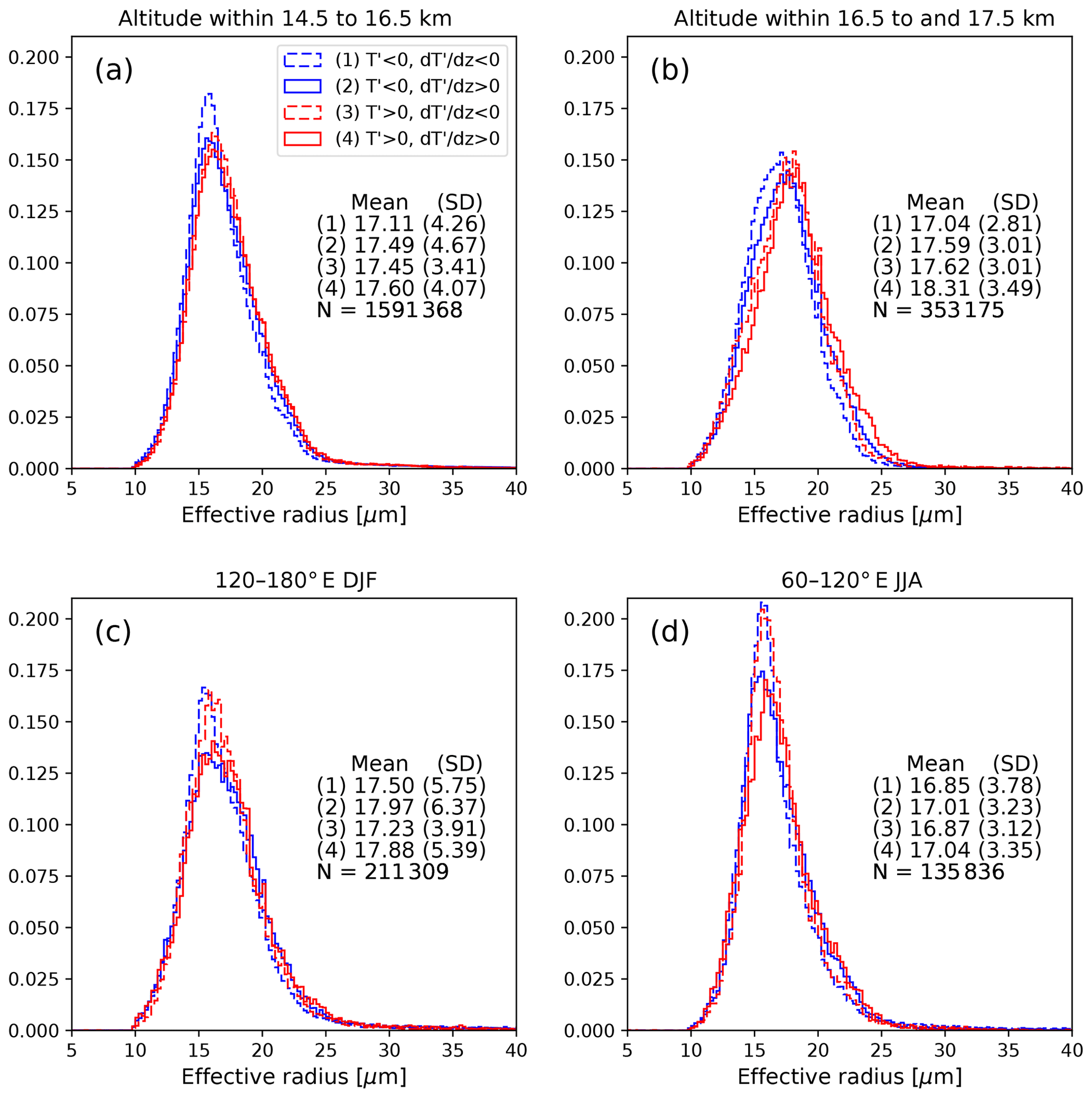
Figure 10 Normalized density function of r_e in each gravity wave phase for clouds within (a) altitudes of 14.5 to 16.5 km, (b) 16.5 to 17.5 km, (c) 120–180^∘E in December–January–February, and (d) 60–120^∘E in June–July–August. The mean and standard deviation (SD) of r_e in each phase and the total number of r_e samples (N) are denoted in the legend.

One difference between $min\left(T^{\prime }\right)$ and $max\left(T^{\prime }\right)$ is that the positive anomalies in $min\left(T^{\prime }\right)$ occur below the altitude of $min\left(T^{\prime }\right)$, while the negative anomalies in $max\left(T^{\prime }\right)$ are centered on it. This suggests that most of the enhanced cloud occurrence occurs inside Phase 1, and Phase 2 actually tends to have a negative cloud occurrence anomaly. Although the predictions of P18 suggest that it may be more likely to find clouds in Phase 2 under low background RH_i, this global analysis suggests that on average the role of Phase 1 in facilitating TTL clouds is dominant.

4.3 Comparison to P18

P18 suggests that (1) ice crystals within a confined range of r_e are suspended in Phase 1, and (2) for low background relative humidity with respect to ice (RH_ib), the region of confinement may overlap with both Phase 1 and Phase 2, with its center still inside Phase 1 but closer to Phase 2. These two features are depicted in their Fig. 2. To evaluate whether these predictions are consistent with satellite observations, we examine r_e and RH_ib in observations to see whether these quantities exhibit any correlations with clouds in each gravity wave phase. Although here we present analysis motivated by P18, we note that their study assumes no background wind shear in their derivations and simulations.

Figure 10 shows normalized distributions of r_e in the four wave phases as well as their means and standard deviations. These distributions only contain nighttime 2C-ICE data, since the information on thin cirrus is mostly from lidar backscatter. Clouds above 17.5 km were omitted in this plot due to the low samples (∼ 0.6 % of all TTL clouds). For clouds within 14.5–16.5 km (Fig. 10a), the r_e distribution of Phase 1 has a peak near 16 µm. Above 16.5 km (Fig. 10b) this peak is not evident, but the Phase 1 distribution has higher values around 15 µm and lower values between 20 and 25 µm, slightly differentiating Phase 1 from the other phases. In panels (a) and (b) the mean r_e of Phase 1 is lower than all three other phases, but the differences are small.

In Fig. 10c and d we examine two regions that are likely to be influenced by convection as inferred from Fig. 4. One may have expected these regions to have more convectively detrained clouds and therefore larger mean r_e, but this is not observed here; the mean r_e in panel (c) tends to be larger than panels (a) and (b), but this is not the case for panel (d). The influence of convection on r_e is not obvious, though we see that the r_e distributions of Phase 3 tend to resemble those of Phase 1 in these regions/seasons. The r_e distributions in panel (c) are notably wider (i.e., higher standard deviation) than the other categories, but the cause of this is not known.

In summary, our analysis of r_e shows that for the entire TTL (Fig. 10a and b), the observed characteristics of r_e show qualitative consistency with P18's findings, as Phase 1 tends to have slightly larger numbers of ice particles localized around a certain r_e value. On the other hand, the influence of convection is not apparent. We note that retrieving cloud properties of thin cirrus has large uncertainties, and more research is needed to explore the r_e distribution in gravity wave phases using a variety of observations and models.

As discussed in Sect. 4.1, K16 found that in the 2011 and 2013 flight legs over the eastern Pacific there were slightly more clouds in Phase 2 than in Phase 1, whereas in the 2014 flights over the western Pacific a majority of clouds were in Phase 1. P18 argue that this may be due to the relatively low RH_ib characteristic of the TTL over the eastern Pacific. P18 solved a simplified set of equations describing the interaction between gravity wave perturbations and ice particle growth/sedimentation. Comparison of their solution using values of RH_ib=0.85 or 0.63 (to represent the western and eastern Pacific, respectively) showed that the former results in the ice crystals being suspended in Phase 1, where in the latter ice particles were situated closer to the T minimum so that ice crystals were moving around between Phases 1 and 2. Motivated by these results, we collocate the MLS water vapor retrieval with CALISPO and RO data to evaluate whether observations suggest a similar dependence on RH_ib.

For each CALIPSO Cloud Profile bin identified as cloud, the collocated water vapor mixing ratio from the Aura MLS product is log-interpolated (as suggested by the product documentation) with the height of the cloud bin. To evaluate the saturation mixing ratio, we interpolate the 7 d mean temperature to the cloud height since we are interested in the RH_ib instead of the actual RH_i (which would include wave influence). The Goff–Gratch equation (Goff and Gratch, 1946) is used to get the saturation vapor pressure and subsequently the saturation mixing ratio and RH_ib. Then the cloud bin is binned according to RH_ib into bins of 0 %, 50 %, and then every 10 % up to 180 %. The first bin is wider due to the small amount of samples with very low RH_ib. Figure 11 shows the cloud population in each phase as a function of RH_ib as well as the number of cloud bins in each RH_ib category. Compared to the relative humidity observed during the ATTREX campaign (Jensen et al., 2017), the values in our Fig. 11 tend to be high-biased. A possible cause of this is that we are estimating the relative humidity as coarse-resolution MLS mixing ratio estimates divided by the saturation mixing ratio of the mean temperature. Due to the nonlinearity of the Goff–Gratch equation, the relative humidity evaluated this way will be larger than the actual average relative humidity.

Qualitatively, Fig. 11 is consistent with P18 since the Phase 2 percentage is higher when RH_ib is below 100 %. The percentage of clouds in Phase 1 also tends to increase with RH_ib up until RH_ib=100 %, above which there is no appreciable trend with RH_ib in any of the phases. To summarize, our analysis of RH_ib is consistent with P18's findings, while the results pertaining to r_e remain ambiguous.

Figure 11 (a) Percentage of TTL clouds inside each wave phase as a function of background relative humidity with respect to ice (RH_ib). (b) Number of CALIPSO Cloud Profile bins in each RH_ib category.

5 Conclusions

This study uses multiple satellite data sets to evaluate the influence of gravity wave perturbations on TTL cirrus clouds. With a focus on understanding the role of $\text{d}{T}^{\prime }/\text{d}z$, the vertical gradient of the gravity wave temperature perturbation T^′, we extract T^′ and $\text{d}{T}^{\prime }/\text{d}z$ from RO observations and collocate them with clouds observed by CALIPSO and 2C-ICE to understand cloud occurrence and characteristics in distinct wave phases. Similar to the results of K16, we find that the phase where T^′ and $\text{d}{T}^{\prime }/\text{d}z$ are both negative (Phase 1) is most frequently occupied by TTL clouds. The second most populous phase is where $T^{\prime }<\mathrm{0}$ and $\text{d}{T}^{\prime }/\text{d}z>\mathrm{0}$ (Phase 2), followed by where $T^{\prime }>\mathrm{0}$ and $\text{d}{T}^{\prime }/\text{d}z<\mathrm{0}$ (Phase 3) and then $T^{\prime }>\mathrm{0}$ and $\text{d}{T}^{\prime }/\text{d}z>\mathrm{0}$ (Phase 4). We show that this relation among the four phases is more or less invariant with height or longitude.

A mean view of the temporal evolution of wave anomalies with respect to clouds is constructed by taking advantage of RO's pseudo-random distribution in time and space. We collocate CALIPSO cloud observations with RO soundings that occur before and after the CALIPSO observation, and by averaging a large number of observations with different time separations, a composite time series of wave anomalies is presented. These composites show that, on average, the strongest cold anomaly due to gravity waves tends to be centered on the height of cloud top, and this cold anomaly descends with time consistent with the downward phase propagation of gravity and Kelvin waves with upward group velocity.

In the cloud frequency composites made with respect to local T^′ minima or maxima, we find that the decrease in cloud probability in the warm phase does not show clear dependence on the sign of $\text{d}{T}^{\prime }/\text{d}z$. This is distinct from the cold phase, where cloud probability is increased mainly below $min\left(T^{\prime }\right)$, where $\text{d}{T}^{\prime }/\text{d}z$ is negative. Together with existing studies, this result adds support to the idea that Phase 1 facilitates cloud formation and/or maintenance. Although the downward migration of the increased cloud frequency may be due to ice sedimentation, this is unlikely to be the case for the decreased cloud frequency associated with the warm phase. Hence the downward migration of increased/decreased cloud frequency in the temporal composites is most likely due to waves with downward phase propagation. We also show that the positive or negative cloud frequency anomalies strengthen with increasing magnitude of T^′ minima or maxima, giving evidence on a global scale that the wave amplitude is connected to the probability of cloud occurrence.

Finally, using satellite estimates of r_e from 2C-ICE, we assess the predictions of P18, which implies that one may observe a narrower distribution ice crystal effective radius inside Phase 1. Their conclusion that the background relative humidity with respect to ice affects the vertical position of clouds is also evaluated here by using RH_ib based on the Aura MLS H₂O product. Among all phases, r_e are distributed similarly, but the distribution of Phase 1 had a notably sharper peak than the other three phases and also a slightly smaller mean r_e. The partitioning of cloud population among the four phases showed clear dependence on RH_ib, with Phase 1's cloud population increasing with RH_ib up until RH${}_{\text{ib}}=\sim \mathrm{100}$ %. Overall, our satellite-based analysis shows qualitative consistency with the results of P18. This study adds to the literature showing that Phase 1 has a distinct connection to TTL clouds. The findings of K16, based on aircraft data limited to specific regions and time span, have been extended by our study, which shows that the large amount of clouds in Phase 1 is a general characteristic of the TTL. Based on our composite analysis using satellite data spanning 7 years (2007–2013), the connection between wave anomalies and cloud occurrence is evident: cold anomalies are associated with the position of cloud top, and T^′ amplitudes influence the increase or decrease in cloud frequency. The purpose of constructing composite temporal evolution by piecing together collocated temperature and cloud observations is an attempt to study processes occurring on a timescale typically unobserved by satellites. Although the resulting composites are not true time series, the anomaly patterns are consistent with wave propagation and enhance our understanding of how waves are connected to TTL clouds. It should be noted that although the composite technique shows a clear connection between wave anomalies and clouds, the technique is stationary in space; it does not follow the position of clouds (moved by the background flow) or the wave phase (moved as it propagates).

Due to the spatial and vertical resolution of the RO technique, the waves analyzed here have relatively large vertical wavelengths and low frequencies. The vertical wavelength inferred from the anomalies in our composites is about 3 km. Dzambo et al. (2019) showed that the power spectrum of TTL gravity waves tends to peak at wavelengths of around 4–5 km, though at 3 km there is still considerable power (their Fig. 1). These wavelengths are all resolvable by RO, so it can be assumed that this analysis has included a large part of the TTL gravity wave spectrum. Nevertheless, it remains to be explored whether Phase 1 of high-frequency waves is also distinct from other phases.

Appendix A: Calculation of background cloud frequency for Fig. 9

The cloud frequency composites in the top two rows of Fig. 9 are made using the altitude of the T^′ extrema as the zero height. To generate a composite where the vertical position of T^′ extrema has no relationship with cloud top/base height, for each T^′ extremum we generate a random altitude using uniform distribution unif(14.5,18.5) and make a separate cloud frequency time–height composite with the random altitude as zero height. The resulting cloud frequency height–time distribution is regarded as the “background” distribution. The difference between this background and the cloud frequency composites in Fig. 9a–f are then the anomalies associated with local T^′ minimum or maximum. The anomalies derived in this way are shown in Fig. 9g–l.

The distribution of cloud fraction in each time–height bin is similar to those shown in Fig. 5 and therefore is not normal, so the Student's t test cannot be used for statistical testing. We use the two-sided two-sample Kolmogorov–Smirnov test which does not make any assumptions about the data distributions. This test can be used to evaluate whether two discrete probability distributions differ from each other. The null hypothesis is that the cloud frequency pattern composited on T^′ minima/maxima (first/second row of Fig. 9) is not different than the randomly generated “background” cloud frequency pattern.