the Creative Commons Attribution 4.0 License.
the Creative Commons Attribution 4.0 License.
 | 11 Apr 2019
Satellite-derived sulfur dioxide (SO2) emissions from the 2014–2015 Holuhraun eruption (Iceland)
Elisa Carboni
Tamsin A. Mather
Anja Schmidt
Roy G. Grainger
Melissa A. Pfeffer
Iolanda Ialongo
Nicolas Theys
The 6-month-long 2014–2015 Holuhraun eruption was the largest in Iceland for 200 years, emitting huge quantities of sulfur dioxide (SO2) into the troposphere, at times overwhelming European anthropogenic emissions. Weather, terrain and latitude made continuous ground-based or UV satellite sensor measurements challenging. Infrared Atmospheric Sounding Interferometer (IASI) data are used to derive the first time series of daily SO2 mass present in the atmosphere and its vertical distribution over the entire eruption period. A new optimal estimation scheme is used to calculate daily SO2 fluxes and average e-folding time every 12 h. For the 6 months studied, the SO2 flux was observed to be up to 200 kt day−1 and the minimum total SO2 erupted mass was 4.4±0.8 Tg. The average SO2 e-folding time was 2.4±0.6 days. Where comparisons are possible, these results broadly agree with ground-based near-source measurements, independent remote-sensing data and values obtained from model simulations from a previous paper. The results highlight the importance of using high-resolution time series data to accurately estimate volcanic SO2 emissions. The SO2 mass missed due to thermal contrast is estimated to be of the order of 3 % of the total emission when compared to measurements by the Ozone Monitoring Instrument. A statistical correction for cloud based on the AVHRR cloud-CCI data set suggested that the SO2 mass missed due to cloud cover could be significant, up to a factor of 2 for the plume within the first kilometre from the vent. Applying this correction results in a total erupted mass of 6.7±0.4 Tg and little change in average e-folding time. The data set derived can be used for comparisons to other ground- and satellite-based measurements and to petrological estimates of the SO2 flux. It could also be used to initialise climate model simulations, helping to better quantify the environmental and climatic impacts of future Icelandic fissure eruptions and simulations of past large-scale flood lava eruptions.
- Article
(4014 KB) - Full-text XML
-
Supplement
(25936 KB) - BibTeX
- EndNote


Sulfur dioxide (SO2) is one of the most important magmatic volatiles for volcanic geochemical analysis and hazard assessments due to its low ambient concentrations, abundance in volcanic plumes and spectroscopic features. Tropospheric volcanic SO2 and its conversion products can affect the environment, human health, air quality and the radiative balance of the Earth (Schmidt et al., 2015; Gíslason et al., 2015; Schmidt et al., 2012; Gettelman et al., 2015; Ilyinskaya et al., 2017; Boichu et al., 2016; McCoy and Hartmann, 2015; Malavelle et al., 2017). Measurements of SO2 from volcanic eruptions are vital, both to understanding the underlying volcanic processes and also the wider-scale environmental impacts of volcanism. The Icelandic Holuhraun eruption lasted from 31 August 2014 to 28 February 2015 and produced the largest lava volume in Iceland for more than 200 years (Gíslason et al., 2015). During September 2014, Holuhraun's average daily SO2 emission exceeded daily SO2 emissions from all anthropogenic sources in Europe by a factor of 3 (Schmidt et al., 2015 and references therein). The weather conditions and terrain made regular ground-based plume measurements extremely challenging during the winter months (Pfeffer et al., 2018). The high latitude of the eruption meant there was insufficient sunlight to reliably detect the volcanic plume using UV satellite sensors beyond the end of the October 2014. Due to insufficient sunlight, ground-based UV instruments did not measure SO2 during the darkest 7 weeks of winter. Under these circumstances satellite-based thermal infrared spectrometers are an optimal source of high temporal resolution SO2 amount and altitude.
The Infrared Atmospheric Sounding Interferometers (IASI) on board the Metop satellite platforms provide several observations of Holuhraun each day. The plume altitude and the SO2 column amount are retrieved from the measured top-of-atmosphere spectral radiance (Carboni et al., 2012). For the first month of the Holuhraun eruption, previous studies have shown good agreement between IASI measurements and those from the Ozone Monitoring Instrument (OMI), ground-based and balloon-borne measurements and atmospheric dispersion model simulations (Schmidt et al., 2015; Vignelles et al., 2016). In this work IASI measurements are used to produce the first time series of the Holuhraun SO2 plume. Retrievals of SO2 amount from the Metop-A satellite are binned and averaged for successive 12 h periods to give global coverage twice a day for the entire period of the eruption. The time series of the SO2 mass present in the atmosphere is used to calculate SO2 fluxes and an average SO2 e-folding time, under the assumption that the flux is constant over a 12 h period. The results are compared with ground-based Brewer measurements of the SO2 column amount and with measurements of near-source plume altitudes and fluxes from the Icelandic Meteorological-Office (IMO). The data set presented can be used for comparisons to other ground- and satellite-based measurements and to petrological estimates of the SO2 flux and to initialise, for instance, climate model simulations, helping to better quantify the environmental and climatic impacts of volcanic SO2.
IASI is an infrared Fourier transformer interferometer on board the Metop-A and Metop-B satellites. It measures in the spectral range 645–2760 cm−1 with spectral sampling of 0.25 cm−1 and has global coverage every 12 h. The IASI data set used in this study was the level 1c (apodised) data set from the EUMETSAT and CEDA archive.
The details of the retrieval scheme are summarised briefly below. For more details see Carboni et al. (2012, 2016). An SO2 retrieval is performed for all IASI pixels that present a positive result in the SO2 detection scheme (Walker et al., 2011, 2012). The detection scheme uses all the channels in the ν3 band (1300–1410 cm−1), while the iterative retrieval uses all the channels in both spectral ranges, ν1 and ν3 (1000–1200 and 1300–1410 cm−1). The strongest SO2 band is the ν3, around 7.3 µm and is contained within a strong water vapour (H2O) absorption band so it is not very sensitive to emission from the surface and lower atmosphere. However, above the lower atmosphere, this band contains valuable information on the vertical profile of SO2. Fortunately, differences between the H2O and SO2 absorption spectra allow the signals from the two gases to be decoupled in high resolution measurements. The SO2 ν1 band around 8.7 µm (1000 to 1200 cm−1) is within an atmospheric window. This allows the radiation from the surface to reach the satellite from deep within the atmosphere, enabling the retrieval of SO2 down to the surface.
The detection scheme is a linear retrieval with one free parameter, the column amount of SO2. In particular we assume the vertical distribution of SO2 and the atmospheric vertical profiles (temperature and trace gases). We do not take into account negative thermal contrast so that regions with negative thermal contrast give (i.e. where the surface is colder than the atmosphere) zero (or negative) values of the SO2 column amount. In our scheme we consider detection to be positive if the output of the linear retrieval is greater than a defined positive threshold (0.49 effective DU, following Walker et al., 2012). The detection limits for a standard atmosphere (with no thermal contrast) are estimated to be 17 DU for a SO2 plume between 0 and 2 km, 3 DU between 2 and 4 km and 1.3 DU between 4 and 6 km (Walker et al., 2011). The detection scheme can miss part of an SO2 plume under certain circumstances, such as low-altitude plumes, conditions of negative thermal contrast and where clouds are present above the SO2 plume, masking the signal from the underlying atmosphere. Due to these uncertainties the estimated mass of SO2 in this paper should be regarded as a minimum.
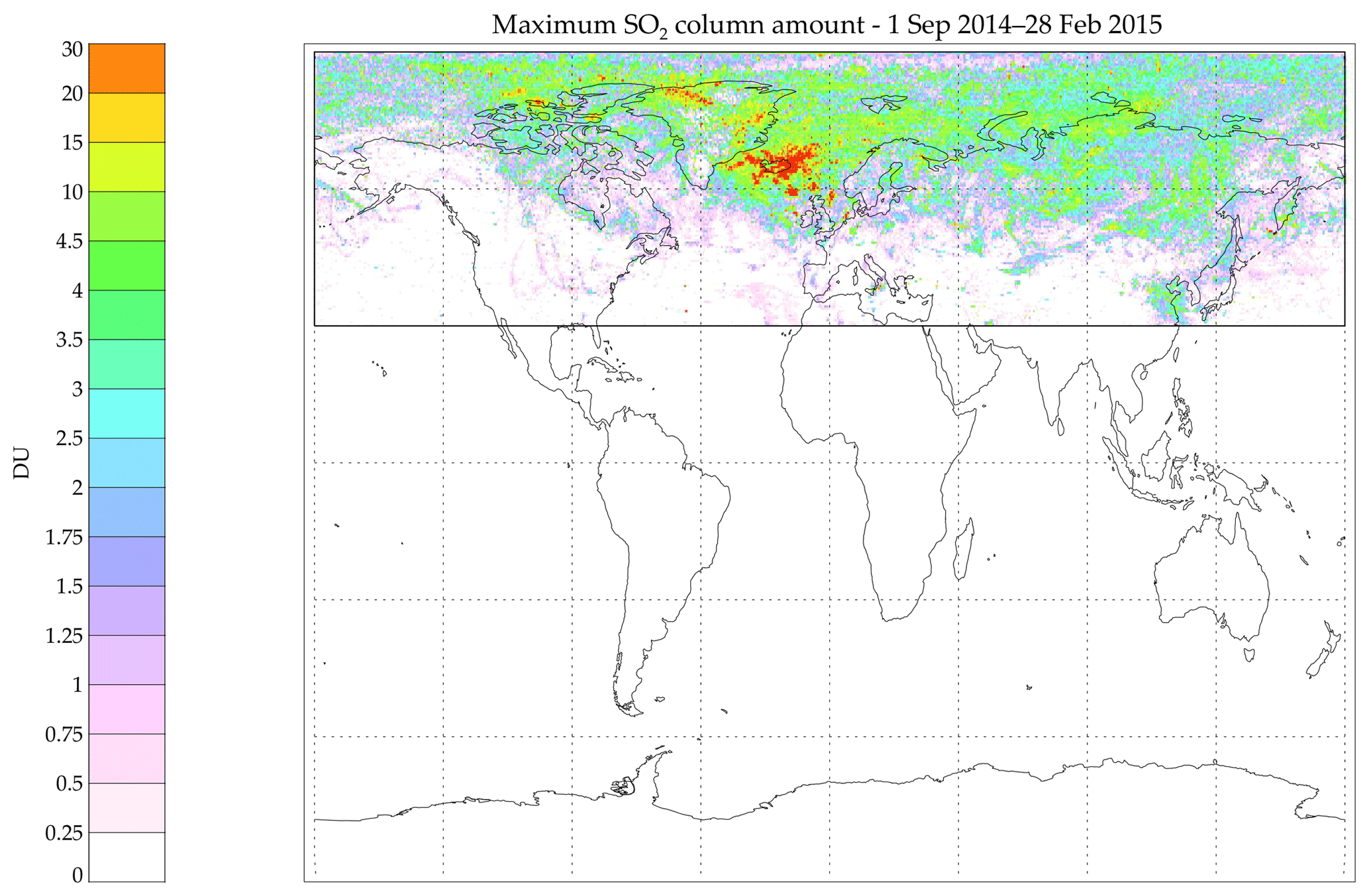
Figure 1Map showing the maximum of the SO2 column amount (in Dobson units, DU) retrieved within the considered area from 30 to 90∘ N (black rectangle) from September 2014 to February 2015.
We perform the iterative retrieval for the pixels that give positive detection results. All the channels in the ranges 1000–1200 and 1300–1410 cm−1 (the 7.3 and 8.7 µm SO2 bands) are simultaneously used in the iterative optimal estimation retrieval scheme to obtain the SO2 amount, the altitude of the plume and the surface temperature. The scheme iteratively fits the forward model (simulations) with the measurements, through the error covariance matrix, to seek a minimum of a cost function. The forward model (FM) is based on RTTOV (Saunders et al., 1999), extended to include SO2 explicitly, and uses ECMWF profiles interpolated to the measurement time and location. The error covariance matrix used is the global error covariance matrix in Carboni et al. (2012). It is defined to represent the effects of atmospheric variability not represented in the FM, as well as instrument noise. This includes the effects of cloud and trace gases which are not explicitly modelled. The matrix is constructed from differences between FM calculations (for clear-sky driven with ECMWF profiles) and actual IASI observations for a wide range of conditions, when we are confident that negligible amounts of SO2 are present. Only quality-controlled pixels are considered: these are values where the minimisation routine converges within 10 iterations, the SO2 amount is positive, the plume pressure is between 0 and 1100 mb and the cost function is less than 10. A comprehensive error budget for every pixel is included in the retrieval. Rigorous error propagation, including the incorporation of FM parameter error, is built into the system, providing quality control and comprehensive error estimates on the retrieval results. The IASI SO2 retrieval is not affected by underlying cloud. If the SO2 is within or below a cloud layer its signal will be masked and the retrieval will underestimate the SO2 amount.
The retrieval results from the Metop-A orbits during the period from September 2014 to February 2015 and from 30 to 90∘ N are combined (twice a day, i.e. morning and afternoon overpasses) to produce maps of retrieved SO2 amount and altitude. The animation in the Supplement (S1) shows the evolution of the plume for each day. The Holuhraun eruption is the main source of SO2 over that period. Other minor sources include SO2 emitted from intermittent volcanic activity on the Kamchatka Peninsula, Etna volcano (28 December 2014, 1, 2 and 21 January 2015) and anthropogenic SO2 emissions from Beijing, China. Satellite observations at the pixel level do not provide sufficient information to distinguish between SO2 from Holuhraun and SO2 from other sources. For example, the elevated SO2 near Beijing on 21 December 2014 appears to be from an anthropogenic source, but the elevated SO2 in the same area on 31 December 2014 is from the Holuhraun eruption. In this study all the SO2 measured from 30 to 90∘ N between September 2014 and February 2015 is referred to as Holuhraun SO2.
Over the course of 6 months the eruption plume dispersed across the Northern Hemisphere. Figure 1 shows the maximum SO2 column amount retrieved during the 6-month period and illustrates that SO2 from the Holuhraun eruption was dispersed over large parts of the Northern Hemisphere, including poleward of the Arctic circle. For the majority of the time, the plume circulated around the pole and the northern regions (see animation in S1), overpassing Scandinavia, eastern Europe, Russia, Greenland and Canada several times. The plume overpassed Europe on multiple occasions, most often northern Europe (Schmidt et al., 2015; Ialongo et al., 2015; Zerefos et al., 2017; Steensen et al., 2016; Twigg et al., 2016; Boichu et al., 2016), but also Italy (22 October 2014) and Spain, and reached as far south as Morocco, Algeria (on 5 and 6 November 2014 respectively) and the Greece–Macedonia–Albania region (5 and 6 January 2015).
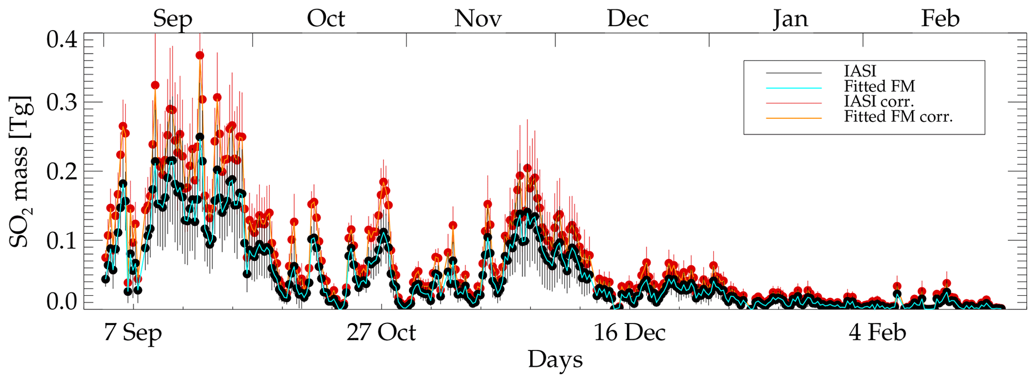
Figure 2Time series of SO2 mass as a function of day from 1 September 2014. The plot shows the IASI mass (obtained from the retrieval) with error bars in black and the fitting of the flux retrieval (Sect. 5) with the cyan line. Red circles and orange line show the masses corrected for cloud presence and their fitting of the retrieval.
IASI orbits are grouped into 12 h intervals in order to have two maps each day of IASI-retrieved SO2 amount and altitude. These maps are gridded onto 0.125∘ latitude and longitude boxes following Carboni et al. (2016). The SO2 mass time series is obtained by summing the mass values of the regularly gridded map for each 12 h period. The same procedure has been used for the errors, this means that the sums of errors of grid boxes are considered as errors on the total masses (this could be an error overestimation but we cannot consider the usual errors in quadrature due to the possible presence of systematic error, e.g. the errors are not independent). The time series of SO2 mass, together with the errors, are presented in Fig. 2. The largest SO2 mass is found in September 2014 (up to 0.25 Tg), when the eruption was most powerful. The SO2 mass decreases during October 2014 (with some peak values around 0.1 Tg), then increases around end of November and beginning of December 2014 (up to 0.15 Tg). The SO2 mass steadily declines during January and February 2015 as the eruption comes to an end. There is no detection of a SO2 plume attached to the vent in the second half of February (and the SO2 mass for this period, reaching a value up to 0.01 Tg, is from a non-Icelandic source).
The SO2 mass present between two altitude levels was estimated using the method by Carboni et al. (2016) to produce the vertical distribution of SO2. In this study the vertical distribution of SO2 was estimated every 12 h from 0 to 10 km with a vertical resolution of 0.5 km for all latitudes north of 30∘ N. Both the young emitted plume, as well as the mature plume that had been transported around in the Northern Hemisphere for a few days, are included in the distribution. The time series of the SO2 vertical distribution for the Holuhraun eruption is shown in Fig. 3. The centre of mass of the plume closest to the vent can be used as a rough estimate for the injection height. Figure 3 shows the time series of two data sets: (i) the vertical distribution and (ii) the altitude of the centre of mass of the SO2 values within 500 km of the vent. The altitude of the centre of mass is less than 4 km for the majority (96 %) of the measurements.
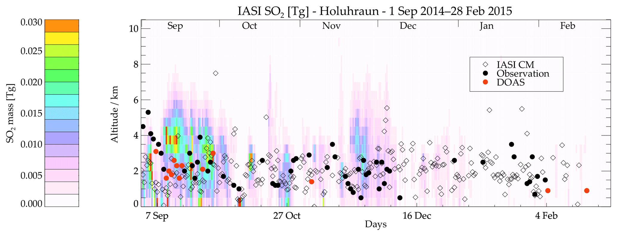
Figure 3SO2 vertical distribution in kilometres above sea level. The colours represents the mass of SO2 and dark red represents values greater than 0.03 Tg. Every column of the plot is generated from an IASI map (one every 12 h; Fig. 1 and Supplement files). The black diamonds show the altitude of the centre of mass (CM) computed with the IASI pixels within 500 km from the vent, and the red and black dots show the DOAS measurements and other observations from Pfeffer et al. (2018).
Part of the SO2 plume can be missed by this IASI scheme, and the derived SO2 masses should be considered as a minimum. The presence of low thermal contrast can prevent the detection of SO2. While cloud below the plume should not be a problem for this scheme, the presence of cloud above the plume will smooth the spectral signature of SO2, causing underestimation of the retrieved SO2 amount (Carboni et al., 2012). At its most extreme this effect can completely erase the SO2 signal (for a cloud layer with zero transmittance).
We estimate the percent of SO2 mass missing due to cloud above the plume as a function of cloud optical depth and altitude above the SO2 plume using the same simulations with a default atmosphere used in Fig. 6 of Carboni et al. (2012). Using the European Space Agency cloud Climate Change Initiative data set (Stengel et al., 2017, ESA cloud CCI) of Advanced Very High Resolution Radiometer – AVHRR (same platform as IASI, i.e. same local overpassing time) L3 monthly mean statistic, we computed the following:
-
Monthly mean histograms of frequency of cloud optical depth at 550 nm, τ, was averaged over the globe. τ is not present in the cloud L3 database for locations without daylight (e.g. visible channels) and most of the Icelandic plume in the winter months is without daylight. As a consequence, here we are assuming the global histogram of frequency of τ is valid over the plume region.
-
Monthly mean histograms of frequency of cloud altitude are averaged over the plume region (30 to 90∘ N). Cloud altitude is available for all locations and during winter months.
We consider the measured mass Mmeas to be the difference between the true mass Mcorr and the missing one Mmiss:
We can rewrite this as follows:
The term within the bracket on the right is the correction factor. We compute the correction factor, C, for every month of the eruption as a function of altitude and apply it to the vertical distribution data set.
with
where Z(h) is the fraction of SO2 “missed” in the measurements due to cloud above the plume. Z(h) is estimated as the product of the probability of having cloud above altitude h, F(h) times the attenuation due to cloud, A.
The probability of having cloud above h has been estimated from the ESA cloud CCI data for the region considered for the volcanic plume (latitude >30∘ N) as the number of cloud retrievals above altitude h divided by number of observations.
Attenuation due to cloud (A) is the sum of the frequency of having a cloud with a cloud optical depth f(τ) times the attenuation due to a cloud with the same optical depth a(τ).
f(τ) has been estimated using the monthly mean histogram of frequency of cloud optical depth, estimated over the globe. a(τ) has been estimated by running the SO2 retrieval using, as IASI measurements, simulated spectra with water cloud above the plume, using the default atmosphere and different optical depths τ. For optical depths bigger than 10 the attenuation is 1 (cloud is opaque and completely masks the SO2 signal). Figure 4 shows the correction factor together with the SO2 vertical distribution obtained from the IASI retrieval and SO2 vertical distribution corrected for underestimation due to cloud cover.
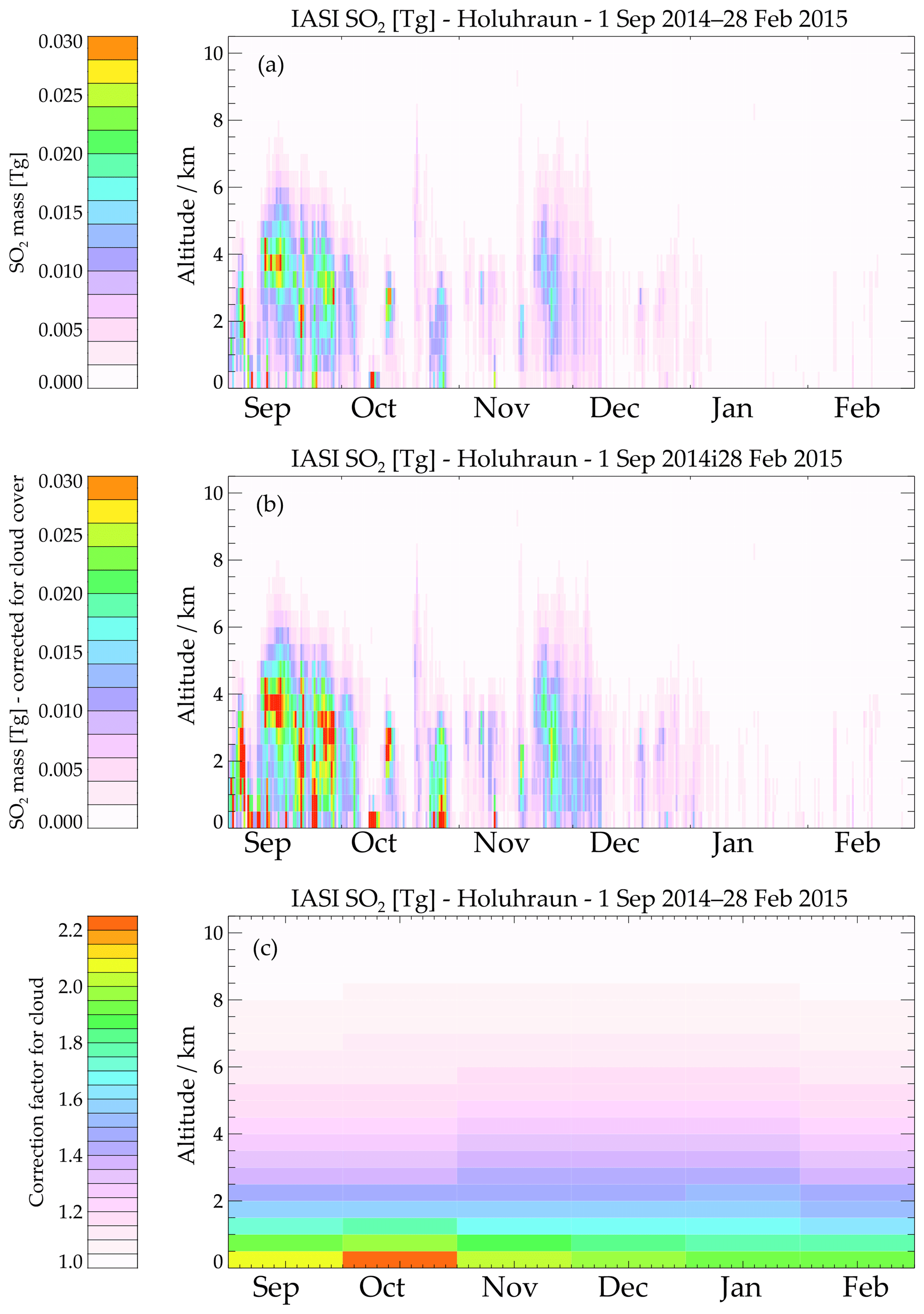
Figure 4SO2 vertical distribution in kilometres above sea level. The colours represent the mass of SO2, and dark red represents values higher than the colour bar. Every column of the plot is generated from an IASI map (one every 12 h). Panel (a) shows the data obtained from the IASI maps. Panel (b) is (a) times the correction factor (to include SO2 that statistically has been missed by the IASI measurements due to cloud above the plume). Panel (c) is the correction factor C(h).
In the following section the emission fluxes have been estimated with both the original SO2 masses (obtained from IASI retrieval scheme explained in Sect. 2) and the masses corrected by cloud cover (this section).
We estimate the missing SO2 mass due to thermal contrast by comparison with OMI SO2 (Theys et al., 2015) for the months of September and October 2014, as the OMI data set does not cover all of the time period of the eruption due to the lack of solar radiance during the winter. We compare, with visual inspection, the daily maps of IASI and OMI and identify the parts of the plume missing from IASI detection (and consequently missing in the IASI retrieval). Table 1 presents the list of all areas identified and the SO2 estimate from OMI (BIRA-IASB algorithm).
Table 1Areas of plume missing from IASI detection scheme and OMI SO2 mass estimate in the area, assuming two different altitudes.
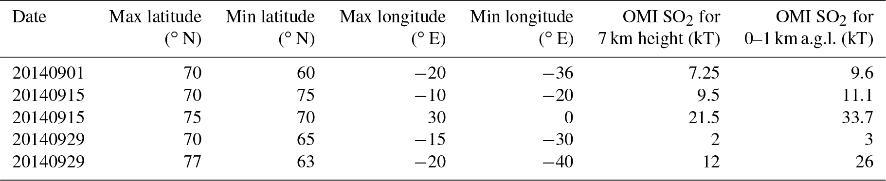
The total mass of SO2 missed due to thermal contrast is estimated to be a few percent of the emission estimate by IASI. In particular, the missing plume for the first 2 months, estimated with OMI 0–1 km, has a total mass of 0.08 Tg of SO2 that corresponds to 3 % percent of the emission estimate by IASI (see Sect. 5 for emission estimate). Cloud could also be a problem for OMI, for such low-altitude SO2, and OMI values could be off by a factor of 2–3, which will change the underestimation to 6 %–9 % (instead of 3 %).
The time series of SO2 fluxes and the coefficient of an average exponential decay of SO2 (the state vector x) are retrieved from the time series of SO2 mass (the measurement vector y) using the optimal estimation scheme of Rodgers (2000). The solution (x, the vector of parameters that we want to retrieve) gives the most probable x given the measurements y and the a priori knowledge xa. The state vector x is found by minimising the cost function:
where F is the forward model (that simulates the measurement given the state vector), xa is the a priori value of the state vector and Se and Sa are the measurement and a priori error covariance matrices. Se and Sa are diagonal matrices with the variances (square of errors) of y and xa respectively as their diagonal elements. The a priori values used were 0.2±0.2 Tg day−1 for flux and 2±2 day for the e-folding time: these values reflect the variability of lifetime found in the literature for low tropospheric emission (Carn et al., 2016; Lee et al., 2011).
To retrieve the time series of SO2 fluxes the state vector x was defined as follows. The first element of the state vector is the average SO2 e-folding time (λ) for the period analysed; the following xi elements are the average emission flux fi between the two IASI estimates of SO2 mass at time ti−1 and ti:
To define the forward model F we consider that the SO2 mass m measured by the satellite is a function of time and that the mass decays proportionally to the mass itself, plus a source term of flux f is added. These terms give a first-order differential equation:
Assuming a constant flux f over the time interval Δt between two consecutive mass estimates mi and mi−1, the solution becomes
where λ (with ) is the average e-folding time. Equation (11) is the forward model F(x).

Figure 5Time series of emission fluxes of SO2. To facilitate the comparison with the flux estimates from Schmidt et al. (2015), (a) presents values (for the first month only) of the retrieved SO2 flux time series from IASI measured mass in black with grey error bars, the retrieved flux time series from corrected IASI mass in red with orange error bars and DOAS ground measurements from Pfeffer et al. (2018) in blue (blue bars show the errors, dotted bars show the maximum and minimum values measured that day). Panel (b) shows the 6-month time series with the same colour coding.
We used optimal estimation (OE) to fit the measured time series of mass loading with a forward model that reproduces the time series as a function of emission fluxes and SO2 e-folding time. This forward model (Eq. 11) is the inverse of Eq. (6) in Theys et al. (2013), section “Delta-M method”. Both equations derive from the solution of the same differential equation (Eq. 10). In Theys et al. (2013) the fluxes are obtained assuming the e-folding time; here, the fluxes and the averaged e-folding time and their uncertainties are estimated simultaneously based on OE.
Figure 2 shows the fitting of the measurements y with the forward model F, while Fig. 5 shows the retrieved fluxes with errors.
The flux time series follows a similar pattern to the SO2 mass time series, with the highest values in September 2014. IASI determined fluxes are provided here with the ground-based measurement fluxes provided in parenthesis (described in Sect. 5). The September daily average was 0.06 Tg day−1 (0.09) and the September daily maximum was 0.26 Tg day−1 on the 20 September (0.19). The October average flux was 0.023 Tg day−1 (0.083), with peak values of 0.15 and 0.12 Tg day−1 on the 11 and 19 October (0.10). The November average flux was 0.029 Tg day−1 (0.069). The flux increases in the second part of November to a maximum of 0.13 Tg day−1 on the 23 November (0.13). The estimates for December, January and February show decreasing fluxes with monthly averages of 0.016, 0.006 and 0.005 Tg day−1 respectively (0.026, 0.028, 0.016). The monthly averages are lower than those measured by the ground-based measurements, while the maximum daily averages for each month are generally higher. The UV ground-based measurements for the dark months of December, January and February are sparse, with only 10 measurements over these 3 months. There was only 1 day with measurements at the beginning of December, then 6 days with measurements in the second half of January and 3 days with measurements in February. The extrapolated flux from the ground-based measurements through December to the first half of January is consistent with the error bars from the IASI estimates. The differences in monthly means between the ground-based measurements and the IASI flux estimates in the sunny months are explainable by low values with large error. The fluxes calculated for September 2014 are consistent with Schmidt et al. (2015) (e.g. up to 0.12 Tg day−1 during early September, 0.02–0.6 Tg day−1 between 6 and 22 September, 0.06–0.12 Tg day−1 until the end of September).
The total mass of SO2 emitted by the eruption is obtained by summing all the fluxes, fi, output by the retrieval and multiplying by the corresponding Δti. The error associated with the total mass emitted is obtained by adding in quadrature the errors δfi multiplied by the time interval Δti. The maximum value of total mass emitted is obtained by summing all the fluxes plus the uncertainty and the minimum value is obtained by summing all the fluxes less the uncertainty (negative values are set to zero). This gives a total mass of emitted SO2 of 4.4±0.8 Tg with a maximum of 11.6 Tg and a minimum of 0.4 Tg. The retrieved averaged e-folding time is 2.4±0.6 days.
Note that, in using an average SO2 e-folding time for the entire eruption period, any variation in e-folding time will be interpreted as an inverse variation in the estimated flux; i.e when the “real” e-folding time is higher than the retrieved one, the flux will be overestimated and vice versa. The flux uncertainties include the errors in flux due to the variation in e-folding time. The SO2 lifetime can vary significantly on a daily basis mainly as a function of water vapour and solar irradiation. Also, note that any e-folding time shorter than the retrieved one can fit the measurements and give higher fluxes. Given these caveats, the value of the e-folding time (2.4±0.6 days) is consistent with the mean lifetime of 2.0 days estimated for September 2014 (Schmidt et al., 2015). Their estimate was based on minimising the difference between the SO2 amount from the NAME dispersion model and the IASI and OMI satellite measurements.
Figure 5 shows that higher values (peaks) of SO2 flux often alternate with lower values (below 0.02 Tg day−1), even during periods that have been identified as generally characterised by higher fluxes. This intermittent flux behaviour has important implications in terms of the estimate of total SO2 emitted.
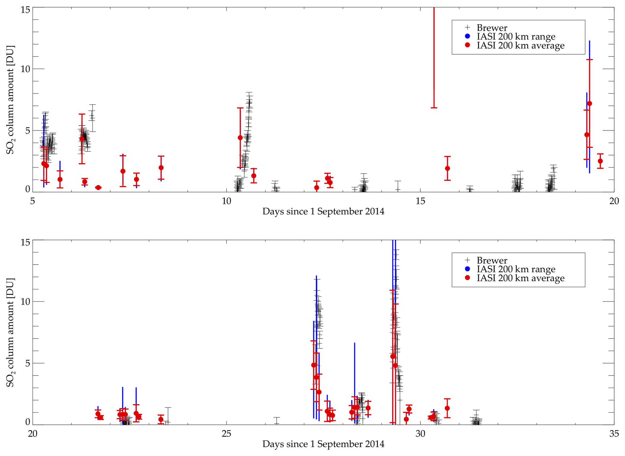
Figure 6Time series of the SO2 column amount (DU) measurements at Sodankylä as a function of day from the 1 September 2014. Black symbols are the Brewer measurements with error bars, red symbols are the mean and standard deviation of all the IASI measurements within 200 km, and blue lines represent the maximum and minimum of the IASI measurements.
Gauthier et al. (2016) used thermal infrared (TIR) data from SEVIRI on board the geostationary satellite Meteosat Second Generation (MSG) to retrieve an SO2 mass time series from 1 September 2014 to 25 November 2014. Their daily retrieved mass values are lower compared to the IASI values reported here due to the smaller geographic area considered and possibly due to the lower sensitivity of SEVIRI. Nevertheless they estimate a total SO2 emitted mass of 8.9±0.3 Tg for the period September 2014 to November 2014, which is a factor of 2 higher than IASI.
Our understanding is that the Gauthier et al. (2016) scheme produced valid measurements when the SO2 loading increased with respect to the previous measurement. This leaves data gaps when the SO2 measured remains constant or decreases. The resulting data gaps were filled by linearly interpolating between two valid measurements. This has a tendency to bias flux estimates in favour of increasing SO2 loading. The data set of Gauthier et al. (2016) contains several days with no valid flux estimates and, for these data gaps, the interpolation of valid measurements into the gaps could account for their discrepancies with our data set. The ground-based measurements reported in Pfeffer et al. (2018) suggest an intermediate value of 7.3 Tg over this time interval.
The conditions of the Holuhraun eruption are significantly different to eruptions investigated in previous studies using IASI (Carboni et al, 2016), because the plume from Holuhraun was confined to altitudes between the surface and 6 km at high-northern latitudes and because the eruption took place during the autumn and winter months. As a result there is less radiance and low (or negative) thermal contrast between the surface and the first layer of the atmosphere. These conditions lead to lower sensitivity for measurements in both the UV and TIR spectral range. Nevertheless, a cross-comparison with other available measurements is informative when assessing our results. The following comparisons are an addition to previous comparisons done between UV satellite measurements and a dispersion model (Schmidt et al., 2015) and balloon measurements (Vignelles et al., 2016).
First the IASI data set is compared with ground-based Brewer measurements of the SO2 column amount of the mature plume over Finland. Successively, the plume height is compared with near-source measurements in Iceland using ground- and aircraft-based visual observations, web camera and NicAIR II infrared images, triangulation of scanning DOAS instruments and the location of SO2 peaks measured by DOAS traverses as reported in Pfeffer et al. (2018).
The Brewer ground measurements (Ialongo et al., 2015) were made at Sodankylä (67.42∘ N, 26.59∘ E). The SO2 column amounts are routinely obtained from the direct solar irradiances at wavelengths of 306.3, 316.8 and 320.1 nm by using the same Brewer algorithm as for the ozone retrieval (Kerr et al., 1988). The method is based on the Lambert–Beer law, which describes the attenuation of the direct solar irradiance reaching the Earth's surface at certain wavelengths due to the atmospheric constituents. In order to avoid the effects of stray light at short wavelengths, the measurements corresponding to large air mass values (after 14:20 UT) are not included. The SO2 column amounts in Sodankylä are typically close to zero with an estimated detection limit of about 1 DU. Ialongo et al. (2015) compared the SO2 column amount values from the Brewer and OMI measurements in Sodankylä during September 2014. The differences between OMI and Brewer retrievals were usually smaller than 2 DU.
The comparison here is performed by averaging all the IASI pixels that pass quality control within 200 km of the ground measurements. The Brewer instrument measures in the UV and thus only in daylight conditions. This means that only the first month of the eruption can be considered. Figure 6 shows the time series of the SO2 column amount from both ground measurements and IASI as a function of time. All the plume episodes (with SO2 amount larger than 2 DU) are consistent between the two data sets with the exception of 15 and 19 September when the plume only passes over the northern part of the 200 km circle in the IASI data and does not pass over the ground measurement station. This means that, while IASI presents high SO2 measurements, elevated values are not observed in the Brewer measurements.
There are a few days of low (less the 2 DU) SO2 reported by only one of the two instruments (IASI or Brewer), meaning that the detection limit of one of the instruments is not exceeded. This is consistent with the IASI minimum error for low-altitude plumes (2 DU for plumes below 2 km, Carboni et al., 2016) and with the Brewer minimum error (2 DU, Sellitto et al., 2017).
The ground-based measurements of the eruption cloud-top height were collected from multiple techniques including ground- and aircraft-based observations, web camera, ScanDOAS, MobileDOAS and NICAIR II IR camera (Pfeffer et al., 2018). The ScanDOAS and MobileDOAS approaches and IASI retrievals, provide the height of the centre of mass of the plume, while the other techniques provide the height of the top of the plume. Figure 3 presents the ground-based and IASI altitudes together. In general, the IASI and ground-based altitudes agree that the altitudes varied mainly between 1 and 3 km; however they do not agree particularly well on any specific day.
The time series of the ground-based (Pfeffer et al., 2018) and IASI flux estimates are presented in Fig. 5. Within error, they generally agree. There are a few significant differences between the two data sets: two values in October–November 2014 and some values at the end of January and February. The ground-based measurements in November alternate between very high and very low values. On 5 November 2014, the ground-based value is significantly higher than the IASI flux estimate for that day. Pfeffer et al. (2018) suggest the high values in November could be due to degassing from a continually replenishing lava lake contributing to the total gas in addition to the degassing from the magma being erupted. The plume altitude was less than 2 km on this day and under these conditions IASI values can be underestimates. The total mass emitted can be estimated using the ground-based measurements as the integral below the red line in Fig. 2 (i.e. interpolating flux values). Even if the majority of fluxes are consistent with each other within the error estimate, the total mass calculated by IASI (4.4 Tg) and IMO (9.6 Tg) differs by a factor of 2. The 5 November discrepancy contributes significantly to this difference.
The first satellite-based SO2 flux data set of the full 2014–2015 Holuhraun eruption has been estimated using the IASI instruments. The data set provides a flux estimate every 12 h for the entire eruption. Thermal infrared spectrometers are the only satellite instruments that could follow the SO2 plume around the Arctic in the absence of solar irradiation during the winter months of the eruption. The low altitude of the SO2 plume and cold underlying surface reduces IASI sensitivity to SO2; however the results compare reasonably well with ground-based near and distal measurements. The observations show that the Holuhraun plume passed over large parts of the Northern Hemisphere during the eruption. The time series of the vertical distribution of SO2 showed a low-altitude plume confined mainly within 0–6 km. The time series of SO2 masses showed a maximum of 0.25 Tg of atmospheric loading in September 2014. A new optimal estimation scheme was developed to calculate daily SO2 fluxes and e-folding time based on satellite-retrieved atmospheric SO2 burdens. Application of the method gave estimates of SO2 flux of up to 200 kt day−1. The minimum total mass of SO2 was calculated to be 4.4±0.8 Tg and the average SO2 e-folding time was found to be 2.4±0.6 days. By comparison with the OMI data set during the summer months of the eruption we estimate that the SO2 masses missed due to low thermal contrast are of the order of a few percent (3 %) of the total emission. We estimated the SO2 mass missed due to cloud above the SO2 plume that is masking the signal, using AVHRR cloud CCI data set monthly mean.
Results show a correction factor increasing with decreasing altitude from one (no underestimation of SO2 masses) at the top of the cloud around 9 km up to a factor of 2 (we measure 50 % of the true mass) for plumes between 0 and 1 km. Applying this correction resulted in a total mass, emitted during the 6 months of the eruption, of 6.7±0.4 Tg and little change in the average e-folding time (2.5±0.7). The IASI flux data reported here are representative of every 12 h and with no data gaps. Other emission estimates include the interpolation (or extrapolation) of fluxes where there are no measured data; this could produce discrepancies between estimates made using different methods.
IASI: Atmospheric sounding level 1C data products are available at https://catalogue.ceda.ac.uk/uuid/ea46600afc4559827f31dbfbb8894c2e (EUMETSAT, 2009). IASI retrieval of sulfur dioxide (SO2) column amounts and altitude data are available at https://catalogue.ceda.ac.uk/uuid/d40bf62899014582a72d24154a94d8e2 (Carboni et al., 2019). ESA Cloud CCI data sets are available at http://www.esa-cloud-cci.org (ESA Cloud CCI project team, 2016). Brewer SO2 ground measurements at Sodankyla are available in the Supplement. Icelandic observation and DOAS measurements are available in Pfeffer et al. (2018).
The supplement related to this article is available online at: https://doi.org/10.5194/acp-19-4851-2019-supplement.
EC developed the retrieval schemes, performed the IASI analysis and drafted the paper. TAM and AS contributed to the analysis and the writing of all the versions of the paper. RGG contributed to developing the retrieval schemes and provided advice and support throughout all the process. MAP provided DOAS measurements, fluxes and altitude observations together with a description of the eruption and discussions of the results. II provided the Brewer ground-based measurements and participated in the discussion of the results. NT provide the OMI data and discussion. All authors contributed toward revising and improving the paper.
The authors declare that they have no conflict of interest.
Elisa Carboni, Roy G. Grainger and Tamsin A. Mather were supported by the NERC Centre for Observation and Modelling of Earthquakes, Volcanoes, and Tectonics (COMET). We thank JASMIN for the fast processing of our retrieval scheme, CEDA and EUMETSAT for IASI level 1 data set, and CEDA and ECMWF for atmospheric profiles. We thank the reviewers for their constructive comments.
This paper was edited by Rainer Volkamer and reviewed by two anonymous referees.
Boichu, M., Chiapello, I., Brogniez, C., Péré, J.-C., Thieuleux, F., Torres, B., Blarel, L., Mortier, A., Podvin, T., Goloub, P., Söhne, N., Clarisse, L., Bauduin, S., Hendrick, F., Theys, N., Van Roozendael, M., and Tanré, D.: Current challenges in modelling far-range air pollution induced by the 2014–2015 Bárðarbunga fissure eruption (Iceland), Atmos. Chem. Phys., 16, 10831–10845, https://doi.org/10.5194/acp-16-10831-2016, 2016. a, b
Carboni, E., Grainger, R., Walker, J., Dudhia, A., and Siddans, R.: A new scheme for sulphur dioxide retrieval from IASI measurements: application to the Eyjafjallajökull eruption of April and May 2010, Atmos. Chem. Phys., 12, 11417–11434, https://doi.org/10.5194/acp-12-11417-2012, 2012. a, b, c, d, e
Carboni, E., Grainger, R. G., Mather, T. A., Pyle, D. M., Thomas, G. E., Siddans, R., Smith, A. J. A., Dudhia, A., Koukouli, M. E., and Balis, D.: The vertical distribution of volcanic SO2 plumes measured by IASI, Atmos. Chem. Phys., 16, 4343–4367, https://doi.org/10.5194/acp-16-4343-2016, 2016. a, b, c
Carboni, E., Taylor, I., and Grainger, D.: IASI retrieval of sulphur dioxide (SO2) column amounts and altitude, 2014-09 to 2015-02, version 1.0, Centre for Environmental Data Analysis, available at: http://catalogue.ceda.ac.uk/uuid/d40bf62899014582a72d24154a94d8e2, last access: 29 March 2019.
Carn, S., Clarisse, L., and Prata, A.: Multi-decadal satellite measurements of global volcanic degassing, J. Volcanol. Geoth. Res., 311, 99–134, https://doi.org/10.1016/j.jvolgeores.2016.01.002, 2016. a
ESA Cloud CCI project team: ESA Cloud Climate Change Initiative (Cloud CCI), available at: http://www.esa-cloud-cci.org/ (last access: 29 March 2019), 2016.
EUMETSAT: IASI: Atmospheric sounding Level 1C data products, NERC Earth Observation Data Centre, available at: http://catalogue.ceda.ac.uk/uuid/ea46600afc4559827f31dbfbb8894c2e (last access: 29 March 2019), 2009.
Gauthier, P.-J., Sigmarsson, O., Gouhier, M., Haddadi, B., and Moune, S.: Elevated gas flux and trace metal degassing from the 2014–2015 fissure eruption at the Bardarbunga volcanic system, Iceland, J. Geophys. Res.-Sol. Ea., 121, 1610–1630, https://doi.org/10.1002/2015JB012111, 2016. a, b, c
Gettelman, A., Shindell, J. D. T., and Lamarque, F.: Impact of aerosol radiative effects on 2000–2010 surface temperatures, Clim. Dynam., 45, 2165–2179, https://doi.org/10.1007/s00382-014-2464-2, 2015. a
Gíslason, S., Stefánsdóttir, G., Pfeffer, M., Barsotti, S., Jóhannsson, T., Galeczka, I., Bali, E., Sigmarsson, O., Stefánsson, A., Keller, N., Sigurdsson, A., Bergsson, B., Galle, B., Jacobo, V., Arellano, S., Aiuppa, A., Jónasdóttir, E., Eiríksdóttir, E., Jakobsson, S., Gudfinnsson, G., Halldórsson, S., Gunnarsson, H., Haddadi, B., Jónsdóttir, I., Thordarson, T., Riishuus, M., Högnadóttir, T., Dürig, T., Pedersen, G., Höskuldsson, A., and Gudmundsson, M.: Environmental pressure from the 2014–15 eruption of Bárðarbunga volcano, Iceland, Geochemical Perspectives Letters, 1, 84–93, https://doi.org/10.7185/geochemlet.1509, 2015. a, b
Ialongo, I., Hakkarainen, J., Kivi, R., Anttila, P., Krotkov, N. A., Yang, K., Li, C., Tukiainen, S., Hassinen, S., and Tamminen, J.: Comparison of operational satellite SO2 products with ground-based observations in northern Finland during the Icelandic Holuhraun fissure eruption, Atmos. Meas. Tech., 8, 2279–2289, https://doi.org/10.5194/amt-8-2279-2015, 2015. a, b, c
Ilyinskaya, E., Schmidt, A., Mather, T. A., Pope, F. D., Witham, C., Baxter, P., Jóhannsson, T., Pfeffer, M., Barsotti, S., Singh, A., Sanderson, P., Bergsson, B., Kilbride, B. M., Donovan, A., Peters, N., Oppenheimer, C., and Edmonds, M.: Understanding the environmental impacts of large fissure eruptions: Aerosol and gas emissions from the 2014–2015 Holuhraun eruption (Iceland), Earth Planet. Sc. Lett., 472, 309–322, https://doi.org/10.1016/j.epsl.2017.05.025, 2017. a
Kerr, J. B., Asbridge, I. A., and Evans, W. F. J.: Intercomparison of total ozone measured by the Brewer and Dobson spectrophotometers at Toronto, J. Geophys. Res.-Atmos., 93, 11129–11140, https://doi.org/10.1029/JD093iD09p11129, 1988. a
Lee, C., Martin, R. V., van Donkelaar, A., Lee, H., Dickerson, R. R., Hains, J. C., Krotkov, N., Richter, A., Vinnikov, K., and Schwab, J. J.: SO2 emissions and lifetimes: Estimates from inverse modeling using in situ and global, space-based (SCIAMACHY and OMI) observations, J. Geophys. Res.-Atmos., 116, D06304, https://doi.org/10.1029/2010JD014758, 2011. a
Malavelle, F. F., Haywood, J. M., Jones, A., Gettelman, A., Clarisse, L., Bauduin, S., Allan, R. P., Karset, I. H. H., Kristjansson, J. E., Oreopoulos, L., Cho, N., Lee, D., Bellouin, N., Boucher, O., Grosvenor, D. P., Carslaw, K. S., Dhomse, S., Mann, G. W., Schmidt, A., Coe, H., Hartley, M. E., Dalvi, M., Hill, A. A., Johnson, B. T., Johnson, C. E., Knight, J. R., O Connor, F. M., Partridge, D. G., Stier, P., Myhre, G., Platnick, S., Stephens, G. L., Takahashi, H., and Thordarson, T.: Strong constraints on aerosol-cloud interactions from volcanic eruptions, Nature, 546, 485–491, https://doi.org/10.1038/nature22974, 2017. a
McCoy, D. T. and Hartmann, D. L.: Observations of a substantial cloud-aerosol indirect effect during the Bardarbunga-Veidivdon fissure eruption in Iceland, Geophys. Res. Lett., 42, 10409–10414, https://doi.org/10.1002/2015GL067070, 2015. a
Pfeffer, M. A., Bergsson, B., Barsotti, S., Stefansdottir, G., Galle, B., Arellano, S., Conde, V., Donovan, A., Ilyinskaya, E., Burton, M., Aiuppa, A., Whitty, R. C. W., Simmons, I. C., Arason, A., Jonasdottir, E. B., Keller, N. S., Yeo, R. F., ArngrAmsson, H., JAhannsson, A., Butwin, M. K., Askew, R. A., Dumont, S., von Lowis, S., Ingvarsson, A., La Spina, A., Thomas, H., Prata, F., Grassa, F., Giudice, G., Stefansson, A., Marzano, F., Montopoli, M., and Mereu, L.: Ground-Based Measurements of the 2014–2015 Holuhraun Volcanic Cloud (Iceland), Geosciences, 8, 29, https://doi.org/10.3390/geosciences8010029, 2018. a, b, c, d, e, f, g, h, i
Rodgers, C. D.: Inverse Methods for Atmospheric Sounding: Theory and Practice, World Scientific, River Edge, N. J., 2000. a
Saunders, R. W., Matricardi, M., and Brunel, P.: An improved fast radiative transfer model for assimilation of satellite radiance observations, Q. J. Roy. Meteor. Soc., 125, 1407–1425, https://doi.org/10.1002/qj.1999.49712555615, 1999. a
Schmidt, A., Carslaw, K. S., Mann, G. W., Rap, A., Pringle, K. J., Spracklen, D. V., Wilson, M., and Forster, P. M.: Importance of tropospheric volcanic aerosol for indirect radiative forcing of climate, Atmos. Chem. Phys., 12, 7321–7339, https://doi.org/10.5194/acp-12-7321-2012, 2012. a
Schmidt, A., Leadbetter, S., Theys, N., Carboni, E., Witham, C. S., Stevenson, J. A., Birch, C. E., Thordarson, T., Turnock, S., Barsotti, S., Delaney, L., Feng, W., Grainger, R. G., Hort, M. C., Höskuldsson, A., Ialongo, I., Ilyinskaya, E., Jóhannsson, T., Kenny, P., Mather, T. A., Richards, N. A. D., and Shepherd, J.: Satellite detection, long-range transport, and air quality impacts of volcanic sulfur dioxide from the 2014–2015 flood lava eruption at Bárdarbunga (Iceland), J. Geophys. Res.-Atmos., 120, 9739–9757, https://doi.org/10.1002/2015JD023638, 2015. a, b, c, d, e
Sellitto, P., Salerno, G., La Spina, A., Caltabiano, T., Terray, L., Gauthier, P.-J., and Briole, P.: A novel methodology to determine volcanic aerosols optical properties in the UV and NIR and Ångström parameters using Sun photometry, J. Geophys. Res.-Atmos., 122, 9803–9815, https://doi.org/10.1002/2017JD026723, 2017. a
Steensen, B. M., Schulz, M., Theys, N., and Fagerli, H.: A model study of the pollution effects of the first 3 months of the Holuhraun volcanic fissure: comparison with observations and air pollution effects, Atmos. Chem. Phys., 16, 9745–9760, https://doi.org/10.5194/acp-16-9745-2016, 2016. a
Stengel, M., Stapelberg, S., Sus, O., Schlundt, C., Poulsen, C., Thomas, G., Christensen, M., Carbajal Henken, C., Preusker, R., Fischer, J., Devasthale, A., Willén, U., Karlsson, K.-G., McGarragh, G. R., Proud, S., Povey, A. C., Grainger, R. G., Meirink, J. F., Feofilov, A., Bennartz, R., Bojanowski, J. S., and Hollmann, R.: Cloud property datasets retrieved from AVHRR, MODIS, AATSR and MERIS in the framework of the Cloud_cci project, Earth Syst. Sci. Data, 9, 881–904, https://doi.org/10.5194/essd-9-881-2017, 2017. a
Theys, N., Campion, R., Clarisse, L., Brenot, H., van Gent, J., Dils, B., Corradini, S., Merucci, L., Coheur, P.-F., Van Roozendael, M., Hurtmans, D., Clerbaux, C., Tait, S., and Ferrucci, F.: Volcanic SO2 fluxes derived from satellite data: a survey using OMI, GOME-2, IASI and MODIS, Atmos. Chem. Phys., 13, 5945–5968, https://doi.org/10.5194/acp-13-5945-2013, 2013. a, b
Theys, N., De Smedt, I., Gent, J., Danckaert, T., Wang, T., Hendrick, F., Stavrakou, T., Bauduin, S., Clarisse, L., Li, C., Krotkov, N., Yu, H., Brenot, H., and Van Roozendael, M.: Sulfur dioxide vertical column DOAS retrievals from the Ozone Monitoring Instrument: Global observations and comparison to ground-based and satellite data, J. Geophys. Res.-Atmos., 120, 2470–2491, https://doi.org/10.1002/2014JD022657, 2015. a
Twigg, M. M., Ilyinskaya, E., Beccaceci, S., Green, D. C., Jones, M. R., Langford, B., Leeson, S. R., Lingard, J. J. N., Pereira, G. M., Carter, H., Poskitt, J., Richter, A., Ritchie, S., Simmons, I., Smith, R. I., Tang, Y. S., Van Dijk, N., Vincent, K., Nemitz, E., Vieno, M., and Braban, C. F.: Impacts of the 2014–2015 Holuhraun eruption on the UK atmosphere, Atmos. Chem. Phys., 16, 11415–11431, https://doi.org/10.5194/acp-16-11415-2016, 2016. a
Vignelles, D., Roberts, T., Carboni, E., Ilyinskaya, E., Pfeffer, M., Waldhauserova, P. D., Schmidt, A., Berthet, G., Jegou, F., Renard, J.-B., Ólafsson, H., Bergsson, B., Yeo, R., Reynisson, N. F., Grainger, R., Galle, B., Conde, V., Arellano, S., Lurton, T., Coute, B., and Duverger, V.: Balloon-borne measurement of the aerosol size distribution from an Icelandic flood basalt eruption, Earth Planet. Sc. Lett., 453, 252–259, https://doi.org/10.1016/j.epsl.2016.08.027, 2016. a, b
Walker, J. C., Dudhia, A., and Carboni, E.: An effective method for the detection of trace species demonstrated using the MetOp Infrared Atmospheric Sounding Interferometer, Atmos. Meas. Tech., 4, 1567–1580, https://doi.org/10.5194/amt-4-1567-2011, 2011. a, b
Walker, J. C., Carboni, E., Dudhia, A., and Grainger, R. G.: Improved detection of sulphur dioxide in volcanic plumes using satellite-based hyperspectral infra-red measurements: application to the Eyjafjallajökull 2010 eruption, J. Geophys. Res., 117, D00U16, https://doi.org/10.1029/2011JD016810, 2012. a
Zerefos, C. S., Eleftheratos, K., Kapsomenakis, J., Solomos, S., Inness, A., Balis, D., Redondas, A., Eskes, H., Allaart, M., Amiridis, V., Dahlback, A., De Bock, V., Diémoz, H., Engelmann, R., Eriksen, P., Fioletov, V., Gröbner, J., Heikkilä, A., Petropavlovskikh, I., Jaroslawski, J., Josefsson, W., Karppinen, T., Köhler, U., Meleti, C., Repapis, C., Rimmer, J., Savinykh, V., Shirotov, V., Siani, A. M., Smedley, A. R. D., Stanek, M., and Stübi, R.: Detecting volcanic sulfur dioxide plumes in the Northern Hemisphere using the Brewer spectrophotometers, other networks, and satellite observations, Atmos. Chem. Phys., 17, 551–574, https://doi.org/10.5194/acp-17-551-2017, 2017. a
- Abstract
- Introduction
- IASI SO2 iterative retrieval scheme
- Temporal evolution of SO2 mass and SO2 vertical distribution
- Quantifying satellite-retrieval underestimation
- Daily SO2 fluxes
- Comparison with ground-based and near-source measurements
- Conclusions
- Data availability
- Author contributions
- Competing interests
- Acknowledgements
- Review statement
- References
- Supplement