the Creative Commons Attribution 4.0 License.
the Creative Commons Attribution 4.0 License.
 | 11 Dec 2019
How should we aggregate data? Methods accounting for the numerical distributions, with an assessment of aerosol optical depth
Kirk D. Knobelspiesse
Many applications of geophysical data – whether from surface observations, satellite retrievals, or model simulations – rely on aggregates produced at coarser spatial (e.g. degrees) and/or temporal (e.g. daily and monthly) resolution than the highest available from the technique. Almost all of these aggregates report the arithmetic mean and standard deviation as summary statistics, which are what data users employ in their analyses. These statistics are most meaningful for normally distributed data; however, for some quantities, such as aerosol optical depth (AOD), it is well-known that distributions are on large scales closer to log-normal, for which a geometric mean and standard deviation would be more appropriate. This study presents a method of assessing whether a given sample of data is more consistent with an underlying normal or log-normal distribution, using the Shapiro–Wilk test, and tests AOD frequency distributions on spatial scales of 1∘ and daily, monthly, and seasonal temporal scales. A broadly consistent picture is observed using Aerosol Robotic Network (AERONET), Multiangle Imaging SpectroRadiometer (MISR), Moderate Resolution Imagining Spectroradiometer (MODIS), and Goddard Earth Observing System Version 5 Nature Run (G5NR) data. These data sets are complementary: AERONET has the highest AOD accuracy but is sparse, and MISR and MODIS represent different satellite retrieval techniques and sampling. As a model simulation, G5NR is spatiotemporally complete. As timescales increase from days to months to seasons, data become increasingly more consistent with log-normal than normal distributions, and the differences between arithmetic- and geometric-mean AOD become larger, with geometric mean becoming systematically smaller. Assuming normality systematically overstates both the typical level of AOD and its variability. There is considerable regional heterogeneity in the results: in low-AOD regions such as the open ocean and mountains, often the AOD difference is small enough (<0.01) to be unimportant for many applications, especially on daily timescales. However, in continental outflow regions and near source regions over land, and on monthly or seasonal timescales, the difference is frequently larger than the Global Climate Observation System (GCOS) goal uncertainty in a climate data record (the larger of 0.03 or 10 %). This is important because it shows that the sensitivity to an averaging method can and often does introduce systematic effects larger than the total goal GCOS uncertainty. Using three well-studied AERONET sites, the magnitude of estimated AOD trends is shown to be sensitive to the choice of arithmetic vs. geometric means, although the signs are consistent. The main recommendations from the study are that (1) the distribution of a geophysical quantity should be analysed in order to assess how best to aggregate it, (2) ideally AOD aggregates such as satellite level 3 products (but also ground-based data and model simulations) should report a geometric-mean or median AOD rather than (or in addition to) arithmetic-mean AOD, and (3) as this is unlikely in the short term due to the computational burden involved, users can calculate geometric-mean monthly aggregates from widely available daily mean data as a stopgap, as daily aggregates are less sensitive to the choice of aggregation scheme than those for monthly or seasonal aggregates. Furthermore, distribution shapes can have implications for the validity of statistical metrics often used for comparison and evaluation of data sets. The methodology is not restricted to AOD and can be applied to other quantities.
- Article
(12470 KB) - Full-text XML
- BibTeX
- EndNote


Geophysical data are obtained from a variety of data sources and model simulations across many disciplines in the Earth sciences. As one example, aerosol optical depth (AOD) is often measured on the ground by Sun photometry (e.g. Giles et al., 2019), retrieved from passive (single- or multispectral, single- or multi-view, and single- or multi-polarisation state) or active (lidar) satellite observations (e.g. Kokhanovsky and de Leeuw, 2009; Lenoble et al., 2013; Dubovik et al., 2019) and simulated by global models (e.g. Kinne et al., 2006). While each sensor or model has its own distinct spatial and temporal sampling characteristics, for applications in many research areas it is common to use aggregates represented by daily to seasonal averages and on length scales of the order of tens of kilometres to several degrees. These are often somewhat coarser than the highest resolution available from a technique. For satellite retrievals, these daily or monthly aggregates are known as level 3 (L3) data. Level 2 (L2) data represent an instantaneous snapshot, often along the orbit track at the native resolution of the sensor (or some multiple of it), and level 1 (L1) data consist of the geolocated satellite measured radiances which are used as inputs to L2 algorithms. Daily L3 data are constructed by aggregating L2 retrievals; monthly L3 data are typically constructed by aggregating daily L3 data, although in some cases they have also been constructed from L2 directly, which gives different results if the contributing days have unequal sampling (Levy et al., 2009).
Reasons for preferring L3-type (i.e. aggregated) data for some applications over L2-type data include the decreased storage and computational overhead, the fact that aggregates are typically reprojected onto a regular grid and so are often more user-friendly, and a desire to have a data set with fewer gaps. Gaps can be caused by unfavourable retrieval conditions; for example, algorithms to retrieve atmospheric aerosol or surface reflective and emissive properties often require cloud-free, snow-free, and daytime scenes. Gaps also arise from the simple fact that surface and satellite observations do not observe every location all the time. Unfortunately, sampling incompleteness adds an additional representativity error in comparisons; in some fields, such as aerosol remote sensing, this can be difficult to quantify and sometimes is non-negligible (Levy et al., 2009; Sayer et al., 2010; Colarco et al., 2014; Geogdzhayev et al., 2014; Schutgens et al., 2017). While global or regional model simulations are typically already on a fixed grid and spatiotemporally complete, the use of daily or monthly model averages likewise has the appeal of lower computational requirements and ease of use, particularly when comparing to an incomplete ground-based or satellite product.
While the principles of uncertainty propagation in remote sensing are well established (Povey and Grainger, 2015; Merchant et al., 2017), until recently comparatively little effort (relative to L1 and L2 development) has been put into determining the most meaningful ways to construct L3 data and assess their uncertainties. This occurs despite the wide use of these data products in research. One notable exception is sea surface temperature, for which comprehensive estimates of multiple components of L3 uncertainties have been developed (Kennedy, 2014; Bulgin et al., 2016a, b). Implicit in the calculation of summary statistics such as mean and standard deviation in a L3-type data set (or model average) is the assumption that the points aggregated belong to some local population such that the calculation of summary statistics is meaningful for describing the state of the Earth. The use of binned data is another option, although analyses using binned aggregates are generally less common than those using averages. One fundamental aspect of this is the question of how to average the data; i.e. which distribution's summary statistics provide the most useful and meaningful metrics to report? No simple distribution is likely to provide a perfect fit to any observational data set, so the relevant problem is in finding an approximate distribution sufficient for a particular application. Choice of mean (and often additionally standard deviation), as is most common in many fields (including AOD), takes as a given that the normal distribution (which is described in terms of these two parameters) is an appropriate distribution to summarise this population. For a given mean and standard deviation σn of AOD, the normal frequency distribution is given by
where N is a normalisation constant (the total number of data points). As this is symmetric about , this mean value is also the distribution's median and mode.
This assumption runs counter to the fact that AOD at a given location tends not to be normally distributed, which has been indicated in the literature for at least 50 years. Writing in terms of aerosol-induced turbidity (directly proportional to AOD), Flowers et al. (1969) presented measurements at 500 nm, collected through the early 1960s using Sun photometers designed by Volz (1959) as part of an observation network of several dozen sites across the United States of America (USA). Note that this was but one of several networks observing atmospheric turbidity (sometimes separating aerosols from other contributions and sometimes not) with various types of instruments through the 20th century. Holben et al. (2001) reviews others, with the earliest being bolometer measurements in Washington, District of Columbia (DC), USA, beginning in 1902 (Roosen et al., 1973). Instrumentation and data processing (e.g. calibration, data collection and reporting, and cloud screening) methods limit the accuracy and use of some of these earlier records; Forgan et al. (1993) provide a thorough discussion. Nevertheless, Flowers et al. (1969) found (their Fig. 4) cumulative distribution functions consistent with log-normal distributions, i.e. normal when the data are represented in log space; analogous to Eq. (1), the log-normal frequency distribution is given by
Here and σl are the geometric mean and geometric standard deviation of AOD, respectively; as for the normal distribution, the geometric-mean value is also its median and mode. A base 10 logarithm is used here for numerical convenience. For easier comparison between the two distribution forms, in this study, (i.e. arithmetic mean) and (i.e. geometric mean) are represented and will be discussed in absolute, rather than logarithmic, units. Note that due to the additive properties of logarithms, is equivalent whether calculated as the geometric mean of τ or the arithmetic mean of log 10τ; i.e.
The geometric standard deviation σl is the standard deviation of log-transformed data (log 10τ). Because of this, unlike arithmetic standard deviation, it is a multiplicative rather than additive factor (Kirkwood, 1979), i.e. the central one standard deviation of the data is encompassed by the range to (multiplicative), implying an asymmetric range when expressed in absolute (non-logarithmic) units, compared to (additive) for an arithmetic mean.
Note that Eq. (2) is often expressed in terms of dN∕dτ rather than dN∕dlog 10τ (i.e. linear rather than logarithmic ordinate). In this case, using the chain rule and properties of logarithms, the relation between the two formulations is given by
where ln (10) denotes the natural logarithm of 10, which is approximately 2.30. Some further relations between normal and log-normal distribution parameters, including transformations between the arithmetic and geometric mean and standard deviation, are given by Table 1 of O'Neill et al. (2000) and omitted here for brevity.
Other studies published around this time (e.g. Ahlquist and Charlson, 1967; Volz, 1970; Volz and Sheehan, 1971; Rangarajan, 1972) reported AOD measurements in other parts of the world. These analyses were more concerned with estimating the value and distribution (which turned out to be close to normal) of its wavelength-dependence, via the Ångström exponent α (Ångström, 1929), than those of AOD. This was of interest both for visibility applications and because α was often used to estimate one of the parameters in the aerosol particle size distribution model of Junge (1955, 1963), which was used widely at the time. Intriguingly, one implication of log-normally distributed AOD is that α should be normally distributed (if the data belong to a single population). This arises from the definition of α,
for AOD (τ) at some wavelength λ, approximated in these studies using bispectral AOD measurements at wavelengths λ1 and λ2. Due (again) to the additive properties of algorithms, α as the log-ratio of two log-normal distributions is equivalent to the difference of two normally distributed random variables (even when they are correlated, as is the case for AOD), which is itself normally distributed. If AOD were normally distributed, then (because it is a positive-definite quantity) in low-AOD conditions, α would exhibit significant skew and possibly multiple modes (in high-AOD conditions, α might appear close to normal but with incorrect kurtosis). Hence, the fact that α distributions presented in some of those studies are close to normality, given the fairly low-AOD conditions, support (although are not alone unambiguous evidence for) log-normally distributed AOD populations. One caveat is that α distributions can exhibit false skew dependent on the magnitude and spectral correlation of the uncertainties in τ(λ) (Wagner and Silva, 2008). Note that Eq. (5) is insensitive to the choice of logarithmic base.
Daily and monthly averages of extinction at multiple locations presented by Roosen et al. (1973) also show skewed distributions associated with log-normality, although frequency distributions are not directly shown. Several years later, Malm et al. (1977) and King et al. (1980) presented spectral AOD measurements from the opposite ends (Page and Tucson, respectively) of Arizona, USA. They realised that it was most appropriate to represent the resulting frequency distributions with logarithmic (geometric), rather than arithmetic, averages and standard deviations. More recent work has taken advantage of the great increase in data quality, volume, and coverage possible from better instrumentation and computational power. O'Neill et al. (2000) showed that AOD derived from Sun photometer measurements at a variety of individual Aerosol Robotic Network (AERONET) sites spread around the world tends to have frequency distributions which statistically resemble a log-normal distribution to a much stronger degree than normal. All these previous studies were of data aggregated over time summarised at individual locations; around the same time, providing an early satellite example, Ignatov and Stowe (2000) found approximately log-normal AOD (and normal α) in aerosol retrievals over ocean scenes. This indicated that log-normal tendencies might be found in AOD data also aggregated spatially as opposed to just temporally. Similar skewed distributions were reported by Smirnov et al. (2011) for ship-based Sun photometer AOD observations taken on cruises. Maps of retrieved or simulated AOD, and scatter density plots in satellite validation studies, show a similar pattern (e.g. Kinne et al., 2006; Remer et al., 2008; Sayer et al., 2012): a large cluster of points at a comparatively low AOD, with a rapidly decreasing number of points as AOD increases, corresponding to locations and times affected by severe smoke, dust storms, or pollution episodes.
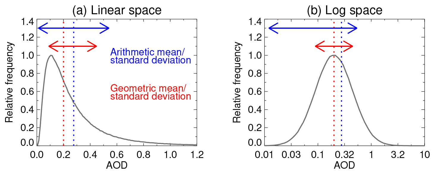
Figure 1Synthetic frequency distributions for log-normally distributed AOD with a mean of 0.2 and geometric standard deviation 0.35, ℒ(0.2,0.352), shown on (a) linear and (b) logarithmic AOD axes. Vertical red and blue dashed lines represent geometric- and arithmetic-mean values, respectively. Horizontal red and blue arrows indicate the range of geometric and arithmetic mean ± one standard deviation.
Due to this asymmetry, normal statistics (i.e. arithmetic mean and standard deviation σn) will overstate the typical level of AOD observed and its variability, implying in some cases unphysical negative AOD. Here “typical” is used in the sense of “common”; the positive tail of log-normally distributed data means that its arithmetic mean lies above its median such that the arithmetic mean is “uncommon” in the sense of being somewhat larger than the median value. This is illustrated in Fig. 1, which compares arithmetic and geometric statistics for a synthetic AOD distribution ℒ(0.2,0.352) similar to that of many locations across the United States and Europe (e.g. O'Neill et al., 2000). The central one standard deviation (1σ) about the mean, which corresponds to an AOD range of 0.09–0.45 (i.e. in log space) when calculated using the geometric mean and standard deviation, correctly encompasses approximately 68.4 % of the data. In contrast calculating arithmetic mean and standard deviation gives 0.28 (i.e. overstating the typical AOD) and 0.27; the resulting 1σ range (, 0.01–0.55) includes 89.2 % of the data (i.e. overstating the variability). Figure 1b reveals the symmetry of the distribution when shown in log space. Thus, representing a log-normally distributed quantity using normal-distribution-appropriate statistics has systematic quantitative implications for the interpretation of the data.
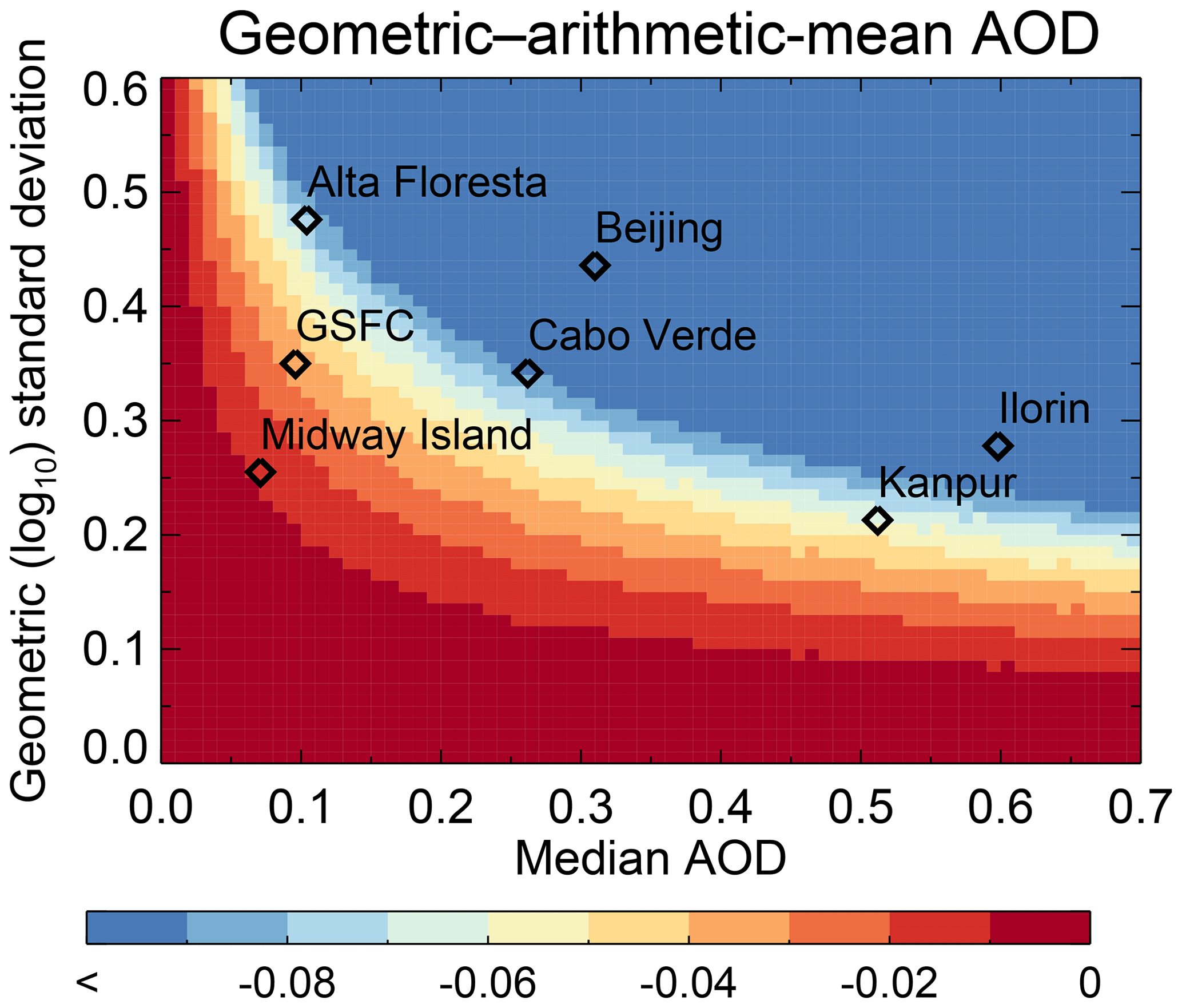
Figure 2Difference between geometric- and arithmetic-mean AOD () as a function of median (equivalent to geometric mean) AOD and geometric standard deviation for log-normally distributed data. Diamonds indicate the median AOD and geometric standard deviation (calculated over all direct Sun data) found at assorted AERONET sites which have been well-used in the literature.
Figure 2 takes a more general look at the difference between geometric- and arithmetic-mean AOD calculated from an underlying log-normal distribution; this becomes more negative as either the median AOD or geometric standard deviation increases (i.e. as the distribution moves rightward or broadens). Also shown are long-term values of both parameters for selected AERONET sites which are frequently used in the literature. The resulting geometric–arithmetic-mean AOD difference for these sites spans from around −0.01 to more negative than −0.10, which are non-negligible values. This implies that, at least on multi-year timescales, knowledge of the shape of the underlying distribution can be important for the choice and interpretation of summary metrics.
Log-normal distributions are common across quantities in the natural sciences and tend to arise when the underlying phenomenon is governed partly by multiplicative (rather than additive) factors; Limpert et al. (2001) provides general examples and discussion. Hinds (1999) and Anderson et al. (2003) discuss aerosol-specific factors such as, for example, changes in emissions or removal (e.g. onset of fires and soil fragmentation on the one hand or precipitation on the other) or turbulence and dispersion affecting different parts of the size distribution, which are not additive in effect. Aerosol particle size distributions may be represented sufficiently well by combinations of log-normal modes (Dubovik et al., 2002); this is common practice in satellite retrieval algorithms. Note that, for a given size distribution, AOD is proportional to total mass. Kok (2011a, b) presented a theoretical model of dust emissions based on fragmentation theory and log-normal size distributions, which agreed with measurements better than existing parametrisations in global models. A further issue important to consider is that the observed distribution of a quantity is a convolution of the true distribution; the sampling of the sensor (or model); and any measurement, model, or retrieval error. Depending on the form of these errors, the underlying shape of a distribution might be skewed. For example if a satellite AOD retrieval algorithm makes a biased assumption about the aerosol single-scattering albedo (SSA), it can lead to a fractional error in retrieved AOD (e.g. Eck et al., 2013), broadening or narrowing the tail of the observed AOD distribution (dependent on whether SSA is under- or overestimated).
Similar behaviour is found for many other remotely sensed quantities; for example, Campbell (1995) assessed log-normality on large scales for oceanic chlorophyll, water-leaving radiance, and photosynthetic yield, while cloud optical depth (COD) is also known to be distributed approximately log-normally (King et al., 2013), and some of the most widely used cloud classification schemes (introduced by Rossow and Schiffer, 1999) are based on joint histograms of (roughly log-normal) COD against cloud-top pressure. Both rainfall rates and cloud particle size distributions can sometimes be represented well by both log-normal and gamma distributions (Cho et al., 2004; Platnick et al., 2017). A commonality these quantities share with AOD is that they are positive-definite quantities (i.e. cannot take zero or negative values) and often have a long tail, which are also features of log-normal and gamma distributions.
Recent efforts by other researchers have helped with understanding spatial and temporal scales in AOD variations and their potential effects on data aggregates. Anderson et al. (2003) used surface-level aerosol scattering and column AOD and found that autocorrelation could remain high on scales of tens to several hundreds of kilometres and timescales of days to weeks. Noting that study, Kovacs (2006) assessed validation statistics of Moderate Resolution Imaging Spectroradiometer (MODIS) AOD against AERONET as a function of the distance of satellite retrievals from AERONET sites. The level of agreement showed site-specific drop-offs with distance, with generally less variability over ocean sites which were less likely to be influenced by local sources. Alexandrov et al. (2004) used a network of shadow-band radiometers across the southern Great Plains in the USA to perform an energy spectrum analysis on AOD variations. They observed a scale break at length scales of around 12–15 km (interestingly, slightly larger than many space-borne L2 AOD products), below which the structure function of AOD variations showed one exponent and above which they showed another, corresponding to regimes where variations were dominated by 3-D and 2-D turbulence, respectively. Using field campaign observations and satellite retrievals over the southeastern USA, Kaku et al. (2018) note that correlation lengths can differ for surface level vs. column aerosol loading. These studies of correlation structure are important for defining suitable scales for a population to be aggregated and for describing how the error characteristics of such aggregates might vary spatially and temporally.
Several studies have sought to assess representation uncertainty in L3-type aggregates; Sayer et al. (2010) examined how the completeness of sampling of satellite AOD retrievals within model grid cells affected the level of agreement between data sets. Li et al. (2016) assessed how representative long-term AERONET sites are on satellite L3 spatial scales and monthly timescales, as part of a larger body of work to characterise and reduce the uncertainty in multi-sensor monthly mean AOD records. From a perspective of comparing global model grid cells to point measurements, Schutgens et al. (2016a) assessed the extent to which representativeness errors caused by coarse model grid size could be decreased by temporal averaging. They found that AOD uncertainties could be decreased to a greater extent than other aerosol properties but that such errors were often still larger than desirable. Schutgens et al. (2017) then attempted to estimate representation uncertainties on ground- or satellite-type aerosol data aggregates on different spatiotemporal scales. They found that spatiotemporal collocation was important, and, as in the prior study, representation errors could still be significant in some cases, such as when near aerosol point sources or in complex terrain. Alexandrov et al. (2016) proposed describing the logarithm of AOD in terms of Gaussian structure functions (accounting for aerosol loading, variance, and autocorrelation) and presented a comparison between MODIS retrievals with global-circulation-model simulations represented in this way. Povey and Grainger (2019) aggregated satellite AOD retrievals on a monthly basis (i.e. L2 to monthly L3 directly) and represented the results in terms of sums of log-normal modes. They found that doing so both highlighted regions of significant variability and aided in identifying systematic differences between data sets.
This analysis aims to complement these other recent studies, building most directly on O'Neill et al. (2000), as a further step towards a more robust calculation and use of AOD aggregates in ground-based, satellite, and model-simulation studies. While the example application is to AOD, the framework introduced is applicable more generally to other (geophysical or not) data aggregates. The central questions to be addressed are as follows: on commonly used spatial and temporal scales, does a normal or log-normal distribution better represent AOD frequency distributions? When and where does the choice matter? When and where might neither distribution be adequate? And what are the implications for L3 data and related analyses if a log-normal representation is used instead? Section 2 describes the data and methodology employed. Section 3 presents the results of the analysis, and Sect. 4 discusses the implications of the findings for the creation and use of aggregated AOD data or model simulations.
2.1 Data and model simulations used
This analysis uses ground-based observations from AERONET, together with satellite retrievals from the Multiangle Imaging SpectroRadiometer (MISR) and MODIS instruments, and model simulations from the Goddard Earth Observing System (GEOS) Version 5 Nature Run (G5NR). All of these have different spatiotemporal sampling techniques and associated uncertainties in their estimates of AOD. Considering a diverse set of data sources such as this provides a more comprehensive picture of the frequency distributions of AOD than would be obtained from only a single data type. It allows the strengths of individual techniques to be used while helping to avoid erroneous conclusions stemming from limitations of individual techniques. The data sources are described below.
2.1.1 AERONET
AERONET provides aerosol (and water vapour) data from Sun photometer measurements, obtained with standardised acquisition, calibration, and processing protocols. This analysis uses the latest Version 3 direct-Sun level 2 (cloud-screened, post-deployment-calibrated, and quality-assured) AERONET AOD data. Note that “level 2” in AERONET terminology refers to quality-assurance level, regardless of temporal aggregation level, as opposed to the satellite level 2, which refers to instantaneous data only. Version 3 includes improvements to sensor characterisation, site geolocation accuracy, and cloud–aerosol discrimination (Giles et al., 2019), particularly in the detection of stable optically thin cirrus cloud layers and rapidly evolving fine-mode aerosol plumes. Here, all direct-Sun observations from all sites (1185 at the time of writing) from the start of 1993 to the end of 2018 are used. Measurement cadence depends on the instrument model used and can be adjusted depending on the desired mix of scan types, but for direct-Sun observations, it is typically every 5–15 min in cloud-free skies during daylight hours.
All instruments deployed as part of AERONET provide AOD at 440, 675, 870, and 1020 nm at a minimum; the majority include additional channels between 340 and 1600 nm, with 500 nm being a common addition. In this analysis, AERONET AOD is interpolated spectrally to 550 nm, as this is a common reference wavelength for many satellite data products and model simulations, although the conclusions do not change if other wavelengths are used instead. Hereafter, mentions of AOD without a specified wavelength refer to AOD at 550 nm. This is performed with a least-squares fit of all available AERONET AODs within the 440–870 nm wavelength range (typically four, more for some configurations) to a quadratic polynomial,
where coefficients a0, a1, and a2 are calculated on a point-by-point basis. This quadratic formulation is more robust to calibration problems in individual channels than a linear two-channel interpolation. It also reflects the fact that the relationship between log (τ) and log (λ) is not linear but shows curvature dependent on fine-mode particle size (Eck et al., 1999; Schuster et al., 2006). When more than two wavelengths are available, this is a more realistic description of the spectral derivative of AOD than the bispectral approximation in Eq. (5). The uncertainty in AERONET midvisible AOD is ∼0.01 (Eck et al., 1999), which is somewhat smaller than typical uncertainties in satellite retrievals or model simulations.
2.1.2 MISR
The latest version, 23, of MISR L2 data provides AOD at 558 nm, over land and ocean, with a horizontal pixel size of 4.4 km; the use of 558 rather than 550 nm has a negligible impact on the analysis here. The instrument includes nine cameras with a maximum swath width around 400 km, although the edges of the scan are not covered by all cameras and so retrievals are provided over a slightly narrower swath. This provides repeat views of a given scene roughly once per week at tropical latitudes and once every 3 d at high latitudes. MISR flies on the Sun-synchronous Terra platform, providing data from early 2000, with a 10:30 local solar equatorial crossing time. Separate processing algorithms are applied over land and dark water; version 23 updates and initial evaluation are provided by Garay et al. (2017) and Witek et al. (2018). These have not yet been validated on a global basis but are expected to reduce some high biases seen over low-AOD water scenes, and low biases seen over high-AOD scenes, reported in validation analyses of previous data versions (e.g. Kahn et al., 2010).
This analysis uses 5 years (2004–2008) of L2 data, corresponding to around half a million retrievals per day (after accounting for unfavourable retrieval conditions). The choice of record length is a balance between the robustness of the analyses and storage and processing concerns; 1 year of the MISR L2 product (MIL2ASAE) corresponds to approximately 170 GB. As an order-of-magnitude estimate, assuming (on average) a revisit time of 5 d and half the data being unsuitable for retrieval due to, for example, cloudiness, approximately 200 views of a given point on the Earth would be expected over a 5-year period. While this would show considerable spatial variation, qualitatively it is expected to be sufficient, as it is well-known from observations and modelling that the main features of the global aerosol system are systematic and repeat year-to-year (e.g. d'Almeida et al., 1991; Holben et al., 2001; Kinne et al., 2006; Remer et al., 2008). Recently, Lee et al. (2018) used MISR (version 22) and MODIS retrievals to assess how many years of data were required (on both an annual and a seasonal basis) for a calculated climatology to converge to within an AOD of ±0.01. They found that over much of the open ocean and many land regions, 5 or fewer years were sufficient, although for some aerosol source regions even the full MISR record (17 years at the time) was insufficient. This does not directly answer the question of the record length that is necessary for the present analysis, although it does suggest that except for near strong source regions the results should sample sufficient interannual variability to be only weakly sensitive to the specific time period chosen.
2.1.3 MODIS
The MODIS instruments fly on the Terra and Aqua platforms; L2 data from the latest Collection 6.1 (C61) from Aqua (launched 2002) are used here for the same 5-year period as the MISR analysis. MODIS Aqua is thought to have slightly better radiometric performance than Terra (e.g. Lyapustin et al., 2014). Additionally, the Aqua orbit has a 13:30 local solar equatorial crossing time, so this provides a higher degree of sampling independence from the MISR retrievals than if MODIS Terra were used. The MODIS Atmosphere aerosol product used here (MYD04) includes retrievals from two Dark Target (DT) algorithms, for pixels identified as water and vegetated land, plus the Deep Blue (DB) algorithm. The C61 DT land algorithm is similar to that of the previous Collection 6 (C6; Levy et al., 2013) but implements an updated surface reflectance model, detailed in Gupta et al. (2016), to reduce a systematic positive bias of DT over urban surfaces. The C61 DB data include numerous small updates to surface and aerosol models and cloud and quality assurance (QA) tests to reduce known error sources (Hsu et al., 2019; Sayer et al., 2019). All three algorithms also benefit from sensor calibration updates. Since C6, MODIS retrievals have included a QA-filtered merged data set combining DB and DT retrievals to increase spatial coverage. The C6 merging algorithm is described by Sayer et al. (2014) and essentially uses the water DT algorithm for water scenes and picks from or averages the DB and DT algorithms dependent on surface type over land. The same merging logic is applied in the creation of the C61 merged product, which is used here. Note that the DT land algorithm permits retrieval of AOD down to −0.05, although negative AOD is unphysical; here, zero or negative AOD values are set to 0.0001 instead (as logarithms are only defined for positive values). The results of this analysis are negligibly sensitive to the choice of AOD floor threshold.
MODIS' 2330 km swath results in near-global daily observations in the tropics and once-daily or twice-daily observations at higher latitudes. Retrievals are provided at the 10 km nominal horizontal pixel size at the sub-satellite point. Towards the edge of the scan, the scan geometries and Earth's curvature cause a “bow-tie distortion” where pixels become larger and consecutive scans begin to overlap (Xiong et al., 2006). This distortion at the edge of the swath is about a factor of 2 in the along-track and 5 in the across-track direction (i.e. 10-fold increase in pixel area), and overlap is close to 100 %, which has consequences for AOD retrieval characteristics (Sayer et al., 2015). For about half of the swath, however, the areal expansion is less than a factor of 2 compared to the nominal 10 km × 10 km pixel size.
2.1.4 GEOS-5 Nature Run
The G5NR is a global 7 km non-hydrostatic mesoscale simulation based on the Ganymed version of GEOS-5 (Putman et al., 2014). The aerosol component is described and evaluated by Castellanos et al. (2018). This is a 2-year (May 2005–2007) simulation, and while some factors (e.g. volcanic and biomass-burning emission sources) were prescribed, meteorology was not. Hence, the G5NR is not a direct simulation of that specific historical period (and should not be compared one-to-one against real observations from that period) but is designed to provide a realistic and representative simulation of the Earth system from which synthetic observations could be generated for, for example, observation system development.
Aerosol output fields are provided on a 30 min time step on a 0.0625∘ regular latitude–longitude grid. This includes column AOD contributed by organic carbon, black carbon, dust, sea salt, and sulfate, and following the recommendations of Castellanos et al. (2018), scaling factors (their Table 3) are applied to these component AODs before summing to get the total AOD. These scaling factors bring the G5NR component AODs into line with a climatology from the Modern Era Retrospective analysis for Research and Applications Aerosol Reanalysis (MERRAero). MERRAero was a long-term reanalysis which assimilated MODIS-based AOD; its aerosol component is evaluated by, for example, Buchard et al. (2015). Data from the simulated year 2006 only are used; Castellanos et al. (2018) noted that G5NR aerosol fields were initialised to zero and so did not use the initial 6 months of the simulation to ensure that equilibrium had been reached. The final 6 months of the simulation are also discarded here to ensure that each calendar month has equal representation in the analysis. As this leaves only four available seasons, G5NR output is analysed on only a daily and monthly basis.
2.2 The Shapiro–Wilk test and its application
Shapiro and Wilk (1965) present a method for testing whether a sample of data is consistent with draws from a normally distributed population. Their derivation included some empirical comparisons to other tests, and they found it to have some advantages over those techniques. Yap and Sim (2011) performed Monte Carlo simulations of various distributions to assess eight different normality tests and found that the Shapiro–Wilk (SW) test has the greatest statistical power in most circumstances. The SW test computes the squared discrepancy between the quantiles of the sample with those expected from random samples from a normally distributed population. Implementations are available in many software packages and languages. The test statistic W for a sample x is defined as
where x(i) indicates the ith smallest sample member (known as the ith order statistic of x), and ai values are weighting coefficients calculated from the expected values (m) and covariance (V) of order statistics from normally distributed data:
The test requires N≥3, and W can take values between 0 and 1. Sarhan and Greenberg (1956) (their Table 1), later corrected in Sarhan and Greenberg (1969), provide V for N≤20; Shapiro and Wilk (1965) provide approximate calculations for larger sample sizes, and Royston (1982, 1992) provide approximate m and V up to N=5000. Relevant sample sizes in the present study are up to several hundred points. As the normal distribution is symmetrical about its mean, the coefficients ai are symmetrical; e.g. for N=6. The coefficients are larger for the outer elements of ai, corresponding to the tails of the data sample (i.e. the outer order statistics x(i)). The numerator of Eq. (7) thus represents a tail-weighted squared sum, while the denominator represents a sum of squared deviations from the sample mean . For normally distributed samples these increase around the same rate such that W is close to 1; for non-normal data the denominator increases more rapidly such that W becomes closer to 0.
Royston (1992) provides a normalisation for W in order to estimate a p value for the result, i.e. the probability that a W score at least as extreme would be observed under the null hypothesis of the sample being drawn from a normally distributed population. The Royston (1992) extension for large N and normalisation are used here. Note that the equivalent test for log-normality is simply W calculated using the logarithm of the data, i.e. here log 10τ rather than τ. A high p value indicates consistency with draws from a normal (or log-normal) distribution. One important point to note is that this test only evaluates the degree of departure from normality: it does not test the importance of that departure. As with any test like this, the power (i.e. efficacy at detecting a given departure) is a function of sample size. Thus for large sample sizes it is easier to detect a discrepancy from normally distributed data even if the discrepancy is trivial. Both of these points should be kept in mind when interpreting the results.
The SW test is employed here as follows. First, spatial distributions of AOD are assessed by aggregating the MISR, MODIS, and G5NR data from their native spatial resolutions to 1∘ (as this is a common spatial scale for L3 AOD products and model output) and applying the SW test without any aggregation in time. The resulting aggregates thus have a daily time step for MISR and MODIS (considering all orbits from a given calendar day) and 30 min for G5NR. Next, temporal variations in AOD within a day are assessed by aggregating the AERONET and (previously spatially aggregated) G5NR data on a daily basis and applying the SW test to each site and grid cell. Aggregating G5NR first in space and then in time is more similar to the way polar-orbiting L3 aggregates sample the global aerosol system (as each L2 product is essentially a near-instantaneous snapshot), although the results are not significantly different if G5NR is analysed first in time and then in space. Finally, the resulting daily aggregates from all data sets are aggregated to monthly and seasonal time steps and the SW test applied to each site and grid cell. Seasons are defined as December–January–February (DJF), March–April–May (MAM), June–July–August (JJA), and September–October–November (SON). Note that the monthly and seasonal calculations use daily as a basis, although results differ negligibly if is used instead.
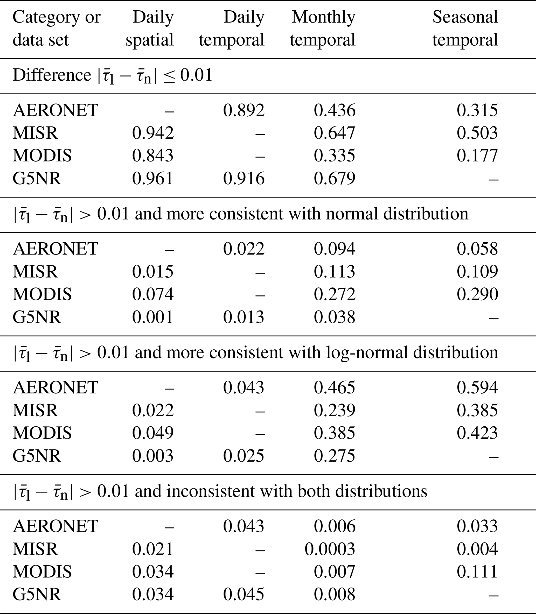
In each case, at least three data points are required for an aggregate to be considered valid; this is the minimum required for the SW test calculation and also the minimum number of observations for AERONET or MODIS standard processing to report a daily average value and the minimum number of days for MODIS products to report a monthly average value. The SW p value is computed for distributions of τ and log 10τ, with resulting p values denoted by p(τ) and p(log 10τ), respectively, and the results fall into one of four possible categories.
-
. In this case the choice of normal or log-normal summary statistics may be considered unimportant, as the resulting arithmetic and geometric averages are similar. The threshold τt is taken as 0.01, which is the typical uncertainty in AERONET midvisible AOD (Eck et al., 1999), and thus represents a reasonable lower bound on achievable uncertainty in average AOD from models and observations at the present time. It is also similar to the thresholds for AOD accuracy over land (±0.016) and ocean (±0.011) estimated by Chylek et al. (2003) to be necessary to be able to constrain the aerosol direct radiative effect to ±0.5 W m−2.
-
, but both p(τ)<pt and p(log 10τ)<pt. In this case both tests return a smaller p value than some threshold pt, indicating evidence of detectable deviation from both normal and log-normal distributions at this significance level. Here pt is taken as 0.001; if the underlying AOD data really were perfectly normally or log-normally distributed (and if the distinction were important), then approximately 0.1 % of data would be expected to fall into this category. However, in reality it is expected that the true distributions are neither of these, and additionally measurement and model errors may distort the observed distributions, leading to more points within this category. Since the p value is not informative about the magnitude of a deviation from normality or log-normality, the additional criterion is included, as it indicates that the magnitude of the AOD difference is large enough that it might be important for some scientific applications (i.e. both statistically and scientifically relevant). Note that the analysis here is only weakly sensitive to the choice of pt.
-
p(τ)>p(log 10τ), p(τ)>pt, and . Here the data are more consistent with draws from a normal than a log-normal distribution, the data are reasonably consistent with a normal distribution, and the difference between arithmetic- and geometric-mean AOD is non-negligible. In this case, the use of normal summary statistics is more appropriate.
-
p(τ)<p(log 10τ), p(log 10τ)>pt, and . The converse of category 3, here the data are best represented by log-normal summary statistics.
The results will be interpreted in terms of relative frequencies of these four categories, as it is important to realise that the idiosyncrasies in real-world data complicate the estimation and calculation of p values. For example, the ideal case of independent random samples from the true population cannot be achieved due to correlated errors in observations or simulations and non-random sampling in space and/or time. SW (or other tests) cannot say whether or not the data are normally or log-normally distributed for any given instance but instead only help say the extent to which the two distributions are reasonable, useful approximations on the whole. In cases of small sample sizes the statistical power of the test may remain small; if the test results for a given area are essentially noise, then similar frequencies of normality and log-normality might be expected. The best that can be done is to keep in mind the limitations of the data, and the statistical tests, in the interpretation of the analysis.

Figure 3Fraction of data falling into each of the four categories of Shapiro–Wilk test results for AOD distributions aggregated temporally over a day. Columns show (left) AERONET and (right) G5NR data (note that the latter were previously spatially aggregated to 1∘). From top to bottom, rows indicate the fraction where the data are more consistent with a normal distribution and , fraction more consistent with a log-normal distribution and , fraction where , and fraction where , and the data show large discrepancies from frequencies expected by both normal and log-normal distributions. For AERONET, at least 50 d are required for a site to be considered valid.
Table 1Mean fraction of data falling into the four categories of SW test results.
3.1 Spatial and temporal variation within a day
Figures 3 and 4 respectively show the categorisation results for temporal (from AERONET and G5NR) and spatial (from MISR, MODIS, and G5NR) frequency distributions of AOD on daily scales. As a summary, Table 1 shows the global mean fractions of data in each category; note that these are the mean of each valid AERONET site and grid cell (i.e. all sufficiently sampled areas are treated equally). Sites and grid cells require at least 50 valid days with data to be included in these statistics. As the spatial sampling between the data sets is quite different (Figs. 3 and 4), the results from the different data sets are not expected to match, but reading the table from left to right gives a sense for how the categorisations change on the different scales assessed. The following general conclusions can be drawn about variability relevant to daily aggregation.
-
Patterns shown between Figs. 3 and 4 are similar; i.e. daily AOD frequency distributions tend to have similar shapes whether for temporal aggregation over a day (as from AERONET or model output) or spatial aggregation on scales of 1∘ (as from polar-orbiting satellites). This establishes that it is reasonable to aggregate spatial and temporal data on a daily basis in a similar way.
-
In areas of low to moderate AOD, including the global oceans, mountains, and fairly clean continental regions, for a strong majority (typically 80 % or more) of days the difference between arithmetic- and geometric-mean AOD () is smaller than 0.01. In these circumstances, calculating an arithmetic mean when the underlying distribution is log-normal (or vice versa) introduces an offset smaller than 0.01.
-
In southern and eastern Asia and parts of North Africa, where the AOD is often high, the difference between the arithmetic and geometric mean is more frequently (up to around half the time) larger than 0.01. This implies greater sensitivity to the choice of averaging method. For these cases, log-normality tends to be a better representation of the distributions than normality, although for a non-negligible fraction of the data, neither distribution shape provides a good fit.

Figure 4As in Fig. 3 except for AOD distributions aggregated spatially from full resolution to 1∘, considering data collected on individual days. Columns show (left) MISR, (middle) MODIS, and (right) G5NR data. At least 50 contributing days are required for a grid cell to be valid; grid cells with insufficient data are shaded in grey.
Figure 5 provides brief examples of AOD distributions falling into three of the SW test categorisations for AERONET AOD data collected within a single day. As will be shown later, differences between normal and log-normal distributions become more pronounced at longer timescales than in these examples. The case for Midway Island (in the Pacific Ocean), a location dominated by low-AOD maritime conditions (Smirnov et al., 2003), shows a case where the arithmetic- and geometric-mean AOD are both around 0.055, and thus the choice of summary statistic is likely unimportant for most applications (although note that p(log 10τ)>p(τ), indicating greater consistency with a log-normal distribution). The case for Moscow (Russia), taken from a period of extreme wildfires during summer 2010, is characterised by intense smoke (Chubarova et al., 2012). Here, the data are more consistent with a normal distribution than a log-normal one, and . This example (N=21) illustrates some difficulties in purely visual inference about distribution shape when histograms are sparse; the median number of points contributing to a single day of AERONET data globally was 25. In this case the data are more consistent with a normal distribution due to a closer match toward the tails of the distribution, but the data are consistent with both normal and log-normal distributions under most relevant significance levels. The final case is from Pontianak (Borneo, Indonesia) during an intense period of biomass burning in 2015, an event analysed in detail by Eck et al. (2019). For this date, , and the data show greater consistency with log-normality due to the skew of the distribution.
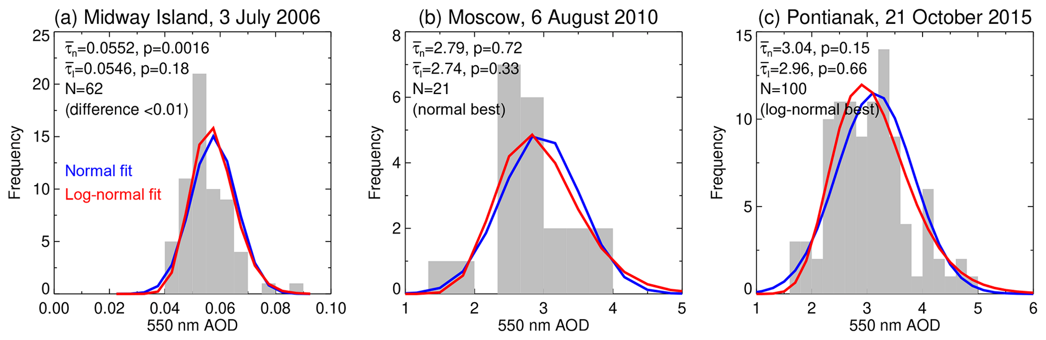
Figure 5Histograms (grey) of 550 nm AOD observed at three AERONET sites on individual dates (given in panel titles), corresponding to different SW test classification results. Arithmetic- and geometric-mean AOD (, respectively), p values for the SW test for the respective distributions, number of points, and category are also given for each case. Bin sizes are site-dependent. Normal and log-normal fits to each histogram are shown in blue and red, respectively.
Days where neither normal nor log-normal distributions provide a good fit to AOD observations are commonly those where multiple regimes are present within a grid cell or during a day. Figure 6 presents a case study from the AERONET site in Essex, Maryland, USA, on 5 July 2011. This day was previously analysed by Eck et al. (2014) as a case of rapid AOD enhancement following the development of a cumulus cloud field just after 17:00 UTC (universal time coordinated), near solar noon (Fig. 6a). The Sun photometer was operated with a 3 min sampling cadence, with 132 points in total throughout the day. For the day as a whole, p(τ)≪pt and p(log 10τ)≪pt; i.e. the data are inconsistent with both normal and log-normal distributions, revealed by the bimodality of the histogram in Fig. 6b. However, for the 111 points before 17:00 UTC p(τ)=0.002 and p(log 10τ)=0.009, and for the 14 points after 18:00 UTC, p(τ)=0.38 and p(log 10τ)=0.54, in both cases indicating stronger evidence for log-normality than normality. By combining various data sets and lines of evidence, Eck et al. (2014) attribute enhancements like these to a combination of humidification and new particle formation rather than cloud contamination in the direct-Sun data, so there is physical reasoning for this bimodality. In situations like this the multimodal-fitting approach of Povey and Grainger (2019) would give a more complete representation of the aerosol field than presenting single-distribution summary statistics. Distribution-agnostic metrics (such as reporting various percentiles of the AOD) are an alternative option.
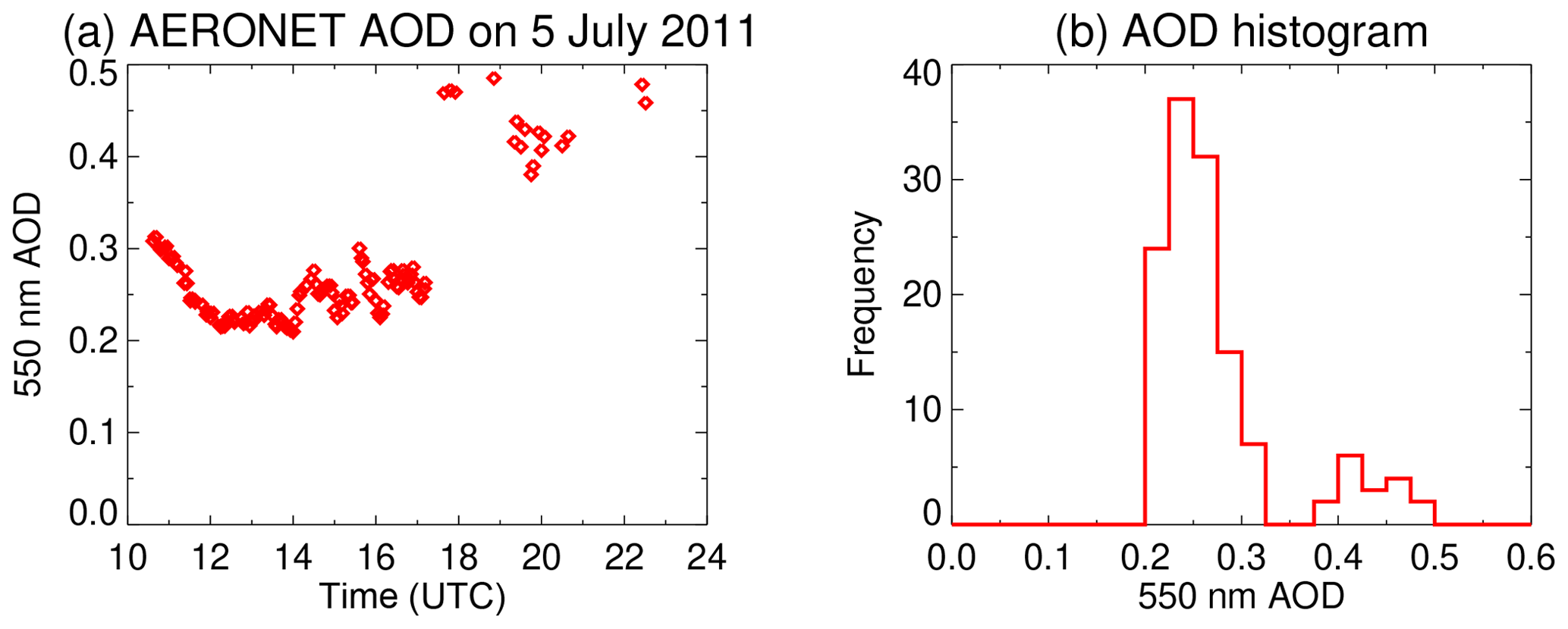
Figure 6(a) Time series and (b) histogram (bin size 0.025) of 550 nm AOD observed at the Essex, Maryland, AERONET site on 5 July 2011.
Note also that the near-universal choice of aggregating daily on a UTC calendar day basis, rather than in terms of local solar time (LST), can further complicate matters for locations far from the meridian. For example, AERONET sites in eastern Asia, Australasia, and the western Americas often contain data from midnight to mid-morning UTC, with a long gap, and then from late evening to midnight UTC. The break in the middle is due to local nighttime, during which no data are collected; i.e. observations from a single UTC day can contain data from 2 local days. If something happens during this gap to affect the AOD distribution, which is often the case due to the diurnal variations or meteorology, this will naturally increase the chances of multimodality. Thus, something as basic as the definition of the day to aggregate to can affect the inferred AOD distribution shape. This could be contributing to some of the cases where neither distribution fits (Figs. 3 and 4) in these parts of the world. This affects all the data sets. This issue has also been explored by Schutgens et al. (2016b), examining the correlation between hourly and daily modelled AOD fields for two different definitions of a day (UTC vs. LST).
While similar, the patterns in Figs. 3 and 4 are not identical between data sets. G5NR is the only data set which enables both spatial and temporal aggregation on a daily basis. Here, both aggregates show, for example, small differences between and over much of the global ocean and a higher frequency of large differences over southern and eastern Asia. However, the spatial aggregates also show areas of large difference (fit well by neither normal nor log-normal distributions) for grid cells with strong elevation variations, such as along the edges of the Himalayas or Andes, while the temporal aggregates do not. If the bulk of the aerosol here is low-lying, then this naturally leads to another case of multiple populations within a grid cell. This is not seen to the same extent in the satellite retrievals here, although they are known to undersample (due to misinterpreting spatial heterogeneity of the scene for cloud cover) and sometimes have retrieval artefacts which could distort the distributions (Zelazowski et al., 2011; Sayer et al., 2014; Loría-Salazar et al., 2016). In these cases moving to a finer spatial scale might be useful to provide summary metrics for these populations separately; i.e. 1∘ might be too coarse. The aforementioned retrieval artefacts might also explain some of the discrepancies between MODIS and other results in other mountainous areas such as western North America, Europe, and the Horn of Africa.
G5NR temporal aggregates also show increased incidence of log-normality and of neither distribution fitting well in the Southern Ocean, while G5NR spatial aggregates do not; this implies diurnal cycles which affect the aerosol field here coherently on scales larger than 1∘. A similar feature, with 10 %–20 % occurrence of normally distributed AOD in the Southern Ocean, is seen in the MODIS results. MODIS retrievals are known to report higher AOD here than other data sets (including active sensors, Sun photometry, and data sets with stricter cloud screening); Toth et al. (2013) attributed much of this to a combination of cloud contamination and retrieval assumptions of surface wind speed (which affect surface brightness). This latter factor was addressed in more recent MODIS data versions (Levy et al., 2013) compared to those used by Toth et al. (2013), although the enhanced AOD remains, implying that cloud contamination is still a factor. A similar enhancement was seen in older version of the MISR data product but largely removed in the latest version used here (Witek et al., 2018). This implies that the occasional normality seen in MODIS daily AOD in the Southern Ocean is likely to be an artefact of biases in the AOD retrievals. MODIS and MISR also report normal or log-normal AOD distributions each up to about 30 % of the time over various North African and Central Asian deserts, while G5NR does not. Unfortunately, the remoteness of many of these areas means that AERONET has few sites in them. It is therefore hard to resolve the reasons for differences between the various data sets.
Table 2Fractional SW test assignment of spatial AOD variation with a day from selected AERONET DRAGON-like deployments and clustered sites.
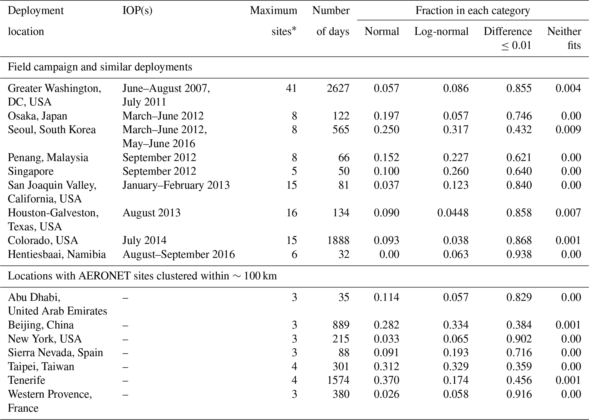
∗ Maximum number of sites providing data on a single day may be less than number of sites deployed in total.
AERONET also provides some opportunities to study the spatial distribution of AOD on horizontal scales of tens of kilometres to around 100 km, similar to L3 and global-climate-model resolution. These are mostly in so-called Distributed Regional Aerosol Gridded Observation Networks (DRAGONs) of up to several dozen sites, as detailed by Holben et al. (2018), deployed during intensive operating periods (IOPs) of field campaigns. Some DRAGON deployments have been in areas also containing several long-term AERONET sites (e.g. those around Washington, DC, USA), enabling spatial characterisation (to a lesser extent) outside these IOPs. Furthermore, a few areas have had three or more AERONET sites deployed simultaneously within ∼100 km of each other; often (but not always) this overlap was temporary as one site replaced another. Table 2 shows the categorisation resulting from applying the SW and AOD difference threshold tests on daily geometric-mean AOD for each of these field campaign deployments or groups of spatially clustered AERONET sites. More details of the DRAGON deployments are available in Holben et al. (2018), and the AERONET web page (https://aeronet.gsfc.nasa.gov, last access: 14 November 2019) provides additional background information and the locations of other clustered sites. Categorisation results are broadly in line with Figs. 3 and 4, and Table 1, in that typically the most common finding is that the difference between daily arithmetic- and geometric-mean AOD is smaller than 0.01. For the 10 field campaign deployment regions listed in Table 2, log-normality is more commonly observed than normality in 6 of them for the days when the resulting difference in AOD is at least 0.01. For the seven clusters of sites outside of field campaigns (which have fewer, i.e. three to four sites total), log-normality is more common in five. While this is consistent with the picture from the larger-scale analysis, it is also important to recall that these deployments are typically short in time (often weeks to months) and tend to be around major metropolitan areas. As a result the frequencies in Table 2 might not be extensible to longer time periods at these locations or other environments.
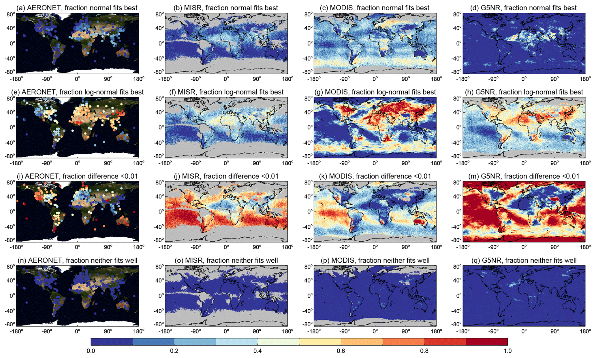
Figure 7As in Fig. 3 except for AOD distributions aggregated temporally from daily to monthly. Columns show (from left to right) AERONET, MISR, MODIS, and G5NR data. Except for G5NR, at least 16 contributing months are required for an AERONET site or grid cell to be valid; grid cells with insufficient data are shaded in grey.
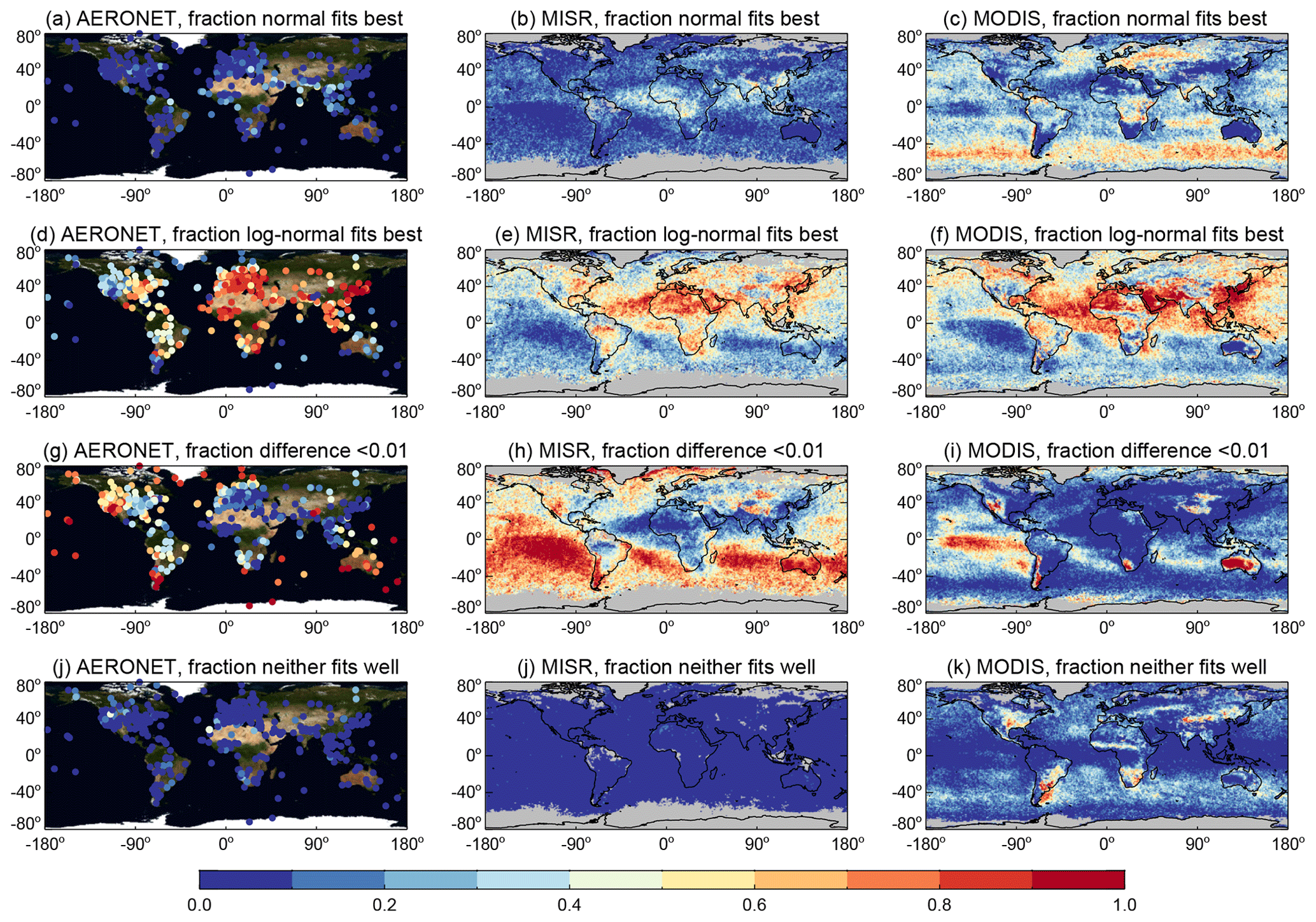
Figure 8As in Fig. 3 except for AOD distributions aggregated temporally from daily to seasonal. Columns show (left) AERONET, (middle) MISR, and (right) MODIS data. At least eight contributing seasons are required for an AERONET site or grid cell to be valid; grid cells with insufficient data are shaded in grey.
3.2 Temporal variation on monthly and seasonal scales
Maps of categorisation of monthly and seasonal AOD aggregates, in both cases from daily AOD, are shown in Figs. 7 and 8, respectively. Global-average fractions are again shown in Table 1. Monthly satellite and AERONET composites require at least 16 contributing months to be considered valid, and seasonal composites require at least eight contributing seasons; for the satellites, using 5 years of data, a maximum of 60 months or 15 seasons are possible. Increasing these thresholds removes some shorter-term AERONET sites and satellite retrievals at high latitudes and some tropical locations, where retrieval coverage is limited. As only 1 year of G5NR data are used, the monthly analysis is performed but seasonal analysis is not. Moving from daily to monthly aggregates in Table 1, the overall tendency is for AOD differences to become larger (i.e. the fraction within the category decreases), and the distributions increasingly favour log-normality over normality. Going from monthly to seasonal, the trend is more pronounced both in the absolute fraction of data (Table 1) and in the spatial distributions (Fig. 8). As in the daily data, some features are broadly consistent between the data sets.
-
Unlike daily aggregation, for monthly or seasonal aggregation the difference between arithmetic and geometric means is frequently more than 0.01. Thus, monthly and seasonal aggregates are more sensitive to the choice of averaging method. This implies generally larger variability on timescales of months and seasons than of spatial variability within a day, which is consistent with previous work (e.g. Schutgens et al., 2017) that has established that temporal colocation on daily, rather than monthly, timescales is important in reducing sampling-related differences between AOD data sets.
-
The exception to the above is very clean areas that are parts of the open ocean, Australasia, and mountainous or remote continental areas, which are outside of aerosol transport paths. Here, for much (but not always a majority) of the time, the AOD difference remains less than 0.01.
-
Downwind of major aerosol source regions, over both and land and ocean, all data sets tend to report higher consistency more frequently with log-normal than with normal distributions.
Some of the differences between the data sets identified in the daily analysis, such as the Southern Ocean AOD in MODIS, are still present in the monthly and seasonal analyses. While patterns are often consistent, differences in magnitudes of each category may be driven in part by sampling differences, which are more pronounced at these scales. Of up to 31 d contributing to a month and 92 d to a season, AERONET and MODIS often sample ∼10–25 and 20–70, respectively (dependent on cloud cover and polar night), while MISR (due to its narrower swath) often samples only 3–7 d per month and 5–15 d per season. Dependent on the temporal scales of aerosol system change, these differences may be important. This limited sampling accounts for the sparser MISR coverage at high latitudes in Fig. 7. Monthly and seasonal data are not affected by the same potential “definition-of-day” issues as identified for daily composites. Seasonal aggregates may, however, be influenced by definition of seasons, and in some parts of the world (e.g. southern and eastern Asia due to their summer monsoons at various points from May to September; Kang et al., 1999) definitions other than the canonical DJF, MAM, JJA, and SON used here may be more appropriate.
4.1 Magnitude differences between arithmetic-mean and geometric-mean AOD
The previous portion of the analysis focuses mostly on the occurrence and distinguishability of normal and log-normal distributions for AOD; also relevant are the magnitudes of the differences introduced into the data sets by the choice of averaging method and summary statistic. Figure 9 shows the difference between geometric- and arithmetic-mean AOD () binned as a function of arithmetic-mean AOD, on daily and monthly timescales, from the four data sets. For the daily plots the G5NR temporal aggregation is shown, although results are similar for the spatial aggregation. Also shown in both panels is the Global Climate Observing System (GCOS) goal uncertainty in AOD for an aerosol climate data record (CDR), which is the greater of 0.03 or 10 % of the AOD (GCOS, 2011). AOD differences approaching or exceeding this level imply that the aggregation method alone causes a sensitivity of similar magnitude to the total desired uncertainty and therefore that if data are to be aggregated, then the choice of an appropriate technique is crucial.
It is important to realise that the AOD difference is always zero or negative, as geometric means are always smaller than or equal to arithmetic means (Cauchy, 1821). This means that the offsets will always be systematic. For daily data (left panel of Fig. 9), the median offset, and its dependence on AOD, are reasonably consistent between all four data sets. The central 68 % of the observed offsets are also somewhat smaller than the GCOS uncertainty requirement and below a total AOD of around 0.6, generally smaller than 0.02.
Even a small offset in reported AOD, if systematic, can have important implications for calculations of climate forcing. This is particularly true for aerosol–cloud interactions, as these are very sensitive to both the anthropogenic perturbation and the natural background state assumed. For example, using perturbed parameter simulations to global climate models, Carslaw et al. (2013) estimated that 45 % of the uncertainty in the global mean forcing due to the cloud albedo effect of aerosols was related to uncertainties in the natural background aerosol burden, compared to 34 % for anthropogenic emissions. Others, including Penner et al. (2011) and Grandey and Wang (2019), have similarly found large dependence of forcing depending on the choice of background. Where AOD is low, such as over much of the global ocean, a small absolute AOD change can be a large relative perturbation. Although the limitations of satellite retrievals for some of these applications are well-known (e.g. Penner et al., 2011; Stier, 2016), the same argument may apply if forcing parametrisations are developed from model simulations aggregated in certain ways. As a result, even differences smaller than the GCOS goal uncertainty, such as the daily differences in Fig. 9, may be significant for these purposes. To paint a more complete picture of the forcing, ideally the overall shape of the distribution, rather than a single number, should be considered; this has also been found to be important for parametrisations related to the cloud radiative effect (Chen et al., 2019) and rainfall (Vlc̆ek and Huth, 2009).
In contrast to the daily results, and even in low–moderate AOD loadings around 0.3, for monthly aggregates (right panel of Fig. 9) the difference is often similar to or larger than this GCOS uncertainty. This means that the choice of arithmetic- or geometric-mean AOD as a summary metric in itself can and often does introduce systematic offsets in reported monthly AOD of a similar size to the goal total uncertainty for an AOD CDR. While this is not strictly an error (in the mathematical sense), if the analyst is using the arithmetic mean as a summary of log-normally distributed data, then, as stated earlier, the inferred typical (common) level of AOD will be biased. Inferences made may be misleading, and less complete, than those if the shape and width of the distribution were considered explicitly. As with the daily data, the magnitude of the offset is AOD-dependent; the magnitude is, however, less consistent than for the daily results, with the median offset being largest for AERONET. This might in part reflect known tendencies for a high bias in low-AOD conditions and/or low bias in high-AOD conditions in these satellite products (Kahn et al., 2010; Eck et al., 2013; Levy et al., 2013; Sayer et al., 2019), meaning that the difference is dampened due to diminished spatial and temporal variability within and between days. The asymmetry of the variabilities (vertical lines) in both panels of Fig. 9 indicates a dependence of the difference on the specific local conditions, i.e. the factors affecting the width of the distribution.
As Fig. 9 established that on monthly timescales sensitivities to averaging method often exceed GCOS goal CDR uncertainties, and Fig. 10 maps how frequently such exceedances occur. The behaviour for seasonal aggregates (not shown) is more pronounced than that of monthly and shows similar spatial features. As seen in earlier parts of this study, the four data sets give broadly consistent spatial patterns but differences in magnitude. Specifically, this is seen most frequently (30 %–90 %, dependent on grid cell and data set) in eastern Asia and Saharan outflow regions, which is unfortunate because these are important and frequently studied components of the global aerosol system. Exceedance of GCOS thresholds in 10 %–40 % of months is also seen fairly consistently across much of eastern North America and Eurasia, South America, southeastern Asia, and southern Africa. This is most common during the summer months (former two cases) and local biomass-burning seasons (other cases), when AOD levels are generally higher. GCOS threshold exceedance is infrequent (observed <10 % of the time) over the remote open ocean in any of the data sets, although they may be slightly elevated for oceanic regions downwind of continental aerosol sources. In all of these regions, the monthly data show higher consistency with log-normality more often than they do than normality (Fig. 7), particularly for the AERONET record, which has the most reliable AOD. Therefore, the locations where the difference between and is largest are also generally those where the data support log-normal summary statistics the most.
A potential counterexample to the need to account for distribution shape is the case of particulate matter (PM) estimation from AOD retrievals, in which case it might be more sensible to report arithmetic-mean AOD than the geometric-mean AOD, even if the underlying distribution is log-normal. This is because the arithmetic mean is directly proportional to the total, while the geometric mean requires knowledge of distribution width as well to return total mass, and in PM studies it is often the total mass which is of interest. However, in practical terms, PM forecasts and nowcasts and daily exposure estimates typically use the finest resolution data available rather than aggregates (Lee et al., 2016). Still, this may be relevant for long-term studies looking at total PM exposure levels, which are often finely spatially resolved but are aggregated temporally (van Donkelaar et al., 2016).
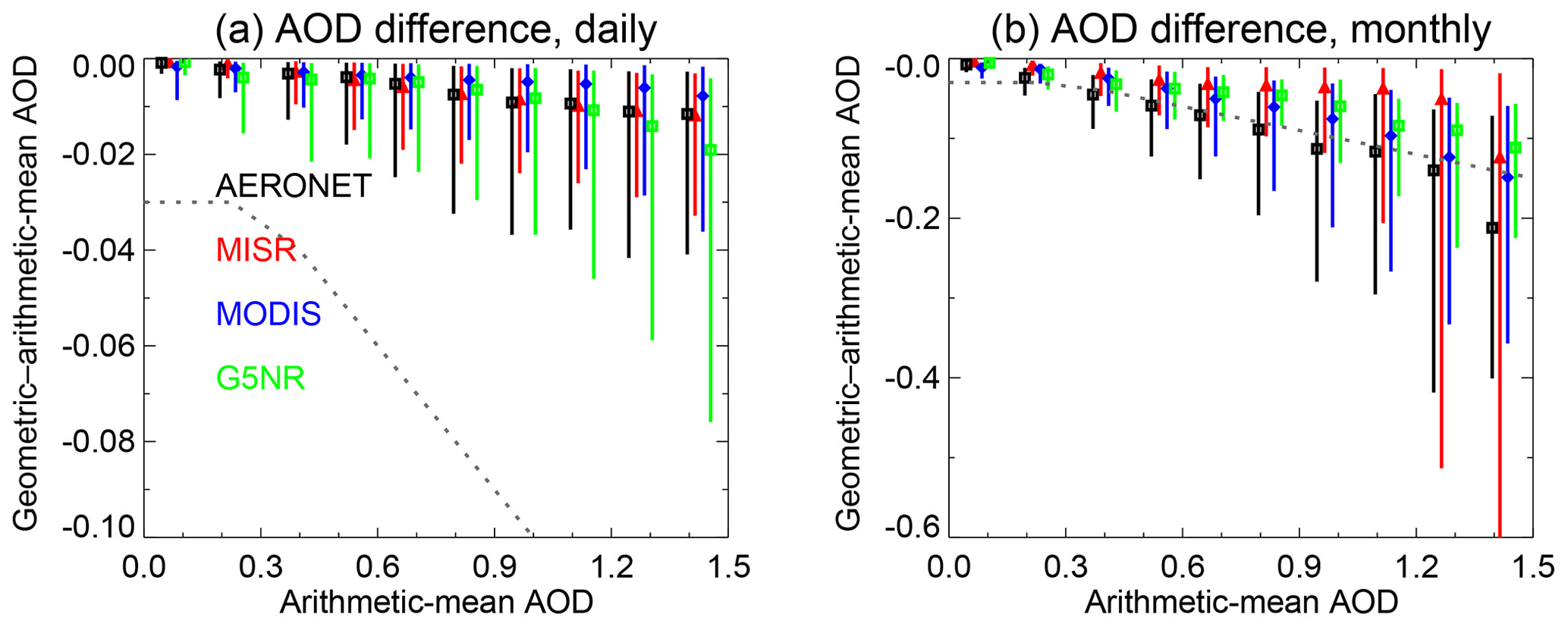
Figure 9Median (symbols) and central 68 % (lines) of binned difference between geometric- and arithmetic-mean AOD () on daily (a) and monthly (b) timescales. Colours indicate AERONET (black), MISR (red), MODIS (blue), or G5NR (green) data. The AOD bin size is 0.15; data sets are horizontally offset slightly for clarity. The dashed grey lines indicate the GCOS goal AOD uncertainty of the maximum of 0.03 or 10 %.
The issue may also be less crucial in analyses where the purpose is to assess the offsets between two data sets (e.g. difference between L3 composites), as opposed to the geophysical fields themselves, as differences between the arithmetic means of two data sets and geometric means of the same two data sets are likely to be of the same sign. The magnitudes will, however, differ depending on the tails of the distributions. As indicated earlier, for AOD, sampling differences between data sets can often be a large determinant of observed offsets (Levy et al., 2009; Sayer et al., 2010; Schutgens et al., 2016b, 2017). Still, examining multiple differences (e.g. differences between arithmetic means, between geometric means, and median differences) can be informative with respect to how much the distributions are influenced by outliers and as a general indicator of skew. Examples include Fig. 2 of Hsu et al. (2012) or Fig. 11 of Sayer et al. (2014).
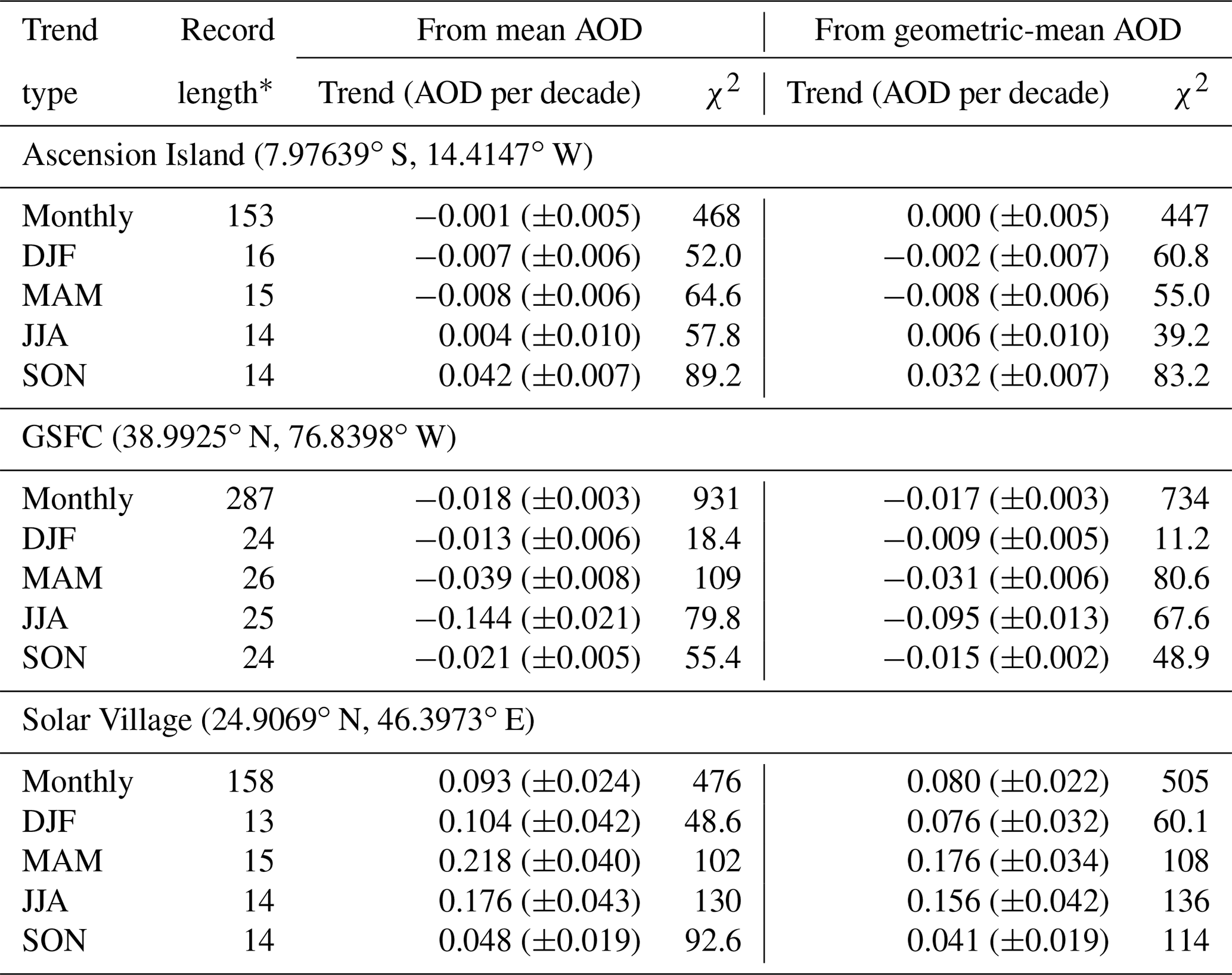
Table 3Decadal trends (±1σ uncertainty estimates) in AERONET AOD at 550 nm, estimated using arithmetic- and geometric-mean AOD as a basis for time series.
∗ Number of contributing months for the monthly time series, and number of contributing years for the seasonal time series.
4.2 Implications for AOD trend analyses
As the differences between arithmetic and geometric mean are larger for higher-AOD regions (Figs. 9 and 10), choice of summary statistic could also influence the calculation of AOD trends. Specifically, as by an increasing amount as AOD increases, smaller magnitudes of calculated trends would be expected (as the maxima are dampened to a higher degree than the minima). Multiple studies over the past few decades have looked at AOD trends globally and regionally, whether over oceans only (e.g. Mishchenko and Geogdzhayev, 2007; Zhao et al., 2008; Thomas et al., 2010; Zhang and Reid, 2010; Li et al., 2014a) or both oceans and land (e.g. Hsu et al., 2012; Chin et al., 2014; Li et al., 2014b; Yoon et al., 2014; Pozzer et al., 2015; Klingmüller et al., 2016). While data sources, periods of analysis, and analysis techniques differ, as do quantitative results, several features tend to be consistently reported.
-
AOD over the global ocean, and over many ocean basins, has not changed very much.
-
AOD over parts of eastern North America and Europe has decreased in recent decades.
-
Some of the strongest positive AOD changes tend to be seen over the Arabian Peninsula.
Using three long-term AERONET sites (one for each of the above features), Table 3 provides decadal AOD trends calculated using geometric-mean AOD and arithmetic-mean AOD as a basis. These sites were used in some of the above studies to complement satellite retrieval and model-simulation analyses; in all cases, those studies used arithmetic-mean AOD. Ascension Island is in the South Atlantic Ocean, where reported AOD trends are typically small, and presently has data available from 1998 to 2016. The Goddard Space Flight Center (GSFC) in Maryland, USA, a region of decreasing AOD, has data from 1993 onwards and is one of the longest-running AERONET sites; Solar Village (operated from 1999 to 2013) was at a solar-power farm northwest of Riyadh, Saudi Arabia, and near the maximum of AOD trends reported in previous studies. At these sites, on monthly timescales, the data fell more often into SW category 4 (AOD difference is larger than 0.01, and data are most consistent with draws from a log-normal distribution) 40 %, 61 %, and 70 % of the time for Ascension Island, GSFC, and Cabo Verde, respectively, than category 3 (more consistent with draws from a normal distribution). In most cases the bulk of the remainder of months fell into category 1 (AOD difference smaller than 0.01). On a seasonal basis this preference for log-normality over normality is even more pronounced, corresponding to 68 %, 79 %, and 82 % of the time to category 4, respectively.
The purpose here is not to perform an exhaustive global trend analysis but to assess quantitatively the implications of log-normally distributed AOD on some well-reported features of global aerosol trends. Prior studies typically calculated trends based on deseasonalised monthly mean AOD time series and calculating a linear least-squares regression fit. Deseasonalisation was achieved either by subtracting the mean AOD annual cycle over the time period or, as in Thomas et al. (2010) and Klingmüller et al. (2016) by using harmonic regression to model the annual cycle. Li et al. (2014a, b) took a somewhat different approach by analysing the temporal variability in principal components of monthly AOD fields rather than the AOD fields themselves. In some of these analyses, seasonal trends were calculated by averaging the monthly data within each season, although in this case it is arguably more reasonable to use seasonal aggregates from daily data as a basis. The motivation for considering seasonal trends is that some aerosol features, and their variability, are characteristic of particular seasons (e.g. Ascension Island and GSFC sample transported smoke through summer and autumn but seldom during other seasons; at Solar Village dust storms are most frequent and intense in spring and summer).
Here, linear trends are calculated using both monthly and seasonal aggregates for both normal (i.e. arithmetic mean) and log-normal (i.e. geometric mean) aggregates, both calculated from daily AOD ( or , respectively). Monthly trends are calculated using the monthly AOD time series, after subtraction of the mean seasonal cycle, as in previous studies. Seasonal trends do not require a deseasonalisation step. The data are fit using linear least-squares regression, with the weights equal to the standard error on the estimated monthly (or seasonal) AOD. For the log-normal averaging this is strictly asymmetric, although it is approximated as symmetric in this case, which has negligible influence on the results. The lower limit for these standard errors is taken as 0.01, corresponding to the AERONET AOD uncertainty. As this is largely dominated by calibration uncertainty (Eck et al., 1999), it is not significantly reduced by averaging and can therefore be considered systematic over a single (roughly year-long) deployment but closer to random over a multi-year time series. The standard error on the annual cycle is added in quadrature to the estimated uncertainty in the monthly time series to account for the uncertainty in the deseasonalisation step. Following Weatherhead et al. (1998), the lag-1 autocorrelation is estimated and used to adjust the uncertainty estimates. Furthermore, the χ2 statistics on the fits, which have an expected value of n−2 (where n is the record length and two parameters are fit in the regression), were in most cases somewhat in excess of this (Table 3). This implies that the standard errors are not a complete representation of the uncertainty in the time series data and/or that a linear model does not fully describe the variation. Thus, in addition to the autocorrelation correction, the trend uncertainty estimates in Table 3 are also scaled by .
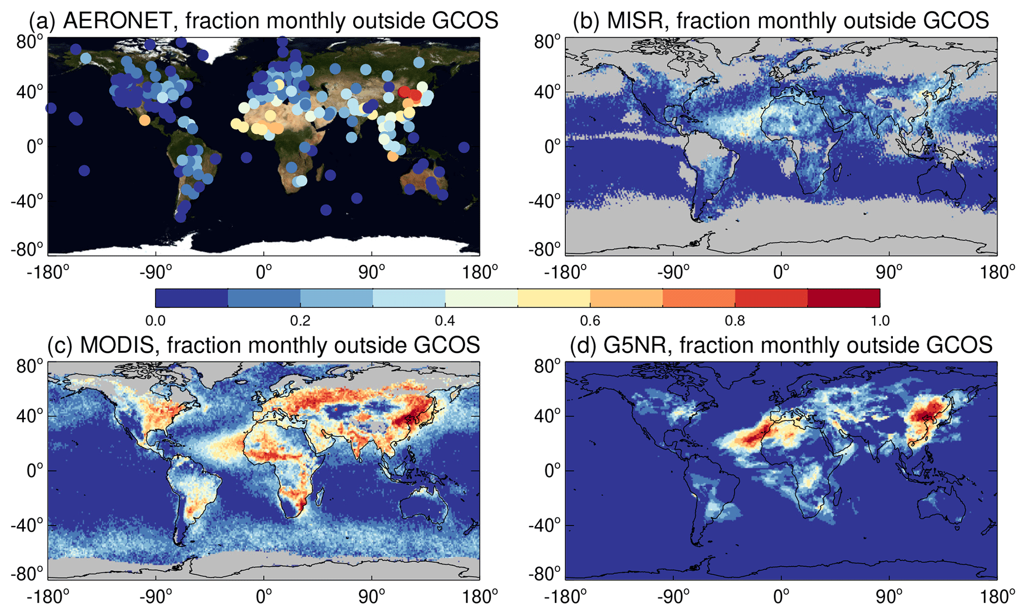
Figure 10Fraction of months where the difference between arithmetic- and geometric-mean AOD is larger than the GCOS goal uncertainty for an AOD climate data record; i.e. . Panels show results for (a) AERONET, (b) MISR, (c) MODIS, and (d) G5NR.
At each of the three sites, the decadal AOD trends are qualitatively the same whether calculated using arithmetic- or geometric-mean AOD time series as a basis. However, as expected, trends using geometric-mean AOD are smaller in magnitude (i.e. increases and declines in AOD are less pronounced). The decrease in magnitude is often of the order of 10 %–30 %, which is typically within the 1σ uncertainty estimates on the calculated AOD trend. The implication of this is that, as a result of assuming an underlying normal distribution, prior studies may be qualitatively correct on the sign of AOD trends but quantitatively have a tendency to overestimate their magnitude (again using the prior definition of “typical” or “common” aerosol loading). For log-normally distributed data, trends in geometric quantities are more straightforward to interpret.
Note that during presentations and reviews of this work, a question arose as to whether, moving from point trends to larger regional-scale trends, the central limit theorem (CLT) would mean that arithmetic and geometric trends would converge. The CLT does not imply that expanding the region (adding more data) means that the AOD would become closer to a normal distribution; this is a common misconception of the CLT. Rather, the uncertainties on estimates of the summary statistic (whether arithmetic or geometric means) will behave approximately according to normal statistics, even if the underlying AOD distribution is not normal. It does not mean that the underlying quantity becomes closer to normally distributed; this misconception of the CLT is discussed in Sect. 3.1.3 of the review by Sotos et al. (2007). The answer therefore depends on the form of distributions in space and time across the region (as well as, potentially, the order in which the data are averaged). As the evidence from data sets in this analysis (Figs. 3, 4, 7, and 8) indicates that on larger scales AOD data become increasingly often more consistent with the log-normal than the normal distribution, and this was also found by prior spatial analyses (Ignatov and Stowe, 2000), it seems likely that regional-scale (rather than point) AOD trend estimates would show similar, or even accentuated, differences between trends in arithmetic- and geometric-mean trends.
4.3 Summary and recommendations for data use
Widely used spatiotemporal aggregates of aerosol data from surface observations, satellite retrievals, and model simulations typically consist of arithmetic means and standard deviations of finer-resolution data. These statistics are most meaningful for normally distributed data, while previous work has indicated that AOD is often distributed close to log-normally on large scales. While one can transform between normal and log-normal summary statistics (e.g. Table 1 of O'Neill et al., 2000), in practice it is typical for data users to (implicitly or explicitly) assume normality in their analyses without considering the underlying distribution shape. This can influence the inferences drawn from the data. This study has illustrated the use of Shapiro–Wilk tests as a comparative tool to assess whether quantities such as AOD are more consistent with draws from normally or log-normally distributed populations. Data from ground-based observations (AERONET), satellite retrievals (MISR and MODIS), and model simulations (G5NR), despite their varying sampling and error characteristics, provide broadly consistent results.
As timescales increase from days to months to seasons, data become increasingly more consistent with log-normal than normal distributions, and the differences between arithmetic- and geometric-mean AOD become larger; assuming normality systematically overstates both the typical level of AOD and its variability. In low-AOD regions such as the open ocean and mountains, often the AOD difference is small enough (<0.01) to be unimportant for many applications especially on daily timescales. However, in continental outflow regions and near source regions over land, and on monthly or seasonal timescales, the difference is frequently larger than the GCOS goal uncertainty in a climate data record (the larger of 0.03 or 10 %). As a result of this, estimated trends in geometric-mean AOD are smaller in magnitude than (although consistent in sign with) those in arithmetic-mean AOD.
As noted earlier, using the arithmetic mean and standard deviation to summarise log-normal data is not “wrong” in a mathematical sense, as one can transform between the two. The danger is in not explicitly considering the underlying distribution when drawing an inference, as the result may be misleading or, at a minimum, less of a full picture than could otherwise be obtained.
The main recommendations from this study for future missions and reprocessing of current data sets and simulations are as follows.
-
The frequency distribution of a geophysical quantity should be analysed in order to assess how best to aggregate it. This analysis should be done at the spatial and temporal scale or scales of interest for the aggregation because distributions are scale-dependent. The Shapiro–Wilk technique is a powerful tool to assess discrepancies from a normal or log-normal distribution and should be further combined with desired performance thresholds to assess whether discrepancies are scientifically relevant for a given quantity.
-
Ideally AOD aggregates such as satellite L3 products, but also from ground-based (e.g. AERONET) and model simulations, should report geometric-mean or median AOD rather than (or in addition to) arithmetic-mean AOD. Where data sets permit zero or unphysical negative AOD values (incompatible with geometric calculations), these should be truncated to some reasonable lower bound which will not introduce meaningful artefacts in derived statistics (such as 0.0001 used here for MODIS and MISR). These summary statistics are relevant because multiple data records provide evidence that AOD distributions are generally closer to log-normal than normal, particularly on monthly and seasonal timescales, and the geometric mean is the more natural and meaningful summary statistic for such data. This information should be clearly communicated to potential data users. Geometric mean AOD is systematically lower, often (on monthly or seasonal timescales) by more than the GCOS goal climate data record uncertainty of the larger of 0.03 or 10 %, so the choice of averaging method is scientifically important.
-
Due to the computational burden required on the data producer or user's end (i.e. for satellites; obtaining the full L2 data record to reaggregate to daily and then monthly time steps), this is unlikely to happen in the short term. In the meantime, calculation of geometric-mean monthly aggregates from current standard (i.e. arithmetic mean) daily L3 aggregates could be a useful stopgap measure. This is because the volume of daily L3 data is smaller than L2, and daily spatial aggregates were found to be less sensitive than monthly ones to the choice of arithmetic vs. geometric averaging.
-
Comparisons and statistical assessments of AOD must account for the expected numerical distribution. Some common performance assessment techniques making use of sum-of-squares calculations, such as the root-mean-square error or coefficient of determination, should not be used in all cases, as they can be systematically skewed by large tails on non-normally distributed data (Seegers et al., 2018). Consequently, dependent on the magnitudes of errors and the range of AOD observed, their interpretation can be less meaningful if one does not also look at the underlying data.
The analysis presented here refers to AOD, but the methodology is general. GCOS (2011) provide goal uncertainties for many geophysical CDRs, which may be helpful for assessing the importance of averaging method in different disciplines. Overall the log-normal distribution seems to be a better reference for AOD aggregates than the normal distribution, on spatial scales of single locations or 1∘ and temporal scales from days to seasons.
It is important to bear in mind that these simple distribution forms are just approximations for the true underlying distribution of a geophysical quantity, and the relevant problem is in identifying one which is a sufficiently accurate representation for a given task. Normal and log-normal distributions are mathematically convenient and represent many data sets reasonably well, which is a motivating factor for considering these two both historically and in the present work. Sometimes multiple distribution forms are suitable: this analysis has shown that often in low-AOD conditions the choice of normal or log-normal representation may not matter for many purposes. Furthermore, while not analysed here, dependent on the choice of parameters, gamma distributions (often used to describe cloud particle size distributions, e.g. Platnick et al., 2017) can be numerically similar to log-normal ones. Indeed, both gamma and log-normal distributions can provide good summaries of rain rates in some circumstances (Cho et al., 2004; Vlc̆ek and Huth, 2009). Sometimes multiple modes are required, and sometimes neither distribution is a suitable approximation.
If only a few distributions or points need to be summarised, then it is of course preferable to show the actual distributions and/or an informative summary which is agnostic to any particular distribution shape, such as a box-and-whisker plot. However for many larger-scale analyses, aggregated outputs from observations and model simulations are likely to remain the format of the choice for many data users due to their convenience and significantly lower computational and storage requirements than full-resolution (e.g. L2) data. While these unavoidably lead to a loss of information, it is important that users consciously consider the underlying distributions that the data sets are drawn from when utilising these summary statistics in research. The above recommendations will result in more statistically and scientifically meaningful data sets and decrease potential systematic biases which can lead to erroneous qualitative and quantitative interpretation about the state of the Earth system.
The geometric-mean AOD output presented in this work is available upon request to the authors. AERONET data are available from https://aeronet.gsfc.nasa.gov (last access: 14 November 2019. NASA AERONET team, 2019). MISR and MODIS data are available from https://earthdata.nasa.gov (last access: 14 November 2019. NASA EarthData portal team, 2019), and G5NR simulation output is available from https://g5nr.nccs.nasa.gov/data/ (last access: 14 November 2019. NASA GMAO, 2019).
AMS and KDK jointly conceptualised the analysis. AMS performed the analysis and drafted the paper. Both authors contributed to the editing of the text.
The authors declare that they have no conflict of interest.
This research was performed as part of the NASA Plankton, Aerosol, Cloud, ocean Ecosystem (PACE) mission development. The AERONET team and site principal investigators and managers are thanked for the creation and maintenance of the AERONET data record. Satellite retrieval and modelling teams, and hosting entities, are acknowledged for the development and archiving of these data sets. Tom F. Eck (USRA), Brent N. Holben (NASA GSFC), and Alexander Smirnov (SSAI) are thanked for useful discussions about early AOD and turbidity measurement networks and their strengths and limitations. Patricia Castellanos (NASA GSFC) is thanked for advice on the use of the G5NR simulation. Chris J. Merchant (University of Reading) is thanked for input on uncertainty characterisation in sea surface temperature data. This analysis was also presented as part of NASA GSFC's AeroCenter seminar series and to the NASA Ocean Ecology Laboratory. The insightful comments, questions, suggestions, and endorsement of attendees of those seminars, as well as Yilun Chen (USTC), Adam C. Povey (Oxford), and three anonymous reviewers, are appreciated.
This research has been supported by the NASA PACE project.
This paper was edited by Anja Schmidt and reviewed by three anonymous referees.
Ahlquist, N. C. and Charlson, R. J.: Measurement of the wavelength dependence of atmospheric extinction due to scatter, Atmos. Environ., 3, 551–564, https://doi.org/10.1016/0004-6981(69)90045-6, 1967. a
Alexandrov, M. D., Marshak, A., Cairns, B., Lacis, A. A., and Carlson, B. E.: Scaling Properties of Aerosol Optical Thickness Retrieved from Ground-Based Measurements, J. Atmos. Sci., 61, 1024–1039, https://doi.org/10.1175/1520-0469(2004)061<1024:SPOAOT>2.0.CO;2, 2004. a
Alexandrov, M. D., Geogdzhayev, I. V., Tsigaridis, K., Marshak, A., and Levy, R.: New Statistical Model for Variability of Aerosol Optical Thickness: Theory and Application to MODIS Data over Ocean, J. Atmos. Sci., 73, 821–837, https://doi.org/10.1175/JAS-D-15-0130.1, 2016. a
Anderson, T. L., Charlson, R. J., Winker, D. M., Ogren, J. A., and Holmén, K.: Mesoscale Variations of Tropospheric Aerosols, J. Atmos. Sci., 60, 119–136, https://doi.org/10.1175/1520-0469(2003)060<0119:MVOTA>2.0.CO;2, 2003. a, b
Ångström, A.: On the atmospheric transmission of Sun radiation and on dust in the air, Geogr. Ann., 12, 130–159, https://doi.org/10.1080/20014422.1929.11880498, 1929. a
Buchard, V., da Silva, A. M., Colarco, P. R., Darmenov, A., Randles, C. A., Govindaraju, R., Torres, O., Campbell, J., and Spurr, R.: Using the OMI aerosol index and absorption aerosol optical depth to evaluate the NASA MERRA Aerosol Reanalysis, Atmos. Chem. Phys., 15, 5743–5760, https://doi.org/10.5194/acp-15-5743-2015, 2015. a
Bulgin, C. E., Embury, O., Corlett, G., and Merchant, C. J.: Independent uncertainty estimates for coefficient based sea surface temperature retrieval from the Along-Track Scanning Radiometer instruments, Remote Sens. Environ., 178, 213–222, https://doi.org/10.1016/j.rse.2016.02.022, 2016a. a
Bulgin, C. E., Embury, O., and Merchant, C. J.: Sampling uncertainty in gridded sea surface temperature products and Advanced Very High Resolution Radiometer (AVHRR) Global Area Coverage (GAC) data, Remote Sens. Environ., 177, 287–294, https://doi.org/10.1016/j.rse.2016.02.021, 2016b. a
Campbell, J. W.: The lognormal distribution as a model for bio‐optical variability in the sea, J. Geophys. Res., 100, 13237–13254, https://doi.org/10.1029/95JC00458, 1995. a
Carslaw, K. S., Lee, L. A., Reddington, C. L., Pringle, K. J., Rap, A., Forster, P. M., Mann, G. W., Spracklen, D. V., Woodhouse, M. T., Regayre, L. A., and Pierce, J. R.: Large contribution of natural aerosols to uncertainty in indirect forcing, Nature, 503, 67–71, https://doi.org/10.1038/nature12674, 2013. a
Castellanos, P., Da Silva, A. M., Darmenov, A. S., Buchard, V., Govindaraju, R. C., Ciren, P., and Kondraguntha, S.: A Geostationary Instrument Simulator for Aerosol Observing System Simulation Experiments, Atmosphere, 10, 1–36, https://doi.org/10.3390/atmos10010002, 2018. a, b, c
Cauchy, A.-L.: Cours d'analyse de l'École Royale Polytechnique, première partie, Analyse algébrique, Paris, 576 pp., 1821. a
Chen, Y. L., Chong, K. Z., and Fu, Y. F.: Impacts of distribution patterns of cloud optical depth on the calculation of radiative forcing, Atmos. Res., 218, 70–77, https://doi.org/10.1016/j.atmosres.2018.11.007, 2019. a
Chin, M., Diehl, T., Tan, Q., Prospero, J. M., Kahn, R. A., Remer, L. A., Yu, H., Sayer, A. M., Bian, H., Geogdzhayev, I. V., Holben, B. N., Howell, S. G., Huebert, B. J., Hsu, N. C., Kim, D., Kucsera, T. L., Levy, R. C., Mishchenko, M. I., Pan, X., Quinn, P. K., Schuster, G. L., Streets, D. G., Strode, S. A., Torres, O., and Zhao, X.-P.: Multi-decadal aerosol variations from 1980 to 2009: a perspective from observations and a global model, Atmos. Chem. Phys., 14, 3657–3690, https://doi.org/10.5194/acp-14-3657-2014, 2014. a
Cho, H., Bowman, K. P., and North, G. R.: A Comparison of Gamma and Lognormal Distributions for Characterizing Satellite Rain Rates from the Tropical Rainfall Measuring Mission, J. Appl. Meteor., 43, 1586–1597, https://doi.org/10.1175/JAM2165.1, 2004. a, b
Chubarova, N., Nezval', Ye., Sviridenkov, I., Smirnov, A., and Slutsker, I.: Smoke aerosol and its radiative effects during extreme fire event over Central Russia in summer 2010, Atmos. Meas. Tech., 5, 557–568, https://doi.org/10.5194/amt-5-557-2012, 2012. a
Chylek, P., Henderson, B., and Mishchenko, M.: Aerosol radiative forcing and the accuracy of satellite aerosol optical depth retrieval, J. Geophys. Res., 108, 4764, https://doi.org/10.1029/2003JD004044, 2003. a
Colarco, P. R., Kahn, R. A., Remer, L. A., and Levy, R. C.: Impact of satellite viewing-swath width on global and regional aerosol optical thickness statistics and trends, Atmos. Meas. Tech., 7, 2313–2335, https://doi.org/10.5194/amt-7-2313-2014, 2014. a
d'Almeida, G., Koepke, P., and Shettle, E.: Atmospheric aerosols: global climatology and radiative characteristics, A. Deepak Publishing, 561 pp., 1991. a
Dubovik, O., Holben, B., Eck, T. F., Smirnov, A., Kaufman, Y. J., King, M. D., Tanré, D., and Slutsker, I.: Variability of Absorption and Optical Properties of Key Aerosol Types Observed in Worldwide Locations, J. Atmos. Sci., 59, 590–608, https://doi.org/10.1175/1520-0469(2002)059<0590:VOAAOP>2.0.CO;2, 2002. a
Dubovik, O., Li, Z., Mishchenko, M. I., Tanré, D., Karol, Y., Bojkov, B., Cairns, B., Diner, D. J., Espinosa, W. R., Goloub, P., Gu, X., Hasekamp, O., Hong, J., Hou, W., Knobelspiesse, K. D., Landgraf, J., Li, L., Litvinov, P., Liu, Y., Lopatin, A., Marbach, T., Maring, H., Martins, V., Meijer, Y., Milinevsky, G., Mukai, S., Parol, F., Qiao, Y., Remer, L., Rietjens, J., Sano, I., Stammes, P., Stamnes, S., Sun, X., Tabary, P., Travis, L. D., Waquet, F., Xu, F., Yan, C., and Yin, D.: Polarimetric remote sensing of atmospheric aerosols: Instruments, methodologies, results, and perspectives, J. Quant. Spectrosc. Ra., 224, 474–511, https://doi.org/10.1016/j.jqsrt.2018.11.024, 2019. a
Eck, T. F., Holben, B. N., Reid, J. S., Dubovik, O., Smirnov, A., O'Neill, N. T., Slutsker, I., and Kinne, S.: Wavelength dependence of the optical depth of biomass burning, urban, and desert dust aerosols, J. Geophys. Res., 104, 31333–31349, https://doi.org/10.1029/1999JD900923, 1999. a, b, c, d
Eck, T. F., Holben, B. N., Reid, J. S., Mukelabai, M. M., Piketh, S. J., Torres, O., Jethva, H. T., Hyer, E. J., Ward, D. E., Dubovik, O., Sinyuk, A., Schafer, J. S., Giles, D. M., Sorokin, M., Smirnov, A., and Slutsker, I.: A seasonal trend of single scattering albedo in southern African biomass-burning particles: Implications for satellite products and estimates of emissions for the world's largest biomass-burning source, J. Geophys. Res., 118, 6414–6432, https://doi.org/10.1002/jgrd.50500, 2013. a, b
Eck, T. F., Holben, B. N., Reid, J. S., Arola, A., Ferrare, R. A., Hostetler, C. A., Crumeyrolle, S. N., Berkoff, T. A., Welton, E. J., Lolli, S., Lyapustin, A., Wang, Y., Schafer, J. S., Giles, D. M., Anderson, B. E., Thornhill, K. L., Minnis, P., Pickering, K. E., Loughner, C. P., Smirnov, A., and Sinyuk, A.: Observations of rapid aerosol optical depth enhancements in the vicinity of polluted cumulus clouds, Atmos. Chem. Phys., 14, 11633–11656, https://doi.org/10.5194/acp-14-11633-2014, 2014. a, b
Eck, T. F., Holben, B. N., Giles, D. M., Slutsker, I., Sinyuk, A., Schafer, J. A., Smirnov, A., Sorokin, M., Reid, J. S., Sayer, A. M., Hsu, N. C., Shi, Y. R., Levy, R. C., Lyapustin, A., Rahman, M. A., Liew, S.-C., Salinas Cortijo, S. V., Li, T., Kalbermatter, D., Keong, K. L., Yuggotomo, M. E., Aditya, F., Mohamad, M., Mahmud, M., Chong, T. K., Lim, H.-S., Choon, Y. E., Deranadyan, G., Kusumaningtyas, S. D. A., and Aldrian, E.: AERONET remotely sensed measurements and retrievals of biomass burning aerosol optical properties during the 2015 Indonesian burning season, J. Geophys. Res.-Atmos., 124, 4722–4740, https://doi.org/10.1029/10.1029/2018JD030182, 2019. a
Flowers, E. C., McCormick, R. A., and Kurfis, K. R.: Atmospheric Turbidity over the United States, 1961–1966, J. Appl. Meteor., 8, 955–962, https://doi.org/10.1175/1520-0450(1969)008<0955:ATOTUS>2.0.CO;2, 1969. a, b
Forgan, B. W., DeLuisi, J. J., Hicks, B. B., and Rusina, E. N.: Report on the measurements of atmospheric turbidity in BAPMoN, Tech. Rep., World Meteorol. Organ., Geneva, Switzerland, WMO Rep., 94, 1993. a
Garay, M. J., Kalashnikova, O. V., and Bull, M. A.: Development and assessment of a higher-spatial-resolution (4.4 km) MISR aerosol optical depth product using AERONET-DRAGON data, Atmos. Chem. Phys., 17, 5095–5106, https://doi.org/10.5194/acp-17-5095-2017, 2017. a
GCOS: Systematic observation requirements for satellite-based data products for climate, 2011 update, Tech. Rep., World Meteorological Organization, https://library.wmo.int/doc_num.php?explnum_id=3710 (last access: 14 November 2019), climate Observing System report GCOS-154, 2011. a, b
Geogdzhayev, I., Cairns, B., Mishchenko, M. I., Tsigaridis, K., and van Noije, T.: Model‐based estimation of sampling‐caused uncertainty in aerosol remote sensing for climate research applications, Q. J. Roy. Meteor. Soc., 140, 2353–2363, https://doi.org/10.1002/qj.2305, 2014. a
Giles, D. M., Sinyuk, A., Sorokin, M. G., Schafer, J. S., Smirnov, A., Slutsker, I., Eck, T. F., Holben, B. N., Lewis, J. R., Campbell, J. R., Welton, E. J., Korkin, S. V., and Lyapustin, A. I.: Advancements in the Aerosol Robotic Network (AERONET) Version 3 database – automated near-real-time quality control algorithm with improved cloud screening for Sun photometer aerosol optical depth (AOD) measurements, Atmos. Meas. Tech., 12, 169–209, https://doi.org/10.5194/amt-12-169-2019, 2019. a, b
Grandey, B. S. and Wang, C.: Background conditions influence the estimated cloud radiative effects of anthropogenic aerosol emissions from different source regions, J. Geophys. Res.-Atmos., 124, 2276–2295, https://doi.org/10.1029/2018JD029644, 2019. a
Gupta, P., Levy, R. C., Mattoo, S., Remer, L. A., and Munchak, L. A.: A surface reflectance scheme for retrieving aerosol optical depth over urban surfaces in MODIS Dark Target retrieval algorithm, Atmos. Meas. Tech., 9, 3293–3308, https://doi.org/10.5194/amt-9-3293-2016, 2016. a
Hinds, W. C.: Aerosol technology: properties, behavior, and measurement of airborne particles, Wiley Interscience, New York, Chichester, Weinheim, Brisbane, Singapore, and Toronto, 2 Edn., 504 pp., 1999. a
Holben, B. N., Tanré, D., Smirnov, A., Eck, T. F., Slutsker, I., Abuhassan, N., Newcomb, W. W., Schafer, J. S., Chatenet, B., Lavenu, F., Kaufman, Y. J., Vande Castle, J., Setzer, A., Markham, B., Clark, D., Frouin, R., Halthore, R., Karneli, A., O'Neill, N. T., Pietras, C., Pinker, R. T., Voss, K., and Zibordi, G.: An emerging ground-based aerosol climatology: Aerosol optical depth from AERONET, J. Geophys. Res., 106, 12067–12097, https://doi.org/10.1029/2001JD900014, 2001. a, b
Holben, B. N. et al.: An overview of mesoscale aerosol processes, comparisons, and validation studies from DRAGON networks, Atmos. Chem. Phys., 18, 655–671, https://doi.org/10.5194/acp-18-655-2018, 2018. a, b
Hsu, N. C., Gautam, R., Sayer, A. M., Bettenhausen, C., Li, C., Jeong, M. J., Tsay, S.-C., and Holben, B. N.: Global and regional trends of aerosol optical depth over land and ocean using SeaWiFS measurements from 1997 to 2010, Atmos. Chem. Phys., 12, 8037–8053, https://doi.org/10.5194/acp-12-8037-2012, 2012. a, b
Hsu, N. C., Lee, J., Sayer, A. M., Kim, W., Bettenhausen, C., and Tsay, S.-C.: VIIRS Deep Blue aerosol products over land: Extending the EOS long‐term aerosol data record, J. Geophys. Res.-Atmos., 124, 4026–4053, https://doi.org/10.1029/2018JD029688, 2019. a
Ignatov, A. and Stowe, L.: Physical Basis, Premises, and Self-Consistency Checks of Aerosol Retrievals from TRMM VIRS, J. Appl. Meteor., 39, 2259–2277, https://doi.org/10.1175/1520-0450(2001)040<2259:PBPASC>2.0.CO;2, 2000. a, b
Junge, C. E.: The size distribution and aging of natural aerosols as determined from electrical and optical data on the atmosphere, Am. Meteor. Soc. J., 12, 13–25, https://doi.org/10.1175/1520-0469(1955)012<0013:TSDAAO>2.0.CO;2, 1955. a
Junge, C. E.: Air chemistry and radioactivity, Vol. 4 of International Geophysics Series, Academic Press, New York, 382 pp., 1963. a
Kahn, R. A., Gaitley, B. J., Garay, M. J., Diner, D. J., Eck, T. F., Smirnov, A., and Holben, B. N.: Multiangle Imaging SpectroRadiometer global aerosol product assessment by comparison with the Aerosol Robotic Network, J. Geophys. Res., 115, D23209, https://doi.org/10.1029/2010JD014601, 2010. a, b
Kaku, K. C., Reid, J. S., Hand, J. L., Edgerton, E. S., Holben, B. N., Zhang, J., and Holz, R. E.: Assessing the challenges of surface‐level aerosol mass estimates from remote sensing during the SEAC4RS and SEARCH campaigns: Baseline surface observations and remote sensing in the southeastern United States, J. Geophys. Res.-Atmos., 123, 7530–7562, https://doi.org/10.1029/2017JD028074, 2018. a
Kang, I., Ho, C., Lim, Y., and Lau, K.: Principal Modes of Climatological Seasonal and Intraseasonal Variations of the Asian Summer Monsoon, Mon. Weather Rev., 127, 322–340, https://doi.org/10.1175/1520-0493(1999)127<0322:PMOCSA>2.0.CO;2, 1999. a
Kennedy, J. J.: A review of uncertainty in in situ measurements and data sets of sea surface temperature, Rev. Geophys., 52, 1–32, https://doi.org/10.1002/2013RG000434, 2014. a
King, M. D., Byrne, D. M., Reagan, J. A., and Herman, B. M.: Spectral Variation of Optical Depth at Tucson, Arizona between August 1975 and December 1977, J. Appl. Meteor., 19, 723–732, https://doi.org/10.1175/1520-0450(1980)019<0723:SVOODA>2.0.CO;2, 1980. a
King, M. D., Platnick, S., Menzel, W. P., Ackerman, S. A., and Hubanks, P. A.: Spatial and Temporal Distribution of Clouds Observed by MODIS Onboard the Terra and Aqua Satellites, IEEE T. Geosci. Remote, 51, 3826–3852, https://doi.org/10.1109/TGRS.2012.2227333, 2013. a
Kinne, S., Schulz, M., Textor, C., Balkanski, Y., Bauer, S., Berntsen, T., Berglen, T., Boucher, O., Chin, M., Collins, W. Dentener, F., Diehl, T., Eater, R., Feichter, J., Filmore, D., Ghan, S., Ginoux, P., Gong, S., Grini, A., Hendricks, J. E., Herzog, M., Horowitz, L., Isaksen, I. S. A., Iversen, T., Kirkavåg, A., Kloster, S., Koch, D., Kristjansson, J. E., Krol, M., Lauer, A., Lamarque, J. F., Lesins, G., Liu, X., Lohmann, U. Montanaro, V., Myhre, G., Penner, J. E., Pitari, G., Reddy, S., Seland, O., Stier, P., and Takemura, T.: An AeroCom initial assessment – optical properties in aerosol component modules of global models, Atmos. Chem. Phys., 6, 1815–1834, https://doi.org/10.5194/acp-6-1815-2006, 2006. a, b, c
Kirkwood, T. B. L.: Geometric means and measures of dispersion, Biometrics, 35, 908–909, 1979. a
Klingmüller, K., Pozzer, A., Metzger, S., Stenchikov, G. L., and Lelieveld, J.: Aerosol optical depth trend over the Middle East, Atmos. Chem. Phys., 16, 5063–5073, https://doi.org/10.5194/acp-16-5063-2016, 2016. a, b
Kok, J. F.: A scaling theory for the size distribution of emitted dust aerosols suggests climate models underestimate the size of the global dust cycle, P. Natl. Acad. Sci. USA, 108, 1016–1021, https://doi.org/10.1073/pnas.1014798108, 2011a. a
Kok, J. F.: Does the size distribution of mineral dust aerosols depend on the wind speed at emission?, Atmos. Chem. Phys., 11, 10149–10156, https://doi.org/10.5194/acp-11-10149-2011, 2011b. a
Kokhanovsky, A. A. and de Leeuw, G. (Eds.): Satellite Aerosol Remote Sensing Over Land, Springer, Berlin, https://doi.org/10.1007/978-3-540-69397-0, 2009. a
Kovacs, T.: Comparing MODIS and AERONET aerosol optical depth at varying separation distances to assess ground‐based validation strategies for spaceborne lidar, J. Geophys. Res., 111, D24203, https://doi.org/10.1029/2006JD007349, 2006. a
Lee, H., Garay, M. J., Kalashnikova, O. V., Yu, Y., and Gibson, P. R.: How Long should the MISR Record Be when Evaluating Aerosol Optical Depth Climatology in Climate Models?, Remote Sens., 10, 1326, https://doi.org/10.3390/rs10091326, 2018. a
Lee, M., Kloog, I., Chudnovsky, A., Lyapustin, A., Wang, Y., Melly, S., Coull, B., Poutrakis, P., and Schwartz, J.: Spatiotemporal prediction of fine particulate matter using high-resolution satellite images in the Southeastern US 2003–2011, J. Expo. Sci. Environ. Epidemiol., 26, 377–384, https://doi.org/10.1038/jes.2015.41, 2016. a
Lenoble, J., Remer, L. A., and Tanré, D. (Eds.): Aerosol Remote Sensing, Springer (Berlin), https://doi.org/10.1007/978-3-642-17725-5, 2013. a
Levy, R. C., Leptoukh, G. G., Kahn, R., Zubko, V., Gopalan, A., and Remer, L. A.: A Critical Look at Deriving Monthly Aerosol Optical Depth From Satellite Data, IEEE T. Geosci. Remote, 47, 2942–2956, https://doi.org/10.1109/TGRS.2009.2013842, 2009. a, b, c
Levy, R. C., Mattoo, S., Munchak, L. A., Remer, L. A., Sayer, A. M., Patadia, F., and Hsu, N. C.: The Collection 6 MODIS aerosol products over land and ocean, Atmos. Meas. Tech., 6, 2989–3034, https://doi.org/10.5194/amt-6-2989-2013, 2013. a, b, c
Li, J., Carlson, B. E., and Lacis, A. A.: Revisiting AVHRR tropospheric aerosol trends using principal component analysis, J. Geophys. Res.-Atmos., 119, 3309–3320, https://doi.org/10.1002/2013JD020789, 2014a. a, b
Li, J., Carlson, B. E., and Lacis, A. A.: Application of spectral analysis techniques in the intercomparison of aerosol data: Part III, Using combined PCA to compare spatiotemporal variability of MODIS, MISR, and OMI aerosol optical depth, J. Geophys. Res.-Atmos., 119, 4017–4042, https://doi.org/10.1002/2013JD020538, 2014b. a, b
Li, J., Li, X., Carlson, B. E., Kahn, R. A., Lacis, A. A., Dubovik, O., and Nakajima, T.: Reducing multisensor satellite monthly mean aerosol optical depth uncertainty: 1. Objective assessment of current AERONET locations, J. Geophys. Res.-Atmos., 121, 13609–13627, https://doi.org/10.1002/2016JD025469, 2016. a
Limpert, E., Stahel, W. A., and Abbt, M.: Log-normal Distributions across the Sciences: Keys and Clues, BioScience, 51, 341-352, https://doi.org/10.1641/0006-3568(2001)051[0341:LNDATS]2.0.CO;2, 2001. a
Loría-Salazar, S. M., Holmes, H. A., Arnott, W. P., Barnard, J. C., and Moosmüllet, H.: Evaluation of MODIS columnar aerosol retrievals using AERONET in semi-arid Nevada and California, U.S.A., during the summer of 2012, Atmos. Environ., 144, 345–360, https://doi.org/10.1016/j.atmosenv.2016.08.070, 2016. a
Lyapustin, A., Wang, Y., Xiong, X., Meister, G., Platnick, S., Levy, R., Franz, B., Korkin, S., Hilker, T., Tucker, J., Hall, F., Sellers, P., Wu, A., and Angal, A.: Scientific impact of MODIS C5 calibration degradation and C6+ improvements, Atmos. Meas. Tech., 7, 4353–4365, https://doi.org/10.5194/amt-7-4353-2014, 2014. a
Malm, W. C., Walther, E. G., and Cudney, R. A.: The Effects of Water Vapor, Ozone and Aerosol on Atmospheric Turbidity, J. Appl. Meteor., 16, 268–274, https://doi.org/10.1175/1520-0450(1977)016<0268:TEOWVO>2.0.CO;2, 1977. a
Merchant, C. J., Paul, F., Popp, T., Ablain, M., Bontemps, S., Defourny, P., Hollmann, R., Lavergne, T., Laeng, A., de Leeuw, G., Mittaz, J., Poulsen, C., Povey, A. C., Reuter, M., Sathyendranath, S., Sandven, S., Sofieva, V. F., and Wagner, W.: Uncertainty information in climate data records from Earth observation, Earth Syst. Sci. Data, 9, 511–527, https://doi.org/10.5194/essd-9-511-2017, 2017. a
Mishchenko, M. I. and Geogdzhayev, I. V.: Satellite remote sensing reveals regional tropospheric aerosol trends, Opt. Express, 15, 7423–7438, https://doi.org/10.1364/OE.15.007423, 2007. a
NASA AERONET team: AERONET data portal, available at: https://aeronet.gsfc.nasa.gov, last access: 14 November 2019. a
NASA EarthData portal team: EarthData data portal, available at: https://earthdata.nasa.gov, last access 14 November 2019. a
NASA GMAO: Nature Run data portal, available at: https://g5nr.nccs.nasa.gov/data, last access: 14 November 2019. a
O'Neill, N. T., Ignatov, A., Holben, B. N., and Eck, T. F.: The lognormal distribution as a reference for reporting aerosol optical depth statistics; Empirical tests using multi-year, multi-site AERONET Sunphotometer data, Geophys. Res. Lett., 27, 3333–3336, https://doi.org/10.1029/2000GL011581, 2000. a, b, c, d, e
Penner, J. E., Xu, L., and Wang, M.: Satellite methods underestimate indirect climate forcing by aerosols, P. Natl. Acad. Sci. USA, 108, 13404–13408, https://doi.org/10.1073/pnas.1018526108, 2011. a, b
Platnick, S., Meyer, K. G., King, M. D., Wind, G., Amarasinghe, N., Marchant, B., Arnold, G. T., Zhang, Z., Hubanks, P. A., Holz, R. E., Yang, P. Y., Ridgway, W. L., and Riedi, J.: The MODIS Cloud Optical and Microphysical Products: Collection 6 Updates and Examples From Terra and Aqua, IEEE T. Geosci. Remote, 55, 502–525, https://doi.org/10.1109/TGRS.2016.2610522, 2017. a, b
Povey, A. C. and Grainger, R. G.: Known and unknown unknowns: uncertainty estimation in satellite remote sensing, Atmos. Meas. Tech., 8, 4699–4718, https://doi.org/10.5194/amt-8-4699-2015, 2015. a
Povey, A. C. and Grainger, R. G.: Toward More Representative Gridded Satellite Products, IEEE T. Geosci. Remote, 16, 672–676, https://doi.org/10.1109/LGRS.2018.2881762, 2019. a, b
Pozzer, A., de Meij, A., Yoon, J., Tost, H., Georgoulias, A. K., and Astitha, M.: AOD trends during 2001–2010 from observations and model simulations, Atmos. Chem. Phys., 15, 5521–5535, https://doi.org/10.5194/acp-15-5521-2015, 2015. a
Putman, W., da Silva, A., Ott, L. E., and Darmenov, A.: Model Configuration for the 7-km GEOS-5 Nature Run, Ganymed Release, Tech. Rep., Goddard Space Flight Center, National Aeronautics and Space Administration, technical Report GMAO Office Note No 5 (Version 1.0), 2014. a
Rangarajan, S.: Wavelength exponent for haze scattering in the tropics as determined by photoelectric photometers, Tellus, 24, 56–64, https://doi.org/10.1111/j.2153-3490.1972.tb01533.x, 1972. a
Remer, L. A., Kleidman, R. G., Levy, R. C., Kaufman, Y. J., Tanré, D., Mattoo, S., Martins, J. V., Ichoku, C., Koren, I., Yu, H., and Holben, B. N.: Global aerosol climatology from the MODIS satellite sensors, J. Geophys. Res., 113, D14S07, https://doi.org/10.1029/2007JD009661, 2008. a, b
Roosen, R. G., Angione, R. J., and Klemcke, C. H.: Worldwide variations in atmospheric transmission: 1. baseline results from Smithsonian observations, B. Am. Meteorol. Soc., 54, 307–316, https://doi.org/10.1175/1520-0477(1973)054<0307:WVIATB>2.0.CO;2, 1973. a, b
Rossow, W. B. and Schiffer, R. A.: Advances in understanding clouds from ISCCP, B. Am. Meteorol. Soc., 80, 2261–2288, https://doi.org/10.1175/1520-0477(1999)080<2261:AIUCFI>2.0.CO;2, 1999. a
Royston, P.: An Extension of Shapiro and Wilk's W Test for Normality to Large Samples, J. Roy. Stat. Soc. C-App., 31, 115–124, https://doi.org/10.2307/2347973, 1982. a
Royston, P.: Approximating the Shapiro-Wilk W Test for non-normality, Stat. Comput., 2, 117–119, https://doi.org/10.1007/BF01891203, 1992. a, b, c
Sarhan, A. E. and Greenberg, B. G.: Estimation of Location and Scale Parameters by Order Statistics from Singly and Doubly Censored Samples: Part I. The Normal Distribution up to Samples of Size 10, Ann. Math. Statist., 27, 427–451, https://doi.org/10.1214/aoms/1177728267, 1956. a
Sarhan, A. E. and Greenberg, B. G.: Correction Note: Correction to Estimation of Location and Scale Parameters by Order Statistics from Singly and Doubly Censored Samples: Part I. The Normal Distribution up to Samples of Size 10, Ann. Math. Statist., 40, 325, https://doi.org/10.1214/aoms/1177697832, 1969. a
Sayer, A. M., Thomas, G. E., Palmer, P. I., and Grainger, R. G.: Some implications of sampling choices on comparisons between satellite and model aerosol optical depth fields, Atmos. Chem. Phys., 10, 10705–10716, https://doi.org/10.5194/acp-10-10705-2010, 2010. a, b, c
Sayer, A. M., Hsu, N. C., Bettenhausen, C., Ahmad, Z., Holben, B. N., Smirnov, A., Thomas, G. E., and Zhang, J.: SeaWiFS Ocean Aerosol Retrieval (SOAR): Algorithm, validation, and comparison with other data sets, J. Geophys. Res., 117, D03206, https://doi.org/10.1029/2011JD016599, 2012. a
Sayer, A. M., Munchak, L. A., Hsu, N. C., Levy, R. C., Bettenhausen, C., and Jeong, M.-J.: MODIS Collection 6 aerosol products: Comparison between Aqua's e-Deep Blue, Dark Target, and merged data sets, and usage recommendations, J. Geophys. Res., 119, 13965–13989, https://doi.org/10.1002/2014JD022453, 2014. a, b, c
Sayer, A. M., Hsu, N. C., and Bettenhausen, C.: Implications of MODIS bow-tie distortion on aerosol optical depth retrievals, and techniques for mitigation, Atmos. Meas. Tech., 8, 5277–5288, https://doi.org/10.5194/amt-8-5277-2015, 2015. a
Sayer, A. M., Hsu, N. C., Lee, J., Kim, W., and Dutcher, S.: Validation, stability, and consistency of MODIS Collection 6.1 and VIIRS Version 1 Deep Blue aerosol data over land, J. Geophys. Res.-Atmos., 124, 4658–4688, https://doi.org/10.1029/2018JD029598, 2019. a, b
Schuster, G. L., Dubovik, O., and Holben, B. N.: Angstrom exponent and bimodal aerosol size distributions, J. Geophys. Res., 111, D07207, https://doi.org/10.1029/2005JD006328, 2006. a
Schutgens, N., Tsyro, S., Gryspeerdt, E., Goto, D., Weigum, N., Schulz, M., and Stier, P.: On the spatio-temporal representativeness of observations, Atmos. Chem. Phys., 17, 9761–9780, https://doi.org/10.5194/acp-17-9761-2017, 2017. a, b, c, d
Schutgens, N. A. J., Gryspeerdt, E., Weigum, N., Tsyro, S., Goto, D., Schulz, M., and Stier, P.: Will a perfect model agree with perfect observations? The impact of spatial sampling, Atmos. Chem. Phys., 16, 6335–6353, https://doi.org/10.5194/acp-16-6335-2016, 2016a. a
Schutgens, N. A. J., Partridge, D. G., and Stier, P.: The importance of temporal collocation for the evaluation of aerosol models with observations, Atmos. Chem. Phys., 16, 1065–1079, https://doi.org/10.5194/acp-16-1065-2016, 2016b. a, b
Seegers, B. N., Stumpf, R. P., Schaeffer, B. A., Loftin, K. A., and Werdell, P. J.: Performance metrics for the assessment of satellite data products: an ocean color case study, Opt. Express, 26, 7404–7422, https://doi.org/10.1364/OE.26.007404, 2018. a
Shapiro, S. S. and Wilk, B. M.: An analysis of variance test for normality (complete samples), Biometrika, 52, 591–611, https://doi.org/10.1093/biomet/52.3-4.591, 1965. a, b
Smirnov, A., Holben, B. N., Eck, T. F., Dubovik, O., and Slutsker, I.: Effect of wind speed on columnar aerosol optical properties at Midway Island, J. Geophys. Res., 108, 4802, https://doi.org/10.1029/2003JD003879, 2003. a
Smirnov, A., Holben, B. N., Giles, D. M., Slutsker, I., O'Neill, N. T., Eck, T. F., Macke, A., Croot, P., Courcoux, Y., Sakerin, S. M., Smyth, T. J., Zielinski, T., Zibordi, G., Goes, J. I., Harvey, M. J., Quinn, P. K., Nelson, N. B., Radionov, V. F., Duarte, C. M., Losno, R., Sciare, J., Voss, K. J., Kinne, S., Nalli, N. R., Joseph, E., Krishna Moorthy, K., Covert, D. S., Gulev, S. K., Milinevsky, G., Larouche, P., Belanger, S., Horne, E., Chin, M., Remer, L. A., Kahn, R. A., Reid, J. S., Schulz, M., Heald, C. L., Zhang, J., Lapina, K., Kleidman, R. G., Griesfeller, J., Gaitley, B. J., Tan, Q., and Diehl, T. L.: Maritime aerosol network as a component of AERONET – first results and comparison with global aerosol models and satellite retrievals, Atmos. Meas. Tech., 4, 583–597, https://doi.org/10.5194/amt-4-583-2011, 2011. a
Sotos, A. E. C., Vanhoof, S., Van den Noortgate, W., and Onghena, P.: Students' misconceptions of statistical inference: A review of the empirical evidence from research on statistics education, Educ. Res., 2, 98–113, https://doi.org/10.1016/j.edurev.2007.04.001, 2007. a
Stier, P.: Limitations of passive remote sensing to constrain global cloud condensation nuclei, Atmos. Chem. Phys., 16, 6595–6607, https://doi.org/10.5194/acp-16-6595-2016, 2016. a
Thomas, G. E., Poulsen, C. A., Siddans, R., Sayer, A. M., Carboni, E., Marsh, S. H., Dean, S. M., Grainger, R. G., and Lawrence, B. N.: Validation of the GRAPE single view aerosol retrieval for ATSR-2 and insights into the long term global AOD trend over the ocean, Atmos. Chem. Phys., 10, 4849–4866, https://doi.org/10.5194/acp-10-4849-2010, 2010. a, b
Toth, T. D., Zhang, J., Campbell, J. R., Reid, J. S., Shi, Y., Johnson, R. S., Smirnov, A., Vaughan, M. A., and Winker, D. M.: Investigating enhanced Aqua MODIS aerosol optical depth retrievals over the mid-to-high latitude Southern Oceans through intercomparison with co-located CALIOP, MAN, and AERONET data sets, J. Geophys. Res.-Atmos., 118, 4700–4714, https://doi.org/10.1002/jgrd.50311, 2013. a, b
van Donkelaar, A., Martin, R. V., Brauer, M., Hsu, N. C., Kahn, R. A., Levy, R. C., Lyapustin, A., Sayer, A. M., and Winker, D. M.: Global Estimates of Fine Particulate Matter using a Combined Geophysical-Statistical Method with Information from Satellites, Models, and Monitors, Environ. Sci. Technol., 50, 3762–3772, https://doi.org/10.1021/acs.est.5b05833, 2016. a
Vlc̆ek, O. and Huth, R.: Is daily precipitation Gamma-distributed?: Adverse effects of an incorrect use of the Kolmogorov–Smirnov test, Atmos. Res., 93, 759–766, https://doi.org/10.1016/j.atmosres.2009.03.005, 2009. a, b
Volz, F. and Sheehan, L.: Skylight and Aerosol in Thailand During the Dry Winter Season, Appl. Opt., 10, 363–366, https://doi.org/10.1364/AO.10.000363, 1971. a
Volz, F. E.: Photometer mit Selen-Photoelement zur spektralen Messung der Sonnenstrahlung und zur Bestimmung der Wellenlängenabhängigkeit der Dunsttrübung, Arch. Meteor., Geophys. Bioklim., 10, 100–131, https://doi.org/10.1007/BF02243122, 1959. a
Volz, F. E.: Spectral Skylight and Solar Radiance Measurements in the Caribbean: Maritime Aerosols and Sahara Dust, J. Atmos. Sci., 27, 1041–1047, https://doi.org/10.1175/1520-0469(1970)027<1041:SSASRM>2.0.CO;2, 1970. a
Wagner, F. and Silva, A. M.: Some considerations about Ångström exponent distributions, Atmos. Chem. Phys., 8, 481–489, https://doi.org/10.5194/acp-8-481-2008, 2008. a
Weatherhead, E. C., Reinsel, G. C., Tiao, G. C., Meng, X.-L., Choi, D., Cheang, W.-K., Keller, T., DeLuisi, J., Wuebbles, D. J., Kerr, J. B., Miller, A. J., Oltmans, S. J., and Frederick, J. E.: Factors affecting the detection of trends: Statistical considerations and applications to environmental data, J. Geophys. Res., 103, 17149–17161, https://doi.org/10.1029/98JD00995, 1998. a
Witek, M. L., Garay, M. J., Diner, D. J., Bull, M. A., and Seidel, F. C.: New approach to the retrieval of AOD and its uncertainty from MISR observations over dark water, Atmos. Meas. Tech., 11, 429–439, https://doi.org/10.5194/amt-11-429-2018, 2018. a, b
Xiong, X., Che, N., Barnes, W., Xie, X., Wang, L., and Qu, J.: Status of Aqua MODIS spatial characterization and performance, P. Soc. Photo-Opt. Ins., 6361, 1–9, https://doi.org/10.1117/12.687162, 2006. a
Yap, B. W. and Sim, C. H.: Comparisons of various types of normality tests, J. Stat. Comp. Sim., 81, 2141–2155, https://doi.org/10.1080/00949655.2010.520163, 2011. a
Yoon, J., Burrows, J. P., Vountas, M., von Hoyningen-Huene, W., Chang, D. Y., Richter, A., and Hilboll, A.: Changes in atmospheric aerosol loading retrieved from space-based measurements during the past decade, Atmos. Chem. Phys., 14, 6881–6902, https://doi.org/10.5194/acp-14-6881-2014, 2014. a
Zelazowski, P., Sayer, A. M., Thomas, G. E., and Grainger, R. G.: Reconciling satellite-derived atmospheric properties with fine-resolution land imagery: Insights for atmospheric correction, J. Geophys. Res., 116, D18308, https://doi.org/10.1029/2010JD015488, 2011. a
Zhang, J. and Reid, J. S.: A decadal regional and global trend analysis of the aerosol optical depth using a data-assimilation grade over-water MODIS and Level 2 MISR aerosol products, Atmos. Chem. Phys., 10, 10949–10963, https://doi.org/10.5194/acp-10-10949-2010, 2010. a
Zhao, T. X.-P., Laszlo, I., Guo, W., Heidinger, A., Cao, C., Jelenak, A., and Sullivan, J.: Study of long-term trend in aerosol optical thickness observed from operational AVHRR satellite instrument, J. Geophys. Res., 113, D07201, https://doi.org/10.1029/2007JD009061, 2008. a