the Creative Commons Attribution 4.0 License.
the Creative Commons Attribution 4.0 License.
 | 04 Feb 2019
Response of early winter haze in the North China Plain to autumn Beaufort sea ice
Zhicong Yin
Yuyan Li
Huijun Wang
Recently, early winter haze pollution in the North China Plain has been serious and disastrous, dramatically damaging human health and the social economy. In this study, we emphasized the close connection between the number of haze days in early winter in the North China Plain and the September–October sea ice in the west of the Beaufort Sea (R=0.51) via both observational analyses and numerical experiments. Due to efficient radiative cooling, the responses of atmospheric circulations partially manifested as reductions of surface wind speed over the Beaufort Sea and Gulf of Alaska, resulting in a warmer sea surface in the subsequent November. The sea surface temperature anomalies over the Bering Sea and Gulf of Alaska acted as a bridge. The warmer sea surface efficiently heated the above air and led to suitable atmospheric backgrounds to enhance the potential of haze weather (e.g., a weaker East Asian jet stream and a Rossby wave-like train propagated from North China and the Sea of Japan, through the Bering Sea and Gulf of Alaska, to the Cordillera Mountains). Near the surface, the weakening sea level pressure gradient stimulated anomalous southerlies over the coastal area of China and brought about a calm and moist environment for haze formation. The thermal inversion was also enhanced to restrict the downward transportation of clear and dry upper air. Thus, the horizontal and vertical dispersion were both limited, and the fine particles were apt to accumulate and cause haze pollution.
- Article
(14025 KB) - Full-text XML
- BibTeX
- EndNote


During the past few years, the increase of surface air temperature has been distinctly amplified in the Arctic region and approximately twice as large as the average increase in global warming, which was called the Arctic amplification (Zhou, 2017). Arctic sea ice (ASI) has decreased rapidly since the satellite era, in particular, after the year of 2000 (Gao et al., 2015). The change of ASI, associated with changed reflection of solar radiation and the exchange of energy and fresh water, could remotely connect with the climate in the Northern Hemisphere, especially the winter climate in Eurasia (Liu et al., 2007; Wang and Liu, 2016). The decreased ASI over the Barents–Kara seas in late autumn stimulated a planetary-scale Rossby wave train in early winter (Honda et al., 2009; Kim et al., 2014) and transported its impacts to Eurasia. The variation of the autumn ASI had significant impacts on the East Asian jet stream and the East Asian trough (Li and Wang, 2013) as well as the winter Arctic Oscillation (Li and Wang, 2012; Li et al., 2015) and the East Asian winter monsoon (Li and Wang, 2014; Li et al., 2014). Since 2000, the snowfall in Siberia has been enhanced, which is probably related to the increased moisture flux from the Arctic (Cohen et al., 2012; Li and Wang, 2013). Liu et al. (2012) illustrated that the decrease of autumn ASI resulted in more blocking patterns and water vapor, which was a benefit for heavy snowfall in Europe during early winter and in the United States during winter. Furthermore, under the positive Pacific Decadal Oscillation phase, the autumn ASI reduction contributed to the subseasonal variability of surface air temperature in the East Asian winter (Xu et al., 2018; He, 2015). The dust (dry particles suspended in air after strong winds) and sandstorms (strong winds carrying sand) over North China, types of weather that are sensitive to wind, also showed close relationships with the variation of ASI after the mid-1990s (Fan et al., 2017). The sea ice over the Barents–Kara seas induced dust-related atmospheric circulations (e.g., a strengthened East Asian jet, increased cyclogenesis, and greater atmospheric thermal instability).
Haze (polluted particulate aerosols suspended in air), also being sensitive to wind, frequently occurred under calm and static weather conditions, i.e., small surface winds and strong thermal inversion (Yin et al., 2015; Ding and Liu, 2014; Chen and Wang, 2015; Cai et al., 2017; Gao and Chen, 2017). For the long-term trend of the number of haze days, human activities are the recognized and fundamental driver (Li et al., 2018; Yang et al., 2016; Chen et al., 2019; Zhang et al., 2018), but the rapid ASI decline also contributed to the trend of the number of haze days in the North China Plain after 2000 (Wang and Chen, 2016). For the interannual to interdecadal variations, the impacts of ASI on the number of haze days in the east of China were emphasized by observational analyses (Wang et al., 2015) and numerical studies (Li et al., 2017). By the sensitive experiments, Li et al. (2017) emphasized the impacts of ASI anomalies on haze pollution in North China but deemphasized the role of ENSO (He et al., 2019). From 1979 to 2012, the ASI loss led to a northward shift of the East Asian jet stream and weak East Asian winter monsoons, indicating a strongly negative correlation with the number of haze days in the east of China (Wang et al., 2015). However, the first mode of the empirical orthogonal function (EOF) in Yin and Wang (2016a) presented different variations of the number of haze days in the south and north of the Yangtze River. The positive relationship between the autumn sea ice in the Beaufort Sea and the number of haze days in winter was briefly revealed without sufficient physical explanations but contributed to the prediction of the number of haze days in winter (Yin and Wang, 2016b, 2017b). The number of haze days in early winter (December–January) also varied differently with that in February, suggesting a potentially different driving mechanism. Thus, an open question still exists; i.e., what are the connections between Beaufort sea ice (BSI) and the number of haze days in early winter in the North China Plain (NCP; 34–42∘ N, 114–120∘ E), and what are the associated physical mechanisms?
The monthly sea ice concentrations () were downloaded from the Met Office Hadley Centre (Rayner et al., 2003), which is widely used in the sea-ice-related analysis. The number of haze days were mainly calculated with the 6 h observed visibility and relative humidity. The observed relative humidity, visibility, wind speed and weather phenomena data used here were collected and controlled by the National Meteorological Information Center, China Meteorological Administration. The computing method of haze days was in accordance with Yin et al. (2017). That is, if the visibility was lower than 10 km and the relative humidity was drier than 90 %, the day was defined as 1 haze day after filtering the other weather-affected visibility (i.e., precipitation, dust, sandstorm). The hourly PM2.5 concentration data were provided by the Ministry of Environmental Protection of China, including 162 sites in the North China. The daily maximum PM2.5 was the maximum value obtained over 24 h measurements. The ERA-Interim data used here included the geopotential height (Z), zonal and meridional wind, specific humidity, vertical velocity, air temperature at different pressure levels, sea level pressure (SLP), boundary layer height (BLH) and surface air temperature data (Dee et al., 2011). The monthly mean sea surface temperature (SST) datasets, with a horizontal resolution of , were also derived from the website of ERA-Interim (Dee et al., 2011). The monthly reanalysis heat fluxes (i.e., the sensible heat net flux and the latent heat net flux) were available on the website of the National Center for Environmental Prediction and the National Center for Atmospheric Research (NCAR) (Kalnay et al., 1996). The simulations from the Community Earth System Model Large Ensemble (CESM-LE) datasets are employed (Kay et al., 2015). There are 35 member ensembles in the CESM-LE simulations that completed at NCAR, with a horizontal resolution of 0.9∘ latitude × 1.25∘ longitude and 30 vertical levels. The CESM-LE simulations were completed by the fully coupled CESM model.
In most of the observational sites in the east of China, the number of haze days in December and January (HDJ) accounted for more than 70 % of the total number of haze days in winter (Fig. 1), indicating that the haze pollution in the early winter was more serious than that in February. Yin et al. (2019) also illustrated that the interannual variation of the number of haze days in February was different from that in the early winter. Thus, it is necessary to analyze the features of haze pollution in the early winter and associated climate drivers. The observational HDJ were decomposed by the EOF method and the variation contribution of the first and second modes were 33 % and 14 %, respectively. In the first mode, the HDJ in the south and north of the Yangtze River varied differently (Fig. 1) and should have a distinguishing relationship with the autumn ASI. In this study, we focused on the HDJ in the NCP region (HDJNCP, i.e., the mean of the 38 sites for HDJ) and their connection with the autumn ASI.
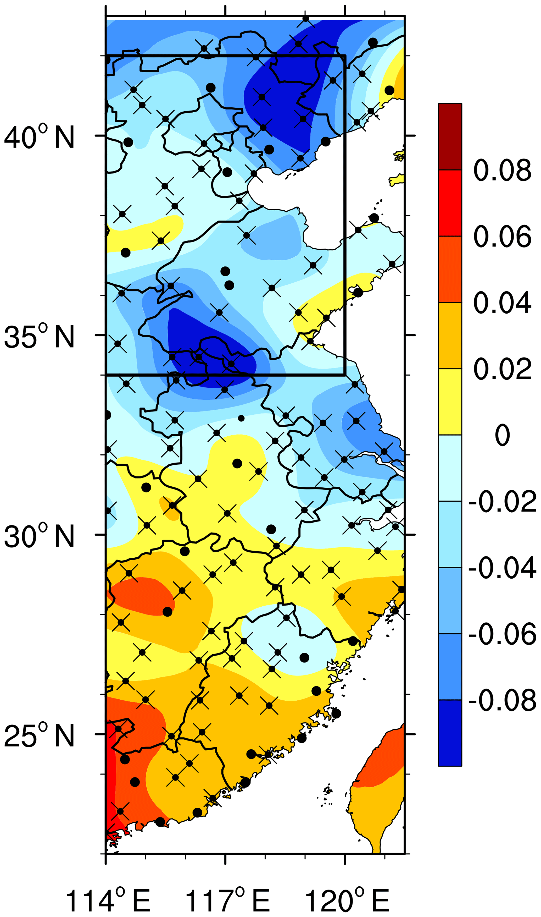
Figure 1The spatial pattern (shading) of the first EOF mode (variation contribution: 33 %) for HDJ from 1979 to 2015. The black crosses and dots represent the locations of the observation stations. The cross (dot) indicates that the HDJ accounted for more (less) than 70 % of the total winter haze days.

Figure 2The variation of (a) HDJNCP from 1979 to 2015 and (b) daily maximum PM2.5 from December to January in 2015 over the NCP area. The error bars in panel (a) represent 1 standard error among the measured sites.
The HDJNCP was stable during 1979 to 1992 and decreased from 1993 to 2009. After 2009, the HDJNCP showed a strong upward trend. The minimum HDJNCP occurred in 2010, which was 17.5 days. Afterwards, the HDJNCP increased dramatically and persistently, reaching a maximum (i.e., 42.7 days) in 2015. The mass concentration of PM2.5 is an important indicator of haze pollution. The daily maximum of area-mean PM2.5 in 2015 is shown in Fig. 2b and was above 100 µg m−3. The concentrations of PM2.5 were relatively lower in January 2016 than those in December but still exceeded the threshold of pollution in China (i.e., 75 µg m−3). On 23 December, the most disastrous haze occurred, and the area-mean PM2.5 concentration approached 500 µg m−3, indicating quite poor air quality and a serious health risk.
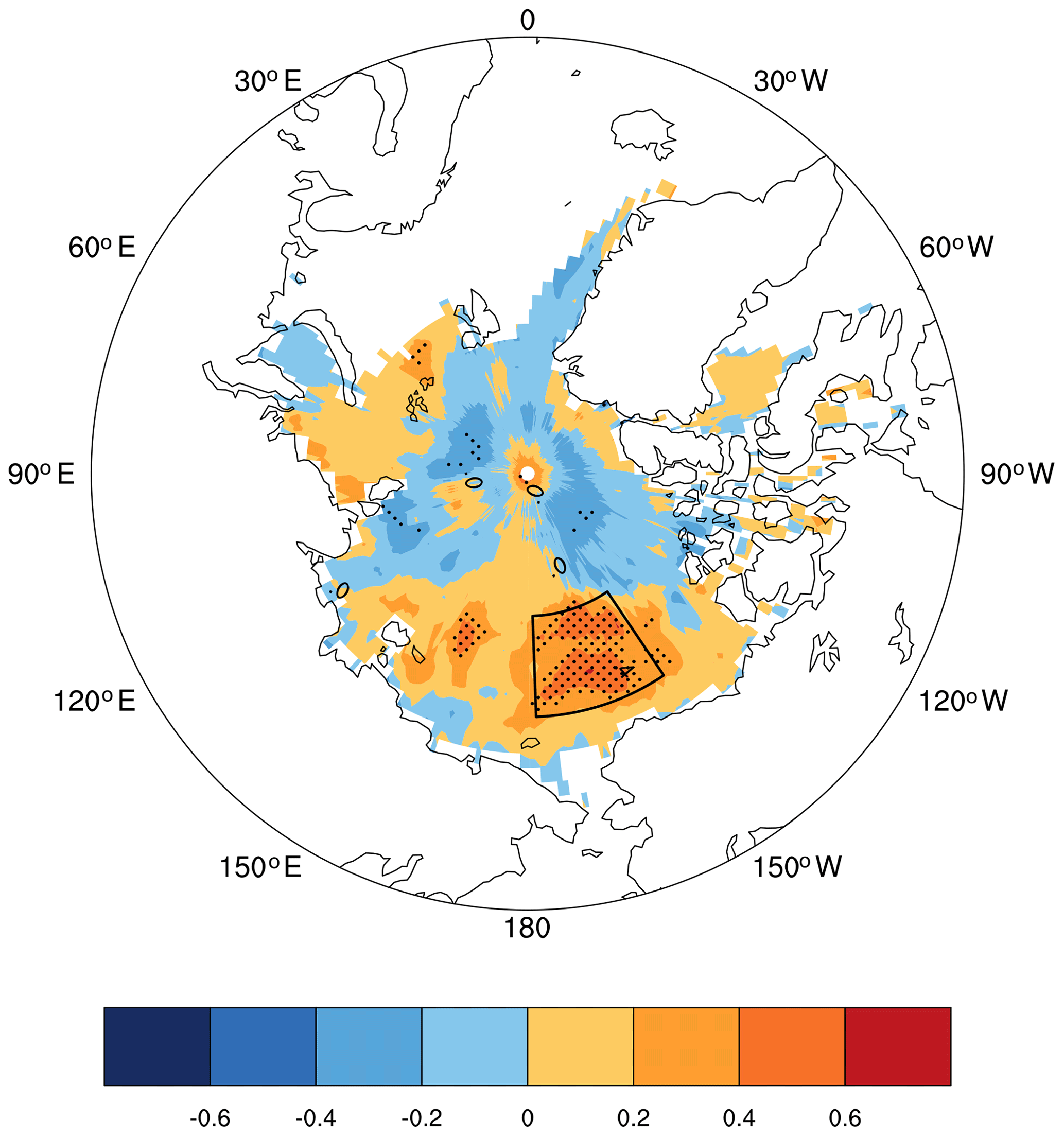
Figure 3The correlation coefficient (CC) between the HDJNCP and September–October sea ice concentration from 1979 to 2015, after detrending. The black dots indicate CCs exceeding the 95 % confidence level (t test). The black box represents the selected Beaufort Sea.
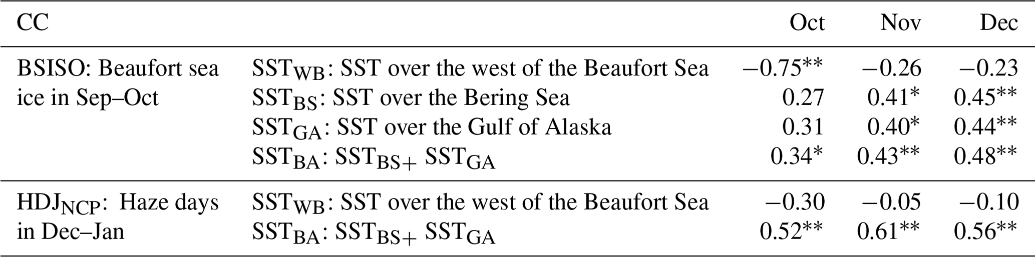
Table 1The correlation coefficient (CC) between the BSISO (HDJNCP) and SST indices in October, November and December. The linear trend was removed. The “*” indicates that the CCs exceed the 95 % confidence level, and “**” indicates that the CCs exceed the 99 % confidence level. The meanings of the abbreviations were also explained.
As illustrated by Wang et al. (2015), the autumn ASI significantly and negatively affected the haze pollution in the east of China by modulating the large-scale atmospheric circulations and local meteorological conditions. Furthermore, the opposite pattern of the number of haze days in the east of China was revealed in Fig. 1. To confirm the response of HDJNCP to the autumn sea ice, the correlation coefficients between the HDJNCP and the September–October sea ice were assessed after removing the linear trend (Fig. 3). A positive correlation was found from the East Siberian Sea to the Beaufort Sea. In this broad region, the significantly correlated area was intensively located over the west of the Beaufort Sea. Thus, the area-averaged September–October sea ice area over the west of the Beaufort Sea (73–80∘ N, 146–178∘ W) was calculated and denoted as the BSISO index, whose correlation coefficient with HDJNCP was 0.51 (above the 99 % confidence level) after removing the linear trend. This apparent positive relationship indicates that the efficient accumulation of the preceding autumn sea ice over the west of the Beaufort Sea significantly intensified the number of haze days in early winter over the NCP area. To confirm this connection, the year-to-year change of the sea ice concentration was examined (Fig. 4). From 1979 to 2015, there were 7 years with a significantly negative BSISO (i.e., BSISO < 0.8 × its standard deviation) and 10 years with a significantly positive BSISO (i.e., BSISO > 0.8 × its standard deviation). During 65 % of these years, the significant BSISO anomalies corresponded to HDJNCP anomalies with the same mathematical sign. There were no significantly opposite responses of HDJNCP (| HDJNCP | > 0.8 × its standard deviation) to the BSISO anomalies. Furthermore, the relationship seemed to be enhanced after the mid-1990s. The same mathematical signs of the anomalies appeared more frequently.

Figure 4Distributions of the September–October sea ice concentration after removal of the linear trend in typical years (i.e., the year when |BSISO| > 0.8× its standard deviation). The “+” and “−” represent the mathematical sign of the BSISO and HDJNCP indices. The “.sig” indicates that the absolute value of the index anomaly was larger than 0.8× its standard deviation.
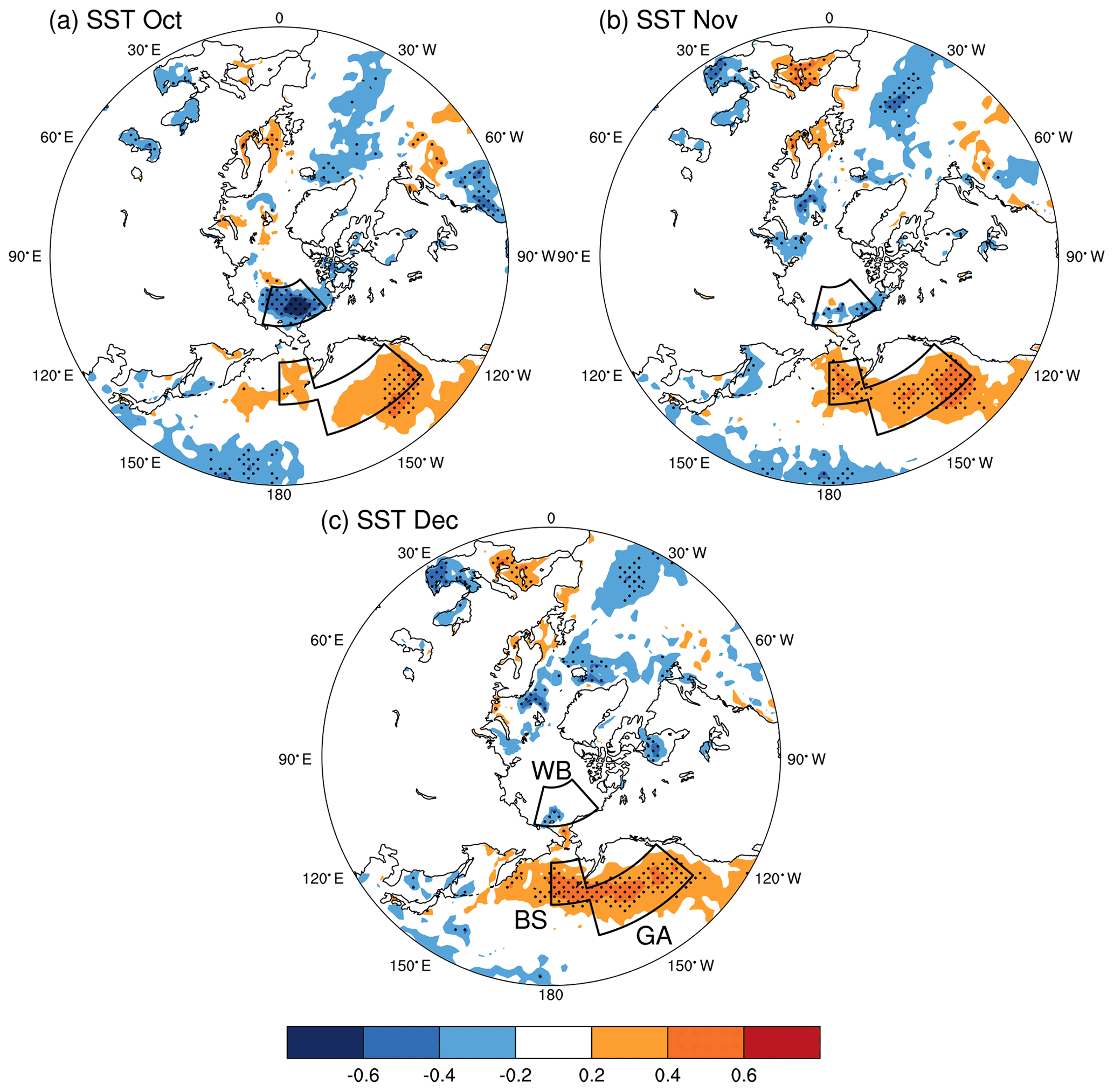
Figure 5The CC between the BSISO and SST in (a) October, (b) November and (c) December from 1979 to 2015, after detrending. The black dots indicate CCs exceeding the 95 % confidence level (t test). The black boxes (WB: west of Beaufort Sea, BS: Bering Sea and GA: Gulf of Alaska) are the significantly correlated areas, which were used to calculate the SST indices.
The positive sea ice anomalies, with high albedo, can efficiently reflect solar radiation and restore more fresh water, which could influence the local and adjacent SST. The correlation coefficients between BSISO and the simultaneous and subsequent SST were computed (Fig. 5). Because of efficient reflections of the solar radiation, the locally negative SST anomalies, located near the west of the Beaufort Sea (70–81∘ N, 166∘ E–138∘ W), were associated with the positive BSISO anomalies in October. In the following 2 months, these negative SST anomalies could not be sustained; i.e., these anomalous responses disappeared in November. However, the positive SST anomalies in the Bering Sea (49–60∘ N, 165–180∘ W) and the Gulf of Alaska (40–52∘ N, 130–165∘ W) appeared in October and were persistently enhanced in November and December. These three significantly correlated SSTs, located near the west of the Beaufort Sea (WB), over the Bering Sea (BS) and the Gulf of Alaska (GA), were defined as SSTWB, SSTBS and SSTGA, respectively. The correlation coefficients between these three indices were enumerated in Table 1 to present the change of the correlation with SST. Over time, the linkage between BSISO and local SST (i.e., SSTWB) rapidly receded. To confirm the role of the local SST on the HDJNCP, the correlation coefficient between HDJNCP and SSTWB was −0.30 in October (exceeding the 95 % confidence level) and −0.05 and −0.10 in the following November and December (insignificant). However, the correlation coefficients between the SSTBS (SSTGA) and BSISO were persistent and even became enhanced in November and December (Table 1). We speculated that the November SSTBS and SSTGA were the junction between the BSISO and HDJNCP.
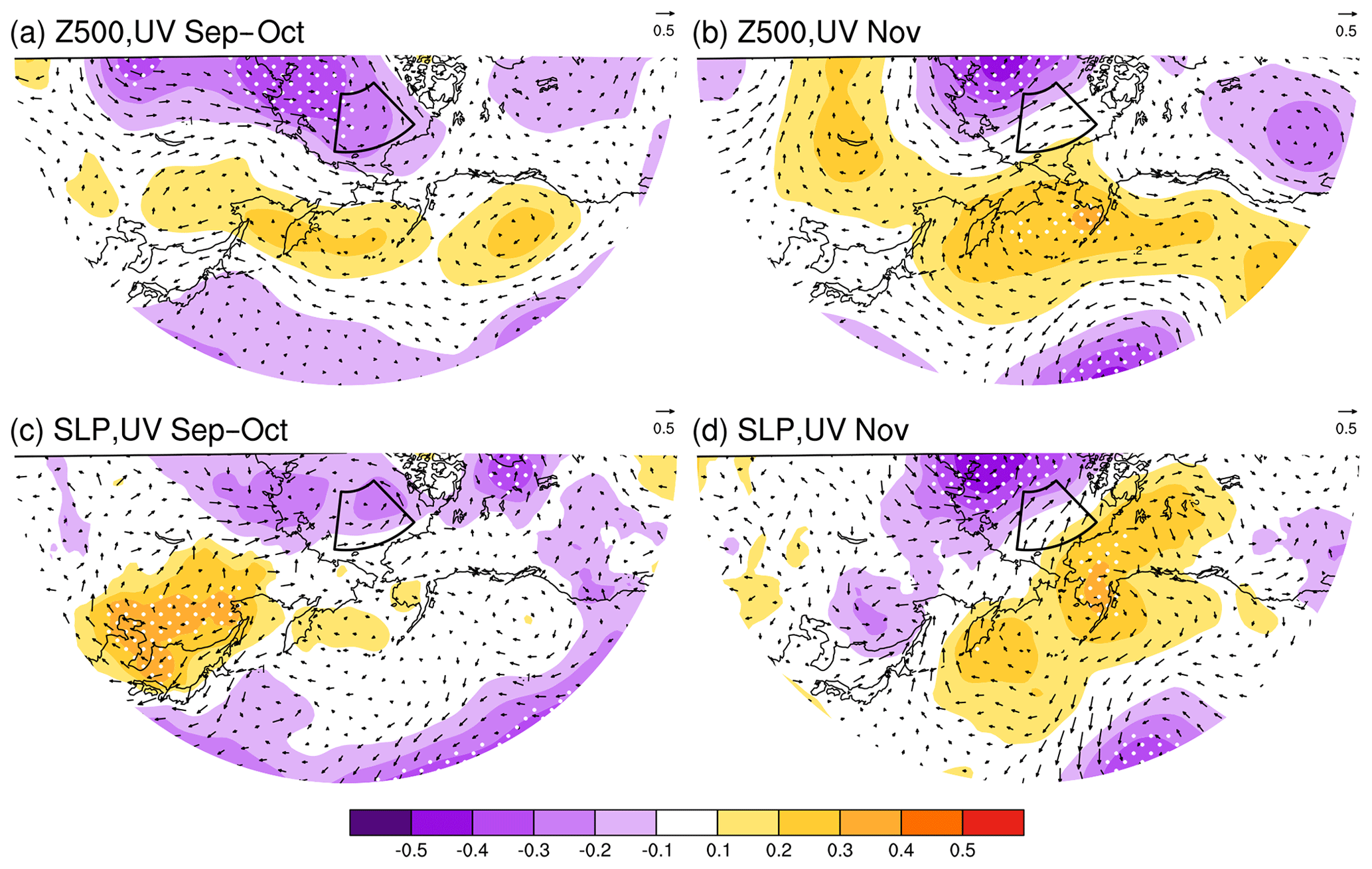
Figure 6The CC between BSISO and September–October (a) geopotential height (shading), wind (arrow) at 500 hPa, (c) SLP (shade) and surface wind (arrow) and between BSISO and November (b) geopotential height (shading), wind (arrow) at 500 hPa, (d) SLP (shade) and surface wind (arrow) from 1979 to 2015, after detrending. The white dots indicate CCs exceeding the 90 % confidence level (t test). The black box in panels (a)–(d) represents the location of the Beaufort Sea.
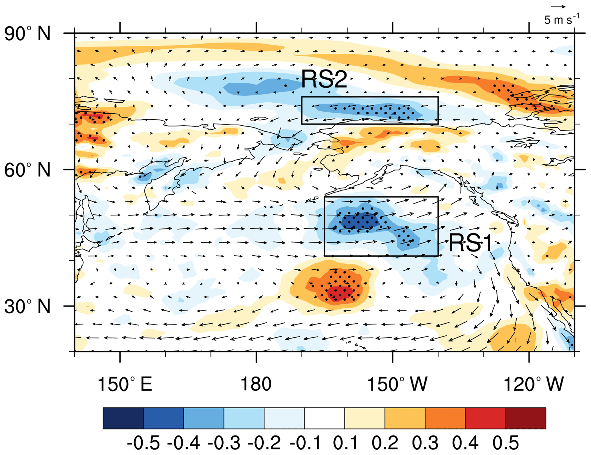
Figure 7The distribution of the climate mean surface wind (arrow) in November and the CC between the BSISO and surface wind speed in November from 1979 to 2015, after detrending. The black dots indicate CCs exceeding the 95 % confidence level (t test). The black boxes (RS1 and RS2) are the significantly correlated areas, which were used to calculate the WSPDRS1 and WSPDRS2 index.
According to the numerical results illustrated by Deser et al. (2007), the responses of atmospheric circulations to sea ice anomalies were initially baroclinic in the first 5–10 days and progressively became more barotropic and increased in both spatial extent and magnitude within 2 months. In September and October, due to the radiative cooling of the positive BSISO anomalies, the baroclinic responses of the atmospheric circulations manifested mainly as anomalous cyclonic circulations in the upper troposphere (Fig. 6a). There were also weak anticyclonic responses in the Bering Sea and Gulf of Alaska. In the subsequent November, the extent of these cyclonic and anticyclonic anomalies increased, especially the anticyclonic circulations over the Bering Sea and Gulf of Alaska (Fig. 6b). The barotropic structure of the atmospheric responses became more obvious; i.e., there were also cyclonic and anticyclonic circulations on both sides of the Beaufort Sea, near the surface (Fig. 6d). In addition, there were also positive SLP anomalies near the Aleutian Islands, indicating a weak Aleutian Low. Near the surface, a significant anomalous southerly existed between cyclonic and anticyclonic circulations, and an anomalous east wind existed in the south of the anticyclonic circulation (Fig. 6d). Overlapping with the climate mean state, the surface wind speeds over the RS1 (41–54∘ N, 140–165∘ W) and RS2 (70–76∘ N, 140–170∘ W) regions significantly receded (Fig. 7). The area-average surface wind speed was then calculated and denoted as WSPDRS1 and WSPDRS2 to examine its impacts on the simultaneous SST. In November, the climatological northeasterly through the Bering Strait transported cold seawater from the Arctic to the Bering Sea and resulted in a lower SST. The correlation coefficient between WSPDRS2 and SST is shown in Fig. 8 and was significantly negative in the Bering Sea. The driver of the cold seawater transportation, i.e., the surface wind, decreased and led to warmer SSTBS in November. Another reduction of surface wind speed, i.e., WSPDRS1, indicated the weakening of the west surface wind and accompanying subdued evaporation near the sea surface. This RS1 region was located consistently with the warmer Gulf of Alaska. The correlation coefficients between the WSPDRS1 and SSTGA were significantly negative, indicating that the reduction of WSPDRS1 resulted in a warmer sea surface over the Gulf of Alaska (Fig. 9a). Due to the weakening of the water evaporation, the latent heat release slowed down both in the Bering Sea and the Gulf of Alaska, which conserved more thermal energy on the sea surface (Fig. 9b). In addition, the upper anticyclonic circulations, with a clear sky, facilitated more shortwave solar radiation onto the sea surface. The absorbed and stored thermal energy, which was connected with the positive BSISO anomalies, heated the sea surface over the Gulf of Alaska in November, i.e., positive SSTGA anomalies. Both of the SSTGA and SSTBS were significantly influenced by the BSISO and synchronously changed. Thus, the SSTBS and SSTGA were integrated as SSTBA to analyze their corporate impacts on the HDJNCP. The variations of November SSTBA and the BSISO were strongly consistent, especially after 2000 (Fig. 10). As presented in Table 1, from October, the SSTBA began to significantly connect with the BSISO. Over time, this connection persisted and strengthened. The correlation coefficient between November (December) SSTBA and the BSISO was 0.43 (0.48), exceeding the 99 % significance test.
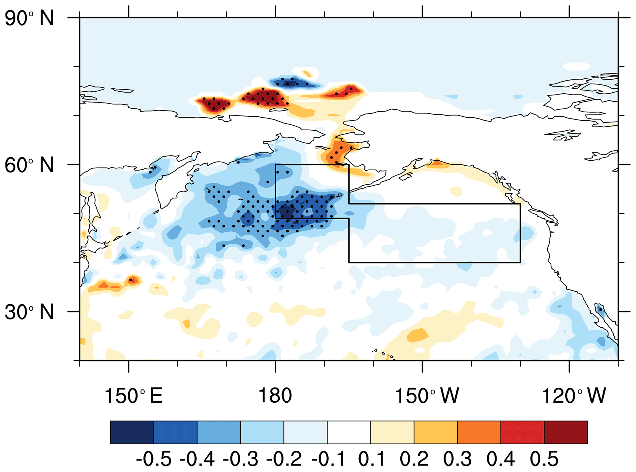
Figure 8The CC between WSPDRS2 and SST in November from 1979 to 2015. The black dots indicate that the CCs exceeded the 95 % confidence level (t test). The black box represents the BA (Bering Sea–Gulf of Alaska). The linear trend was removed.
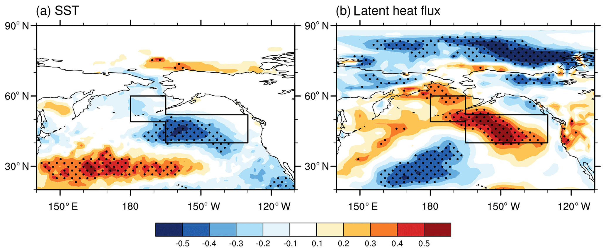
Figure 9The CC between WSPDRS1 and (a) SST and (b) latent heat flux in November from 1979 to 2015. The black dots indicate that the CCs exceeded the 95 % confidence level (t test). The black box represents the BA area. The linear trend was removed.
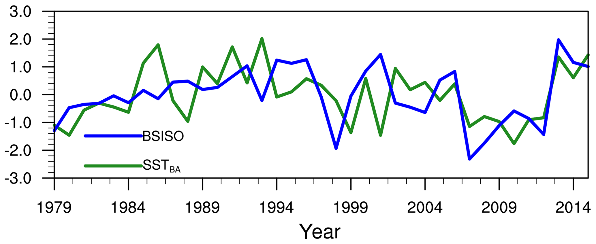
Figure 10The variation of the normalized BSISO (blue) and November SSTBA (green) from 1979 to 2015, after detrending.
Statistically, the November SSTBA was significantly correlated with the HDJNCP (i.e., the correlation coefficient was 0.61 and above the 99 % confidence level), showing strong impacts on the number of haze days in early winter over the NCP region. To reveal the physical processes, the associated atmospheric circulations and local meteorological conditions were diagnosed in Figs. 11–15. The warmer sea surface efficiently heated the above air and resulted in ascending motion from the Gulf of Alaska to the Aleutian Islands, which could extend to the atmosphere at 200 hPa (Fig. 11). Furthermore, significant accompanying descending motions at 200 hPa were stimulated from the Sea of Okhotsk to the Hawaiian Islands (Fig. 11a). Near the surface, there was also a sinking motion over the Hawaiian Islands (Fig. 11b). On the mid-troposphere, the significantly negative Z500 anomalies, i.e., cyclonic circulations, were exerted above the warmer Bering Sea and Gulf of Alaska (Fig. 12b). The responses of the December–January atmospheric circulations to the warmer November SSTBA showed deeply barotropic structures. There were also significant cyclonic circulations in the lower troposphere (Fig. 12c) and near the surface (Fig. 12d). At 500 hPa, there were significant anticyclonic anomalies located on both sides of the cyclonic circulations, i.e., over North China, the Sea of Japan, and the Cordillera Mountains. Thus, a Rossby wave-like train was induced by the SSTBA, which propagated from North China and the Sea of Japan, through the Bering Sea and Gulf of Alaska, to the Cordillera Mountains. This “+–+” pattern could also be recognized in the lower (Fig. 12c) and upper (Fig. 12a) troposphere. The anticyclonic circulations over North China and the Sea of Japan were recognized as the key atmospheric system to influence the haze pollution in the NCP area (Yin and Wang, 2016a; Yin et al., 2017). To confirm the linkage between this Rossby wave-like train and SSTBA, the area-averaged Z500 in three centers (30–50∘ N, 88–115∘ E; 45–60∘ N, 150∘ E–160∘ W; 50–60∘ N, 115–130∘ W) were calculated and are shown in Fig. 13. The correlation coefficients between the three centers, from west to east, with SSTBA were 0.47, −0.46 and 0.37, all above the 95 % confidence level. Due to the change of the pressure gradient, there were positive zonal westerlies from Lake Baikal to the Hawaiian Islands and negative westerly anomalies from eastern China to the west subtropical Pacific (Fig. 12a). Therefore, zonal west winds prevailed in the mid-high latitudes, and the meridionality of the atmosphere was reduced. The East Asia jet stream was weakened by anomalous easterlies and shifted northwards, indicating a decrease of the southward cold air activities. In addition, the southern section of the East Asian major trough, which reached the NCP area and guided cold air southward, was truncated by the anomalous anticyclonic circulations (Fig. 12b). In contrast, due to the cyclonic anomalies over the Aleutian area, the northern section of the East Asian major trough was enhanced but moved eastward. These large-scale anomalous atmospheric circulations could provide a suitable background for the enhancement of the potential of the haze weather (Yin and Wang, 2017a).
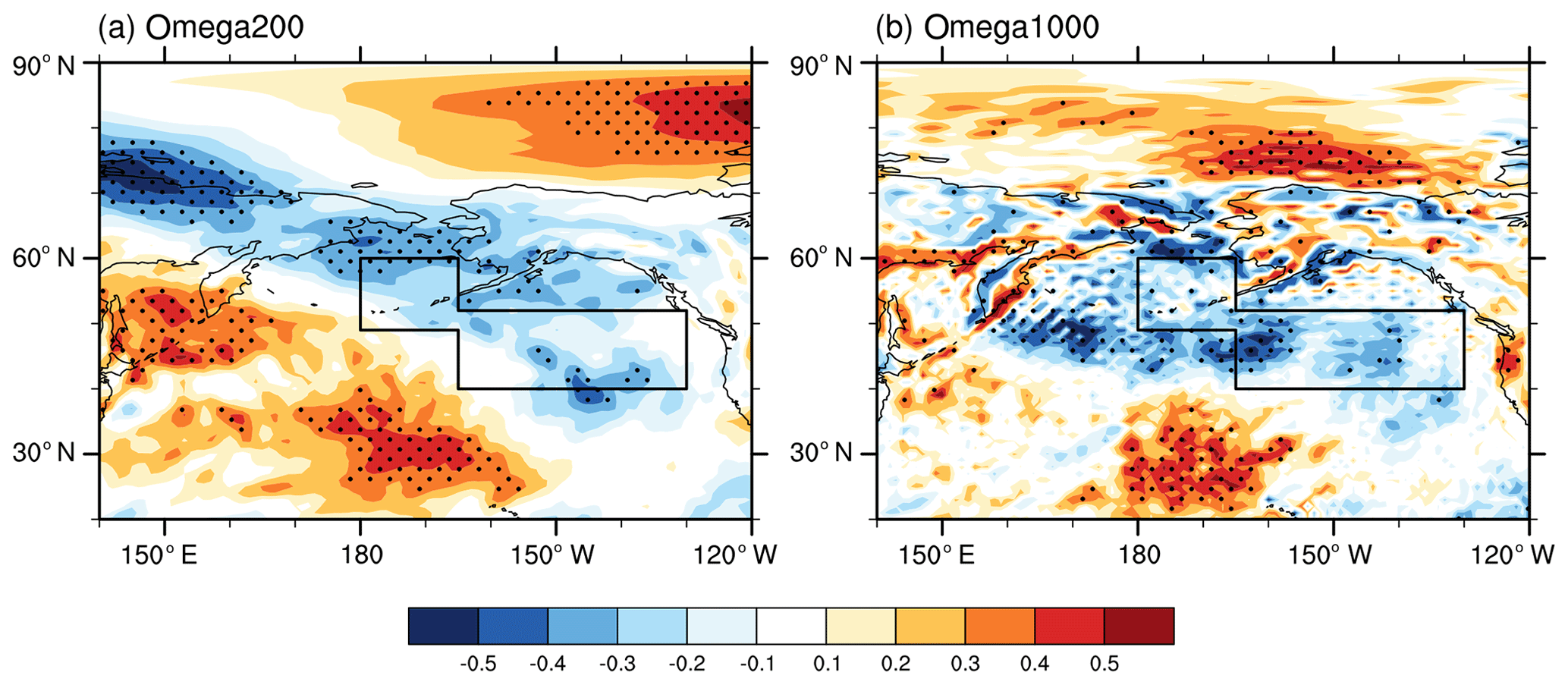
Figure 11The CC between November SSTBA and (a) omega (vertical velocity) at 200 hPa and (b) at 1000 hPa in December and January from 1979 to 2015. The black dots indicate that the CCs exceeded the 95 % confidence level (t test). The linear trend was removed. The black box represents the BA area.
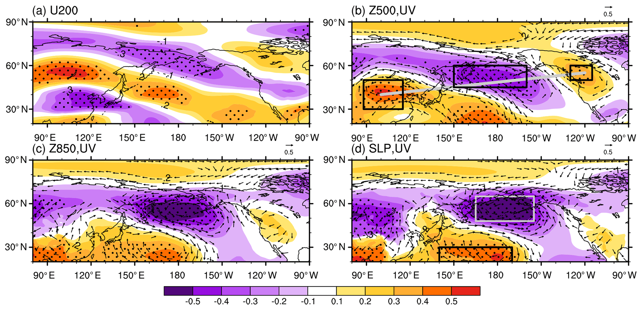
Figure 12The CC between the November SSTBA and (a) zonal wind at 200 hPa, (b) wind (arrow), geopotential height (shading) at 500 hPa, (c) wind (arrow), geopotential height (shading) at 850 hPa, (d) surface wind (arrow) and SLP (shading) in December–January from 1979 to 2015. The black dots indicate that the CCs exceeded the 95 % confidence level (t test). The linear trend was removed. The black boxes in panel (b) represent the three anomalous centers at 500 hPa, and the gray and black boxes in panel (d) represent the negative and positive anomalous centers.
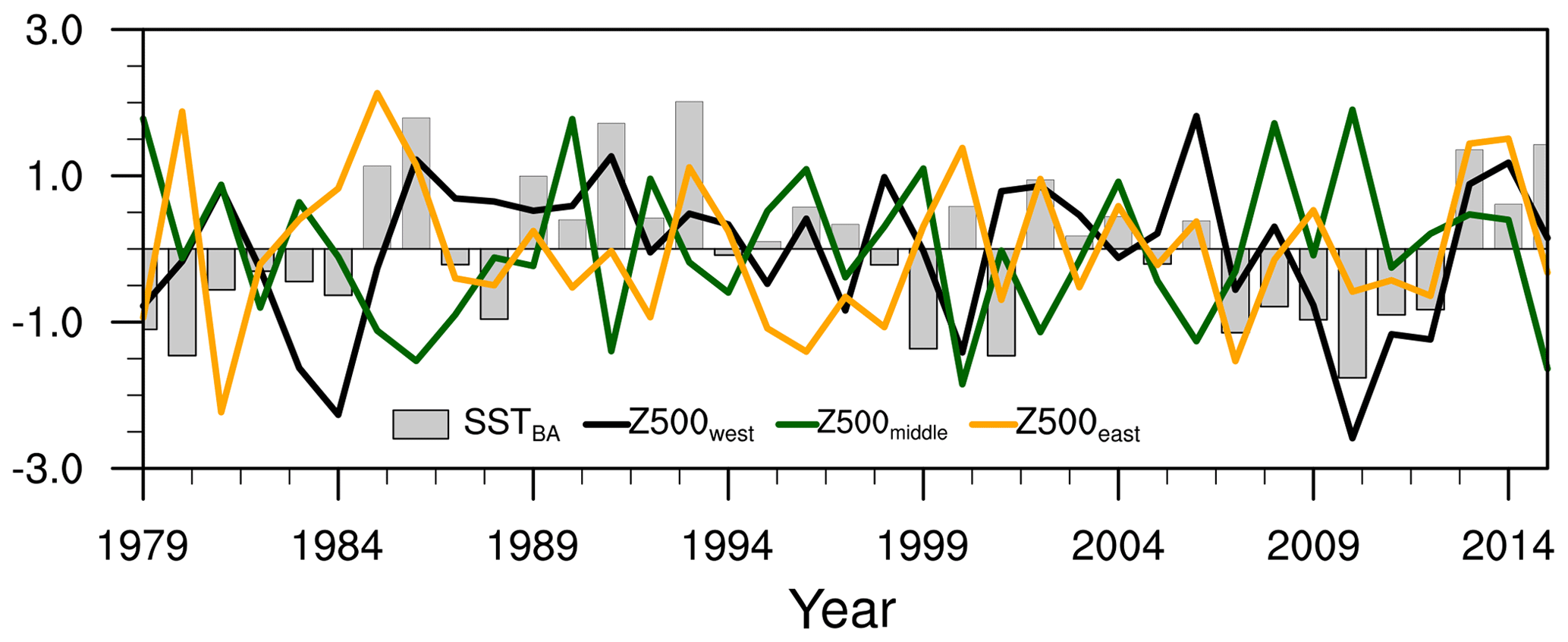
Figure 13The variation of the November normalized SSTBA (gray bar) and area-averaged geopotential height at 500 hPa of the three anomalous centers (west: black, middle: green, east: orange) from 1979 to 2015, after detrending.
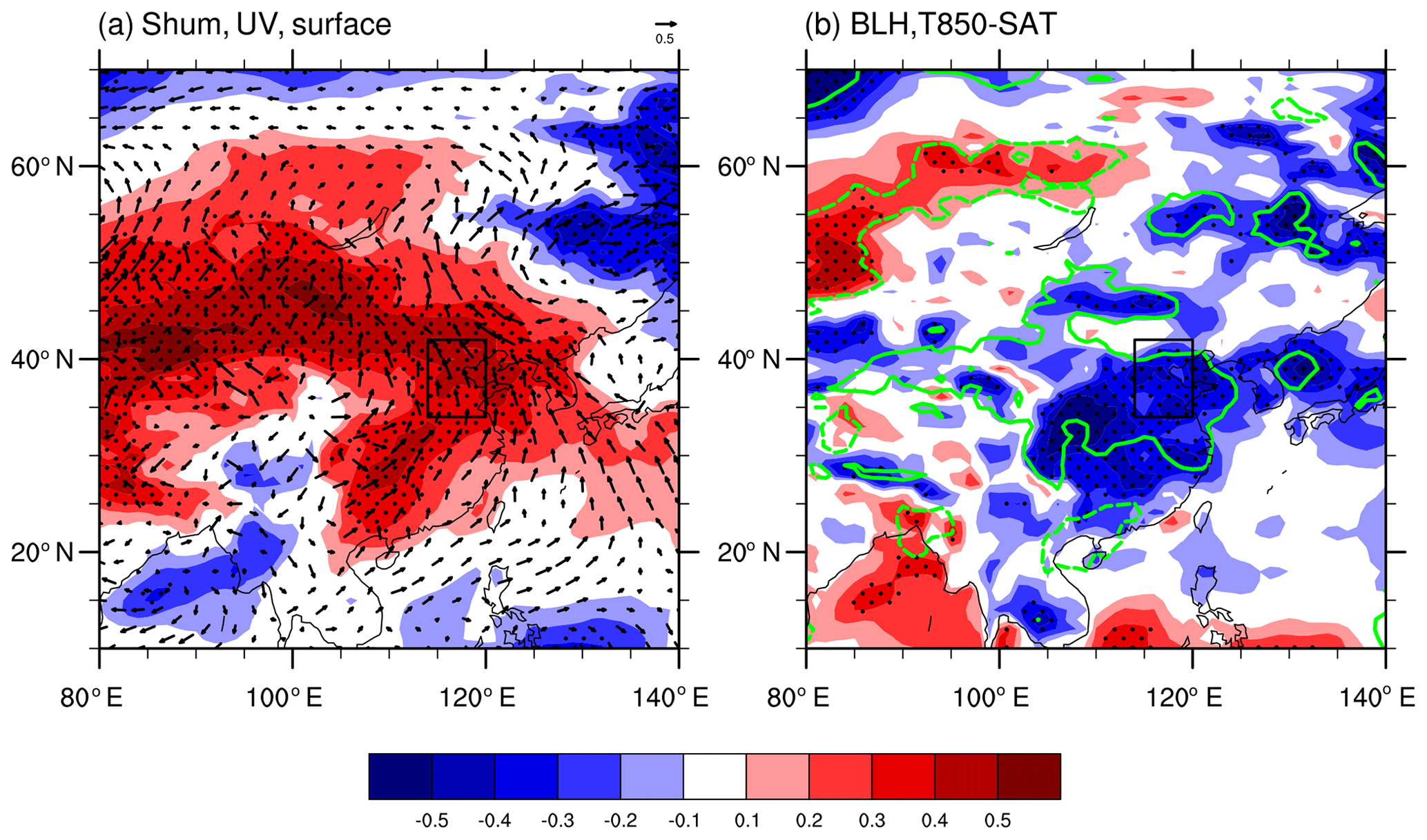
Figure 14The CC between the November SSTBA and (a) surface wind (arrow), specific humidity (Shum, shading) at 1000 hPa, (b) BLH (shading) and thermal inversion potential (contour) from 1979 to 2015. The black dots indicate that the CCs exceeded the 90 % confidence level, and the solid (dashed) green lines indicate that the positive (negative) correlations exceeded the 90 % confidence level (t tests). The linear trend was removed. The black boxes represent the NCP area. The thermal inversion potential was defined as the air temperature at 850 hPa minus SAT.
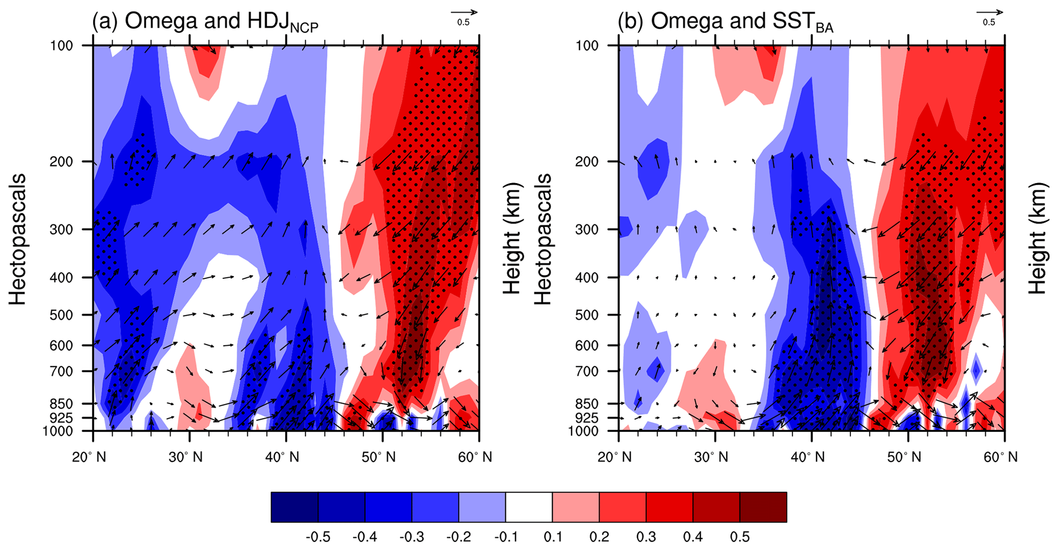
Figure 15The cross section (114–120∘ E mean) CC of (a) the HDJNCP and (b) November SSTBA for omega (shading) and wind (arrow) in December–January from 1979 to 2015. The black dots indicate that the CCs exceeded the 95 % confidence level (t test). The linear trend was removed.
Near the surface, because of the SSTBA heating, the Aleutian Low moved eastward and was enhanced over the Bering Sea and Gulf of Alaska. Consistent with the barotropic anomalies in the above air, there were positive SLP anomalies from Northeast China to the West Pacific (Fig. 12d). That is, a north–south seesaw over the North Pacific was discerned clearly, similar to the anomalous North Pacific Oscillation (NPO) pattern (Rogers, 1981). The difference of SLP (20–30∘ N, 140∘ E–170∘ W minus 48–65∘ N, 165∘ E–155∘ W) was calculated to quantify this seesaw pattern, whose correlation coefficients with the BSISO, SSTBA and HDJNCP were 0.33, 0.64 and 0.61, respectively. Bounded by the east of China, the south positive center of NPO and the negative anomalies occupied the West Pacific and Eurasia, respectively. The drivers of the East Asian winter monsoon, i.e., the pressure gradient between the continent and the ocean, became weak, indicating the limitation of cold air and ventilation conditions. Compared to the local zonal wind, the meridional wind played more important roles on weakening the horizontal dissipation conditions of the air. The southerly anomalies were located over the coastal area of China and transported moisture to the NCP area (Fig. 14a), providing moist air for haze formation. In winter, the anomalous south winds also weakened the prevailing northerlies and reduced the invasion of cold air. The humid atmosphere was conducive to the hygroscopic growth of pollutant particles, which reduced the visibility rapidly and structured stable weather conditions. The surface wind speed, indicating the horizontal dispersion capacity of the atmosphere, also subsided. In addition, the shallow thermal inversion layer or the boundary layer limited the upward dispersion of the pollutant particles. As shown in Fig. 14b, the intensity of the thermal inversion over the NCP area was significantly heightened while the boundary layer significantly declined. Generally, the air on the high altitude was relatively dry and clean. The sinking of the upper air to the surface was an important approach in dispersing the surface pollution (Sun et al., 2017). Instead, the upward motion above the boundary layer resisted the breaking of the thermal layer and was in favor of haze occurrence (Fig. 15a). The associated anomalous descending flow was blocked in the north of 46∘ N, which was consistent with the location of the northward cold air activities (Fig. 15a). Influenced by the warmer SSTBA, there were anomalous ascending motions over the NCP area. Thus, the weakened downward transportation of momentum was not sufficient to enhance the winds near the surface and break the thermal inversion layer. Therefore, the clear, dry and cold air was difficult to transport to the surface, indicating the failure of the blowing wind. Under poor ventilation conditions, i.e., the horizontal and vertical dispersion was limited, the fine particles were apt to accumulate and cause haze pollution. Combined with favorable moisture conditions, the haze exacerbated rapidly and perniciously.
The connection between the haze pollution in North China and ASI and associated physical mechanisms were statistically analyzed in the above sections. To confirm the causality, numerical experiments were designed with the public CESM-LE datasets. To be consistent with the observational results, the variables from CESM-LE from 1979 to 2015 are employed, which were combined by the historical simulation during 1979–2005 and the data during 2006–2015 from the Representative Concentration Pathway 8.5 forcing simulation. A total of 35 CESM-LE ensemble members were used here. The CESM-LE simulations were completed by the fully coupled CESM model; thus the interactions among sea ice, sea temperature and atmosphere can be contained. The years when the sea ice anomalies concentrated in the west of the Beaufort Sea were selected, and the differences between the positive BSISO and negative BSISO years were be identified as the responses to the sea ice anomalies. In the numerical experiment, all available CESM-LE members were included and different amplitudes of sea ice anomalies were composited; thus the uncertainty from the internal variability were largely reduced.
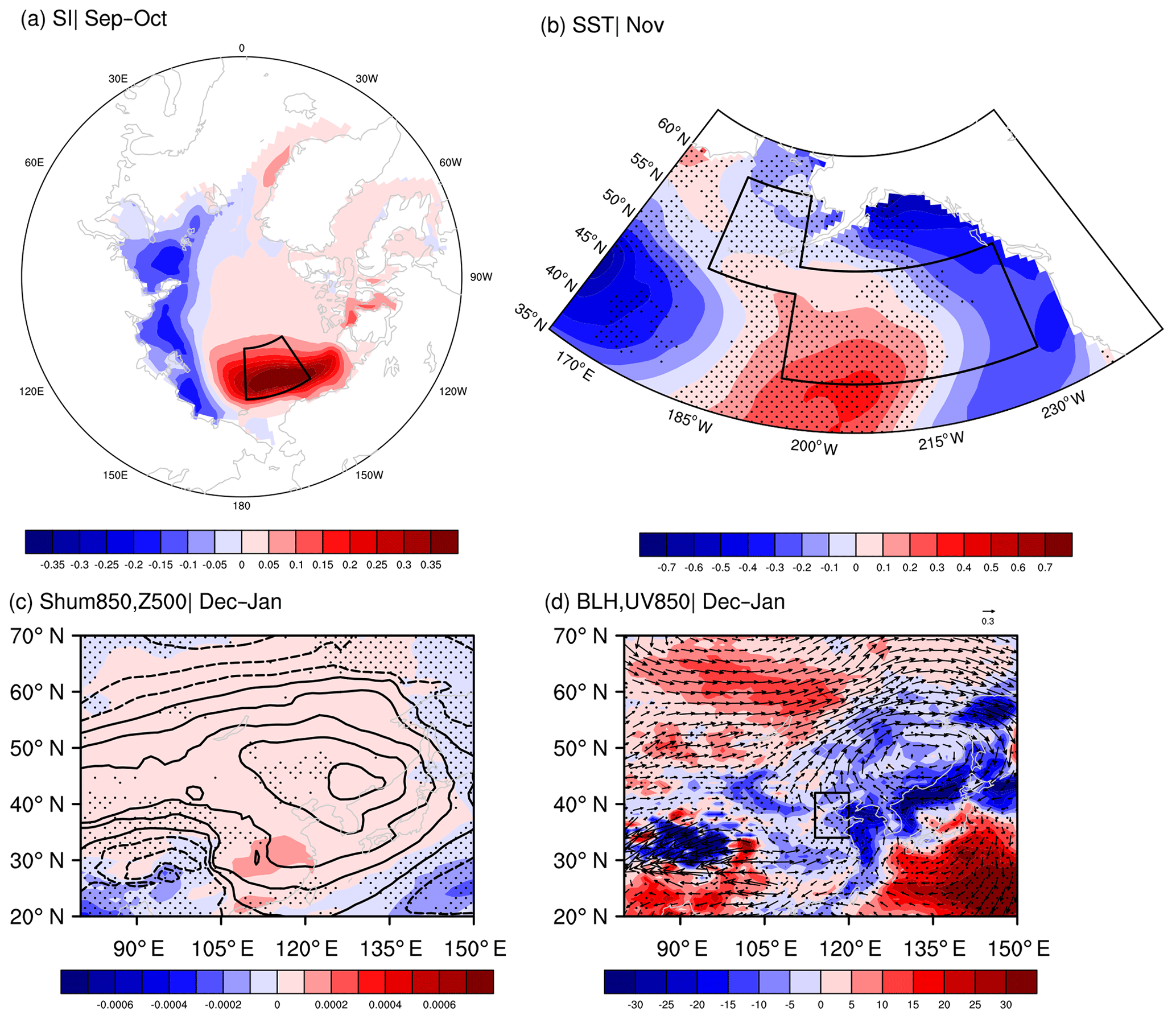
Figure 16Composite difference of (a) September–October sea ice concentration, (b) sea surface temperature in November, (c) geopotential height (contour) at 500 hPa, surface specific humidity in December–January, (d) BLH (shading) and surface wind (arrow) in December–January. The black box in panel (a) represents the location of the Beaufort Sea, and in panel (b) it represents the BA area. Results are based on 35 ensembles of CESM-LE simulations. The black dots indicate that the mathematical sign of the changes with shading from more than 50 % of the members are consistent with the ensemble mean.
In Fig. 16a, the sea ice anomalies were obvious in the key region. The maximum of the difference in sea ice concentration was more than 35 % (Fig. 16a). In the following November, the accumulated sea ice favored increased SST over the Gulf of Alaska (Fig. 16b), which is in good accordance with the observed results. Although there were weaker but negative SST responses in the Bering Sea, the positive SST anomalies extended southwards and enhanced the air–sea interaction. In terms of the corresponding atmospheric circulations with regard to anomalous BSISO, the composite difference was also consistent with the observed results. The anticyclonic anomalies of the geopotential height at 500 hPa were also well reproduced by the numerical model in the early winter (Fig. 16c). In the lower troposphere, there were also anomalous anticyclones over North China and Northeast China, which induced anomalous southerlies (Fig. 16d) and weakened the cold air from the high latitudes. Furthermore, the moist air condition (Fig. 16c) and lower boundary layer (Fig. 16d) were also verified to be significantly connected with the positive BSISO anomalies. Consistent with the observed results, the linkages between the BSISO and the haze pollution in the North China also exist in CESM-LE simulations. Meanwhile, the corresponding physical mechanisms were also well reproduced by the large ensemble members. The performances of numerical models in the mid-high latitudes were consistently limited; however, the results from CESM-LE here successfully captured major features and general physical processes as expected. Consequently, the robustness of the proposed connections and physical mechanisms were strongly confirmed.
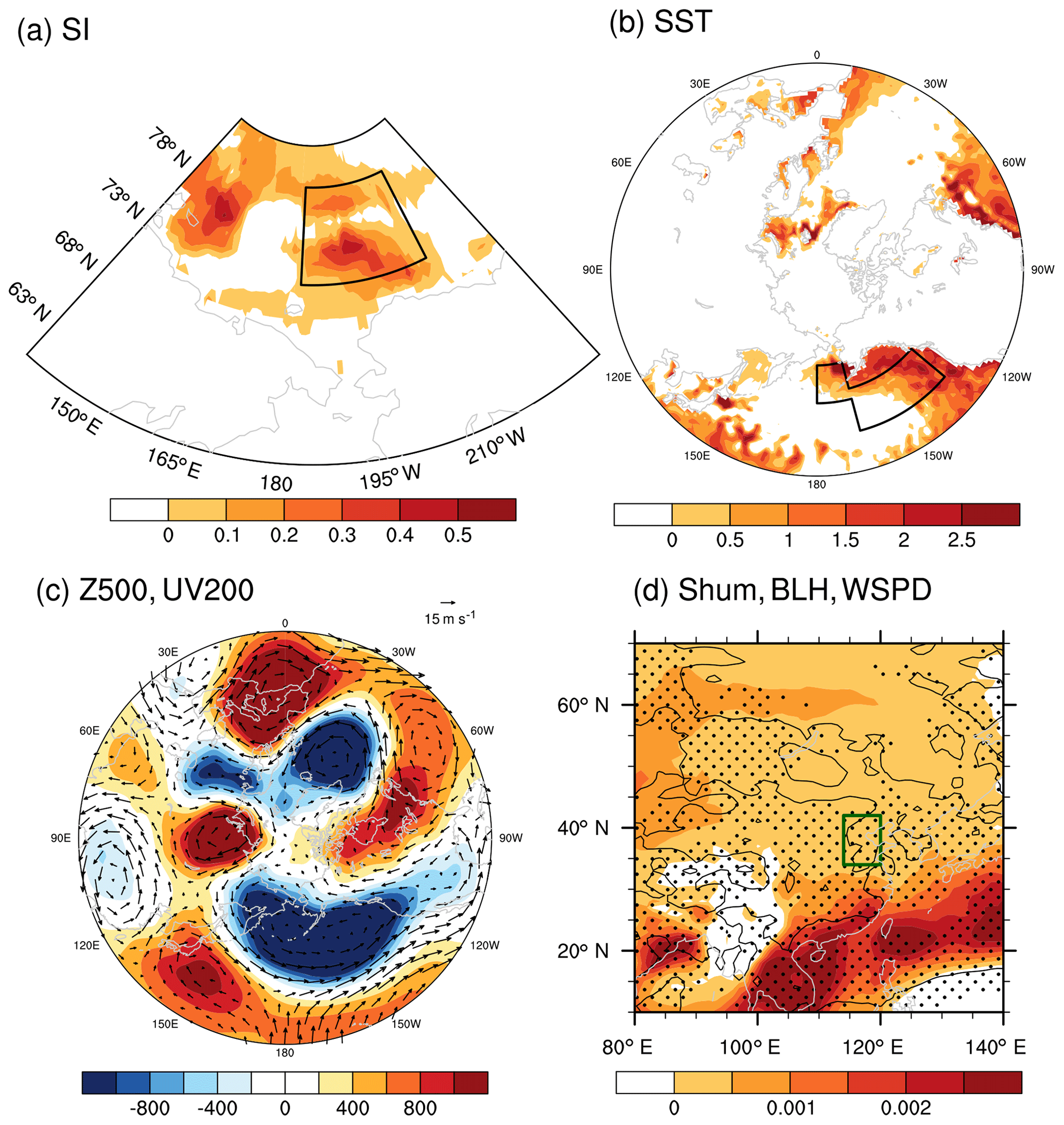
Figure 17The distributions of (a) September–October sea ice concentration in 2015, (b) sea surface temperature in November 2015, (c) geopotential height (shading) at 500 hPa, wind (arrow) at 200 hPa in December–January 2015, (d) specific humidity (shading) at 1000 hPa, BLH (black dots indicate that its value is negative) and WSPD (contour, solid black lines indicate a negative value) in December–January 2015. The black box in panel (a) represents the location of the Beaufort Sea, and in panel (b) it represents the BA area. The linear trend was removed.
In the subseasonal scale, the haze weather in early winter occurred more frequently and varied differently from that in February. In this study, the close relationship between the number of haze days in early winter in the NCP area and the September–October sea ice in the west of the Beaufort Sea, with a correlation coefficient of 0.51, was revealed. The positive September–October sea ice anomalies over the west of the Beaufort Sea strongly intensified the early winter haze pollution over the NCP area, or more precisely, increased the number of haze days. Associated physical mechanisms were further examined. Due to the high albedo and efficient reflections, the local SST in October became cooler than the climate mean state, showing the radiative cooling effect. The responses of the atmospheric circulations initially manifested as anomalous cyclonic circulations in the upper troposphere and then developed into cyclonic and anticyclonic circulations on both sides of the Beaufort Sea in the subsequent November. The decreased surface wind through the Bering Strait could not transport cold seawater to the Bering Sea as usual and led to a warmer sea surface over the Bering Sea. The reduction of surface wind speed over the Gulf of Alaska weakened the seawater evaporation and the latent heat release, which conserved more thermal energy in the sea surface, i.e., positive SST anomalies.
The November SST anomalies over the Bering Sea and Gulf of Alaska acted as a bridge in the close relationship between the BSISO (R=0.43, exceeding the 99 % confidence level) and HDJNCP (R=0.61). The warmer sea surface efficiently heated the air above and resulted in significant responses in the atmosphere. In the upper troposphere, zonal west wind anomalies prevailed in the mid-high latitudes, and the meridionality of the atmosphere was reduced, indicating the decrease of the southward cold air activities. A +–+ Rossby wave-like train propagated from North China and the Sea of Japan, through the Bering Sea and Gulf of Alaska, to the Cordillera Mountains. Near the surface, the NPO-like pattern and the negative SLP anomalies over Eurasia induced southerly anomalies over the coastal area of China, providing a calm and moist environment for haze formation. In addition, the intensity of the thermal inversion over the NCP area was significantly enhanced, and the clear, dry and cold air was difficult to transport to the surface. The horizontal and vertical dispersions were both limited, so the fine particles were apt to accumulate and cause haze pollution. The linkages and corresponding physical mechanisms were well reproduced via the large CESM-LE ensembles, confirming the causality.
In this study, the response of the number of haze days in early winter in the North China Plain to the autumn Beaufort sea ice and the associated physical mechanisms were investigated. As shown in Fig. 2, the HDJNCP was 42.7 days and reached its maximum in 2015. Thus, the measurements in 2015 were composited after removing the linear trend to verify the results from the observational analyses (Fig. 17). In September–October 2015, there were positive sea ice anomalies on the west of the Beaufort Sea (Fig. 17a), which satisfied the close relationship revealed in this study. Meanwhile, an obviously warmer SST in November was observed in most of the BA region (Fig. 17b), transferring the impacts of the BSISO. As a result, a weaker East Asia jet stream, an anomalous southerly (Fig. 17c), limited horizontal and vertical dispersion conditions, and moist air (Fig. 17d) enhanced the early winter haze pollution in 2015. However, some questions remain unanswered and should be investigated with numerical models in future work. For example, the internal dynamic and thermal processes and how the positive sea ice anomalies (radiative cooling) affected the atmospheric circulations are not fully understood. During this work, linear correlation analyses were the main research technique, and a linear relationship was discovered. In fact, the dynamic–thermodynamic processes in the air–ice interaction are neither straightforward nor necessarily linear (Zhang et al., 2000; Gao et al., 2015). Considering the contradiction among the results by a single numerical model (Gao et al., 2015), a multi-model ensemble was required to solve the internal physical mechanisms. Furthermore, the November SST anomalies over the Bering Sea and Gulf of Alaska were treated as a bridge to connect the sea ice and the haze pollution. It is necessary to examine whether this bridge was constructed all the time. Particularly, after 2010, haze pollution became more serious. The driven role of the BSISO and the bridge of SSTBA needs to be verified. Moreover, as revealed by the EOF decomposition, the number of haze days in southern China varied differently. Its relationship with the sea ice in the Arctic is still unclear and needs to be addressed. The significant relationship revealed in this study and associated previous work potentially improved the monthly prediction of haze pollution. Valuable haze predictions are urgently needed by the scientific decision-making departments to control haze pollution in China (Wang, 2018).
Sea ice concentration data can be downloaded from the Met Office Hadley Centre: https://www.metoffice.gov.uk/hadobs/hadisst/data/download.html (Met Office Hadley Centre, 2018). The ground observations are from the website: http://data.cma.cn/ (CMA, 2018). The atmospheric composition data can be obtained from the authors. Atmospheric data and land surface data are available on the ERA-Interim website: http://www.ecmwf.int/en/research/climate-reanalysis/era-interim (ERA-Interim, 2018). The monthly heat flux data are available from the NCEP/NCAR data archive: http://www.esrl.noaa.gov/psd/data/gridded/data.ncep.reanalysis.html (NCEP/NCAR, 2018). The simulation data are available from the Community Earth System Model Large Ensemble datasets (2018): http://www.cesm.ucar.edu/projects/community-projects/LENS/data-sets.html.
ZY and HW thought of the idea, ZY and YL created the figures, and ZY wrote the manuscript.
The authors declare that they have no conflict of interest.
This research was supported by the National Natural Science Foundation of
China (41705058 and 91744311), the National Key Research and Development
Plan (2016YFA0600703), the CAS–PKU Partnership program, and the funding of
the Jiangsu Innovation and Entrepreneurship team.
Edited by: Jianping Huang
Reviewed by: two anonymous referees
Cai, W. J., Li, K., Liao, H., Wang, H. J., and Wu, L. X.: Weather Conditions Conducive to Beijing Severe Haze More Frequent under Climate Change, Nat. Clim. Change, 7, 257–262, https://doi.org/10.1038/nclimate3249, 2017.
Chen, H. P. and Wang, H. J.: Haze Days in North China and the associated atmospheric circulations based on daily visibility data from 1960 to 2012, J. Geophys. Res., 120, 5895–5909, https://doi.org/10.1002/2015JD023225, 2015.
Chen, H., Wang, H., Sun, J., Xu, Y., and Yin, Z.: Anthropogenic fine particulate matter pollution will be exacerbated in eastern China due to 21st century GHG warming, Atmos. Chem. Phys., 19, 233–243, https://doi.org/10.5194/acp-19-233-2019, 2019.
CMA: Ground observations, available at: http://data.cma.cn/, last access: 3 April 2018.
Cohen, J. L., Furtado, J. C., Barlow, M. A., Alexeev, V. A., and Cherry, J. E.: Arctic warming, increasing snow cover and widespread boreal winter cooling, Environ. Res. Lett., 7, 014007, https://doi.org/10.1088/1748-9326/7/1/014007, 2012.
Community Earth System Model Large Ensemble datasets: http://www.cesm.ucar.edu/projects/community-projects/LENS/data-sets.html, last access: 14 December 2018.
Dee, D. P., Uppala, S. M., Simmons, A. J., Berrisford, P., Poli, P., Kobayashi, S., Andrae, U., Balmaseda, M. A., Balsamo, G., Bauer, P., Bechtold, P., and Beljaars, A. C. M.: The ERA-Interim reanalysis: configuration and performance of the data assimilation system, Q. J. Roy. Meteor. Soc., 137, 553–597, https://doi.org/10.1002/qj.828, 2011.
Deser, C., Tomas, R. A., and Peng, S.: The transient atmospheric circulation response to north atlantic sst and sea ice anomalies, J. Climate, 20, 4751, https://doi.org/10.1175/JCLI4278.1, 2007.
Ding, Y. H. and Liu, Y. J.: Analysis of long-term variations of fog and haze in China in recent 50 years and their relations with atmospheric humidity, Sci. China Ser. D: Earth Sci., 57, 36–46, 2014 (in Chinese).
ERA-Interim: Atmospheric data, available at: http://www.ecmwf.int/en/research/climate-reanalysis/era-interim, last access: 7 May 2018.
Fan, K., Xie, Z. M., Wang, H. J., Xu, Z. Q., and Liu, J. P.: Frequency of spring dust weather in North China linked to sea ice variability in the Barents Sea, Clim. Dynam., 51, 4439, https://doi.org/10.1007/s00382-016-3515-7, 2017.
Gao, Y. and Chen, D.: A dark October in Beijing 2016, Atmos. Oceanic Sci. Lett., 10, 206–213, 2017.
Gao, Y. Q., Sun, J. Q., Li, F., He, S. P., Sandven, S., Yan, Q., Zhang, Z. S., Lohmann, K., Keenlyside, N., Furevik, T., and Sou, L. L.: Arctic Sea Ice and Eurasian Climate: A Review, Adv. Atmos. Sci., 32, 92–114, https://doi.org/10.1007/s00376-014-0009-6, 2015.
He, C., Liu, R., Wang, X. M., Liu, S. C., Zhou, T. J., and Liao, W. H.: How does El Niño-Southern Oscillation modulate the interannual variability of winter haze days over eastern China?, Sci. Total Environ., 651, 1892–1902, https://doi.org/10.1016/j.scitotenv.2018.10.100, 2019.
He, S. P.: Asymmetry in the Arctic Oscillation Teleconnection with January Cold Extremes in Northeast China, Atmos. Oceanic Sci. Lett., 8, 386–391, https://doi.org/10.3878/AOSL20150053, 2015.
Honda, M., Inoue, J., and Yamane, S.: Influence of low Arctic sea ice minima on anomalously cold Eurasian winters, Geophys. Res. Lett., 36, L08707, https://doi.org/10.1029/2008GL037079, 2009.
Kalnay, E., Kanamitsu, M., Kistler, R., Collins, W., Deaven, D., Gandin, L., Iredell, M., Saha, S., White, G., Woollen, J., Zhu, Y., Leetmaa, A., Reynolds, R., Chelliah, M., Ebisuzaki, W., Higgins, W., Janowiak, J., Mo, K. C., Ropelewski, C., Wang, J., Jenne, R., and Joseph, D.: The NCEP/NCAR 40-year reanalysis project, B. Am. Meteorol. Soc., 77, 437–471, https://doi.org/10.1175/1520-0477(1996)077<0437:TNYRP>2.0.CO;2, 1996.
Kay, J. E., Deser, C., Phillips, A., Mai, A., Hannay, C., Strand, G., Arblaster, J., Bates, S., Danabasoglu, G., Edwards, J., Holland, M., Kushner, P., Lamarque, J.-F., Lawrence, D., Lindsay, K., Middleton, A., Munoz, E., Neale, R., Oleson, K., Polvani, L., and Vertenstein, M.: The Community Earth System Model (CESM) Large Ensemble Project: A community resource for studying climate change in the presence of internal climate variability, B. Am. Meteorol. Soc., 96, 1333–1349, https://doi.org/10.1175/BAMS-D-13-00255.1, 2015.
Kim, B. M., Son, S. W., Min, S. K., Jeong, J. H., Kim, S. J., Zhang, X. D., Shim, T., and Yoon, J. H.: Weakening of the stratospheric polar vortex by Arctic sea-ice loss, Nat. Commun., 5, 4646, https://doi.org/10.1038/ncomms5646, 2014.
Li, F. and Wang, H. J.: Autumn sea ice cover, winter northern hemisphere annular mode, and winter precipitation in Eurasia, J. Climate, 26, 3968–3981, 2012.
Li, F. and Wang, H. J.: Relationship between Bering sea ice cover and East Asian winter monsoon Year-to-Year Variations, Adv. Atmos. Sci., 30, 48–56, 2013.
Li, F. and Wang, H. J.: Autumn Eurasian snow depth, autumn Arctic sea ice cover and East Asian winter monsoon, Int. J. Climatol., 34, 3616–3625, https://doi.org/10.1002/joc.3936, 2014.
Li, F., Wang, H. J., and Gao, Y. Q.: On the strengthened relationship between East Asian winter monsoon and Arctic Oscillation: A comparison of 1950–1970 and 1983–2012, J. Climate, 27, 5075–5091, https://doi.org/10.1175/JCLI-D-13-00335.1, 2014.
Li, F., Wang, H. J., and Gao, Y. Q.: Change in Sea Ice Cover is Responsible for Non-Uniform Variation in Winter Temperature over East Asia, Atmos. Oceanic Sci. Lett., 8, 376–382, https://doi.org/10.3878/AOSL20150039, 2015.
Li, K., Liao, H., Cai, W., and Yang, Y.: Attribution of anthropogenic influence on atmospheric patterns conducive to recent most severe haze over eastern China, Geophys. Res. Lett., 45, 2072–2081, https://doi.org/10.1002/2017GL076570, 2018.
Li, S. L., Han, Z., and Chen, H. P.: A Comparison of the Effects of Interannual Arctic Sea Ice Loss and ENSO on Winter Haze Days: Observational Analyses and AGCM Simulations, J. Meteor. Res., 31, 820–833, https://doi.org/10.1007/s13351-017-7017-2, 2017.
Liu, J. P., Zhang, Z. H., Horton, R. M., Wang, C. Y., and Ren, X. B.: Variability of North Pacific Sea Ice and East Asia North Pacific Winter Climate, J. Climate, 20, 1991–2001, https://doi.org/10.1175/JCLI4105.1, 2007.
Liu, J. P., Curry J. A., Wang, H. J., Song, M., and Horton, R. M.: Impact of declining Arctic sea ice on winter snowfall, P. Natl. Acad. Sci. USA, 109, 4074–4079, 2012.
Met Office Hadley Centre: Sea ice cover data, available at: https://www.metoffice.gov.uk/hadobs/hadisst/data/download.html, last access: 5 April 2018.
NCEP/NCAR: heat fluxes data, available at: http://www.esrl.noaa.gov/psd/data/gridded/data.ncep.reanalysis.html, last access: 10 April 2018.
Rayner, N. A., Parker, D. E., Horton, E. B., Folland, C. K., Alexander, L. V., Rowell, D. P., Kent, E. C., and Kaplan, A.: Global analyses of sea surface temperature, sea ice, and night marine air temperature since the late nineteenth century, J. Geophys. Res., 108, 4407, https://doi.org/10.1029/2002JD002670, 2003.
Rogers, J. C.: The North Pacific Oscillation, Int. J. Climatol., 1, 39–57, https://doi.org/10.1002/joc.3370010106, 1981.
Sun, X. C., Han, Y. Q., Li, J., Kang, G. H., and Wang, B. M.: Analysis of the Influence of Vertical Movement on the Process of Fog and Haze with Air Pollution, Plateau Meteorology, 36, 1106–1114, 2017 (in Chinese).
Wang, H. J., Chen, H. P., and Liu J. P.: Arctic sea ice decline intensified haze pollution in eastern China, Atmos. Oceanic Sci. Lett., 8, 1–9, 2015.
Wang, H.-J. and Chen, H.-P.: Understanding the recent trend of haze pollution in eastern China: roles of climate change, Atmos. Chem. Phys., 16, 4205–4211, https://doi.org/10.5194/acp-16-4205-2016, 2016.
Wang, H. J.: On assessing haze attribution and control measures in China, Atmos. Oceanic Sci. Lett., 11, 120–122, https://doi.org/10.1080/16742834.2018.1409067, 2018.
Wang, S. Y. and Liu, J. P.: Delving into the relationship between autumn Arctic sea ice and central–eastern Eurasian winter climate, Atmos. Oceanic Sci. Lett., 9, 366–374, https://doi.org/10.1080/16742834.2016.1207482, 2016.
Xu, X. P., Li, F., He, S. P., and Wang, H. J.: Subseasonal reversal of East Asian surface temperature variability in winter 2014/15, Adv. Atmos. Sci., 35, 737–752, https://doi.org/10.1007/s00376-017-7059-5, 2018.
Yang, Y., Liao, H., and Lou, S.: Increase in winter haze over eastern China in recent decades: Roles of variations in meteorological parameters and anthropogenic emissions, J. Geophys. Res.-Atmos., 121, 13050–13065, 2016.
Yin, Z. C. and Wang, H. J.: The relationship between the subtropical Western Pacific SST and haze over North-Central North China Plain, Int. J. Climatol., 36, 3479–3491, https://doi.org/10.1002/joc.4570, 2016a.
Yin, Z. and Wang, H.: Seasonal prediction of winter haze days in the north central North China Plain, Atmos. Chem. Phys., 16, 14843–14852, https://doi.org/10.5194/acp-16-14843-2016, 2016b.
Yin, Z. and Wang, H.: Role of atmospheric circulations in haze pollution in December 2016, Atmos. Chem. Phys., 17, 11673–11681, https://doi.org/10.5194/acp-17-11673-2017, 2017a.
Yin, Z. C. and Wang, H. J.: Statistical Prediction of Winter Haze Days in the North China Plain Using the Generalized Additive Model, J. Appl. Meteorol. Clim., 56, 2411–2419, https://doi.org/10.1175/JAMC-D-17-0013.1, 2017b.
Yin, Z., Wang, H., and Chen, H.: Understanding severe winter haze events in the North China Plain in 2014: roles of climate anomalies, Atmos. Chem. Phys., 17, 1641–1651, https://doi.org/10.5194/acp-17-1641-2017, 2017.
Yin, Z. C., Wang, H. J., and Guo, W. L.: Climatic change features of fog and haze in winter over North China and Huang-Huai Area, SCIENCE CHINA Earth Sciences, 58, 1370–1376, 2015.
Yin, Z. C., Wang, H. J., and Ma, X. H.: Possible Linkage between the Chukchi Sea Ice in the Early Winter and the February Haze Pollution in the North China Plain, Clim. Dynam., under review, 2019.
Zhang, J. T., Rothrock, D., and Steele, M.: Recent changes in Arctic sea ice: The interplay between ice dynamics and thermodynamics, J. Climate, 13, 3099–3314, 2000.
Zhang, Q. Q., Ma, Q., Zhao, B., Liu, X. Y., Wang, Y. X., Jia, B. X., and Zhang, X. Y.: Winter haze over North China Plain from 2009 to 2016: Influence of emission and meteorology, Environ. Pollut., 242, 1308–1318, 2018.
Zhou, W.: Impact of Arctic amplification on East Asian winter climate, Atmos. Oceanic Sci. Lett., 10, 385–388, https://doi.org/10.1080/16742834.2017.1350093, 2017.