the Creative Commons Attribution 4.0 License.
the Creative Commons Attribution 4.0 License.
 | 20 Jun 2018
BAERLIN2014 – stationary measurements and source apportionment at an urban background station in Berlin, Germany
Erika von Schneidemesser
Boris Bonn
Tim M. Butler
Christian Ehlers
Holger Gerwig
Hannele Hakola
Heidi Hellén
Andreas Kerschbaumer
Dieter Klemp
Claudia Kofahl
Jürgen Kura
Anja Lüdecke
Rainer Nothard
Axel Pietsch
Jörn Quedenau
Klaus Schäfer
James J. Schauer
Ashish Singh
Ana-Maria Villalobos
Matthias Wiegner
Mark G. Lawrence
The “Berlin Air quality and Ecosystem Research: Local and long-range Impact of anthropogenic and Natural hydrocarbons” (BAERLIN2014) campaign was conducted during the 3 summer months (June–August) of 2014. During this measurement campaign, both stationary and mobile measurements were undertaken to address complementary aims. This paper provides an overview of the stationary measurements and results that were focused on characterization of gaseous and particulate pollution, including source attribution, in the Berlin–Potsdam area, and quantification of the role of natural sources in determining levels of ozone and related gaseous pollutants. Results show that biogenic contributions to ozone and particulate matter are substantial. One indicator for ozone formation, the OH reactivity, showed a 31 % (0.82 ± 0.44 s−1) and 75 % (3.7 ± 0.90 s−1) contribution from biogenic non-methane volatile organic compounds (NMVOCs) for urban background (2.6 ± 0.68 s−1) and urban park (4.9 ± 1.0 s−1) location, respectively, emphasizing the importance of such locations as sources of biogenic NMVOCs in urban areas. A comparison to NMVOC measurements made in Berlin approximately 20 years earlier generally show lower levels today for anthropogenic NMVOCs. A substantial contribution of secondary organic and inorganic aerosol to PM10 concentrations was quantified. In addition to secondary aerosols, source apportionment analysis of the organic carbon fraction identified the contribution of biogenic (plant-based) particulate matter, as well as primary contributions from vehicles, with a larger contribution from diesel compared to gasoline vehicles, as well as a relatively small contribution from wood burning, linked to measured levoglucosan.
- Article
(1909 KB) - Full-text XML
-
Supplement
(2085 KB) - BibTeX
- EndNote


Air pollution and climate change are two of the most prescient environmental problems of our age. Recent research from the Global Burden of Disease study and others attribute over 3 million premature deaths to outdoor air pollution globally in 2013 (Brauer et al., 2016; Lelieveld et al., 2015; WHO, 2016). A report by the World Bank (WorldBank, 2016) estimated the 2013 welfare losses owing to ambient surface level PM2.5 and O3 air pollution to be equivalent to 5 % of GDP in Europe, and often more in other world regions. Studies have shown that a changing climate will exacerbate ozone owing to increased temperatures and other factors, such as additional meteorological parameters and less effective emissions controls, that are favorable to ozone formation (Jacob and Winner, 2009; Rasmussen et al., 2013). One such factor is a projected increase in biogenic volatile organic compound emissions, such as isoprene or monoterpenes. While these increases are expected to be compensated for by much larger declines in anthropogenic emissions, as also indicated in other studies, e.g., Colette et al. (2013) or West et al. (2013), there are additional impacts that are not yet captured by the models, such as those of secondary organic aerosol (SOA) among others, that show that such estimates of climate change effects are likely underestimated (Geels et al., 2015). While significant reductions in O3 precursor emissions have been observed over the past couple decades and peak ozone levels have been declining over much of northwestern Europe, a comparable reduction in mean ozone has not followed (Derwent, 2008; Ehlers et al., 2016). This is particularly relevant for countries where the majority of the population resides in cities. In Europe during 2012–2014, more than 85 % of the urban population has been exposed to air pollutant concentrations of ozone and PM2.5 exceeding the recommended WHO limit values for the protection of human health, as well as substantial exceedances at the roadside of nitrogen dioxide (NO2) (EEA, 2016). In this context, it is crucial that we further improve our understanding of the sources of air pollutants in urban areas as well as the contribution of natural sources to secondary pollutants such as ozone. Furthermore, recent research has shown that chemical products are emerging as the largest sources of non-methane volatile organic compounds (NMVOCs) in urban areas due to the previous regulatory focus on transport emissions (McDonald et al., 2018). An improved understanding of sources will allow for approaches that can better target the most relevant sources for mitigation and will account for the linkages between air quality and climate change in developing strategies for action on climate change and the reduction of air pollution to improve health and create more livable cities.
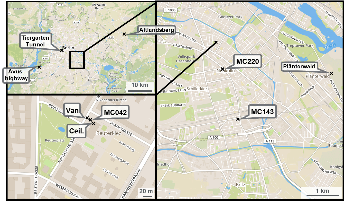
Figure 1Location of the measurement station (MC042) and measurement van in Neukölln, Berlin. Maps show increasingly larger scale. The “x”s indicate sampling locations, with MC220 and MC143 indicating stations that record traffic counts. Map images from OpenStreetMap.
The “Berlin Air quality and Ecosystem Research: Local and long-range Impact of anthropogenic and Natural hydrocarbons 2014” (BAERLIN2014) campaign aimed to address some of these issues in the context of the Berlin–Potsdam urban area. The campaign had three main aims: (1) characterization of gaseous and particulate pollution, including source attribution, in the Berlin–Potsdam area; (2) quantification of the role of natural sources, specifically vegetation, in determining levels of gaseous pollutants, specifically ozone; and (3) improved understanding of the heterogeneity of pollutants throughout the city. In this paper, only the first and second aims will be addressed. An overview paper describing the mobile measurements, which focused more on the third aim was published previously (see Bonn et al., 2016). Because of the focus on ozone and secondary pollutant formation, the campaign was conducted during the 3 summer months (June–August) of 2014, i.e., the time of maximum ozone pollution levels. Furthermore, while the mobile measurements covered the larger Berlin–Potsdam area, the stationary measurements were focused on an urban background location within the center of Berlin.
The unique characteristics of Berlin were particularly relevant to this study, in that it is a large urban area (population approximately 3.5 million) with significant vegetation. Of the approximately 890 km2 that Berlin covers, approximately 34 % of the land surface area is covered by vegetated areas and 6 % by water (Senatsverwaltung für Stadtentwicklung III F, 2010). An existing air quality monitoring network (in German: Berliner Luftgüte Messnetz, abbreviated BLUME) provided data on which the campaign could build and leverage. Data from the 16 stations that comprised the BLUME network showed that the EU 8 h ozone target value of 120 µg m−3 was exceeded 12–13 times at each of the two urban background stations that measure ozone (MC010 & MC042) and between 12 and 21 times per station at the stations on the periphery of the city (referred to here as Berlin rural stations) in 2014 (Stülpnagel et al., 2015). Six of these exceedances in the urban background occurred during the BAERLIN2014 campaign. Furthermore, the regulatory limit value for annual NO2 of 40 µg m−3 was exceeded at all six roadside stations in 2014 and, although the annual PM10 limit value was met, four out of five traffic stations where PM10 was measured also exceeded the daily limit value of 50 µg m−3 more than the allowed 35 times; the exceedances at the urban background and Berlin rural stations ranged from 14 to 34 times (Stülpnagel et al., 2015). In short, the issue of air pollution has been recognized in Berlin as being in need of action. In this paper, we focus on the stationary measurements conducted at the urban background site in the Berlin city center. A brief overview is given of the suite of measurements conducted and the results obtained. This is followed by more detailed analysis of (1) the NMVOC data and the role in ozone formation including a comparison to a previous study in London and Paris (von Schneidemesser et al., 2011), as well as other urban areas, and (2) source apportionment analysis of PM10 filter samples, including a rough comparison of the results to existing emission inventories.
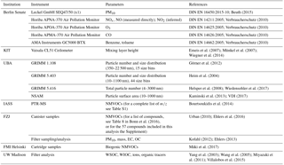
A complete list of the parameters measured and their associated instrument descriptions are summarized in Table 1.
Table 1List of participating institutions and instruments deployed at the urban background site in Berlin (Nansenstrasse).
2.1 Site description
The monitoring station that was the basis for the stationary measurements during the BAERLIN2014 campaign was AirBase station DEBE034, which is maintained as part of BLUME (network code MC042), and was located at the corner of Nansenstrasse and Framstrasse in the Neukölln district, in southeast central Berlin (52∘29′21,98 N, 13∘25′51,08 E) in a predominantly residential neighborhood, as shown in Fig. 1. The station was located on the street corner next to a kindergarten and was classified as an urban background station. According to the location placement dictated by the EU Directive definition (EC, 2008), locations that are situated away from any strong point sources including major roads, typically in a residential neighborhood, but still in the urban core influenced by all sources upwind of the station are classified as urban background. These sites should in theory be representative of the general levels of pollution observed in a city and are used to assess exposure of the general population to air pollutants. This station will likely experience a comparatively high fraction of traffic-related emissions, since some fairly large inner-city thoroughfares were located within a 1 km radius of the site, but as appropriate for an urban background station will not be dominated by traffic like a site located at a major intersection. In addition, a measurement van was used to augment the capacity of the measurement station and was located approximately 5 m from the station, parked at the curb of the street (see Fig. 1). Finally, owing to the presence of taller trees in that part of city, including in the vicinity of the monitoring station, one instrument (ceilometer) was located on the roof of the kindergarten to achieve an unobstructed view skywards, approximately 5 m on the opposite side of the measurement station to the van.
Table 2NMVOC canister sampling locations, site type, and average OH reactivity (s−1).
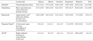
a Sampling duration of 20 min. All other samples had 10 min
sampling duration.
b Automated sampling while driving; all other samples are taken from a
stationary location.
A number of NMVOC canister samples were taken in locations throughout the city as part of the mobile measurements that augmented the stationary measurements in Neukölln. A subset of these were included in the companion paper to this one covering the mobile measurements (Bonn et al., 2016). These sites where multiple NMVOC canister samples were taken include Altlandsberg, Plänterwald, the Tiergarten Tunnel, and the so-called AVUS motorway during a traffic jam. Further details to the sampling environment can be found in Table 2. For more information on locations and/or sampling, see also Bonn et al. (2016).
2.2 Instrument descriptions
Complementing the BLUME measurements (see Stülpnagel et al., 2015, or Geiß et al., 2017, for details) were additional PM10 filter samples collected for elemental carbon (EC) and organic carbon (OC), ions, and organic tracer analysis; intermittent canister and cartridge samples for the quantification of NMVOCs from an inlet next to the PM10 inlet on the roof of the measurement station; a quadrupole proton transfer reaction mass spectrometer (high-sensitivity PTR-MS; Ionicon) up in the van for the measurement of NMVOCs; a set of particle instruments to measure number concentration, size distribution, and surface area also located in the van (Sect. 2.2.4); and a ceilometer CL51 (Vaisala GmbH, Hamburg) situated on the roof of the kindergarten. A complete list of instruments, parameters measured, and references for the methods used is provided in Table 1. Further details for the NMVOC measurements are provided in Table S1. Additional information is provided below.
2.2.1 NMVOC canister samples
The canisters were prepared to remove ozone using a heated Silcosteel capillary (120 ∘C) prior to sampling. The cylinders were then pressurized using synthetic air to reduce the relative humidity of the sample. All NMVOC canister samples taken at Neukölln had a 20 min sampling duration. After sampling, the canisters were promptly shipped to FZJ for analysis by gas chromatography (GC) flame ionization detector (FID) mass spectrometer (MS) and were analyzed with no more than 5 days between sampling and analysis. Analysis was done using a gas chromatographic system based on a conventional gas chromatograph (Agilent 6890) equipped with a FID and a MS (Agilent 5975C MSD) for the identification of the trace species. To analyze VOCs at trace gas levels, a cryogenic pre-concentration was used, consisting of a sample loop (Silcosteel, 20 cm length, inner diameter 2 mm) which was cooled down with cold gas above liquid nitrogen (see also Fig. 14 in Ehlers et al., 2016). A volume of 800 mL was pre-concentrated in the sample loop at a flow of 80 mL min−1.
Subsequently, the sample was thermally desorbed at 120 ∘C and injected on a capillary column (DB-1, 120 m, 0.32 mm ID, 3 µm film thickness). After injection, the column was kept isothermal at −60 ∘C for 5 min, then heated to 200 ∘C at a rate of 4∘ min−1 and finally maintained at 220 ∘C for 10 min. Signals were gathered from a flame ionization detector and a MSD, which each received 50 % of the column output through a split valve. Analysis of one sample lasted for about 90 min, and sets of 10 cylinders (stainless steel canister, volume: 6 L, Supelco Co., Bellefonte, PA, USA) could be analyzed by unattended operation.
The impact of canister transport and storage was assessed: C2–C11 alkanes, alkenes, and aromatic compounds were found to be stable within 5 % over 3 days compared with an instantaneously analyzed sample. Oxygenated compounds differed by up to 10 % and terpenes by up to 20 % over the same time period (Hengst, 2007). In addition, measurement accuracy depends on the uncertainty of the calibration standard (<5 % between true and declared gas concentrations; Apel-Riemer Environmental Inc.) and that of the mass-flow controller (<2 % deviation, MKS Instruments, Wilmington, MA, USA). Integration uncertainties (ΔμVOC) of the peak areas were dependent on their respective detection limits (DLi), which are estimated as in Eq. (1).
Apart from concentrations and their respective detection limits geometrical addition of all these factors yielded overall experimental uncertainties of less than 10 % (for a detailed discussion refer to Urban, 2010).
Canister samples and OH reactivity calculations
While a total of 103 compounds were quantified by GC-MS in the canister samples, not all of those compounds were regularly detected in the samples. Furthermore, to be able to make reasonable comparisons with previous work regarding the contribution of different compound classes to the measured mixing ratios of NMVOCs, as well as the OH reactivity attributed to these NMVOCs, a subset of the compounds was selected and used in the analysis. This subset was based on a number of papers in the literature that were also done in urban areas and those compounds that were regularly included in OH reactivity calculations (e.g Dolgorouky et al., 2012; Gilman et al., 2009; Goldan et al., 2004; Liu et al., 2008). This includes 57 NMVOCs (see Supplement). Furthermore, even if all compounds were included, there would still be missing reactivity that is not captured; because no OH measurements were made, the amount of missing reactivity cannot be reliably quantified, and therefore the measured OH reactivity here is a lower limit. Owing to an undetermined source of contamination at the urban background site, the measurement of n-butane was compromised and was therefore not included among the NMVOCs despite typically being reported in the literature. The data subsequently presented in this paper from the canister samples include only these 57 compounds unless otherwise noted. For a complete list of the 103 compounds measured in the samples, including the concentrations reported for a subset of the samples discussed here, please see Bonn et al. (2016).
A number of canister samples were taken at different locations throughout the city, some with multiple measurements and some single samples. Five locations had multiple samples, including the main measurement site at the urban background station (DEBE034) in Neukölln (n=18), Plänterwald (n=11), Altlandsberg (n=10), the Tiergarten Tunnel (n=9), and the AVUS motorway during a traffic jam (n=2). All samples were taken during the month of August, with all samples except those in Neukölln taken on 1 day for any given location (Bonn et al., 2016). The samples in the Tiergarten tunnel and on the motorway are most indicative of NMVOC emissions from traffic.
2.2.2 NMVOC cartridge samples
NMVOCs (aromatic hydrocarbons, terpenes, C6–C10 alkanes) were collected into stainless steel cartridges (6.3 mm ED × 90 mm, 5.5 mm ID) filled with Tenax-TA (60/80 mesh, Supelco, Bellafonte, USA) and Carboback-B (60/80 mesh, Supelco, Bellafonte, USA) by using a flow rate of 100 mL min−1 with a sampling time of 1–4.5 h (Mäki et al., 2017). To prevent the degradation of biogenic VOC by O3, a catalyst heated to 150 ∘C was used.
Individual VOCs were identified and quantified using a thermal desorption instrument (Perkin-Elmer TurboMatrixTM 650, Waltham, USA) connected to a gas chromatograph (Perkin-Elmer® Clarus® 600, Waltham, USA) with a DB-5MS (60, 0.25 mm, 1 µm) column and a mass selective detector (Perkin-Elmer® Clarus® 600T, Waltham, USA). Five-point calibration was utilized using liquid standards in methanol solutions. Standard solutions were injected onto adsorbent tubes that were flushed with nitrogen (HiQ N2 6.0 > 99.9999 %, Linde AG, Pullach, Germany) flow (100 mL min−1) for 10 min in order to remove methanol. For aromatic hydrocarbons (benzene, toluene, ethylbenzene, p∕m-xylene, styrene, o-xylene, propylbenzene, ethyltoluenes, trimethylbenzenes), detection limits (LODs) varied between 5 and 60 ng m−3; for C6–C10 alkanes (hexane, heptane, octane, nonane, decane) LODs were between 5 and 10 ng m−3 and for isoprene LOD was 21 ng m−3. The quantified monoterpenes were α-pinene, camphene, β-pinene, Δ3-carene, p-cymene, limonene, 1,8-cineol, nopinone, terpinolene, and bornyl acetate with limit of detection in the range of 3–17 ng m−3; sesquiterpenes were longicyclene, iso-longifolene, aromadendrene, β-caryophyllene, and α-humulene with LOD of 20 ng m−3.
2.2.3 NMVOC PTR-MS measurements
In addition to canister and cartridge samples, NMVOCs were continuously measured over time by a high-sensitivity PTR-MS (Ionicon, built in 2008) (Lindinger et al., 1993). In brief, NMVOCs with a higher proton affinity than water vapor were charged via H3O+ ions and subsequently mass selectively detected by applying a distinct electric field strength for the individual masses selected. More details on the techniques can be found elsewhere (Blake et al., 2009). In total, 72 selected NMVOCs were measured between 11 June and 29 August 2014 via a heated inlet (T=60 ∘C) at street level out of the street facing window of a measurement van (MW088) at approximately 2.5 m above surface. Note that this PTR-MS detected integer ion mass numbers only and no time-of-flight option was available for this version. Selection of masses were based on two aspects: typical mass to charge (m∕z) ratios for anthropogenic and biogenic sources like benzene, toluene, isoprene and terpenes and mass scan results conducted once a week throughout the campaign period. In this way some masses changed during the total observation time because of changed scan intensities and the limited number of masses to be selected. Time resolution was set to 270 s, i.e., 4.5 min. The dataset was averaged after the campaign for 30 min and 1 h for comparison with other less time resolved measurement data. The drift tube pressure (pdrift) was kept between 2.1 and 2.3 mbar with a mean of 2.2 mbar. The detection chamber pressure was kept at 2 × 10⁻⁵ mbar. The intensity of the reference ion signal for detection efficiency, i.e., , was recorded as (4.4 ± 1.0) × 107 counts per second. For more details on the setup, see Bourtsoukidis et al. (2014). A list of all recorded masses can be found in the supporting online information. Because the PTR-MS technique does not allow for a detailed chemical structure analysis, the cartridge and canister samples were used as complementary information as to the identity of masses with more than a single compound present.
2.2.4 Particle number concentration and surface area measurements
The aerosol inlet was located 3.5 m above ground, about 1 m above the measurement van roof, attached to an aerosol splitter (Leibniz Institute for Tropospheric Research (TROPOS), “Kuh”). A LVS pump (Leckel GmbH, Berlin) operated at 1 m3 h−1 corresponding to an aerosol flow of 138 cm3 s−1 and a PM10 head (Leckel GmbH, Berlin) suitable for cutoff at 10 µm with 2.3 m3 h−1 was used to reduce diffusion losses. This served all particle measurement instruments.
The instruments that measured particle number (PN) and particle size distribution included a GRIMM 1.108 (particle sizes in optical equivalent diameter, GRIMM Aerosol Technik GmbH & Co. KG, Ainring), GRIMM 5.403, and GRIMM 5.416 (particle sizes in mobility equivalent diameter). Sampling average was mostly 1 and 8 min for Grimm 5.403.
The GRIMM 5.416, a condensation particle counter with n-butanol, provided total PN count over a size range from 4 to 3000 nm at a flow rate of 1.5 L min−1, and the uncertainty for 1 min sampling was ± 0.1 % or ± 15 cm−3 (Helsper et al., 2008; Wiedensohler et al., 2017). The GRIMM 5.403, a scanning mobility particle sizer equipped with a long DMA combined with a CPC with n-butanol, measured PN concentrations with size distribution information for particles between 10 and 1100 nm at a sample flow rate of 0.3 L min−1 and a sheath flow rate of 3 L min−1. For technical details see Heim et al. (2004). The uncertainty associated with the measurement is size dependent, with an uncertainty range of 10–15 % in the lowermost size range and approximately 2–3 % in the upper size range, and a total of 44 size bins. The GRIMM 1.108, a portable laser aerosol spectrometer and dust monitor, measured PN concentration with size distribution information, covering 350–22500 nm, with a sampling flow rate of 1.5 L min−1. PN concentrations were determined for 15 size bins with an uncertainty of ±3 %. For technical details see Görner et al. (2012).
The TSI Nanoparticle Surface Area Monitor 3550 (NSAM) measured lung deposable surface area for particle sizes ranging from 10 to 1000 nm at a flow rate of 2.5 L min−1. These values are reported in units of µm2 cm−3 corresponding to empirically derived parameters that correspond to the regions where the particles are deposited in the lung. Alveolar deposition was measured. Measurement accuracy for the NSAM was ±20 % for both parameters. Further instrument and measurement details are described elsewhere (Kaminski et al., 2013; VDI, 2017).
The NSAM was calibrated at the German Environment Agency (UBA, Langen) with instruments from IUTA, Duisburg (Kaminski, 2011, personal communication), the GRIMM 1.108 was sent in for maintenance and re-calibrated at the manufacturer prior to use in the campaign, while all other instruments were calibrated a priori at the TROPOS aerosol calibration facility in Leipzig (Weinhold, 2014, personal communication).
A continuous aerosol size distribution (0.01 to 30 µm) was created using a combination of GRIMM 5.403 (0.01 to 1.1 µm) and GRIMM 1.108 (0.3 to 30 µm). Averaged 1 h size distribution from both particle instruments was merged to create a full size distribution from 0.01 to 30 µm. Size distributions from the two analyzers were merged by considering GRIMM 5.403 for particles sizes <1.1 µm and sizes equal or above 1.1 µm uses GRIMM 1.108. At 1.1 µm both individual logarithmic size bin boundaries of the 5.403 and 1.108 were most similar allowing “a smooth merge” without losing any size bins. We also assumed that the particles were spherical and thus no adjustments were made in the size bins nor were any adjustments made for possible differences in aerodynamic vs. optical derivation of diameter.
2.2.5 Ceilometer
State-of-the-art ceilometers provide the vertical profile of aerosol backscatter (Wiegner et al., 2014). There are numerous approaches to estimate the mixing layer height (MLH) from the measured profile; the underlying assumption is that at the top of the mixing layer aerosol concentration drastically drops resulting in a pronounced decrease of backscattered signal intensity. Measurements in the framework of BAERLIN2014 were performed with a Vaisala ceilometer CL51 (Münkel, 2007; Geiß et al., 2017). This instrument is eye-safe (class 1M) with fully automated and unattended operation. The diode laser emits at a wavelength of 910 nm; the absorption by water vapor can be ignored as long as only the MLH is to be determined (Wiegner and Gasteiger, 2015). Laser power and window contamination are permanently monitored to ensure long-term stability. Due to the one-lens design the lowest detectable layers are around 50 m, and the system is capable of covering an altitude range greater than 4000 m, topping out around 8 km. Signals are pre-processed, e.g., for the suppression of noise-generated artifacts. The range resolution is 10 m, and the temporal averaging is 10 min.
The heights of the near surface aerosol layers were analyzed by a gradient method from the backscatter profiles in real time (Emeis et al., 2008) with a MATLAB-based software which is provided by the manufacturer and has been improved continuously (Münkel et al., 2011). The minima of the vertical gradient is used to provide an estimate of the MLH (Emeis et al., 2007). All MLH data presented follow this method (for more detail see Schäfer et al., 2015) unless otherwise noted. The influence of different options of the proprietary software and an comparison with the more sophisticated approach COBOLT (COntinuous BOundary Layer Tracing) on the retrieved MLH is discussed in detail by Geiß et al. (2017). It was found that the proprietary software slightly tends to overestimate the MLH compared to COBOLT.
The various instruments outlined above had differing sampling times and so for those instruments that provided real-time or higher time resolution data, a 30 min average will be used in the data presented here for comparability.
2.2.6 PM10 filter analysis
Prior to sampling, the quartz fiber filters were baked at 800 ∘C under synthetic air to remove impurities. Post-sampling, the PM10 filters were analyzed for total mass, elemental carbon (EC), water-soluble and total organic carbon, chloride, sulfate, nitrate, sodium, ammonium, potassium, calcium, and organic tracers. HYSPLIT back trajectories (based on GDAS meteorological data) were calculated for 72 h over the time period of each filter with a new trajectory each 6 h for air masses ending at ground level (at the monitoring station) (Stein et al., 2015). Back trajectory plots are included in the Supplement following the final filter groups. Based on similarities in the bulk composition analysis and HYSPLIT back trajectory information, the filters were grouped before being extracted and analyzed for organic tracers. Not all filters were included in these groups, so as to create groups that showed significant similarities. Some individual filters were therefore also excluded from the organic tracer analysis because of a lack of remaining OC mass.
PM10 mass was first quantified gravimetrically and then analyzed for elemental and organic carbon. For this the filter samples were heated to 750 ∘C in an oxygen stream. The gas stream was then passed through an oxidation catalyst to ensure complete oxidation of the organic carbon to carbon dioxide (CO2). In contrast to the organic carbon, elemental carbon is directly oxidized at higher temperatures without the requirement of a catalyst. The organic carbon, as CO2, was then detected using a cavity ring-down spectrometer (Picarro Inc.). The distinction between the elemental and organic carbon fractions in the samples was based on the temperature profile during the analysis. For more details see Ehlers (2013) and Kofahl (2012).
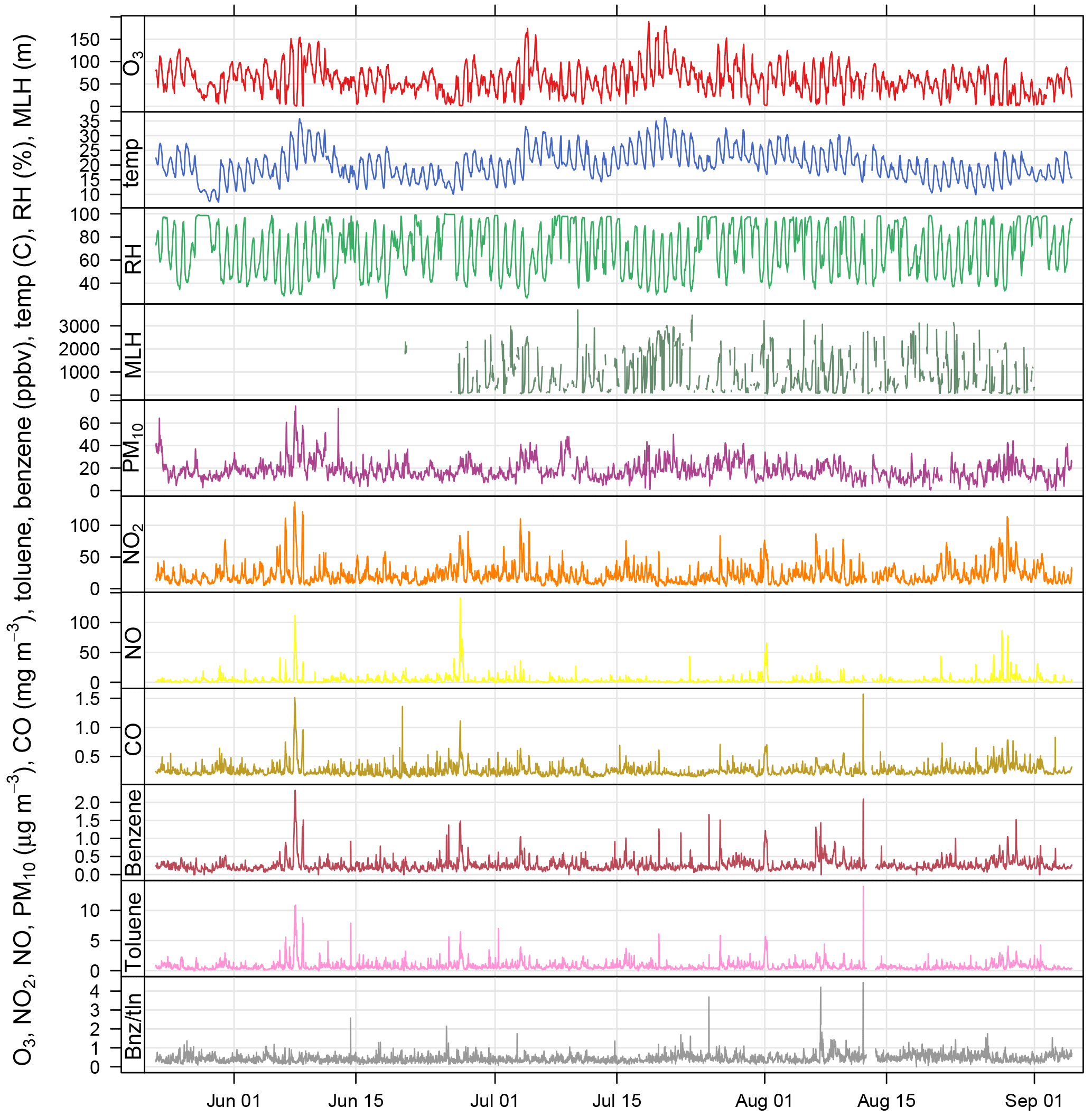
Figure 2Time series of air pollutant concentrations, meteorological data, and benzene / toluene ratio measured as part of BLUME at the Neukölln station during the BAERLIN2014 campaign.
A portion of the filter (1.5 cm2) was water extracted to determine water-soluble organic carbon (WSOC) using a TOC-V SCH Shimadzu total organic carbon analyzer (Miyazaki et al., 2011; Yang et al., 2003). The remaining amount of OC was calculated as water-insoluble organic carbon (WIOC). A fraction of the remaining solution was used to analyze for water-soluble anions and cations by ion chromatography (Dionex ICS 2100 and Dionex ICS 100) (Wang et al., 2005). For the organic tracer analysis, filters were composited as per the bulk composition and HYSPLIT determined groups and extracted with 50/50 dichloromethane and acetone by sonication, an aliquot was derivatized and analyzed by GC-MS (GC-6980, quadropole MS-5973, Agilent Technology) for organic molecular marker compounds, as described in more detail by Villalobos et al. (2015) and references therein. Approximately 150 organic tracer species were analyzed for, of which less than 100 had concentrations regularly above the detection limit. A limited subset of these was then used in the source apportionment analysis.
2.3 Chemical mass balance for source apportionment
A chemical mass balance analysis of the organic carbon fraction of the PM10 filter samples was carried out using the organic tracer information. Source apportionment analysis using the CMB technique provides an effective variance least squares solution for a set of linear equations that include the uncertainties of the input measurements and have been applied to the mass balance receptor model (Watson et al., 1984). As such, it allows for the estimation of the contribution of different source categories to the ambient concentrations measured at any one location, in this case an urban background site in Berlin. The species included in the CMB analysis were levoglucosan, 17α(H)-21β(H)-30-norhopane, 17α(H)-21β(H)-hopane, benzo(b)fluoranthene, benzo(k)fluoranthene, benzo(e)pyrene, benzo(a)pyrene, and C27–C33 alkanes. The US EPA CMB Software version 8.2 was used. Source profiles for vegetative detritus (Rogge et al., 1993), wood burning (Fine et al., 2004), and diesel and gasoline motor vehicles (Lough et al., 2007) were included in the final result. In addition, a profile for poorly maintained vehicles (“smoking vehicles”) (Lough et al., 2007) was evaluated but found inappropriate. The link between tracers and sources is discussed in further detail in Sect. 3.5.2. The SOA fraction was calculated based on WSOC not related to biomass burning (Sannigrahi et al., 2006). The fitting statistics for the final result are shown in Table 3.
Table 3Basic bulk composition results, ratios, and air mass origin from HYSPLIT. Units are µg m−3 unless otherwise noted. For OC and EC measurement uncertainty is included.
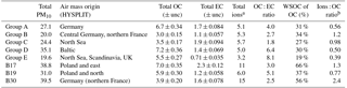
a Ions include seven species and are not limited to sulfate, nitrate, and
ammonium.
b Ratio of ions (sulfate, nitrate, ammonium) to OC.
3.1 Time series and diurnal cycle
The 30 min data time series of O3, NO2, NO, CO, benzene, toluene, and PM10, along with basic meteorological data from the BLUME station in Neukölln and MLH as derived from the proprietary software are shown in Fig. 2, spanning the duration of the campaign. All times are given in CET. The 8 h mean ozone concentrations show that the EU target value for ozone (120 µg m−3 based on 8 h means) was exceeded 6 times during the measurement period, and the WHO guideline (100 µg m−3) was exceeded 18 times. The hourly limit value for NO2 (200 µg m−3) was not exceeded, though concentrations often exceeded 100 µg m−3. The daily limit value for PM10 (50 µg m−3) was not exceeded.
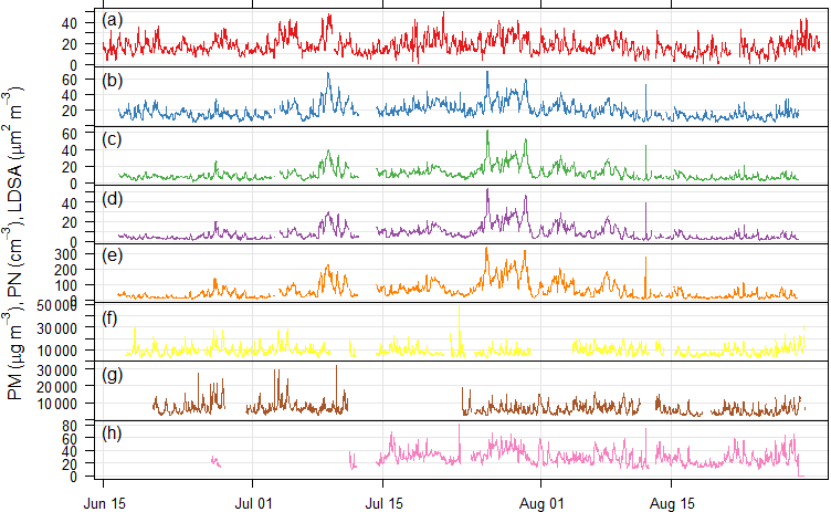
Figure 3Time series of particulate matter mass, particle number, and lung depositable surface area concentrations measured at the Neukölln station during the BAERLIN2014 campaign. (a) BLUME PM10, (b) Grimm 1.108 PM10, (c) Grimm 1.108 PM2.5, (d) Grimm 1.108 PM1, (e) Grimm 1.108 PN, (f) Grimm 5.416 PN, (g) Grimm 5.403 PN, and (h) NSAM LDSA. Units given in the y-axis label.
Elevated concentrations were often observed at the same time for many of the pollutants included in Fig. 2, with the exception of ozone. Ozone, as a secondary pollutant formed photochemically from NOx and NMVOC precursors, follows a similar pattern to temperature (Pearson correlation coefficient (SE) of 0.82 (0.014)) and peaks at different times than the primary pollutants. The formation of ozone can be limited by either NOx or NMVOCs, depending on the ambient concentrations which are controlled by sources (e.g., vehicles, biogenics) and transport. NO2, NO, CO, toluene, and benzene all have diurnal cycles that peak in the morning and evening, reflecting their anthropogenic traffic-related emission sources (see Fig. S1 in the Supplement). The morning peak in the pollutants occurred at 07:00 or 08:00, while the evening peak occurred quite late between 21:00 and 23:00, likely owing to a combination of daytime emissions and the decrease in the MLH. Traffic counts, from MC143 and MC220 in Neukölln (see location in Fig. 1), showed that traffic increased dramatically between 06:00 and 08:00–09:00, after which a slow but steady increase led to a peak at 17:00–18:00, after which the traffic count dropped dramatically. In contrast, ozone, temperature, and MLH followed parallel diurnal cycles with a minimum at 06:00 and a broad afternoon peak between noon and 18:00. During BAERLIN2014 the maximum height of the mixing layer was found to be 1.5–2 km between noon and 18:00 and below 500 m during the night/early morning. These numbers indicate the vertical extent of the urban pollution layer over the measurement site where pollutants are most likely residing. Relative humidity showed the opposite with a peak at 06:00 and a broad low between noon and 18:00.

Figure 4Mean diurnal cycles of the (a) particle number and (b) particle volume distributions at Neukölln. Legends show particle size bin range in nanometers.
These results are supported by the Pearson correlation coefficients among NO2, NO, CO, toluene, and benzene, which for hourly values range from 0.51 to 0.82 (all statistically significant at an alpha = 0.05; see Table S2), with the strongest relationship between CO and NO2. The correlation to relative humidity was found to be negative for MLH (−0.66 (0.022)), temperature (−0.71 (0.014)), and ozone (−0.76 (0.014)). The pollutant with the strongest relationship to temperature was ozone.
The time series of particulate matter mass (PM10), derived PM1, PM2.5, and PM10 mass from the GRIMM 1.108 particle number size distribution measurements, total particle number, and particle surface area are shown in Fig. 3. While the two PM10 time series along with the PM and particle number time series associated to the same instrument (GRIMM 1.108) are most similar, the other total particle number time series do not show significant similarities. This is largely due to the difference in size fractions measured by the different instruments. Correlation analysis of the pollutant concentrations from Neukölln with MLH values on the basis of averaged diurnal cycles of hourly-mean values (in our case monthly averages during July and August) provided highest correlations with PN for accumulation mode particles (size range 100–500 nm) and significant correlations for PM2.5 and PM1 (Schäfer et al., 2015) showing similarities to investigations in Augsburg, Germany (Schäfer et al., 2016), and Beijing, China (Tang et al., 2016). In addition to this investigation for the reference site, a more detailed correlation analysis of the MLH with PM10, O3, and NOx taking into account all 16 BLUME stations in Berlin was carried out using the MATLAB approach outlined here as well as an alternative approach, COBOLT (Geiß et al., 2017). In this context it was assumed that the MLH derived for the reference site in Neukölln is representative for the entire metropolitan area of Berlin. The correlation analysis of the diurnal cycles (averaged over the duration of ceilometer measurements from BAERLIN2014) of the MLH and PM10 found that correlations were completely different at the different sites regardless of site type, indicating that surface concentrations of PM10 were not predominantly determined by the MLH, but rather by local sources and sinks and meteorological factors, among others. In the case of O3, strong positive correlations were identified for both the BLUME sites on the periphery of Berlin, as well as the urban background locations. In contrast, for NO2, a negative correlation to MLH was observed for all sites at the periphery of the city and to a lesser extent at some of the urban background sites (Geiß et al., 2017).

Particle size distribution during the study period is shown in Fig. 4. Size distribution was dominated by ultrafine number size distribution (UFP, <100 nm) throughout the day (i.e., particle formation close by). The number and volume distribution was further binned into at least 5 size bins, as presented in Fig. 4 for comparison with other urban background measurements. The average daytime total number and volume concentration remained in the range of 5.5–6.0 × 103 cm−3 and 11–12 µm3 cm−3, respectively, in contrast to the stronger signal during the nighttime. The mean (median) total number and volume concentration over the entire measurement period was 6.1 × 10³ (5.4 × 103 cm−3) and 11.8 µm3 cm−3 (9.5 µm3 cm−3), respectively. Over 80 % of the total number concentration is ultrafine particles, and the contribution is higher during the nighttime. Volume distribution is largely dominated by the accumulation mode particles, which is typical of many urban sites. The number concentrations were similar to other urban stations in Germany (Birmili et al., 2016).
The diurnal cycles for total PN for the three instruments covering the smaller particles (excluding the observations from the GRIMM 1.108) have morning and evening peaks, similar to the diurnal cycle for NO2, indicating a traffic origin. The diurnal cycle for the larger particles, as sampled by the GRIMM 1.108 has a much more dominant early morning peak and mid-afternoon minimum, without the second evening peak.
In Fig. 5, at least two major contributors to UFP over the course of the day could be identified, in the morning and during the night. The presence of the morning peak is likely due to traffic-related emissions. Such a peak has also been identified in other species, as well as other studies in urban areas (Borsós et al., 2012; Mølgaard et al., 2013). There was a gradual increase in the UFP concentration from late afternoon which continued overnight until early morning hours. This nighttime feature of UFP was observed during weekends as well as on the weekdays. The reasons for this could be that the source contributing to this is something other than or in addition to traffic and may be active or enhanced overnight, the decrease in mixing layer height at night traps the particles in a smaller volume compared to daytime, and/or that nighttime deposition of particles is lower than daytime due to higher atmospheric stability. The co-located trace gas measurement showed that the elevated UFP nighttime concentration correlates with toluene, among other gases such as CO. Daily observations also showed occasional and episodic “particle burst” (new particle formation) events for particles in the size range of 10–50 nm, which could be related to fresh plumes or to regional particle formation events.
3.2 NMVOC measurements – method comparison
The results of the four NMVOC measurement methods were compared and contrasted for benzene and toluene. While differences in, for example, instrumentation and measurement technique (mass-to-charge (m∕z) ratios vs. compounds), inlet location, and time resolution do not allow for direct comparisons, a comparison can be useful to understand how different or similar the information provided by the various methods can be. A summary of these methods and the compounds measured, including information on the detection limits and sampling times, is provided in Table S1.
The 30 min data reported from the BLUME city air quality monitoring network were compared to the PTR-MS data for m∕z 79 (benzene) and m∕z 93 (toluene), as both instruments provide data of high time resolution. The correlations between the two methods were good given the imperfect nature of the comparison, both with Pearson's r values for benzene and toluene of 0.39, significant at the p<0.05 level. The lower correlation values were likely due to a number of factors including the differences in measurement method and location of the inlets for each instrument and thereby source influences – one of which (PTR-MS) was located on the street side of the van at approximately 2.5 m above ground, while the other (BLUME) was located above the measurement container approximately 5 m from the street. The inlet at the street would be influenced more directly by vehicle emissions in comparison to the inlet above the measurement container, which is especially relevant in that the PTR-MS was likely influence by individual vehicles, while this would not be the case for the container measurements. This influence of vehicles on the PTR-MS data at higher time resolution is supported by an increase in Pearson's r values with longer averaging times, which reduces the influence of individual vehicles. For 1 h (3 h) average concentrations the r values increase to 0.48 (0.58) and 0.53 (0.71) for benzene and toluene, respectively, all significant at the p<0.05 level. Furthermore, the Pearson's r values for the correlations between the BLUME network and the individual canisters were 0.39 (benzene) and 0.83 (toluene), both statistically significant with p values < 0.05, and between BLUME and the cartridge samples 0.51 (toluene) and not significant for benzene. All benzene and toluene measurements are shown in Fig. S2.
In order to investigate the possibility of identifying molecular structures of m∕z measurements derived by PTR-MS, a comparison of the continuous measurements of the PTR-MS and intermittent canister samples was also carried out. For a number of cases only one compound quantified from the canister samples matched a specific m∕z, while in other cases multiple compounds were quantified in the canister samples that had the same mass. For example, propanal, acetone, n-butane, and 2-methylpropane all have a molecular weight corresponding to m∕z 59 (molar weight MW=58 g mole−1 + MW(H g mole−1), among which the PTR-MS cannot distinguish. In some cases, the fractional contribution of compounds with the same m∕z ratio was relatively similar across all canister samples, as for o-xylene, m+p-xylene, and ethylbenzene (m∕z 107). However, this was rather the exception, with relative contributions more typically showing significant variation among the canister samples (see Fig. S3 in the Supplement). Correlations between the canister samples and PTR-MS results were carried out for 35 individual m∕z values for which at least one compound was quantified in the canister samples. While the absolute r values of the correlations ranged from 0.00016 to 0.63, the correlations were generally quite poor, showing little to no correlation for many of the m∕z (only 9 of the 35 total number of m∕z values evaluated had r values greater than 0.3), with no systematic bias identified. There are a number of reasons for this, beyond the difference in how the instruments measure (m∕z vs. compounds), such as inlet location and sampling time. Previously, in a targeted intercomparison experiment where whole air samples (canisters) were compared with online PTR-MS measurements, differences of as little as 20 s in the sampling intervals contributed to scatter in the comparison of the two measurements that was especially relevant for the more reactive NMVOCs (de Gouw and Warneke, 2006). Additionally, scatter in intercomparisons between ground-based fast time response and GC-MS systems was found to be typical (Lerner et al., 2017, and references therein). In the context of this study, the measurements should not be considered as an intercomparison since, as described above, the inlets were approximately 5 m apart, at different heights above ground level, with one street-side and the other above a measurement container. For these reasons, while both measurements are valid, as this comparison shows, the differences in quantification method, but also importantly instrument location and setup, result in substantial differences in what is being quantified so that the comparison is limited in value.

Figure 6Mean fractional contribution to mixing ratio (a) and OH reactivity (b) by compound class, based on a total mixing ratio or OH reactivity calculated from 57 compounds for 5 sampling locations throughout the city. Total number of canister samples for each location are Neukölln (18), Altlandsberg (10), Plänterwald (11), Tiergarten Tunnel (9), and the AVUS motorway (2). The individual compounds included in each class are available in the Supplement.
3.3 NMVOC measurements – characterization of different locations by canister sampling
The average fractional contribution to mixing ratio by compound class for each of the Neukölln, Altlandsberg, Plänterwald sites, the Tiergarten tunnel, and the AVUS motorway samples is presented in Fig. 6. The number of compounds included in each class was alkanes (19), alkenes and alkynes (13), aromatics (14), oxygenated (6), and biogenics and their oxidation products (5; referred to as “biogenics” for simplicity). For a complete list of the compounds and their grouping, see the Supplement. In the following text and figures two extremely high values for acetone were removed (one sample from the Neukölln station and one from the Altlandsberg samples). Since these two values were extreme outliers, their origin remains unclear. Therefore we have removed them from the averages and treated them separately. (Text is included in the Supplement to demonstrate how these two values change the results presented here.) The largest contributions of the quantified VOCs to mixing ratio were from the alkanes (27–41 %) and oxygenated (23–55 %) compounds. Biogenics were always a minor contribution to mixing ratio, but their contribution was largest in the Plänterwald samples (11 %) and negligible at the two traffic locations. Alkenes/alkynes and aromatics showed the largest contribution to mixing ratio at the traffic sites, at 17–23 and 14 %, respectively. The highest total NMVOC mixing ratio of those compounds measured here was found at the traffic sites (Tiergarten tunnel, 64 ± 17 ppbv; AVUS motorway, 170 ± 82 ppbv; average mixing ratio ± standard deviation among the samples). The total mixing ratio of the 57 measured compounds at Altlandsberg and at the urban background station in Neukölln showed similar results, with an average mixing ratio and standard deviation of 14 ± 6.4 ppbv and 19 ± 5.6 ppbv, respectively. The mixing ratios found in Plänterwald were similar to the urban background location, with an average of 17 ± 3.4 ppbv, although with a larger contribution from biogenics. In comparison, total non-methane hydrocarbon (NMHC) mixing ratios for urban background in Paris during the MEGAPOLI winter campaign was 12 ppbv (midnight median levels) or 17 ppbv (maximum of median daily values), with somewhat lower mixing ratios measured during the summer campaign (Dolgorouky et al., 2012; Ait-Helal et al., 2014).
Previously, a measurement campaign was carried out during June–August 1996 in Berlin, during which samples were taken at the Neukölln urban background station, as well as at a traffic station on Frankfurter Allee. During this campaign, VOC measurements were taken 4 times a day for 2 h over the course of 1 week (7 days) of each month using bag samples, adsorption tubes and DNPH cartridges and analyzed by gas chromatography (Thijsse et al., 1999). This provides a good basis for comparison to the NMVOCs measured by canister sampling (most similar in method) during this campaign almost 20 years later. Overall, the mixing ratios for most compounds that were measured in both projects at the urban background location in Neukölln were lower now than in 1996 (Fig. 7). For the traffic locations the results are less clear. Given that the Frankfurter Allee monitoring station is a traffic station, these measurements would likely be more comparable to the Tiergarten Tunnel measurements of this study than those samples taken during a traffic jam on the AVUS motorway where concentrations were extremely elevated. Indeed, the mixing ratios measured during the traffic jam were found to be higher in most cases than those measured in 1996 at Frankfurter Allee. However, the comparison between the Tiergarten Tunnel measurements and Frankfurter Allee showed much more similar results to those of the urban background station comparison, with concentrations generally being lower today than approximately 20 years ago (Thijsse et al., 1999).
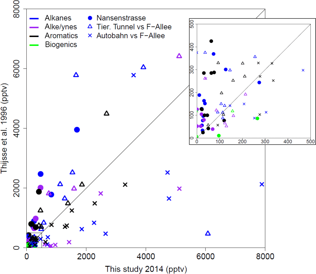
Figure 7Comparison between VOC measurements in this study and comparable previous work from June to August 1996 (Thijsse et al., 1999). Compound classes are distinguished by color. Sampling locations by plotting character.
There are a couple of exceptions in this comparison, where the mixing ratios measured in this campaign stand out as substantially higher than those measured 20 years ago. Considering only those few compounds that have a ratio of 0.6 or less for the average mixing ratio in 1996 relative to that in 2014, the biogenic contributions in Neukölln (isoprene (0.3), methyl vinyl ketone (0.1)) show increases. These increases may be attributable to changes in vegetation around the measurement site. Other NMVOCs, such as cis-2-butene and cyclopentane, showed increases for both the urban background site and traffic site (Tiergarten Tunnel vs. Frankfurter Allee). Other compounds, such as cis-2-pentene and trans-2-butene (traffic site) and 1,2,3-trimethylbenzene (urban background), showed increases at only the one site type. While the literature on trends of NMVOCs is limited, data from a traffic site in London, a rural background site in the UK, and a remote site in Germany showed that over the period from 1998 to 2009 all individual NMVOCs evaluated (with the exception of n-heptane at the rural background site) were decreasing, with stronger decreases observed at the traffic site relative to the other site types (von Schneidemesser et al., 2010). Similarly, an evaluation of C2–C8 hydrocarbon data, as total hydrocarbons and by compound class, for a number of sites across the UK from 1994 to 2012, also documented decreases across all compound classes (Derwent et al., 2014). Finally, a broader evaluation of the trends in anthropogenic NMVOC emissions across Europe also documented a decrease between 2003 and 2012 (EEA, 2014, 2016). As such, the existing literature does not provide any detailed documentation that might be able to address the potential increases in those few compounds here where an increase was observed. Furthermore, longer-term sampling may show that the increases documented here do not reflect the long-term trend.
3.4 OH reactivity
To better understand the role of these compounds with respect to their role in ozone formation and the reactivity of the measured compounds, the reactivity with respect to OH (ROH) was calculated. These results are shown in Fig. 6 and parallel the results presented for the mixing ratios. In all cases, including other studies discussed, the values presented are calculated OH reactivity based on measurements of NMVOCs and not OH reactivity that was measured directly. Because the OH reactivity estimates are based on a limited number of NMVOCs, the values presented here are a lower limit. The relative importance of the biogenics, alkenes, and alkynes, and to a lesser extent the aromatics, increased when considering OH reactivity, as is visible in Fig. 6 (for a complete list of compounds included in these classes, see the Supplement). The largest contribution to OH reactivity was from either the biogenics and their oxidation products (0–75 %) or the alkenes and alkynes (10–55 %), depending on the location, with the alkenes and alkynes dominating at the traffic locations, where the biogenic contribution was negligible. The NMVOCs included in each of these categories are provided in Sect. S1. The contribution to OH reactivity from alkanes ranged from 4 % (Plänterwald) to 18 % (AVUS motorway). The contribution from oxygenated compounds, despite their substantial contribution to mixing ratio, ranged from only 5 to 13 % of OH reactivity. That said, only 6 oxygenated NMVOCs (of 57 total NMVOCs) were included here, and a recent study by Karl et al. (2018) found an appreciably greater fraction of oxygenated NMVOCs in urban areas than previous studies identified. The molar flux of oxygenated NMVOCs being actively emitted into the urban atmosphere from measurements in Europe was found to be 56 ± 10 % relative to the total NMVOC flux (Karl et al., 2018), which indicates that a much larger contribution from oxygenated NMVOCs is possible if different measurement techniques are used. The contribution to the biogenic OH reactivity at Plänterwald originated largely from isoprene (88 %), with 7 % from α- and β-pinene. Similar contributions were found at Neukölln and Altlandsberg. The mean (median; 25th and 75th percentiles) total OH reactivity from the 57 species was 2.6 s−1 (2.6; 2.1, 3.0 s−1) at Neukölln and ranged from 2.2 s−1 (2.2; 1.5, 2.8 s−1) at Altlandsberg to 34 s−1 (34; 29, 39 s−1) at the AVUS motorway. While studies have shown that a number of NMVOCs, such as isoprene, or other terpenes can also have anthropogenic sources (Derwent et al., 2007; Reimann et al., 2000), we treat them as biogenic and do not try to tease apart the biogenic vs. potential anthropogenic contributions in this context.
An earlier study (BERLIOZ) also made measurements of C2–C12 NMHCs in Berlin and at sites in the surrounding area, mostly focused on the production of ozone in downwind locations of the city (Winkler et al., 2002; Volz-Thomas et al., 2003; Becker et al., 2002). They report OH reactivity for two sites outside of Berlin: Blossin (approximately 15–20 km southeast of the Berlin city boundary) and Pabstthum (approximately 30–35 km northwest of the Berlin city boundary). The total OH reactivity reported at these sites range between 1 and 7 s−1 and between approximately 0.25 and 2 s−1, respectively. These are similar to those values found at the urban background locations in Berlin, with the most comparable location being Altlandsberg (2.2 s−1). The contribution from isoprene to the OH reactivity was found to be 70 % at Blossin and 51 % at Pabstthum, on average, although during the passing of a city plume at Pabstthum 46 % of reactivity was contributed by isoprene, with the remaining contribution attributed to anthropogenic NMHCs (Winkler et al., 2002).
The total OH reactivity values of measured VOCs in Berlin (2.6 s−1) are similar to the average total OH reactivity from VOCs observed in other European cities, such as Paris (approximately 4.0 s−1) and London (1.8 s−1) (Dolgorouky et al., 2012; Whalley et al., 2016), and, not surprisingly, lower than those observed at cities in the Pearl River Delta region of China (8–14 s−1). Specifically, Liu et al. (2008) reported OH reactivity from a measurement campaign in Ghangzhou and Xinken during 1 month in the autumn of 2004. The OH reactivity from alkanes, alkenes, and aromatics from Ghangzhou was reported to be 1.9 ± 1.5, 8.8 ± 6.8, and 2.9 ± 2.7 s−1, respectively. In all cases, these values are about 1 order of magnitude greater than those calculated for the urban background locations during this campaign (see Table 2). The level for isoprene (0.5 ± 0.4 s−1), however, was much more similar to the OH reactivity reported for the biogenics at the urban background locations in this study. In London, OH reactivity of alkanes, alkenes + alkynes, aromatics, and biogenics was reported to be 0.81, 0.47, 0.235, and 0.25 s−1, respectively, which are values much more similar to those in this study (Whalley et al., 2016). The relative importance of alkanes and alkenes + alkynes was the reverse for London compared to Berlin.
In the MEGAPOLI winter campaign in Paris, total calculated mean OH reactivity was reported to be 17.5 s−1, although this included not only NMVOCs but also methane, CO, NO, and NO2 (Dolgorouky et al., 2012). The OH reactivity attributed to the 29 NMHCs and oxygenated VOCs was 23 % (4.0 s−1) of the total, somewhat higher than those values reported here (57 NMVOCs) for the urban background locations. Comparing to the OH reactivity values in Berlin is difficult, since for the winter campaign in Paris, Ait-Helal et al. (2014) report that the concentrations of the VOCs are generally shown to be lower during summer, specifically for many of the anthropogenic compounds, although this does vary by compound. Therefore, the OH reactivity values for Paris considered here should be considered an upper limit for the comparison with this study. The calculated mean OH reactivity attributed to NO and CO was 1.75 s−1 each and 9.63 s−1 for NO2 in Paris (Dolgorouky et al., 2012). By comparison, the mean OH reactivity calculated for August (to match the time during which the canister samples were taken at Neukölln) was 0.58 ± 1.2 and 0.87 ± 0.30 s−1 for NO and CO, respectively, and 4.5 ± 3.0 s−1 for NO2, which is again lower as with the VOCs, but not unreasonable given the context of the comparison.
Finally, while the 57 NMVOCs included here to calculate OH reactivity were chosen to facilitate comparison to previous studies, a more exhaustive list could change the picture. For example, as mentioned above, the limited number of oxygenated NMVOCs measured would likely lessen the contributions of the other compound classes. As an example, adding six additional oxygenated NMVOCs (propanal, 2-butanol, 1-propanol, butanal, 1-butanol, pentanal) increased the total average OH reactivity between 0.12 s−1 (Plänterwald) and 1.7 s−1 (AVUS Motorway). The percent contribution of these six oxygenated NMVOCs ranges between 2.5 and 9.3 % of the new total OH reactivity. In contrast, a similar analysis that included three additional biogenic NMVOCs (limonene, sabinene, eucalyptol) showed much smaller additional reactivity – never more than 0.02 s−1. These compounds also were not consistently present across all samples.
3.4.1 OH reactivity – direct comparison to a previous study in London and Paris
As a comparison to the ROH estimates calculated for London and Paris based on approximately 10 years of monitoring data through 2009 (von Schneidemesser et al., 2011), a subset of the NMVOCs was taken to enable a more equal comparison to the values reported for summer (JJA) in that study. The only difference in the compounds included is the contribution of n-butane, which was not included in the Berlin calculations because of a local source of contamination (in London the contribution of n-butane to OH reactivity from this subset of NMVOCs was approximately 5 % or less). The referenced study was focused on the contribution of biogenics, specifically isoprene, to OH reactivity. At the London Eltham site (urban background) isoprene contributed 25 % to the OH reactivity for summer and 16 % at Paris Les Halles, also an urban background location (24 total NMVOCs, including 9 alkanes, 9 alkenes/alkynes, 5 aromatics, 0 oxygenated, 1 biogenic) (von Schneidemesser et al., 2011). Using the reduced, matched set of compounds, isoprene accounts for 37 % of OH reactivity at the Neukölln location on average and as much as 82 % at the Plänterwald (urban park) location in Berlin. The Neukölln urban background location values are a bit higher than those in London and Paris, although not dramatically different. The Plänterwald urban park location, however, demonstrates the importance of such areas for the biogenic influence on OH reactivity, especially considering that even at Harwell, a rural background location west of London in the UK, isoprene contributes on average only 10 % of OH reactivity. Although, as pointed out in the study, this is likely an underestimation of the biogenic importance given that only isoprene is included and for northerly regions other biogenics, such as monoterpenes, may play a more important role (von Schneidemesser et al., 2011).
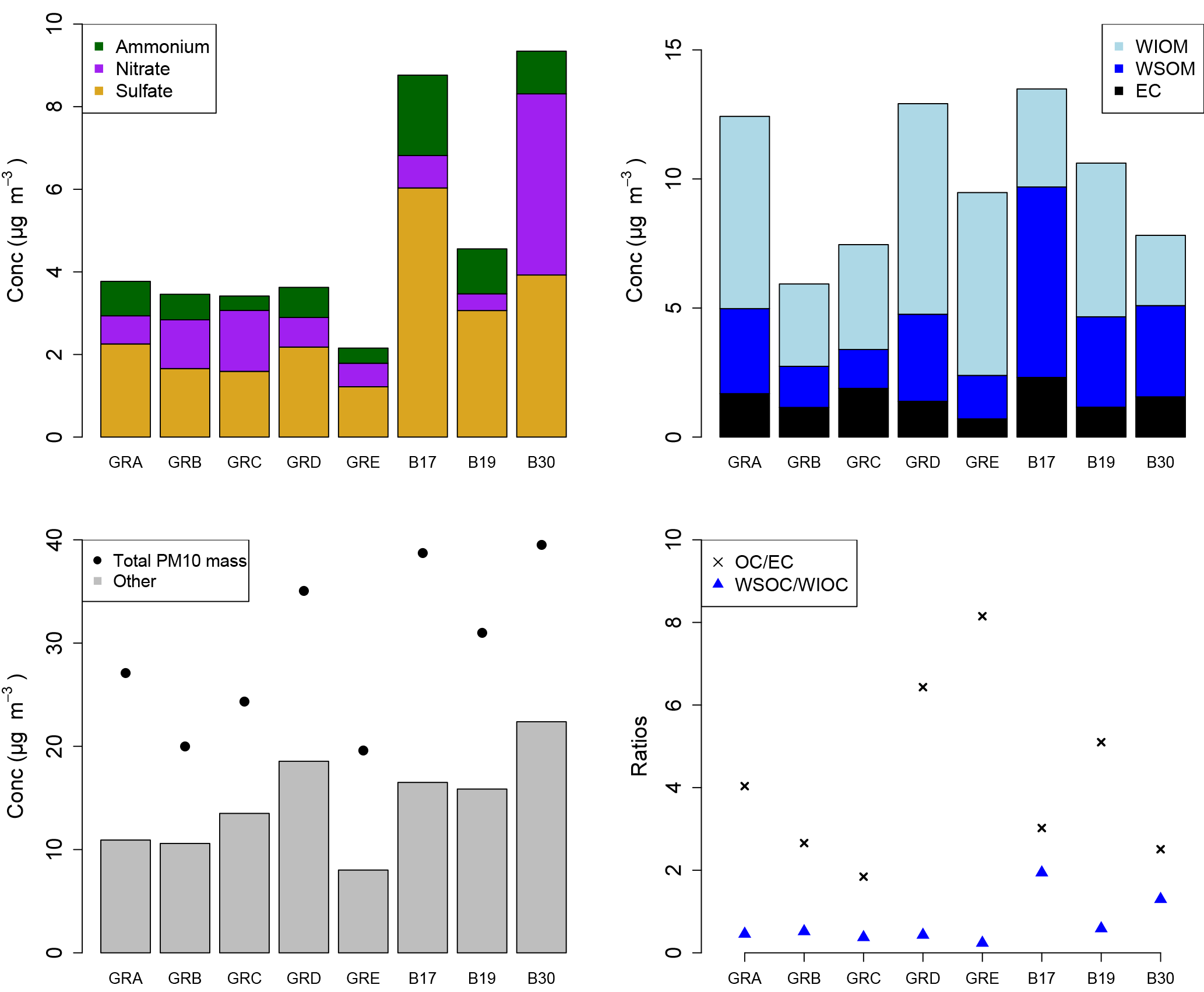
Figure 8Bulk composition analysis results from the PM10 filter samples, presented by filter groups, where GRA is group A, GRB is group B, etc. and B17, B19, and B30 are individual filters. More information on the filter groups, including some basic composition information and back trajectory origin, can be found in Table 3.
3.5 PM10 filters
3.5.1 Bulk composition and HYSPLIT back trajectories
The PM10 filters were analyzed for water-soluble and water-insoluble OC, EC, and ions. In addition, filter samples were grouped to ensure enough mass for analysis of organic molecular markers. The groups were informed by the bulk composition analysis results, including the ratio of water-soluble to total OC and the ratio of ions to OC, and HYSPLIT back trajectories. Back trajectories were evaluated to provide information on the origin of the air masses and source-receptor relationships (Stein et al., 2015). The results of this bulk composition analysis are shown in Fig. 8. Select individual filters that had sufficient mass and did not fit with any of the other groups were analyzed individually (B17, B19, B30). All values listed for groups are an average of the results from the filters included in the group. The air mass origins as per HYSPLIT are summarized in Table 3 (see also Fig. S4).
Groups A, B, C, and D show significant similarity in their percent of OC that is WSOC, which ranges from 27 to 34 %. The ratio of ions (sulfate, nitrate, ammonium) to OC is, however, very different. Groups B and C have an ions : OC ratio of 1.2 and 0.98, while groups A and D have ratios of 0.56 and 0.50, respectively. The PM10 mass loadings for B (20 µg m−3) and C (24 µg m−3) were lower than for A (27 µg m−3) and D (35 µg m−3); see Table 3. The concentrations of EC ranged between 1.1 and 1.9 µg m−3 but did not group as with the other species, with the lowest concentration in group B and the highest in group C.
Group E had a very low percent of WSOC (19 %) and an ions : OC ratio of 0.59. It also had the lowest PM10 mass (20 µg m−3) and either the lowest or among the lowest concentrations for all ions. The OC concentration, however, was 5.5 µg m−3, which was roughly in the middle of the OC concentrations measured, while the EC concentration was also the lowest at 0.71 µg m−3.
B17, B19, and B30 were analyzed individually because their bulk composition analysis and back trajectory patterns did not group well with the others, and sufficient mass was available for tracer analysis without needing to composite filters (Table 3, Fig. 8). B17 and B30 had a higher percent WSOC (66 and 56 %, respectively) and ions : OC ratios of 1.3 and 2.4, respectively. For B19, 37 % of OC was WSOC and the ions : OC ratio was 0.77. Total PM10 mass was 38.8, 31.0, and 39.5 µg m−3, and OC concentrations were 7.0, 5.9, and 3.9 µg m−3, for B17, B19, and B30, respectively. All three samples had significantly larger contributions from sulfate, and to a lesser extent also higher ammonium, compared to the other groups. B30 also has a large amount of nitrate in contrast to all other samples and somewhat higher concentrations of potassium and sodium as well. B17 had the highest concentration of EC (2.3 µg m−3) of all samples.
There were significant concentrations of sulfate across all samples, ranging from 1.2 to 6.0 µg m−3, but particularly so in B17, B19, and B30. Sulfate is typically attributed to industrial sources, as the content of sulfate in fuels has been reduced significantly and is now quite low (Villalobos et al., 2015). Sea salt is in this case not likely as a source, as Berlin is not within close proximity of a coastal region where such components are typically identified (Putaud et al., 2004). In general the significant contributions of sulfate, nitrate, and ammonium are indicative of a secondary inorganic aerosol (ammonium sulfate and ammonium nitrate) (Putaud et al., 2004; Schauer et al., 1996). Previous work has shown that secondary inorganic aerosol over northwestern Europe, including Germany, contribute significantly – about 50 % – to the PM10 concentrations (Banzhaf et al., 2013). Two studies by Putaud et al. (2004, 2010) summarize the relative contribution of major constituent chemical species to PM mass, including for near-city and urban background locations. In comparison to the numbers cited in that study (2004 all European sites; 2010 northwestern European sites), the percent contribution of nitrate (15; 14 %), ammonium (7 %; not listed), and sulfate (13; 14 %) to PM10 mass at the urban background site in Berlin were quite similar, ranging from 1 to 11 % (nitrate), 1 to 5 % (ammonium), and 6 to 16 % (sulfate) in Berlin.
The back trajectories (Fig. S4) show that prior to arriving in Berlin, the air masses primarily passed over Germany for group A. While some additional filters fit the general patterns outlined here, the number of filters included in the group was reduced to focus more on back trajectories in the group that originated from over Germany itself. The air masses that characterize group D originated from the northeast, passing over the Baltic coast and Poland before arriving in Berlin. For group B the air masses originated from the west over the Atlantic (not further than 20∘ W) and passed over northern France, the Benelux region, and central Germany before arriving in Berlin. For group C, the air masses originated from the northwest, over the North Sea as far as Iceland, passing between the UK and the Scandinavian Peninsula before arriving in Berlin. Both B and C had higher concentrations of sodium and nitrate than A and D, while A and D had higher concentrations of OC and marginally higher concentrations of sulfate than B and C (Fig. 8). The air masses of group E originated from the north, passing over Scandinavia, the North Sea, or the UK before arriving in Berlin. The back trajectories associated with B17 and B19 both passed over Poland before arriving in Berlin, with the air masses associated with B19 extending more northward as well. For B30 the air originates from the west with some passing over northern France, but mostly comes from over Germany itself. The significant presence of ammonium and sulfate likely indicates influence of agriculture, as ammonium sulfate is commonly used in fertilizer and more than 95 % of NH3 emissions in Europe originate from agriculture (Harrison and Webb, 2001; Backes et al., 2016; EEA, 2016).

Figure 9Molecular marker analysis results from the PM10 filter samples, presented by filter groups, where GRA is group A, GRB is group B, etc. and B17, B19, and B30 are individual filters. More information on the filter groups, including some basic composition information and back trajectory origin, can be found in Table 3.
3.5.2 Organic molecular markers
The concentrations by composited sample are shown in Fig. 9 for the organic molecular markers. Levoglucosan has been established as a molecular marker for biomass burning (Simoneit et al., 1999). The concentrations measured here ranged from 15 to 60 ng m−3. While high concentrations of levoglucosan in urban areas are often associated with residential wood combustion during colder months, it can also be due to crop burning, wild fires, coal combustion, and/or long-range transport of smoke from biomass burning (Simoneit, 2002; Zhang et al., 2008; Shen et al., 2016). The concentrations measured during this summer campaign in Berlin were similar to those measured in PM10 from other European cities during summertime and approximately an order of magnitude lower than concentrations observed in winter (Caseiro and Oliveira, 2012, and references therein). The study by Caseiro and Oliveira (2012) confirms the likelihood of agricultural residue burning and/or wildfires as a summertime source for levoglucosan.
Alkanes are useful tracers to distinguish between fossil fuel sources and vegetative detritus. This distinction is informed by the odd–even carbon number predominance, specifically of the C29, C31, and C33 n-alkanes to indicate plant material as a source (Rogge et al., 1993). As is visible in Fig. 9, the concentrations of those odd n-alkanes are much greater than the corresponding even n-alkanes. Furthermore, the carbon preference index (CPI) was calculated for the samples using the C29–C33 n-alkanes and ranged from 1.9 to 5.5, with an average of 3.6. CPI values of approximately 1 are indicative of fossil fuel emission sources, whereas values of approximately 2 or greater are indicative of biogenic detritus (Simoneit, 1986), as is clearly the case for these samples.
Hopanes have been established as markers for diesel and gasoline vehicle emissions, stemming from petroleum product utilization and lubricating oil used in vehicles (Schauer et al., 1996; Rushdi et al., 2006; Simoneit, 1984). The concentrations of the two hopanes measured here and included in the CMB analysis ranged from 0.04 to 0.13 ng m−3 as shown in Fig. 9.

Figure 10Source contributions attributed to the OC fraction of the PM10 filter samples by filter groups, where GRA is group A, GRB is group B, etc. and B17, B19, and B30 are individual filters. More information on the filter groups, including some basic composition information and back trajectory origin, can be found in Table 3.
Polycyclic aromatic hydrocarbons (PAHs) are formed and emitted most typically during the incomplete combustion of fossil fuels or wood (Ravindra et al., 2008). The concentrations measured during this study ranged from 0 to 0.23 ng m−3 for the individual PAHs shown in Fig. 9. These concentrations are similar to, although on the lower end of, those measured in a study in Flanders, Belgium, including measurements at urban locations (Ravindra et al., 2006). Generally, PAH concentrations are lower in summertime owing to lower emissions and shorter lifetimes. The measurements here were conducted during summer, while the measurements in the study in Flanders covered more seasons. To distinguish between sources, PAH concentration profiles or ratios are used. For example, a ratio of benzo(b)fluoranthene to benzo(k)fluoranthene of greater than 0.5 has been identified as an indicator for diesel emissions sources (Park et al., 2002; Ravindra et al., 2008). In this study the ratio ranged from 1.9 to 7.2, indicating a strong influence of diesel emissions for these compounds.
3.5.3 Chemical mass balance
The molecular markers analyzed in the organic carbon fraction of the PM10 samples were used to conduct source apportionment analysis using chemical mass balance. The total OC for these samples ranged from 2.99 to 7.21 µg m−3. The amount of OC mass apportioned in the CMB analysis ranged from 21 to 49 %. The source profiles included in the model to which OC was attributed includes vegetative detritus, diesel emissions, gasoline vehicle emissions, and wood burning. In addition, a fraction of the unapportioned OC was attributed to SOA based on the unapportioned fraction of water-soluble OC and the amount attributed to wood burning, following Sannigrahi et al. (2006). The source contributions to OC, as well as the fitting statistics, are listed in Table 4, and shown in Fig. 10.
Table 4Chemical mass balance source apportionment results. Units are µg m−3 unless otherwise noted. Uncertainty is measurement uncertainty, in the case of SOA propagated uncertainty, and SE is standard error for the source categories.
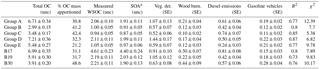
a The SOA contribution was not part of the CMB results, but rather calculated as unapportioned WSOC (SOA) = measured WSOC – 0.71a apportioned wood burning.
For B17, B19, and B30 the SOA fraction is higher than for any of the others, at 63, 34, and 49 % of OC, respectively. They also had the highest concentrations of levoglucosan, ranging from 37.8 to 60.1 ng m−3. As the primary tracer for biomass burning, these three samples also had the largest concentrations attributed to this source, ranging from 0.22 to 0.44 µg m−3 of OC, but the relative contribution was only larger for B30 at 11%. All other samples had contributions that ranged between 2 and 4 % of OC. These three samples had air masses that originated over Poland (B17, B19) and Germany (B30), indicating a more local–regional source for the biomass burning. The higher concentrations of potassium in these samples, also an indicator for biomass burning (Andreae, 1983), provide additional confirmation. The relatively high concentrations of ammonium and sulfate in these samples may indicate an agricultural influence. Those samples originating from regions to the west and north had somewhat lower concentrations overall relative to those originating from regions to the east and north, as shown in Fig. 10.
The contribution of diesel emissions ranged from 0.24 to 0.81 µg m−3, corresponding to 4–21 % of OC fraction. The highest fractional contribution was found in group C (concentration 0.74 µg m−3) (air masses originating over the North Sea), while the highest concentration was found in sample B17 (fractional contribution 12 %) (from Poland to the east). The diesel from group C could also have its origin in shipping emissions, as well as diesel vehicles. High contributions of diesel did not necessarily correspond to high contributions of gasoline vehicle emissions, which were lower than the contributions from diesel and ranged from 0.11 to 0.28 µg m−3 and 2 to 7 % of OC. The highest contribution in terms of fractional contribution and concentration was found in B30. Furthermore, it should be noted that the source profiles reflect primary organic aerosol emissions, and therefore the secondary aerosol produced from these vehicular sources (which has been shown to be substantial in many cases, depending on the control technologies in use; Gordon et al., 2014a, b), is not reflected in these attributions.
The contribution of vegetative detritus was among the largest source contributions and ranged from 0.51 to 1.4 µg m−3 (11–20 %). The relative importance of this source is reflected in the concentrations of the alkanes, as shown in Fig. 9, and their average CPI of 3.6. The largest contribution was found for group D with air masses originating over the North Sea.
For all samples, a significant amount of SOA was calculated: 0.87–4.4 µg m−3 (18–63 %). While this was the contribution to OC, high concentrations of secondary inorganics (sulfate, ammonium, nitrate) support the aging of the air masses and the potential for a significant contribution from secondary aerosol overall.
It should be noted that ambient air samples include contributions from both local sources and locations further away. While the back trajectory analysis is more relevant for interpreting the influence of emissions from the surrounding region, a comparison to the Berlin emission inventory reflects on the influence of local source contributions. Both play a role, but neither capture the complete picture, with limitations in both cases, as discussed further below.
3.5.4 Source apportionment – emission inventory comparison
The source apportionment results were compared to the emissions inventory (EI) from TNO-MACC III (Kuenen et al., 2014). The grid cells for Berlin were extracted and the percent of total emissions for OC by source category for the Berlin area for June, July, and August as a rough comparison to the source apportionment results was calculated. Both diesel and gasoline vehicle exhaust sources have significant contributions, although diesel contributes approximately 19 % to total OC emissions in the inventory, whereas gasoline vehicles contribute only about 1 %. Biogenic sources are not included in the inventory. If we focus on the primary sources from the source apportionment results, the diesel and gasoline vehicles contribute a significant fraction, with diesel comprising a larger fraction than gasoline vehicles, as in the inventory. The inventory also includes significant contributions from road transport originating from road, brake, and tire wear, which are not reflected in the CMB results due to the profiles used. About 8 % of OC emissions are attributed to agriculture in the EI. This could contribute to both the biomass burning and vegetative detritus sources; the presence of significant secondary ammonium and nitrate also indicates an agricultural influence, even though this does not show up in the OC CMB. In all cases, these primary sources will contribute to secondary inorganic and organic aerosol formation. The contributions from non-industrial combustion and energy and other industries are not captured as primary source contributions in the CMB model. Overall, the comparison between the source apportionment results and the EI is a non-ideal comparison given the differences in methodology and the difference in terms of primary vs. secondary sources that are or are not included. More specifically, the EI provides primary emissions estimates for a year for all Berlin grid cells (Kuenen et al., 2014), while the CMB results provide source attribution to ambient concentrations including primary and secondary sources for 3 months of summer at one location in Berlin. However, one would expect that general patterns are captured for significant sources, as it was for vehicle emissions, and the indication of agriculture.
The data presented here provide an overview of the stationary measurements conducted during the BAERLIN2014 campaign. Of the three main aims of the campaign, two were addressed here, including (1) characterization of gaseous and particulate pollution, including source attribution, in the Berlin–Potsdam area, and (2) quantification of the role of natural sources, especially vegetation, in determining levels of gaseous pollutants such as ozone. PM10 concentrations and the contributions from inorganic species, such as nitrate, sulfate, and ammonium that contribute substantially (10–24 %) to secondary aerosol, were found to be similar in terms of their relative contribution to PM10 in other European cities. Both the PM and gas-phase pollutants exhibited diurnal cycles indicative of anthropogenic sources, and the ratio of benzene to toluene indicated the influence of fresh, local emissions. Comparison of canister samples taken over the course of a day showed similarities which would seem to imply an urban background level for many NMVOC species. In addition to the secondary inorganic aerosol, a significant fraction of OC was attributed to secondary organic aerosol (18–63 %) in the CMB analysis.
The influence of vegetation and biogenic emissions was demonstrated in the canister sample analysis, as well as the CMB results where vegetative detritus comprised one of the larger sources contributing to the OC fraction, ranging from 11 to 20 %. While the detected mixing ratios of the biogenic NMVOCs did not contribute significantly to the total NMVOC mixing ratio, the role in, for example, ozone formation, assessed by calculating OH reactivity, was much more significant. Biogenics and their oxidation products accounted for 31 % of the OH reactivity at the urban background station in Neukölln and 75 % at the urban park location (Plänterwald), demonstrating the importance of urban parks for biogenic emissions. These contributions from biogenics were higher than those found at comparable urban background locations in London and Paris. This is likely linked to the relatively high amount of land surface area in Berlin covered by vegetated areas (34%). It should, however, be acknowledged that only a subset of the total NMVOCs were measured. If all “missing” NMVOCs were measured it could influence our results, including the contribution of biogenics and other compound classes to the calculated OH reactivity.
As an outlook, future research could build on this work to include additional analysis of PTR-MS data using positive matrix factorization to investigate the sources influencing NMVOC concentrations at the Neukölln location as well as modeling studies to gain greater insight as to the impact of urban vegetation on ozone formation, both yielding further insight into the importance of biogenic VOCs in urban environments.
The datasets generated during and/or analyzed during the current study are available from the corresponding author on request.
The supplement related to this article is available online at: https://doi.org/10.5194/acp-18-8621-2018-supplement.
The authors declare that they have no conflict of interest.
This work was hosted by IASS Potsdam, with financial support provided by the
Federal Ministry of Education and Research of Germany (BMBF) and the
Ministry for Science, Research and Culture of the State of Brandenburg
(MWFK). The authors would like to thank Hugo Denier van der Gon and Jeroen
Kuenen (TNO) for providing information pertaining to the TNO-MACCIII
inventory and Friderike Kuik for the Berlin emissions processing; Christoph
Münkel from Vaisala GmbH, Hamburg, for support with ceilometer CL51 data
analyses to determine mixing layer heights; Wolfram Birmili (UBA), Alfred
Wiedensohler, and Kay Weinhold (TROPOS) for discussions informing the
particle measurements; and colleagues at the IASS for their support of the
campaign and discussions that helped shape the manuscript. The authors
gratefully acknowledge the NOAA Air Resources Laboratory (ARL) for the
provision of the HYSPLIT transport and dispersion model and/or READY website
(http://www.ready.noaa.gov, last access: 19 March 2015) used in this publication. Boris Bonn
thankfully
acknowledges a grant from the IASS to support the studies.
Edited by: Thomas Karl
Reviewed by: two anonymous referees
Ait-Helal, W., Borbon, A., Sauvage, S., de Gouw, J. A., Colomb, A., Gros, V., Freutel, F., Crippa, M., Afif, C., Baltensperger, U., Beekmann, M., Doussin, J.-F., Durand-Jolibois, R., Fronval, I., Grand, N., Leonardis, T., Lopez, M., Michoud, V., Miet, K., Perrier, S., Prévôt, A. S. H., Schneider, J., Siour, G., Zapf, P., and Locoge, N.: Volatile and intermediate volatility organic compounds in suburban Paris: variability, origin and importance for SOA formation, Atmos. Chem. Phys., 14, 10439–10464, https://doi.org/10.5194/acp-14-10439-2014, 2014.
Andreae, M. O.: Soot carbon and excess fine potassium: long-range transport of combustion-derived aerosols, Science (New York, N.Y.), 220, 1148–1151, https://doi.org/10.1126/science.220.4602.1148, 1983.
Backes, A. M., Aulinger, A., Bieser, J., Matthias, V., and Quante, M.: Ammonia emissions in Europe, part II: How ammonia emission abatement strategies affect secondary aerosols, Atmos. Environ., 126, 153–161, https://doi.org/10.1016/j.atmosenv.2015.11.039, 2016.
Banzhaf, S., Schaap, M., Wichink Kruit, R. J., Denier van der Gon, H. A. C., Stern, R., and Builtjes, P. J. H.: Impact of emission changes on secondary inorganic aerosol episodes across Germany, Atmos. Chem. Phys., 13, 11675–11693, https://doi.org/10.5194/acp-13-11675-2013, 2013.
Becker, A., Scherer, B., Memmesheimer, M., and Geiß, H.: Studying the city plume of Berlin on 20 July 1998 with three different modelling approaches, J. Atmos. Chem., 42, 41–70, https://doi.org/10.1023/A:1015776331339, 2002.
Birmili, W., Weinhold, K., Rasch, F., Sonntag, A., Sun, J., Merkel, M., Wiedensohler, A., Bastian, S., Schladitz, A., Löschau, G., Cyrys, J., Pitz, M., Gu, J., Kusch, T., Flentje, H., Quass, U., Kaminski, H., Kuhlbusch, T. A. J., Meinhardt, F., Schwerin, A., Bath, O., Ries, L., Gerwig, H., Wirtz, K., and Fiebig, M.: Long-term observations of tropospheric particle number size distributions and equivalent black carbon mass concentrations in the German Ultrafine Aerosol Network (GUAN), Earth Syst. Sci. Data, 8, 355–382, https://doi.org/10.5194/essd-8-355-2016, 2016.
Blake, R. S., Monks, P. S., and Ellis, A. M.: Proton-Transfer Reaction Mass Spectrometry, Chem. Rev., 109, 861–896, 10.1021/cr800364q, 2009.
Bonn, B., von Schneidemesser, E., Andrich, D., Quedenau, J., Gerwig, H., Lüdecke, A., Kura, J., Pietsch, A., Ehlers, C., Klemp, D., Kofahl, C., Nothard, R., Kerschbaumer, A., Junkermann, W., Grote, R., Pohl, T., Weber, K., Lode, B., Schönberger, P., Churkina, G., Butler, T. M., and Lawrence, M. G.: BAERLIN2014 –the influence of land surface types on and the horizontal heterogeneity of air pollutant levels in Berlin, Atmos. Chem. Phys., 16, 7785–7811, https://doi.org/10.5194/acp-16-7785-2016, 2016.
Borsós, T., Řimnáčová, D., Ždímal, V., Smolík, J., Wagner, Z., Weidinger, T., Burkart, J., Steiner, G., Reischl, G., Hitzenberger, R., Schwarz, J., and Salma, I.: Comparison of particulate number concentrations in three Central European capital cities, Sci. Tot. Environ., 433, 418–426, https://doi.org/10.1016/j.scitotenv.2012.06.052, 2012.
Bourtsoukidis, E., Williams, J., Kesselmeier, J., Jacobi, S., and Bonn, B.: From emissions to ambient mixing ratios: online seasonal field measurements of volatile organic compounds over a Norway spruce-dominated forest in central Germany, Atmos. Chem. Phys., 14, 6495–6510, https://doi.org/10.5194/acp-14-6495-2014, 2014.
Brauer, M., Freedman, G., Frostad, J., van Donkelaar, A., Martin, R. V., Dentener, F., Dingenen, R. v., Estep, K., Amini, H., Apte, J. S., Balakrishnan, K., Barregard, L., Broday, D., Feigin, V., Ghosh, S., Hopke, P. K., Knibbs, L. D., Kokubo, Y., Liu, Y., Ma, S., Morawska, L., Sangrador, J. L. T., Shaddick, G., Anderson, H. R., Vos, T., Forouzanfar, M. H., Burnett, R. T., and Cohen, A.: Ambient Air Pollution Exposure Estimation for the Global Burden of Disease 2013, Environ. Sci. Technol., 50, 79–88, https://doi.org/10.1021/acs.est.5b03709, 2016.
Caseiro, A. and Oliveira, C.: Variations in wood burning organic marker concentrations in the atmospheres of four European cities, J. Environ. Monitor., 14, 2261–2269, https://doi.org/10.1039/c2em10849f, 2012.
Colette, A., Bessagnet, B., Vautard, R., Szopa, S., Rao, S., Schucht, S., Klimont, Z., Menut, L., Clain, G., Meleux, F., Curci, G., and Rouïl, L.: European atmosphere in 2050, a regional air quality and climate perspective under CMIP5 scenarios, Atmos. Chem. Phys., 13, 7451–7471, https://doi.org/10.5194/acp-13-7451-2013, 2013.
de Gouw, J. and Warneke, C.: Measurements of volatile organic compounds in the earth's atmosphere using proton-transfer-reaction mass spectrometry, Mass Spectrom. Rev., 26, 223–257, https://doi.org/10.1002/mas.20119, 2006.
Derwent, R. G., Jenkin, M. E., Passant, N. R., and Pilling, M. J.: Photochemical ozone creation potentials (POCPs) for different emission sources of organic compounds under European conditions estimated with a Master Chemical Mechanism, Atmos. Environ., 41, 2570–2579, https://doi.org/10.1016/j.atmosenv.2006.11.019, 2007.
Derwent, R. G.: New Directions: Prospects for regional ozone in north-west Europe, Atmos. Environ., 42, 1958–1960, 2008.
Derwent, R. G., Dernie, J. I. R., Dollard, G. J., Dumitrean, P., Mitchell, R. F., Murrells, T. P., Telling, S. P., and Field, R. A.: Twenty years of continuous high time resolution volatile organic compound monitoring in the United Kingdom from 1993 to 2012, Atmos. Environ., 99, 239–247, https://doi.org/10.1016/j.atmosenv.2014.10.001, 2014.
Dolgorouky, C., Gros, V., Sarda-Esteve, R., Sinha, V., Williams, J., Marchand, N., Sauvage, S., Poulain, L., Sciare, J., and Bonsang, B.: Total OH reactivity measurements in Paris during the 2010 MEGAPOLI winter campaign, Atmos. Chem. Phys., 12, 9593–9612, https://doi.org/10.5194/acp-12-9593-2012, 2012.
EC: Directive 2008/50/EC of the European Parliament and of the Council of 21 May 2008 on ambient air quality and cleaner air for Europe, in: 2008/50/EC, edited by: Union, E. P. a. t. C. o. t. E., Official Journal of the European Union, 2008.
EEA: Air quality in Europe – 2014 report, European Environment Agency, Luxembourg, 2014.
EEA: Air quality in Europe – 2016 report, European Environment Agency, Luxembourg, 2016.
Ehlers, C.: Mobile Messungen: Messung und Bewertung von Verkehrsemissionen, PhD, Mathematisch-Naturwissenschaftliche Fakultät, Universität Köln, 2013.
Ehlers, C., Klemp, D., Rohrer, F., Mihelcic, D., Wegener, R., Kiendler-Scharr, A., and Wahner, A.: Twenty years of ambient observations of nitrogen oxides and specified hydrocarbons in air masses dominated by traffic emissions in Germany, Faraday Discussions, 189, 407–437, https://doi.org/10.1039/C5FD00180C, 2016.
Emeis, S., Jahn, C., Münkel, C., Münsterer, C., and Schäfer, K.: Multiple atmospheric layering and mixing-layer height in the Inn valley observed by remote sensing, Meteorologische Zeitschrift, 16, 415–424, https://doi.org/10.1127/0941-2948/2007/0203, 2007.
Emeis, S., Schäfer, K., and Münkel, C.: Surface-based remote sensing of the mixing-layer height a review, Meteorologische Zeitschrift, 17, 621–630, https://doi.org/10.1127/0941-2948/2008/0312, 2008.
Fine, P. M., Cass, G. R., and Simoneit, B. R. T.: Chemical Characterization of Fine Particle Emissions from the Fireplace Combustion of Wood Types Grown in the Midwestern and Western United States, Environ. Eng. Sci., 21, 387–409, https://doi.org/10.1089/109287504323067021, 2004.
Geels, C., Andersson, C., Hänninen, O., Lansø, A., Schwarze, P., Skjøth, C., and Brandt, J.: Future Premature Mortality Due to O3, Secondary Inorganic Aerosols and Primary PM in Europe – Sensitivity to Changes in Climate, Anthropogenic Emissions, Population and Building Stock, Int. J. Environ. Res. Publ. Health, 12, 2837–2869, https://doi.org/10.3390/ijerph120302837, 2015.
Geiß, A., Wiegner, M., Bonn, B., Schäfer, K., Forkel, R., von Schneidemesser, E., Münkel, C., Chan, K. L., and Nothard, R.: Mixing layer height as an indicator for urban air quality?, Atmospheric Measurement Techniques, 10, 2969–2988, https://doi.org/10.5194/amt-10-2969-2017, 2017.
Gilman, J. B., Kuster, W. C., Goldan, P. D., Herndon, S. C., Zahniser, M. S., Tucker, S. C., Brewer, W. A., Lerner, B. M., Williams, E. J., Harley, R. A., Fehsenfeld, F. C., Warneke, C., and de Gouw, J. A.: Measurements of volatile organic compounds during the 2006 TexAQS/GoMACCS campaign: Industrial influences, regional characteristics, and diurnal dependencies of the OH reactivity, J. Geophys. Res.-Atmos., 114, https://doi.org/10.1029/2008JD011525, 2009.
Goldan, P. D., Kuster, W. C., Williams, E., Murphy, P. C., Fehsenfeld, F. C., and Meagher, J.: Nonmethane hydrocarbon and oxy hydrocarbon measurements during the 2002 New England Air Quality Study, J. Geophys. Res., 109, D21309, https://doi.org/10.1029/2003JD004455, 2004.
Gordon, T. D., Presto, A. A., May, A. A., Nguyen, N. T., Lipsky, E. M., Donahue, N. M., Gutierrez, A., Zhang, M., Maddox, C., Rieger, P., Chattopadhyay, S., Maldonado, H., Maricq, M. M., and Robinson, A. L.: Secondary organic aerosol formation exceeds primary particulate matter emissions for light-duty gasoline vehicles, Atmos. Chem. Phys., 14, 4661–4678, https://doi.org/10.5194/acp-14-4661-2014, 2014a.
Gordon, T. D., Presto, A. A., Nguyen, N. T., Robertson, W. H., Na, K., Sahay, K. N., Zhang, M., Maddox, C., Rieger, P., Chattopadhyay, S., Maldonado, H., Maricq, M. M., and Robinson, A. L.: Secondary organic aerosol production from diesel vehicle exhaust: impact of aftertreatment, fuel chemistry and driving cycle, Atmos. Chem. Phys., 14, 4643–4659, https://doi.org/10.5194/acp-14-4643-2014, 2014b.
Görner, P., Simon, X., Bémer, D., and Lidén, G.: Workplace aerosol mass concentration measurement using optical particle counters, J. Environ. Monitor., 14, 420–428, 2012.
Harrison, R. and Webb, J.: A review of the effect of N fertilizer type on gaseous emissions, in: Advances in Agronomy, Academic Press, 65–108, 2001.
Heim, M., Kasper, G., Reischl, G. P., and Gerhart, C.: Performance of a New Commercial Electrical Mobility Spectrometer, Aerosol Sci. Technol., 38, 3–14, https://doi.org/10.1080/02786820490519252, 2004.
Helsper, C., Horn, H.-G., Schneider, F., Wehner, B., and Wiedensohler, A.: Intercomparison of five mobility size spectrometers for measuring atmospheric submicrometer aerosol particles, Partikelmesstechnik, 68, 475–481, 2008.
Hengst, M.: Flüchtige Organische Verbindungen in der Ausatemluft von Kindern und Jugendlichen mit Asthma Bronchiale, PhD, Medizinischen Fakultät, Rheinisch-Westfälischen Technischen Hochschule Aachen, Aachen, Deutschland, 2007.
Jacob, D. J. and Winner, D. A.: Effect of climate change on air quality, Atmos. Environ., 43, 51–63, https://doi.org/10.1016/j.atmosenv.2008.09.051, 2009.
Kaminski, H., Kuhlbusch, T. A. J., Rath, S., Götz, U., Sprenger, M., Wels, D., Polloczek, J., Bachmann, V., Dziurowitz, N., Kiesling, H.-J., Schwiegelshohn, A., Monz, C., Dahmann, D., and Asbach, C.: Comparability of mobility particle sizers and diffusion chargers, J. Aerosol Sci., 57, 156–178, https://doi.org/10.1016/j.jaerosci.2012.10.008, 2013.
Karl, T., Striednig, M., Graus, M., Hammerle, A., and Wohlfahrt, G.: Urban flux measurements reveal a large pool of oxygenated volatile organic compound emissions, P. Natl. Acad. Sci., https://doi.org/10.1073/pnas.1714715115, 2018.
Kofahl, C.: Hochempfindliche Bestimmung der organischen und anorganischen Kohlenstoff-Fraktion in Feinstaubproben mittels CRD-Spektroskopie, BS, Chemie und Biotechnologie, Fachhochschule Aachen, 2012.
Kuenen, J. J. P., Visschedijk, A. J. H., Jozwicka, M., and Denier van der Gon, H. A. C.: TNO-MACC_II emission inventory; a multi-year (2003–2009) consistent high-resolution European emission inventory for air quality modelling, Atmos. Chem. Phys., 14, 10963–10976, https://doi.org/10.5194/acp-14-10963-2014, 2014.
Lelieveld, J., Evans, J. S., Fnais, M., Giannadaki, D., and Pozzer, A.: The contribution of outdoor air pollution sources to premature mortality on a global scale, Nature, 525, 367–371, https://doi.org/10.1038/nature15371, 2015.
Lerner, B. M., Gilman, J. B., Aikin, K. C., Atlas, E. L., Goldan, P. D., Graus, M., Hendershot, R., Isaacman-VanWertz, G. A., Koss, A., Kuster, W. C., Lueb, R. A., McLaughlin, R. J., Peischl, J., Sueper, D., Ryerson, T. B., Tokarek, T. W., Warneke, C., Yuan, B., and de Gouw, J. A.: An improved, automated whole air sampler and gas chromatography mass spectrometry analysis system for volatile organic compounds in the atmosphere, Atmos. Meas. Tech., 10, 291–313, https://doi.org/10.5194/amt-10-291-2017, 2017.
Lindinger, W., Hirber, J., and Paretzke, H.: An ion/molecule-reaction mass spectrometer used for on-line trace gas analysis, Int. J. Mass Spectrom. Ion Proc., 129, 79–88, https://doi.org/10.1016/0168-1176(93)87031-M, 1993.
Liu, Y., Shao, M., Lu, S., Chang, C.-C., Wang, J.-L., and Chen, G.: Volatile Organic Compound (VOC) measurements in the Pearl River Delta (PRD) region, China, Atmos. Chem. Phys., 8, 1531–1545, https://doi.org/10.5194/acp-8-1531-2008, 2008.
Lough, G. C., Christensen, C. G., Schauer, J. J., Tortorelli, J., Mani, E., Lawson, D. R., Clark, N. N., and Gabele, P. A.: Development of molecular marker source profiles for emissions from on-road gasoline and diesel vehicle fleets, J. Air Waste Manage. Assoc., 57, 1190–1199, 2007.
Mäki, M., Heinonsalo, J., Hellén, H., and Bäck, J.: Contribution of understorey vegetation and soil processes to boreal forest isoprenoid exchange, Biogeosciences, 14, 1055–1073, https://doi.org/10.5194/bg-14-1055-2017, 2017.
McDonald, B. C., de Gouw, J. A., Gilman, J. B., Jathar, S. H., Akherati, A., Cappa, C. D., Jimenez, J. L., Lee-Taylor, J., Hayes, P. L., McKeen, S. A., Cui, Y. Y., Kim, S.-W., Gentner, D. R., Isaacman-VanWertz, G., Goldstein, A. H., Harley, R. A., Frost, G. J., Roberts, J. M., Ryerson, T. B., and Trainer, M.: Volatile chemical products emerging as largest petrochemical source of urban organic emissions, Science (New York, N.Y.), 359, 760–764, 2018.
Miyazaki, Y., Kawamura, K., Jung, J., Furutani, H., and Uematsu, M.: Latitudinal distributions of organic nitrogen and organic carbon in marine aerosols over the western North Pacific, Atmos. Chem. Phys., 11, 3037–3049, https://doi.org/10.5194/acp-11-3037-2011, 2011.
Mølgaard, B., Birmili, W., Clifford, S., Massling, A., Eleftheriadis, K., Norman, M., Vratolis, S., Wehner, B., Corander, J., Hämeri, K., and Hussein, T.: Evaluation of a statistical forecast model for size-fractionated urban particle number concentrations using data from five European cities, J. Aerosol Sci., 66, 96–110, https://doi.org/10.1016/j.jaerosci.2013.08.012, 2013.
Münkel, C.: Mixing height determination with lidar ceilometers results from Helsinki Testbed, Meteorologische Zeitschrift, 16, 451–459, https://doi.org/10.1127/0941-2948/2007/0221, 2007.
Münkel, C., Schäfer, K., and Emeis, S.: Adding confidence levels and error bars to mixing layer heights detected by ceilometer, 817708-817708-817709, 2011.
Park, S. S., Kim, Y. J., and Kang, C. H.: Atmospheric polycyclic aromatic hydrocarbons in Seoul, Korea, Atmos. Environ., 36, 2917–2924, https://doi.org/10.1016/S1352-2310(02)00206-6, 2002.
Putaud, J.-P., Raes, F., Van Dingenen, R., Brüggemann, E., Facchini, M. C., Decesari, S., Fuzzi, S., Gehrig, R., Hüglin, C., Laj, P., Lorbeer, G., Maenhaut, W., Mihalopoulos, N., Müller, K., Querol, X., Rodriguez, S., Schneider, J., Spindler, G., Brink, H. t., Tørseth, K., and Wiedensohler, A.: A European aerosol phenomenology – 2: chemical characteristics of particulate matter at kerbside, urban, rural and background sites in Europe, Atmos. Environ., 38, 2579–2595, https://doi.org/10.1016/j.atmosenv.2004.01.041, 2004.
Putaud, J. P., Van Dingenen, R., Alastuey, A., Bauer, H., Birmili, W., Cyrys, J., Flentje, H., Fuzzi, S., Gehrig, R., Hansson, H. C., Harrison, R. M., Herrmann, H., Hitzenberger, R., Hüglin, C., Jones, A. M., Kasper-Giebl, A., Kiss, G., Kousa, A., Kuhlbusch, T. A. J., Löschau, G., Maenhaut, W., Molnar, A., Moreno, T., Pekkanen, J., Perrino, C., Pitz, M., Puxbaum, H., Querol, X., Rodriguez, S., Salma, I., Schwarz, J., Smolik, J., Schneider, J., Spindler, G., ten Brink, H., Tursic, J., Viana, M., Wiedensohler, A., and Raes, F.: A European aerosol phenomenology – 3: Physical and chemical characteristics of particulate matter from 60 rural, urban, and kerbside sites across Europe, Atmos. Environ., 44, 1308–1320, https://doi.org/10.1016/j.atmosenv.2009.12.011, 2010.
Rasmussen, D. J., Hu, J. L., Mahmud, A., and Kleeman, M. J.: The Ozone-Climate Penalty: Past, Present, and Future, Environ. Sci. Technol., 47, 14258–14266, https://doi.org/10.1021/es403446m, 2013.
Ravindra, K., Bencs, L., Wauters, E., de Hoog, J., Deutsch, F., Roekens, E.,
Bleux, N., Berghmans, P., and Van Grieken, R.: Seasonal and site-specific
variation in vapour and aerosol phase PAHs over Flanders (Belgium) and their
relation with anthropogenic activities, Atmos. Environ., 40, 771–785,
doi10.1016/j.atmosenv.2005.10.011, 2006.
Ravindra, K., Sokhi, R., and Van Grieken, R.: Atmospheric polycyclic aromatic hydrocarbons: Source attribution, emission factors and regulation, Atmos. Environ., 42, 2895–2921, https://doi.org/10.1016/j.atmosenv.2007.12.010, 2008.
Reimann, S., Calanca, P., and Hofer, P.: The anthropogenic contribution to isoprene concentrations in a rural atmosphere, Atmos. Environ., 34, 109–115, https://doi.org/10.1016/S1352-2310(99)00285-X, 2000.
Rogge, W. F., Hildemann, L. M., Mazurek, M. A., Cass, G. R., and Simoneit, B. R. T.: Sources of fine organic aerosol. 4. Particulate abrasion products from leaf surfaces of urban plants, Environmen. Sci. Technol., 27, 2700–2711, https://doi.org/10.1021/es00049a008, 1993.
Rushdi, A. I., Al-Zarban, S., and Simoneit, B. R.: Chemical compositions and sources of organic matter in fine particles of soils and sands from the vicinity of Kuwait city, Environ. Monit. Assess., 120, 537–557, https://doi.org/10.1007/s10661-005-9102-8, 2006.
Sannigrahi, P., Sullivan, A. P., Weber, R. J., and Ingall, E. D.: Characterization of Water-Soluble Organic Carbon in Urban Atmospheric Aerosols Using Solid-State 13C NMR Spectroscopy, Environ. Sci. Technol., 40, 666–672, https://doi.org/10.1021/es051150i, 2006.
Schäfer, K., Blumenstock, T., Bonn, B., Gerwig, H., Hase, F., Münkel, C., Nothard, R., and Schneidemesser, E. v.: Mixing layer height measurements determines influence of meteorology on air pollutant concentrations in urban area, in: Remote Sensing of Clouds and the Atmosphere XX, edited by: Comerón, A., Kassianov, E. I., and Schäfer, K., Proc. SPIE, Bellingham, WA, USA, 2015.
Schäfer, K., Elsasser, M., Arteaga-Salas, J. M., Gu, J. W., Pitz, M., Schnelle-Kreis, J., Cyrys, J., Emeis, S., Prévôt, A. S. H., and Zimmermann, R.: Impact of meteorological conditions on airborne fine particle composition and secondary pollutant characteristics in urban area during winter-time, Meteorologische Zeitschrift, 25, 267–279, 2016.
Schauer, J. J., Rogge, W. F., Hildemann, L. M., Mazurek, M. A., Cass, G. R., and Simoneit, B. R. T.: Source apportionment of airborne particulate matter using organic compounds as tracers, Atmos. Environ., 30, 3837–3855, https://doi.org/10.1016/1352-2310(96)00085-4, 1996.
Senatsverwaltung für Stadtentwicklung III F, B.: Informationssystem Stadt und Umwelt, Flächennutzung und Stadtstruktur, Dokumentation der Kartiereinheiten und Aktualisierung des Datenbestandes, Berlin Senatsverwaltung für Stadtentwicklung, Berlin, 2010.
Shen, R., Schäfer, K., Schnelle-Kreis, J., Shao, L., Norra, S., Kramar, U., Michalke, B., Abbaszade, G., Streibel, T., Fricker, M., Chen, Y., Zimmermann, R., Emeis, S., and Schmid, H. P.: Characteristics and sources of PM in seasonal perspective – A case study from one year continuously sampling in Beijing, Atmos. Pollut. Res., 7, 235–248, https://doi.org/10.1016/j.apr.2015.09.008, 2016.
Simoneit, B. R. T.: Organic matter of the troposphere – III. Characterization and sources of petroleum and pyrogenic residues in aerosols over the western united states, Atmospheric Environment (1967), 18, 51–67, https://doi.org/10.1016/0004-6981(84)90228-2, 1984.
Simoneit, B. R. T.: Characterization of Organic Constituents in Aerosols in Relation to Their rigin and Transport: A Review, Int. J. Environ. Anal. Chem., 23, 207–237, https://doi.org/10.1080/03067318608076446, 1986.
Simoneit, B. R. T., Schauer, J. J., Nolte, C. G., Oros, D. R., Elias, V. O., Fraser, M. P., Rogge, W. F., and Cass, G. R.: Levoglucosan, a tracer for cellulose in biomass burning and atmospheric particles, Atmos. Environ., 33, 173–182, https://doi.org/10.1016/S1352-2310(98)00145-9, 1999.
Simoneit, B. R. T.: Biomass burning – a review of organic tracers for smoke from incomplete combustion, Appl. Geochem., 17, 129–162, https://doi.org/10.1016/S0883-2927(01)00061-0, 2002.
Stein, A. F., Draxler, R. R., Rolph, G. D., Stunder, B. J. B., Cohen, M. D., and Ngan, F.: NOAA's HYSPLIT Atmospheric Transport and Dispersion Modeling System, Bull. Am. Meteorol. Soc., 96, 2059–2077, https://doi.org/10.1175/bams-d-14-00110.1, 2015.
Stülpnagel, A. v., Kaupp, H., Nothard, R., Preuß, J., Preuß, M., Clemen, S., and Grunow, K.: Luftgütemessdaten 2014, Senatsverwaltung für Stadtentwicklung und Umwelt, Berlin, 2015.
Tang, G., Zhang, J., Zhu, X., Song, T., Münkel, C., Hu, B., Schäfer, K., Liu, Z., Zhang, J., Wang, L., Xin, J., Suppan, P., and Wang, Y.: Mixing layer height and its implications for air pollution over Beijing, China, Atmos. Chem. Phys., 16, 2459–2475, https://doi.org/10.5194/acp-16-2459-2016, 2016.
Thijsse, T. R., van Oss, R. F., and Lenschow, P.: Determination of Source Contributions to Ambient Volatile Organic Compound Concentrations in Berlin, J. Air Waste Manag. Assoc., 49, 1394–1404, https://doi.org/10.1080/10473289.1999.10463974, 1999.
Urban, S.: Charakterisierung der Quellverteilung von Feinstaub und Stickoxiden in ländlichem und städtischem Gebiet, PhD, Mathematik und Naturwissenschaften, Bergischen Universität Wuppertal, Wuppertal, Germany, 2010.
VDI: VDI Richlinie 3871: Messen von Partikeln in der Außenluft – Elektrische Aerosolmonitore auf Basis der Diffusionsaufladung, in, edited by: Ingenieure, V. D., 2017.
Villalobos, A. M., Barraza, F., Jorquera, H., and Schauer, J. J.: Chemical speciation and source apportionment of fine particulate matter in Santiago, Chile, 2013, Sci. Tot. Environ., 512–513, https://doi.org/10.1016/j.scitotenv.2015.01.006, 2015.
Volz-Thomas, A., Geiss, H., Hofzumahaus, A., and Becker, K. H.: Introduction to special section: Photochemistry experiment in BERLIOZ, J. Geophys. Res.-Atmos., 108, 1–1, 2003.
von Schneidemesser, E., Monks, P. S., and Plass-Duelmer, C.: Global comparison of VOC and CO observations in urban areas, Atmos. Environ., 44, 5053–5064, https://doi.org/10.1016/j.atmosenv.2010.09.010, 2010.
von Schneidemesser, E., Monks, P. S., Gros, V., Gauduin, J., and Sanchez, O.: How important is biogenic isoprene in an urban environment? A study in London and Paris, Geophys. Res. Lett., 38, https://doi.org/10.1029/2011GL048647, 2011.
Wang, Y., Zhuang, G., Tang, A., Yuan, H., Sun, Y., Chen, S., and Zheng, A.: The ion chemistry and the source of PM2.5 aerosol in Beijing, Atmos. Environ., 39, 3771–3784, https://doi.org/10.1016/j.atmosenv.2005.03.013, 2005.
Watson, J. G., Cooper, J. A., and Huntzicker, J. J.: The effective variance weighting for least squares calculations applied to the mass balance receptor model, Atmos. Environ., 18, 1347–1355, https://doi.org/10.1016/0004-6981(84)90043-X, 1984.
West, J. J., Smith, S. J., Silva, R. A., Naik, V., Zhang, Y., Adelman, Z., Fry, M. M., Anenberg, S., Horowitz, L. W., and Lamarque, J.-F.: Co-benefits of mitigating global greenhouse gas emissions for future air quality and human health, Nat. Clim. Change, 3, 885–889, https://doi.org/10.1038/nclimate2009, 2013.
Whalley, L. K., Stone, D., Bandy, B., Dunmore, R., Hamilton, J. F., Hopkins, J., Lee, J. D., Lewis, A. C., and Heard, D. E.: Atmospheric OH reactivity in central London: observations, model predictions and estimates of in situ ozone production, Atmos. Chem. Phys., 16, 2109–2122, https://doi.org/10.5194/acp-16-2109-2016, 2016.
WHO: WHO releases country estimates on air pollution exposure and health impact, in, World Health Organization, Geneva, 2016.
Wiedensohler, A., Wiesner, A., Weinhold, K., Birmili, W., Hermann, M., Merkel, M., Müller, T., Pfeifer, S., Schmidt, A., Tuch, T., Velarde, F., Quincey, P., Seeger, S., and Nowak, A.: Mobility Particle Size Spectrometers: Calibration Procedures and Measurement Uncertainties, Aerosol Sci. Technol., https://doi.org/10.1080/02786826.2017.1387229, 2017.
Wiegner, M., Madonna, F., Binietoglou, I., Forkel, R., Gasteiger, J., Geiß, A., Pappalardo, G., Schäfer, K., and Thomas, W.: What is the benefit of ceilometers for aerosol remote sensing? An answer from EARLINET, Atmos. Meas. Tech., 7, 1979–1997, https://doi.org/10.5194/amt-7-1979-2014, 2014.
Wiegner, M. and Gasteiger, J.: Correction of water vapor absorption for aerosol remote sensing with ceilometers, Atmos. Meas. Tech., 8, 3971–3984, https://doi.org/10.5194/amt-8-3971-2015, 2015.
Winkler, J., Blank, P., Glaser, K., Gomes, J. A. G., Habram, M., Jambert, C., Jaeschke, W., Konrad, S., Kurtenbach, R., Lenschow, P., Lörzer, J. C., Perros, P. E., Pesch, M., Prümke, H. J., Rappenglück, B., Schmitz, T., Slemr, F., Volz-Thomas, A., and Wickert, B.: Ground-Based and Airborne Measurements of Nonmethane Hydrocarbons in BERLIOZ: Analysis and Selected Results, J. Atmos. Chem., 42, 465–492, https://doi.org/10.1023/a:1015709214016, 2002.
WorldBank: The Cost of Air Pollution : Strengthening the Economic Case for Action, World Bank, Washington, DC, 2016.
Yang, H., Li, Q., and Yu, J. Z.: Comparison of two methods for the determination of water-soluble organic carbon in atmospheric particles, Atmos. Environ., 37, 865–870, https://doi.org/10.1016/S1352-2310(02)00953-6, 2003.
Zhang, T., Claeys, M., Cachier, H., Dong, S., Wang, W., Maenhaut, W., and Liu, X.: Identification and estimation of the biomass burning contribution to Beijing aerosol using levoglucosan as a molecular marker, Atmos. Environ., 42, 7013–7021, https://doi.org/10.1016/j.atmosenv.2008.04.050, 2008.