the Creative Commons Attribution 4.0 License.
the Creative Commons Attribution 4.0 License.
 | 31 Aug 2018
Detection of a climatological short break in the polar night jet in early winter and its relation to cooling over Siberia
Yuta Ando
Koji Yamazaki
Yoshihiro Tachibana
Masayo Ogi
Jinro Ukita
The polar night jet (PNJ) is a strong stratospheric westerly circumpolar wind at around 65∘ N in winter, and the strength of the climatological PNJ is widely recognized to increase from October through late December. Remarkably, the climatological PNJ temporarily stops increasing during late November. We examined this “short break” in terms of the atmospheric dynamical balance and the climatological seasonal march. We found that it results from an increase in the upward propagation of climatological planetary waves from the troposphere to the stratosphere in late November, which coincides with a maximum of the climatological Eliassen–Palm (EP) flux convergence in the lower stratosphere. The upward propagation of planetary waves at 100 hPa, which is strongest over Siberia, is related to the climatological strengthening of the tropospheric trough over Siberia. We suggest that longitudinally asymmetric forcing by land–sea heating contrasts caused by their different heat capacities can account for the strengthening of the trough.
- Article
(12500 KB) - Full-text XML
- BibTeX
- EndNote


In the Northern Hemisphere (NH) winter, the high-latitude stratosphere is characterized by strong westerly winds around the polar vortex, the so-called polar night jet (PNJ) (e.g., Brasefield, 1950; Palmer, 1959; AMS, 2015; Schoeberl and Newman, 2015; Waugh et al., 2017). The PNJ exhibits large interannual and intraseasonal variations dynamically forced by the upward propagation of planetary-scale Rossby waves from the troposphere. On an intraseasonal timescale, the PNJ strength signal propagates downward and poleward from the upper stratosphere to the high-latitude lower stratosphere during winter (e.g., Kuroda and Kodera, 2004; Li et al., 2007). This variation is called the PNJ oscillation. The signal further propagates into the troposphere occasionally to influence the Arctic Oscillation (AO; Thompson and Wallace, 1998, 2000) signal at the surface (e.g., Baldwin and Dunkerton, 2001; Deng et al., 2008; Hitchcock and Simpson, 2014; Kidston et al., 2015). The AO, which is the dominant hemispheric seesaw variability in sea level pressure between the polar area and the surrounding midlatitudes, strongly influences NH weather patterns and their associated extreme weather events (e.g., Thompson and Wallace, 2001; Angell, 2006; Black and McDaniel, 2009; Cohen et al., 2013; Ando et al., 2015; Drouard et al., 2015; Xu et al., 2016; He et al., 2017).
Propagating large-amplitude planetary waves sometimes cause a sudden decrease in the strength of the PNJ accompanied by a sudden increase in polar temperature, a phenomenon known as a sudden stratospheric warming (SSW) event (e.g., Matsuno, 1970; Labitzke, 1977; Hamilton, 1999; Labizke and van Loon, 1999; Butler et al., 2015; Pedatella et al., 2018). Extreme SSW events occur mostly in mid- or late winter; in early winter or early spring, SSWs are weaker and less frequently occur (e.g., Limpasuvan et al., 2004; Charlton and Polvani, 2007; Hu et al., 2014; Maury et al., 2016).
Although the interannual variability of the PNJ has been well studied (e.g., Ambaum et al., 2002; Thompson et al., 2002; Frauenfeld and Davis, 2003; Kolstad et al., 2010; Reichler et al., 2012; Butler et al., 2014; Kim et al., 2014; Nakamura et al., 2015; Woo et al., 2015; Hoshi et al, 2017; Polvani et al., 2017; Kretschmer et al., 2018), the climatological seasonal evolution has been overlooked. Considering the downward propagation of the PNJ strength signal from the lower stratosphere and its effect on tropospheric weather and climate, a detailed understanding of the climatological seasonal evolution is important for weather patterns and extreme weather events. It is generally acknowledged that the climatological PNJ speed increases from October to December and reaches a maximum in early January. Subsequently, the speed of the PNJ decreases until spring (e.g., Kodera and Kuroda, 2002; Waugh and Polvani, 2010; Karpechko and Manzini, 2012; Yamashita et al., 2015; Maury et al., 2016).
We detected that in the lower stratosphere the climatological PNJ temporarily stops increasing in late November, and it temporarily stops decreasing in late February (Fig. 1; see Sect. 3.1 for a detailed explanation). These “short breaks” in the seasonal evolution cannot be detected in monthly averaged data; their detection requires data with a finer temporal resolution. The climatological short break in February is likely due to the fact that SSWs occur less frequently in late February compared with January and early February. The vertical structure and timescale of the short break in late November is different from that of February (see Sect. 3.1 for a detailed explanation). A detailed understanding of the short break in late November is important in terms of the dynamic meteorology of intraseasonal variations in the stratosphere. The early winter warming has been known as Canadian warmings (CWs; Labitzke, 1977, 1982). Numerous studies have described CWs (e.g., Labitzke et al., 1977, 1982; Manney et al., 2001, 2002). However, no previous studies explicitly showed this short break viewing from climatological extra-seasonal evolution. Manney et al. (2001) indicated that CWs that occurred in November 2000 may have had a profound impact on the development of a vortex and a low-temperature region in the lower stratosphere. Waugh and Randel (1999) presented an overview of climatological PNJ. They found that the PNJ becomes more distorted and its position shifts away from the pole from October through December. They also recognized a climatological southward shift in the center of the polar vortex in late November (Fig. 4d in Waugh and Randel, 1999).
The shift recognized by Waugh and Randel (1999) may be related to the occurrence of wavenumber-1-type minor SSW events (CWs) in late November (Labitzke and Naujokat, 2000; Manney et al., 2001). These studies implicitly remind us that the CWs may affect the short break of the climatological PNJ. Moreover, small-amplitude warmings occur during late November (Maury et al., 2016). Therefore, the late November climatological short break is related to early winter SSW events.
However, these studies are based on a case study or focused on a statistical analysis only within the occurrence of minor warmings. Our view of the PNJ is from the climatological seasonal march from October through April. No previous studies explicitly showed this climatological short break, nor have yet been addressed in terms of dynamic meteorology. We thus examine this climatological short break of the PNJ in late November through a dynamical analysis to infer a possible origin. In Sect. 2, we briefly describe the data used and analysis methods. Section 3 provides a detailed description of the late November short break. Section 4 discusses a possible cause of the short break, and Sect. 5 presents our conclusions.
2.1 Data
We used the 6-hourly Japanese 55-year Reanalysis (JRA-55) dataset with the 1.25∘ horizontal resolution (available from the web page http://jra.kishou.go.jp/JRA-55/index_en.html, last access: 20 August 2018) (Kobayashi et al., 2015; Harada et al., 2016). Because the quality of the stratospheric analysis was improved after the inclusion of satellite data in JRA-55 in 1979, the analysis period was restricted to the period from 1979 through 2017. We therefore defined climatological values as their 39-year average values during 1979–2017. For reference, we used other reanalysis datasets and other analysis periods. Although there are some differences between these databases, the differences do not significantly influence our conclusions (described in Appendix A).
2.2 Transformed Eulerian mean (TEM) diagnostics
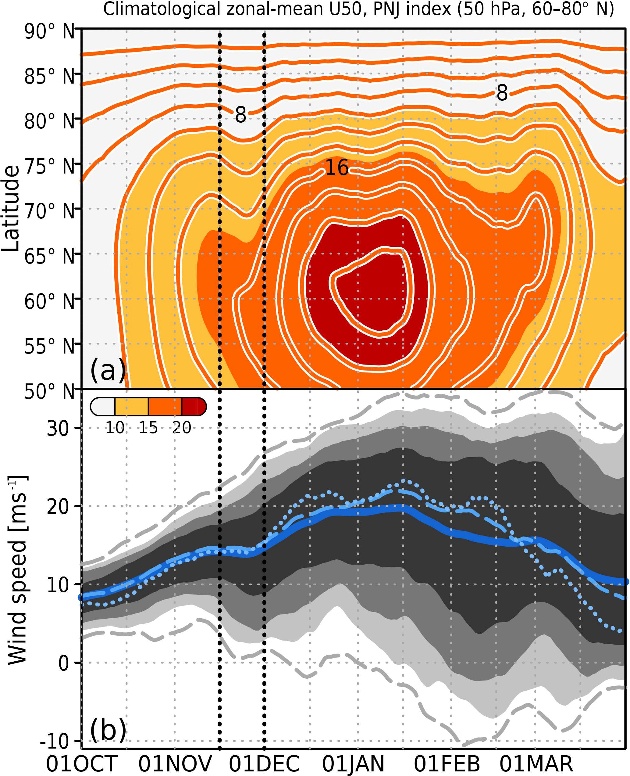
Figure 1(a) Latitude–time cross section of the 15-day running mean of the climatological zonal-mean zonal wind at 50 hPa (; lines and color shading) from 1 October through 31 March. The contour interval is 2.0 m s−1. (b) Time series of the climatological 15-day running mean of the PNJ index (m s−1, blue), defined as zonal-mean zonal wind speed at 60–80∘ N and 50 hPa. Dark gray shading indicates the 20th to 80th percentiles, medium gray shading indicates the 10th to 90th percentiles, and light gray shading indicates the 5th to 95th percentiles. The two gray dashed lines indicated the daily minimum and maximum of the PNJ. The blue dotted (dashed) line indicates the daily median (mode) of the PNJ. The vertical black dotted lines indicate the period of the short break in late November.
As our main analysis method, we performed an Eliassen–Palm (EP) flux analysis based on the transformed Eulerian mean (TEM) momentum equation (Eq. 3). This method, which is widely used in dynamic meteorology to diagnose wave and zonal-mean flow interaction, is described in detail as follows.
Eliassen–Palm flux analysis is widely used in dynamic meteorology to diagnose wave and zonal-mean flow interactions (e.g., Holton and Hakim, 2012; Vallis, 2017). The EP flux shows the propagation of Rossby (planetary) waves (Andrews and McIntyre, 1976). The meridional (Fϕ) and vertical (Fz) components of the EP flux (F) are defined as follows:
where a is the radius of the Earth, f is the Coriolis parameter, ϕ is latitude, θ is potential temperature, u is zonal wind, and v is meridional wind. Overbars denote zonal means, primes denote anomaly from the zonal mean, z is a log-pressure coordinate, and ρ0 is air density. is computed from the zonal mean of the potential temperature in log-pressure coordinates. The eddy-flux terms and are computed from the zonal anomalies in the 6-hourly data, and the product is zonally averaged and then time averaged to obtain 15-day means.
We used the primitive form of the transformed Eulerian mean momentum equation to examine the diagnostics of the zonal-mean momentum (e.g., Dunkerton et al., 1981; Andrews et al., 1987):
where and are the meridional and vertical components of the residual mean meridional circulation, and is a residual term that includes internal diffusion and surface friction as well as sub-grid-scale forcing such as gravity wave drag. Term A in Eq. (3) is the temporal tendency of the zonal-mean zonal wind, Term B is the Coriolis force acting on the residual mean meridional circulation and the meridional advection of zonal momentum, and Term C is the divergence of the EP flux vector, i.e., wave forcing.
The vertical component of the three-dimensional wave activity flux (WAF; Plumb, 1985) at 100 hPa provides a useful diagnostic for identifying the source region of vertically propagating stationary planetary waves. The zonal average of the WAF is the EP flux, so the vertical component of the WAF shows from where the wave propagates to the stratosphere. The eddy terms are computed from the zonal deviations relative to each 15-day mean (i.e., stationary wave component).
3.1 Climatological short break of the polar night jet
First, we outline the seasonal evolution of the PNJ. A latitude–time cross section of the zonal-mean zonal wind at 50 hPa over 50–90∘ N shows that the strength of the zonal-mean westerlies at 50 hPa ( increases with time from approximately October to late December. Subsequently, decreases with time from late December through March (Fig. 1a). An examination of the intraseasonal variation of reveals two short breaks. Between 60 and 80∘ N, there is a pause in the increasing trend in late November, and there is another pause in the decreasing trend in late February. The statistical significance of the short break in late November is described in Appendix B. The climatological short break in February is likely associated with the less frequent occurrence of SSWs in late February than in January and early February. We note the signal (the short break of the PNJ) throughout the whole stratosphere. In contrast, the climatological short break in November is restricted to the lower and mid-stratosphere (figure not shown).
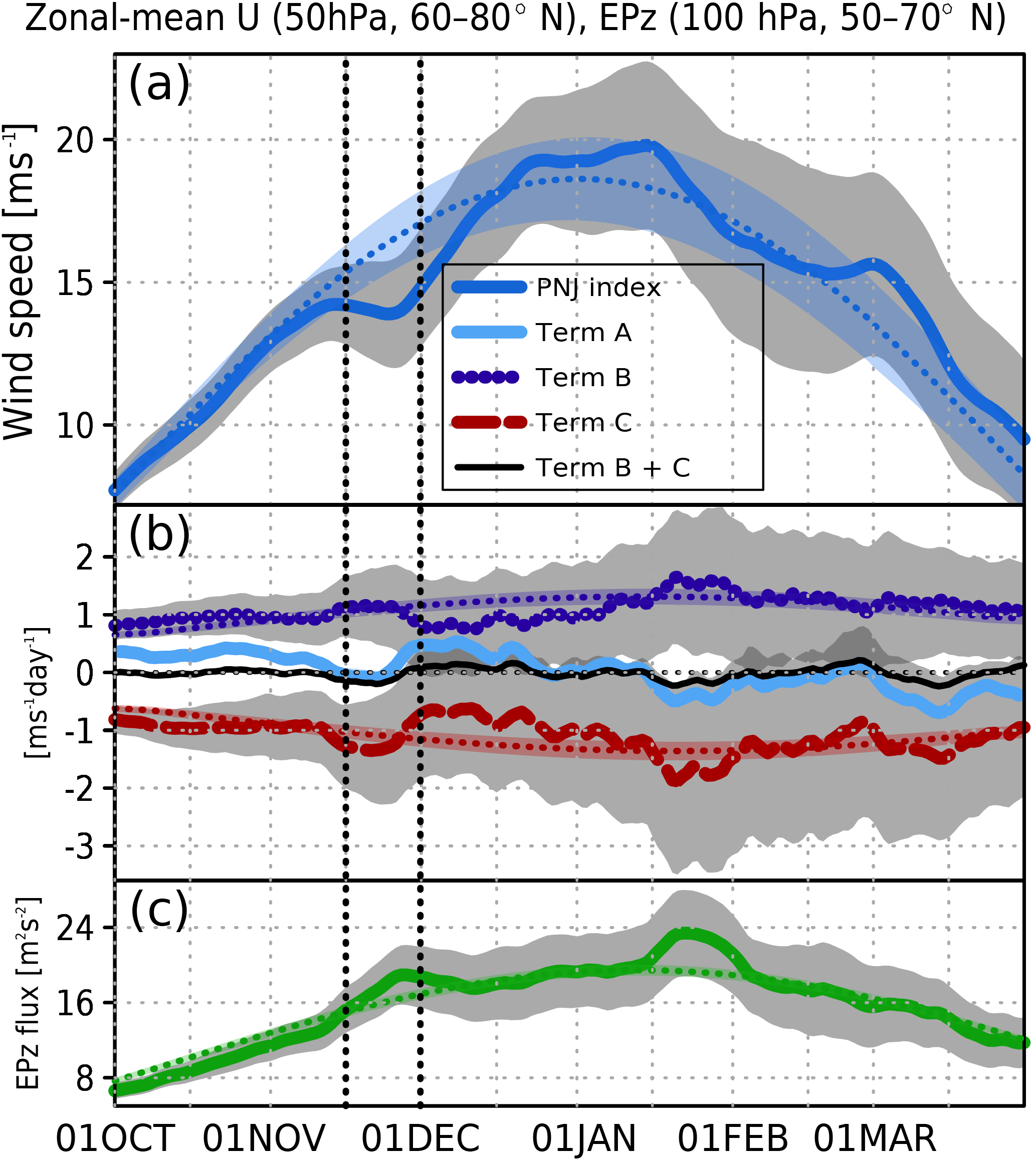
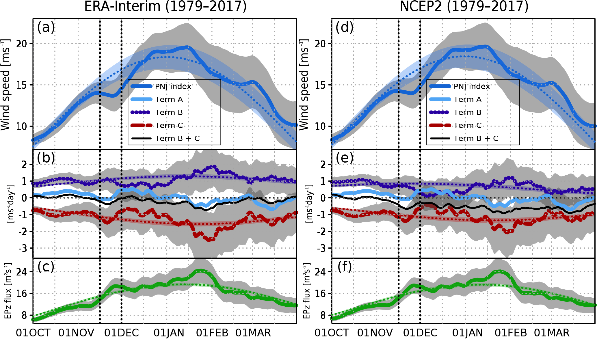
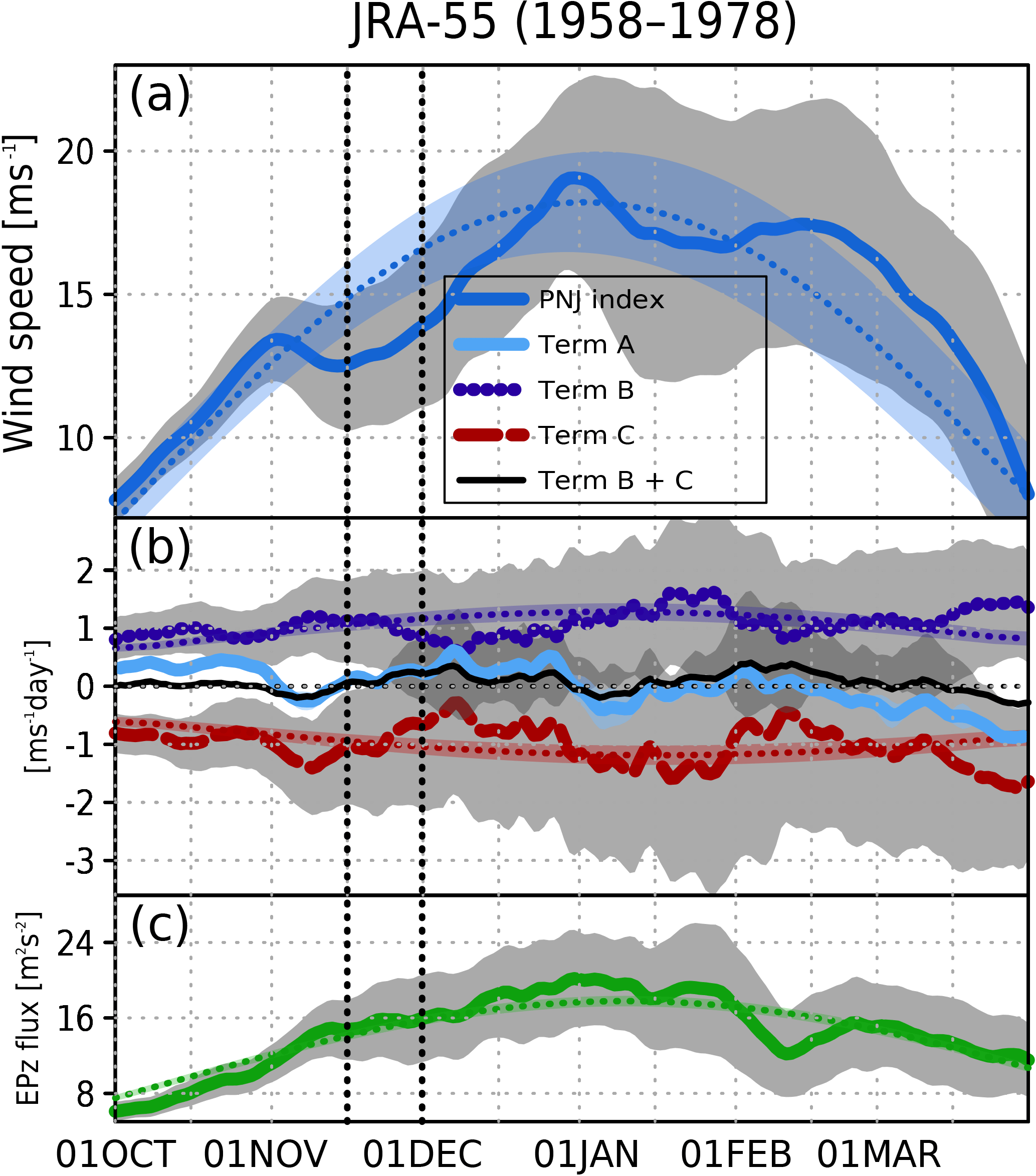
Figure 2Time series of climatological 15-day running means of the (a) PNJ index (m s−1, dark blue) (same as Fig. 1b); the sinusoidal regression expression of the PNJ index, dark blue dotted line); the 95 % confidence interval of the indices (color shading); (b) the temporal tendency of the PNJ (i.e., zonal acceleration (m s−1 day−1); Term A in Eq. 3, light blue line), the Coriolis force acting on the residual mean meridional circulation and the meridional advection of zonal momentum (m s−1 day−1, Term B in Eq. 3, purple line) at 50 hPa, and the EP flux divergence (m s−1 day−1, Term C in Eq. 3, red line) at 50 hPa averaged over latitudes 60–80∘ N; the sum of Term B and Term C (black line); the sinusoidal Term B (purple dotted line), and the sinusoidal Term C (red dotted line); the 95 % confidence interval of the indices (color shading); and (c) the vertical component of EP flux (Fz), the sinusoidal of the Fz (green dotted line), and the 95 % confidence interval of the indices (color shading) at 100 hPa (10−2 m2 s−2) averaged over latitudes 50–70∘ N from 1 October through 31 March. The vertical black dotted lines indicate the period of the late November short break.
Here, we defined the zonal-mean zonal wind speed at 60–80∘ N and 50 hPa as a PNJ index because the short break can be clearly seen in these latitudes (Fig. 1a). The time series of this PNJ index clearly shows a short break during late November (blue line in Fig. 1b). There are various bumps in the time series of a lower dashed–dotted line in Fig. 1b. This signifies that short breaks (SSWs) occur regardless of the time of the season; that is, the short breaks do not always occur in late November and early February in each year. The climatological (39-year average – this is the climatology in our definition) short break, however, occurs only during late November (blue line in Fig. 1b). This suggests that the short breaks in each year more often occur during late November than during the other periods, because the short break in late November is the only one that is statistically significant. We thus focus on the climatological short break in late November. The numbers of occurrence of the short break of the PNJ in late November is described in Appendix C.
3.2 Anomalous upward propagation of the EP flux during late November
In this section, we show that the late November climatological short break is caused by anomalous upward propagation of planetary waves. To investigate the dynamical cause of the short break in late November, we compared the time series of the PNJ index (Fig. 2a) with the intraseasonal variation of each term of the TEM equation (Eq. 3) (Fig. 2b). Here, Term A is the temporal tendency of the PNJ (i.e., its zonal acceleration); Term B is the Coriolis force acting on the residual mean meridional circulation and the meridional advection of zonal momentum; and Term C is the EP flux divergence at 50 hPa averaged over 60–70∘ N. The temporal tendency of the zonal wind accords well with the sum of the forcing terms of the TEM momentum diagnostic (A = B + C; Sect. 2.2; light blue and black lines in Fig. 2b). The EP flux divergence (wave forcing) generally governs the zonal wind tendency, and the short break in November is also caused by wave forcing (Term C in Eq. 3).
The vertical component of the EP flux (Fz) at 100 hPa, averaged over latitudes 50–70∘ N (Fig. 2c), is used as a measure of planetary-scale Rossby wave propagation into the stratosphere (e.g., Coy et al., 1997; Pawson and Naujokat, 1999; Newman et al., 2001). In late November, the upward EP flux at 100 hPa rapidly increases to its maximum, and this enhanced EP flux is linked to the EP flux convergence at 50 hPa, which brings about the short break.
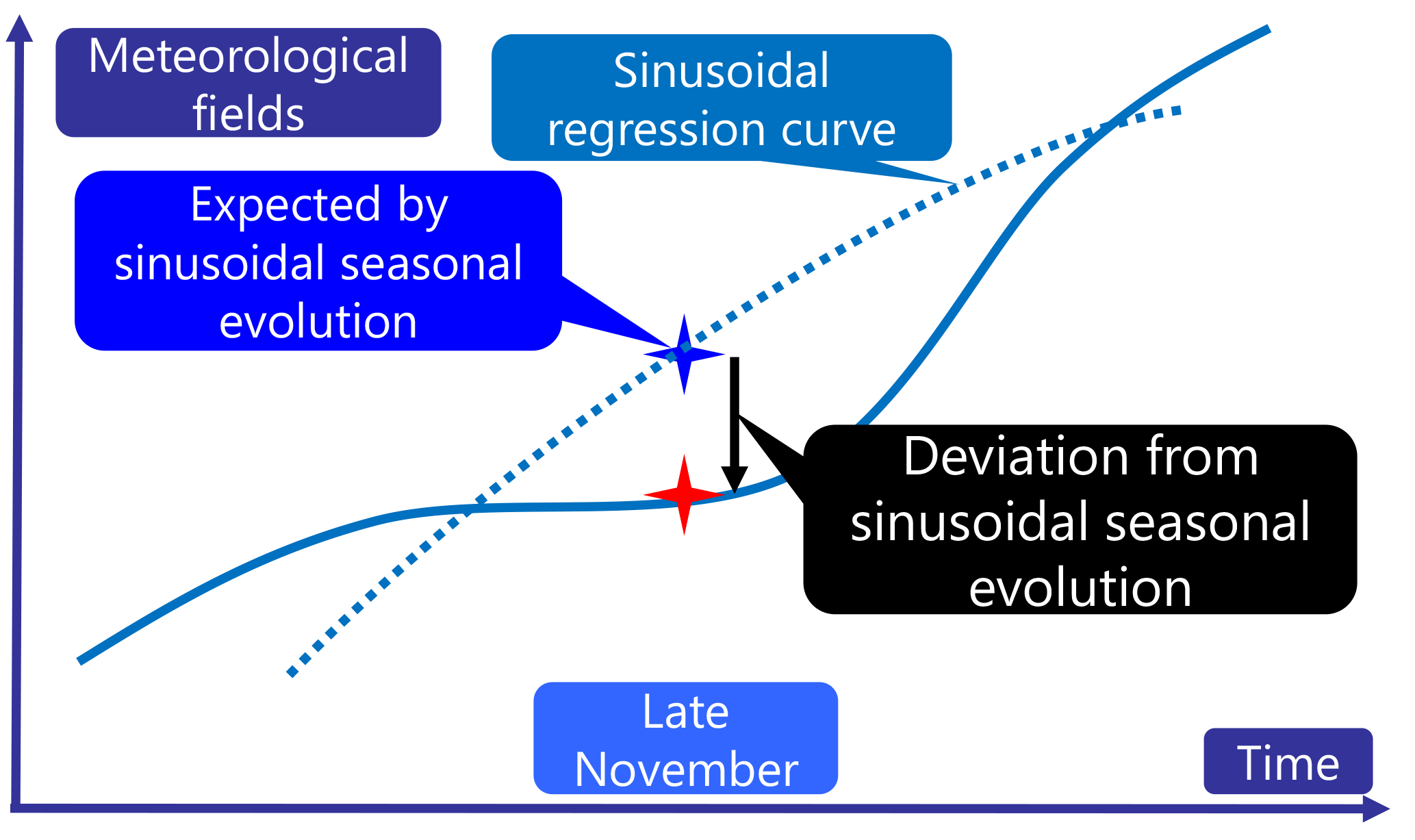
Figure 3Schematic diagram of a late November deviation in the seasonal evolution of a climatological meteorological field. Blue cross mark indicates the values of the meteorological field in late November expected by sinusoidal seasonal evolution, and the red cross mark indicates its actual value in late November. The vertical difference between the actual value (red cross mark) and the expected value (blue cross mark) during late November, which is calculated by Eq. (4), is the field deviation.
3.3 Calculation of anomalous fields with respect to a sinusoidal seasonal evolution in late November
We identified a period between 16 and 30 November for the late-November short break (see Fig. 1). We further defined a climatological meteorological field deviation, Adev, during the period of the short break as a deviation from the expected sinusoidal seasonal evolution (since that of solar forcing is sinusoidal, e.g., Andrews et al., 1987) of that field (Fig. 3):
where A is a climatological meteorological field (e.g., geopotential height) and subscripts indicate the averaging period. (sinusoidal regression expression of A16−30 Nov) is the expected climatological meteorological field during late November given a sinusoidal seasonal evolution (calculated by the average of regression analyses with the sinusoidal reference state in each year, 1 January to 31 December), and Adev is the deviation of the actual climatological meteorological field in late November from the expected field. All anomalous fields during the short break were calculated in this manner (see Figs. 4, D1d, D3d, D4d, D5d, D6d, D7, and E2). Many studies usually define anomaly fields as the ones from the climatological mean, but this paper does not define anomaly fields from the climatology. The anomaly field defined here is the actual climatological field minus the expected climatological field by the seasonal march. The dark blue dotted line in Fig. 3a shows the sinusoidal regression expression of the PNJ index. The short break is statistically significant at the 99.9 % confidence level (p=0.0003; the two-sided Wilcoxon signed-rank test for the differences of two dependent non-normality samples; late November and the expected value by sinusoidal seasonal evolution; e.g., Sheskin, 2011; Wilks, 2011). The bootstrap test of the short break in late November is described in Appendix B.
The meridional structures of the EP flux and zonal wind from November to early December are shown in Fig. D1a–c. Deviations of meteorological fields, that is, those that deviate from the expectation of a sinusoidal seasonal evolution (see Fig. 3), are also shown in Fig. D1d. An upward EP flux propagation deviation (vectors in Fig. D1d) is seen at 50–80∘ N from the upper troposphere (300 hPa) through the stratosphere (above 100 hPa). This flux deviation causes an EP flux convergence deviation in the high-latitude stratosphere (contours in Fig. D1d), which corresponds to the short break of the PNJ. This anomalous upward EP flux originates at mid- (40–60∘ N) and high latitudes (65–80∘ N). The detailed evolution of the EP flux and zonal wind from November to early December is described in Appendix D1. For reference, other climatological atmospheric fields from November to early December are described in Appendices D2, D3, D4, D5, and D6.
3.4 Links between the anomalous upward propagation of the EP flux and a tropospheric trough over eastern Siberia
This section shows that the anomalous (Term Adev in Eq. 4) upward propagation of planetary waves coincides with a deepening of the eastern Siberia trough (negative deviation of the geopotential height) in late November. To identify the specific area of the anomalous (Term Adev in Eq. 4) upward propagation of the EP flux during the period of the short break, we investigated the horizontal distribution of the (WAF). The largest positive deviation of the vertical component of the WAF of the stationary wave component at 100 hPa in late November is centered over Siberia and extends over most of the Eurasian continent (Fig. 4). This distribution implies that the Eurasian area is particularly important for stratosphere–troposphere coupling during late November.
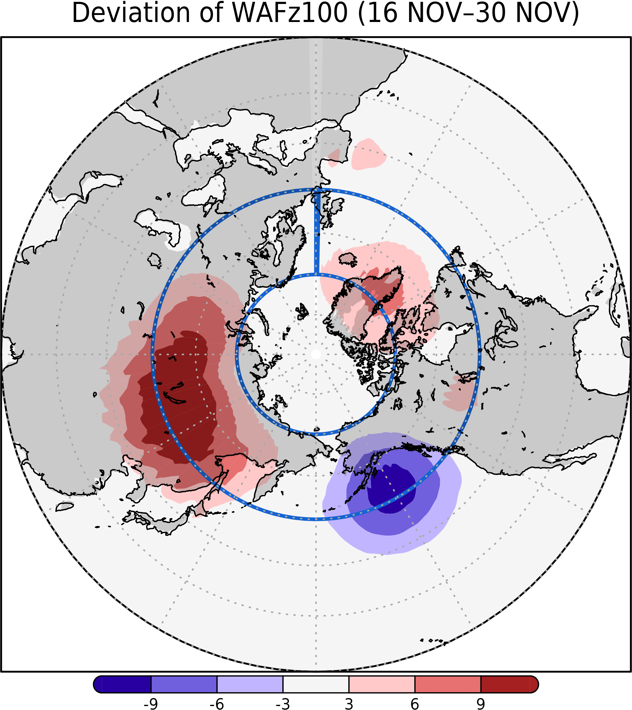
Figure 4Vertical component of the late November deviation of the climatological WAF (Plumb, 1985) at 100 hPa (10−3 m2 s−2) with respect to its sinusoidal seasonal evolution, calculated by Eq. (4) (see Sect. 3.3). The blue box (0–360∘ E, 50–70∘ N) indicates the averaging area used to calculate the fields shown in Fig. 2c.
During late November, the Rossby wave deviation propagates upward over central Siberia (60–100∘ E) in the lower troposphere and around east Siberia in the upper troposphere (Fig. D3d). The WAF divergence deviation is negative (figure not shown), indicating convergence in the stratosphere. We further examined the horizontal structure responsible for the upward WAF at 100 hPa. The vertical component is proportional to the meridional eddy heat flux (, where prime denotes the anomaly from the zonal mean). Over Siberia, the area of northerly wind and negative air temperature deviations (Fig. D4d) corresponds to the area of positive WAF deviations (Fig. 4). During late November, the trough over Siberia strengthens with time (see Fig. D3d). These results show that the anomalous (Term Adev in Eq. 4) upward propagation of planetary waves occurs simultaneously with the deepening of the eastern Siberia trough.
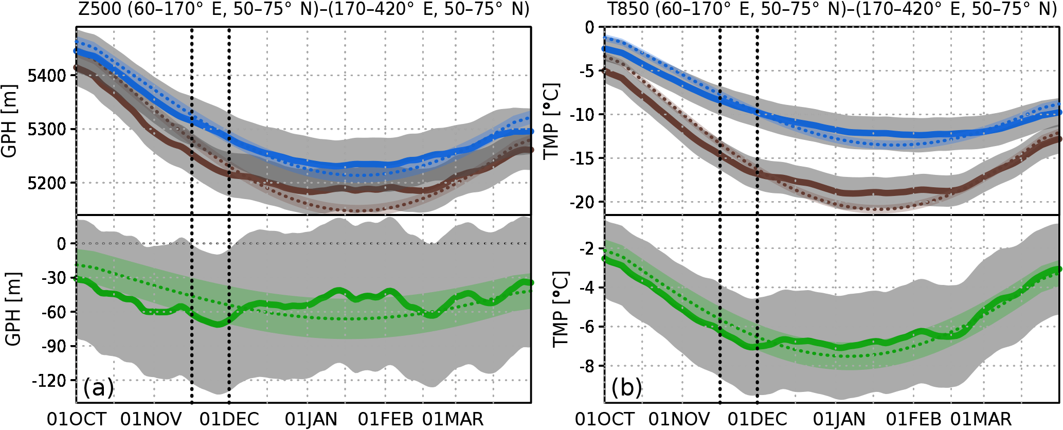
Figure 5Time series of the climatological 15-day running mean (a) Z500 (m) and (b) T850 (∘C) over Siberia (60–170∘ E, 50–75∘ N; brown lines), outside Siberia (170∘ E–60∘ W, 50–75∘ N; blue lines), and their anomalies within Siberia from their values outside of Siberia (green lines) from 1 October through 31 March. The dotted lines are sinusoidal lines, and color shadings indicate a 95 % confidence interval. The vertical black dotted lines indicate the period of the late November short break.
3.5 Geopotential height and air temperature in the middle troposphere
In Sect. 3.4, we showed that the deepening of the trough over Siberia is associated with the strengthening the anomalous (Term Adev in Eq. 4) vertical propagation of planetary waves and the occurrence of the short break. In this section, we show that the deepening of the eastern Siberia trough is associated with geopotential height and air temperature deviations. It is generally known that Rossby waves that propagate into the stratosphere in the high latitudes are planetary-scale waves with wavenumbers 1 to 2 (e.g., Baldwin and Dunkerton, 1999). Here, to identify the source of the deviations, we consider the planetary-scale wave components (i.e., wavenumbers 1 to 2) of geopotential height and air temperature in the troposphere. During late November, deviations of eddy geopotential height at 500 hPa (Z500) are strongly negative over Siberia, whereas they are strongly positive over the Atlantic Ocean (Fig. D5d). This positive–negative contrast means that the trough over Siberia is strengthened and the planetary-scale eddy at Z500 is amplified at high latitudes. Cold deviations of eddy air temperature at 850 hPa (T850) are also seen over Siberia along the Arctic Ocean coast (Fig. D6d), west of the negative geopotential deviation (Fig. D5d). The area of these cold deviations is included in the northerly wind deviation area. Where these areas coincide, the eddy meridional heat flux ( is enhanced. A similar but small enhancement of is also seen over Greenland, where a positive T deviation is observed (Fig. D6d), and over the North Atlantic Ocean, where a positive geopotential deviation is observed (Fig. D5d). The vertical component of the WAF with wave planetary-scale components is described in Appendix D6.
Why does the atmospheric trough strengthen over Siberia at this time of the year? We hypothesize that a high-latitude land–sea thermal contrast strengthens the trough. Figure 5 shows the time series of Z500 and T850 over Siberia (60–170∘ E, 50–75∘ N; inside the brown box in Figs. D5 and D6) and outside of Siberia (170∘ E–60∘ W, 50–70∘ N; inside the blue box in Figs. D5 and D6). The time series of the differences between inside and outside of Siberia (green lines) are also shown. During late November, the rate of increase in the zonal contrast (wave amplitude) of Z500 reaches a maximum (green line in Fig. 5a). Similarly, the rate of increase in the zonal T850 contrast, which roughly corresponds to a high-latitude land–sea thermal contrast, approaches a maximum during late November (green line in Fig. 5b). Siberia is of course a land region, whereas the area outside of Siberia is occupied mainly by oceans, in particular, the North Atlantic Ocean. Moreover, increased snow cover over eastern Siberia can contribute to the enhancement of the radiative cooling and subsequent formation of a surface inversion layer. The surface inversion starts to form in early November. Strong radiative cooling within the inversion layer possibly sustains extremely low air temperature at the ground level (Iijma and Hori, 2016). Therefore, we hypothesize that thermal forcing due to the land–sea contrast results in the amplification of the trough over Siberia. It is generally known that there are three main sources of the stationary waves that are responsible for zonally asymmetric circulation in the NH: a land–sea thermal contrast, large-scale orography, and tropical diabatic heating (e.g., Smagorinsky, 1953; Inatsu et al., 2002). Large-scale orography (in the NH, the Himalayas, and Rockies in particular) has been found by many studies to be an important source of planetary waves (e.g., Held et al., 2002; Chang, 2009; Saulière et al., 2012). We demonstrated here that the source of the planetary wave in the troposphere during late November is at higher latitude than the Himalayas (see Figs. 4, D5d, and D6d). Strengthening of the high-latitude land–sea thermal contrast may mainly account for the short break in the PNJ during late November. We did not find any short breaks in the Southern Hemisphere (figure not shown). The absence of a short break in the Southern Hemisphere is logically consistent with our hypothesis, because there are no high-latitude zonal land–sea thermal contrasts there.
Some studies have described that the PNJ variations are related to the quasi-biennial oscillation (QBO; Baldwin et al., 2001) (e.g., Holton and Tan, 1980, 1982; Gray et al., 2003; Anstey and Shepherd, 2014). This might also affect the short break and is discussed in detail in Appendix E. The seasonal evolution from easterly to westerly winds in the stratosphere is a highly nonlinear transformation in terms of the ability for waves to propagate into the stratosphere (Plumb, 1989). A hidden alternative mechanism may control the short break, but it is out of the scope of the present study.
We detected a short break in the seasonal evolution of climatological PNJ during late November (see Fig. 1). Examination of the atmospheric dynamical balance showed that an increase in upward propagation of planetary waves from the troposphere to the stratosphere in late November is accompanied by convergence of the EP flux in the stratosphere, which brings about this short break in the PNJ (see Fig. 2). The upward propagation of Rossby (planetary) waves over Siberia from the troposphere to the stratosphere is a dominant cause of the short break (see Fig. 4). This upward propagation of planetary-scale Rossby waves at high latitudes is associated with amplification of eddy geopotential height and air temperature, that is, with a strengthening of the trough over Siberia. Further, we inferred that this strengthening of the trough is forced by the high-latitude land–sea thermal contrast around Siberia (see Fig. 5). Influence of the November short break upon tropospheric extreme weather and climate remains to be examined.
The Grid Analysis and Display System (GrADS) version 2.2.1 (http://cola.gmu.edu/grads, last access: 20 August 2018) and the Generic Mapping Tools (GMT) version 5.4.4 (http://gmt.soest.hawaii.edu/, last access: 20 August 2018) were used to draw the figures.
All analyses performed in this study were based on data publicly available, as described in Sect. 2.1 and Appendix A.
For reference, we used other datasets – ERA-Interim with the 1.5∘ horizontal resolution (available from the web page http://apps.ecmwf.int/datasets, last access: 20 August 2018) (Dee et al., 2011) and NCEP/DOE Reanalysis 2 (NCEP2) with 2.5∘ horizontal resolution (available from the web page https://www.esrl.noaa.gov/psd/data/gridded/data.ncep.reanalysis2.html, last access: 20 August 2018) (Kanamitsu et al., 2002). Figure A1 is the same as Fig. 2, but (a)–(c) used ERA-Interim and (d)–(f) used NCEP2 (39-year average during 1979–2017). The seasonal evolution of the PNJ index is almost same, including the short break of the PNJ in late November. We used JRA-55 with analysis period 1958–1978, before the inclusion of satellite data. Figure A2 is the same as Fig. 2, but for the 21-year average during 1958–1978. The short break of the PNJ is in early November, not in late November.
We investigated two kinds of a statistical test for the short break of the PNJ. The short break was statistically significant at the 99 % confidence level in two ways. The first method is a test for differences of two samples. The second is a two-sample bootstrap test.
B1 Test for differences of two samples
We defined three samples and the differences of the PNJ of two continuous 15-day mean periods in same year: (a) early November and late October, (b) late and early November, and (c) early December and late November. If the short break in late November is statistically significant, sample (b) is significantly different than samples (a) or (c).
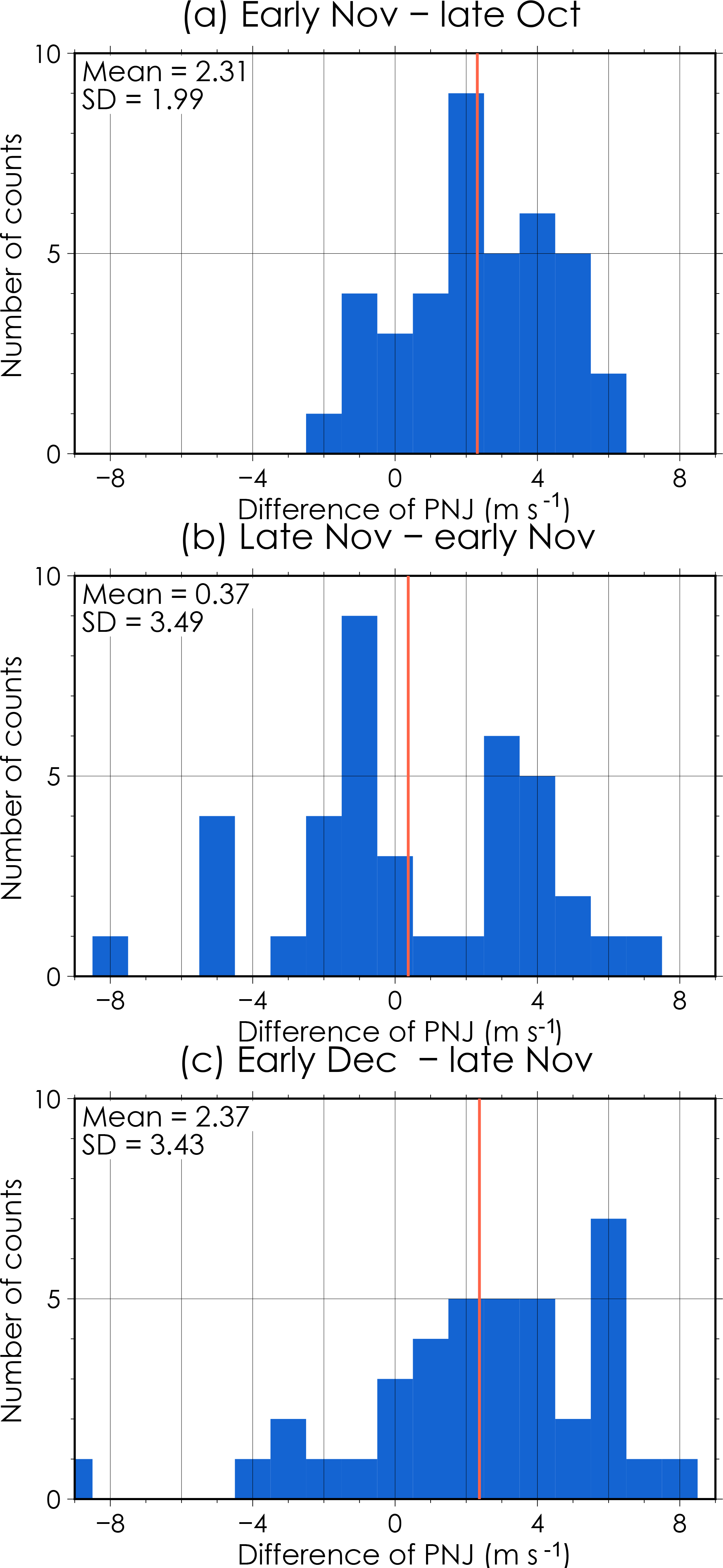
Figure B1Histograms of the difference of the PNJ in (a) early November and late October, (b) late and early November, and (c) early December and late November (1.0 m s−1 bins). The vertical axis indicates the number of counts for each bin. The labels on the upper-left corner show the mean and standard deviation. The orange lines indicate the mean.
Figure B1 shows histograms of samples (a), (b), and (c). These histograms seem to be different forms and variances. The test for differences has several ways depending on whether the samples follow a normal distribution and are of equal variances. We first calculated a test for normality. Second, we investigated a test for equality of two variances. We finally calculated a test for differences of two samples in appropriate ways.
First, we calculated a Shapiro–Wilk test for normality (Shapiro and Wilk, 1965). The null hypothesis for this test is that the data are normally distributed. The data that followed a normal distribution are those of samples (a) (the null hypothesis was not rejected; p=0.857) and (b) (p=0.331); the data of sample (c) did not follow a normal distribution (the null hypothesis was rejected at the 95 % confidence level; p=0.021). We then investigated an F test for two population variances. The differences of the variances are not statistically significant in samples (b) and (c) (p=0.92), but they are statistically significant in samples (a) and (b) (99 % confidence level; p=0.001) and in samples (a) and (c) (99 % confidence level; p=0.001). Finally, we calculated a statistical test for the differences of two samples. The differences of populations are statistically significant in samples (a) and (b) at the 99 % confidence level (p=0.004; Welch's t test, Welch, 1947; assumption of normality and unequal variances) and in samples (b) and (c) at the 99 % confidence level (p=0.008; Mann–Whitney U test, Mann and Whitney, 1947; assumption of non-normality and equal variances); however, they are not statistically significant in samples (a) and (c) (p=0.493; Brunner–Munzel test, Brunner and Munzel, 2000; assumption of non-normality and unequal variances). Thus, sample (b) (the difference of late and early November) was only statistically significantly different from other samples at the 99 % confidence level.
B2 Two-sample bootstrap test
We tried a two-sample bootstrap test (e.g., Sheskin, 2011; Wilks, 2011) as follows: resampling with replacement from the 39 available years (giving 10 000 different 39-year composites). One sample is the observed PNJ in late November, and the other is the expected PNJ by sinusoidal seasonal evolution. The null hypothesis is that difference between the two bootstrap samples is equal to zero. The difference was statistically significant at the 99 % confidence level (p=0.006).
We investigated in how many winters the short break appears. The definition of the occurrence of the short break was the year when the deviation of the PNJ in late November from the one expected by sinusoidal seasonal evolution was negative. The number of the negative years were 27 years (relative frequency is 0.69) (Fig. C1). The mean is −2.11, and the 95 % confidence interval of the mean is −3.29 to −0.93.

Figure C1Histogram of the deviation of the PNJ in late November from the expected by sinusoidal seasonal evolution in each year (2.0 m s−1 bins). The horizontal axis shows the deviation for the center of each bin. The vertical axis indicates the number of counts for each bin. The labels on the upper-left corner show the mean and standard deviation. The orange lines indicate the mean. The negative sign indicates the occurrence of the short break.
D1 Zonal-mean zonal wind, EP flux, and EP flux divergence
Figure D1a–c shows the climatological zonal-mean zonal wind, EP flux, and EP flux divergence in the NH during (a) early November, (b) late November, and (c) early December. The subtropical jet is commonly centered in the upper troposphere at 35∘ N, 200 hPa, and the PNJ is centered in the stratosphere at 65∘ N. These two westerly maxima gradually strengthen with time. The EP flux propagates upward from the lower troposphere to the mid- and upper troposphere in the low latitudes, and it propagates into the stratosphere in the high latitudes. The EP flux also gradually propagates upward with time. Figure D1d shows the departures of the fields shown in Fig. D1b from the sinusoidal evolution of the fields shown Fig. D1a and c (calculated by Eq. 4). Thus, Fig. D1d shows the late November field deviations from a sinusoidal seasonal evolution.
D2 Vertical component of the wave activity flux of the stationary wave component at 100 hPa
Figure D2a–c shows the vertical component of the climatological wave activity flux (WAF) of the stationary wave component at 100 hPa during early November, late November, and early December, respectively. During all three periods, a strong positive signature is centered in the Russian far east and extends from eastern Europe to the east coast of Asia.
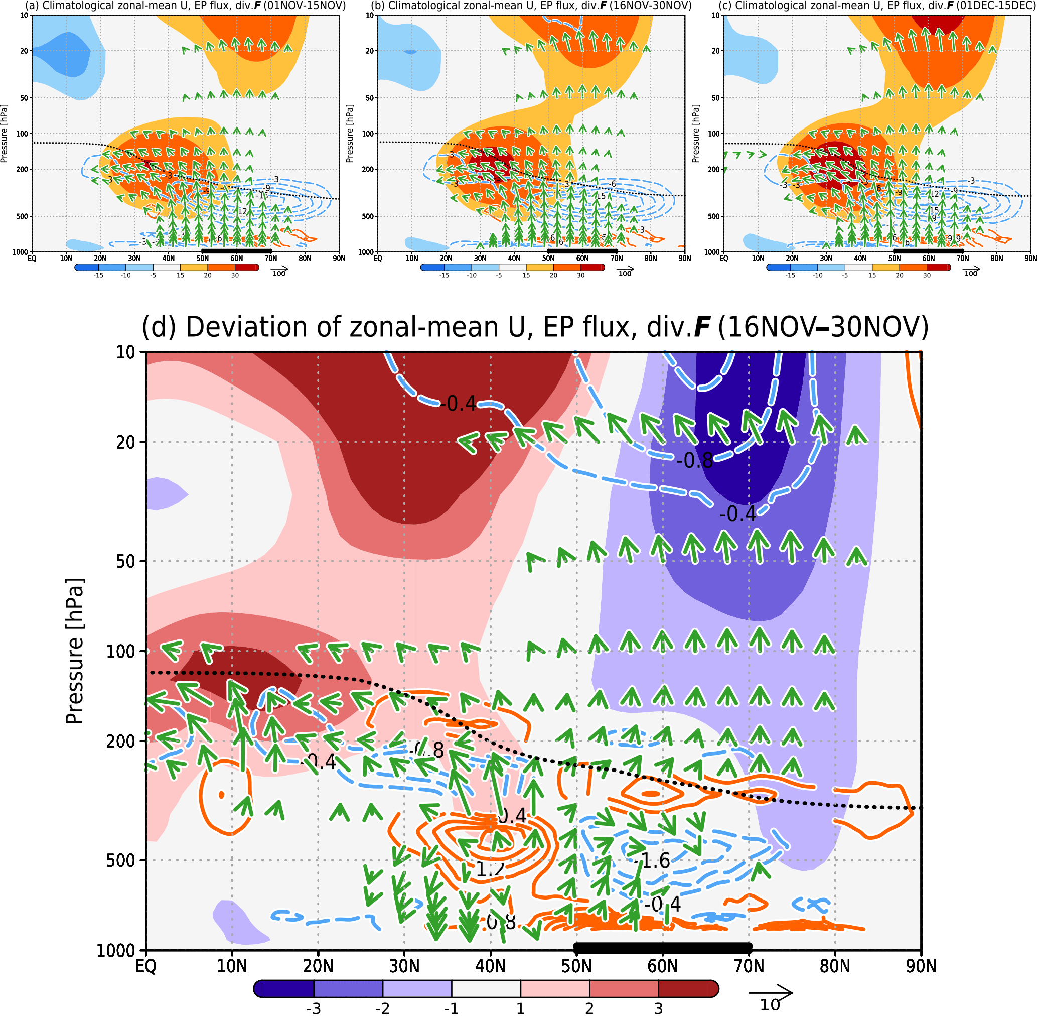
Figure D1Climatological zonal-mean zonal wind speed (m s−1, color shading), EP flux (m2 s−2, vectors), and the flux divergence (m s−1 day−1, contours) during (a) early November (1–15 November), (b) late November (16–30 November), and (c) early December (1–15 December). (d) Late November deviations from the expected sinusoidal regression expression calculated with Eq. 4 (see Sect. 3.3). The EP flux is standardized by density (1.225 kg m−3) and the radius of the Earth (6.37×10⁶ m). The vertical component of the vectors is multiplied by a factor of 250. The bold black line indicates the longitudinal range for Siberia (50–70∘ N). The black dashed line indicates the tropopause height during these periods defined by WMO (1957). The definition is the lowest height at which the temperature lapse rate decreases to 2 K km−1 or less and remains below this value for a depth of at least 2 km.

Figure D2Vertical component of the climatological wave activity flux (Plumb, 1985) at 100 hPa (10−3 m2 s−2) during (a) early November, (b) late November, and (c) early December. The box outlined in blue (0–360∘ E, 50–70∘ N) indicates the averaging area used for calculating the fields shown in Fig. D3.
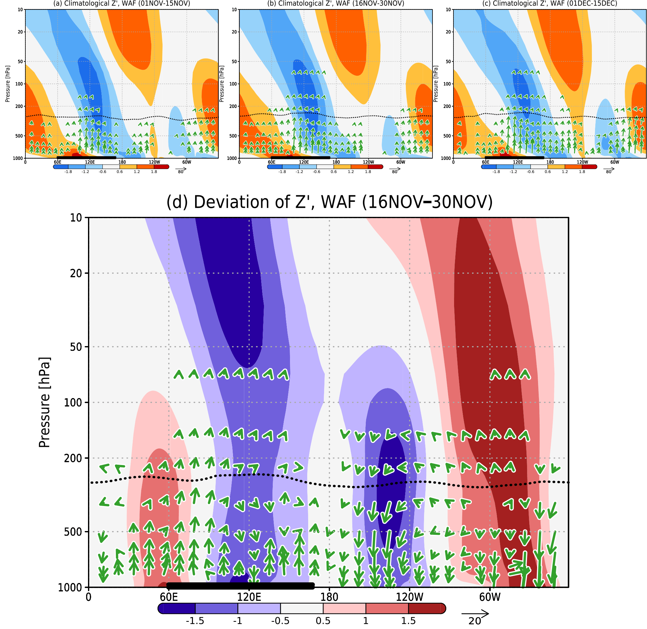
Figure D3Zonal anomalies of climatological geopotential height (m, color shading) and zonal and vertical components of WAF (10−3 m2 s−2, vectors), averaged over latitude 50–70∘ N (inside the blue box in Fig. A2) during (a) early November, (b) late November, and (c) early December. (d) late November field deviations calculated by Eq. (4) (see Sect. 3.3). The geopotential height is normalized by the standard deviation at each height. The WAF magnitude is standardized by pressure (p , ps is a standard sea level pressure) and the square of the radius of the Earth (6.37×10⁶ m). The vertical components of the vectors are multiplied by a factor of 500. The black line indicates the latitudinal range for Siberia (60–170∘ E). The black dashed line indicates the tropopause height defined by WMO (1957).
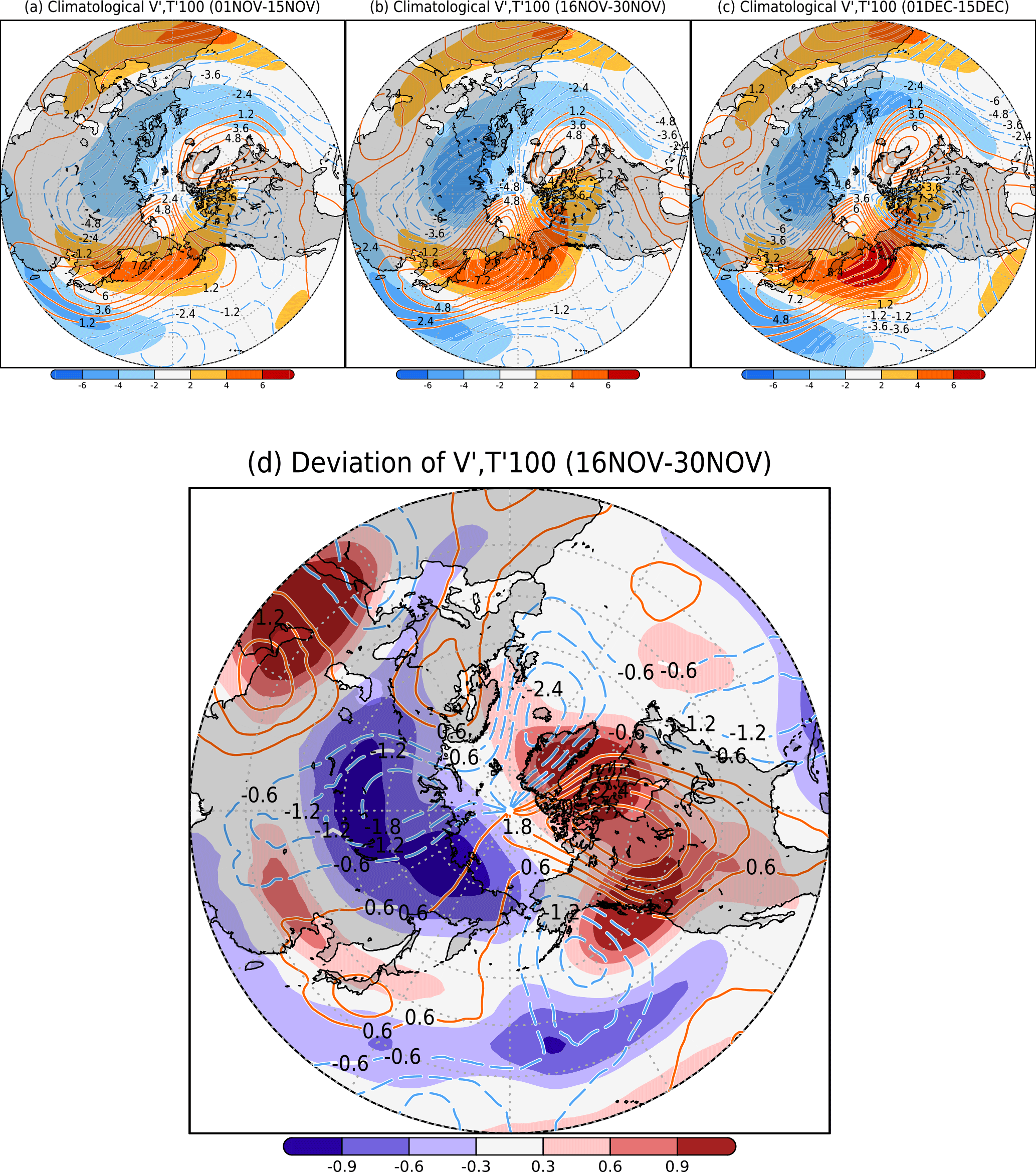
Figure D4Zonal anomalies of climatological meridional wind (m s−1, contours) and air temperature (∘C, color shading) at 100 hPa during (a) early November, (b) late November, and (c) early December. (d) Late November deviations calculated by Eq. (4) (see Sect. 3.3).
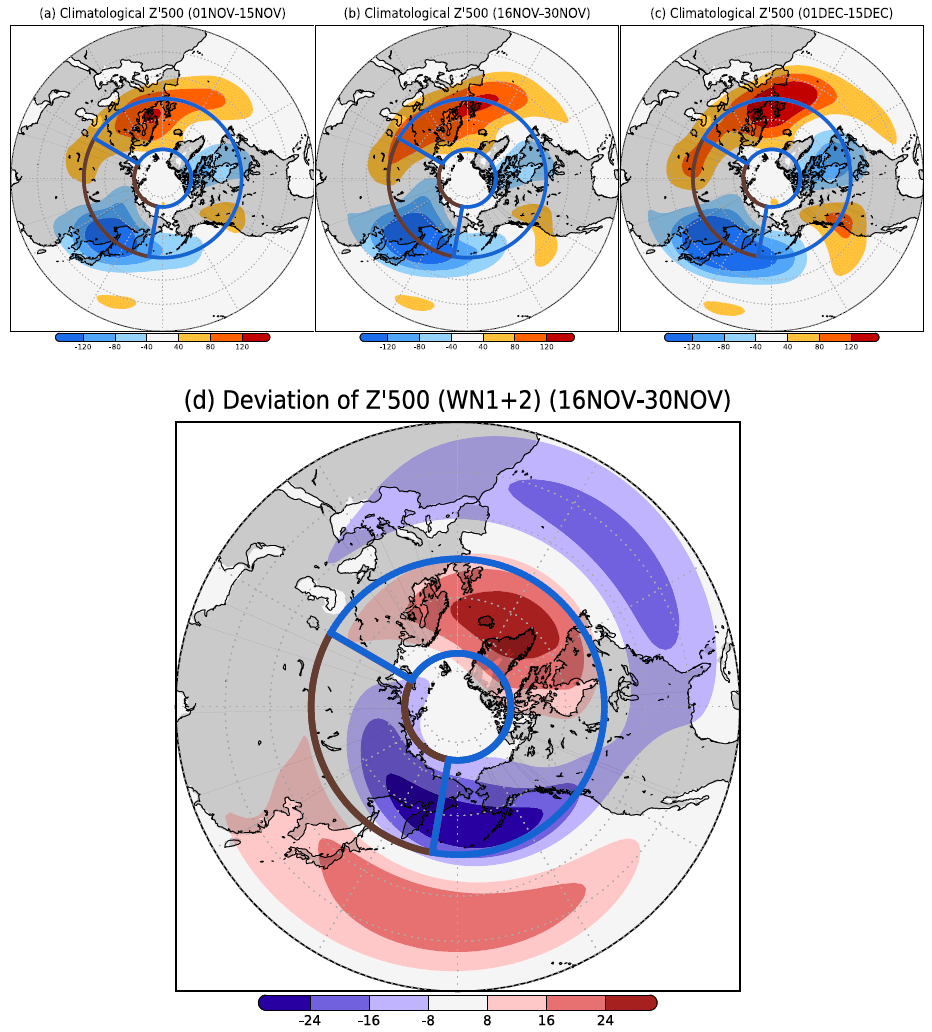
Figure D5Zonal anomalies of climatological geopotential height at 500 hPa (m) during (a) early November, (b) late November, and (c) early December. (d) Late November deviations calculated by Eq. (4) (see Sect. 3.3) with wavenumber decomposition; only planetary-scale components, wavenumbers 1 to 2, were used. The brown (60–170∘ E, 50–75∘ N) and blue (170∘ E–60∘ W, 50–75∘ N) boxes indicate the averaging areas used for calculating the fields shown in Fig. 5.

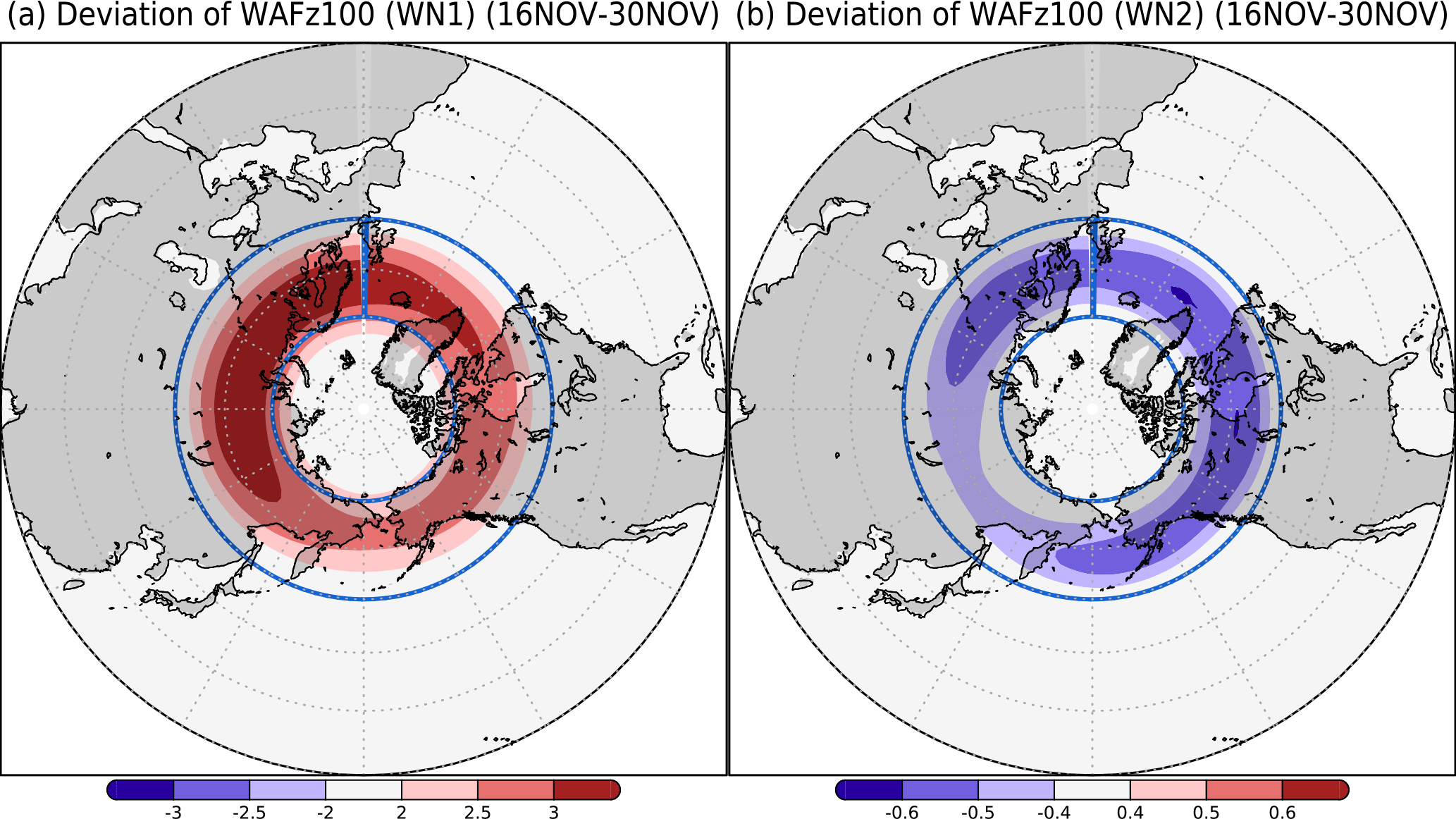
Figure D7Same as Fig. 4, but with wavenumber decomposition: (a) wavenumber 1 and (b) wavenumber 2.
Eddy component of geopotential height and zonal and vertical components of the WAF averaged over 50–70∘ N
Figure D3a–c shows the eddies (anomalies from the zonal mean) of climatological geopotential height and the zonal and vertical components of the climatological WAF distribution, averaged over 50–70∘ N (inside the blue box in Fig. D2) during early November, late November, and early December, respectively. Over east Siberia (100–120∘ E), an area of strong negative eddies (i.e., a geopotential height trough) extends from the middle troposphere to the stratosphere with a westward–upward tilt, and an area of positive eddies (i.e., a ridge) occurs near the surface over east Siberia (i.e., the area of Siberian High). Over 180∘ E–120∘ W, there is an area of strong positive anomalies in the stratosphere (i.e., the Aleutian High). Rossby waves propagate upward over east Siberia from the lower troposphere to the upper troposphere. Figure D3d shows the late November deviations. Note that the WAF was calculated with Eq. (4), not from the zonal anomalies of climatological geopotential height shown in Fig. D3d.
D4 Zonal anomalies of meridional wind and air temperature at 100 hPa
Figure D4a–c shows the zonal anomalies of climatological meridional wind and air temperature at 100 hPa during early November, late November, and early December, respectively. During all three periods, northerly winds and negative air temperatures occur over Siberia and southerly winds and positive air temperatures occur over the northwest Pacific Ocean. This collocation corresponds to the area of positive anomalies of the WAF over Siberia (see Fig. D2a–c). Figure D4d shows the zonal anomalies of meridional wind and air temperature deviations at 100 hPa.
D5 Geopotential height and air temperature in middle troposphere
Figure D5a–c shows the climatological eddy geopotential height at 500 hPa (Z500) during early November, late November, and early December, respectively. Negative anomalies (trough) are seen from east Siberia to East Asia, whereas positive anomalies (ridge) are over the North Atlantic Ocean to Europe. Figure D5d shows the planetary-scale eddy geopotential height deviation at 500 hPa. Figure D6 is the same as Fig. D5, but for air temperature at 850 hPa (T850). Negative anomalies (cold air) are seen over east Siberia to East Asia, and positive anomalies (warm air) are apparent over the North Atlantic Ocean to Europe (Fig. D6a–c).
D6 The anomalous upward propagation of the WAF with wavenumber decomposition
The WAF at 100 hPa is only very weakly correlated with anomalies within the troposphere, especially on sub-monthly timescales (Fig. 15 in de la Cámara et al., 2017). A big reason is that the planetary-scale waves that propagate into the stratosphere are dwarfed by the WAF variability associated with waves that are trapped with the troposphere. We therefore consider the planetary-scale wave components (wavenumbers 1 to 2) of the WAF. Figure D7 shows the same as Fig. 4, but with wavenumber decomposition, (a) wavenumber 1 and (b) that of wavenumber 2. The large positive deviation of the WAF with wavenumber 1 is centered over high-latitude Eurasia (Fig. D7a). However, the negative deviation of the WAF with wavenumber 2 is also centered over Eurasia (Fig. D7b). Thus, the WAF with wavenumber 1 contributed to the positive deviation.
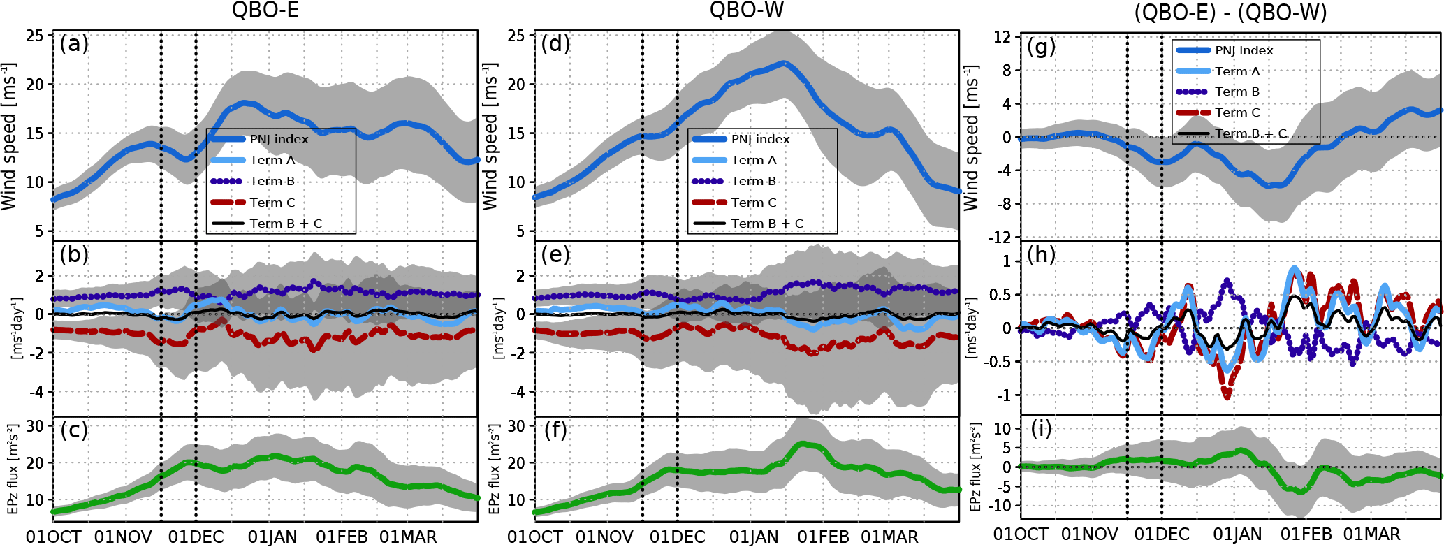
Figure E1Same as Fig. 2, but (a)–(c) for QBO-E, (d)–(f) for QBO-W, and (g)–(i) the difference between QBO-E and QBO-W.
Some studies have described that the PNJ variations are related to a quasi-biennial oscillation (QBO; Baldwin et al., 2001) (e.g., Holton and Tan, 1980, 1982; Labitzke, 1987; Gray et al., 2003; Anstey and Shepherd 2014). The PNJ is anomalously weak during the easterly phase of the QBO (QBO-E), whereas the PNJ is anomalously strong in the westerly phase of the QBO (QBO-W) in late winter. We compared the difference between the composite average in the years of the QBO-E and that of the QBO-W. The QBO-E and the QBO-W are defined as the direction of the zonal-mean zonal wind at 50 hPa averaged over 10∘ S–10∘ N in November. The number of years of the QBO-E is 16 years (1979, 1981, 1984, 1989, 1991, 1992, 1994, 1996, 1998, 2000, 2001, 2003, 2005, 2007, 2012, 2014). The number of years of the QBO-W is 23 years (1980, 1982, 1983, 1985, 1986, 1987, 1988, 1990, 1993, 1995, 1997, 1999, 2002, 2004, 2006, 2008, 2009, 2010, 2011, 2013, 2015, 2016, 2017). The short breaks occur during late November in both years. The PNJ in the QBO-E has a clearer short break and is weaker than in the QBO-W (Figs. E1 and E2). However, the difference is not statistically significant.
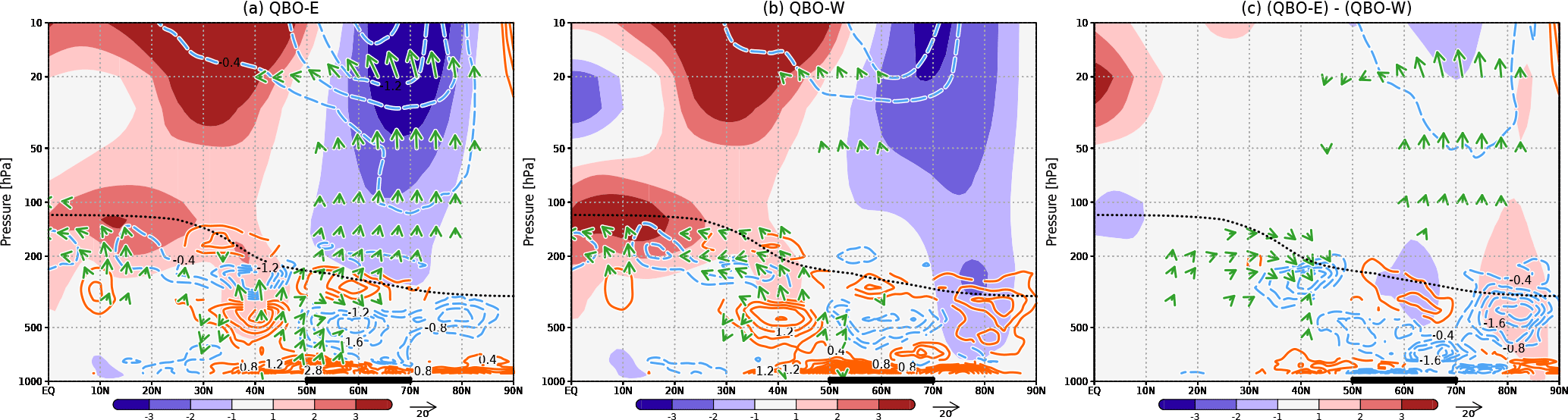
Figure E2Same as Fig. D1d, but (a) for QBO-E, (b) for QBO-W, and (c) the difference between QBO-E and QBO-W. The black dashed line indicates the tropopause height defined by WMO (1957).
YA initially focused on the short break of the PNJ. YA, KY, YT, MO, and JU analyzed the data. Moreover, mainly KY and JU investigated the statistical tests. YA and YT prepared the manuscript with contributions from all co-authors.
The authors declare that they have no conflict of interest.
We deeply thank Kunihiko Kodera for very insightful discussions. Advice and
comments given by Yasuhisa Kuzuha and Yoshihiro Iijima have been a great help
in the paper. Students in the Weather and Climate Dynamics Division offered
us fruitful advice. Suggestions by the two anonymous reviewers and Gloria
Manney helped us to improve the paper. This study was supported by the
Ministry of Education, Culture, Sports, Science and Technology (MEXT) through
a Grant-in-Aid for Scientific Research on Innovative Areas (grant number
22106003); the Green Network of Excellence (GRENE) Arctic Climate
Change Research Project; the Arctic Challenge for Sustainability (ArCS)
Project; and Belmont Forum InterDec Project. The work of Masayo Ogi was
supported by the Canada Excellence Research Chairs (CERC) Program.
Edited by: Amanda Maycock
Reviewed by: two anonymous referees
Ambaum, M. H. P. and Hoskins, B. J.: The NAO troposphere-stratosphere connection, J. Climate, 15, 1969–1978, https://doi.org/10.1175/1520-0442(2002)015<1969:TNTSC>2.0.CO;2, 2002.
AMS: Polar vortex, Glossary of Meteorology, available at: http://glossary.ametsoc.org/wiki/polar_vortex (ast access: 20 August 2018), 2015.
Ando, Y., Ogi, M., and Tachibana, Y.: Abnormal Winter Weather in Japan during 2012 Controlled by Large-Scale Atmospheric and Small-Scale Oceanic Phenomena, Mon. Weather Rev., 143, 54–63, https://doi.org/10.1175/MWR-D-14-00032.1, 2015.
Andrews, D. G. and McIntyre, M. E.: Planetary Waves in Horizontal and Vertical Shear: The Generalized Eliassen–Palm Relation and the Mean Zonal Acceleration, J. Atmos. Sci., 33, 2031–2048, https://doi.org/10.1175/1520-0469(1976)033<2031:PWIHAV>2.0.CO;2, 1976.
Andrews, D. G., Holton, J. R., and Leovy, C. B.: Middle Atmosphere Dynamics, Academic Press, San Diego, CA, USA, 1987.
Angell, J. K.: Changes in the 300-mb north circumpolar vortex, 1963–2001, J. Climate, 19, 2984–2995, https://doi.org/10.1175/JCLI3778.1, 2006.
Anstey, J. A. and Shepherd, T. G.: High-latitude influence of the quasi-biennial oscillation, Q. J. Roy. Meteor. Soc., 140, 1–21, https://doi.org/10.1002/qj.2132, 2014.
Baldwin, M. P. and Dunkerton, T. J.: Propagation of the Arctic Oscillation from the stratosphere to the troposphere, J. Geophys. Res.-Atmos., 104, 30937–30946, https://doi.org/10.1029/1999JD900445, 1999.
Baldwin, M. P. and Dunkerton, T. J.: Stratospheric harbingers of anomalous weather regimes, Science, 294, 581–584, https://doi.org/10.1126/science.1063315, 2001.
Baldwin, M. P., Gray, L. J., Dunkerton, T. J., Hamilton, K., Haynes, P. H., Randel, W. J., Holton, J. R., Alexander, M. J., Hirota, I., Horinouchi, T., Jones, D. B. A., Kinnersley, J. S., Marquardt, C., Sato, K., and Takahashi, M.: The quasi-biennial oscillation, Rev. Geophys., 39, 179–229, https://doi.org/10.1029/1999RG000073, 2001.
Black, R. X. and McDaniel, B. A.: Submonthly Polar Vortex Variability and Stratosphere–Troposphere Coupling in the Arctic, J. Climate, 22, 5886–5901, https://doi.org/10.1175/2009JCLI2730.1, 2009.
Brasefield, C. J.: Winds and temperatures in the lower stratosphere, J. Meteorol., 7, 66–69, https://doi.org/10.1175/1520-0469(1950)007<0066:WATITL>2.0.CO;2, 1959.
Brunner, E. and Munzel, U.: The nonparametric Behrens–Fisher problem: Asymptotic theory and a small-sample approximation, Biometrical J., https://doi.org/10.1002/(SICI)1521-4036(200001)42:1<17::AID-BIMJ17>3.0.CO;2-U, 2000.
Butler, A. H., Polvani, L. M., and Deser, C.: Separating the stratospheric and tropospheric pathways of El Niño–Southern Oscillation teleconnections, Environ. Res. Lett., 9, 24014, https://doi.org/10.1088/1748-9326/9/2/024014, 2014.
Butler, A. H., Seidel, D. J., Hardiman, S. C., Butchart, N., Birner, T., and Match, A.: Defining sudden stratospheric warmings, B. Am. Meteorol. Soc., 96, 1913–1928, https://doi.org/10.1175/BAMS-D-13-00173.1, 2015.
Chang, E. K. M.: Diabatic and Orographic Forcing of Northern Winter Stationary Waves and Storm Tracks, J. Climate, 22, 670–688, https://doi.org/10.1175/2008JCLI2403.1, 2009.
Charlton, A. J. and Polvani, L. M.: A New Look at Stratospheric Sudden Warmings, Part I: Climatology and Modeling Benchmarks, J. Climate, 20, 449–469, https://doi.org/10.1175/JCLI3996.1, 2007.
Cohen, J., Jones, J., Furtado, J. C., and Tziperman, E.: Warm Arctic, cold continents: A common pattern related to Arctic sea ice melt, snow advance, and extreme winter weather, Oceanography, 26, 150–160, https://doi.org/10.5670/oceanog.2013.70, 2013.
Coy, L., Nash, E. R., and Newman, P. A.: Meteorology of the polar vortex: Spring 1997, Geophys. Res. Lett., 24, 2693–2696, https://doi.org/10.1029/97GL52832, 1997.
Dee, D. P., Uppala, S. M., Simmons, A. J., Berrisford, P., Poli, P., Kobayashi, S., Andrae, U., Balmaseda, M. A., Balsamo, G., Bauer, P., Bechtold, P., Beljaars, A. C. M., van de Berg, L., Bidlot, J., Bormann, N., Delsol, C., Dragani, R., Fuentes, M., Geer, A. J., Haimberger, L., Healy, S. B., Hersbach, H., Hólm, E. V., Isaksen, L., Kållberg, P., Köhler, M., Matricardi, M., McNally, A. P., Monge-Sanz, B. M., Morcrette, J.-J., Park, B.-K., Peubey, C., de Rosnay, P., Tavolato, C., Thépaut, J.-N., and Vitart, F: The ERA-Interim reanalysis: Configuration and performance of the data assimilation system, Q. J. Roy. Meteorol. Soc., 137, 553–597, https://doi.org/10.1002/qj.828, 2011.
de la Cámara, A., Albers, J. R., Birner, T., Garcia, R. R., Hitchcock, P., Kinnison, D. E., and Smith, A. K.: Sensitivity of Sudden Stratospheric Warmings to Previous Stratospheric Conditions, J. Atmos. Sci., 74, 2857–2877, https://doi.org/10.1175/JAS-D-17-0136.1, 2017.
Deng, S., Chen, Y., Luo, T., Bi, Y., and Zhou, H.: The possible influence of stratospheric sudden warming on East Asian weather, Adv. Atmos. Sci., 25, 841–846, https://doi.org/10.1007/s00376-008-0841-7, 2008.
Drouard, M., Rivière, G., and Arbogast, P.: The Link between the North Pacific Climate Variability and the North Atlantic Oscillation via Downstream Propagation of Synoptic Waves, J. Climate, 28, 3957–3976, https://doi.org/10.1175/JCLI-D-14-00552.1, 2015.
Dunkerton, T., Hsu, C.-P. F., and Mcintyre, M. E.: Some Eulerian and Lagrangian diagnostics for a model stratospheric warming, J. Atmos. Sci., 38, 819–844, https://doi.org/10.1175/1520-0469(1981)038<0819:SEALDF>2.0.CO;2, 1981.
Frauenfeld, O. W. and Davis, R. E.: Northern Hemisphere circumpolar vortex trends and climate change implications, J. Geophys. Res., 108, 4423, https://doi.org/10.1029/2002JD002958, 2003.
Gray, L. J., Sparrow, S., Juckes, M., O'Neill, A., and Andrews, D. G.: Flow regimes in the winter stratosphere of the northern hemisphere, Q. J. Roy. Meteor. Soc., 129, 925–945, https://doi.org/10.1256/qj.02.82, 2003.
Hamilton, K.: Dynamical coupling of the lower and middle atmosphere: Historical background to current research, J. Atmos. Sol.-Terr. Phy., 61, 73–84, https://doi.org/10.1016/S1364-6826(98)00118-7, 1999.
Harada, Y., Kamahori, H., Kobayashi, C., Endo, H., Kobayashi, S., Ota, Y., Onoda, H., Onogi, K., Miyaoka, K., and Takahashi, K.: The JRA-55 Reanalysis: Representation of Atmospheric Circulation and Climate Variability, J. Meteorol. Soc. Jpn., 94, 269–302, https://doi.org/10.2151/jmsj.2016-015, 2016.
He, S., Gao, Y., Li, F., Wang, H., and He, Y.: Impact of Arctic Oscillation on the East Asian climate: A review, Earth-Sci. Rev., 164, 48–62, https://doi.org/10.1016/j.earscirev.2016.10.014, 2017.
Held, I. M., Ting, M., and Wang, H.: Northern Winter Stationary Waves: Theory and Modeling, J. Climate, 15, 2125–2144, https://doi.org/10.1175/1520-0442(2002)015<2125:NWSWTA>2.0.CO;2, 2002.
Hitchcock, P. and Simpson, I. R.: The Downward Influence of Stratospheric Sudden Warmings, J. Atmos. Sci., 71, 3856–3876, https://doi.org/10.1175/JAS-D-14-0012.1, 2014.
Holton, J. and Hakim, G. J.: An Introduction to Dynamic Meteorology, 5th Edition, Academic Press, San Diego, CA, USA, 552 pp., 2012.
Holton, J. R. and Tan, H.-C.: The Influence of the Equatorial Quasi-Biennial Oscillation on the Global Circulation at 50 mb, J. Atmos. Sci., 37, 2200–2208, https://doi.org/10.1175/1520-0469(1980)037<2200:TIOTEQ>2.0.CO;2, 1980.
Holton, J. R. and Tan, H.-C.: The Quasi-Biennial Oscillation in the Northern Hemisphere Lower Stratosphere, J. Meteorol. Soc. Jpn., 60, 140–148, https://doi.org/10.2151/jmsj1965.60.1_140, 1982.
Hoshi, K., Ukita, J., Honda, M., Iwamoto, K., Nakamura, T., Yamazaki, K., Dethloff, K., Jaiser, R. and Handorf, D.: Poleward eddy heat flux anomalies associated with recent Arctic sea ice loss, Geophys. Res. Lett., 44, 446–454, https://doi.org/10.1002/2016GL071893, 2017.
Hu, J., Ren, R., and Xu, H.: Occurrence of Winter Stratospheric Sudden Warming Events and the Seasonal Timing of Spring Stratospheric Final Warming, J. Atmos. Sci., 71, 2319–2334, https://doi.org/10.1175/JAS-D-13-0349.1, 2014.
Iijima, Y. and Hori, M. E.: Cold air formation and advection over Eurasia during “dzud” cold disaster winters in Mongolia, Nat. Hazards, https://doi.org/10.1007/s11069-016-2683-4, 2016.
Inatsu, M., Mukougawa, H., and Xie, S.-P.: Tropical and Extratropical SST Effects on the Midlatitude Storm Track., J. Meteorol. Soc. Jpn., 80, 1069–1076, https://doi.org/10.2151/jmsj.80.1069, 2002.
Kanamitsu, M., Ebisuzaki, W., Woollen, J., Yang, S. K., Hnilo, J. J., Fiorino, M., and Potter, G. L.: NCEP-DOE AMIP-II reanalysis (R-2), B. Am. Meteorol. Soc., https://doi.org/10.1175/BAMS-83-11-1631(2002)083<1631:NAR>2.3.CO;2, 2002.
Karpechko, A. Y. and Manzini, E.: Stratospheric influence on tropospheric climate change in the Northern Hemisphere, J. Geophys. Res.-Atmos., 117, 1–14, https://doi.org/10.1029/2011JD017036, 2012.
Kidston, J., Scaife, A. a., Hardiman, S. C., Mitchell, D. M., Butchart, N., Baldwin, M. P., and Gray, L. J.: Stratospheric influence on tropospheric jet streams, storm tracks and surface weather, Nat. Geosci., 8, 433–440, https://doi.org/10.1038/ngeo2424, 2015.
Kim, B.-M., Son, S.-W., Min, S.-K., Jeong, J.-H., Kim, S.-J., Zhang, X., Shim, T., and Yoon, J.-H.: Weakening of the stratospheric polar vortex by Arctic sea-ice loss, Nat. Commun., 5, 4646, https://doi.org/10.1038/ncomms5646, 2014.
Kobayashi, S., Ota, Y., Harada, Y., Ebita, A., Moriya, M., Onoda, H., Onogi, K., Kamahori, H., Kobayashi, C., Endo, H., Miyaoka, K., and Takahashi, K.: The JRA-55 reanalysis: General specifications and basic characteristics, J. Meteorol. Soc. Jpn., 93, 5–48, https://doi.org/10.2151/jmsj.2015-001, 2015.
Kodera, K. and Kuroda, Y.: Dynamical response to the solar cycle, J. Geophys. Res., 107, 4749, https://doi.org/10.1029/2002JD002224, 2002.
Kolstad, E. W., Breiteig, T., and Scaife, A. A.: The association between stratospheric weak polar vortex events and cold air outbreaks in the Northern Hemisphere, Q. J. Roy. Meteor. Soc., 136, 886–893, https://doi.org/10.1002/qj.620, 2010.
Kretschmer, M., Coumou, D., Agel, L., Barlow, M., Tziperman, E., and Cohen, J.: More-Persistent Weak Stratospheric Polar Vortex States Linked to Cold Extremes, B. Am. Meteorol. Soc., 99, 49–60, https://doi.org/10.1175/BAMS-D-16-0259.1, 2018.
Kuroda, Y. and Kodera, K.: Role of the Polar-night Jet Oscillation on the formation of the Arctic Oscillation in the Northern Hemisphere winter, J. Geophys. Res., 109, D11112, https://doi.org/10.1029/2003JD004123, 2004.
Labitzke, K.: Interannual Variability of the Winter Stratosphere in the Northern Hemisphere, Mon. Weather Rev., 105, 762–770, https://doi.org/10.1175/1520-0493(1977)105<0762:IVOTWS>2.0.CO;2, 1977.
Labitzke, K.: On the Interannual Variability of the Middle Stratosphere during the Northern Winters, J. Meteorol. Soc. Jpn., 60, 124–139, https://doi.org/10.2151/jmsj1965.60.1_124, 1982.
Labitzke, K.: Sunspots, the QBO, and the stratospheric temperature in the north polar region, Geophys. Res. Lett., 14, 535–537, https://doi.org/10.1029/GL014i005p00535, 1987.
Labitzke, K. and B. Naujokat: The lower Arctic stratosphere in winter since 1952, SPARC Newsletter, 15, 11–14, 2000.
Labiztke, K. and van Loon, H.: The Stratosphere: Phenomena, History, and Relevance, Springer, New York, USA, 179 pp., 1999.
Li, Q., Graf, H.-F., and Giorgetta, M. A.: Stationary planetary wave propagation in Northern Hemisphere winter – climatological analysis of the refractive index, Atmos. Chem. Phys., 7, 183–200, https://doi.org/10.5194/acp-7-183-2007, 2007.
Limpasuvan, V., Thompson, D. W. J., and Hartmann, D. L.: The life cycle of the Northern Hemisphere sudden stratospheric warmings, J. Climate, 17, 2584–2596, https://doi.org/10.1175/1520-0442(2004)017<2584:TLCOTN>2.0.CO;2, 2004.
Mann, H. B. and Whitney, D. R.: On a Test of Whether one of Two Random Variables is Stochastically Larger than the Other, Ann. Math. Stat., 18, 50–60, https://doi.org/10.1214/aoms/1177730491, 1947.
Manney, G. L., Sabutis, J. L., and Swinbank, R.: A unique stratospheric warming event in November 2000, Geophys. Res. Lett., 28, 2629–2632, https://doi.org/10.1029/2001GL012973, 2001.
Manney, G. L., Lahoz, W. A., Sabutis, J. L., O'neill, A., and Steenman-Clark, L.: Simulations of fall and early winter in the stratosphere, Q. J. Roy. Meteor. Soc., 128, 2205–2237, https://doi.org/10.1256/qj.01.88, 2002.
Matsuno, T.: Vertical Propagation of Stationary Planetary Waves in the Winter Northern Hemisphere, J. Atmos. Sci., 27, 871–883, https://doi.org/10.1175/1520-0469(1970)027<0871:VPOSPW>2.0.CO;2, 1970.
Maury, P., Claud, C., Manzini, E., Hauchecorne, A., and Keckhut, P.: Characteristics of stratospheric warming events during Northern winter, J. Geophys. Res.-Atmos., 121, 5368–5380, https://doi.org/10.1002/2015JD024226, 2016.
Nakamura, T., Yamazaki, K., Iwamoto, K., Honda, M., Miyoshi, Y., Ogawa, Y., and Ukita, J.: A negative phase shift of the winter AO/NAO due to the recent Arctic sea-ice reduction in late autumn, J. Geophys. Res.-Atmos., 120, 3209–3227, https://doi.org/10.1002/2014JD022848, 2015.
Newman, P. A., Nash, E. R., and Rosenfield, J. E.: What controls the temperature of the Arctic stratosphere during the spring?, J. Geophys. Res. Atmos., 106, 19999–20010, https://doi.org/10.1029/2000JD000061, 2001.
Palmer, C. E.: The stratospheric polar vortex in winter, J. Geophys. Res., 64, 749–764, https://doi.org/10.1029/JZ064i007p00749, 1959.
Pawson, S. and Naujokat, B.: The cold winters of the middle 1990s in the northern lower stratosphere, J. Geophys. Res.-Atmos., 104, 14209–14222, https://doi.org/10.1029/1999JD900211, 1999.
Pedatella, N., Chau, J., Schmidt, H., Goncharenko, L., Stolle, C., Hocke, K., Harvey, V., Funke, B., and Siddiqui, T.: How Sudden Stratospheric Warming Affects the Whole Atmosphere, Eos, 99, 35–38, https://doi.org/10.1029/2018EO092441, 2018.
Plumb, R. A.: On the Three-Dimensional Propagation of Stationary Waves, J. Atmos. Sci., 42, 217–229, https://doi.org/10.1175/1520-0469(1985)042<0217:OTTDPO>2.0.CO;2, 1985.
Plumb, R. A.: On the seasonal cycle of stratospheric planetary waves, Pure Appl. Geophys., 130, 233–242, https://doi.org/10.1007/BF00874457, 1989.
Polvani, L. M., Sun, L., Butler, A. H., Richter, J. H., and Deser, C.: Distinguishing stratospheric sudden warmings from ENSO as key drivers of wintertime climate variability over the North Atlantic and Eurasia, J. Climate, 30, 1959–1969, https://doi.org/10.1175/JCLI-D-16-0277.1, 2017.
Reichler, T., Kim, J., Manzini, E., and Kröger, J.: A stratospheric connection to Atlantic climate variability, Nat. Geosci., 5, 783–787, https://doi.org/10.1038/ngeo1586, 2012.
Saulière, J., Brayshaw, D. J., Hoskins, B., and Blackburn, M.: Further Investigation of the Impact of Idealized Continents and SST Distributions on the Northern Hemisphere Storm Tracks, J. Atmos. Sci., 69, 840–856, https://doi.org/10.1175/JAS-D-11-0113.1, 2012.
Schoeberl, M. R. and Newman, P. A.: Middle atmosphere: Polar vortex, Encyclopedia of Atmospheric Sciences, 2nd edn., Elsevier, Amsterdam, the Netherlands, 12–17, https://doi.org/10.1016/B978-0-12-382225-3.00228-0, 2015.
Shapiro, S. S. and Wilk, M. B.: An Analysis of Variance Test for Normality (Complete Samples), Biometrika, 52, 591–611, https://doi.org/10.2307/2333709, 1965.
Sheskin, D. J.: Handbook of Parametric and Nonparametric Statistical Procedures, 5th edn., CRC Press, Boca Raton, FL, USA, 2011.
Smagorinsky, J.: The dynamical influence of large-scale heat sources and sinks on the quasi-stationary mean motions of the atmosphere, Q. J. Roy. Meteor. Soc., 79, 342–366, https://doi.org/10.1002/qj.49707934103, 1953.
Thompson, D. W. J. and Wallace, J. M.: The Arctic oscillation signature in the wintertime geopotential height and temperature fields, Geophys. Res. Lett., 25, 1297–1300, https://doi.org/10.1029/98GL00950, 1998.
Thompson, D. W. J. and Wallace, J. M.: Annular Modes in the Extratropical Circulation, Part I: Month-to-Month Variability, J. Climate, 13, 1000–1016, https://doi.org/10.1175/1520-0442(2000)013<1000:AMITEC>2.0.CO;2, 2000.
Thompson, D. W. J. and Wallace, J. M.: Regional Climate Impacts of the Northern Hemisphere Annular Mode, Science, 293, 85–89, https://doi.org/10.1126/science.1058958, 2001.
Thompson, D. W. J., Baldwin, M. P., and Wallace, J. M.: Stratospheric connection to Northern Hemisphere wintertime weather: Implications for prediction, J. Climate, 15, 1421–1428, https://doi.org/10.1175/1520-0442(2002)015<1421:SCTNHW>2.0.CO;2, 2002.
Vallis, G. K., Atmospheric and Oceanic Fluid Dynamics: Fundamentals and Large-scale Circulation, 2nd edn., Cambridge University Press, Cambridge, UK, 946 pp., 2017.
Waugh, D. W. and Polvani, L. M.: Stratospheric polar vortices. The Stratosphere: Dynamics, Transport, and Chemistry, Geophys. Monogr., 190, Amer. Geophys. Union, 43–57, https://doi.org/10.1029/GM190, 2010.
Waugh, D. W. and Randel, W. J.: Climatology of Arctic and Antarctic Polar Vortices Using Elliptical Diagnostics, J. Atmos. Sci., 56, 1594–1613, https://doi.org/10.1175/1520-0469(1999)056<1594:COAAAP>2.0.CO;2, 1999.
Waugh, D. W., Sobel, A. H., and Polvani, L. M.: What Is the Polar Vortex and How Does It Influence Weather?, B. Am. Meteor. Soc., 98, 37–44, https://doi.org/10.1175/BAMS-D-15-00212.1, 2017.
Welch, B. L.: The generalisation of student's problems when several different population variances are involved, Biometrika, 34, 28–35, https://doi.org/10.1093/BIOMET/34.1-2.28, 1947.
Wilks, D. S.: Statistical Methods in the Atmospheric Science, 3rd edn., Academic Press, San Diego, CA, USA, 704 pp., 2011.
Please rewrite the following WMO: Meteorology, A three-dimensional science, WMO Bull., 6, 134–138, https://library.wmo.int/pmb_ged/bulletin_6-4_en.pdf (last access: 20 August 2018), 1957.
Woo, S.-H., Kim, B.-M., and Kug, J.-S.: Temperature Variation over East Asia during the Lifecycle of Weak Stratospheric Polar Vortex, J. Climate, 28, 5857–5872, https://doi.org/10.1175/JCLI-D-14-00790.1, 2015.
Xu, T., Shi, Z., Wang, H., and An, Z.: Nonstationary impact of the winter North Atlantic Oscillation and the response of mid-latitude Eurasian climate, Theor. Appl. Climatol., 124, 1–14, https://doi.org/10.1007/s00704-015-1396-z, 2016.
Yamashita, Y., Akiyoshi, H., Shepherd, T. G., and Takahashi, M.: The Combined Influences of Westerly Phase of the Quasi-Biennial Oscillation and 11-year Solar Maximum Conditions on the Northern Hemisphere Extratropical Winter Circulation, J. Meteorol. Soc. Jpn., 93, 629–644, https://doi.org/10.2151/jmsj.2015-054, 2015.
- Abstract
- Introduction
- Data and methods
- Results
- Discussion
- Conclusions
- Code availability
- Data availability
- Appendix A: The short break of the PNJ in other datasets and other analysis periods
- Appendix B: Statistical test for the short break of the PNJ in late November
- Appendix C: Histogram of the short break of the PNJ in late November
- Appendix D: Climatological fields from early November to early December and their late November deviations
- Appendix E: Relationship between the early winter (November) short break of the PNJ and QBO
- Author contributions
- Competing interests
- Acknowledgements
- References