Tropical tropopause ozone modulated by tropopause height

Ozone is a key radiative species near the tropical tropopause, which acts as a gateway to the stratosphere for ascending air. Ozone concentrations at fixed heights in this region fluctuate seasonally and interannually as the strength of stratospheric upwelling varies, influencing local temperatures and stratospheric composition. Models ranging in complexity suggest that an accelerated stratospheric circulation, along with tropospheric expansion, could reduce tropical lower stratospheric ozone following surface warming. These modes of variability are often equated with variability at the tropical tropopause; however, tropopause height varies seasonally and interannually, and it is expected to rise as Earth's surface warms. Here, we explore how tropical tropopause ozone varies when considering changes to tropopause pressure. We first examine 15 years of MERRA-2 reanalysis data to distinguish variability at the tropical tropopause from nearby fixed pressure levels on annual-to-interannual timescales. We show that changes to tropopause pressure drive ozone's annual cycle at the tropical tropopause to be substantially smaller and out of phase from those at 95 or 105 hPa. We then investigate how tropical tropopause ozone responds to surface warming under a range of forcing scenarios using output from the Chemistry-Climate Modeling Initiative (CCMI). We find that pressure-dependent ozone production coupled with tropospheric expansion leads tropical tropopause ozone variability to remain distinct from fixed pressure levels following surface warming, with divergent trends in the strongest forcing scenario. Finally, we show that increases to tropical tropopause ozone correspond with local warming in CCMI projections, while tropospheric expansion increases lower stratospheric ozone.

1 Introduction

Ozone concentrations increase sharply between the upper troposphere and lower stratosphere, influencing local temperatures, surface climate, and atmospheric circulation and chemistry (Birner and Charlesworth, 2017; de F. Forster and Shine, 1997; Ming et al., 2016). This contributes to the strong static stability of the region (Grise et al., 2010), as well as the extreme cold temperatures at the tropical tropopause that freeze water vapor out of air ascending to the stratosphere (Brewer, 1949). Water vapor impacts stratospheric ozone chemistry and is a strong greenhouse gas near the tropopause (Dvortsov and Solomon, 2001; Solomon et al., 2010), and climate models project an increase in lower stratospheric water vapor with surface warming (Gettelman et al., 2010; Keeble et al., 2021). Yet, these models do not reproduce observations of tropopause temperatures and water vapor, and tropical ozone concentrations have been identified as a contributor to intermodel disagreement (Gettelman et al., 2009). In the troposphere, where exchange with the lower stratosphere is a leading-order driver of ozone's interannual variability (e.g., Neu et al., 2014), ozone is also an oxidizing pollutant that reduces crop productivity and irritates the human respiratory system (Mills et al., 2018; Nuvolone et al., 2018).

Fluctuations of ozone concentrations near the tropical tropopause on seasonal and interannual timescales are driven by variability in stratospheric upwelling strength (Randel et al., 2007; Baldwin et al., 2001). During periods of strong upwelling (e.g., boreal winter; Rosenlof, 1995), ozone-poor air from the troposphere is drawn upwards more rapidly, driving air at fixed heights near the tropopause further away from photochemical equilibrium (Randel et al., 2007). Following this mechanism, enhanced upwelling could decrease ozone concentrations at fixed heights in the lower stratosphere following surface warming (e.g., Waugh et al., 2009; SPARC, 2010), with tropospheric expansion also contributing to the decrease (Match and Gerber, 2022). However, seasonal variability in ozone concentrations is reduced when evaluated on potential temperature surfaces (Konopka et al., 2009, 2010), and observed decreases to lower stratospheric ozone over the past two decades are insignificant when considering changes to tropopause height (Thompson et al., 2021). Anticipating changes to lower stratospheric ozone is crucial to monitoring the recovery of the protective ozone layer following the regulation of ozone-depleting substances under the Montreal Protocol (Dietmüller et al., 2021). Thus, disagreements between model predictions and observations warrant further study.

This work aims to uncover the drivers of tropical tropopause ozone variability on annual to centennial timescales. We first analyze the annual cycle of ozone mixing ratios at the tropopause and create a budget for its annual-to-interannual variability. We contrast this with analysis done on the time-mean pressure of the tropopause (i.e., at a constant pressure level) to highlight the role of temporal variability in tropopause pressure. Next, we use simulations from the Chemistry-Climate Model Initiative (CCMI) to explore future changes to tropical tropopause ozone mixing ratios (Eyring et al., 2013b; Morgenstern et al., 2017), and we use our tropopause ozone budget to isolate the underlying drivers of modeled trends. Finally, we discuss implications for tropical tropopause temperatures and lower stratospheric ozone trends. Unless otherwise noted, we conduct analysis at the World Meteorological Organization's (WMO) 2 K km⁻¹ lapse rate tropopause, which follows a standardized definition and has been shown to better distinguish the stratosphere from the troposphere in the tropics relative to the cold point (Pan et al., 2018).

2 Data and Methods

2.1 Observed ozone mixing ratios, computed tendencies, and tropopause pressure

We investigated ozone variability and its underlying budget using data from the Modern-Era Retrospective analysis for Research Applications, version 2, coupled to the Global Modeling Initiative's stratosphere-troposphere chemical mechanism (MERRA2-GMI) (Gelaro et al., 2017; Strahan et al., 2007; Orbe et al., 2017). This modeling effort provides monthly ozone profiles and chemical tendencies for ozone due to chemistry, dynamics (i.e., advection), moist processes, and turbulence through 2019. From October 2004 onwards, MERRA2 assimilates ozone profiles and total column ozone retrieved by the microwave limb sounder and ozone monitoring instrument aboard NASA’s Earth Observing System Aura satellite (Froidevaux et al., 2008; Livesey et al., 2015). Agreement with independent satellite and ozonesonde measurements is improved after this period (Wargan et al., 2017); thus, we set our study period to be 2005–2019 (December 2004 is also used when computing the January 2005 change in ozone). Data are provided on 44 pressure levels, including three near the tropical tropopause (85, 100, and 125 hPa), and were linearly interpolated in log-pressure coordinates to our target pressures when necessary. We set our tropical latitude range as 15° S–15° N.

MERRA2 tropopause pressure and ozone mixing ratios are provided by the Reanalysis Tropopause Data Repository (Hoffmann and Spang, 2021), as described by Hoffmann and Spang (2022). This data repository provides monthly zonal-mean tropopause heights according to several definitions. Here, we primarily employed the pressure at the WMO 2 K km⁻¹ lapse rate tropopause definition (hereafter referred to as the WMO tropopause), although variability in ozone mixing ratios at the cold point tropopause was also characterized.

Annual cycles of ozone mixing ratios were computed using the mean of each calendar month from 2005 to 2019 (i.e., the mean of 15 Januaries, 15 Februaries, etc.). Deseasonalized values were then computed by subtracting a repeating annual cycle from the ozone time series. The same process was done for the ozone tendencies described below. For clarity, the time-mean ozone mixing ratios were added back prior to plotting in Fig. 1b.

2.2 The ozone budget near the tropical tropopause

We established and evaluated an ozone budget near the tropical tropopause to isolate the contributions of underlying drivers to ozone variability. As the magnitudes of the MERRA2-GMI turbulence and moist process tendencies are about 0.002 % and 0.2 % of the chemical or advective tendencies at 100 hPa, we carried out this budget analysis using only the chemical and dynamic terms. This is consistent with past work showing that the dominant balance of the ozone budget near the tropical tropopause is between chemical production and the advection of ozone-poor air from the troposphere (Perliski et al., 1989). Formally, we assumed the budget for ozone mixing ratios at fixed pressure levels to be:

$$\begin{array}{}\text{(1)}& {{\displaystyle \frac{\mathrm{d}{\mathrm{O}}_{\mathrm{3}}}{\mathrm{d}t}}}_{p,t}={\mathrm{chemistry}}_{p,t}+{\mathrm{advection}}_{p,t},\end{array}$$

and the budget for ozone mixing ratios at the tropical tropopause (TP) to be:

$$\begin{array}{}\text{(2)}& {{\displaystyle \frac{\mathrm{d}{\mathrm{O}}_{\mathrm{3},\mathrm{TP}}}{\mathrm{d}t}}}_t={{\mathrm{chemistry}}_{\mathrm{TP},}}_t+{{\mathrm{advection}}_{\mathrm{TP},}}_t+{{\displaystyle \frac{\mathrm{d}{\mathrm{O}}_{\mathrm{3}}}{\mathrm{d}P}}}_{\mathrm{TP},t}\times {{\displaystyle \frac{\mathrm{d}{P}_{\mathrm{TP}}}{\mathrm{d}t}}}_t,\end{array}$$

where chemistry_p,t and advection_p,t are the chemical and dynamic ozone tendencies at pressure level p and time t, which are positive and negative, respectively, at the pressure levels considered here. In Eq. (2), we calculated the ozone tendency at the tropical tropopause that results from its monthly change in pressure (which, by definition, does not exist at fixed pressure levels). This tendency was computed as the product of the vertical ozone gradient at the tropopause and the month-to-month change in tropopause pressure (P_TP). Both terms were computed using central differences for month t:

$$\begin{array}{}\text{(3)}& {{\displaystyle \frac{\mathrm{d}{\mathrm{O}}_{\mathrm{3}}}{\mathrm{d}P}}}_{\mathrm{TP},t}={\displaystyle \frac{{{\mathrm{O}}_{\mathrm{3}}}_{P_{\mathrm{TP}+\mathrm{1}},t}-{{\mathrm{O}}_{\mathrm{3}}}_{P_{\mathrm{TP}-\mathrm{1}},t}}{P_{\mathrm{TP}+\mathrm{1}}-P_{\mathrm{TP}-\mathrm{1}}}},\text{(4)}& {{\displaystyle \frac{\mathrm{d}{P}_{\mathrm{TP}}}{\mathrm{d}t}}}_t=\mathrm{0.5}\times (P_{\mathrm{TP},t+\mathrm{1}}-P_{\mathrm{TP},t-\mathrm{1}}),\end{array}$$

where P_TP+1 and P_TP−1 are the MERRA2-GMI pressure levels bounding the tropopause. Equation (3) was first evaluated on MERRA2-GMI levels and then linearly interpolated in log-pressure coordinates to the tropopause for each month, while Eq. (1) was evaluated at the 2005–2019 time-mean WMO tropopause pressure (102 hPa) and Eq. (2) was evaluated at the tropopause pressure in month t. Note that changes to tropical tropopause ozone do not reflect shifts along a static background ozone gradient. Instead, chemical and advective tendencies continuously alter the tropical ozone profile, creating both an annual cycle, interannual variability, and long-term trends that the tropopause moves through.

To validate the ozone budgets (Eqs. 1 and 2), we compared the net ozone tendency against observed changes in ozone mixing ratios (${{\mathrm{O}}_{\mathrm{3}}}_{\mathrm{obs}}$). This was computed used central differences for month t:

$$\begin{array}{}\text{(5)}& {{\displaystyle \frac{\mathrm{d}{\mathrm{O}}_{\mathrm{3}}}{\mathrm{d}t}}}_{\mathrm{obs},p,t}=\mathrm{0.5}\times ({{\mathrm{O}}_{\mathrm{3}}}_{\mathrm{obs},p,t+\mathrm{1}}-{{\mathrm{O}}_{\mathrm{3}}}_{\mathrm{obs},p,t-\mathrm{1}}),\end{array}$$

where p is the analyzed pressure level (time-varying tropopause or 102 hPa). Equation (5) was evaluated from January 2005 to November 2019 (using data from December 2004 to December 2019), and comparisons with Eqs. (1) and (2) were done for the full time series, annual cycle, and deseasonalized time series. We additionally tested the robustness of this framework using output from the Community Earth System Model version 1 run with the Whole Atmosphere Community Climate Model (Marsh et al., 2013), and we found good agreement between the budget-based tendency and the model’s tropopause ozone variability (Fig. S1 in the Supplement).

When evaluating the budget equations (Eqs. 1 and 2) on interannual timescales, we summed tendencies over a 12-month period and modified Eq. (5) to be the change in ozone across those 12 months:

$$\begin{array}{}\text{(6)}& {\displaystyle }& {{\displaystyle \frac{\mathrm{d}{\mathrm{O}}_{\mathrm{3}}}{\mathrm{d}t}}}_{\mathrm{budget},p,t}=\sum _{i=t-\mathrm{11}}^t{{\displaystyle \frac{\mathrm{d}{\mathrm{O}}_{\mathrm{3}}}{\mathrm{d}t}}}_{\mathrm{budget},p,i},\text{(7)}& {\displaystyle }& {{\displaystyle \frac{\mathrm{d}{\mathrm{O}}_{\mathrm{3}}}{\mathrm{d}t}}}_{\mathrm{obs},p,t}={{\mathrm{O}}_{\mathrm{3}}}_{\mathrm{obs},p,t}-{{\mathrm{O}}_{\mathrm{3}}}_{\mathrm{obs},p,t-\mathrm{12}}.\end{array}$$

As the summation of the budget in Eq. (6) includes month t, we assumed that the change in ozone in a given month relative to one year prior includes the change during that month. The correlation with observed changes is not sensitive to this choice of summation bounds; the correlation coefficient with observed changes in ozone (Eq. 7) decreases by about 0.01 if the budget is calculated with the time period is shifted back one month.

2.3 Future ozone mixing ratios and tendencies

We explored future changes to tropical tropopause ozone using output from the Chemistry-Climate Model Initiative (CCMI) (Eyring et al., 2013b; Morgenstern et al., 2017). We analyzed changes in three different model configurations: senC2RCP45, refC2, and senC2RCP85. These follow intermediate-to-high greenhouse gas forcing scenarios from the Coupled Model Intercomparison Project (RCP4.5, RCP6.0 and RCP8.5) from 2005 to 2100 (Meinshausen et al., 2011), along with A1 halogen forcing from the 2011 Scientific Assessment of Ozone Depletion (WMO, 2011). We selected four models for our analysis based on the availability of required variables: the Canadian Centre for Climate Modelling and Analysis's Canadian Middle Atmosphere Model (CMAM) (Jonsson et al., 2004; Scinocca et al., 2008), Center for Climate System Research-National Institute for Environmental Studies’s Model for Interdisciplinary Research on Climate version 3.2 (MIROC) (Imai et al., 2013; Akiyoshi et al., 2016), Swiss Federal Institute of Technology Zurich and the Physical-Meteorology Observatory Davos’s SOlar Climate Ozone Links version 3 (SOCOL) (Revell et al., 2015; Stenke et al., 2013), and the University L' Aquila Chemistry Climate Model (ULAQ) (Pitari et al., 2014).

We computed monthly mean, zonal mean tropical (15° S–15° N) tropopause ozone mixing ratios using zonal mean ozone mixing ratios (zmo3) and the tropopause pressure (ptp) through 2099. We also used the net chemical ozone tendencies (do3chm), net chemical production from HO_x and NO_x reactions (o3prod − o3loss), and vertical velocities (wstar) to explore future changes to the photochemical-dynamic environment at the tropopause. Note that wstar is not included here for ULAQ's senC2RCP45 simulation because it presents the same trend as the senC2RCP85 run, and we therefore assumed there to be an issue with the uploaded data (see Fig. A2).

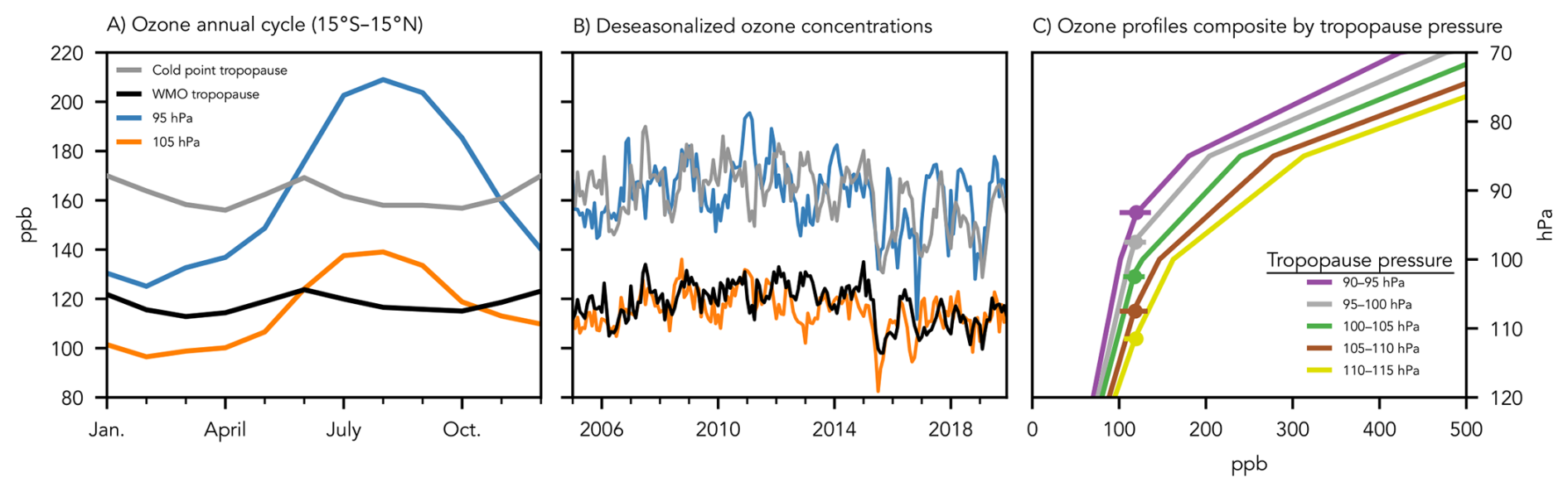
Figure 1 Ozone mixing ratios at and near the tropical tropopause, 2005–2019. (a) The annual cycle at the cold point tropopause (gray), WMO tropopause (black), 95 hPa (blue), and 105 hPa (orange). (b) Monthly time series at each level with the annual cycle removed. (c) Mean profiles in the tropical upper troposphere and lower stratosphere composited by tropopause pressure, with error bars spanning the 5th to 95th percentiles. Data are from MERRA2 and are averaged over 15° S to 15° N.

3 Results

3.1 Annual and interannual variability in observed tropical tropopause ozone

The annual cycles of ozone mixing ratios at the tropical tropopause and at two nearby fixed pressure levels (105 and 95 hPa) from 2005 to 2019 are shown in Fig. 1a. (See Fig. S2 for ozone and tropopause pressure annual cycles from SWOOSH and EUMETSAT ROM SAF products (Davis et al., 2016; Lauritsen et al., 2022).) Following from the strength of the stratospheric circulation, the flux of ozone-poor air into the stratosphere is strongest (weakest) in boreal winter (summer) (Rosenlof, 1995). Thus, ozone mixing ratios at 105 and 95 hPa reach their minima and maxima in January and August, respectively, in agreement with past work (Randel et al., 2007).

The annual cycle of ozone mixing ratios at the tropical tropopause is substantially smaller than the annual cycle at either 95 or 105 hPa, and it does not align with the annual cycle of upwelling. The relative amplitudes (peak-to-peak divided by the mean) of tropical ozone mixing ratios at the cold point tropopause and 95 hPa are 0.09 and 0.52, respectively, and tropopause ozone mixing ratios peak in January and June. A relative amplitude of 0.09 is also observed at the WMO tropopause, which is smaller than that shown on the 380 K isentrope (about 0.3) in Konopka et al. (2009). The annual cycle of ozone mixing ratios at the tropopause is therefore distinct from nearby fixed pressure or isentropic levels, implying that the effects of upwelling's annual cycle must be counterbalanced when following the tropopause pressure.

Interannual variability in ozone mixing ratios is similar in magnitude at the tropical tropopause and fixed pressure levels (Fig. 1b). However, variability at fixed pressures does not fully explain that at the tropopause – the Pearson correlation coefficient between deseasonalized ozone at the WMO (cold point) tropopause and at 105 (95) hPa is 0.31 (0.24). Two underlying modes of climate variability, the El Niño-Southern Oscillation (ENSO) and Quasi-Bienniel Oscillation (QBO), are also more strongly correlated with interannual ozone variability at fixed pressure levels (Fig. 2). In addition, the correlation between tropopause ozone and the QBO index is improved when lagged by 6 months (r=0.36 and 0.43 for WMO and cold point tropopauses, respectively; not shown), while the correlations between 95 and 105 hPa ozone and the QBO are maximized with no lag. Furthermore, multiple linear regression models of ozone variability with ENSO and QBO indices as predictors exhibit higher coefficients of determination at 95 and 105 hPa (r²=0.21, 0.17) than at the tropopause (r²=0.003 at both the cold point and WMO tropopause). Note that these coefficients account for temporal autocorrelation (AR(1)) in the ozone time series and are therefore lower than the square of the correlation coefficients shown in Fig. 2. Lastly, the deseasonalized WMO tropopause pressure correlates with deseasonalized ozone at 105 hPa with a coefficient of r=0.64 (r=0.72 between the cold point tropopause pressure and 95 hPa ozone), reflecting the influence of upwelling strength, but the tropopause pressure shows a weak negative correlation with ozone at the tropopause itself ($r=-\mathrm{0.06}$ and −0.20 for WMO and cold point tropopauses). These results indicate that different mechanisms may drive ozone variability at the tropical tropopause and at nearby fixed pressure levels.

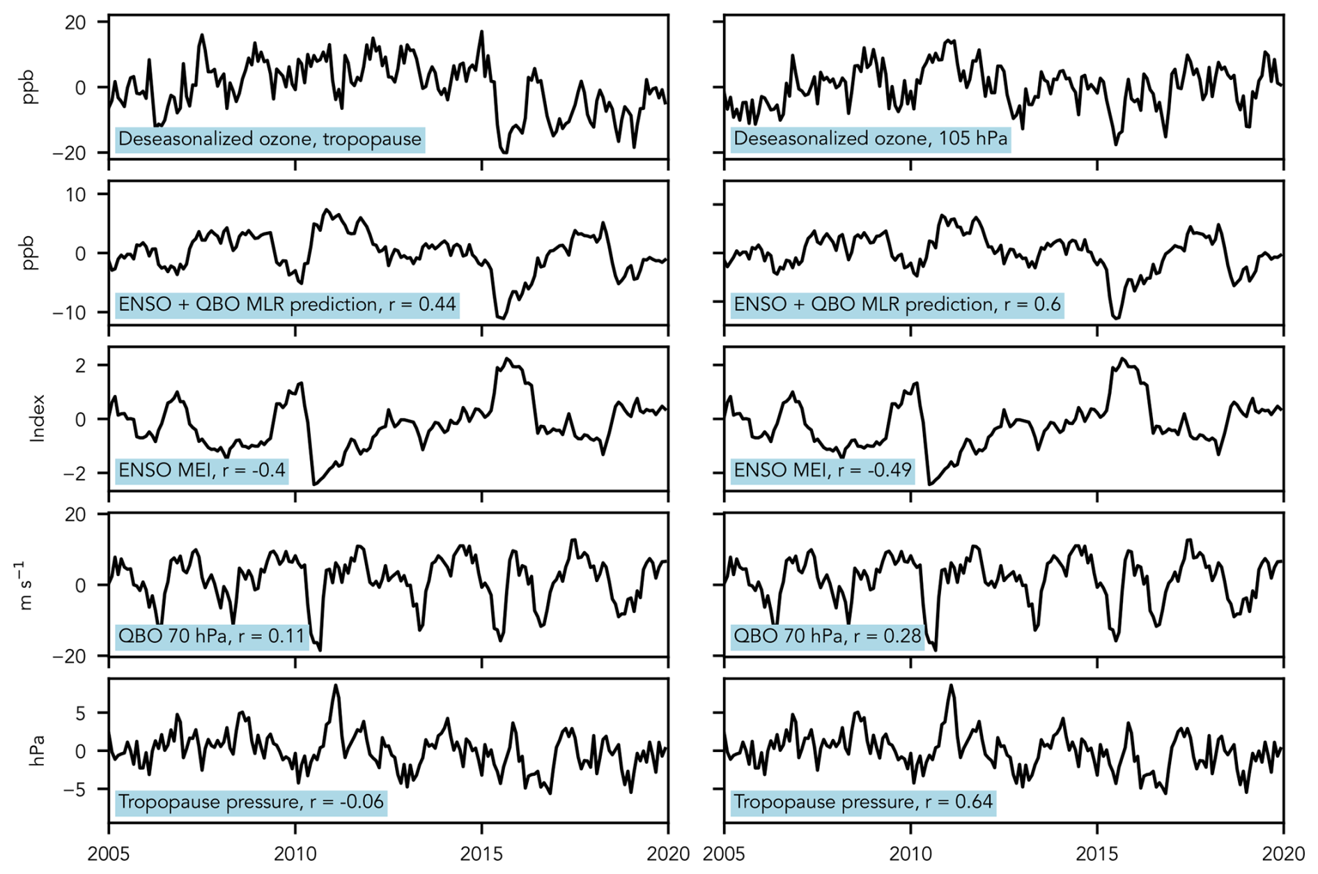
Figure 2 Deseasonalized ozone and correlations with expected drivers of interannual climate variability, 2005–2019. (Top row) Time series of deseasonalized ozone mixing ratios at the WMO tropopause (left) and 105 hPa (right), (second row) ozone mixing ratios as predicted by a multiple linear regression fit with ENSO and QBO indices, (third row) Multivariate ENSO Index Version 2 values, (fourth row) monthly zonal mean winds at 70 hPa measured over Singapore, and (bottom row) deseasonalized WMO tropopause pressure. Panels in the bottom four rows list correlations between each time series and the deseasonalized ozone mixing ratios shown in the column’s top panel. ENSO MEI values and 70 hPa winds were obtained from https://psl.noaa.gov/enso/mei/data/meiv2.data and https://www.geo.fu-berlin.de/en/met/ag/strat/produkte/qbo/, respectively (both last accessed: 7 November 2025).

To view the relationship between tropical tropopause pressure and near-tropopause ozone levels across all modes of variability from 2005 to 2019, we composite ozone profiles based on the monthly WMO tropopause pressure (Fig. 1c). This emphasizes the covariance between tropopause height and ozone mixing ratios at fixed pressure levels – as well as the invariance of tropical tropopause ozone mixing ratios. Mean ozone mixing ratios at the WMO tropopause (marked with circles) vary by 2 ppb as the tropopause pressure varies by 20 hPa, while ozone mixing ratios at 100 hPa covary with the movement of the tropopause, ranging from 102 to 162 ppb.

3.2 A budget for tropical tropopause ozone

As shown in the previous section, ozone mixing ratios at the tropical tropopause and at nearby fixed pressure levels have distinct modes of variability, motivating inspection of the underlying ozone budgets. Here, we carry out this analysis using our budget equations (Eqs. 1 and 2) at the time-mean tropical tropopause pressure (102 hPa) and at time-varying tropopause pressures, and we compare our budget-derived tendencies with observed changes in ozone mixing ratios. See Fig. S1 for a validation of this method with output the Community Earth System Model version 1 run with the Whole Atmosphere Chemistry Climate Model (Marsh et al., 2013).

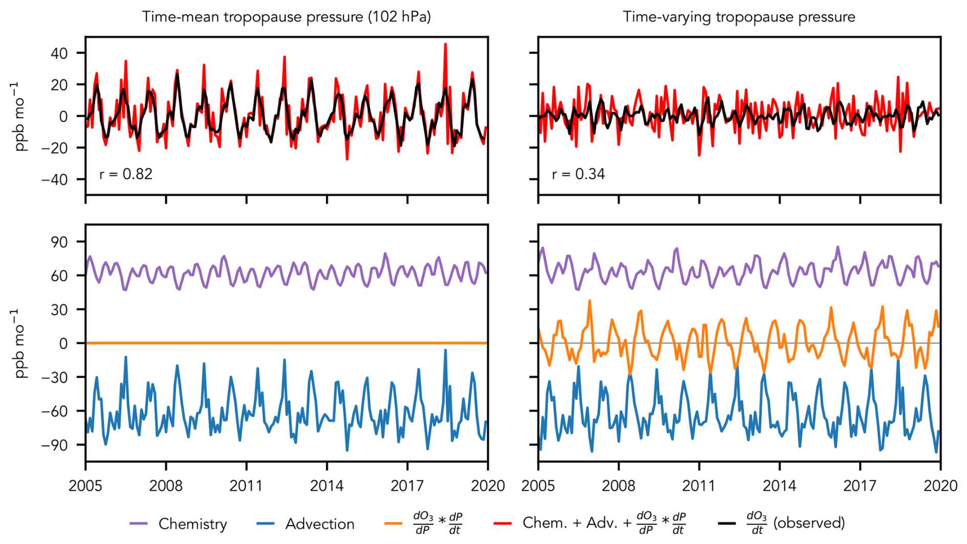
Figure 3 Ozone budget equations evaluated at the time-mean tropical tropopause pressure (left column) and at the time-resolved tropical tropopause (right column) from 2005 to 2019. Chemistry (purple) and advection (blue) budget terms are from MERRA2-GMI, and the tendency from the monthly change in tropopause pressure (orange) is computed from MERRA2 ozone profiles and tropopause pressures from Hoffmann and Spang (2021). Observed changes to ozone mixing ratios are included (black lines), along with the correlation coefficients between the budget-based tendency (red) and observations.

The ozone tendency at 102 hPa is recovered well by our assumed ozone budget for fixed pressure levels (Eq. 1), with a correlation of r=0.82 between the two and a coherent annual cycle (Fig. 3, left panel). Note that greater monthly variability is expected for the budget reconstruction, as the observed change in tropopause ozone is calculated using central differences; the correlation improves to r=0.94 when the budget tendency is smoothed using a three-month running mean (Fig. A1). This agreement gives confidence to our chemistry-advection budget within the context of MERRA2-GMI ozone profiles and tendencies. Meanwhile, the budget-derived ozone tendency at the time-varying tropopause shows lower amplitude variability than the budget at 102 hPa and is moderately correlated with observations (r=0.34). Importantly, the agreement between the budget-derived tendency and observations is improved by including the change-in-height term, with no correlation (r<0.01, not shown) when the term is removed (i.e., when Eq. 1 is used instead of Eq. 2). Although chemical production and advection are the dominant terms by magnitude in both analyses, Fig. 3 confirms that the ozone budget at the time-varying tropical tropopause is distinct from the budget at a nearby fixed pressure level.

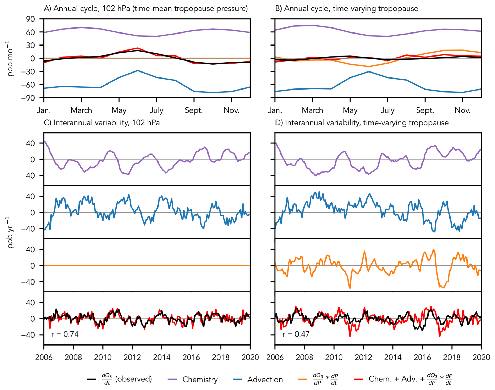
Figure 4 The budget for ozone mixing ratios near the tropopause on monthly and interannual timescales. The annual cycle of the ozone budget evaluated at (a) the time-mean tropopause pressure and (b) the time-varying tropopause, and (c, d) the interannual budget for the time-mean and time-varying tropopause pressures with each tendency term plotted separately. The tendencies in c and d are summed over the preceding 12 months, and the observed annual change in ozone is calculated for each month as the difference from 12 months prior (see Eqs. 6 and 7). Chemistry (purple) and advection (blue) budget terms are from MERRA2 GMI, and the tendency from the monthly change in pressure of the tropopause (orange) is computed from MERRA2 ozone profiles and tropopause pressures from Hoffmann and Spang (2021). Observed changes to ozone mixing ratios are included (black lines), along with the correlation coefficients between the budget-based tendency (red) and observations in panels (c) and (d).

To explore the differing modes of annual and interannual variability at the tropopause and at nearby fixed pressure levels, we separate ozone tendencies into annual cycle and deseasonalized time series. Figure 4a, b shows the annual cycle of ozone tendencies at the tropopause's time-mean pressure height (left panel) and at the time-varying tropical tropopause (right panel). For both budgets, the annual cycle of the advective tendency has a greater amplitude than the annual cycle of chemistry. This is consistent with the previously identified mechanism for upwelling-driven ozone variability near the tropical tropopause (Randel et al., 2007), as well as an increase in horizontal transport from the mid-latitudes during boreal summer (Abalos et al., 2013). At 102 hPa, the balance of these terms agrees well with the observed change in ozone mixing ratios, confirming that the two-term budget (Eq. 1) captures the annual cycle of net ozone tendencies at fixed pressure levels. The sum of the preceding year's chemical and advective tendencies is also strongly correlated with year-over-year change in ozone at 102 hPa (r=0.74; Fig. 4c). However, at the time-varying tropical tropopause, the balance of the chemical and advective tendencies results in too large of an annual cycle and interannual variability that is weakly correlated with observed changes (r=0.11, not shown).

The inclusion of a change-in-height term improves the fit between the budget-derived tendency and observed changes to tropical tropopause ozone for both the annual cycle and interannual variability (Fig. 4b, d). As the change in tropical tropopause pressure on annual-to-interannual timescales can be driven by variability in upwelling strength (Yulaeva et al., 1994; Boehm and Lee, 2003; Sweeney and Fu, 2024), while the vertical advection of ozone is negative, the change-in-height term computed here is anticorrelated with the advective ozone tendency. Thus, the annual cycle of the advective tendency is opposed by the movement of the tropopause along the background ozone gradient, and tropical tropopause ozone variability is suppressed. This change-in-height term also improves the match with observed interannual ozone anomalies relative to a chemistry-advection budget (r=0.47), although deviations between the two time series exist (e.g., the negative anomaly in observations around 2016).

Increased photochemical ozone production at the time-varying tropopause during extended boreal winter also contributes to the dampened annual cycle, although as a secondary mechanism. In the tropics, photochemical ozone production has a biannual cycle, with maxima at the equinoxes driven by cycling of incoming sunlight's incident angle (purple lines in Fig. 4a, b) (Perliski et al., 1989). In addition, incoming ultraviolet radiation near the tropopause is greater at the vernal equinox than the autumnal equinox due to an upwelling-driven reduction in overhead ozone during the preceding months (i.e., self-healing; Solomon et al., 1985), resulting in greater ozone production in boreal spring. Ozone production at the tropopause – but not at 102 hPa – is further modulated by changes in the tropopause pressure. The elevation of the tropopause in boreal winter moves the tropopause up the ozone production gradient, increasing the ozone chemical tendency at the tropopause in January by 12 % relative to 102 hPa.

3.3 Tropical tropopause ozone in a warming climate

While annual-to-interannual variability in the tropical tropopause pressure is partly driven by variations in upwelling strength, long-term changes may be driven by tropospheric expansion, which can increase the height of the tropopause independent of upwelling. Tropospheric expansion is a robust thermodynamic response of the atmosphere to surface warming, and while an accelerated stratospheric circulation is a concurrent response present in models (Abalos et al., 2021; Rind et al., 1990; Butchart et al., 2006; Hardiman et al., 2014) it has not been unambiguously detected in observations (Mahieu et al., 2014; Harrison et al., 2016; Schoeberl et al., 2008; Engel et al., 2009; Fu et al., 2019; Bourguet et al., 2025). All else equal, these two drivers would have competing impacts on the tropical tropopause ozone budget: Tropospheric expansion shifts the tropopause into a region of increased ozone production, while enhanced upwelling increases advection of ozone-poor air from the troposphere.

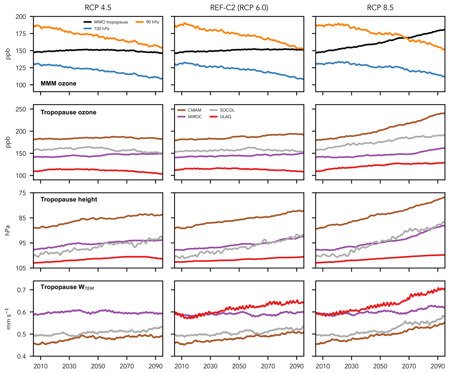
Figure 5 CCMI projections of tropical tropopause ozone mixing ratios, pressures, and upwelling velocities under three warming scenarios. (Top row) Multi-model mean ozone mixing ratios at the tropical WMO tropopause (black) and two nearby fixed pressure levels (90 and 100 hPa; blue and orange, respectively), (second row) tropical tropopause ozone mixing ratios for CMAM (green), SOCOL (purple), MIROC (red), and ULAQ (brown), (third row) WMO tropopause pressures, and (bottom row) transformed Eulerian mean vertical velocities. All time series are 120-month running mean, zonal mean, and tropical (15° S–15° N) mean.

In the context of these competing mechanisms, we explore how tropical tropopause ozone evolves with surface warming in four models submitted to CCMI run with senC2RCP45, refC2, and senC2RCP85 specifications (RCP4.5, RCP6.0, and RCP8.5 greenhouse forcing, respectively; hereafter referred to by their RCP forcings). These models each show a suppressed annual cycle of ozone mixing ratios at the tropical tropopause, similar to observations (Fig. S3), suggesting a level of accuracy in their tropopause ozone budgets. Following from the expected impacts of enhanced upwelling and tropospheric expansion (Match and Gerber, 2022), multi-model mean ozone mixing ratios at fixed pressure levels near the tropopause (90 and 100 hPa) decrease by the end of the century in each of the forcing scenarios (Fig. 5, top row). Meanwhile, multi-model mean tropical tropopause ozone mixing ratios decrease by less than 1 % from 2000–2010 to 2090–2099 under RCP4.5 forcing and increase by 3 % and 23 % under RCP6.0 and RCP8.5 forcing, respectively. Thus, variability in ozone mixing ratios at the tropopause remains distinct from variability at fixed pressure levels when driven by long-term surface warming.

As changes to tropopause pressure and upwelling have competing effects on the tropical tropopause ozone budget, we examine their trends in the four CCMI simulations in the bottom two rows of Fig. 5. Tropopause pressure decreases and upwelling increases in all simulations, although the increase in upwelling is not significant under RCP4.5 or RCP6.0 forcing in MIROC. In all simulations, increases to upwelling at the tropopause are dampened relative to fixed pressure levels (Fig. A2), consistent with previous work on lower stratospheric upwelling in tropopause-relative coordinates (Oberländer-Hayn et al., 2016). Notably, the model with the lowest tropopause pressure and weakest upwelling (CMAM) also has the highest tropopause ozone mixing ratio and greatest increase in ozone under RCP8.5 forcing. Conversely, the model with the highest tropopause pressure and greatest increase in upwelling (ULAQ) has the lowest tropical tropopause ozone and exhibits a decrease in the two weaker forcing scenarios. The trends in these end-members can be understood according to our ozone budget framework. Ozone production is enhanced more rapidly in CMAM due to faster tropospheric expansion and a sharper ozone production gradient (due to a higher initial tropopause), while a weaker increase in ozone production is countered by a stronger negative advective tendency in ULAQ.

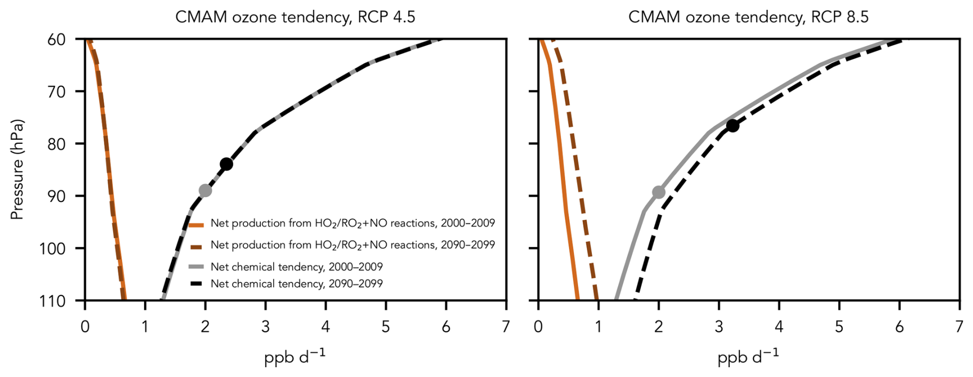
Figure 6 Changes to CMAM ozone production rates in two warming scenarios. Decadal averages of net ozone production from HO_x and NO_x reactions (tan and brown) and net chemical tendencies (gray and black) in 2000–2009 and 2090–2099 for RCP4.5 (left) and RCP8.5 (right) projections. Rates between grid points are interpolated in log-pressure coordinates, and the tropical tropopause pressure for each time period is marked by dots. Note the increase in ozone production at the tropopause in both scenarios due to changes in tropopause pressure, as well as the underlying increase in ozone production throughout the region from HO_x and NO_x reactions in RCP8.5.

We further investigate changes to tropical tropopause ozone in CMAM by examining the model's ozone production rates under RCP4.5 and RCP8.5 forcing. Net chemical ozone tendencies and production and loss rates due to HO_x and NO_x reactions are provided from this model, allowing production changes due to oxygen photolysis rates and precursor chemistry to be disentangled. We find that ozone production increases at the tropopause in both forcing scenarios due to tropospheric expansion (Fig. 6), supporting the above budget analysis. We isolate this expansion-driven increase by evaluating 2000–2009 production rates at the 2000–2009 and 2090–2099 tropical tropopause pressures and find increases of 0.35 and 0.92 ppb d⁻¹ (17 % and 46 %) in RCP4.5 and RCP8.5, respectively, between the time periods. Ozone production rates due to HO_x and NO_x chemistry also increase at fixed pressure levels in the upper troposphere and lower stratosphere under RCP8.5 forcing. Increased anthropogenic emissions specified in the RCP8.5 scenario lead to changes in tropospheric composition, including increased methane abundances (Eyring et al., 2013a), that strengthen these production rates at 89 hPa (the 2000–2009 tropical tropopause pressure in CMAM) by 0.26 ppb d⁻¹, or 62 %, by the end of the century. Although this contributes to increased tropical tropopause ozone in RCP8.5, the primary driver of increased ozone production at the tropical tropopause is tropospheric expansion in this simulation, and it is the sole driver in RCP4.5.

We note that changes to in-mixing of ozone-rich mid-latitude air are not considered here, as previous modeling work has shown that warming-driven changes to eddy mixing are eliminated when using tropopause-relative coordinates (Abalos et al., 2017). However, in-mixing of ozone may still increase as ozone mixing ratios in the mid-latitude lower stratosphere are elevated by the recovery of the ozone layer and an acceleration of the stratospheric circulation (Shepherd, 2008; Match and Gerber, 2022). Thus, increased ozone production at the tropical tropopause may be one of several contributing drivers that underlie projected ozone mixing ratio trends at the tropical tropopause.

4 Discussion

4.1 Implications for tropopause warming

Ozone is a key radiative species near the tropopause (Birner and Charlesworth, 2017; Charlesworth et al., 2019). Trends in tropopause ozone mixing ratios, such as those shown in Fig. 5, impact local temperatures, which in turn have a first-order control on the water vapor content of air entering the stratosphere and the static stability gradient between the upper troposphere and lower stratosphere. Although changes to tropopause temperatures can be driven by additional interacting factors, including local upwelling and water vapor concentrations, we briefly explore the relationship between tropical tropopause ozone and temperatures across 22 CCMI simulations in Fig. 7. Simulations were chosen based on the availability of necessary outputs (tropopause pressure and temperature, and zonal mean air temperature and ozone; see Fig. 7 legend for list of models) and include four RCP forcing scenarios (2.6, 4.5, 6.0, and 8.5). Therefore, this comparison captures a range of radiative and chemical forcings and responses. Changes are computed from the last decade of simulation (either 2090–2099 or 2091–2100) relative to 2000–2009, and changes to tropical tropopause temperatures are normalized by the increase in surface temperatures to account for warming driven by nonlocal radiative effects. This metric can be thought of as a tropopause response to surface warming, which is influenced by local ozone mixing ratios.

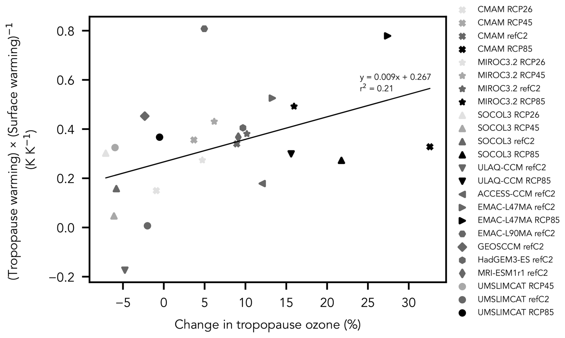
Figure 7 Scatter plot of the change in tropical tropopause temperature normalized by surface warming versus the fractional change in tropical tropopause ozone for CCMI simulations. Model names and simulation specifications are listed in the legend. Changes are computed for the final decade of the simulation (either 2090–2099 or 2091–2100) relative to 2000–2009. A linear regression line with a coefficient of determination of r²=0.21 is included; the positive relationship suggests that ozone mixing ratios at the tropical tropopause contribute to local temperature changes.

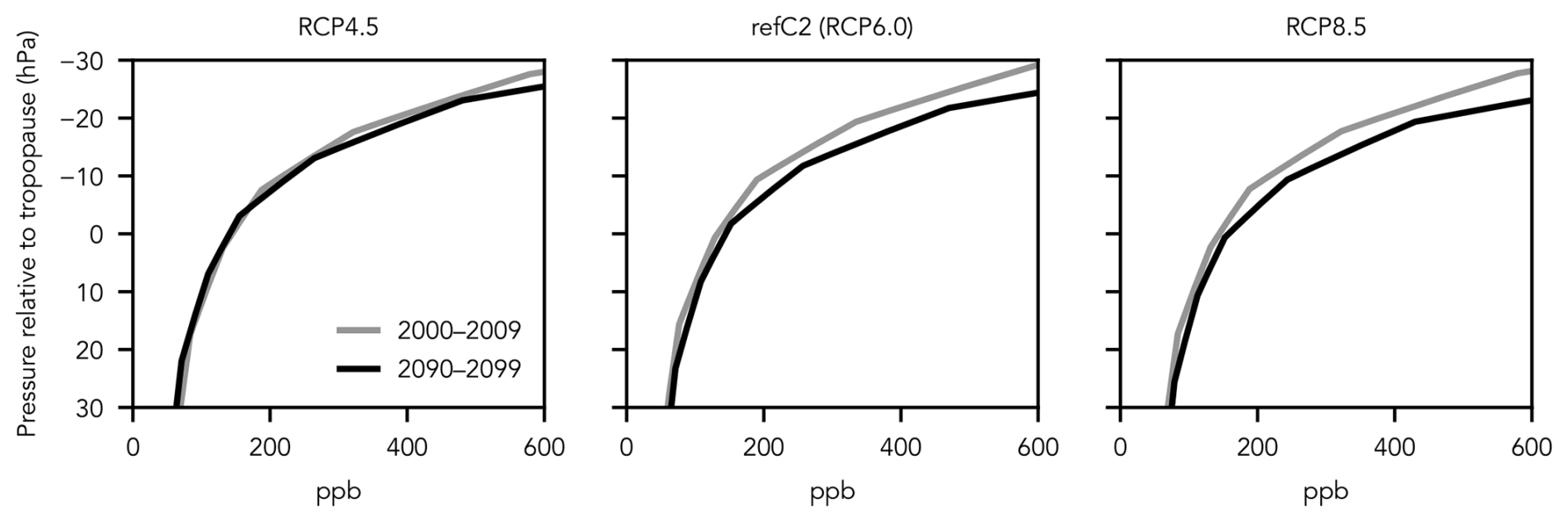
Figure 8 Multi-model mean tropical ozone mixing ratios at pressures relative to the tropical tropopause for four CCMI models under RCP4.5 (left), RCP6.0 (middle), and RCP8.5 (right) forcing. Gray lines are time-mean profiles for model years 2000–2009, and black lines are for model years 2090–2099.

As seen in Fig. 7, there is a weak positive relationship (r²=0.21) between changes to tropical tropopause ozone concentrations and temperatures. Although this relationship may exist in part due to the confounding influence of upwelling on both tropical tropopause ozone and temperature, ozone acts as an amplifying feedback to upwelling-driven changes to temperature (Charlesworth et al., 2019). Thus, the production-driven increase in tropical tropopause ozone presented here contributes to tropical tropopause warming.

It is also notable that tropical tropopause ozone increases with increased forcing for each model, with all models projecting an increase by the end of the century under RCP8.5 forcing. Assuming that ozone production rates exhibit similar trends across models, this can be understood from our analysis of CMAM production rates. The impact of tropospheric expansion on ozone production, and thereby ozone mixing ratios, is nonlinear due to the nonlinear relationship between ozone production and pressure (see Fig. 6). Thus, the additional warming and expansion driven by RCP8.5 forcing will have a greater per-hPa impact on tropical tropopause ozone than the weaker forcing scenarios. In other words, tropical tropopause ozone mixing ratios may not be meaningfully impacted by increased production following weak surface warming, but tropical tropopause ozone may ultimately increase as warming intensifies. A further increase may be driven by HO_x and NO_x chemistry depending on emissions. As changes to tropical tropopause ozone induce changes to local temperatures, this would lead to stratospheric moistening and initiate the stratospheric water vapor feedback (Dessler et al., 2013).

4.2 Implications for lower stratospheric ozone

Tropospheric expansion has previously been identified as a driver of lower stratospheric ozone reductions (Match and Gerber, 2022). Yet, here we have identified tropospheric expansion as a driver of increased tropical tropopause ozone – and therefore an increase in the ozone mixing ratios entering the stratosphere. These mechanisms appear at odds with each other; we reconcile this below.

Tropospheric expansion brings ozone-poor tropospheric air closer to fixed pressure levels in the lower stratosphere, which decreases the mass of ozone ascending from below (Match and Gerber, 2022). This contributes to the negative trend in ozone mixing ratios in CCMI simulations at 90 and 100 hPa seen in Fig. 5. However, the tropopause’s upward shift leads ascending tropospheric air to pass through a layer with enhanced photochemical ozone production. As a result, the rising tropospheric air accumulates more ozone by the time it reaches the tropopause, driving an increase in upper tropospheric ozone and allowing tropical tropopause ozone to increase in spite of the expansion of the troposphere's rapid ozone destruction regime. This effect would be dampened or possibly negated by enhanced upwelling; however, the apparent acceleration of the stratospheric circulation is substantially weaker when following the tropopause (Fig. A2; Oberländer-Hayn et al., 2016). Air that then ascends into the stratosphere from a heightened tropopause is exposed to greater ozone production due to the enhancement in photochemistry with height. Thus, following tropospheric expansion, tropical lower stratospheric ozone may increase due to (1) an increase in the ozone mixing ratio of air crossing the tropical tropopause, and (2) increased local ozone production rates. This mechanism should be stronger with greater surface warming and tropospheric expansion.

As seen in Fig. 8, CCMI simulations support our proposed mechanism: Lower stratospheric ozone increases by the end of the century under greenhouse forcing in tropopause-relative coordinates, with more substantial increases seen with greater forcing. This analysis is done for the volume mixing ratio (or mole fraction) of ozone, as this unit is not transformed by changes to tropopause pressure. Notably, Match and Gerber (2022) computed the ozone number density (a natural unit for understanding column ozone and its total radiative absorption), which is proportional to pressure in addition to mixing ratios – thus resulting in decreases at the tropopause and in the lower stratosphere following tropospheric expansion. More important, Match and Gerber (2022) presented results on fixed atmospheric heights; however, the ozone gradient above the tropopause would become sharper in their idealized photochemistry-transport model in a tropospheric-expansion-only scenario when the tropopause is followed upwards. Therefore, the mechanism here adds nuance to previous work without a necessary contradiction: Tropospheric expansion decreases ozone at fixed levels near the historical tropopause, but its effect on ozone at, below, and above the tropical tropopause may be reversed when accounting for a changed frame of reference.

5 Conclusions

In this work, we have shown that ozone mixing ratios at the tropical tropopause do not covary with mixing ratios at nearby fixed pressure levels. This is seen on annual and interannual timescales in observations, and it holds in future simulations of chemistry-climate models under a range of forcing scenarios. We show that a simple budget composed of advective and chemical tendencies can explain the annual cycle and interannual variability of ozone mixing ratios at the time-mean pressure of the tropical tropopause (102 hPa), consistent with past work on lower stratospheric ozone (Perliski et al., 1989; Avallone and Prather, 1996). However, an additional tendency that results from the change in pressure of the tropopause is needed to explain ozone variability when ozone mixing ratios are evaluated at the time-varying tropopause pressure. This term counterbalances the tendency induced by the annual cycle of upwelling in the lower stratosphere, resulting in a much weaker annual cycle of ozone at the tropical tropopause than at nearby fixed pressure levels. A greater portion of interannual ozone variability is also explained by the budget when this tendency is considered. Thus, analyses of ozone mixing ratios completed on fixed pressure levels near the tropopause cannot characterize tropopause ozone variability.

In model simulations of the 21st century submitted to CCMI, we find that trends in tropical tropopause ozone are either dampened relative to the decreases at 100 and 90 hPa or reversed in sign to a positive trend. We show that the movement of the tropical tropopause up the background ozone production gradient drives this difference, with a secondary effect from changes to HO_x and NO_x chemistry. As the ozone production gradient increases nonlinearly with height, photochemical ozone production at the tropical tropopause will strengthen at an increasing rate with greater climate forcing and additional tropospheric expansion. Thus, tropical tropopause ozone trends can be expected to become more positive with greater surface warming. Future work may consider if tropopause-level trends apply to the entire tropical tropopause layer (e.g., Fueglistaler et al., 2009). Furthermore, it should be noted the total mass of the stratosphere is reduced by tropospheric expansion, so total column ozone can still decrease despite the increase in ozone mixing ratios presented here. Due to the positive relationship between tropical tropopause ozone and local temperature, this work motivates future modeling efforts to properly represent the dynamic and photochemical environment of the tropical tropopause.

Appendix A

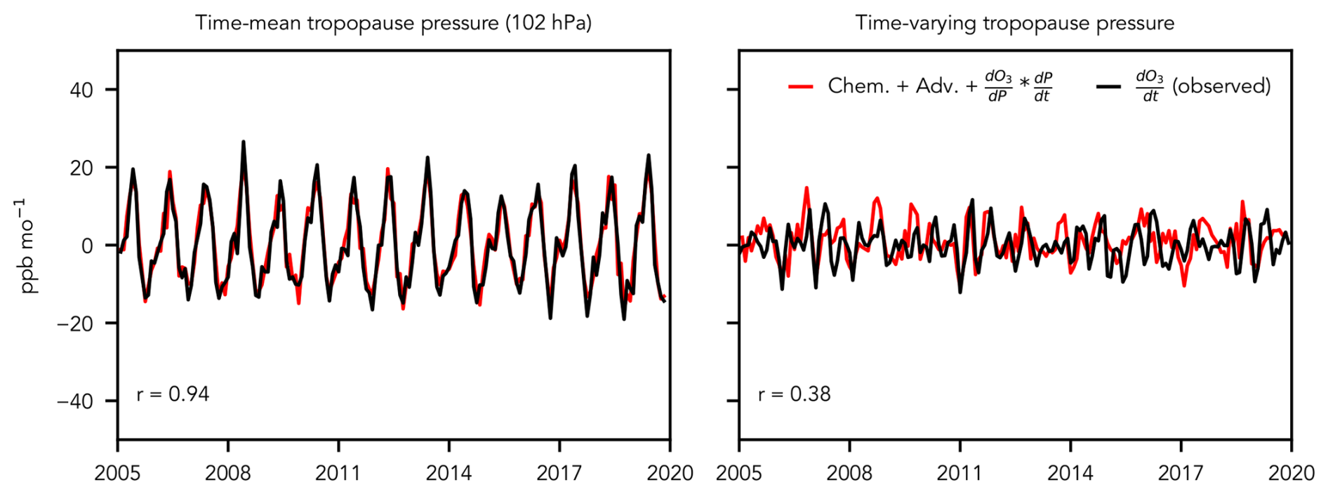
Figure A1 Same as top row of Main Text Fig. 3 but with the budget-derived tendency smoothed using a 3-month running mean.

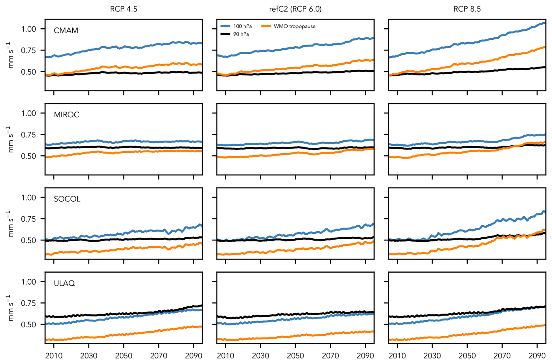
Figure A2 Transformed Eulerian mean vertical velocities at two pressure levels near the tropical tropopause (100 and 90 hPa; blue and orange, respectively) and at the tropical tropopause (black) under three forcing scenarios for four CCMI models. Note the difference between upwelling trends between the tropopause and fixed pressure levels. Also note the similarity between RCP4.5 and RCP8.5 simulations in ULAQ; given that the upwelling strength in both is greater than RCP6.0, we assume an error in the RCP4.5 upload.