Capturing and explaining the effects of three-dimensional radiative transfer on cloud evolution with the dynamic TenStream solver

Radiative transfer is an inherently three-dimensional (3D) process that, for computational reasons, is still approximated as one-dimensional (1D) in most atmospheric models. To address this limitation, Maier et al. (2024) introduced the dynamic TenStream solver, which reduces the cost of 3D radiative transfer calculations through incomplete solves. Here, we investigate how coupling dynamic TenStream to the large-eddy simulation model PALM affects cloud development compared to simulations using conventional 1D and full 3D radiation. Results show that during daytime, clouds driven by either of the 3D solvers organize into cloud streets oriented perpendicular to the solar incidence angle, whereas with 1D radiation they remain more or less randomly distributed. Moreover, daytime clouds grow larger, become thicker, and contain more liquid water with 3D radiative transfer. It is shown that these differences arise because, unlike in the 1D case, clouds coupled to 3D radiation are not positioned directly above their own shadows. Instead, they are located over areas of enhanced net surface irradiance, where values even exceed those in the clear-sky columns of the 1D simulation, strengthening rather than weakening the associated updrafts. Additionally, 3D radiation is shown to reduce the domain-averaged net thermal emission at the surface, which affects the surface energy budget and is primarily balanced by an increase in the domain-averaged latent heat flux, resulting in a greater release of water vapor into the atmosphere. Both effects are captured by dynamic TenStream, demonstrating its ability to represent 3D radiative effects on cloud development at a substantially lower computational cost.

1 Introduction

As numerical weather prediction (NWP) models move toward higher horizontal resolutions, inter-column three-dimensional (3D) radiative effects become increasingly important. At cloud-resolving scales, cloud shadows, for instance, are no longer confined to the vertical model columns of their respective clouds, but can extend into several neighboring ones. Additionally, radiation scattered from cloud sides can enhance the diffuse downward radiation in adjacent cloud-free columns (Hogan and Shonk, 2013), whereas radiation entering through gaps between clouds can become trapped between them and the surface, thereby increasing the diffuse downward radiation below clouds as well (Hogan et al., 2019). In the thermal spectral range, higher-resolution models feature more pronounced cloud-side cooling. Together, all of these 3D radiative effects influence the spatial distribution of sources and sinks of radiative energy in the atmosphere, which in turn drive the atmospheric circulation and the weather. Accurately capturing these effects is therefore crucial for predicting future atmospheric states.

However, the calculation of 3D radiative effects is computationally expensive, which has largely prevented their representation in operational forecasting. Instead, state-of-the-art NWP models still rely on one-dimensional (1D) independent column approximations, such as the Monte Carlo independent column approximation (McICA; Pincus et al., 2003) currently employed at both the Deutscher Wetterdienst (DWD) and the European Centre for Medium-Range Weather Forecasts (ECMWF) (DWD, 2021; Hogan and Bozzo, 2018). These models assume that radiative transport only takes place in the vertical and neglect any horizontal energy exchange. While this approximation generally performs well in horizontally homogeneous situations such as clear skies or completely overcast conditions, it breaks down as soon as numerous individual clouds shape the sky. Broken cloud fields, however, are common. Measurements conducted in Cabauw, the Netherlands, for instance, show that conditions that are neither clear sky nor overcast accounted for roughly half of the daylight time over a 10-year period, indicating that situations where 3D radiative effects can be important arise quite frequently (Mol et al., 2023). In such broken cloud fields, 3D radiative transfer has been shown to strongly influence both the organization and evolution of clouds. Klinger et al. (2017), for example, found that incorporating 3D radiative transfer in the thermal spectral range results in systematically larger cooling and stronger organizational effects compared to simulations performed with 1D radiative transfer approximations. Similarly, Jakub and Mayer (2017) demonstrated that inter-column 3D radiative transfer in the solar spectral range can foster the formation of cloud streets that are not observed to the same extent in 1D simulations. Furthermore, focusing on cloud characteristics, Veerman et al. (2020, 2022) and Tijhuis et al. (2024) showed that clouds in simulations coupled to 3D radiative transfer become thicker, grow larger in horizontal extent, and exhibit higher mean liquid water paths than their 1D-driven counterparts. Nonetheless, despite this demonstrated impact on cloud development, the implications of 3D radiative transfer on weather forecasts remain largely unexplored, primarily due to its high computational cost.

To address this issue, in recent years, considerable effort has been put into making 3D radiative transfer models computationally more feasible. Many such models simplify 3D radiative transfer calculations by considering only a discrete number of angles (e.g., Lovejoy et al., 1990; Gabriel et al., 1990; Davis et al., 1990). More recently, the TenStream solver (Jakub and Mayer, 2015) built upon this idea. It is capable of calculating 3D radiative fluxes and heating rates in both the solar and thermal spectral ranges by extending the 1D two-stream formulation to ten streams, thereby allowing for horizontal transport of energy. In contrast to these angular discretization methods, the neighboring column approximation (NCA; Klinger and Mayer, 2016, 2020) offers a fast analytical method for computing 3D heating rates in the thermal spectral range. To do so, it estimates cloud-side effects by taking only the immediate neighbors of a specific grid box into account. Apart from these two approaches, significant progress has also been made in accelerating highly accurate 3D Monte Carlo solvers for the use in large-eddy simulation (LES) models, with Veerman et al. (2022), for example, speeding up the method by utilizing graphics processing units (GPUs). This allowed them to perform LES runs driven by a full Monte Carlo solver for the first time ever.

Despite these advances, 3D solvers remain too slow to be used operationally. For instance, the GPU-accelerated Monte Carlo solver of Veerman et al. (2022) is still at least 6.4 times slower than the two-stream model it was compared to – and that only when using just 32 photons per spectral band and model column. At this low photon count, however, results remain notably noisy, both in irradiances and heating rates. Achieving substantially more accurate results, with root-mean-square errors of 6.88 W m⁻² in irradiances and 0.17 K d⁻¹ in heating rates, requires increasing the photon count eightfold to 256 photons per spectral band and model column, which raises the computational cost to 18.5 times that of the two-stream model. This high computational burden continues to prevent the use of 3D solvers in operational weather forecasting, especially given that radiation is already called far less frequently than the dynamical core in NWP models.

To overcome these limitations, Maier et al. (2024) took first steps toward a new “dynamic” 3D radiative transfer model: the dynamic TenStream solver. Currently designed for subkilometer-scale horizontal resolutions, where model grid boxes can be treated as homogeneous, it builds upon the original TenStream solver while introducing a novel approach that is speeding up inter-column radiative transfer by treating radiation more like model dynamics. Specifically, inspired by how NWP models integrate their primitive equations over time, the solver does not recalculate radiation from scratch each time it is called but instead updates the radiative field based on the result from the previous radiation time step. Starting from this updated field, it then performs only the first few steps of an iterative scheme toward the new solution, thereby limiting interactions to neighboring grid boxes. This approach not only enables a significant acceleration of radiative transfer calculations, but also facilitates the otherwise tedious parallelization of 3D radiative transfer methods, which typically require information from all parts of the domain. When coupled to a precalculated shallow cumulus cloud field, Maier et al. (2024) showed that this new solver is able to compute 3D heating rates and net surface irradiances at a noticeably faster speed than other 3D solvers, while also providing a significant improvement in terms of accuracy over currently employed 1D schemes.

Based on this work, the primary objective of this paper is to investigate how coupling the dynamic TenStream solver to model dynamics affects cloud development, and whether the new solver produces clouds that more closely resemble those driven by full 3D radiation than those coupled to a traditional 1D solver. In addition, this work aims to explore the mechanisms responsible for these differences. Because the current version of the dynamic TenStream solver assumes homogeneous grid boxes, we employed an LES model for this study. The setup of this model is described in Sect. 2 of this paper. Sect. 3 then discusses the differences between the simulations driven by 1D and 3D radiative transfer, whether the dynamic TenStream solver is able to capture them, and the mechanisms that may explain these differences. The paper concludes with a summary and outlook, given in Sect. 4.

2 Methodology

2.1 Simulation setup

All simulations discussed in this paper were performed with PALM (Raasch and Schröter, 2001; Maronga et al., 2015, 2020). Similar to the pre-calculated cloud fields used in Maier et al. (2024), the aim was to perform simulations in which shallow cumulus clouds develop over the course of the day. The purpose of this subsection is to provide an overview of how PALM was set up in order to generate these shallow cumulus cloud fields, as well as which simulations were ultimately performed.

2.1.1 Domain size

All simulations were performed with the same 100 m horizontal grid spacing that was used in Maier et al. (2024), but with 256×256 grid boxes, resulting in a 25.6×25.6 km² large domain – that is sixteen times the size used in the aforementioned study, allowing for improved statistics when assessing cloud characteristics dependent on the radiative transfer model used. In the vertical, 80 grid boxes with a spacing of 50 m were used, resulting in a domain that extends up to 4 km height. This comparatively low vertical resolution was chosen in order to reduce the storage demand of the simulation results while still ensuring a z–x aspect ratio below 1, just like in a typical NWP model.

2.1.2 Model initialization

The simulations, which represent an idealized case study, were set up for the geographic location of Munich, Germany (48.1° N, 11.6° E), but with its altitude set to 0 m, i.e., to sea level with a surface pressure of 1013.25 hPa. They were initially started on 14 June 2023 at 22:00 UTC, which corresponds to exactly midnight local time (00:00 CEST on 15 June 2023).

In addition to location and time, PALM required initial vertical profiles for potential temperature, total water mixing ratio, and zonal and meridional wind speed, which are shown in Fig. 1. They were chosen to suppress cloud formation prior to sunrise while allowing shallow cumulus clouds to develop and reach a limited vertical extent after surface heating begins. A purely westerly wind profile was prescribed, and the Coriolis force was disabled to maintain a stationary mean flow.

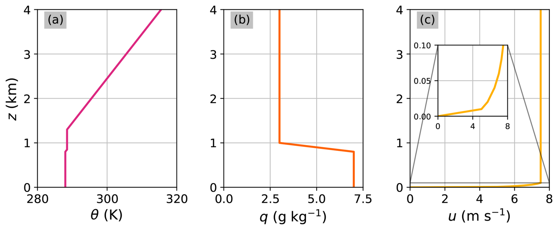
Figure 1 Initial profiles of the PALM simulations for potential temperature (a), total water mixing ratio (b), and zonal wind speed (c). The smaller graph in panel (c) shows a zoomed-in detail of the zonal wind speed profile between the surface and 100 m height.

The land–surface model of PALM was initialized with a flat, short grassland surface. Other than that, its setup was largely based on an example in the PALM documentation (PALM, 2026a), with only the soil temperature profile being modified to match the rest of the model initialization. Specifically, the soil temperature at the surface was set to 288 K, consistent with the potential temperature, and gradually decreased with depth to 280 K in the deepest soil layer. Additionally, the soil moisture was set to 0.18 m³ m⁻³ in all layers, which is somewhere between the wilting point (0.13 m³ m⁻³) and the saturation moisture (0.43 m³ m⁻³) of the medium-fine soil type used (PALM, 2026b).

For further details and to ensure that the simulations performed in this paper can be easily reproduced, you may refer to the parameter files used for the model runs, which are provided in Maier et al. (2026a) and Maier et al. (2026b).

2.1.3 Radiative transfer solvers

The main goal in terms of the setup was to perform different PALM simulations that vary only in the radiative transfer model used. To achieve this, we made use of the fact that the TenStream framework had been coupled to PALM in the past. Similar to the libRadtran library employed in Maier et al. (2024), this framework allows for the application of different radiative transfer solvers using an otherwise identical environment, and all the main features of the dynamic TenStream solver presented in Maier et al. (2024) have been implemented into it. In addition to that, the TenStream framework is fully parallelized. Hence, using this framework, and similar to the evaluation in Maier et al. (2024), the following radiative transfer solvers were applied:

1. A 1D δ-Eddington approximation

   This 1D approximation represents the type of radiative transfer scheme used in most models today and serves as a worst-case benchmark for evaluating the dynamic TenStream solver.

2. The dynamic TenStream solver

   The dynamic TenStream solver introduced in Maier et al. (2024) is the main focus of this evaluation. It is a comparatively fast 3D radiative transfer solver that reduces the cost of 3D radiative transfer calculations through incomplete solves. In the offline benchmarks of Maier et al. (2024), it was shown to be about three times slower than a traditional 1D δ-Eddington approximation, but substantially faster than other currently available 3D solvers. For the simulations presented here, it was configured to perform a full TenStream solve on its first use. After that, it was operated with a minimum of just two Gauß–Seidel iterations for diffuse radiation and one for direct solar radiation each time it was called. Since this implementation of the dynamic TenStream solver is fully parallelized, the iterations are performed independently on each subdomain, with communication between the cores occurring only once at the end of each radiation scheme call. The motivation behind this setup mirrors that in Maier et al. (2024): by applying a full 3D solve in the beginning, one can assess whether subsequent incomplete solves lead to different results than simulations using full TenStream solves throughout. Furthermore, as explained in Maier et al. (2024), using two iterations instead of one ensures that the iteration direction through the underlying system of linear equations is altered at least once per call.

3. The original TenStream solver

   Simulations performed with the original TenStream solver, also referred to as TenStream reference solver from here on, serve as benchmark simulations. Since the dynamic TenStream solver is based on this original TenStream model, reproducing its results despite using incomplete solves represents the best possible outcome.

The exact tenstream.options files used for the simulations with each of these solvers can be found in Maier et al. (2026a) and Maier et al. (2026b). Regardless of the radiative transfer solver applied, the atmospheric trace gas concentrations were provided by the 1976 US standard atmosphere (Anderson et al., 1986). Furthermore, all PALM simulations were carried out with a radiation time step of 30 s, as this proved to be a good speed-accuracy trade-off for the radiative transfer calculations in Maier et al. (2024), which were performed with the same horizontal grid spacing of 100 m.

2.1.4 Overview of the PALM simulation setup

Using these radiative transfer solvers, we can now discuss the different PALM simulations that were performed with them. A schematic overview of the setup is provided in Fig. 2. It shows that initially, five different simulations were conducted: a main run and four statistically independent but otherwise identical control runs. All of these simulations were started on 14 June 2023 at 22:00 UTC using the model initialization described earlier. The only difference between the simulations is that, at certain times (every 150 s in our runs), different random seeds of perturbations were applied to their horizontal wind fields until a predefined perturbation kinetic energy limit was reached. This limit was set to the default value of 0.01 m² s⁻². The resulting slightly different wind fields in the runs represent the uncertainties in the initial conditions of the setup and effectively create a five-member ensemble, enabling an estimation of whether certain features in an individual run are robust or fall within the simulation's inherent uncertainty.

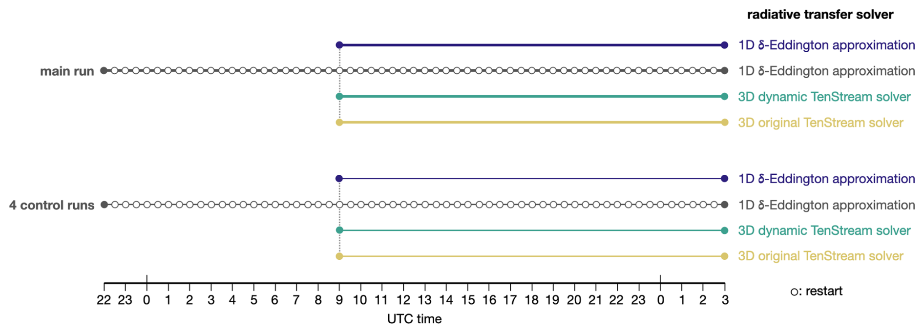
Figure 2 Schematic illustration of all PALM simulations discussed in this paper. On 14 June 2023 at 22:00 UTC, five simulations, a main run and four statistically independent but otherwise identical control runs (all shown in gray here), were started. These five initial model runs were driven by 1D radiation and restarted every 30 min, as indicated by the open circles in their respective timelines. Starting at 09:00 UTC on 15 June 2023, three additional restart runs were launched from each of these five initial runs. All these in total 15 restart runs were performed without further restarts and differed only in the radiative transfer model applied: the purple runs were driven by a 1D δ-Eddington approximation, the turquoise ones by the dynamic TenStream solver, and the ochre ones by the original TenStream solver, resulting in a five-member ensemble for each radiative transfer solver. Filled circles, in contrast to the open circles, visualize the start and end points of each PALM simulation.

From these slightly differently perturbed initial states, the simulations then ran for 29 h, ending on 16 June 2023 at 03:00 UTC. During this time, they were first given enough time to spin up and adjust their initial state until the Sun rose on 15 June 2023 at 03:13 UTC. After sunrise, the model runs then encompassed almost a full diurnal cycle, including sunset at 19:15 UTC and ending shortly before the next sunrise on 16 June 2023 at 03:12 UTC. Throughout this entire time, all five initial runs were driven by 1D radiation and restarted every 30 min. At each of these restart points, visualized by the open circles in Fig. 2, PALM stopped the simulation and saved its current state, before restarting it from exactly this saved atmospheric state.

Now, remember that our objective was to conduct different PALM simulations that vary only in the radiative transfer model used. The restart mechanism allows such simulations to be initiated from any intermediate time step shown in Fig. 2 by restarting the model run from the corresponding saved atmospheric state with modified runtime parameters, i.e., different radiative transfer solvers in this case. For this evaluation, the simulations were restarted from 09:00 UTC, i.e, 11:00 a.m. local time. At this point in time, shallow cumulus clouds have just started to form in the domain, making it a suitable moment for investigating how the subsequent development of these clouds and the surrounding atmosphere differs depending on the radiative transfer solver used. Consequently, starting from 09:00 UTC, three different restart runs were performed for every one of the five initial runs, each coupled to one of the three different radiative transfer solvers introduced above: either the 1D δ-Eddington approximation (shown in purple in Fig. 2), the dynamic TenStream solver (turquoise), or the original TenStream solver (ochre). These restart runs form the main foundation for the evaluation in this paper. Performing them for every ensemble member was important, as it will allow us to assess whether differences between runs driven by different radiative transfer solvers are robust compared to the ensemble spread. Apart from that, all restart runs were conducted without further restarts. They ran exactly as long as the five initial runs, i.e., until 16 June 2023 at 03:00 UTC, that is 05:00 a.m. local time, covering approximately ten hours of daytime and eight hours of nighttime, thereby providing a robust dataset for analyzing both of these regimes.

In terms of the general runtime configuration, all simulations were performed with a model time step of 5 s. Moreover, they were all executed on 64 CPU cores, using an 8 × 8 grid of subdomains, each containing 32 × 32 vertical columns. This domain decomposition is particularly important for the dynamic TenStream solver, since its incomplete solves are performed for each of the subdomains in parallel, with interaction between subdomains occurring only once at the end of each radiation scheme call. Information can thus only spread within individual subdomains during the radiative transfer calculations, and propagation to neighboring subdomains is delayed to subsequent calls of the scheme.

Regarding the cloud model, the built-in “morrison” scheme was applied, which uses two-moment cloud microphysics according to Seifert and Beheng (2005), Khairoutdinov and Kogan (2000), Khvorostyanov and Curry (2006) and Morrison and Grabowski (2007). Cloud water sedimentation was enabled, while aerosol concentration and cloud droplet number density were prescribed using the default values of PALM. Lastly, the data output for all the model runs was written at a temporal resolution of 60 s. This is considerably coarser than the 10 s resolution used in Maier et al. (2024), but a necessary reduction in terms of the overall storage size of the simulations. Although this means that output is only available for every second radiation time step, Sect. 3.2 will show that the averaged cloud characteristics primarily analyzed in this paper vary on much longer temporal scales, making this reduced output frequency also a scientifically acceptable compromise.

2.2 Evaluation methods

The entire evaluation in this paper is focused on the three five-member ensembles introduced above, i.e., the simulations shown in color in Fig. 2, which, started from either the main or one of the four control runs of the setup, are driven by the 1D δ-Eddington approximation, the dynamic TenStream solver, or the original TenStream solver. Using these simulations, our primary objective is to investigate whether, for each ensemble member, the atmosphere and its clouds develop differently depending on whether 1D or 3D radiation is applied. Additionally, and even more important for this work, our aim is to assess whether the dynamic TenStream solver is able to reproduce these potential 3D-related differences.

2.2.1 Accuracy evaluation

One way to investigate the aforementioned differences is by comparing the temporal evolution of selected model quantities across simulations driven by different radiative transfer solvers. Since the solvers fully interact with the model dynamics in these simulations, this evaluation is not just limited to radiative quantities but can also include other variables, such as the cloud water mixing ratio. For any such quantity ξ and at any point in time, the accuracy of a simulation relative to the corresponding TenStream reference run can be quantified using the mean bias error (MBE), which is given by

$$\begin{array}{}\text{(1)}& \mathrm{MBE}=\langle \mathit{\xi }\rangle -\langle {\mathit{\xi }}_{\text{ref}}\rangle =\langle \mathit{\xi }-{\mathit{\xi }}_{\text{ref}}\rangle ,\end{array}$$

where 〈…〉 denotes an arithmetic average over the considered model grid boxes. For each ensemble member, the MBE is calculated relative to the corresponding TenStream reference run initialized from the same restart state. The resulting five paired biases are then averaged to obtain the ensemble-mean bias, while their minimum-to-maximum range is used as an estimate of the ensemble spread.

Point-based error measures, such as the mean absolute error or root-mean-square error, however, are not utilized in this evaluation. This is because simulations coupled to different radiative transfer solvers lead to diverging atmospheric states, particularly in terms of clouds. Hence, even if two simulations featured clouds with nearly identical characteristics, slight positional differences could result in substantial errors when using point-based error metrics. Consequently, since this evaluation focuses on differences in cloud properties rather than on differences in the clouds' exact spatial placement, such error measures have not been applied. The MBE, by contrast, is based on averaged values and is therefore unaffected by these double-penalty errors.

At this point, it should also be noted that MBE values must be interpreted relative to the intrinsic variability of the simulations, which is estimated from the spread across the five paired ensemble members. A radiative transfer solver is therefore only considered to differ robustly from the TenStream reference solver if the MBE values of all five ensemble members, as indicated by the corresponding ensemble spread, clearly lie either above or below zero. Likewise, differences between simulations driven by different radiative transfer solvers are only regarded as meaningful if their ensemble ranges are clearly separated from each other.

2.2.2 Quantification of cloud characteristics

Apart from the temporal evolution of the MBE in certain model quantities, a particular interest lies in how the clouds in the simulations develop depending on the radiative transfer solver used. Therefore, inspired by the work of Tijhuis et al. (2024), three quantities are used to characterize the cloud fields at any point in time: cloud cover, average liquid water path (LWP) in cloudy columns, and average cloud depth. A grid box is defined as cloudy if its cloud water mixing ratio q_c exceeds 0.01 g kg⁻¹. The application of this threshold is necessary because many grid boxes in the simulations are subject to very small q_c values, often as low as 10⁻³⁵ g kg⁻¹. While physically negligible, the large number of these very small values strongly influences quantities such as cloud cover, so they are excluded from the analysis by applying the aforementioned threshold. The three cloud characteristic measures can then be defined as follows:

1. Cloud cover

   At any point in time, the cloud cover is given by the fraction of vertical columns in the domain that contain at least one grid box with q_c>0.01 g kg⁻¹.

2. Average liquid water path in cloudy columns

   This quantity is defined as the mean LWP of all vertical columns that contain at least one grid box with q_c>0.01 g kg⁻¹.

3. Average cloud depth

   For every cloudy column (i,j), the index of the highest ($k_{\max ,i,j}$) and lowest ($k_{\min ,i,j}$) grid box with q_c>0.01 g kg⁻¹ is determined. The cloud depth in this column is then given by

   $$\begin{array}{}\text{(2)}& \mathrm{\Delta }{z}_{\mathrm{cld},i,j}=\left(k_{\max ,i,j}+\mathrm{1}-k_{\min ,i,j}\right)\mathrm{\Delta }z,\end{array}$$

   where Δz is the vertical grid spacing. The average cloud depth is subsequently calculated as the mean of $\mathrm{\Delta }{z}_{\mathrm{cld},i,j}$ across all cloudy columns. Note that this method assumes only one cloudy layer per column, as cloud depths are calculated from the vertical extent between the highest and lowest cloudy model levels in each column, ignoring any cloud-free layers in between. This assumption, however, is valid for the shallow cumulus clouds used in this evaluation.

At this point, it is important to note that all these quantities describe general characteristics of cloud fields rather than properties of individual clouds. This is precisely the goal, as the objective of this paper is to identify systematic differences between cloud fields driven by 1D and 3D radiation. Moreover, unlike the work of Tijhuis et al. (2024), our evaluation also accounts for radiative transfer in the thermal spectral range, enabling the investigation of these differences during nighttime as well.

3 Discussion of the results

3.1 Simulation overview

Before getting into details, let us first take a look at the general evolution of the clouds in the different simulations. To this end, Fig. 3 shows five snapshots of the temporal evolution of the LWP in the simulations driven by the 1D δ-Eddington approximation, the dynamic TenStream solver, and the original TenStream model. For this overview, only simulations started from the main run of the setup are shown. Plots of the LWP are used because this quantity provides a good measure of both cloud position and thickness.

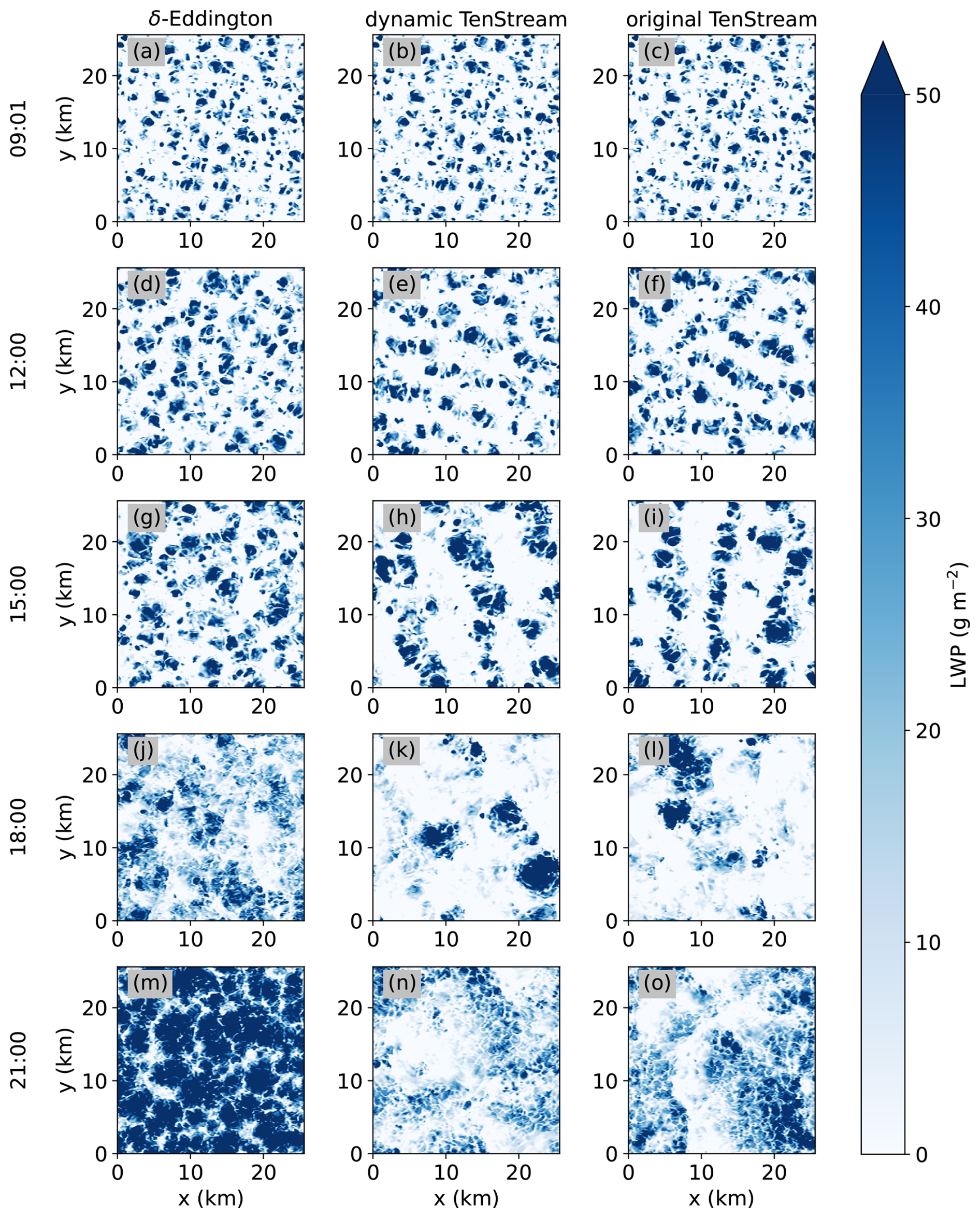
Figure 3 Temporal evolution of the liquid water path (LWP) in the PALM simulations driven by the 1D δ-Eddington approximation (left), the dynamic TenStream solver (middle), and the original TenStream model (right), shown for five time steps between 09:01 and 21:00 UTC. To enhance the contrast of the plots, the maximum LWP value for the colorbar was set to 50 g m⁻² instead of the global maximum value of 363 g m⁻².

Starting with the first row of panels, we can see that initially, all simulations of the main run were indeed started from the same cloud field, allowing differences in their subsequent development to be observed depending on the radiative transfer solver used. Results are shown for 09:01 UTC instead of 09:00 UTC for this first time step, as model output is not immediately available after the simulations start at 09:00 UTC. Three hours later, at 12:00 UTC, the clouds coupled to the different radiative transfer solvers have already developed differently. While they all increased in size compared to the plots at 09:01 UTC, we can clearly see that their organization differs between the simulation driven by 1D radiation shown in panel (d) and the one driven by the original TenStream model shown in panel (f). The clouds in panel (d) are still rather unorganized. In panel (f), however, we can observe the build-up of cloud streets, just as they were proposed in Jakub and Mayer (2017). These cloud streets are expected to form perpendicular to the angle of solar incidence and parallel to the mean wind flow. The latter is a constant westerly flow, whereas the Sun is positioned at an azimuth angle of 205° at 12:00 UTC, i.e., in the south–south–west. And indeed, the clouds are oriented perpendicular to that direction, forming streets with an east–south–easterly orientation, which is particularly visible in the lower right part of panel (f). The cloud streets are also visible in the simulation coupled to the dynamic TenStream solver shown in panel (e), providing a first example of a 3D-related effect that is captured by the dynamic treatment of radiation in that solver.

Moving on to panels (g)–(i), another three hours later, the cloud streets in the simulations coupled to 3D radiative transfer have become markedly more pronounced. Because the Sun moved to an azimuth angle of 262° in the meantime, which is almost exactly in the west, the cloud streets are oriented from north to south now, still perpendicular to the angle of solar incidence. In contrast to that, the clouds in the simulation driven by 1D radiation are still more or less randomly positioned. This absence of organization in the simulation driven by 1D radiation together with organization perpendicular to the mean westerly flow in the simulations coupled to 3D radiative transfer indicates that the cloud streets in these simulations are not dynamically induced, but really driven by radiation. Moreover, extending beyond the idealized setup of Jakub and Mayer (2017), this demonstrates, to our knowledge, for the first time that radiatively driven cloud streets can also form under a realistic diurnal cycle, with their orientation following the changing solar azimuth angle. Apart from these organizational aspects, we can also see that individual clouds in both panels (h) and (i) are noticeably larger in horizontal extent than those in panel (g). In fact, as we will discuss in Sect. 3.2, the clouds driven by the two 3D solvers grow larger in both horizontal and vertical extent during daytime. Their greater vertical extent, however, is not directly apparent from panels (h) and (i) because the LWP color scale in Fig. 3 saturates above 50 g m⁻² to enhance contrast. Apart from that, however, this development of larger and thicker clouds during daytime in simulations driven by 3D radiative transfer is consistent with findings in other studies (Veerman et al., 2020; Tijhuis et al., 2024).

As the day proceeds, the organization of clouds in the simulations driven by 3D radiative transfer starts to break down and is no longer visible in plots (k) and (l) at 18:00 UTC. However, this is also only about an hour before sunset at 19:15 UTC, with the Sun already at a relatively low elevation of 10°. It is also around this point in time that the cloud cover starts to noticeably increase across all simulations. Experiments with the model initialization showed that this behavior is strongly influenced by the initial soil moisture content assigned to the simulations. When reducing its value from 0.18 to 0.16 m³ m⁻³, which is still well above the wilting point of 0.13 m³ m⁻³, clouds start to dissolve around sunset rather than fully covering the domain. While this dissolution in the evening may be more realistic for shallow cumulus clouds on a typical summer day, the presence of clouds at nighttime allows differences between simulations driven by 1D and 3D radiative transfer to be examined after sunset as well, when only radiative transfer in the thermal spectral range plays a role. And as we can see, there is a noticeable change in the characteristics of the clouds in that part of the day that could be observed across a variety of simulation setups experimented with. Namely, it is now the clouds in the simulation driven by 1D radiation that are becoming noticeably thicker than their 3D-driven counterparts, as can be seen in panels (m)–(o). Unlike during the day, only one time step is shown at nighttime, as the overall structure of the clouds remains largely unchanged thereafter: all simulations continue to be overcast with clouds and it is only their thickness that further increases throughout the night, with the simulation driven by 1D radiation maintaining the thickest clouds. The extent to which this development originates from daytime cloud evolution, as opposed to nighttime radiative effects, is addressed in Sect. 3.2.

Besides this qualitative overview of the 1D–3D differences, Fig. 3 also provides a first visual assessment of the dynamic TenStream solver by showing that, at least visually, the clouds in the dynamic TenStream run exhibit very similar characteristics to those in the TenStream reference run. Unlike the simulation driven by the 1D δ-Eddington approximation, the dynamic TenStream solver is able to reproduce 3D-related features such as cloud streets and the development of larger and thicker clouds during daytime. However, if the solves produced by the two 3D solvers were identical, they would also lead to the exact same cloud fields in this setup. That said, the fact that the simulations, starting from the same cloud field, develop differently when compared point by point shows that the small deviations between the solvers lead to differently positioned clouds when coupled to model dynamics. These slightly differently positioned clouds, however, still represent the reference solution far better than the simulation coupled to the 1D δ-Eddington approximation does.

3.2 Effects of radiation on cloud characteristics

Next, let us quantify these observed differences in the cloud fields. To this end, Fig. 4 shows the temporal evolution of the cloud characteristics quantities introduced in Sect. 2.2.2 for the three five-member ensembles coupled to the three different radiative transfer solvers that are considered in this evaluation. Based on this figure, we first discuss the differences between the 1D δ-Eddington ensemble and the two 3D ensembles, before turning to the differences between the original and dynamic TenStream solvers. Starting with the 1D–3D differences during daytime, panel (a) shows that in this time period, the cloud cover is at around 45 % for the simulations driven by 3D radiative transfer (shown in turquoise and ochre), whereas it is noticeably higher, mostly above 50 %, for the simulations driven by 1D radiation (shown in purple). The cloud cover also remains relatively constant over time in the 3D simulations, whereas it steadily increases in the 1D cases. This differs from findings in earlier studies, which usually found similar cloud cover in simulations driven by 1D and 3D radiative transfer (e.g., Jakub and Mayer, 2017; Veerman et al., 2020; Tijhuis et al., 2024). However, the overall cloud cover in these studies was usually much lower. And for values above approximately 30 %, Tijhuis et al. (2024) actually also found mostly lower cloud cover in simulations coupled to 3D radiation, in good agreement with the results shown here (see their Fig. 3). The mechanism behind this behavior, however, remains unclear and requires further research.

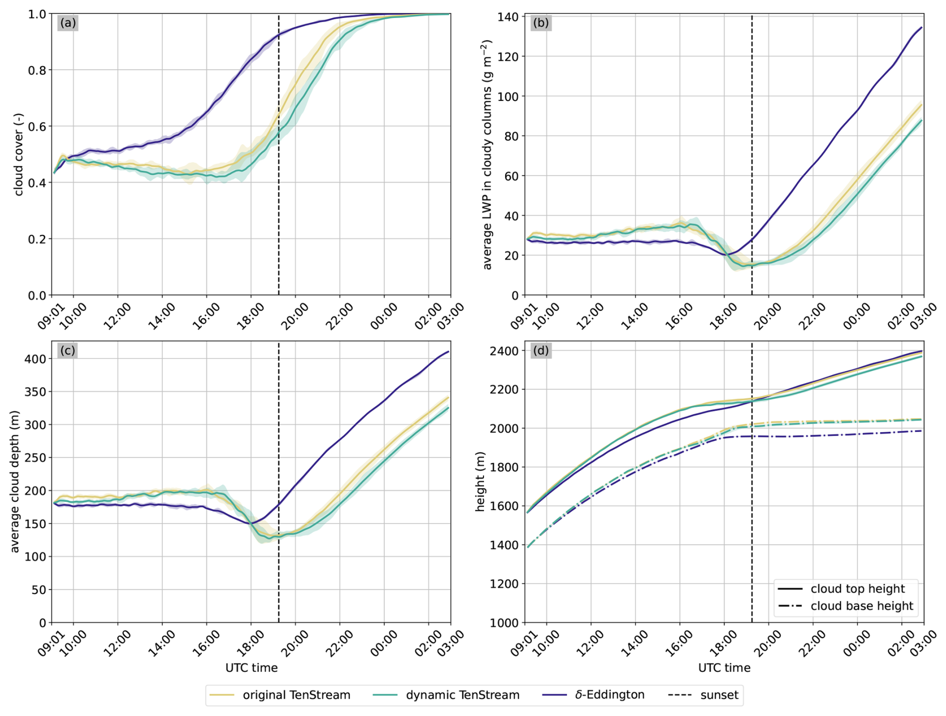
Figure 4 Temporal evolution of cloud cover (a), average liquid water path in cloudy columns (b), average cloud depth (c), and cloud top and base heights (d) for the restart simulations introduced in Sect. 2.1.4. The colored lines show the ensemble mean for each radiative transfer solver, while the shaded areas cover the minimum-to-maximum range across the corresponding five-member ensemble. The vertical line in all the panels marks the sunset time. To improve readability, a 15 min running mean was applied to the data before plotting.

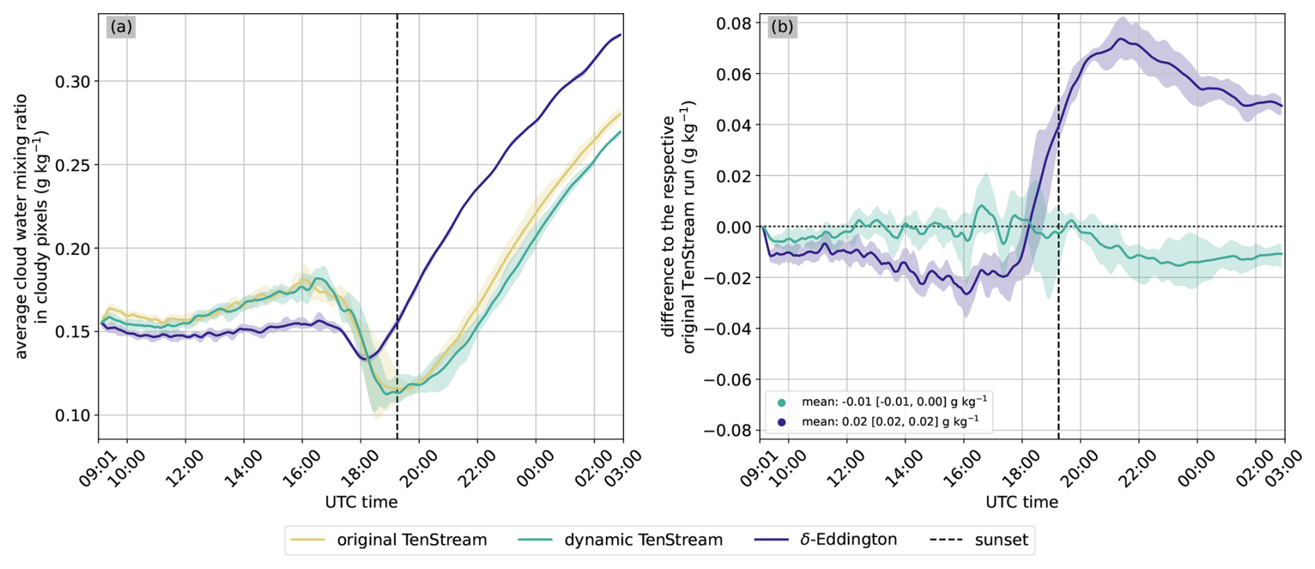
Figure 5 Temporal evolution of the average cloud water mixing ratio q_c in cloudy pixels (a) and differences relative to the corresponding TenStream reference run (b). As in Fig. 4, the colored lines show the ensemble mean for each radiative transfer solver, while the shaded areas indicate the corresponding ensemble spreads. The legend in panel (b) provides temporal mean differences and their minimum-to-maximum ranges. By isolating changes in in-cloud condensate from changes in cloud depth, this plot complements Fig. 4b. As in this preceding figure, the vertical line marks the time of sunset, and a 15 min running mean was applied to the data before plotting.

Apart from that, panels (b) and (c) show that the clouds in simulations coupled to 3D radiative transfer also become thicker and feature a higher average liquid water path during daytime than their 1D-driven counterparts, similar to what has been shown in other studies (Veerman et al., 2020, 2022; Tijhuis et al., 2024). Both effects are not very large, but the corresponding ensemble spreads do not overlap, and the differences are therefore robust compared to the intrinsic variability of the simulations. Quantitatively, the average LWP in cloudy columns during daytime is 25.7 [25.7, 25.8] g m⁻² in the δ-Eddington ensemble, whereas it is 29.0 [28.5, 29.8] g m⁻² in the dynamic TenStream ensemble and 29.6 [29.2, 30.2] g m⁻² in the original TenStream ensemble. Here and in the following, values are reported as ensemble means, with the minimum and maximum temporal averages across the five ensemble members given in square brackets. In terms of average cloud depth during daytime, these values are given by 172 [172, 173], 181 [180, 184], and 184 [183, 186] m, respectively. Hence, the clouds in the simulations coupled to 3D radiation are about 5  %–7  % thicker and feature an LWP larger by about 13  %–15  % during the day. As shown in Fig. 5, this increase in LWP is also not only caused by the increased depth of the clouds, but also by a higher overall cloud water mixing ratio, i.e., more liquid water per kilogram of air in the clouds coupled to 3D radiation.

Switching to nighttime, panel (a) of Fig. 4 shows that all simulations converge toward a completely overcast sky after sunset. However, the corresponding increase in cloud cover occurs significantly earlier in the 1D simulations. Alongside this, the cloud characteristics change substantially. Now, it is the clouds coupled to 1D radiation that become thicker and contain more liquid water. As shown in panel (d) of Fig. 4, this increased thickness is primarily due to the cloud base height stabilizing earlier in the 1D simulations, while the cloud top height develops similarly across all simulations. Together, this results in thicker clouds in the simulations driven by 1D radiation, although the development at night itself is not much different from the other simulations. Hence, the thicker clouds at night might actually be related to the higher cloud cover before sunset and the correspondingly reduced radiative energy at the surface, which could lead to an earlier suppression of convection. However, similar model runs with lower initial soil moisture, which did not feature a comparable increase in cloud cover near sunset, still lead to the development of the same nighttime cloud characteristics, i.e., the development of thicker clouds that contain more liquid water in simulations coupled to 1D radiative transfer, which suggests that these features are fairly robust overall.

Up to this point, the discussion has primarily focused on differences between simulations driven by 1D and 3D radiative transfer. We now turn to the second objective of this study, namely whether the incomplete solves in the dynamic TenStream solver can adequately reproduce these 3D-related differences. Revisiting Fig. 4, panels (a)–(c) show that the cloud characteristics generally agree well between the dynamic and original TenStream solvers, although small differences occur between daytime and nighttime. During the day, the clouds driven by the two solvers exhibit nearly identical characteristics, with overlapping ensemble spreads. At night, however, the dynamic TenStream solver slightly underestimates cloud cover, average liquid water path in cloudy columns, and average cloud depth. Nonetheless, these discrepancies remain small compared to the differences between the δ-Eddington and TenStream reference ensembles and suggest that the incomplete solves effectively capture all relevant 3D-related effects in terms of cloud characteristics.

It is important to note, however, that the performance of the dynamic TenStream solver is highly dependent on the simulation setup, and particularly on factors such as resolution, domain decomposition, and cloud cover. The relatively high cloud cover in the simulations here, for example, is very beneficial for its performance, as the clouds are relatively close to each other. This proximity reduces the distance – measured in grid boxes – over which information crucial for 3D radiative transfer must be transported. When the overall cloud cover drops below 30 % – which is common for shallow cumuli, with Neggers et al. (2003), for instance, reporting cloud covers between 10 % and 20 % on a prototypical shallow cumulus day – the performance of the solver weakens, as the increased spacing between clouds requires information to traverse more grid boxes, and potentially even multiple subdomains. At this point, performing just two Gauß–Seidel iterations per radiation scheme call may not be sufficient anymore. However, the dynamic TenStream solver was developed with NWP models in mind. At their kilometer-scale resolution, clouds are inherently closer together in terms of grid box distance, which should significantly mitigate this issue.

3.3 Differences in cloud–radiation interactions

So far, the analysis has primarily focused on the different development of clouds in simulations driven by 1D and 3D radiative transfer, showing that the dynamic TenStream solver successfully captures most of the 3D effects on clouds, despite relying on incomplete solves. However, the causes of these differences have not yet been investigated. Identifying them is challenging, as the clouds in the fully interactive PALM simulations are not only shaped by the corresponding radiative fields but also actively influence them, making it difficult to separate cause from effect. Nevertheless, this subsection still aims to identify at least some of the connections between the different radiative fields and the resulting cloud characteristics. In doing so, the following subsubsections will all follow the same overall structure: first, they will examine how treating radiation in 3D rather than 1D affects cloud development; then, they will assess whether the dynamic TenStream solver is also able to capture these effects.

3.3.1 Positioning of the clouds relative to their shadows

Before discussing the first way in which the different treatment of radiation in the 1D and 3D simulations affects the resulting cloud characteristics, let us briefly summarize the differences in the corresponding net solar surface irradiance fields. As shown in Fig. 6, these fields differ quite substantially between the simulations driven by 1D radiation (left panels) and those driven by 3D radiative transfer (middle and right panels). With 1D radiation, cloud shadows – the areas with low net solar surface irradiance – are positioned directly beneath the corresponding clouds, while the cloud-free columns around these shadows are all subject to very similar clear-sky conditions, resulting in the relatively uniform background color in these panels. With 3D radiation, by contrast, cloud shadows are displaced according to the angle of solar incidence. In addition, the net solar surface irradiance is lower within these shadows, which is due to the thicker clouds that contain more liquid water in these simulations, as well as generally darker cloud shadows in simulations coupled to 3D radiation (e.g., Gristey et al., 2020). Even more striking in the 3D simulations are the bright areas at the sunward edges of the shadows, which appear, for example, to the east of the shadows in panel (c) and to the west of them in panel (l), with the Sun positioned at azimuth angles of 121° (i.e., in the east–south–east) and 262° (i.e., in the west), respectively. These so-called cloud enhancements (Tijhuis et al., 2022) occur because radiation escaping through cloud sides or entrapped between the surface and the cloud base enhances the diffuse downward radiation (Hogan and Shonk, 2013; Hogan et al., 2019).

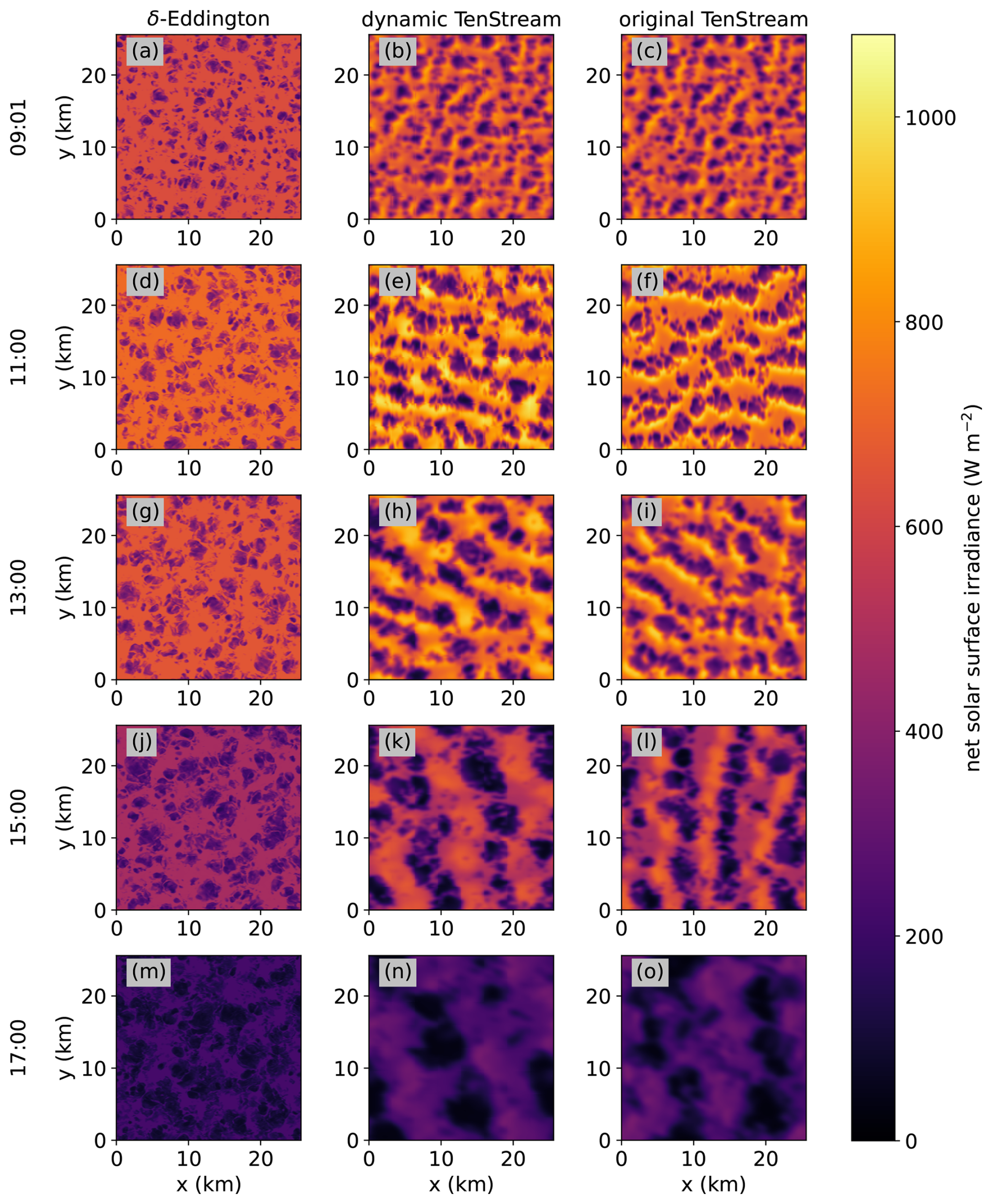
Figure 6 Temporal evolution of the net surface irradiance in the solar spectral range for the simulations driven by the δ-Eddington approximation (left), the dynamic TenStream solver (middle), and the original TenStream solver (right), shown for five time steps between 09:01 and 17:00 UTC. Only simulations performed from the main run of the setup are shown.

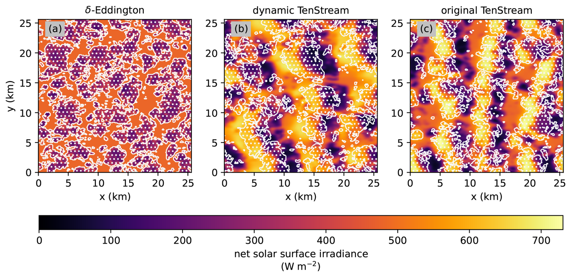
Figure 7 Positioning of the clouds relative to the net solar surface irradiance fields at 15:00 UTC in the simulations coupled to the δ-Eddington (a), dynamic TenStream (b) and original TenStream (c) solvers. To this end, the white contour lines in each plot enclose areas where the vertical columns above each grid point contain at least one grid box with q_c>0.01 g kg⁻¹, classifying them as cloudy. To improve the overall contrast of the plots, the maximum value of the colorbar was set to the highest net surface irradiance across the three panels, rather than the global maximum from all simulations, as it was done in Fig. 6.

Now, let us examine how these differently structured fields might relate to the differences in cloud characteristics observed in Sect. 3.2. To this end, we compare panels (j)–(l) in Fig. 6 with panels (g)–(i) in Fig. 3. Figure 7 facilitates this comparison by projecting the outlines of the corresponding clouds onto the underlying net surface irradiance fields. As we can see in panel (a) of that figure, with 1D radiation, the cloud shadows are unsurprisingly placed directly below the corresponding clouds. This placement of shadows, however, suppresses the updrafts responsible for cloud formation, thereby reducing both the size and lifetime of the clouds (e.g., Schumann et al., 2002; Horn et al., 2015). In contrast, the original TenStream solver in panel (c) shows a displacement of the shadows to the east of the corresponding clouds. Beneath them, we instead observe regions of increased net surface irradiance that even exceed the clear-sky values in panel (a). These regions, in turn, likely strengthen, rather than weaken, the corresponding updrafts, potentially explaining why the clouds coupled to 3D radiation are larger and thicker than those in the 1D simulation during daytime.

Ultimately, this hypothesis is difficult to prove, as the clouds are not only shaped by the corresponding radiative fields but also actively influence them through their evolving characteristics. However, at least some evidence that the observed changes in cloud characteristics are primarily driven by the radiative field can be found in panels (a)–(c) of Fig. 6, where the clouds have not yet evolved but are already subject to the discussed effects. Of course, this is not enough to prove our hypothesis, though. Similar challenges associated with the coupling of radiation and model dynamics were also highlighted by Tijhuis et al. (2024), who investigated a similar hypothesis. They came to comparable conclusions, although their more statistical approach found the wind–sun angle to be an even more important factor for the development of larger and thicker clouds during daytime than just the shadow displacement. The mechanism behind this dependence on the wind–sun angle is that clouds driven by 3D radiation cannot significantly outgrow their 1D counterparts if they move into their own shadows, as this suppresses their updrafts, similar to what occurs in 1D simulations. Conversely, if the clouds do not move into their own shadows, the updrafts can persist or even intensify, allowing the clouds to live longer and grow larger (Tijhuis et al., 2024). In the qualitative analysis presented here, no such strong dependency on the wind–sun angle is observed, since the clouds continue to grow even when moving into their own shadows, as can be seen starting with the panels at 13:00 UTC in Fig. 6. However, this does not necessarily negate the existence of this mechanism. Instead, it suggests that in our simulations, the surface response to cloud movements is sufficiently rapid to maintain the updrafts in sunlit regions. This is consistent with the surface skin-layer heat capacity of C₀=0 J m⁻² K⁻¹ used in these simulations, which causes an instantaneous adjustment of the surface energy budget to changes in the radiative field. Otherwise, the results align with those of Tijhuis et al. (2024), although the connection between the clouds and areas of increased net surface irradiance has been emphasized much more strongly here. The representation of these cloud–enhanced areas relies on unique 3D effects, such as cloud–side escape (Hogan and Shonk, 2013) and entrapment (Hogan et al., 2019), which can only be accounted for with full 3D radiative transfer, underscoring the importance of 3D radiative transfer for the correct representation of cloud characteristics in numerical models.

Having discussed this first effect of 3D radiation on cloud characteristics, let us now turn to the second objective of this study, namely whether the incomplete solves in the dynamic TenStream solver can also capture this effect. To this end, we first consider the middle panels of Fig. 6, which show that the dynamic TenStream solver is indeed able to reproduce most of the features of the original TenStream solution, although it slightly overestimates the spatial extent of the cloud enhancements. This overestimation can be at least partially attributed to the delayed interaction between the radiative fluxes at the clouds and the surface when using incomplete solves, especially when this interaction spans multiple subdomains. In such cases, radiative enhancements caused by a cloud may persist at a specific location on the ground even after the cloud has moved on with the mean wind flow, thereby enlarging the associated features on the surface. Following this reasoning, these artifacts are expected to be most pronounced when the solar zenith angle is large, resulting in interactions that involve multiple subdomains, and when the clouds move away from the direction of solar incidence and thus away from their radiatively enhanced areas. And indeed, the overestimation is relatively small in panel (b), where the clouds are moving toward the Sun, but becomes much more pronounced in panel (k), where the Sun is at a zenith angle of 51° and the clouds move away from the direction of solar incidence, allowing the cloud-enhancement areas to increase in size.

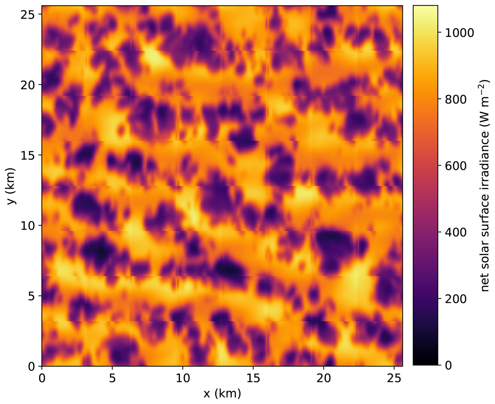
Figure 8 Magnified version of panel (e) in Fig. 6, highlighting the discontinuities between subdomains in the dynamic TenStream solver.

Apart from this, the dynamic TenStream net solar surface irradiance fields feature another artifact that becomes visible in magnified views. Figure 8 provides such a close-up for panel (e) of Fig. 6. In this magnification of the net surface irradiance field, one can clearly see the underlying domain decomposition into 8 × 8 subdomains through discontinuities at the respective subdomain boundaries. These discontinuities occur because the incomplete solves in the dynamic TenStream solver are performed independently for all subdomains, with interactions between them taking place only once at the end of each radiation scheme call. As a result, the individual subdomains have not yet updated their radiative fluxes based on the new boundary conditions at the end of each call, leading to the observed artifacts. However, these discontinuities are relatively small and, for this setup, do not significantly affect the representation of any of the 3D effects discussed previously.

Since all the main features of the original TenStream fields are thus captured by the dynamic TenStream solver, we can now turn to Fig. 7 to investigate whether, similar to the original TenStream run, the clouds in the dynamic TenStream simulation are also maintained over regions of enhanced net surface irradiance. And indeed, we can observe a similar positioning of the clouds relative to their shadows, which are displaced to the east as a physical 3D radiative-transfer effect also in the dynamic TenStream simulation. In contrast to the original TenStream simulation, however, the regions of enhanced net surface irradiance are less concentrated underneath the clouds and appear spatially broader in the dynamic TenStream simulation. This broadening of the radiatively enhanced areas has already been discussed and can be attributed to the incomplete solves, which delay the interaction between radiative fluxes at the clouds and the surface. Specifically, as the clouds move eastward, both the response of the surface to the clouds and the subsequent radiative feedback from the surface back to the clouds can lag behind. Despite this lag, however, substantial portions of the clouds remain positioned over regions of increased net surface irradiance. Thus, also in the dynamic TenStream simulations, the surface irradiance pattern likely strengthens rather than weakens the corresponding updrafts, thereby promoting the observed differences in cloud characteristics.

3.3.2 Differences in the surface energy budget

Up to this point, our analysis has primarily focused on differences in the spatial structure of the net surface irradiance fields and their potential relation to the differences in cloud characteristics observed in Sect. 3.2. What remains to be investigated, however, is whether the simulations coupled to the δ-Eddington approximation exhibit systematic biases when compared to the TenStream reference solution. To investigate this aspect as well, we turn to Fig. 9, where panel (a) illustrates the temporal evolution of the domain-averaged net surface irradiance presented in Fig. 6. Despite the substantial differences in the spatial structure of the corresponding fields, these domain averages evolve quite similarly in the 1D and 3D simulations. Panel (c) quantifies the deviations from the corresponding TenStream reference run, showing that for most of the day, the δ-Eddington runs differ by less than 10 W m⁻² from the reference solution. It is only after about 14:00 UTC that they become subject to larger deviations, peaking at around 30 W m⁻². However, going back to Fig. 4, we can see that this divergence coincides with a noticeable increase in cloud cover in the 1D simulations after 14:00 UTC, which naturally reduces the net surface irradiance compared to the 3D simulations, where the cloud cover remains lower. Apart from this specific difference, we can conclude that no substantial bias is introduced into the domain-averaged net solar surface irradiance when using 1D instead of 3D radiative transfer.

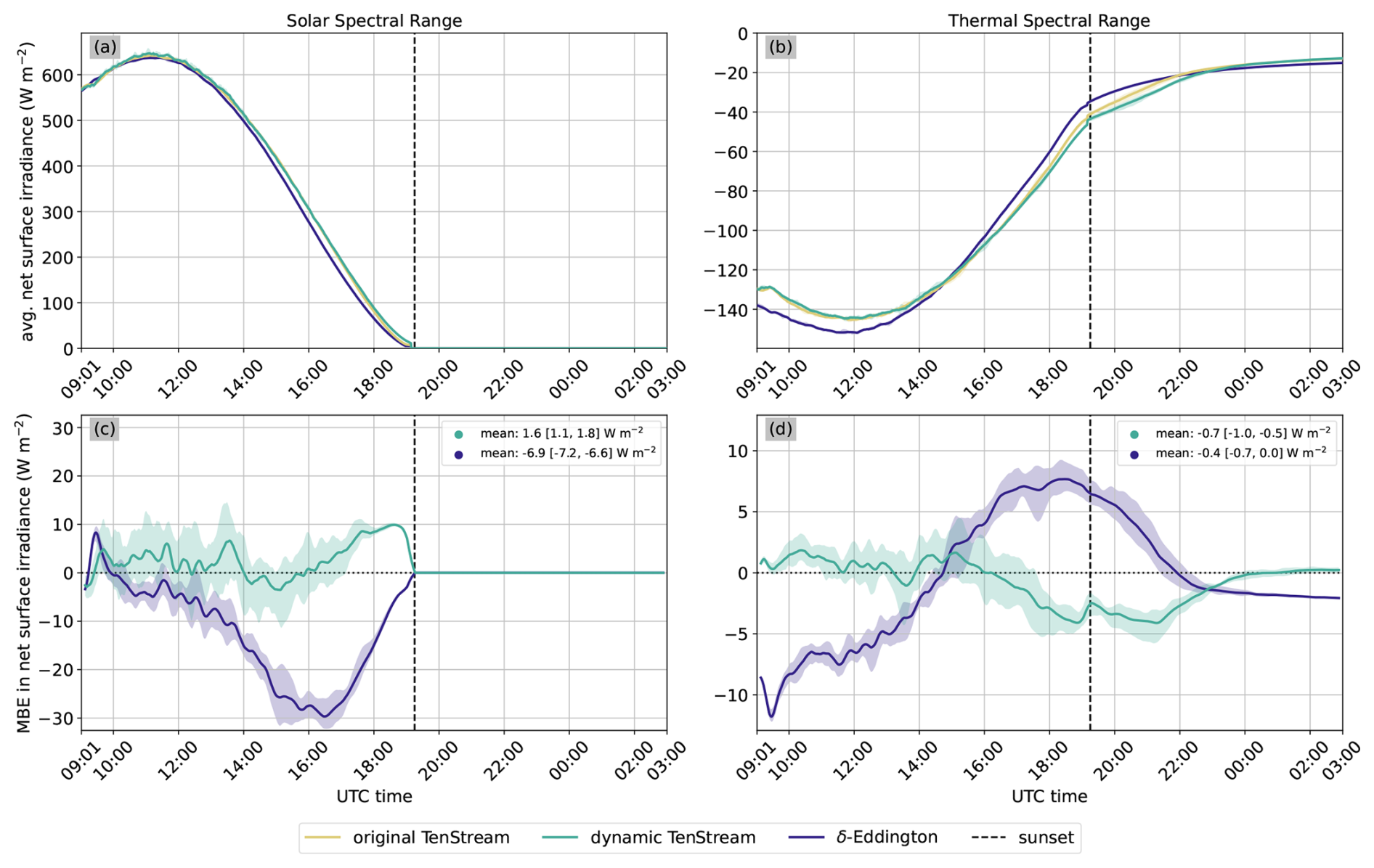
Figure 9 Temporal evolution of the domain-averaged net surface irradiance in the solar (a) and thermal (b) spectral ranges for the three five-member ensembles discussed in this paper. Panels (c) and (d) show the corresponding differences relative to the respective TenStream reference run. In all panels, the colored lines show the ensemble mean for each radiative transfer solver, while the shaded areas indicate the corresponding ensemble spreads. The legends in panels (c) and (d) provide temporal mean differences and their minimum-to-maximum ranges. To improve readability, a 15 min running mean was applied to the data in panels (c) and (d) before plotting. The vertical line in each panel marks the time of sunset.

This small domain-averaged difference is consistent with findings in previous studies. As illustrated in Fig. 10 of Maier et al. (2024), 1D radiative transfer, when applied to a prescribed cloud field, tends to underestimate the net surface irradiance at small solar zenith angles, as it cannot account for cloud-side escape and entrapment, which both enhance the diffuse downward radiation. Conversely, at large solar zenith angles, 1D solvers typically overestimate the net surface irradiance because they cannot cast shadows at slant angles, thereby underestimating their size. In the fully interactive PALM simulations, however, especially the underestimation at small solar zenith angles is counteracted by the development of larger and thicker clouds in the 3D simulations, which increase absorption and backscattering to space, as explained in Tijhuis et al. (2024). As a result, and consistent with their findings, no substantial differences in the domain-averaged net surface irradiance are observed between simulations coupled to 1D and 3D radiation. This underscores that, at least in the solar spectral range, 3D radiative transfer is primarily important to accurately model the spatial structure of the radiative fields. However, it does not substantially affect the domain-averaged properties of these fields.

This is slightly different in the thermal spectral range. Panel (b) of Fig. 9 shows the temporal evolution of the domain-averaged net surface irradiance for the different simulations in this spectral range. We can see that initially, the simulations coupled to 1D radiation experience systematically stronger cooling, similar to what was observed in Fig. 9 of Maier et al. (2024). This is most likely because the increased thermal emission of clouds affects not only the cloudy columns themselves when using 3D radiative transfer, but also neighboring ones due to the horizontal transport of energy in these solvers. Especially early on, when the surface temperature – which primarily determines the upward thermal irradiance at the surface – is still similar across all simulations, the correspondingly increased downward irradiance at the surface is likely the main factor explaining the systematically weaker net cooling observed with 3D radiation. This pattern changes, however, at around 15:00 UTC, when the cloud cover in the 1D simulations noticeably increases. Along with this shift in cloud cover, the net thermal emission in the 1D simulations decreases and becomes lower than in the 3D simulations. As shown in Fig. 16 of Maier et al. (2024), net thermal emission is significantly reduced below clouds when using 1D radiative transfer, explaining this noticeable decrease in net thermal emission as the cloud cover starts to rise.

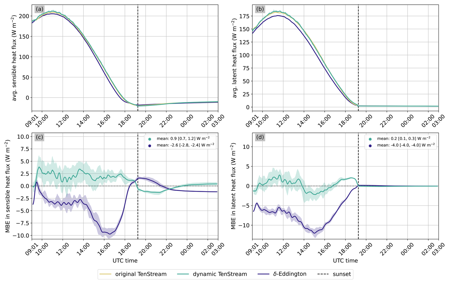
Figure 10 Temporal evolution of the domain-averaged sensible (a) and latent (b) heat fluxes for the three five-member ensembles discussed in this paper. Panels (c) and (d) show the corresponding differences relative to the respective TenStream reference run. In all panels, the colored lines show the ensemble mean for each radiative transfer solver, while the shaded areas indicate the corresponding ensemble spreads. The legends in panels (c) and (d) provide temporal mean differences and their minimum-to-maximum ranges. To improve readability, a 15 min running mean was applied to the data in panels (c) and (d) before plotting. The vertical line in each panel marks the time of sunset.

Since the temporal evolution of the domain-averaged net solar surface irradiance showed only minor differences between the 1D and 3D solvers, the observed differences in the domain-averaged net thermal surface irradiance are expected to be compensated by changes in other components of the surface energy budget. In general, the net solar irradiance at the ground is balanced by net thermal emission, the ground heat flux, and the release of sensible and latent heat into the atmosphere. Hence, the observed differences in the net thermal irradiance can result in changes in any of the latter three components. To investigate which of them compensates for the observed differences, Fig. 10 illustrates the temporal evolution of the sensible and latent heat fluxes across the three solver ensembles considered in this evaluation. Looking at panels (a) and (b), first note that the Bowen ratio – i.e., the ratio of the sensible to the latent heat flux (Bowen, 1926) – is larger than one in all simulations. This is rather unusual for vegetated surfaces such as the flat grassland used here, and more characteristic of urban environments or semi-arid regions (e.g., Stull, 2006; Kotthaus and Grimmond, 2014), suggesting that the soil in the model is relatively dry. Apart from this general remark, panel (a) of Fig. 10 shows that the sensible heat flux evolves quite similarly across all simulations until about 15:00 UTC. At that point, the simulations coupled to 1D radiation begin to slightly diverge from those using 3D radiation. As discussed earlier, this divergence coincides with a substantial increase in cloud cover in the 1D simulations at that time, subsequently leading to a reduction of the net solar surface irradiance. Panel (a) indicates that this reduction in solar energy input also affects the release of sensible heat into the atmosphere, which is subsequently reduced by up to 10 W m⁻² in the 1D simulations, as can be seen in panel (c).

A much more striking difference between the 1D and 3D simulations is revealed in panel (b), which shows that the domain-averaged latent heat flux is considerably higher in the simulations coupled to 3D radiation, accompanied by a slightly faster decrease in soil moisture (not shown here). This finding suggests that the reduced thermal emission in the 3D simulations observed in Fig. 9 – which could be balanced by a decrease in net solar irradiance, or by increases in the ground, sensible, or latent heat fluxes, or a combination thereof – is primarily offset by an increased release of water vapor into the atmosphere. In PALM, this latent heat flux is parameterized as

$$\begin{array}{}\text{(3)}& {\displaystyle }LE=-{\displaystyle \frac{\mathit{\rho }{l}_{\mathrm{v}}}{r_{\mathrm{a}}+r_{\mathrm{s}}}}\left[q_{\mathrm{v}}\left({\displaystyle \frac{\mathrm{\Delta }z}{\mathrm{2}}}\right)-q_{\mathrm{v},\mathrm{sat}}\left(T_{\mathrm{0}}\right)\right],\end{array}$$

where ρ is the density of dry air, $l_{\mathrm{v}}=\mathrm{2.5}\times {\mathrm{10}}^{\mathrm{6}}$ J kg⁻¹ is the specific latent heat of vaporization, r_a and r_s are the aerodynamic and surface resistances (in units of s m⁻¹), $q_{\mathrm{v}}\left(\frac{\mathrm{\Delta }z}{\mathrm{2}}\right)$ is the water vapor mixing ratio at height $z=\frac{\mathrm{\Delta }z}{\mathrm{2}}$, with Δz denoting the vertical grid spacing, and q_v, sat(T₀) is the saturation vapor mixing ratio at the radiative temperature T₀ of the surface skin layer (Maronga et al., 2020). Since the differences in the domain-averaged $q_{\mathrm{v}}\left(\frac{\mathrm{\Delta }z}{\mathrm{2}}\right)$ relative to the corresponding TenStream reference runs remain below 0.8  % for both the δ-Eddington and dynamic TenStream simulations, even when considering their full ensemble spreads (not shown here), the enhanced latent heat flux in the 3D simulations is unlikely to be driven by changes in near-surface humidity. Instead, it is most consistent with an increase in q_v, sat(T₀), and thus in the radiative temperature T₀ of the surface skin layer. In PALM, such an increase in T₀ is governed by imbalances in the ground energy budget, following the relationship

$$\begin{array}{}\text{(4)}& {\displaystyle }{C}_{\mathrm{0}}{\displaystyle \frac{\mathrm{d}{T}_{\mathrm{0}}}{\mathrm{d}t}}=R_{\mathrm{n}}-H-LE-G,\end{array}$$

where C₀ denotes the heat capacity of the surface skin layer (in units of J m⁻² K⁻¹), R_n is the net radiative intake at the surface, H is the sensible heat flux, and G is the ground heat flux (Maronga et al., 2020). In the 3D simulations, R_n is increased across both spectral ranges, while H, LE, and G initially remain unchanged. This is consistent with an increase in T₀ in these simulations, which subsequently leads to increases in H, LE, and G. Since q_v, sat is directly proportional to the saturation vapor pressure $e_w^{*}$, which itself depends exponentially on T₀, even small increases in T₀ can lead to substantial increases in q_v, sat(T₀) and, consequently, in LE, explaining why the elevated skin layer temperature affects the latent heat flux more strongly than the sensible one. Moreover, this relationship supports the interpretation that the higher latent heat fluxes in the 3D simulations are primarily driven by increases in q_v,sat(T₀), since changes in the aerodynamic resistance r_a – which could also affect LE – would tend to affect both H and LE more uniformly. Overall, the increased latent heat flux in the 3D simulations provides another potential explanation for why clouds grow thicker and larger during the day than their 1D-driven counterparts, as more water vapor is released into the atmosphere with 3D radiation. In contrast to the previously discussed mechanism related to the positioning of clouds relative to their shadows and sunlit regions, this longwave-driven effect has, to our knowledge, not been described in the literature before.

Having discussed this second effect of 3D radiation on cloud characteristics, we now return to the second objective of this study and assess whether the incomplete solves in the dynamic TenStream solver can also capture this effect. First, going back to Fig. 9c, we can see that the domain-averaged net solar surface irradiance in the dynamic TenStream ensemble differs by less than 10 W m⁻² from the original TenStream ensemble throughout most of the simulation. In particular, no significant accumulation of bias over time is observed when using the dynamic TenStream solver, in contrast to the findings of Maier et al. (2024). It should be noted, however, that in their Fig. 9 this bias accumulation mostly remained below 10 W m⁻², and hence within the variability of the bias seen in panel (c) of Fig. 9. The domain-averaged net thermal surface irradiance also shows only small deviations from the original TenStream ensemble, with differences remaining below 5 W m⁻² throughout the entire simulation, as shown in panel (d) of Fig. 9. This indicates that the dynamic TenStream solver, despite its use of incomplete solves, is still able to capture all the key features of the full 3D solution, especially the initially weaker net thermal cooling compared to the δ-Eddington ensemble. Looking at Fig. 10, we can further see that, as in the original TenStream ensemble, this reduced domain-averaged net thermal emission in the dynamic TenStream ensemble is primarily balanced by an increased latent heat flux. Deviations from the TenStream reference solution remain below 5 W m⁻², compared to deviations of more than 10 W m⁻² for the 1D simulations. Thus, like the original TenStream solver, the dynamic TenStream solver is able to capture the enhanced latent heat flux in the simulations driven by 3D radiative transfer and, with it, the second potential explanation for why clouds driven by 3D radiation grow thicker and larger during the day than their 1D-driven counterparts.

3.3.3 Summary and limitations

In summary, two potential links have now been identified between radiation and cloud characteristics that help explain why clouds in simulations coupled to 3D radiative transfer grow larger, become thicker, and contain more liquid water during the day than their 1D-driven counterparts:

1. First, clouds in simulations coupled to 3D radiative transfer were found to be positioned above areas of increased net surface irradiance, rather than above their own shadows. This placement causes the associated updrafts to persist or even strengthen instead of weakening.

2. Additionally, 3D radiative transfer reduces the domain-averaged net thermal emission at the ground, most likely because the stronger thermal emission from clouds enhances the downward longwave radiation not only in cloudy, but also in neighboring columns. This reduction in net thermal surface irradiance affects the ground energy budget and appears to be primarily balanced by an increase in the domain-averaged latent heat flux, resulting in a greater release of water vapor into the atmosphere.

The relative importance of these two effects, i.e., the extent to which each of them contributes to the observed changes in cloud characteristics, however, has not yet been investigated. Quantifying their individual contributions would require additional sensitivity experiments, for example simulations in which 3D radiative transfer is applied only in the solar or only in the thermal spectral range. Such simulations would make it possible to assess how much the longwave-driven surface-energy-budget effect contributes relative to the positioning of clouds within the net solar surface irradiance fields. More important for the present study, however, is that both effects are captured not only by the full original TenStream model but also by the dynamic TenStream solver. This demonstrates that the incomplete solves in the latter provide a computationally efficient approach that not only captures the essential features of 3D radiative fields, but also reproduces most of the resulting cloud characteristics in fully interactive PALM simulations. These include the development of larger and thicker clouds containing more liquid water during the day, as well as thinner clouds with less liquid water at night. The causes of these nighttime cloud characteristics, however, are more difficult to disentangle and would require additional experiments, such as restarting the simulations at sunset, to separate the imprint of daytime evolution from genuinely nocturnal radiative effects, which is beyond the scope of this study.

Finally, it should also be noted that the original TenStream solver used as a reference in this paper is an approximation itself. The differences between this approximation and highly accurate 3D radiative transfer solvers such as the Monte Carlo model MYSTIC have been discussed in Maier et al. (2024) and are mostly much smaller than the 3D radiative effects and their subsequent influences on cloud development observed in this paper. Especially the results during daytime have furthermore been shown to be in good agreement with those of Tijhuis et al. (2024), which were obtained with a GPU-accelerated Monte Carlo ray tracer. Thus, while the exact magnitude of some of the effects discussed in this paper might slightly vary when using a highly accurate 3D radiative transfer model such as MYSTIC, the key features and underlying mechanisms are expected to remain unchanged.

4 Summary and outlook

The primary objective of this paper was to investigate how coupling the dynamic TenStream solver to model dynamics affects cloud development and how the resulting clouds compare to those driven by classical 1D and full 3D radiation. To answer these questions, PALM (Raasch and Schröter, 2001; Maronga et al., 2015, 2020) was used to perform a large-eddy simulation (LES) in which shallow cumulus clouds developed over the course of the day. Once the clouds had formed, three restart runs of the simulation were conducted, each coupled to a different radiative transfer model: either a classical 1D δ-Eddington approximation, the original TenStream model, or the new dynamic TenStream solver. Starting from the same cloud field, this setup then enabled a direct comparison of how the simulated clouds evolved depending on the radiative transfer model used. To analyze the differences between the three simulations, daytime and nighttime conditions were considered separately. During the day, the clouds in the dynamic and full TenStream simulations were shown to organize into cloud streets aligned perpendicular to the angle of solar incidence, extending the findings of Jakub and Mayer (2017) to a realistic diurnal cycle in which the cloud streets follow the changing azimuthal position of the Sun. With 1D radiation, on the other hand, the clouds remained more or less randomly positioned. Clouds driven by the two 3D solvers were also shown to grow larger, become thicker, and contain more liquid water than those coupled to 1D radiation, in agreement with Veerman et al. (2020, 2022) and Tijhuis et al. (2024). After sunset, however, this pattern reversed, with the clouds in the 1D simulation becoming thicker and containing more liquid water than their 3D-driven counterparts. Throughout both day and night, the dynamic TenStream solver successfully captured all these 3D effects, with discrepancies from the original TenStream model remaining small compared to the differences observed for the 1D simulation. In contrast to these averaged cloud characteristics, the positioning of individual clouds in the dynamic and full TenStream simulations, however, indeed differed over time, illustrating that even the small differences in their corresponding radiative fields influenced individual cloud development over time, despite sharing very similar overall characteristics.

Building on these observations, this paper then sought to identify the mechanisms driving the described differences in cloud characteristics, with a particular focus on the daytime regime. A comparison of the corresponding net solar surface irradiance fields revealed first key differences. As expected, cloud shadows in the 3D simulations were displaced according to the angle of solar incidence, in contrast to the 1D simulation, where they were positioned directly beneath the corresponding clouds. At the sunward edges of the shadows, furthermore, areas of enhanced net surface irradiance were identified in the 3D simulations, with values even exceeding those in the clear-sky columns of the 1D simulation. Unlike their 1D-driven counterparts, the clouds in the 3D simulations turned out to be located above these areas of enhanced net surface irradiance. Similar to the mechanism described by Tijhuis et al. (2024), this positioning of the clouds likely caused the associated updrafts to persist rather than weaken, promoting the observed differences in cloud characteristics. In addition, 3D radiative transfer was found to reduce the domain-averaged net thermal emission at the ground, most likely because the stronger thermal emission from clouds enhances the downward longwave radiation not only in cloudy, but also in neighboring columns. This reduction in net thermal surface irradiance affected the ground energy budget in these simulations and appeared to be primarily balanced by an increase in the domain-averaged latent heat flux, resulting in a greater release of water vapor into the atmosphere. To our knowledge, this represents a second effect of 3D radiation on cloud characteristics that has not yet been described in the literature. Together, both effects helped explain why clouds in the 3D simulations grew larger, became thicker, and contained more liquid water during the day than those in the 1D simulation, although their relative contributions remain to be investigated. Importantly, both the original TenStream model and the dynamic TenStream solver captured these effects, further underscoring the latter's ability to represent 3D radiative effects on cloud development at a significantly lower computational cost.

It should be noted, however, that this study focused exclusively on shallow cumulus clouds with a relatively high cloud cover of more than 40 %. In reality, though, clouds occur in a wide variety of forms. On the one hand, there are clear-sky or completely overcast situations, which are essentially one-dimensional, with little to no horizontal variability and thus negligible 3D radiative effects. Multi-layer cloud fields and deep convection, on the other hand, represent more complex scenarios than the shallow cumulus clouds discussed here, as their larger vertical extent introduces radiative interactions across greater distances. Such cloud fields may therefore pose a stronger challenge for the incomplete solves in the dynamic TenStream solver. However, since all vertical layers above a given grid point belong to the same model subdomain, these vertical interactions can still occur within a single call to the radiation scheme even with incomplete solves, alleviating these concerns to some extent. This is not necessarily the case for cloud fields with different cloud covers. As discussed in Sect. 3.2, the relatively high cloud cover in this study, for example, likely favored the performance of the dynamic TenStream solver, because the clouds were close together in terms of grid-box distance, reducing the distance over which information crucial for 3D radiative transfer needed to be exchanged. Lower cloud covers, by contrast, increase this spacing and may thus weaken the solver’s performance. Future studies should therefore examine more diverse cloud configurations, including cases with more complex vertical structures and lower cloud cover, to evaluate the robustness of the solver under a wider range of conditions. These future studies could then also adopt more realistic simulation setups, including real-world initial profiles and external large-scale forcing, to assess the 3D radiative effects observed in this paper under more realistic dynamical conditions as well.

At this point it is also worth mentioning that while this work focused on high-resolution LES output, the dynamic TenStream solver was developed with numerical weather prediction (NWP) models in mind. At their current kilometer-scale resolution, clouds are inherently closer together in terms of grid-box distance, which should significantly mitigate the expected performance degradation in low-cloud-cover scenarios. In this regime, however, model grid boxes can no longer be treated as homogeneous, as it is currently assumed in the solver. Hence, the TenStream lookup tables used to determine the transport coefficients in the underlying system of linear equations will need to be extended to account for cloud fraction as well. In addition, although the dynamic TenStream solver is markedly faster than other 3D radiative transfer solvers, it remains about three times slower than a classical 1D δ-Eddington solver (Maier et al., 2024). Since a new radiative transfer scheme should ideally operate at a comparable cost to the 1D independent-column approximations employed in today's NWP models, further optimization is essential. One promising direction in that way would be to accelerate the retrieval of the transport coefficients from the TenStream lookup tables, which currently accounts for roughly one-third of the solver’s total runtime. Achieving such improvements would then finally enable the application of the dynamic TenStream solver at the scale it was originally intended for, paving the way toward addressing the open question of how 3D radiative transfer affects weather forecasts.