Cloud liquid water path at the North Slope of Alaska has minimal sensitivity to local meteorology in Arctic winter

Mixed-phase clouds in the Arctic are tightly coupled to the surface energy budget in the cold months, helping to set surface temperatures and sea ice extent. However, the meteorological conditions that give rise to these clouds and their remarkable persistence across the Arctic are not well constrained, leading to model biases. Using over a decade of observations from the North Slope of Alaska, this research investigates the relationships between cloud base temperature and moisture, bulk atmospheric moisture, wind direction, large-scale circulation, and cloud liquid and ice water path. Liquid-containing clouds are ubiquitous at this site, occurring 60 %–70 % of the time between November and March, although about one-third of those cases have a liquid water path under 10 g m⁻². We find that liquid water path is weakly sensitive to temperature and moisture and remarkably insensitive to wind direction and large-scale circulation. Furthermore, meteorological regimes with significant differences in temperature, moisture, and cloud fraction do not produce appreciable differences in cloud liquid water path. Ice water path, on the other hand, is clearly correlated with bulk atmospheric moisture, with particularly strong increases when precipitable water vapor exceeds the 90th percentile, and may be responsible for the muted response of liquid water path to high atmospheric moisture. To explain the observed sensitivity of ice water path and relative insensitivity of liquid water path to meteorology and large-scale circulation, we propose a series of hypotheses centered around a lack of dissipative mechanisms and the role of ice in enabling or limiting liquid mass accumulation.

1 Introduction

Clouds play a crucial role in Arctic climate. For most of the year, their longwave radiative surface warming effect outweighs their shortwave radiative cooling effect, leading to surface warming (Walsh and Chapman, 1998; Shupe and Intrieri, 2004; Stramler et al., 2011; Graham et al., 2017). These impacts are largely driven by liquid-containing or mixed-phase clouds, which have the strongest interaction with atmospheric radiation. Liquid-containing clouds are ubiquitous in the Arctic, occurring 20 %–50 % of the time even in winter over a wide range of environments (Mioche et al., 2015; Cesana et al., 2012; Shupe et al., 2006, 2011), making them a significant influence on surface conditions. Clouds influence the atmosphere itself as well, helping to cool and dry air masses that pass through polar regions (Ali and Pithan, 2020; Pithan et al., 2018). However, the Arctic is challenging and expensive to monitor, contributing to limited observations that nonetheless reveal large and persistent model biases across a wide range of environments, seasons, and meteorological conditions (Davy and Outten, 2020; Cai et al., 2021). Uncertainties around cloud processes and model representations have been identified as a major source of Arctic model biases (Medeiros et al., 2011; Pithan and Mauritsen, 2014; Solomon et al., 2023), leaving clouds a prime target for further study.

Arctic clouds form, persist, and eventually dissipate as part of a continuous process of air mass transformation. In polar regions, clouds are believed to play a particularly active role in the transformation of warm, moist mid-latitude air into cold, dry polar air (Cronin and Tziperman, 2015; Pithan et al., 2018; You et al., 2022). When a relatively warm, moist air mass is advected over a colder surface like polar sea ice or land, the near-surface air begins to cool, eventually reaching saturation to form clouds. Cloud liquid produces intense radiative cooling at cloud top while radiatively warming the surface to drive buoyant mixing, redistributing their radiative cooling and triggering a host of interacting processes (Morrison et al., 2012). Importantly, the liquid layers in these clouds are often the source of ice particle initiation, followed by rapid ice growth. Cloud ice is ultimately responsible for dissipating the cloud by precipitating out its moisture, although this can be a slow process due to weak precipitation and humidity inversions at cloud top that resupply fresh moisture through entrainment (Curry et al., 1988; Sedlar and Tjernström, 2009; Solomon et al., 2011). The air mass transformation framework suggests a kind of characteristic Arctic cloud lifecycle where warmer, moister air masses form clouds that eventually glaciate and leave behind colder, drier polar air, but observational evidence is limited and leaves many questions concerning how such transformations shape Arctic cloud occurrence.

Liquid-containing Arctic clouds can have lasting impacts on underlying surfaces. The presence or absence of liquid-containing clouds is one of the main distinguishing factors between the two states of the characteristic bimodal surface energy distribution that has been identified at many ground-based observatories across the Arctic (Stramler et al., 2011; Cox et al., 2012; Graham et al., 2017; Silber and Shupe, 2022; Solomon et al., 2023; Shupe et al., 2026; Shupe and Intrieri, 2004) as well as in satellite observations (Cesana et al., 2012; Bertossa and L’Ecuyer, 2024). By reducing energy lost from the surface, liquid-containing clouds increase surface temperature relative to clear sky conditions (Stramler et al., 2011; Graham et al., 2017). These impacts on temperature and downwelling radiation can lead to persistent changes in sea ice concentration and snow pack by altering the surface energy budget by tens of W/m² in crucial growth or melt periods (Zhang et al., 1996; Francis and Hunter, 2006; Maksimovich and Vihma, 2012; Philipp et al., 2020; Shupe et al., 2026). In an air mass transformation context, atmospheric rivers that inject heat and moisture from lower latitudes into the Arctic have been found to increase cloud fraction, cloud liquid, and cloud ice content, increase surface temperature by around 10 °C, and reduce sea ice concentration (You et al., 2022; Liu et al., 2018; Doyle et al., 2011; Woods et al., 2013; Pithan et al., 2018; Kirbus et al., 2023; Woods and Caballero, 2016). However, moisture intrusions represent an extreme perturbation, and it is unclear whether the relationship between atmospheric temperature and moisture and cloud properties also holds for more typical conditions.

In mixed-phase clouds containing both liquid and ice, the distribution of condensed mass into liquid and ice is complicated by interactions between the two. Between −38 and 0 °C, supercooled liquid droplets generally need to encounter ice nucleating particles (INPs) to initiate freezing (DeMott et al., 2010; de Boer et al., 2011), making liquid droplets nearly a prerequisite for forming ice. However, when ice and supercooled liquid coexist in the same volume, the difference in saturation vapor pressure between the two causes vapor to preferentially deposit on ice and evaporate from liquid, which can rapidly transfer mass from liquid to ice phase in the Wegener-Bergeron-Findeisen (WBF) process (Wegener, 1911; Bergeron, 1935; Findeisen, 1938). The effect of ice on liquid is particularly apparent in the seeder-feeder mechanism, in which ice crystals precipitating into a liquid-containing cloud layer tend to thin or even disperse that layer (Shupe et al., 2013; Korolev et al., 2017; Achtert et al., 2026) through the WBF mechanism and/or riming. How Arctic mixed-phase clouds regularly persist for hours and even days in spite of the WBF process is an enduring puzzle in Arctic cloud research (Morrison et al., 2012; Shupe, 2011; Zuidema et al., 2005; Verlinde et al., 2007). The WBF process, along with a host of other mechanisms including secondary ice production and riming (Field et al., 2017; Korolev and Leisner, 2020), serves to highlight the challenge of connecting the microscale to the macroscale and identifying the conditions that are favorable for cloud liquid versus cloud ice.

This study was designed to explore the influence of temperature, moisture, wind direction, and large-scale circulation on wintertime cloud phase with a particular focus on liquid water path using long-term measurements from the North Slope of Alaska. Since a moist adiabat ties condensed mass to cloud base conditions, we expected a strong relationship between liquid water path, cloud base temperature, and cloud depth. Given the response of cloud liquid to moisture intrusions, we anticipated a response to bulk atmospheric moisture as well. Additionally, an air parcel transformation framework suggests that air mass history, approximated by the circulation, may modify the liquid water path: whether a cloud layer is forming or dissipating, or how developed the ice production has become, for example. Instead, the observations presented here reveal a remarkable insensitivity of liquid water path to many meteorological controls. In this paper, we explore the relationships outlined above to develop hypotheses explaining the remarkable resilience of liquid-containing clouds in the Arctic.

2 Data & Methods

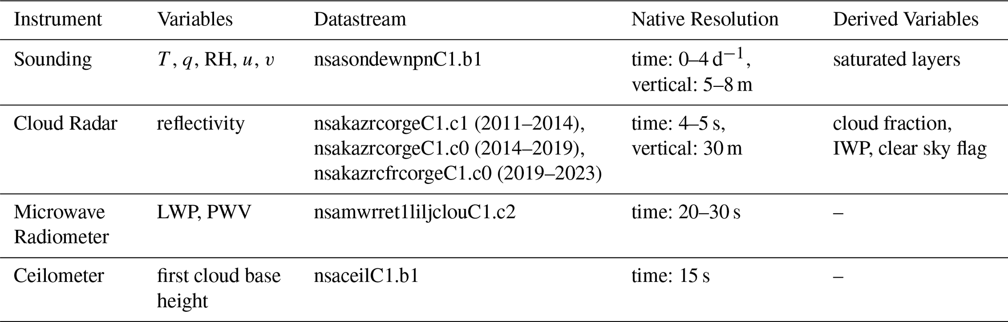
The primary data sources for this study are all taken from the North Slope of Alaska (NSA), a U.S. Department of Energy Atmospheric Radiation Measurement (ARM) User Facility (Verlinde et al., 2016). To maximize overlap between the different instruments while avoiding systematic biases from changes to specific instruments, the period from 12 November 2011 through 31 December 2023 is used for all ARM NSA data. An extended winter season is defined for this analysis, running from the start of November when the annual cycle of cloud fraction begins to decline to the end of March when it increases again each year (Shupe et al., 2011), and all data is restricted to this seasonal window. A summary of the instruments and their corresponding measurements used in this study is provided in Table 1 and described in detail below.

Table 1 Instrument & Dataset Details from North Slope of Alaska (ARM NSA). Datastream names are as they appear in the ARM data repository.

2.1 Radiosondes

Soundings are a backbone of this analysis. Radiosondes are released up to 4 times per day from NSA, and the resulting soundings are subject to quality checks run by ARM NSA on the Vaisala-processed temperature, humidity, wind direction, and wind speed to produce vertical profiles. For this analysis, these profiles are linearly interpolated onto a shared height coordinate from 0 to 12 000 m (all heights in this study are above ground level) in 5 m increments and each sounding is assigned a timestamp corresponding to the launch time of the radiosonde. Using extended winter data from 2011 through 2023 results in 4791 valid soundings after dropping the handful that did not report data up to at least 1000 m.

Saturated layers, a proxy for regions containing cloud liquid water, are derived from soundings by first looking for regions where relative humidity with respect to liquid water is greater than 95 %. One could use a restrictive threshold of 100 % or more to identify liquid-saturated regions, but there is a combined uncertainty of 3 % reported for relative humidity measurements for the instrument used at NSA (Keeler, 2025), potentially leaving out many saturated cases. Furthermore, a simple inspection of sonde profiles across multiple variables and comparison to other instruments like the cloud radar and microwave radiometer quickly reveals many cases that almost certainly have liquid-containing clouds even where the measured relative humidity is a few percent below 100 %. Except where explicitly stated otherwise, a threshold of 95 % relative humidity for saturated layers will be used throughout this study, which is consistent with previous studies at NSA validated against lidar measurements (Silber et al., 2020, 2021) and is between the mean and median relative humidity at the first cloud base height reported by the ceilometer (Fig. A1a). To reduce the ability of small relative humidity fluctuations about the threshold to break up cloud layers, any below-threshold gap of 30 m or less with saturated layers above and below is filled in to create a continuous saturated layer. Conversely, any saturated region less than 30 m deep is not considered a saturated layer. From these saturated layers, we determine the total saturated depth (sum of all saturated layer depths in a profile), the number of individual saturated layers, and the height of each layer base and top.

2.2 Cloud radar

A 35 GHz Ka-band zenith-pointing Doppler cloud radar provides vertical profile measurements of reflectivity in 30 m bins at a temporal resolution of about 5 s. This study uses the general mode, which is less sensitive to high clouds but captures lower regions expected to include most liquid-containing clouds. We interpolate all reflectivities onto a shared height coordinate from 105 to 12 000 m in 30 m increments and exclude reflectivity values with signal-to-noise ratio less than −13 dBZ. We do not filter out rare cases of winter rain, as only 0.4 % of all profiles have above-freezing temperatures co-located with detectable reflectivity. For each radiosonde launch time, the following hour of reflectivities are converted to linear space, averaged, and then converted back into log space. In the hourly average, zeros are substituted wherever radar reflectivities are below the signal-to-noise threshold so that the average reflectivity is not conditional on the presence of clouds. Missing data, which is a combination of instrument downtime and failure to pass ARM quality checks and described in more detail in Appendix A1, is ignored in the hourly average. Three quantities are derived from these reflectivity profiles: cloud fraction, ice water path, and a clear sky flag. The vertically-resolved cloud fraction is approximated by the vertical profile of radar reflectivity, which is sensitive to any hydrometeors and therefore includes both clouds and precipitation, where any height that had reflectivity values for at least half of the hour is considered cloudy and all other heights are clear. The ice water path is calculated from the vertical integral of the ice water content $\mathrm{IWC}=a{Z}_{\mathrm{e}}^b$, which depends on the radar reflectivity in linear space Z_e and two constants a=0.1 and b=0.63, where a is chosen to match the winter average for that parameter determined at the nearby SHEBA site (Shupe et al., 2005) and b is the average suggested by Matrosov (1999). We define clear sky to be times when, averaged over the hour, at least 99 % of the bins in the vertical have no detected reflectivity (i.e. no reflectivity values above the signal-to-noise ratio) up to 10 km and there are no continuous regions of detected reflectivity deeper than 100 m.

2.3 Microwave radiometer

A microwave radiometer provides best-estimate values for liquid water path (LWP) and precipitable water vapor (PWV) based on measurements of downwelling radiation at 23.8 and 31.4 GHz. The product used here is a value-added product provided by ARM that employs a physical retrieval method when inputs for the forward model are available and a statistical retrieval method when they are not along with clear-sky brightness temperature offsets to capture the conditions at NSA (Turner et al., 2007). Both LWP and PWV values are averaged over the hour after each radiosonde launch, and clear sky values are not excluded such that the hourly averages are not conditional on the presence of clouds for consistency with the radar-derived ice water path. Missing data is again ignored in the hourly average. The reported theoretical uncertainty for LWP is around 25 g m⁻² (Turner et al., 2007; Westwater et al., 2001), but in practice the uncertainty is smaller. The 25 g m⁻² value corresponds to the maximum LWP retrieved during clear-sky conditions and conceals the fact that the vast majority of clear-sky measurements are within a few g m⁻² of the expected zero, with a mean of −0.02 g m⁻² and standard deviation of 6.1 g m⁻² for hourly clear-sky LWP in this study (Fig. A1c). In practice, bulk statistics exhibit no systematic retrieval bias (Cadeddu et al., 2009, 2013) and LWP retrievals have much smaller errors. Comparison to radiosondes indicates 97 % of LWP retrievals in winter at NSA above 10 g m⁻² and 65 % between 0 and 10 g m⁻² have identified saturated layers overhead (see Fig. 1 and accompanying discussion below). To accommodate the high-uncertainty/low-bias of LWP retrievals, this study always uses either the full LWP distribution and its descriptive statistics or, when splitting LWP into categories, separates out values below 10 g m⁻² to account for the spread in LWP during clear sky conditions (Fig. A1c) and the decrease in cases with a corresponding saturated layer detected by the sounding (Fig. 1). A more detailed evaluation of the retrieval method as well as potential uncertainties and biases in LWP can be found in Appendix A1.

2.4 Ceilometer

Ceilometer measurements of the lowest cloud base height from the standard, proprietary detection produced by Vaisala at 10 m resolution are provided by a Vaisala Laser Ceilometer, Model CL31. Since no value is returned when there are no clouds, hourly averages of ceilometer cloud base height in the hour after each radiosonde launch are conditional on the cloud state, unlike the hourly averages for other variables used in this study. However, since the ceilometer measurements are used exclusively to estimate the liquid-containing cloud occurrence, hourly averages follow a similar approach to the radar-derived cloud fraction. When at least half of the returns in an hour detected a cloud base, the hourly average is the average cloud base height. When at least half of the returns detected no cloud base, the hourly average is infinity to indicate no cloud.

2.5 Combined observations

The procedures outlined above generate a library of multi-instrument measurements and derived quantities at NSA across 4791 timestamps for use in this study, spanning the extended winter season from the end of 2011 to the end of 2023. Of these 4791 cases, data is missing (no valid measurements in the hour corresponding to the radiosonde) for <1 % of radar profiles, 22 % of microwave radiometer measurements, and 4 % of ceilometer measurements.

2.6 Calculation of LWP_adiabatic

The adiabatic liquid water path LWP_adiabatic is used to determine how well observations of LWP match the amount of condensed liquid water expected for a well-mixed cloud given the cloud base temperature and pressure and total cloud depth:

$$\begin{array}{}\text{(1)}& {\mathrm{LWP}}_{\mathrm{adiabatic}}=\underset{z_{\mathrm{0}}}{\overset{z_{\mathrm{top}}}{\int }}{\mathrm{LWC}}_{\mathrm{adiabatic}}\mathrm{d}z\end{array}$$

where z₀ is the base of the liquid cloud layer, z_top is the top, and LWC_adiabatic is the adiabatic liquid water content in g m⁻³ and defined as follows based on Eytan et al. (2021):

$$\begin{array}{}\text{(2)}& {\displaystyle }{\mathrm{LWC}}_{\mathrm{adiabatic}}& {\displaystyle }\approx \underset{z_{\mathrm{0}}}{\overset{z_{\mathrm{top}}}{\int }}{\displaystyle \frac{A_{\mathrm{1}}\left(z\right)}{A_{\mathrm{2}}\left(z\right)}}\mathrm{d}z\text{(3)}& {\displaystyle }{A}_{\mathrm{1}}\left(z\right)& {\displaystyle }={\displaystyle \frac{g}{T}}\left({\displaystyle \frac{L_{\mathrm{w}}}{c_{\mathrm{p}}{R}_{\mathrm{v}}T}}-{\displaystyle \frac{\mathrm{1}}{R_a}}\right)\text{(4)}& {\displaystyle }{A}_{\mathrm{2}}\left(z\right)& {\displaystyle }={\displaystyle \frac{\mathrm{1}}{{\mathit{\rho }}_{\mathrm{v}}}}+{\displaystyle \frac{L_{\mathrm{w}}^{\mathrm{2}}}{c_{\mathrm{p}}{R}_{\mathrm{v}}{T}^{\mathrm{2}}{\mathit{\rho }}_{\mathrm{d}}}}\end{array}$$

where g is gravitational acceleration, T is temperature, L_w is latent heat of water evaporation, c_p is specific heat of air at constant pressure, R_v is specific gas constant of water vapor, R_a is specific gas constant of air, ρ_v is density of water vapor, and ρ_d is density of dry air. We take $A_{\mathrm{1}}/A_{\mathrm{2}}$ to be constant over the cloud layer, a common assumption leading to a linear LWC_adiabatic profile (Eytan et al., 2021), by using T and pressure (for calculating ρ) at cloud base.

2.7 Self-organizing maps

Regional context for the large-scale circulation is provided by a self-organizing maps (SOM) analysis, which uses an unsupervised neural network to group data by shared spatial patterns into a specified number of dominant patterns called nodes (Kohonen, 1990; Hewitson and Crane, 2002; Cassano et al., 2015). Hourly sea level pressure (SLP) from the ERA5 reanalysis (Hersbach et al., 2020; C3S, 2018) at 0.25° resolution in latitude and longitude from January 2000 to December 2024 is used to characterize the large-scale circulation. The data is first pulled at 6 h intervals for the extended winter season from November through March. Sea level pressure fields are then interpolated onto the EASEv2 25 km grid (Brodzik et al., 2012), which gives equal areas equal weights in the SOM analysis, and reduced to an EASE-defined domain centered on NSA spanning $i=(\mathrm{100},\mathrm{230})$ and $j=(\mathrm{150},\mathrm{280})$. Land points with a surface elevation greater than 500 m above sea level are masked out to avoid extended interpolations of pressure down to sea level. Finally, the SLP anomaly field at each time step is calculated by removing the mean over the entire domain for that time step from the sea level pressure value at each point. The use of SLP anomalies to train the SOM is consistent with previous studies using SOMs (Cassano et al., 2006, 2015; Gallagher et al., 2018; Hewitson and Crane, 2002) and preserves the spatial gradients in the SLP field, which drive the atmospheric circulation, while removing day-to-day variability in the magnitude of SLP. Training of an optimal SOM for identifying circulation patterns impacting the NSA follows the approach described in Cassano et al. (2015). The resulting sea level pressure anomalies are then used to train SOMs in a 3×2, 4×3, and 5×4 node configuration, using all combinations of the hyperparameters $\mathit{\alpha }=(\mathrm{0.005},\mathrm{0.01},\mathrm{0.02},\mathrm{0.03},\mathrm{0.04},\mathrm{0.05})$, $r_{\mathrm{len}}=(\mathrm{1000},\mathrm{5000},\mathrm{10}\mathrm{000},\mathrm{25}\mathrm{000},\mathrm{50}\mathrm{000},\mathrm{100}\mathrm{000})$, and r the integers from 1 to N where N is the total number of nodes for that configuration.

The resulting SOMs are then ranked within each configuration according to their quantization error, which is proportional to the sum of the squared differences between the input data and the nodes to which they map. The top 10 are inspected to discard any with twisted Sammon maps, a visualization method portraying the Euclidean distances between each SOM node and its neighbors which is described in Cassano et al. (2015), and to check for major variations. A final SOM is selected for each configuration from the remaining options such that the node layout is largely consistent across the three configurations. For this analysis, we determined the 4×3 SOM to be most appropriate, as it was the smallest that resulted in sea level pressure anomalies capturing all major wind direction regimes observed at NSA. The original sea level pressure anomalies every 6 h are then related back to the SOM nodes, where each timestamp is assigned its closest matching node pattern, identified as having the smallest squared difference between the node SLP anomalies and the individual timestamp SLP anomalies. Composites of NSA data are constructed for each node by finding the closest node pattern to each radiosonde launch time (excluding soundings more than 2 h from the nearest 6-hourly timestamp, 2 % of all soundings) and averaging over all NSA data assigned to that node.

3 Results

3.1 Liquid-containing cloud occurrence by instrument

Given this study's focus on liquid-containing clouds, it is sensible to consider how liquid cloud fraction varies by measurement method across the suite of instruments deployed at the NSA site. Figure 1 shows the liquid-containing cloud occurrence between November and March from 2011 through 2023 according to radiosondes, cloud radar, ceilometer, and microwave radiometer. Broadly speaking, the liquid-containing cloud occurrence in winter hovers around 60 % but, depending on the instrument in question and the threshold used to define a positive detection, can vary anywhere from 40 % to 75 %.

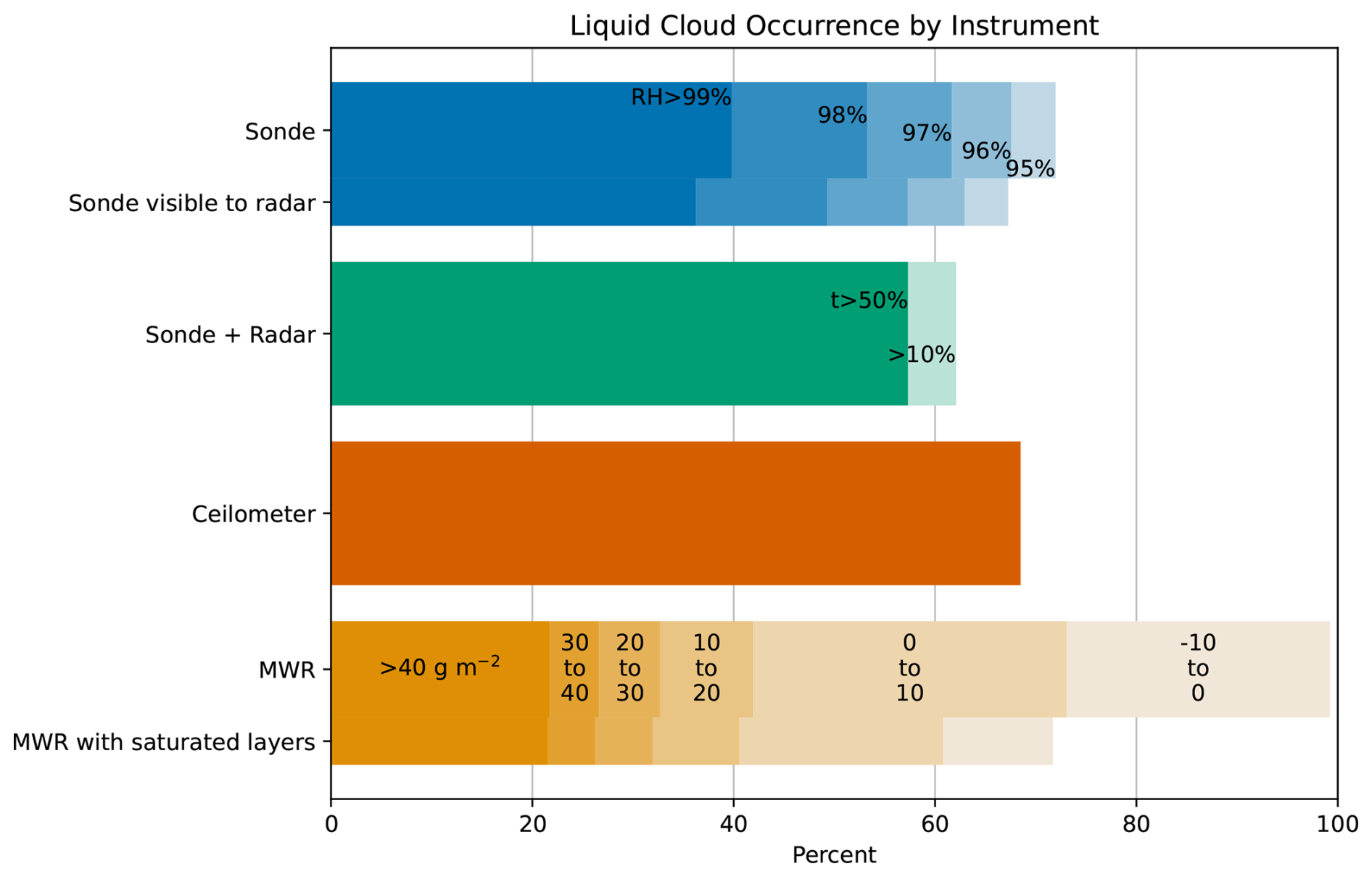
Figure 1 The percent of the time that liquid-containing clouds were detected at NSA by each instrument for November through March of 2011–2023. All percents are relative to times when no instruments (sonde, radar, ceilometer, and MWR) were missing data, for a total of 3400 data points. Shading for the “Sonde” bars corresponds to different relative humidity thresholds from 95 % (pale blue) to 99 % (dark blue), while “Sonde in radar range” shows the same but only based on sonde readings above 165 m, which is the lowest range gate detected by the cloud radar. “Sonde + Radar” is based on times when the relative humidity was above 95 % and the cloud radar detected hydrometeors in at least one of the liquid-saturated regions. Over 50 % of values at a given height had to be above the signal-to-noise threshold to be retained in the hourly average for t>50 %, and only 10 % for t>10 %. “Ceilometer” is based on times when the ceilometer detected at least one cloud base height. “MWR” is shaded according to the liquid water path in g m⁻², displayed in bins from highest (dark gold) to lowest (pale gold) values, while “MWR with saturated layers” shows the same liquid water path bins but only for times when at least one saturated layer was detected in the corresponding sonde.

Each instrument illustrates the challenge of identifying cloud liquid in a different way. For “Sonde”, there is fundamental measurement uncertainty in the relative humidity; the instrument used at NSA has a reported combined uncertainty of 3 % for relative humidity measurements (Keeler, 2025) and comparison of individual cases to the other instruments presented in Fig. 1 reveal many liquid-containing cloud layers even when relative humidity is below 100 %. Throughout the rest of this study, a threshold of 95 % will be used, which is consistent with previous studies at NSA (Silber et al., 2020, 2021). Since the cloud radar's lowest range gate is at 165 m, the “Sonde visible to radar” bar is based strictly on relative humidity at and above this height. The difference between “Sonde” and “Sonde visible to radar” indicates that about 3 % of the time the only liquid-containing clouds present are in the bottom 165 m of the atmosphere. These detections may be fogs or other very low level clouds with limited vertical extent. “Sonde + Radar” requires both a relative humidity above 95 % and detected radar reflectivity in the same height bin at the same time; the difference between this class and “Sonde” represents cases when the cloud radar did not detect hydrometeors at the same height that the soundings identified liquid-saturated cloud layers. Part of the challenge in comparing sonde to radar is in imperfect co-location; the cloud radar, ceilometer, and microwave radiometer are all at a fixed ground-based site, although with different fields of view, while the radiosonde both drifts from its release point and samples only its immediate vicinity, increasing the probability of disagreement with other instruments in a spatially heterogeneous cloud field. “Ceilometer” detects a cloud base at frequencies in line with both radiosondes and the microwave radiometer. However, the median first cloud base height derived from the ceilometer is 485 m higher than that derived from radiosondes (Fig. A1b), so the two instruments are not necessarily detecting the same liquid-containing cloud layers at a given time. Since the ceilometer is an optical instrument, optically thick ice clouds are likely to contaminate some of the ceilometer cloud base height detections, contributing to this study's reliance on other instruments for liquid-containing cloud detection throughout the rest of this analysis. Finally, the microwave radiometer “MWR” reports a best-estimate liquid water path that is displayed in bins of 10 g m⁻² from −10 up to 40 plus one bin for all values higher than that. Setting any particular threshold to identify a true positive liquid water path is tricky; we estimate the effective uncertainty to be around 10 g m⁻² (Appendix A1), but comparison to saturated layers identified by the radiosondes (“MWR with saturated layers”) indicates that most of the measurements in the 0–10 g m⁻² range correspond to identifiable cloud liquid. Liquid water path features heavily in this study, as it is one of the main determining factors of the surface radiative impact of clouds, so the analysis that follows will use a combination of broad liquid water path bins and correspondence with positive detections by other instruments to select for significant liquid water path values.

Whichever instrument or detection threshold is used, it is clear from Fig. 1 that liquid-containing clouds are extremely common at the North Slope of Alaska in winter. However, the longwave radiative impact of those clouds can vary widely depending on their opacity (closely related to the liquid water path) and temperature. Downwelling longwave radiation from liquid-containing clouds in Arctic winter increases dramatically with liquid water path up to about 30 or 40 g m⁻² (Fig. A2). Beyond that, the cloud emissivity approaches unity, i.e. the cloud becomes opaque, such that increasing cloud liquid does not further increase the downwelling longwave irradiance. Liquid water paths below about 40 g m⁻² are therefore of particular interest, as they represent the range within which relatively small variations in liquid water path or other cloud properties produce large changes in surface radiative impact. Two questions naturally arise: what conditions are favorable for liquid-containing clouds, and what factors control how much liquid those clouds have?

3.2 Cloud base controls on LWP

Previous work has shown liquid water path in the Arctic to depend on cloud base temperature, albeit in summer (Lin et al., 2003) or in idealized models (Zhang et al., 2020). The adiabatic liquid water path framework also predicts dependence on cloud base temperature, so we next investigate this relationship. Given the longwave radiative dependencies just discussed, we focus on three categories of liquid water path: Indeterminate cases, where LWP is less than 10 g m⁻² and therefore within the effective uncertainty range of zero for the radiometer but could contain some thin clouds; Semi-transparent cases, where LWP is between 10 and 40 g m⁻² and the surface radiative effect is particularly sensitive to changes in liquid content; and Opaque cases, where LWP is above 40 g m⁻² and the longwave radiative effect of the cloud is saturated.

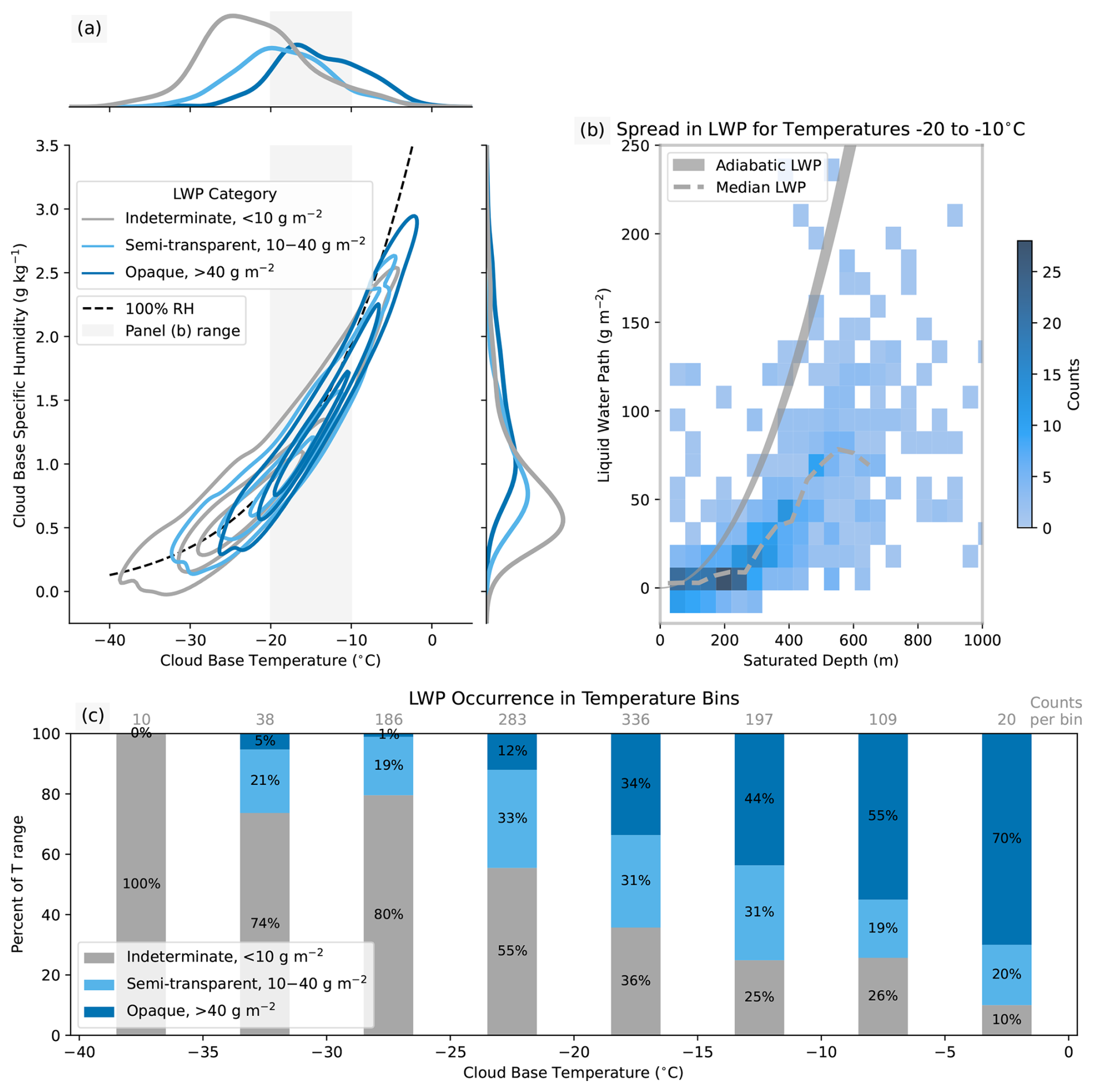
Figure 2 The relationship between liquid water path from the microwave radiometer and cloud-base conditions from radiosonde soundings for single-layer liquid-containing clouds. A joint PDF (a) shows cloud base temperature versus cloud base specific humidity at times with only one liquid-saturated cloud layer. Contours are drawn at 0.1, 0.4, and 0.7 iso-proportions of density, i.e. 0.1 means 10 % of the probability mass lies outside that contour, for three different liquid water path ranges separated at 10 and 40 g m⁻². The dashed line corresponds to a relative humidity of 100 %. The border plots are marginal distributions for temperature (top) and for specific humidity (right) as kernel density plots. The grey shaded box in (a) highlights the temperature range shown in (b), which compares liquid water path to saturated depth between −20 and −10 °C. The grey shaded curve corresponds to the predicted adiabatic liquid water path (Eq. 1) as a function of saturated depth spanning the same temperature range and using the median pressure at saturated layer base. Panel (c) shows the same data as (a) but with each LWP category as a percentage of the cloud base temperature bin, with the total number of cases per bin printed above.

The relationship between cloud base temperature, specific humidity, and liquid water path is shown in Fig. 2. Since the cloud base conditions are tied to a single cloud layer whereas liquid water path is a column-aggregated measurement, data in the figure is restricted specifically to cases with only one liquid-saturated layer as identified by the sounding. While cases were not selected for any particular temperature, it happens that nearly all single-layer cloud bases in the months and years analyzed fall in the supercooled liquid temperature range between about −38 and 0 °C. Each observation shown has both a defined liquid water path from the microwave radiometer and a saturated layer detection from the sounding, so at least two instruments agree that liquid water is present.

As they must, observations of cloud base conditions in panel (b) lie close to the black dashed Clausius-Clapeyron relationship between temperature and specific humidity at 100 % saturation, indicating that either variable could reasonably be used to describe the cloud base state. In the broadest sense, liquid water path is a function of cloud base temperature. Panel (c), showing the breakdown into LWP categories by cloud base temperature, demonstrates that the coldest cases below −25 °C have under 10 g m⁻² of liquid water more than two-thirds of the time, while the warmest cases above −5 °C are almost always opaque, although there are few enough observations at those extremes that these data may not be representative. A steady increase in the median liquid water path with cloud base temperature is also evident in Fig. A3, which further shows that each liquid water path distribution between −30 and −10 °C in bins of 5 °C is significantly different from every other in that temperature range at the 95 % level using a Kolmogorov-Smirnov test (hereafter the standard for “significantly different”). However, at intermediate temperatures between −25 and −5 °C, any of the three liquid water path categories is possible. To be specific, 73 % of all observations occur at temperatures with over a 10 % occurrence of all three liquid water path categories. The semi-transparent case, with liquid water paths between 10 and 40 g m⁻², is particularly insensitive to temperature, occurring in roughly 20 % to 30 % of cases at every temperature between −35 and 0 °C. The variability in liquid water path is high enough in this temperature range to preserve both very low and very high liquid amounts at any temperature. If these point measurements are indeed sampling stages in the cloud lifecycle, that could help explain the large range in liquid water path at any given temperature.

To determine whether cloud depth can explain the variation in liquid water path at a given cloud base temperature, Fig. 2b shows the relationship between liquid water path and saturated depth for cloud base temperatures between −20 and −10 °C, highlighted with a grey box in panel (a). Liquid water path scales with saturated depth reasonably well, but the spread is large, particularly in the semi-transparent regime, with saturated depths from 200 to nearly 800 m producing the same liquid water path. Liquid water path is also significantly sub-adiabatic under these conditions, with values falling well below the shaded region that indicates the predicted liquid water path for a given cloud base temperature and saturated depth. While the co-existence of ice can produce a sub-adiabatic liquid water path, more cloud ice within the liquid-containing layer does not generally result in a greater departure from adiabaticity for these clouds (Fig. A4).

3.3 Meteorological controls on LWP

Instantaneous cloud base conditions and total cloud depth are clearly not enough to explain liquid water path alone. But clouds do not develop in isolation. Moisture, shear, inversions, turbulence, and more in the surrounding environment can interact with cloud layers and influence their properties. Atmospheric rivers have been shown to increase cloud water and cloud liquid (Liu et al., 2018; You et al., 2022), so perhaps it is the bulk moisture and temperature of the air mass rather than the conditions just at cloud level that shape the liquid water path. The covariance between precipitable water vapor (PWV), which is the total amount of water vapor in a vertical column, and cloud liquid and ice is considered next.

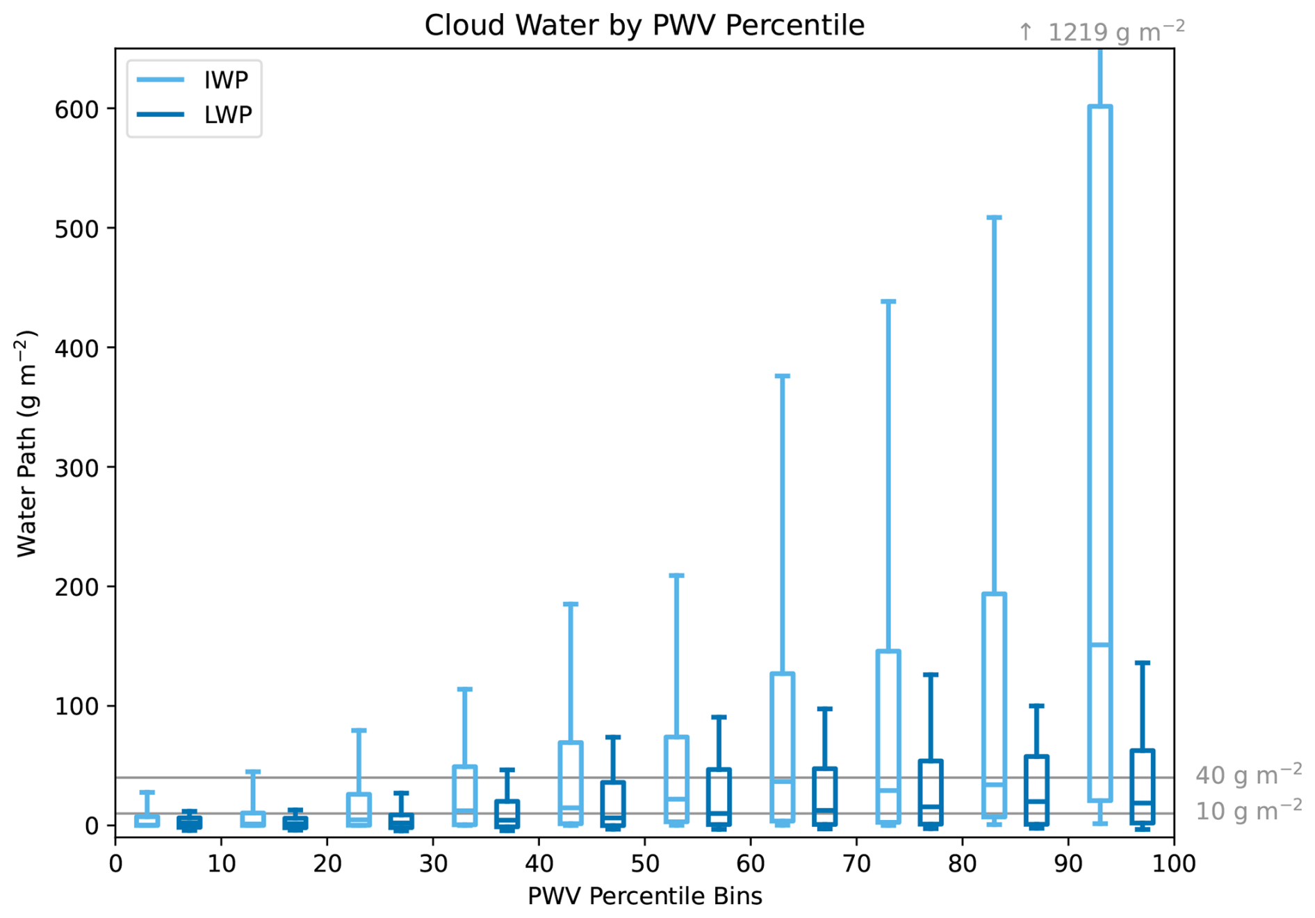
Figure 3 Box-and-whisker plots for ice (light blue) and liquid (dark blue) water path as a function of precipitable water vapor (PWV) percentile range, where PWV is the microwave radiometer best estimate. Ice water paths are derived from cloud radar reflectivities while LWP and PWV are measured by microwave radiometer. Whiskers extend to the 10th and 90th percentiles of cloud water path. Each percentile bin has 371 samples each of liquid and ice water path. Grey horizontal lines bracketing the semi-transparent regime for liquid at 10 and 40 g m⁻² are included for reference, as well as the above-axis whisker height for ice water path in the 90–100 percentile range.

Figure 3 shows the liquid and ice water paths as a function of precipitable water vapor percentile, now utilizing the full data set rather than just single-layer liquid cases. It is immediately apparent that both cloud liquid and cloud ice increase with PWV. The largest difference is in the occurrence of high cloud water values, with the 75th percentile (top of each box) increasing from 7 to 602 g m⁻² for ice and 6 to 63 g m⁻² for liquid between the lowest and highest PWV bins. Ice is more sensitive in the middle of the distribution as well, with the median ice water path increasing from 0 to 151 g m⁻² over the same range while liquid water path goes from 2 to just 19 g m⁻². However, the increase in liquid water path stagnates in the highest PWV bins. While ice water path increases dramatically in the 90th percentile of PWV, none of the liquid water path distributions above the 60th percentile are significantly different from each other (Fig. A5). A muted response of liquid water path to high atmospheric water vapor has also been observed at Summit, Greenland (Wedum et al., 2026). The differing responses of liquid and ice at the highest PWV values indicates that most of the excess available moisture is going into ice rather than liquid. But high PWV does not ensure high cloud water, and low PWV does not prohibit it. When PWV is above the 90th percentile, a quarter of all cases still have a total condensed water path less than 65 g m⁻² (Fig. A6b). Conversely, radiatively opaque liquid-containing clouds still occur at least 10 % of the time for PWV values in the 30th percentile, so they clearly do not require particularly high PWV to form.

Temperature and moisture certainly play some role in setting liquid water path. But it is equally true that virtually any commonly occurring temperature or moisture, be it at cloud level or for the air mass as a whole, can support virtually any liquid water path. Next, we extend to information about wind direction as a proxy for air mass age and coupled temperature-moisture conditions.

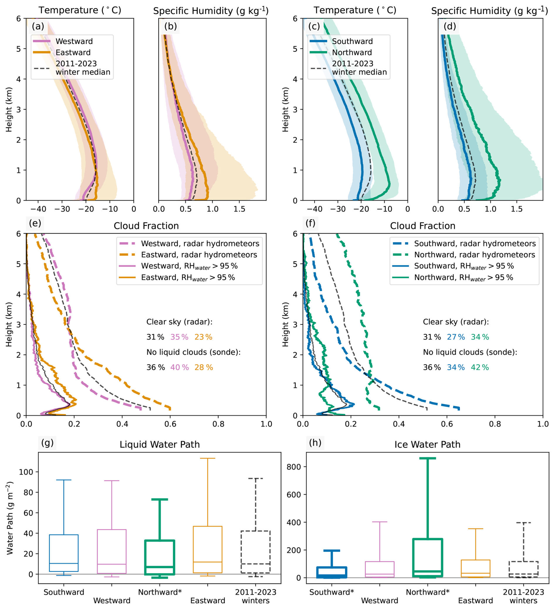
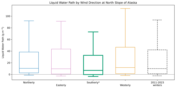
Figure 4 Panels compare conditions during westward (45 to 135°; in pink) and eastward (225 to 315°; in orange) winds (panels a, b, e, g) and between southward (315 to 45°; in blue) and northward (135 to 225°; in green) winds (panels c, d, f, h) at 500 m at North Slope of Alaska as detected by radiosondes: temperature (a, c) and specific humidity (b, d) profiles; vertical profiles of cloud fraction from the radar (e, f; dotted lines) and liquid cloud fraction from soundings (solid lines); box-and-whisker plots of liquid (g) and ice (h) water path, excluding radar-detected clear sky cases. Shaded regions correspond to the 25th to 75th percentile range (a-d). Saturated regions (e, f) are defined as RH > 95 % in soundings. Box-and-whisker plots (g, h) are bolded and labeled with an asterisk if the distribution is significantly different from the 2011–2023 winter distribution, and whiskers extend to the 10th and 90th percentiles. Black dashed lines in all panels are the median over all 2011–2023 winters, while the black solid line in (e, f) is the 2011–2023 winter median for the RH > 95 % condition.

Wind direction at NSA serves as a simple first step towards classifying by meteorological regimes. The distribution of wind direction at 500 m, near the median liquid-containing cloud base height, is bimodal, with one peak for westward winds and another for eastward winds (Fig. A7). Defining each wind category as a 90° slice centered on 0 (Southward), 90 (Westward), 180 (Northward), or 270° (Eastward), Fig. 4 compares these four regimes across multiple observation metrics. Wind direction regimes carry marked differences in both meteorology and cloud properties. Eastward and northward conditions are both warmer and moister than the winter median over at least the bottom kilometer, where most liquid-containing clouds are located according to panels (c) and (d). This is true also for the subset of times that already contain liquid-containing clouds (Fig. A8). Westward winds have a lower cloud fraction (panels e and f, where cloud fraction is all radar-detected hydrometeors) near the surface, being generally colder and drier there, but so do northward winds despite being both warm and moist. However, despite these substantial differences in temperature, moisture, cloud fraction, and even liquid cloud fraction, the wind-dependent behavior of cloud condensed water paths is unique and even appears inconsistent with other properties. Liquid water path distributions for southward, westward, and eastward winds are not significantly different from the overall winter distribution. Despite being the warmest and moistest wind direction, northward winds are associated with the statistically lowest liquid water path distribution. Additionally, these northward winds have much larger ice water paths while southward winds, which are much colder, have the lowest ice water paths, both of which are significantly different from the overall winter distribution. Thus, liquid water path is not strongly controlled by the many factors that vary with wind direction and do lead to differences in other cloud and atmospheric properties.

3.4 The large-scale circulation perspective

To better capture aspects of the regional air mass history, we turn to self-organizing maps (SOM) to classify the 6-hourly sea level pressure anomalies around the North Slope into a series of 12 nodes. The sea level pressure anomalies for each SOM node and corresponding wind directions at 500 m at NSA are shown in Fig. 5, while Fig. 6 shows the associated temperature and moisture anomalies. Each panel corresponds to a single SOM node, displayed in the same location in both figures, with the corresponding wind direction, temperature, or moisture taken from all soundings at times when the large-scale circulation was identified to be within that node. The SOM nodes meaningfully capture significant variations in wind direction, temperature, and moisture at NSA, providing a useful classification of meteorological regimes. Variations in sea level pressure anomaly are primarily expressed through the strength and positioning of the Beaufort High-Aleutian Low dipole, which is a characteristic feature of the wintertime circulation in this region. There is fairly close correspondence between large-scale circulation and wind direction at NSA, with the primary wind direction rotating counter-clockwise about the wind rose as one proceeds clockwise around the SOM. A strong Beaufort high in the lower left corner corresponds to westward winds (Fig. 5i, j, k), with dry air coming out of the Central Arctic and northern Canada that produces a cold anomaly near the surface but a warm anomaly aloft (Fig. 6i, j, k). The SOM transitions to south-westward winds in the upper left corner (a, b), bringing uniformly cold and dry air masses from the Central Arctic. In the upper right corner (c, d, g) are weaker pressure anomalies with assorted but mostly eastward winds, bringing air out of Russia and the Central Arctic. The lower right corner (h, l) features air masses arriving on northward winds out of the North Pacific with surface-amplified warm and moist anomalies. As is characteristic of a SOM analysis, the most similar sea level pressure patterns are nearest each other while the most different are furthest apart. The smooth variation in corresponding temperature and moisture anomalies across the SOM space indicates that they tend to vary in consistent ways with the large-scale circulation.

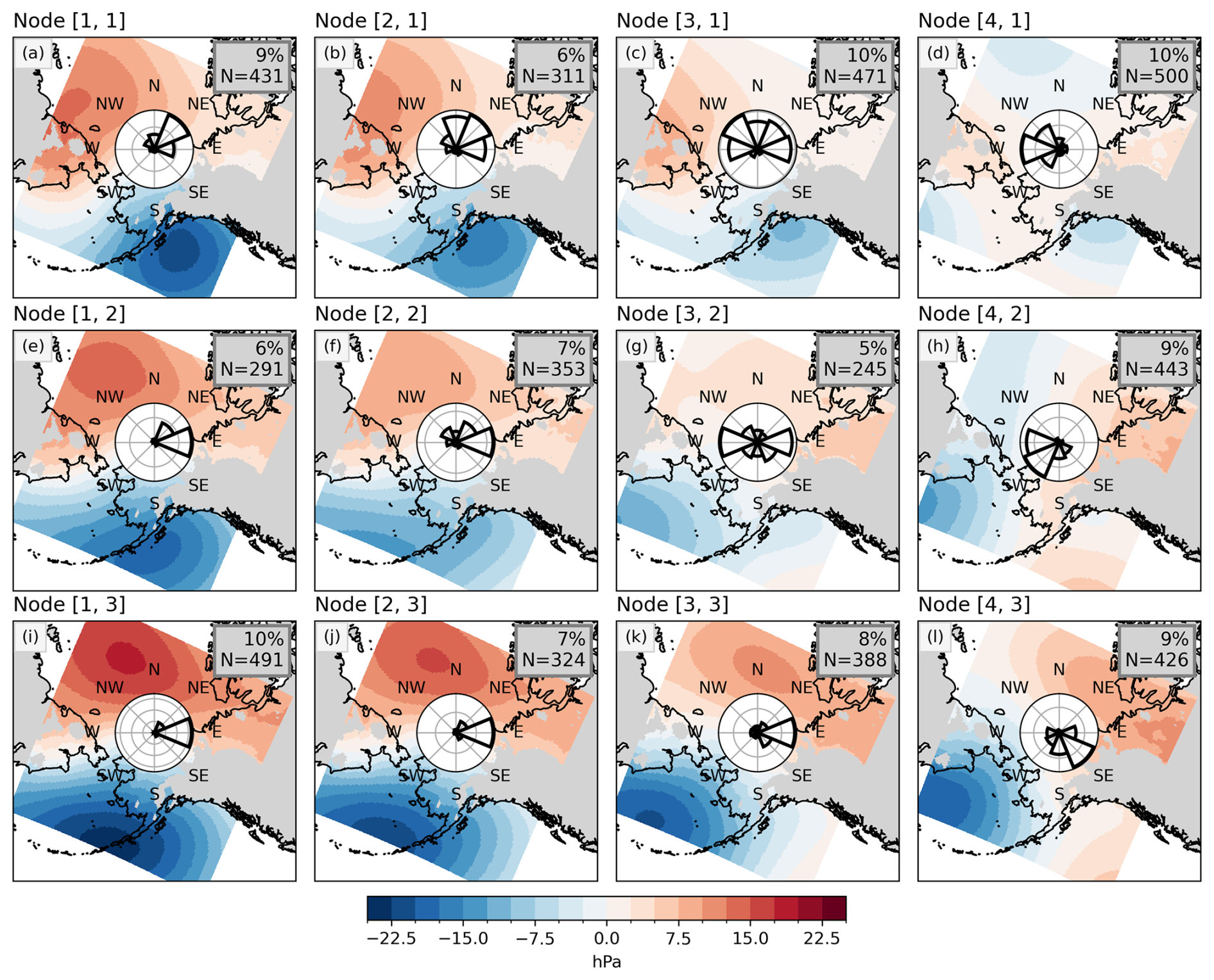
Figure 5 Sea level pressure anomalies based on ERA5 output of each self-organizing map (SOM) node are shown in shaded contours while a wind rose gives the distribution of 500 m wind direction according to radiosondes at NSA during each node. The frequency of each node from 2011–2023 is given in the upper right-hand corner.

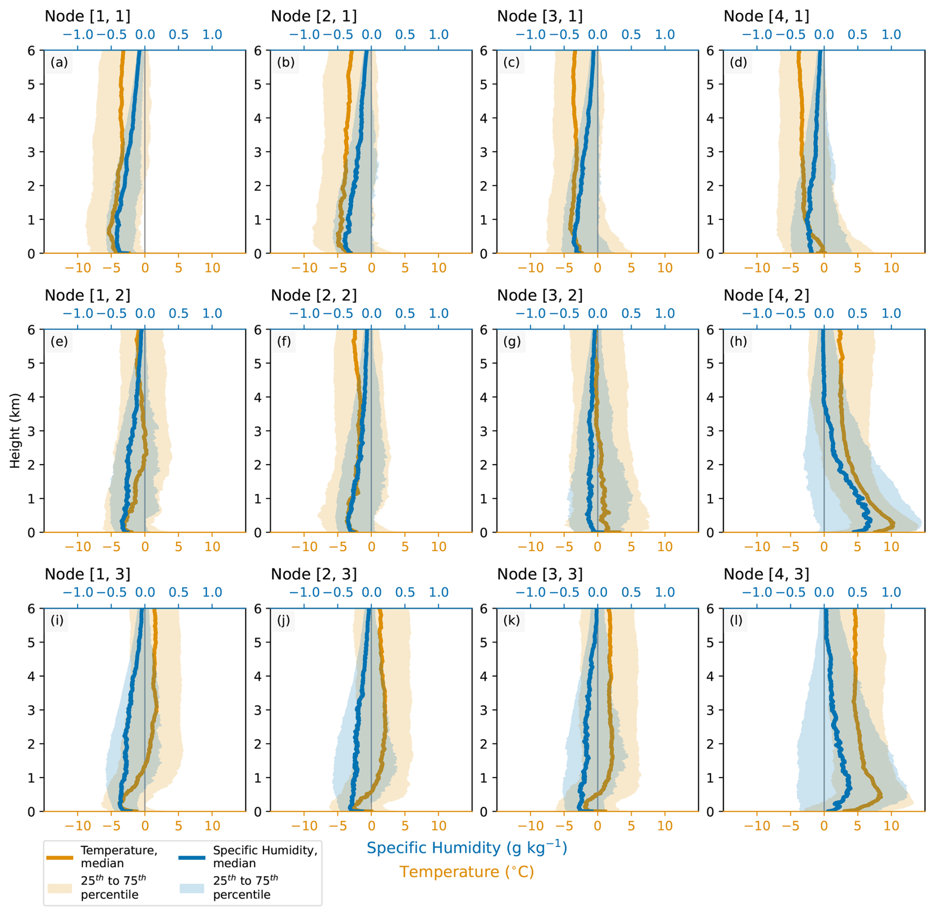
Figure 6 Vertical profiles of the difference between conditions during each node and the 2011–2023 extended winter mean for temperature (gold) and specific humidity (blue) from radiosondes. For each node, the median (solid line) and 25th to 75th percentile (shaded region) of anomalies from the winter mean are represented. The lower x-axis gives temperature in degrees Celsius while the upper x-axis shows specific humidity in g kg⁻¹; both axes scales are the same for all panels. The node label is given above each plot, and the positions within the grid are the same as in Fig. 5.

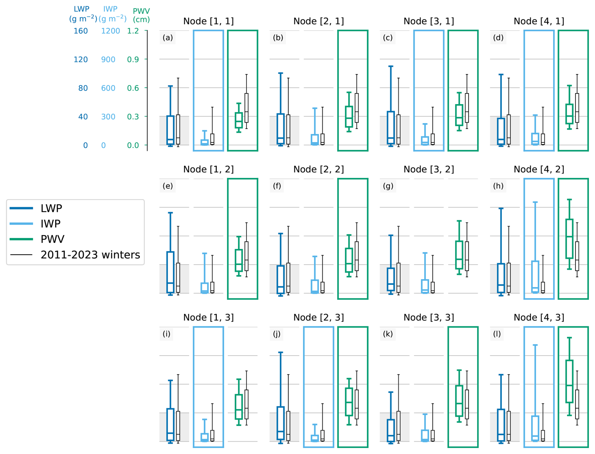
Figure 7 Box-and-whisker plots of liquid water path (dark blue) on the left, ice water path (light blue) in the middle, and precipitable water vapor (green) on the right during each SOM node. Clear-sky cases are excluded from all distributions. Whiskers extend to the 10th and 90th percentiles. The black plots are the distribution over all 2011–2023 winters and therefore the same for all nodes. If the distribution for a given node is significantly different from that of all 2011–2023 winters, that plot is outlined in the corresponding color.

While total atmospheric moisture and cloud ice also tend to vary significantly with the large-scale circulation, liquid water path does not. Figure 7 shows the liquid water path, ice water path, and precipitable water vapor distributions for each SOM node compared to their distributions over all 2011–2023 winters. As expected, most nodes have a precipitable water vapor that is significantly different from 2011–2023 winters as a whole, marked by a green outline, demonstrating that total atmospheric moisture is highly constrained by the large-scale circulation. Additionally, just over half of the nodes have significant differences in ice water path, marked by a light blue outline. To the extent that SOM nodes represent meteorological regimes, moisture therefore varies consistently with meteorology and ice water path largely responds to those variations. However, not a single node has a liquid water path distribution that is statistically distinguishable from 2011–2023 winters as a whole. Even the warm and moist nodes in the lower right corner, which have the highest occurrence of the highest percentile bins of precipitable water vapor from Fig. 3 and notably high ice water path, show only statistically insignificant variations from the background liquid water path distribution. Adjacent nodes, which have the most similar circulation, temperature, and moisture, do not even have anomalies of the same sign with respect to typical wintertime conditions; just compare [1, 1] to [1, 2], or [3, 1] to [4, 1]. On the whole, the meteorology itself and even cloud ice water path show significant sensitivities to the large-scale circulation regime. By contrast, liquid water path is remarkably insensitive to large-scale circulation, with similar circulation regimes producing different and, ultimately, insignificant liquid water path anomalies.

4 Discussion

Using over ten years of observations from multiple ground-based instruments coordinated with radiosondes at NSA in winter, this study probed relationships between meteorological conditions and cloud phase with a particular focus on cloud liquid water path. Beginning with simple assumptions about how cloud base conditions and air mass history might influence cloud phase, we sought to understand the extent to which variations in these conditions could explain the overall distribution of cloud liquid and ice water path. Surprisingly, we found that while ice water path scales with bulk atmospheric moisture, liquid water path is remarkably insensitive to meteorology and large-scale circulation, raising questions about the fundamental processes governing liquid-containing cloud layers, interactions between cloud ice and cloud liquid, and how the coupled Arctic system will respond to a warming climate.

The results presented throughout this study suggest two key conclusions that begin to shape the path for further investigation. First, liquid water path is only weakly dependent on cloud base temperature in the temperature ranges most relevant to wintertime Arctic mixed-phase clouds. This can be seen directly for cases with a single liquid-containing layer shown in Fig. 2. While there is an increase in median liquid water path from −25 to −5 °C, which accounts for about three-quarters of all wintertime liquid-containing clouds at NSA, variability is high enough that all temperatures in this range allow for any liquid water path from optically thin to optically thick. Second, both low and high liquid water path frequencies are largely insensitive to changes in meteorological regime. The liquid water path distribution is statistically indistinguishable across meteorological regimes as defined by either 500 m wind direction (Fig. 4) or by SOM nodes (Fig. 7). Ultimately, neither cloud base temperature nor wind direction nor large-scale circulation regime appear to be reliable predictors of liquid water path.

A more robust indicator, one with a somewhat clearer relationship with cloud liquid and cloud ice than wind direction or large-scale circulation, is precipitable water vapor. Ice water path increases monotonically with precipitable water vapor while liquid water path increases up to the 60th percentile of PWV before leveling off (Figs. 3 and A5). However, just because specific precipitable water vapor ranges have significant differences in cloud liquid water path does not appear to mean that changes in precipitable water vapor distribution lead to changes in liquid water path distribution. As evidence, consider cloud and atmospheric water vapor distributions distinguished by SOM node in Fig. 7, where many nodes have a precipitable water vapor or ice water path distribution significantly different from the typical wintertime conditions from 2011 to 2023 but none has a significantly different liquid water path distribution. Two factors appear to be at work here. On the one hand, all but the very highest precipitable water vapor bins still have less than 20 g m⁻² of either ice or liquid in the majority of cases (Fig. 3), so high water vapor is not a guarantee of high condensed water path. On the other hand, while some circulation regimes are more likely to bring high precipitable water vapor, they do not exclusively do so. Just under half of all cases for the two moistest SOM nodes have precipitable water vapor below the 75th percentile of 2011–2023 wintertime conditions for PWV. Taken together, the relatively modest increase in liquid water path with PWV (Fig. 3) plus the wide range of PWV for any given SOM node (Fig. 7) means that even the circulation regimes favorable to high precipitable water vapor do not necessarily lead to high liquid water path.

Throughout these results, the Clausius-Clapeyron relationship emerges as a strong constraint on cloud liquid water path in a way that is perhaps counter-intuitive. First, as long as an air mass is on or near the saturation curve, any cooling supports cloud formation. The exponential relationship between temperature and moisture at saturation requires more cooling with a colder initial temperature at the same relative humidity, but saturation is always accessible, as evidenced by the consistency of the liquid water path distribution even during colder, drier conditions such as southward winds (Fig. 4) and SOM nodes [1, 1] and [2, 1] (Figs. 6 and 7). Second, warm and moist air masses are not necessarily any closer to saturation than cold and dry ones as long as moisture is measured in absolute terms. If the excess moisture is not sufficient to compensate for the excess temperature, then warmer and moister conditions will not necessarily bring more cloud liquid, as seen in the lack of response of the liquid water path distribution to meteorological conditions with high moisture in Figs. 3, 4, and 7.

We next propose a collection of key processes that could explain the unexpected insensitivity of cloud liquid water to meteorology and large-scale circulation observed in this study. Preliminary support for some processes can be found in the figures above, and particularly in the Appendices, but all will require further analysis to either validate or discard.

• Hypothesis 1: Continuous radiative cooling and a lack of dissipative mechanisms allow the liquid-containing clouds that frequently form to persist for long periods of time, as suggested by Herman and Goody (1976). The prevalence of clouds with low liquid water path may simply be a consequence of a lack of dissipative mechanisms in a highly stratified environment and continuous air mass cooling. Many of the dissipative mechanisms active at lower latitudes are much weaker in the Arctic in winter. Cloud-top entrainment can actually work to maintain rather than dissipate cloud layers, as humidity inversions are common in the Arctic and cause entrainment to bring in moister rather than drier air (Solomon et al., 2011). There are fewer INPs than at lower latitudes, decreasing the efficiency of ice processes. Weak surface fluxes and strong boundary layer stability often decouple Arctic cloud layers from the surface, insulating them from surface turbulence and aerosols. Meanwhile, radiative cooling continuously drives air masses towards the saturation point and condensation. In this framework, typical conditions favor cloud persistence until either external forcings disrupt it or precipitation has removed sufficient moisture that further cooling is insufficient to bring the air mass to saturation. This persistence of low LWP clouds is seen in the consistency of the liquid water path distribution across all SOM nodes (Fig. 7) and the two predominant wind directions (Fig. 4), suggesting similar cloud LWP regardless of circulation regime or moisture availability.

• Hypothesis 2: Competing temperature dependencies among ice processes contribute to a flat temperature response for liquid water path at intermediate supercooled temperatures. At colder temperatures, ice nucleation is more efficient, with more INPs active as the temperature decreases (DeMott et al., 2016; Wex et al., 2019; Creamean et al., 2022; Gjelsvik et al., 2025), but water vapor is scarce, allowing for primarily low liquid water paths. At intermediate temperatures, around −12 °C, the difference between saturation vapor pressure over liquid and ice is maximized (Korolev and Isaac, 2003) and water vapor is more plentiful, producing a wide range of liquid and ice water paths. At warmer temperatures, water vapor becomes more prevalent, supporting more rapid ice growth to compete with the liquid via WBF and the seeder-feeder mechanism. Yet ice nucleation itself becomes less effective because there are relatively few warm temperature INPs (Creamean et al., 2022), while some proposed secondary ice processes might become more effective at relatively warmer temperatures (Korolev and Leisner, 2020; Field et al., 2017). Competing tendencies at all temperatures could produce the observed insensitivity of the liquid water path distribution at all but the warmest and coldest supercooled temperatures.

• Hypothesis 3: The efficiency of ice production depends on the amount and properties of cloud liquid, limiting the highest liquid water amounts. Once ice appears in a supercooled liquid-containing cloud, it efficiently converts liquid mass to ice mass via the WBF process. Additionally, there are a collection of ice production mechanisms that should, in theory, increase as liquid water path increases. In the relatively clean air of the Arctic, a cloud condensation nuclei (CCN)-limited regime implies that a higher condensed liquid mass results in larger rather than more numerous liquid droplets. Higher liquid water path therefore implies more liquid mass and more large liquid droplets, both of which can enhance ice nucleation, secondary ice production, and/or riming (Lauber et al., 2018; Korolev and Leisner, 2020). In this framework, cloud layers with a very low liquid water path, like those so commonly observed across the Arctic, would be poor ice-producers, shutting down one of the main dissipative mechanisms and allowing these clouds to form and persist relatively easily. A cloud layer with higher liquid water path, on the other hand, would also efficiently produce and grow ice that competes with the liquid and limits further liquid mass production. Indicators of such a feedback appear in this study in the response of cloud water to precipitable water vapor in the highest few percentile bins, as liquid water path levels off even as ice water path increases sharply.

• Hypothesis 4: When there is high precipitable water vapor, it often involves deep layers of enhanced moisture leading to enhanced ice production aloft that activates the seeder-feeder mechanism, limiting the expected increase in liquid water path. Above the 90th percentile of precipitable water vapor, there appears to be a tradeoff between cloud liquid and ice, with high values of one or the other but rarely both (Figure. A6c). Under these conditions, the largest water vapor anomalies are between 500 and 1500 m, which is located above the peak in liquid-containing cloud fraction at 350 m (Fig. A9). This indicates that much of the excess water vapor is above liquid-containing cloud layers and thus may instead contribute directly to enhanced ice production. The median anomaly in relative humidity for the highest PWV bin exceeds 20 % from 2 km to above 6 km, providing a considerable vertical distance through which ice can form, grow, and fall. Accordingly, we found that the total mass of ice above the highest liquid-containing layer increases with precipitable water vapor, with a particularly sharp increase for the highest PWV percentile bin (Fig. A10), supporting the stronger correspondence between ice water path and precipitable water vapor. The same relationship can be seen in northward winds, which bring enhanced moisture and cloud fraction aloft but lower liquid water path and liquid-containing cloud fraction in the bottom kilometer of the atmosphere (Fig. A7). The increase in ice mass aloft can also be shown to coincide with an increase in ice precipitation into liquid-containing layers: the fraction of all liquid-containing layers that have radar-detected hydrometeors directly above them, presumably precipitating ice, also increases from 57 % to 69 % from the 50th to the 90th percentile bin of precipitable water vapor (Fig. A11). Increased opacity of ice clouds has been shown to be more important than changes in partitioning between liquid and ice when explaining how net surface longwave radiation at NSA has changed with warming (Bertrand et al., 2025), so constraining ice production under warming and moistening conditions may be particularly important for a changing Arctic.

The result of these competing dependencies might help explain the observations from NSA, with low liquid and ice water paths under the very coldest and driest conditions, a relatively flat response to temperature as ice processes compete at intermediate temperatures, and high ice water paths that damp some of the expected increase in liquid water path under warm and moist conditions. As these hypotheses are supported by some information but not rigorously tested, more detailed analysis of, for example, the temperature dependence of ice production and co-evolution of liquid and ice within clouds is needed to investigate these claims.

5 Conclusions

Liquid water path in Arctic winter is weakly sensitive to temperature and moisture and largely insensitive to winds and large-scale circulation. This study uses over ten years of continuous observations from NSA across multiple instruments to investigate the correspondence between cloud liquid, cloud ice, and meteorological conditions. Radiosonde soundings, cloud radar, ceilometer, and microwave radiometer generally agree that liquid-containing clouds are present 60 %–70 % of the time at NSA between November and March. At cloud base temperatures between −25 and −5 °C, encapsulating about three-quarters of all wintertime liquid-containing clouds, a broad range of liquid water paths are accessible. Cloud ice responds strongly but liquid weakly to precipitable water vapor, particularly at the highest percentiles of available moisture. Meteorological regimes, whether defined by local wind direction or large-scale circulation, come with distinct temperature, moisture, and cloud ice conditions, but all produce statistically similar liquid water path distributions.

The remarkable persistence yet apparent insensitivity of wintertime liquid-containing clouds calls for new ideas and methods as well as revisiting older frameworks. We propose a collection of hypotheses consistent with the observations presented here, centered primarily around the continuous radiative cooling of air masses and the role of ice in enabling or limiting liquid mass accumulation. We encourage the community to challenge them with observational data and targeted model studies. A focus on dissipative mechanisms is warranted, and particularly on the conditions that limit them in many cases. An air mass transformation approach could begin to untangle what causes liquid water path to increase or decrease throughout the air mass lifecycle, although acquiring high-fidelity information on cloud water properties at sufficient spatial and temporal resolution for such an analysis remains a major technical challenge. An investigation into whether the relationships found in this study between temperature, moisture, circulation, and cloud ice and liquid water path hold at other Arctic locations or in models could also help gauge the universality of Arctic cloud properties and their implications for climate. Whatever the method, any answers to the many questions raised by these results would represent a significant step forward in our understanding of Arctic cloud properties, how they could be better represented in models, and how they might respond to changing meteorological conditions.

Appendix A

A1 Additional Data Processing Details

A1.1 Missing data

ARM provides a quality check field for each variable, regardless of instrument, with a value of zero if none of the tests failed and greater than zero if one or more tests failed. These tests include checks for missing values, values above or below a “valid” range, and a difference from the previous value that exceeds a threshold “valid_delta”. In addition, ARM Data Quality Reports indicate sections of data for each instrument that have been flagged Incorrect (and should not be used) or Suspect (values indicate underlying issues that must be subject to additional screening). In this analysis, we replace any data value from any instrument that is flagged as Incorrect or Suspect, or with a quality check value greater than zero, with NaN before performing any other processing such as averaging, interpolation, or resampling. Thus any “missing data” referred to in the text are values that the checks described above have replaced with NaN and therefore could be a result of either instrument downtime, verified or suspected instrument errors, or failure to pass quality checks. Hourly averages used in data processing ignore missing values except where stated otherwise; only if all returns for the hour are missing will the hourly average return NaN.

A1.2 LWP retrievals

The ARM best-estimate product for LWP uses a physical retrieval method when the appropriate inputs are available and a statistical method when they are not. The physical retrieval method utilizes the Atmospheric Environmental Research MonoRTM forward model and atmospheric conditions from soundings to iteratively solve for both LWP and PWV (Turner et al., 2007). Since this study restricts all datasets to times near radiosonde launches, the main limiting factor in running the physical retrieval method, the physical retrievals are almost always the source of LWP values in this analysis: 99.5 % of all LWP values that go into the calculation of hourly averages for this study come from the physical retrieval. Negative LWP values are still possible because the final guess for the atmospheric state from the retrieval algorithm, which must be within the uncertainty from the instruments and model of the previous guess and therefore converged, is not itself run through the forward model (Maahn et al., 2020).

A1.3 LWP uncertainty

ARM reports a 1σ uncertainty for these physical retrieval values that, for the data used in this study, ranges from 3 to 9 g m⁻² with a mean of 5.3 g m⁻² as well as the number of iterations it took the forward model to converge, which ranges from 2 to 6 iterations with a median of 3; there were no cases where the physical retrieval method failed to converge. If we assumed that all uncertainty is due to instrument noise, which is highly unlikely, the theoretical uncertainty in hourly averages of LWP would be the true uncertainty divided by the square root of the number of observations making up each average. At a sampling rate of 30 s and with a mean reported retrieval uncertainty of 5.3 g m⁻², the theoretical uncertainty due to instrument noise for hourly LWP would be $\mathrm{5.3}/\sqrt{\mathrm{120}}=\mathrm{0.5}$ g m⁻². In reality, a sensible LWP uncertainty should also account as much as possible for biases that result from correlation with environmental conditions implied by the spread of LWP during clear sky conditions when the “true” value is likely zero. Additionally, our primary purpose in this study is to compare LWP to the conditions reported by other instruments, so an uncertainty that reflects the degree of agreement with external measurements like the detection of liquid-saturated layers is desirable. To that end, a more conservative estimate of 10 g m⁻², which exceeds the 1σ spread in LWP during clear sky of 6.1 g m⁻² and corresponds to a change in co-occurrence with saturated layers detected by soundings (Fig. 1), is adopted as the detection threshold for this study.

A2 Supplemental Figures

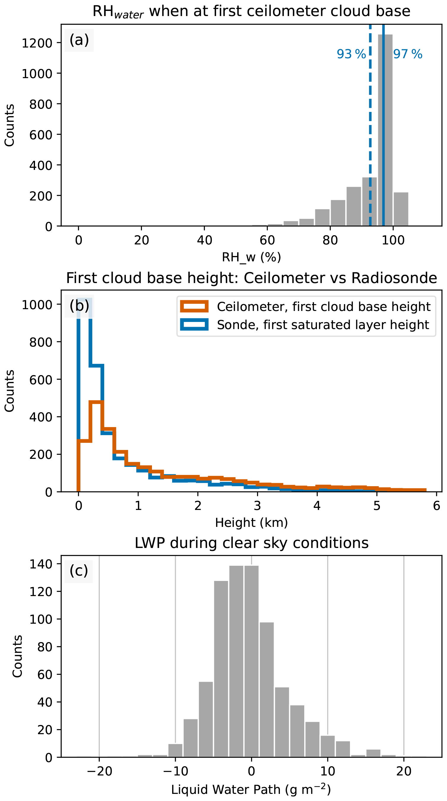
Figure A1 (a) Relative humidity with respect to liquid water from the radiosonde at the first cloud base height detected by the ceilometer. The blue dashed line and accompanying text indicate the mean of the distribution, while the blue solid line indicates the median. (b) First cloud base height from the ceilometer (rust) and the base of the first saturated layer from the radiosonde (blue). (c) Liquid water path distribution via microwave radiometer during clear sky conditions.

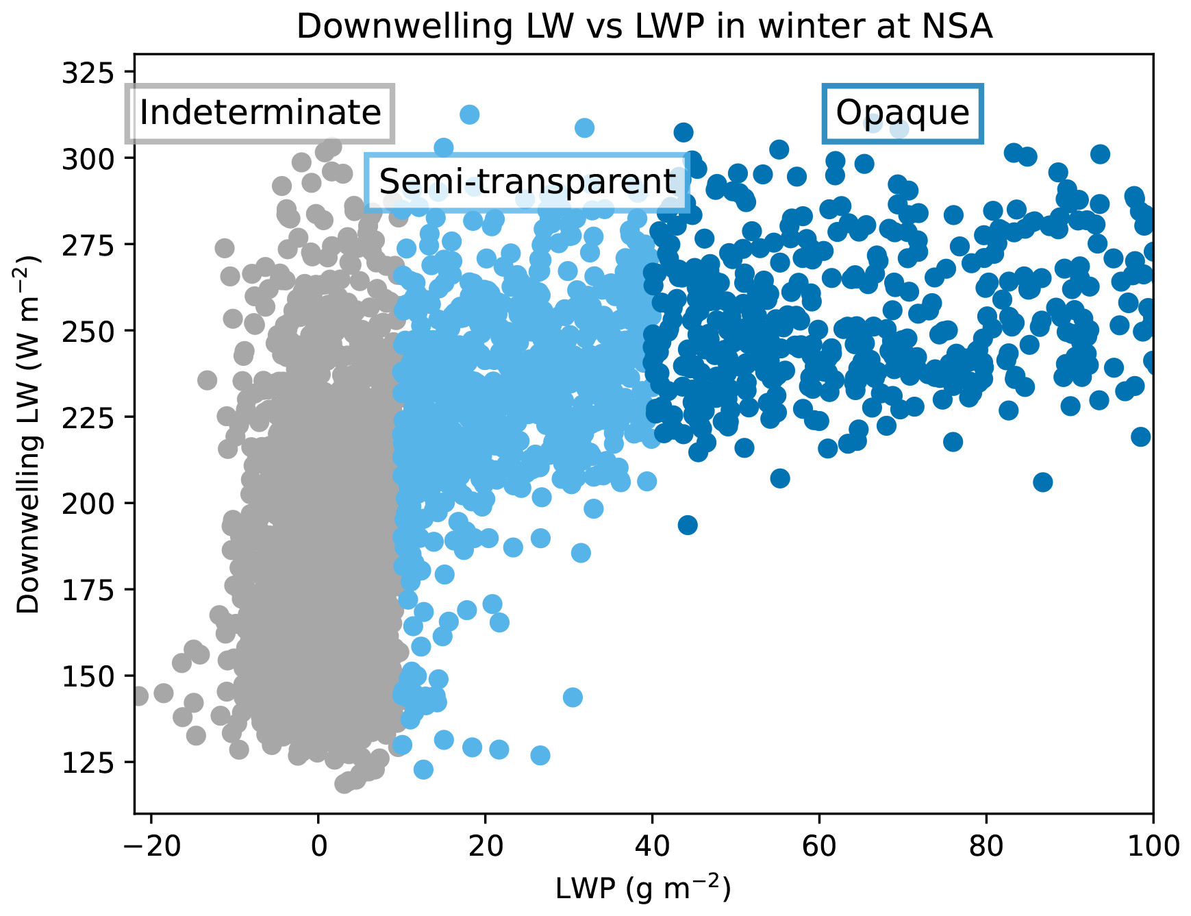
Figure A2 Downwelling longwave radiation at the surface as a function of liquid water path. Points are colored according to the three liquid water path categories defined in the paper: Indeterminate (<10 g m⁻²), Semi-transparent (10–40 g m⁻²), and Opaque (>40 g m⁻²). Downwelling longwave radiation is the downwelling longwave hemispheric irradiance reported in the qcrad1long.c2 datastream.

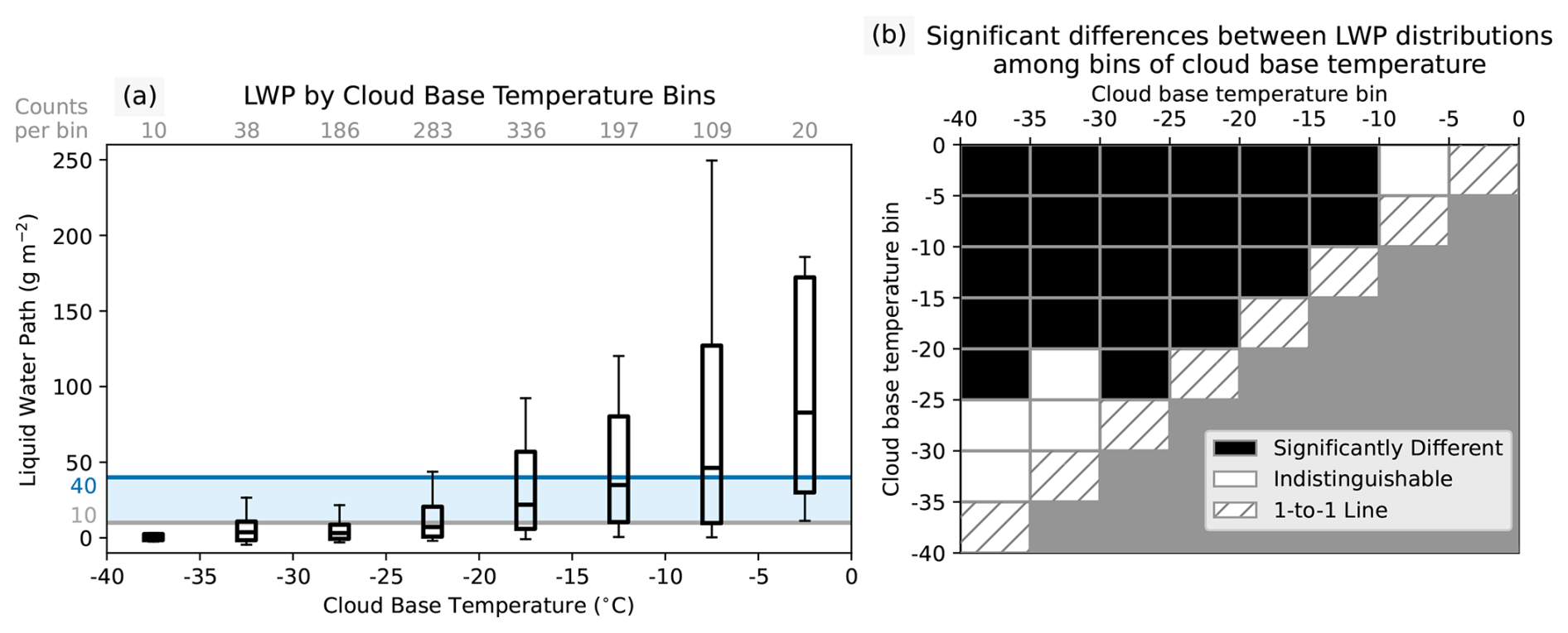
Figure A3 Liquid water path distributions as a function of cloud base temperature (a) in 5° bins for single-layer cloud cases and a significant difference matrix comparing all pairs of LWP distributions (b) at the 95 % confidence level using a Kolmogorov-Smirnov test.

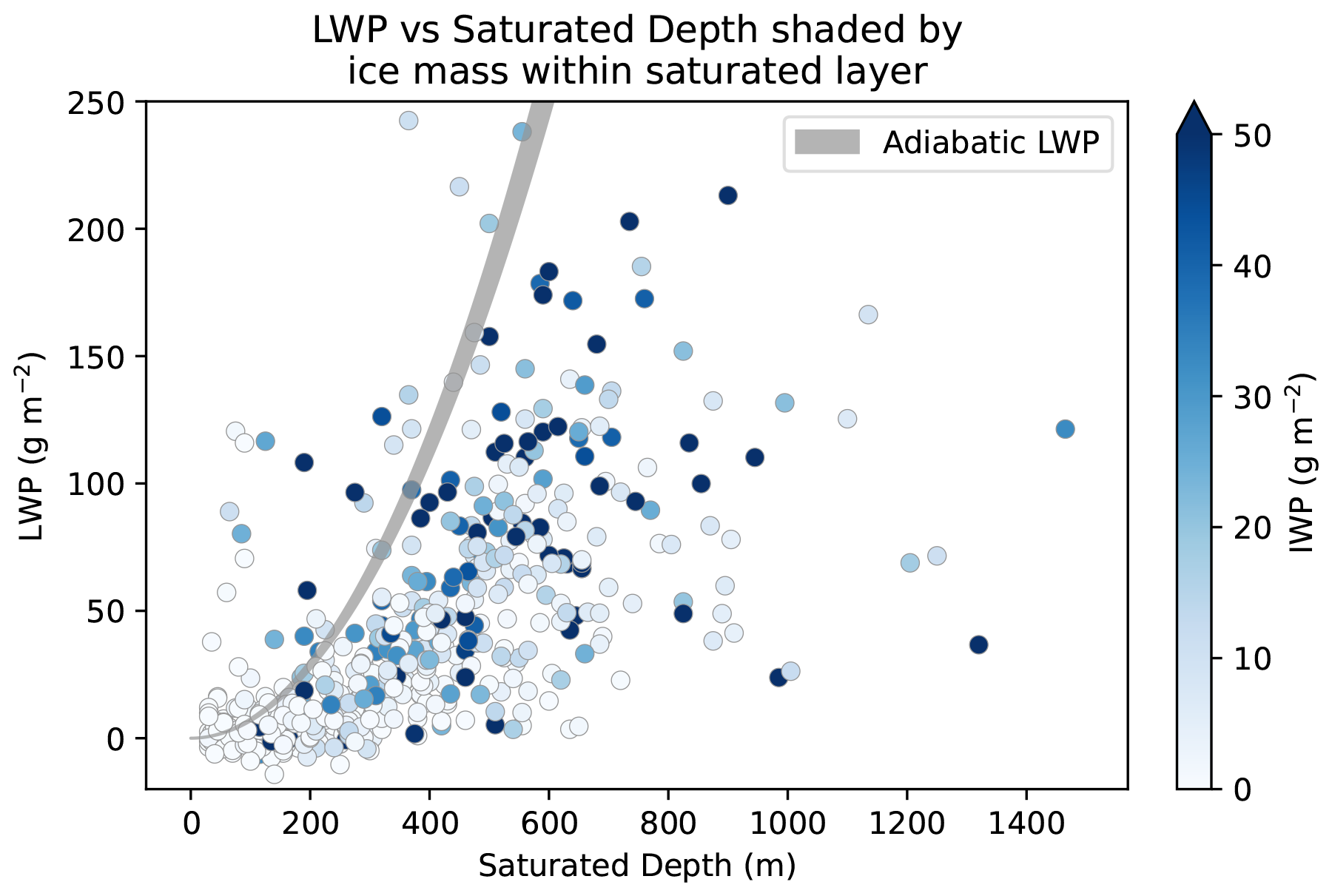
Figure A4 Liquid water path as a function of saturated depth for cases with a single saturated layer and a cloud base temperature between −20 and −10 °C, colored by the amount of ice within the saturated layer. The grey shaded region shows the adiabatic liquid water path predicted as a function of saturated depth for cloud base temperatures between −20 and −10 °C. Displays the same cases as in Fig. 2b of the main manuscript.

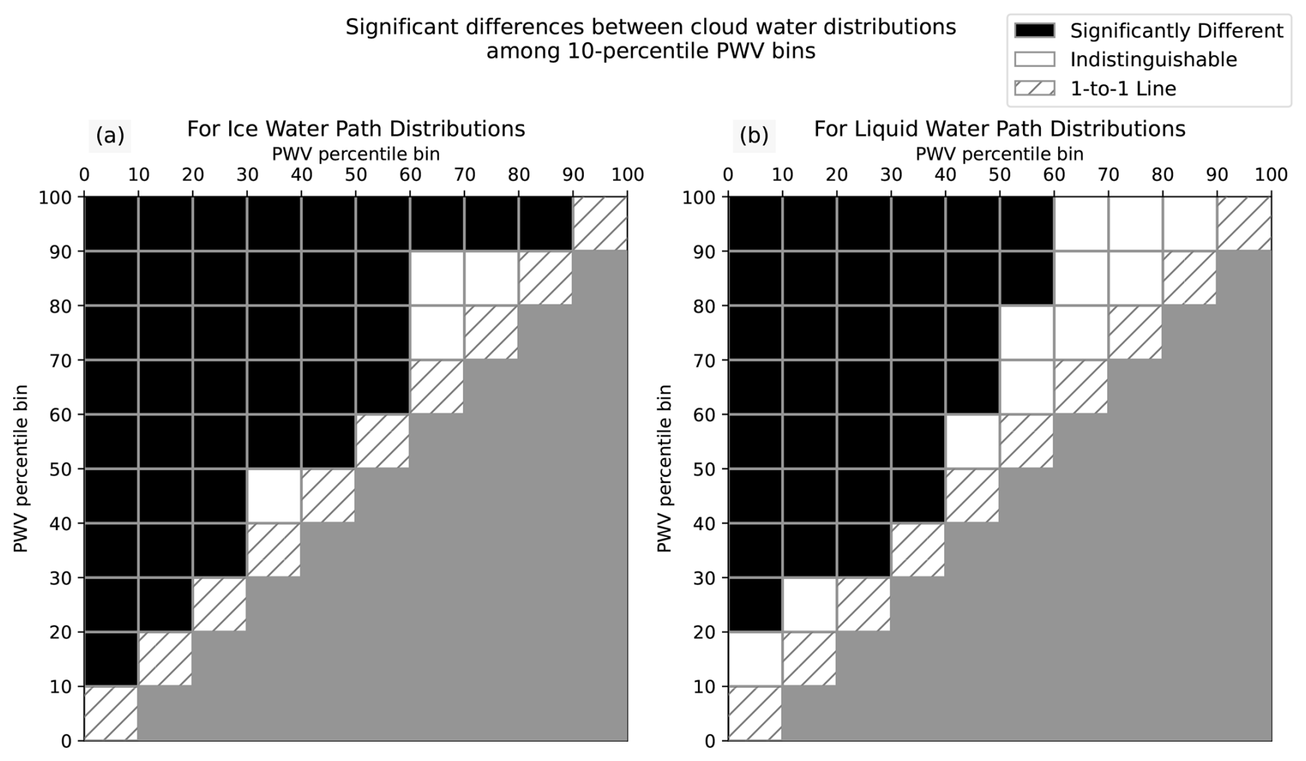
Figure A5 Significant difference flags between all pairs of ice (a) and liquid (b) water path distributions by PWV percentile from Fig. 3. Significant difference is determined at the 95 % level by a two-sample Kolmogorov-Smirnov test.

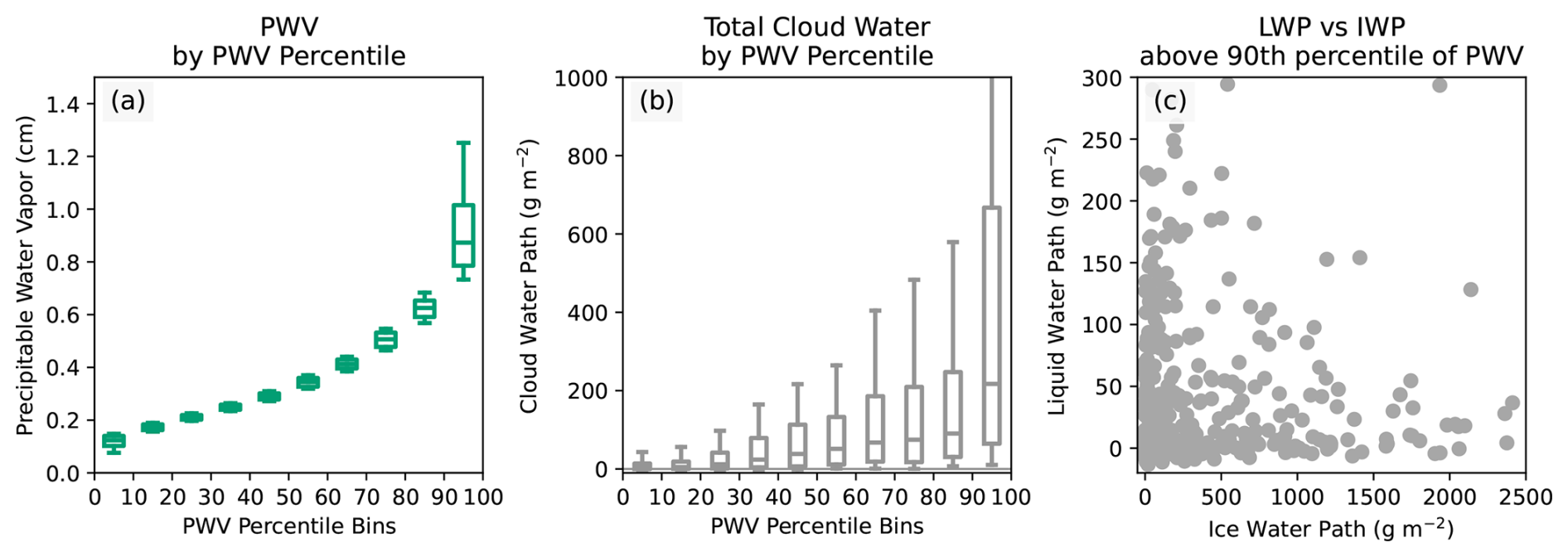
Figure A6 Box-and-whisker plots of precipitable water vapor (a) and total cloud water (ice water path plus liquid water path) (b) by precipitable water vapor percentile as well as the correspondence between liquid and ice water path for the highest precipitable water vapor bin (c). The whiskers in (a) and (b) extend to the 10th and 90th percentiles.

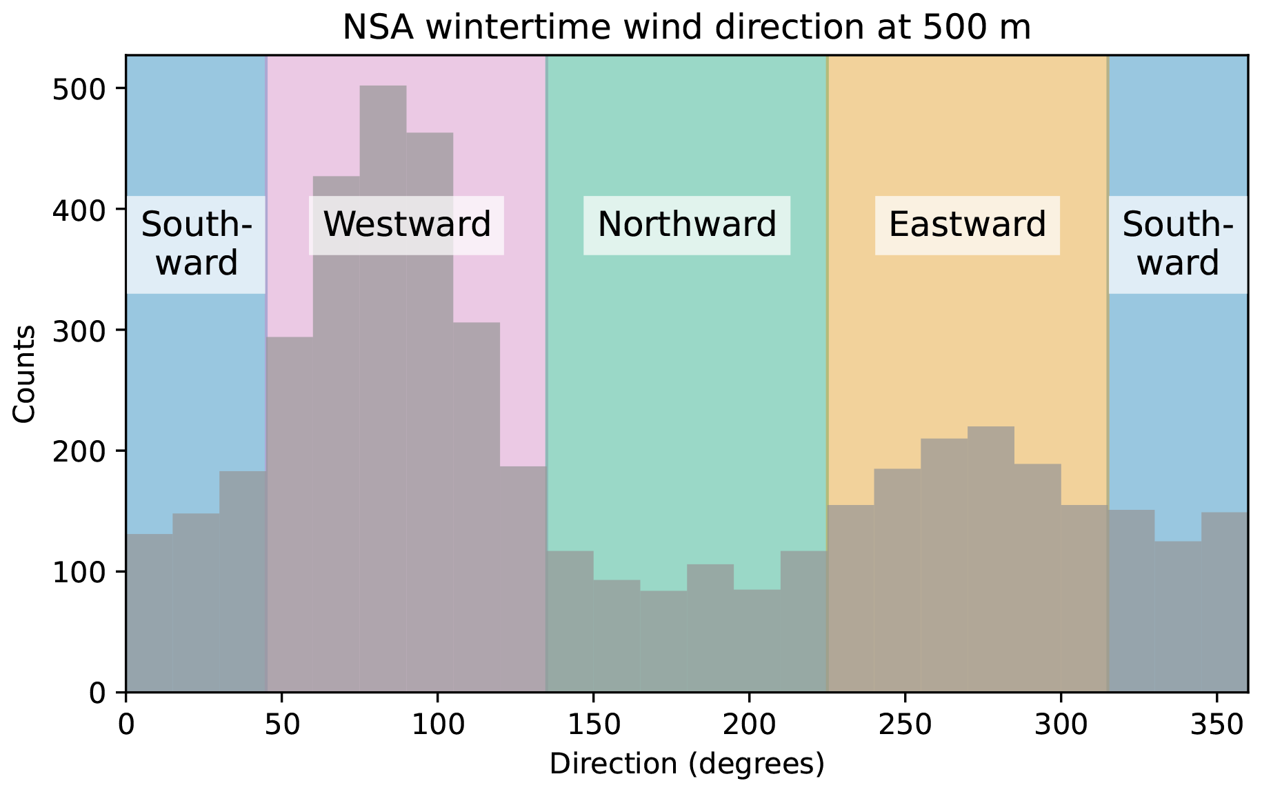
Figure A7 The distribution of 500 m wind direction at NSA, with the ranges defining southward (blue), westward (pink), northward (green), and eastward (orange) winds shaded.

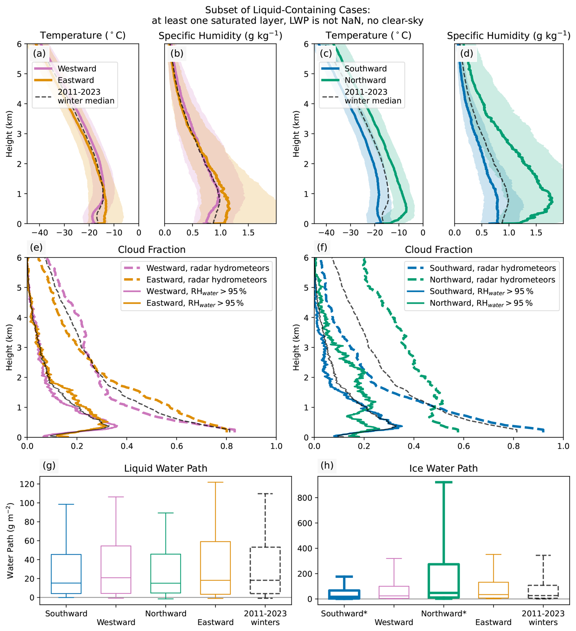
Figure A8 Same as Fig. 4 in the main manuscript, except all panels display the same subset of cases: at least one saturated layer is present, the liquid water path is defined, and the radar does not detect clear sky.

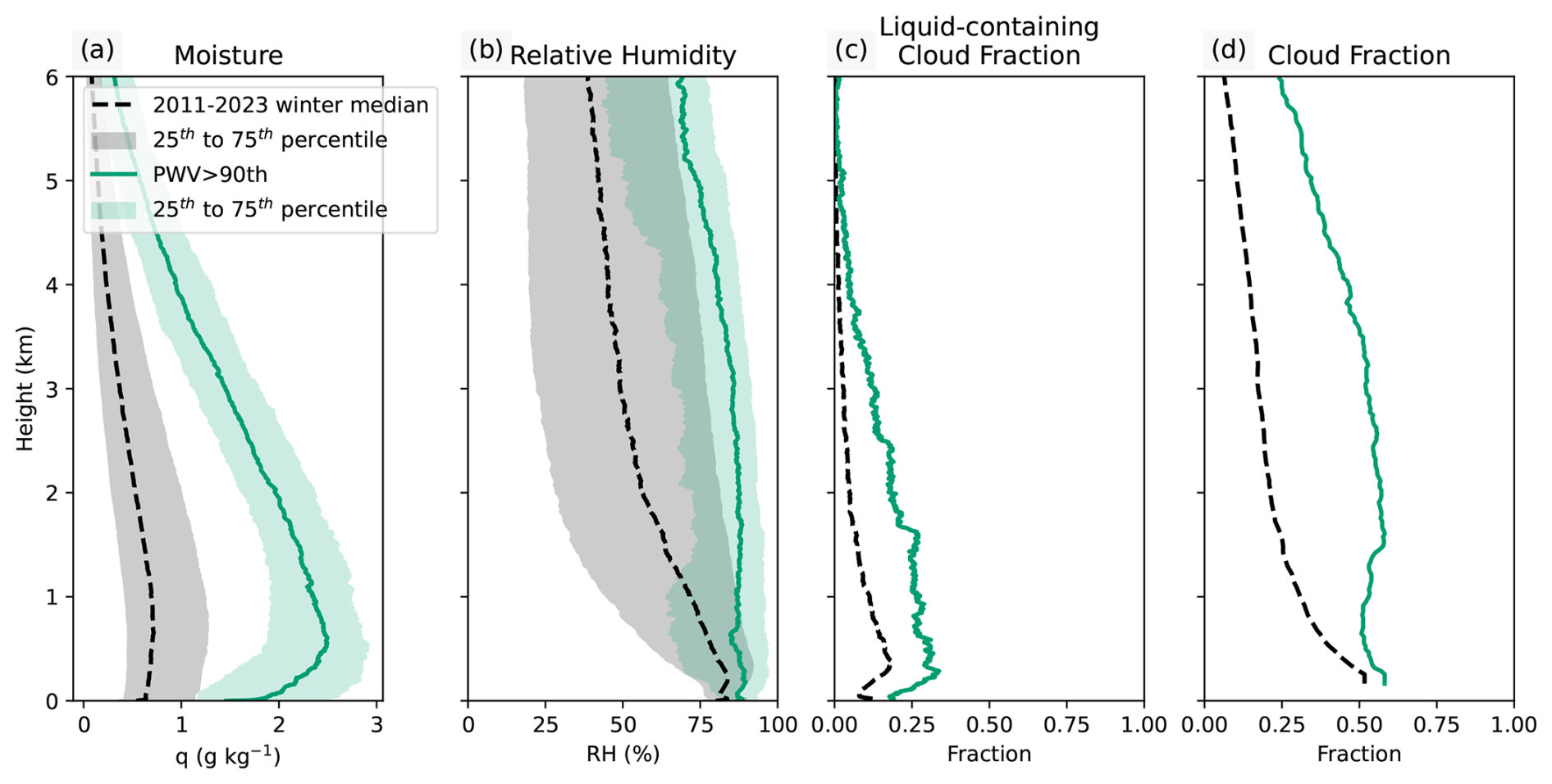
Figure A9 Comparing 2011–2023 winter median vertical profiles (in black) of specific humidity (a), relative humidity (b), saturated layer fraction (c), and cloud fraction (d) to those when PWV is above its 90th percentile (in green). Shaded regions demarcate the 25th to 75th percentile range over all cases while solid and dashed lines indicate the median.

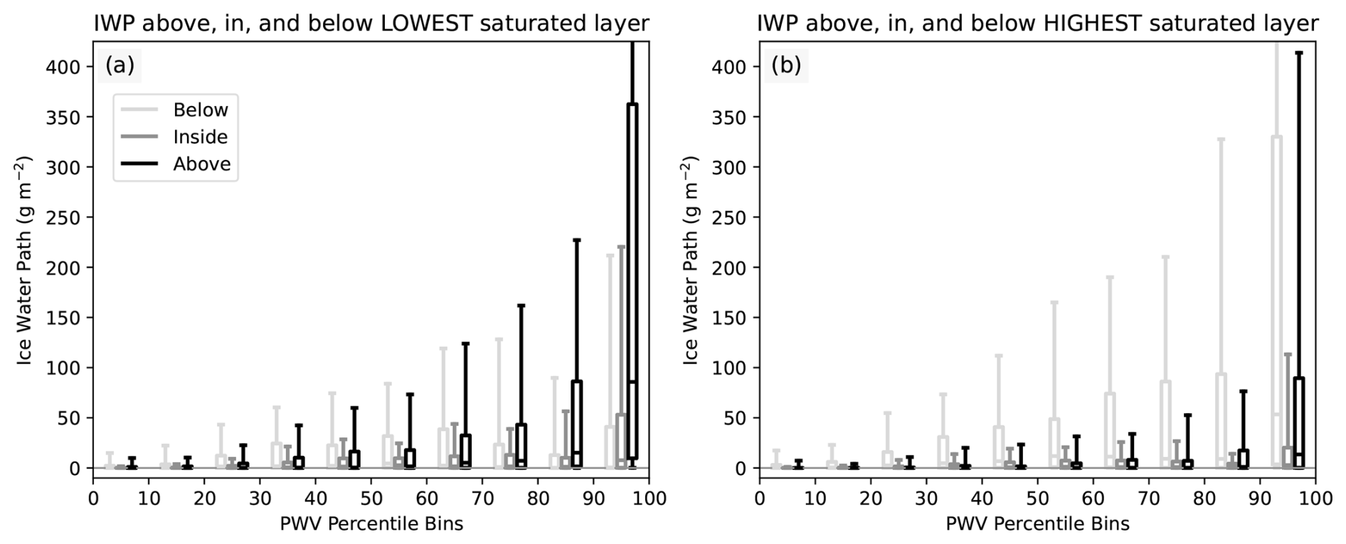
Figure A10 Distributions, by PWV percentile bin, of the total ice water path above (black), inside (grey), and below (light grey) the lowest (a) and highest (b) saturated layer.

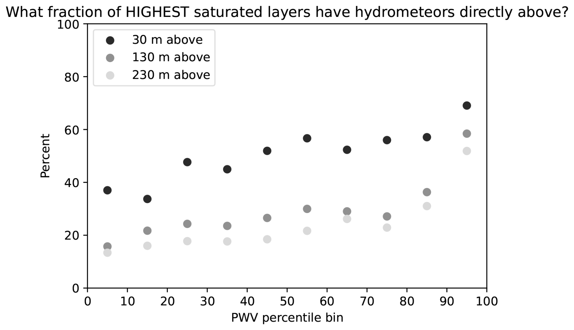
Figure A11 Fraction of the highest saturated layers, by PWV percentile bin, that have radar-detected hydrometeors at three heights directly above saturated layer top.