Methane fluxes from Arctic & boreal North America: comparisons between process-based estimates and atmospheric observations

Methane (CH₄) flux estimates from high-latitude North American wetlands remain highly uncertain in magnitude, seasonality, and spatial distribution. In this study, we evaluate a decade (2007–2017) of CH₄ flux estimates by comparing 16 process-based models with atmospheric CH₄ observations collected from in situ towers. We compare the Global Carbon Project (GCP) process-based models with a model inter-comparison from a decade earlier called The Wetland and Wetland CH₄ Intercomparison of Models Project (WETCHIMP). Our analysis reveals that the GCP models have a much smaller inter-model uncertainty and have an average magnitude that is a factor of 1.5 smaller across Canada and Alaska. However, current GCP models likely overestimate wetland fluxes by a factor of two or more across Canada and Alaska based on tower-based atmospheric CH₄ observations. The differences in flux magnitudes among GCP models are more likely driven by uncertainties in the amount of soil carbon or spatial extent of inundation than in temperature relationships, such as Q₁₀ factors. The GCP models do not agree on the timing and amplitude of the seasonal cycle, and we find that models with a seasonal peak in July and August show the best agreement with atmospheric observations. Models that exhibit the best fit to atmospheric observation also have a similar spatial distribution; these models concentrate fluxes near Canada's Hudson Bay Lowlands. Current, state-of-the-art process-based models are much more consistent with atmospheric observations than models from a decade ago, but our analysis shows that there are still numerous opportunities for improvement.

1 Introduction

Natural sources of CH₄ contribute ∼40 % of total global fluxes, and wetlands are possibly the largest single source (e.g., Kirschke et al., 2013; Saunois et al., 2025). Understanding the magnitude, seasonality, and spatial distribution of wetland CH₄ fluxes is important to accurately predicting future carbon-climate feedbacks. However, the response of wetland CH₄ fluxes to temperature changes is uncertain (e.g., Zhang et al., 2023, 2017), especially in high-latitude regions where warming occurs 2-4 times faster than the global average (e.g., Rantanen et al., 2022).

At least some of this uncertainty is related to uncertain permafrost dynamics. Permafrost covers approximately ∼15 % of the land in the Northern Hemisphere (Obu, 2021), and it serves as a massive reservoir for carbon. Globally, permafrost regions store about 1000 to 1672 peta-grams (Pg) of soil organic carbon (SOC), nearly twice the total amount of carbon in the atmosphere (Schuur et al., 2015; Hugelius et al., 2014; van Huissteden and Dolman, 2012). As permafrost thaws, it changes the soil environment and triggers microbial decomposition of the stored organic matter. When the soil is wet, microbial decomposition in permafrost leads to the release of CH₄ through the process of anaerobic respiration. One study indicates that wetland CH₄ fluxes can be large enough to flip some high latitude regions from a net carbon sink to a net source (Watts et al., 2023).

To understand high-latitude wetland CH₄ fluxes and better predict future warming, process-based (bottom-up) models are important as they can be used to estimate current wetland CH₄ fluxes and project future CH₄ fluxes from regional to global scales, leveraging current scientific knowledge of different biogeochemical processes (e.g., Saunois et al., 2025; Nzotungicimpaye et al., 2021; Melton et al., 2013; Zhang et al., 2017). Despite their importance, the CH₄ flux estimates from bottom-up models can have large discrepancies and uncertainties. For example, bottom-up estimates show that total global wetland fluxes range from 100 to 256 Tg CH₄ yr⁻¹ (Xiao et al., 2024; Zhang et al., 2025; Saunois et al., 2025; Liu et al., 2020). In boreal North America, process-based models also estimate wetland CH₄ fluxes ranging from 13.8 to 39.6 Tg CH₄ yr⁻¹ (Poulter et al., 2017). In addition, a recent study suggests an increase of 50 % to 150 % in global wetland CH₄ fluxes by 2100, a large range of numbers which points to large uncertainties in current projections (Koffi et al., 2020). Model inter-comparison projects like the Wetland and Wetland CH₄ Intercomparison of Models Project (WETCHIMP) have been used to compare the state-of-the-art wetland CH₄ flux models across different regions of the globe (Melton et al., 2013; Wania et al., 2013; Bohn et al., 2015). In more recent years, the Global Carbon Project (GCP) has been created to synthesize scientific knowledge of the global carbon cycle, and this effort includes a large ensemble of the latest process-based CH₄ flux models (Poulter et al., 2017; Zhang et al., 2025). There is limited knowledge on how these models have improved or evolved over time compared to the earlier WETCHIMP inter-comparison. Fortunately, projects like WETCHIMP and GCP make it easier to identify improvements and diagnose uncertainties in wetland flux models because all modeling groups use similar modeling protocols, meteorological inputs, and, in some cases, common inundation or wetland maps. By harmonizing inputs across models, we eliminate input-driven variability due to different climate forcing data, and the remaining model spread therefore primarily reflects differences in process representations and parameterizations.

Numerous studies have also used atmospheric CH₄ to quantify CH₄ fluxes from high-latitude wetlands across North America. Early studies used a sparse network of tower observations in Canada and Alaska to quantify the magnitude, seasonality, and spatial distribution of wetland fluxes (e.g., Worthy et al., 1998; Pickett-Heaps et al., 2011; Miller et al., 2014, 2016a; Karion et al., 2016; Ishizawa et al., 2019). These tower-based studies provide a range of flux estimates from 14.8 to 19.5 Tg CH₄ yr⁻¹ for Canada and 1.56 to 3.4 Tg CH₄ yr⁻¹ for the Hudson Bay Lowlands (HBL), a prominent wetland region in northern Canada (e.g., Ishizawa et al., 2024; Miller et al., 2014; Pickett-Heaps et al., 2011; Thompson et al., 2017). Existing studies using tower-based observations have also commented on inter-annual variability, though these studies disagree on whether high-latitude fluxes have detectable year-to-year variability or a multi-year trend (Ishizawa et al., 2019; Sweeney et al., 2016; Thompson et al., 2017; Ward et al., 2024). Sweeney et al. (2016) argues that there is no multi-decadal trend in CH₄ fluxes using observations from Utqiagvik, Alaska, while inverse modeling studies by Thompson et al. (2017), Ishizawa et al. (2019), and Ishizawa et al. (2024) identify inter-annual variability in wetland fluxes across high-latitude North America.

NASA scientists began collecting intensive aircraft-based greenhouse gas observations across Alaska in 2012, providing a complement to the long-term tower-based network, and these aircraft campaigns have led to a handful of studies on CH₄ fluxes from that state. The authors of these studies quantify the magnitude and spatial distribution of fluxes using inverse modeling (Chang et al., 2014; Miller et al., 2016b; Hartery et al., 2018; Sweeney et al., 2022). These estimates range from 1.48 to 2.6 Tg CH₄ yr⁻¹, a number similar to CH₄ flux totals from Canada's Hudson Bay Lowlands (Miller et al., 2016b; Hartery et al., 2018; Chang et al., 2014; Sweeney et al., 2022). By contrast, the WETCHIMP process-based models span a much wider range from 0.65 to 6.0 Tg CH₄ yr⁻¹, a nearly nine-fold spread.

Several studies also leverage aircraft observations to conduct a detailed evaluation of flux processes and of numerous process-based models, mostly from the WETCHIMP inter-comparison (Miller et al., 2016b; Hartery et al., 2018). For example, these inverse modeling estimates indicate that tundra ecosystems contribute a disproportionate share of Alaskan CH₄ fluxes (often >50 % of total Alaskan CH₄ fluxes despite their smaller areal extents). The North Slope alone accounts for ∼24 % of the total statewide CH₄ fluxes, which is ∼20 % higher than the estimates of process-based models (Miller et al., 2016b; Hartery et al., 2018). Collectively, these aircraft-based studies demonstrate that process-based flux estimates not only diverge substantially from one another, but also from atmospheric constraints. The main driver of this divergence is how models represent wetland extent and water table dynamics, and these factors have a salient influence on the magnitude and spatial distribution of high-latitude wetland CH₄ fluxes estimated by process-based models (Miller et al., 2016b). Hartery et al. (2018) also argue that in wetland soils, CH₄ fluxes are likely driven by near-surface soil temperature and moisture while fluxes from non-wetland soils are more likely driven by temperature and moisture at greater depths, a difference in processes that may be key for effectively modeling CH₄ fluxes across Alaska.

Since the early 2010s, the tower-based observing network has greatly expanded across high-latitude North America, providing a new opportunity to evaluate process-based models and to suggest future opportunities for improvement. In addition, we can now compare two different process-based model ensembles, generated over a decade apart, to assess how process-based estimates of high-latitude wetland fluxes have evolved over time (i.e., the WETCHIMP and GCP ensembles). In this study, we use atmospheric CH₄ observations from tower sites to evaluate the GCP process-based models across high-latitude North America. We specifically use four sets of analyses to compare atmospheric CH₄ observations and the GCP wetland flux models with a goal of suggesting future improvements to these models. For each of these analyses, we run each GCP flux estimate through an atmospheric transport model to simulate atmospheric CH₄, and we compare the results against available atmospheric CH₄ observations. First, we compare the GCP models across high latitudes against the WETCHIMP models and explore how process-based flux models have evolved over the past decade. Second, we examine how the GCP models vary in CH₄ flux magnitude and what potential factors might drive agreement or disagreement among the models. Third, we investigate differences in seasonal cycles across models that best match atmospheric observations versus models that show seasonal discrepancies with atmospheric observations. Lastly, we examine the spatial distribution of the CH₄ fluxes estimated by the GCP models and identify spatial patterns that appear to yield better agreement with the available atmospheric CH₄ data.

2 Data and methods

2.1 Atmospheric CH₄ Measurements

To better understand current wetland CH₄ fluxes, we compare GCP CH₄ flux estimates with 11 years of in situ tower data from the United States and Canada, spanning 2007 to 2017. We note that several previous studies have already used intensive aircraft campaigns to examine CH₄ fluxes across specific regions of Alaska and to evaluate process-based flux models in those regions (e.g., Miller et al., 2016b; Hartery et al., 2018; Chang et al., 2014; Sweeney et al., 2022). We build upon these existing studies by evaluating process-based models using long-term tower observation sites that are distributed cross both Canada and Alaska, and we compare and contrast our results with previous aircraft-based studies in the Results and discussion section (Sect. 3).

We also focus on the months of May through October each year. Wetland CH₄ fluxes are largest during these months, and many existing top-down studies have focused on these months for their analyses (e.g., Miller et al., 2016b; Chang et al., 2014; Pickett-Heaps et al., 2011). By contrast, the ratio of wetland fluxes to anthropogenic CH₄ emissions is much smaller in other months of the year across Alaska and Canada, making it more difficult to uniquely constrain wetland fluxes using atmospheric observations. The geographic domain of this study covers the high-latitude regions of North America, ranging from 40 to 80° N and 170 to 50° W.

The atmospheric data used in this study come from the NOAA Observation Package (ObsPack) CH₄ GlobalViewPlus v5.1 dataset (Di Sarra et al., 2023). There are 21 available tower sites within the study domain, and the towers provide a combination of continuous and flask measurements. We list a more detailed description of each tower site and its location in Table S1 in the Supplement. In addition, we extract afternoon averages of the observations between 01:00 p.m. and 06:00 p.m. local time when the boundary layer is generally well-mixed, and we do this to reduce transport uncertainties in STILT. During this time of day, CH₄ measurements are arguably influenced by fluxes from a broader region than at night. By contrast, the atmosphere is usually stable in the morning and at night with lower boundary layer heights, making accurate atmospheric trace gas modeling challenging. As a result, we prioritize robust transport over full diurnal coverage, and this approach is similar to multiple existing top-down studies (e.g., Miller et al., 2014, 2016a; Karion et al., 2016; Ishizawa et al., 2024).

2.2 Wetland CH₄ flux model ensembles: GCP and WETCHIMP

The Global Carbon Project (GCP) includes global-scale wetland CH₄ flux models that use diverse hydrological and biogeochemical schemes (Zhang et al., 2025). The most recent GCP model ensemble includes 16 process-based models spanning the period from 2000 to 2020, though some models end earlier or later than 2020. A general description of these GCP models is provided in Table S2 and in Zhang et al. (2025). Each of the these models is run in two different ways: diagnostically and prognostically. The diagnostic runs for each model are constrained by a predefined inundation map from the product Wetland Area and Dynamics for Methane Modeling version 2 (WAD2Mv2), while the prognostic runs estimate the inundation internally using their own hydrological schemes such as soil moisture (Zhang et al., 2021). As a result, prognostic inundation is not observation-driven, and inter-model differences are driven by the hydrological scheme and climate forcing. Note that each GCP modeling group did not submit variables like soil carbon, and this fact limits our ability to diagnose disagreements in the CH₄ flux estimates from different models. More detailed descriptions of the current GCP model ensemble, including their approaches to wetland inundation and model parametrization can be found in Zhang et al. (2025).

In this study, we evaluate the 11 prognostic and 16 diagnostic models included in the GCP ensemble. Each of these models was run using two different meteorological reanalysis products to examine the effects of meteorological uncertainties on estimated CH₄ fluxes. These products include the Global Soil Wetness Project Phase 3 (GSWP3) and the Climate Research Unit (CRU) Time-Series 4.06 (Harris et al., 2022; Lange and Büchner, 2020). A recent study shows that the differences between these two climate-forcing datasets are negligible (Ito et al., 2023). Nevertheless, both datasets are included in this study to provide a comprehensive evaluation.

We also evaluate process-based wetland CH₄ fluxes using the Wetland and Wetland CH₄ Intercomparison of Models Project (WETCHIMP), which is designed to compare modeled monthly CH₄ fluxes across the globe between 1993 and 2004 (Melton et al., 2013; Wania et al., 2013). There are seven models available that provide CH₄ fluxes in the North America domain. These models are CLM4Me (Riley et al., 2011), DLEM (Tian et al., 2010), LPJ-Bern (Spahni et al., 2011), LPJ-WHyMe (Wania et al., 2010), LPJ-WSL (Hodson et al., 2011), ORCHIDEE (Ringeval et al., 2010), and SDGVM (Singarayer et al., 2011).

We regrid the GCP and WETCHIMP models into an uniform spatial resolution of 1° latitude by 1° longitude. This regridding process is performed using the “remapcon” function from the Climate Data Operators (CDO) software, which conserves the total fluxes of each model during interpolation (Schulzweida, 2023).

2.3 Anthropogenic CH₄ emissions

We include three distinct combinations of anthropogenic CH₄ flux products to highlight the variability and uncertainty in our analysis due to anthropogenic CH₄ fluxes. Bottom-up inventories such as Canada's National Inventory Report (NIR) estimate total anthropogenic fluxes of approximately 3.7 Tg CH₄ yr⁻¹ (Scarpelli et al., 2021). In contrast, top-down inverse modeling and observation-constrained studies generally infer higher national totals, on the order of 5 to 7 Tg CH₄ yr⁻¹ (e.g., Thompson et al., 2017; Lu et al., 2022; Chan et al., 2020; MacKay et al., 2021; Ishizawa et al., 2024). Existing bottom-up and top-down studies show particularly large discrepancies in oil and gas producing regions of western Canada (Ishizawa et al., 2024; Chan et al., 2020; MacKay et al., 2021; Baray et al., 2021). Collectively, the spread among bottom-up and top-down studies highlights the large uncertainty in Canadian anthropogenic CH₄ flux estimates and underscores the importance of exploring multiple flux products in our analysis.

We use three specific anthropogenic flux products and regrid them to a spatial resolution of 1° latitude by 1° longitude for the study domain, and we aggregate them to a monthly temporal resolution for 2007–2017:

1. CarbonTracker CH₄ 2023 (Oh et al., 2023): CarbonTracker is an inverse modeling system designed to estimate CH₄ fluxes on a global scale (Oh et al., 2023).

2. A combination of the gridded U.S. Greenhouse Gas Inventory (Version 2) and a gridded inventory of Canada's anthropogenic CH₄ fluxes (Maasakkers et al., 2023; Scarpelli et al., 2021): Scarpelli et al. (2021) constructed a gridded Canadian anthropogenic flux inventory based on the Canadian National Inventory Report (NIR), the Canadian Greenhouse Gas Reporting Program (GHGRP), and other datasets to provide a detailed sectoral breakdown of fluxes. Similarly, Maasakkers et al. (2023) created a U.S. gridded inventory integrating data from the U.S. Environmental Protection Agency's (EPA) Greenhouse Gas Inventory (GHGI) to provide fluxes from different sectors.

3. The Copernicus Atmosphere Monitoring Service (CAMS) (Granier et al., 2019): CAMS is a global inverse modeling system that provides estimates of global atmospheric CH₄ fluxes and atmospheric mixing ratios. This product is derived from a combination of the Emissions Database for Global Atmospheric Research (EDGARv4.3.2) and Community Emissions Data System (CEDSv3) inventories, and the product includes estimates of fluxes from different source sectors (Granier et al., 2019).

2.4 Atmospheric modeling

We use the WRF-STILT (The Weather Research and Forecasting-Stochastic Time-Inverted Lagrangian Transport) to simulate the atmospheric transport of CH₄ fluxes, which has been widely used in numerous studies of regional greenhouse gas fluxes (e.g., Miller et al., 2016b; Henderson et al., 2015; McKain et al., 2015; Kort et al., 2010; Feng et al., 2023; Miller et al., 2014). STILT is a Lagrangian particle dispersion model that simulates atmospheric transport using an ensemble of tracer particles (Lin et al., 2003). For the setup here, the model releases those particles from each measurement site, and the particles travel backward in time for 10 d following the wind fields in WRF meteorology. STILT uses these particle trajectories to calculate surface influence maps or footprints for each atmospheric CH₄ observation (Fig. 1). These footprint maps have units of mixing ratio per unit flux (ppb per $\mathrm{\mu }\mathrm{mol}{\mathrm{m}}^{-\mathrm{2}}{\mathrm{s}}^{-\mathrm{1}}$) on a 1° by 1° grid. We can directly multiply these footprints by CH₄ fluxes from the process-based models to predict atmospheric CH₄ mixing ratios at each tower site. The footprints used in this study were generated as part of the NOAA CarbonTracker-Lagrange project and are available from 2007 to 2017, which defines our study time frame (Hu et al., 2019).

Since CH₄ has an atmospheric lifetime of about 10 years, it can remain in the atmosphere and travel around the globe. To account for the large-scale movements of CH₄, we estimate CH₄ boundary conditions using CH₄ observations collected over the Pacific and Atlantic oceans, from high-altitude tower sites in the continental US, and from regular aircraft flights across the US and Canada. We use these observations to interpolate a curtain of CH₄ mixing ratios around the boundaries of the model domain. For each STILT simulation, we sample from this boundary condition curtain based on the ending locations of the particle trajectories. This procedure thus accounts for CH₄ that enters the domain from other regions of the globe. The approach used here is identical to that used in numerous existing regional CH₄ studies (e.g., Miller et al., 2013, 2014, 2016a).

We note that the STILT particle trajectories used here from CarbonTracker-Lagrange do not include atmospheric oxidation processes. However, CH₄ oxidation by hydroxyl radicals likely has a small impact in our study given the short, 10 d time frame of the regional STILT simulations used here. For example, Miller et al. (2013) argue that CH₄ mixing ratios decay less than 1 to 1.5 ppb over the first 2–3 d of STILT back trajectories given the average global-averaged lifetime of CH₄ of 7–11 years. This corresponds to less than 5 % of the average modeled CH₄ mixing ratio enhancement relative to background in our study. The impact of OH in our study may be even smaller because OH mixing ratios are usually lower at high latitudes compared to the continental US. In addition, our estimated boundary conditions also account for long-range CH₄ oxidation processes that occur upwind of our domain.

We combine the aforementioned modeling components using the following equation to compare atmospheric CH₄ observations with the STILT model predictions using the GCP flux models:

$$\begin{array}{}\text{(1)}& \mathit{Z}\sim \mathbf{H}\left[\mathit{s}+\mathit{A}+\mathit{B}\right]+\mathit{b}.\end{array}$$

where Z represents the atmospheric observations from the in situ towers across the US and Canada (dimensions n×1, where n are the number of observations). H is a matrix of influence footprints assembled from the WRF-STILT model (dimensions n×m, where m is the number of flux model grid boxes in space and time). Within the brackets, s refers to wetland CH₄ flux estimates from the process-based GCP or WETCHIMP models (dimensions m×1, Sect. 2.2), A refers to the anthropogenic CH₄ fluxes estimate from one anthropogenic product (dimensions m×1, Sect. 2.3), and B denotes biomass burning fluxes from the Global Fire Emissions Database (GFED v4.1) (Randerson et al., 2017) (dimensions m×1). The last variable, b, represents the CH₄ boundary condition (dimensions n×1).

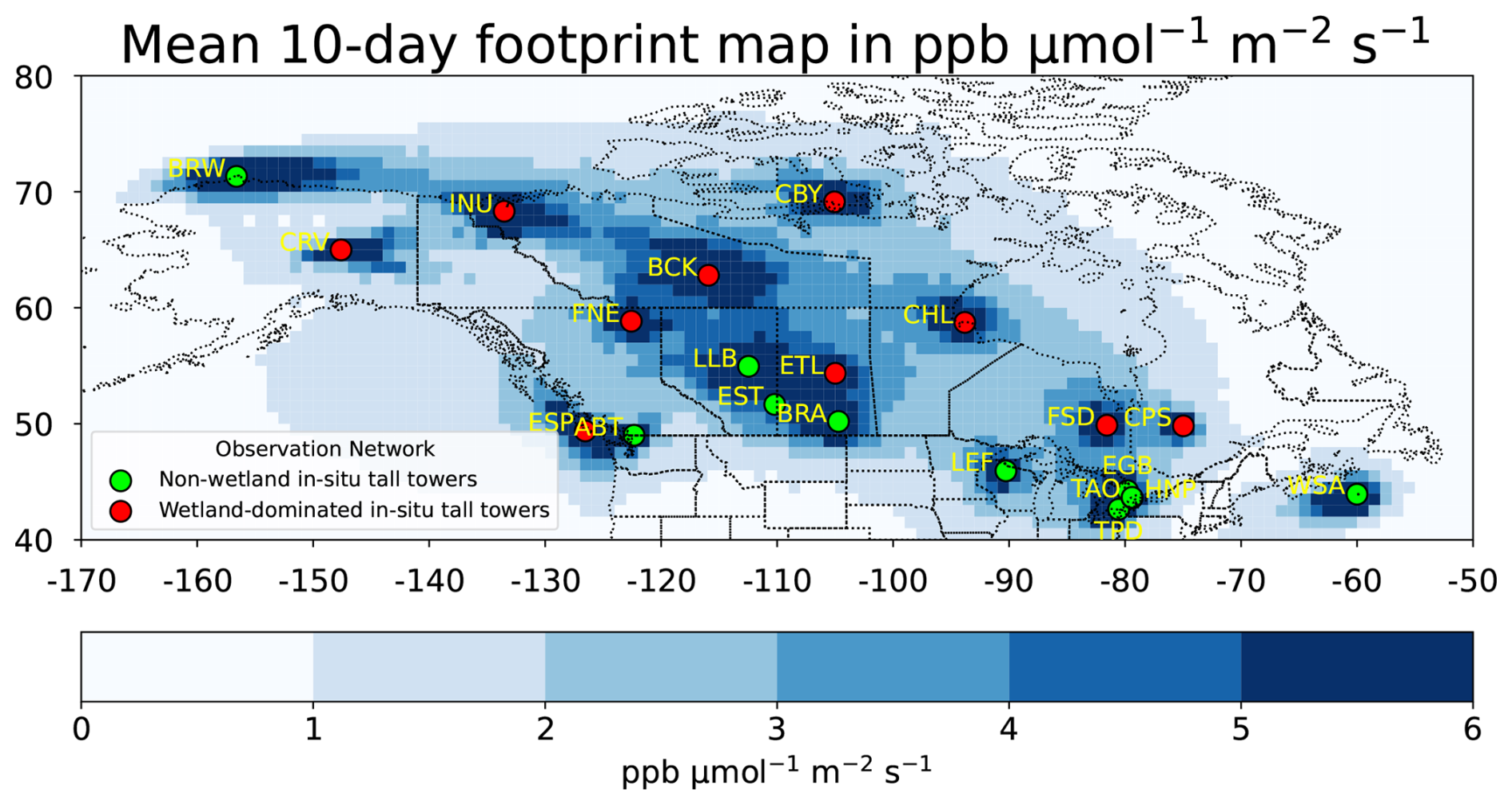
Figure 1 The US and Canadian atmospheric CH₄ observing network from 2007–2017. The figure also shows the WRF-STILT mean 10 d footprint map in $\mathrm{ppb}(\mathrm{\mu }\mathrm{mol}{\mathrm{m}}^{-\mathrm{2}}{\mathrm{s}}^{-\mathrm{1}}{)}^{-\mathrm{1}}$ across the study domain of 40 to 80° N and 170 to 50° W, and footprints are evaluated from 2007–2017. Red circle dots show in situ tall tower sites from NOAA and Environmental Canada from the ObsPack GlobalViewPlus v5.1 dataset (Di Sarra et al., 2023). The lime-colored dots represent non-wetland sites, where the wetland-to-anthropogenic CH₄ concentration ratio is less than 1.3 (using anthropogenic emissions from the CAMS product). In contrast, the red-colored dots indicate wetland-dominated sites, where this ratio exceeds 1.3.

We run STILT simulations both with and without the lake and reservoir emissions from Maasakkers et al. (2016), which contribute approximately 0.72 Tg CH₄ yr⁻¹ in Canada from May to October. The WAD2M v2 inundation map (used by GCP models) represents vegetated wetlands only, but small lakes and ponds could still overlap because these features are difficult to distinguish from wetlands in satellite observations (Kyzivat and Smith, 2023). Adding a separate lake component could therefore lead to partial double-counting of freshwater emissions and further increase the modeled CH₄ mixing ratios. Given this potential for double-counting, we present results without the additional lake term, while we acknowledge that adding lake and reservoir emissions would further increase modeled CH₄ mixing ratios.

Note that we only include observation sites in our analysis if those sites are predominantly influenced by CH₄ fluxes from wetlands. By contrast, we exclude urban sites and sites proximal to oil and gas operations. We specifically include sites where the average ratio of modeled CH₄ from STILT using the GCP model mean to modeled CH₄ using the CAMS anthropogenic flux product is greater than 1.3 (Sect. 2.4, 2.2, 2.3). This screening means that the wetland contributions at each site are at least 30 % higher than the likely influence of anthropogenic emissions. If we set a lower threshold, then we would begin to include sites in urban and/or oil and gas producing areas. For example, the site with the next highest wetland-to-anthropogenic ratio is Abbotsford (ABT), which is an urban site near Vancouver, British Columbia. By contrast, if we set a higher threshold, we would exclude the East Trout Lake (ETL) tower site, which is located in a sparsely populated wetland region of northern Saskatchewan. We focus on these sites because we aim to better quantify the contribution of wetlands to atmospheric CH₄ levels while minimizing the confounding effects of anthropogenic sources, the magnitudes of which are also uncertain. The ten sites that we include within this study are Churchill, Manitoba (CHL); Cambridge Bay, Nunavut (CBY); East Trout Lake, Saskatchewan (ETL); Estevan Point, British Columbia (ESP); Fort Nelson, British Columbia (FNE); Fraserdale, Ontario (FSD); Inuvik, Northwest Territories (INU); Behchoko, Northwest Territories (BCK); Chapais, Quebec (CPS); and the Carbon in Arctic Reservoirs Vulnerability Experiment Tower, Fairbanks, Alaska (CRV) (see Table S1 for additional details). The remaining sites that are not included in this analysis are towers in urban environments (e.g., sites in the Toronto and Vancouver metropolitan areas); towers close to oil and gas production in Alberta, Canada, or Prudhoe Bay, Alaska; towers that are frequently used as clean air background sites (e.g., Sable Island, Nova Scotia), and sites proximal to intensive agriculture.

3 Results and discussion

In this section, we compare the modeled CH₄ mixing ratios using the GCP models to atmospheric observations. We use these comparisons to evaluate the magnitude, seasonality, and spatial distribution of the GCP flux models over 2007 to 2017. In each subsection, we also speculate on the possible reasons driving the agreement or disagreements that we see in our analyses.

3.1 Comparisons between the GCP and WETCHIMP models

The GCP model ensemble is an updated version of the earlier WETCHIMP inter-comparison over a decade ago (Melton et al., 2013; Wania et al., 2013). Overall, we find that, compared to the WETCHIMP models, the GCP models have a smaller flux magnitude with reduced inter-model spread and better inter-model agreement on the spatial distribution of fluxes within our study domain.

We find that the CH₄ flux estimates from the GCP models are much smaller across most of high-latitude North America compared to the WETCHIMP models. We calculate annual CH₄ flux totals for Canada using the 11 prognostic and 16 diagnostic GCP models with both climate forcing datasets (GSWP3 and CRU), and the uncertainty bars in Fig. 2 represent the standard deviation of the CH₄ flux estimates among models within the same group. The mean annual CH₄ flux total for Canada using the 11 prognostic GCP models with CRU is 14.19±7.41 Tg CH₄ yr⁻¹, and the mean using the 16 diagnostic models with CRU is 12.17±5.48 Tg CH₄ yr⁻¹ (Fig. 2). In contrast, the Canadian annual CH₄ flux total using all the WETCHIMP models with CRU meteorology is a factor of more than ∼1.5 higher than the prognostic and diagnostic GCP models, with flux estimates of 21.50±15.12 Tg CH₄ yr⁻¹ (based on the standard deviations of models within the same group). In Alaska, the annual CH₄ flux total estimated by the 11 prognostic GCP models with CRU is 1.31±0.85 Tg CH₄ yr⁻¹, whereas the seven WETCHIMP models yield a higher value of 1.66±2.02 Tg CH₄ yr⁻¹. We notice that the annual Canadian CH₄ flux total for the LPJ-WHyMe model from WETCHIMP is 46.25±5.88 Tg CH₄ yr⁻¹ (Fig. S5). We subsequently exclude this model and recalculate the annual CH₄ flux total using the other six WETCHIMP models, and evaluate whether or not it brings the flux estimates similar to the GCP models. However, the annual CH₄ flux total using the other six WETCHIMP models with CRU is 17.97±12.59 Tg CH₄ yr⁻¹, which is still about a factor of ∼ 1.4 higher than the prognostic GCP models using CRU meteorology.

In addition, the annual CH₄ flux totals estimated by the WETCHIMP models are a factor of ∼1.3 or higher than the GCP models in the two dominant high-latitude biomes across North America (tundra and boreal forests) (Fig. 2). Across the North American boreal forests and tundra, the annual CH₄ flux totals estimated by the 11 prognostic GCP models with CRU are 10.71±5.73 and 1.64±1.31 Tg CH₄ yr⁻¹, respectively. In comparison, the annual CH₄ flux totals estimated by the seven WETCHIMP models in these two biomes are 16.62±8.55 and 2.15±1.34 Tg CH₄ yr⁻¹, respectively.

We also find that the CH₄ fluxes estimated by the 11 prognostic GCP models result in much lower inter-model uncertainty compared to the seven WETCHIMP models, with smaller inter-model disagreement across Canada and southern Alaska. Here, we define the uncertainty among models as the standard deviation across the models of the mean wetland flux CH₄ in May–October. To evaluate model agreement on the spatial distribution of fluxes, we compare the inter-model uncertainty or the standard deviation of flux estimates for each individual model grid box of the GCP and WETCHIMP models. Since each WETCHIMP model identifies the inundation or wetland area differently, we compare these models with the prognostic GCP models (Melton et al., 2013). Note, however, that not all of the WETCHIMP modeling groups generated their own wetland or inundation maps prognostically, and some, like LPJ-Bern and LPJ-WHyMe, use a constant, prescribed wetland map. In Fig. 3, darker shades represent higher inter-model uncertainty across these process-based models. We observe that the GCP models have much lighter shades across the study domain, indicating better inter-model agreement.

We further find that the WETCHIMP models generally exhibit seasonal cycles that are similar to the GCP models (Fig. S1a and b). Most WETCHIMP models estimate peak CH₄ fluxes across Alaska and Canada in July and August, except CLM4Me (which peaks in June) and LPX-Bern (which peaks in September). This result illustrates that the seasonal cycles of the GCP models have not changed markedly from the WETCHIMP models. The WETCHIMP models already showed relatively good agreement on the seasonal cycle of fluxes, but such agreement does not guarantee accuracy, and there remains scope for improvement. Furthermore, the seasonal cycle of these model estimates is likely dependent on temperature, meaning that it is arguably easier to model than other features that depend on more complex processes.

The overall reduction in inter-model uncertainties from WETCHIMP to GCP may relate to how the models estimate wetland distribution. Different WETCHIMP model yield very different estimates of maximum wetland extent – from 2.7 to 36.4×10⁶ km² for the global extra-tropics (>35° N), depending upon the model. Melton et al. (2013) explain that several WETCHIMP models use a binary approach to identify wetland areas, where individual model grid boxes are either 100 % wetland or 0 % wetland, and these models tend to have ∼3–4 times greater wetland area compared to other models (Fig. 2 and Table 2 in Melton et al., 2013). Other WETCHMIMP models were parameterized to match remote sensing estimates of wetland or open water extent. In contrast to WETCHIMP, the GCP model ensemble also includes diagnostic experiments in which all modeling groups used the WAD2M v2 inundation map. These efforts to create a standardized, diagnostic map of wetland extent may have also influenced the prognostic GCP experiments, and modeling groups may have tuned or modified their setup to be more consistent with the diagnostic model simulations. In addition, the lower magnitude of CH₄ fluxes estimated by the GCP models (compared to the WETCHIMP models) is partly attributed to efforts by the GCP modeling group to reduce double-counting of freshwater areas (e.g., lakes and ponds) in WAD2M v2 (Zhang et al., 2021).

Note that the GCP models show lower flux magnitude and reduced inter-model spread in Canada, even when using the subset of models that are common to both WETCHIMP and GCP. For diagnostic GCP runs, the overlapping model subsets with WETCHIMP are LPX-Bern (a newer version of LPJ-Bern), DLEM, ORCHIDEE, LPJ-wsl, SDGVM. For prognostic GCP runs, the common models include LPX-Bern, ORCHIDEE, LPJ-wsl, and SDGVM. Using these shared models, we find that the mean annual flux total from the WETCHIMP models is roughly 4 Tg CH₄ yr⁻¹ higher than the matched GCP ensemble mean, whereas in Alaska WETCHIMP is 0.11 Tg CH₄ lower (Figs. S5 and S6). In addition, we also find that the GCP ensemble exhibits lower inter-model spread in Canada and broadly similar or lower spread in Alaska (Fig. S9). As a result, these analyses lead to the conclusion that the GCP ensemble is more tightly constrained than WETCHIMP over Canada when the same models are compared.

The reduced inter-model spread indicates greater consistency among the current GCP model outputs relative to WETCHIMP; however, reduced spread alone does not indicate improved accuracy. In the following sections, we compare the GCP and WETCHIMP models with atmospheric observations to gauge whether the GCP models are indeed more skilled at capturing CH₄ fluxes across high-latitude North America.

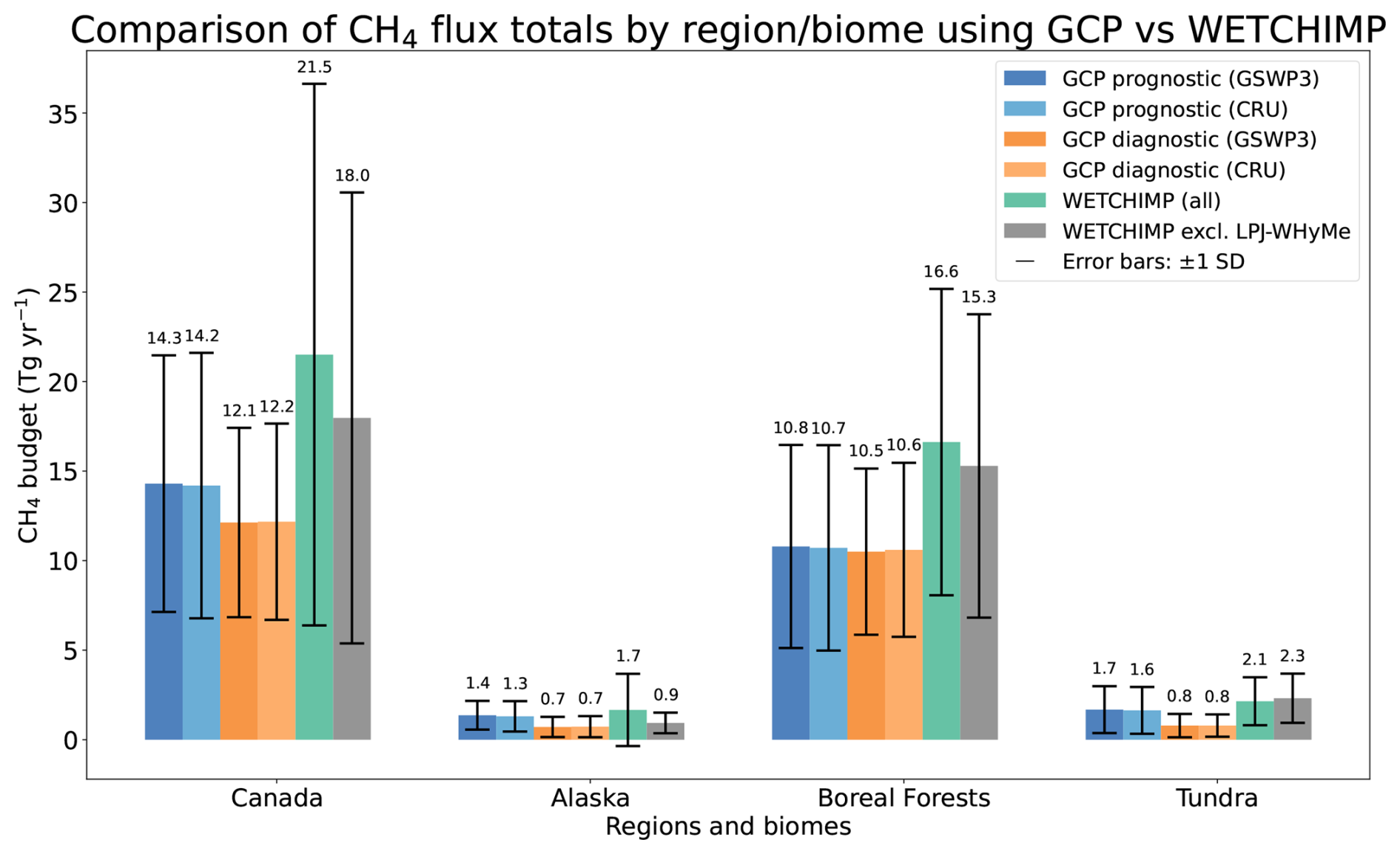
Figure 2 Annual CH₄ flux totals across Canada, Alaska, and several biomes. The four bars on the left of each region or biome represent the 2 different climate forcing data (GSWP3 and CRU) and prognostic versus diagnostic types for the GCP models. The green bar shows the mean annual CH₄ flux total using all WETCHIMP models, and the gray bar denotes the mean flux total excluding the LPJ-WHyMe model. The uncertainty bars represent the standard deviation of the CH₄ flux estimates among models within the same group. The unit of the annual wetland CH₄ flux totals is Tg CH₄ yr⁻¹.

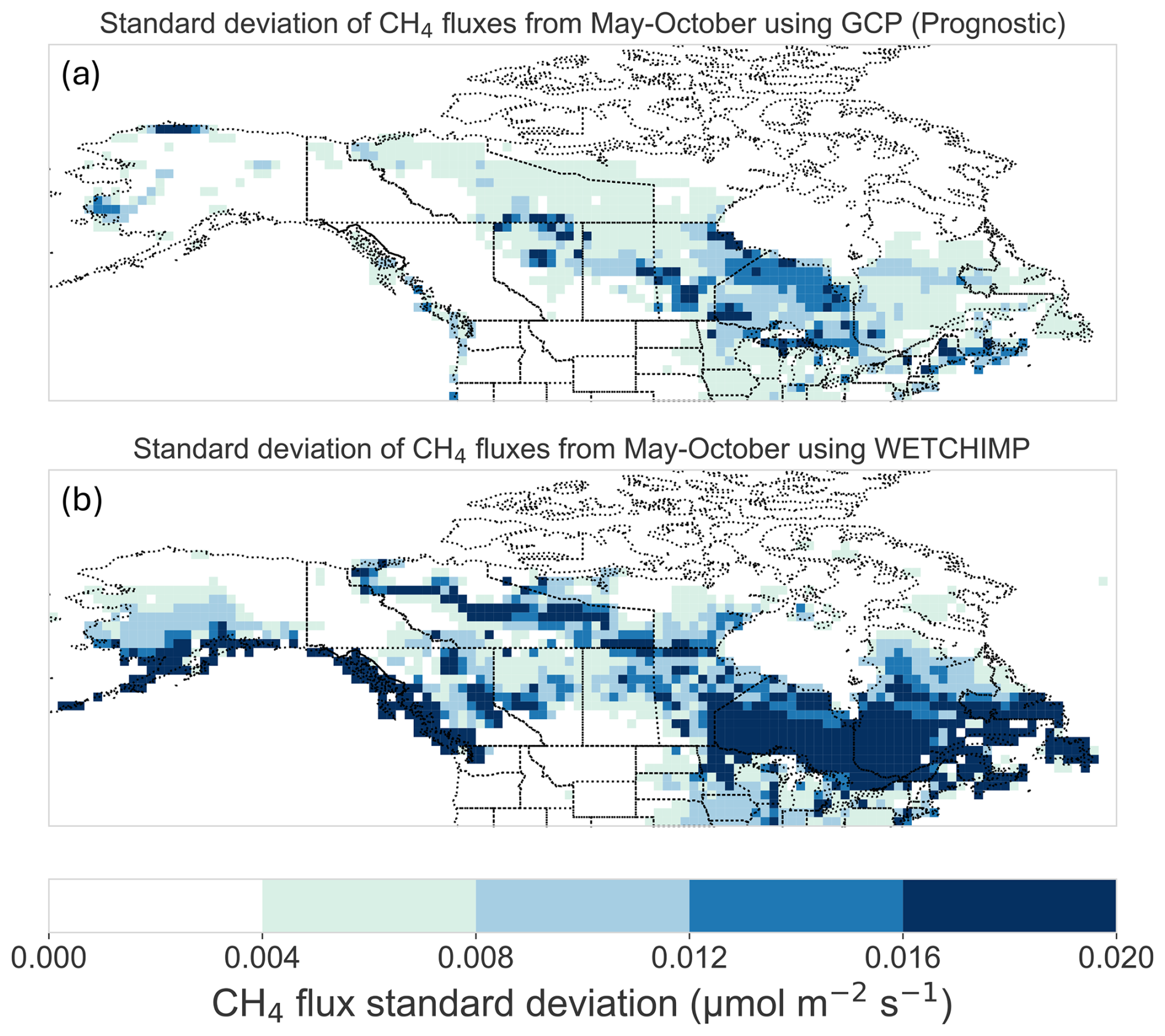
Figure 3 The inter-model standard deviation for each individual model grid box, calculated using the 11 prognostic GCP models (top) and WETCHIMP models (bottom). The inter-model uncertainty is higher for the WETCHIMP models than the GCP models. All fluxes have units $\mathrm{\mu }\mathrm{mol}{\mathrm{m}}^{-\mathrm{2}}{\mathrm{s}}^{-\mathrm{1}}$.

3.2 Flux magnitude

We find that even though the mean wetland CH₄ fluxes of the GCP models are about a factor of two lower than the WETCHIMP models across northern North America, most of them are still likely an overestimate by a factor of two or more compared to atmospheric CH₄ observations (Fig. 4). Note that we exclude lake and reservoir emissions from the following results because adding these emissions could double-count existing freshwater sources already represented in WAD2M v2 and further increase the modeled CH₄ mixing ratios relative to our current results.

We evaluate the magnitude of the GCP models by comparing modeled mixing ratios from STILT against observations at the tower sites. Specifically, we divide modeled CH₄ mixing ratios using wetland fluxes from the GCP models by the observed increments, shown in Fig. 4. The modeled wetland CH₄ mixing ratios are calculated by passing each of the GCP models through WRF-STILT. The observed increments are calculated as the atmospheric CH₄ observations minus factors unrelated to wetlands – the CH₄ boundary condition and the contributions of anthropogenic and biomass burning fluxes at the observation sites. In Fig. 4, we compare the magnitude of the modeled wetland CH₄ mixing ratios and the observed increments at each wetland-dominated in situ tower site across high-latitude North America. A factor larger than one means that the mixing ratios of modeled wetland CH₄ using the GCP models are higher than the observed increments. By contrast, the gray dashed line at the y axis equal to 1 indicates a perfect alignment between the modeled wetland CH₄ mixing and the observed increment. The error bars in Fig. 4 reflect the range of results when we use different anthropogenic flux estimates in the calculations (Sect. 2.3). Note that CH4MOD, DLEM, LPJ-GUESS, TEM-MDM, and TRIPLEX-GHG only have diagnostic simulations and not prognostic simulations, and their diagnostic comparisons are represented exclusively by orange bars.

Interestingly, this result is not geographically uniform across high-latitude North America; the GCP models, when passed through the WRF-STILT transport model, overshoot observations at towers in the boreal zone but not at towers in the Arctic (Fig. S4). This result parallels earlier studies that use intensive aircraft campaign data from specific regions of Alaska. For example, Miller et al. (2016b) estimate CH₄ fluxes over Alaska's North Slope that exceed most process-based model estimates but find substantially lower fluxes than the model estimates across interior boreal and subarctic southeastern Alaska. Similarly, Hartery et al. (2018) emphasize the disproportionately large contribution of Arctic Alaska to the state's total CH₄ fluxes, though they do not explicitly compare their results with process-based models. Global inverse models, like those included in the most recent Global Carbon Project CH₄ report, further reiterate these results; most yield lower wetland CH₄ fluxes across global high latitudes compared to process-based models, including across Russia, Europe, Canada, and the US (Saunois et al., 2025).

We also note that anthropogenic CH₄ fluxes pose an enormous challenge for isolating and quantifying CH₄ fluxes from wetlands, even at very remote observation sites in Canada and Alaska. The vertical bars in Fig. 4 indicate uncertainties in the results due to uncertain anthropogenic fluxes, and we observe a broad spectrum of values depending on which anthropogenic CH₄ flux estimate we use. For example, modeled mixing ratios from STILT using the GCP CH₄ model CLASSIC run prognostically are anywhere between ∼2.5 times higher than the observed increment to ∼6 times higher, depending on the choice of anthropogenic flux product. As a result, we cannot precisely constrain the optimal magnitude of wetland fluxes. These uncertainties notwithstanding, our findings still suggest that wetland fluxes estimated by the 11 prognostic and 16 diagnostic models are often higher than implied by atmospheric observations.

It is difficult to determine the specific causes that drive model disagreements over the magnitude of wetland CH₄ fluxes. However, these variations are more likely influenced by factors such as soil carbon or by the simplicity/complexity of the model structure rather than by disagreements over the effects of temperature on fluxes. We do not have a comprehensive set of modeled environmental variables (e.g., soil carbon) to conduct a systematic examination of all sources of uncertainty. However, the available model outputs allow us to reason through some key contributors to these uncertainties, such the relationships between fluxes and temperature (i.e., estimated Q₁₀ values) and the effects of using a common diagnostic inundation map versus prognostically generated inundation.

To explore the temperature sensitivities of each GCP model, we fit a Q₁₀ curve for each GCP model (Figs. S12–S13). The Q₁₀ parameter represents the sensitivity of wetland CH₄ fluxes to a 10°C increase in temperature, which provides insight into how strongly each model responds to temperature changes. A higher Q₁₀ value indicates that the flux estimates are more prone to change with temperature variations. Our analysis indicates a large variation in temperature sensitivity across the prognostic and diagnostic GCP models, but there is not a strong relationship between the magnitude of wetland CH₄ fluxes estimated by these models and the estimated Q₁₀ values (Figs. S12–S13). As a result, Q₁₀ does not seem to be the most important contributor driving differences in the flux magnitude of the GCP models.

We also find that uncertainties in wetland area and inundation likely contribute to but are not the primary cause of these disagreements in flux magnitude. For example, the prognostic and diagnostic models usually yield a similar magnitude of fluxes, despite of the fact that these different experiments do not use the same inundation estimates (Fig. 2). For Canada, the average total flux from the prognostic models is similar to the diagnostic models – 14.19 and 12.17 Tg yr⁻¹, respectively (using GSWP3 meteorology). Similarly, the average total flux from the prognostic versus diagnostic models is nearly identical for the boreal forest biome. In some regions, the diagnostic models show greater agreement on the total annual flux than the prognostic models, but in other regions, the prognostic and diagnostic models show similar levels of inter-model agreement (Fig. 2).

Interestingly, we find models with simpler flux calculations yield flux magnitudes that agree more with atmospheric observations compared to those using more complex equations. GCP models such as LPJ-wsl, SDGVM, and JULES produce smaller flux magnitudes, and each of these models uses simple approaches to simulate CH₄ fluxes. For example, these models rely only on net fluxes without accounting for specific transport pathways (e.g., ebullition, diffusion, or plant-mediated transport) (Zhang et al., 2025). In contrast, models such as VISIT, JSBACH, and ISAM have the largest flux magnitudes, and these models employ more complex equations that include multiple components of CH₄ fluxes, such as gross production, oxidation, and consumption. These models also simulate explicit transport pathways like ebullition, diffusion, and plant-mediated transport, alongside layered soil temperature schemes for temperature sensitivity (Zhang et al., 2025). Models with more complex representations generally require additional input data to provide more accurate flux estimates. Thus, in data-sparse regions, added process detail could potentially amplify input and parameter uncertainty and enlarge the flux spread.

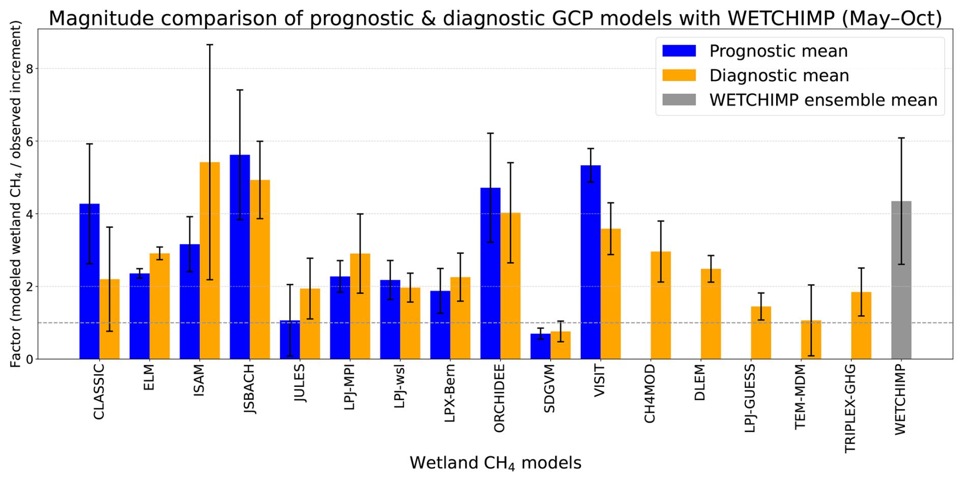
Figure 4 Comparisons between modeled mixing ratios from STILT against observations at the tower sites. The y axis has values range from 0 to 9, representing the ratio between the modeled wetland CH₄ mixing ratios using the GCP and WETCHIMP models and the observed increment. We define the observed increment as the difference between atmospheric CH₄ observations and the sum of the boundary CH₄ levels, modeled anthropogenic CH₄ mixing ratios, and modeled biomass burning CH₄ mixing ratios. A value of 1 on the y axis indicates perfect agreement between the modeled wetland CH₄ mixing ratios and the observed increment.

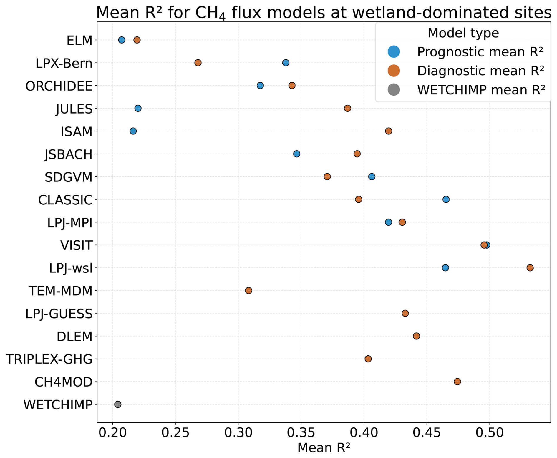
Figure 5 The correlation R² between modeled CH₄ mixing ratios using the process-based models and atmospheric observations. Blue dots represent the mean R² value for prognostic models across different climate forcing data and anthropogenic products. Orange dots represent the mean R² value for diagnostic models across different climate forcing data and anthropogenic products. The gray dot represents the mean R² value for the WETCHIMP models across different anthropogenic products. The y axis lists all the prognostic and diagnostic GCP models and WETCHIMP models, and the x axis shows the R² range for these GCP and WETCHIMP models.

3.3 Seasonality

We find that models more consistent with atmospheric observations have a distinct seasonal peak in wetland CH₄ fluxes in July and August. In contrast, models that do not agree well with atmospheric observations have a flatter seasonal cycle.

To evaluate these differences, we compare the correlation between atmospheric CH₄ observations and STILT simulations using each of the different GCP models (Fig. 5). We specifically use this analysis to explore which GCP models better capture the seasonal and spatial variability of CH₄ fluxes across our model domain. First, we calculate R² values for each model using a two-predictor regression model. In each regression, the first predictor variable represents modeled CH₄ mixing ratios due to wetlands using one of the GCP models, and the second predictor variable represents modeled CH₄ mixing ratios due to different anthropogenic flux products plus biomass burning from GFED (Sect. 2.3 and 2.4). The regression will scale the magnitude of the STILT model outputs to optimally match atmospheric observations. As a result, this analysis is not very sensitive to the absolute magnitude of the original flux estimates. Instead, the overall fit of each regression is more likely a reflection of the seasonal and spatial patterns in the wetland, anthropogenic, and biomass burning flux estimates; GCP flux estimates with more accurate seasonal and spatial variability will more likely yield higher correlation coefficients (R² values). Figure 5 depicts the mean R² values for 16 GCP diagnostic CH₄ flux models and 11 GCP prognostic CH₄ flux models. Each model has a mean R² value that is averaged from the two climate forcing data (GSWP3 and CRU) and three anthropogenic flux products. These results highlight the large variability in R² values across different GCP models. As shown in Fig. S7, model comparisons using Root Mean Squared Error (RMSE) are identical to those using R², a result that further reinforces the discussion here.

Based on this analysis, we categorize each of the diagnostic and prognostic GCP models into three groups based on how they agree with atmospheric observations. By grouping the models, we can look for common patterns that separate models that exhibit high R² values from those that exhibit lower R² values. Models with R² values greater than 0.4 are grouped into the high R² group (represented by blue lines in Fig. 6a and b), models with R² values between 0.3 and 0.4 are classified as the average R² group (represented by green lines in Fig. 6a and b), and models with R² values below 0.3 are considered as the low R² group (represented by red lines in Fig. 6a and b). Although these cut-offs are inherently subjective, they offer a practical framework for grouping the models and result in a similar number of models within each group.

Across the high and average R² groups, CH₄ fluxes exhibit a clear seasonal cycle, and we find that approximately 60 %–70 % of the total fluxes from these models during the period of May to October occur during the peak summer season (June, July, and August). In these groups, the models capture the sharp rise and fall of the CH₄ fluxes, and they also show peak monthly percentages during July and August (Fig. 6a and b). This pattern aligns with the results of aircraft inversion studies that report a pronounced midsummer maximum (Miller et al., 2016b; Chang et al., 2014). The low R² models display a much flatter seasonal pattern. These models do not capture the pronounced summer peaks observed in the high and average groups, suggesting that they may not fully capture seasonal variations in wetland fluxes.

The relationships between CH₄ fluxes and temperature may explain some, though not all, of the differences in seasonality among the GCP models. In our study, diagnostic SDGVM, diagnostic LPJ-MPI, diagnostic JULES, and diagnostic ISAM are the models that have high and average R² values (> 0.35), and both have estimated Q₁₀ values greater than three, indicating a high sensitivity of their fluxes to temperature changes (Figs. S12–S13). Moreover, models in the low R² group (<0.30) have estimated Q₁₀ values below 2, resulting in weaker temperature-driven mean fluxes (Figs. S12–S13). This result shows that temperature relationships can explain at least some differences in the seasonality of the diagnostic GCP models. By comparison, existing empirical studies find a range of Q₁₀ values for wetlands in the Arctic region. Cao et al. (1996) suggest that a Q₁₀ value of 2 is calculated using a simple temperature response model, but Ito (2019); Walter and Heimann (2000) compute the Q₁₀ values of 3.85 and 6 using a more complicated mechanistic temperature response model. In addition, another study finds that the composition of wetlands can also yield different Q₁₀ values across the Arctic region. Specifically, Lupascu et al. (2012) find that wetlands that contain more Sphagnum moss can result in a Q₁₀ value of 8 or higher. These studies show that Q₁₀ values can be highly dynamic in high-latitude regions, and a Q₁₀ value of 6 does not necessarily mean that the temperature response model is wrong. We also examine the relationship between mean R² and Q₁₀ across models, but we find no consistent association between the two variables (Fig. S13).

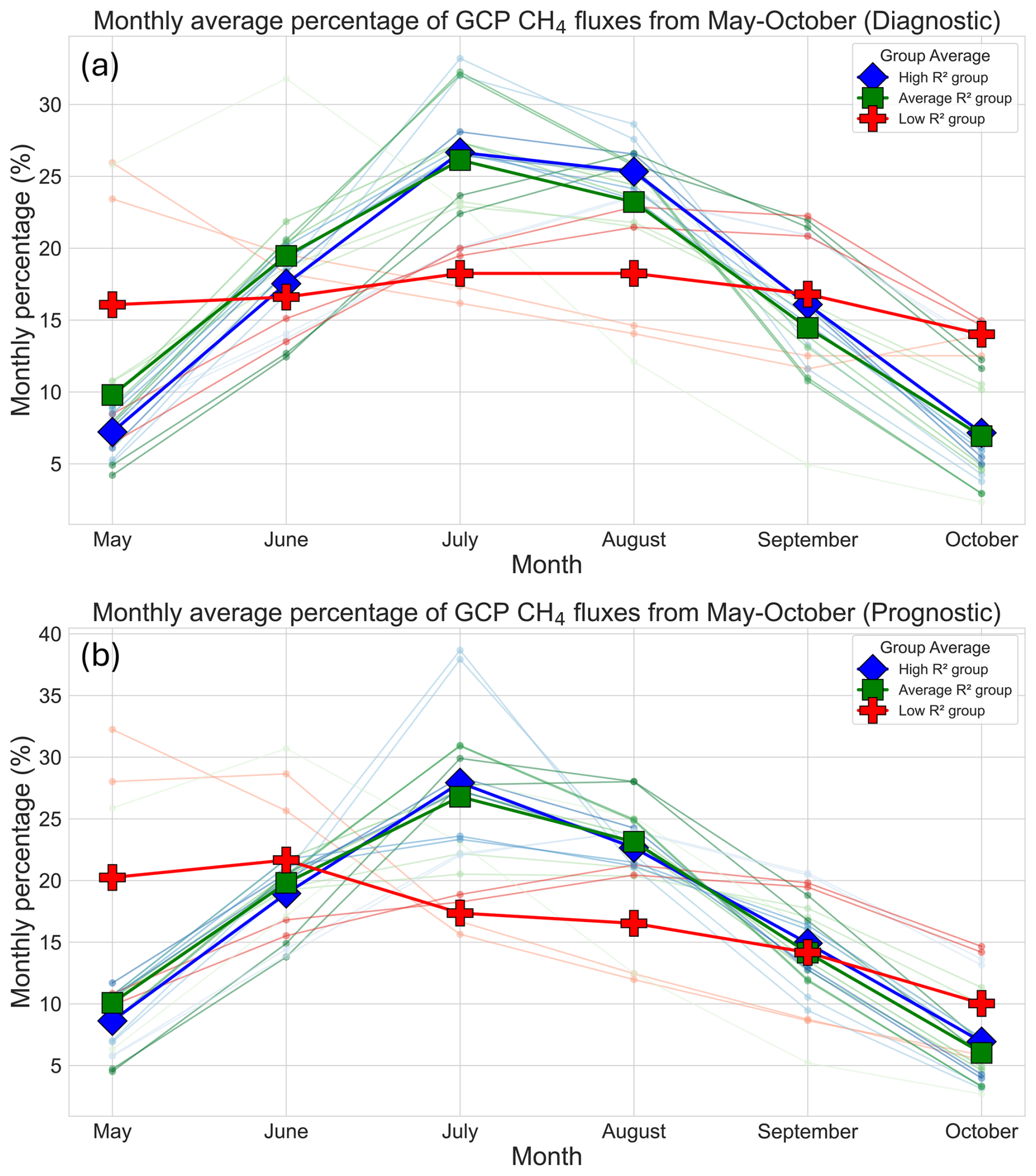
Figure 6 The seasonal cycles of the diagnostic GCP models (a) and prognostic GCP models (b) from 2007–2017. The blue, green, and red lines each represent the GCP models that have the highest, average, low R² values with atmospheric observations. The x axis represents the months from May to October throughout 2007–2017, and y axis denotes the percentages of CH₄ fluxes that occur within that month.

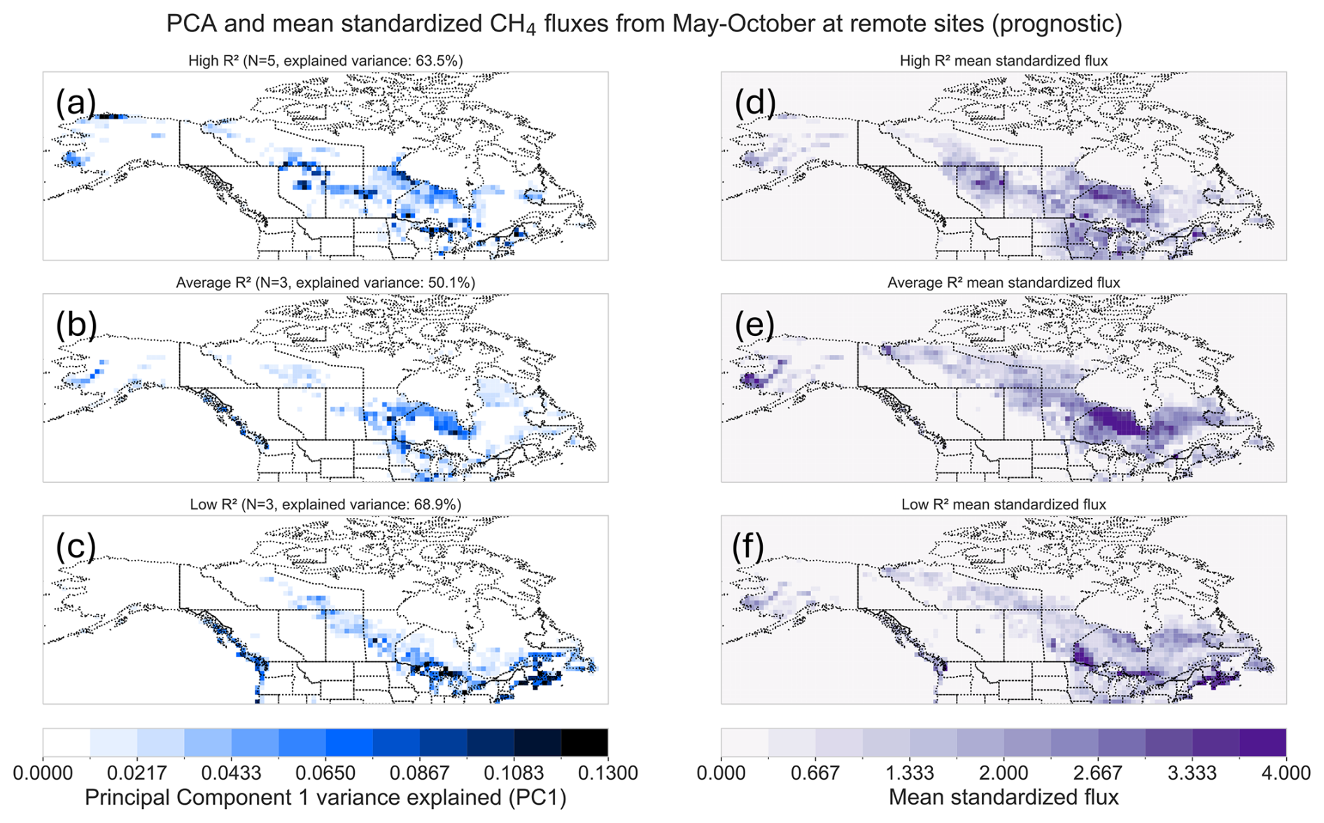
Figure 7 The PCA results and mean standardized CH₄ fluxes for the prognostic GCP models, run separately for each group of models – the high (a, d), average (b, e), and low (c, f) R² groups. The unit for PCA results is in explained variance by the first component (%), and darker (or more blue) shades represent better spatial agreements among the models within a same group.

Interestingly, we find that for 64 % ($\mathrm{7}/\mathrm{11}$) of the models, the diagnostic version of the model yields a better fit (R²) against atmospheric observations compared to the prognostic version of the model (Fig. 5. Prognostic versions of CLASSIC, SDGVM, LPX-Bern, and VISIT have better R² values compared to diagnostic versions). This result suggests that the better-performed diagnostic models may also reflect their reliance on a consistent inundation product, which potentially gives them the advantage in this evaluation framework over the more mechanistic prognostic models. In addition, process-based models with simpler and more deterministic formulations tend to produce smaller flux magnitudes and higher R² values compared to more complex models. This result indicates that simple formulations can effectively capture regional-to-continental flux patterns as those more complicated models (e.g., Miller et al., 2014, 2016b). However, more sophisticated process representations may become increasingly important for simulating finer-scale spatial structure or higher-frequency temporal variability of CH₄ fluxes.

We also find that the GCP models result in higher R² values and lower errors compared to the WETCHIMP models, both when comparing overlapping subsets of models and when considering their respective multi-model ensembles (Figs. S10 and S11). The ensemble of all WETCHIMP models yields a R² of 0.20 and an RMSE of 13.2 ppb. In contrast, the ensemble of all prognostic GCP models shows a R² of 0.35 with an RMSE of 11.9 ppb, while the ensemble of all diagnostic GCP models gives a R² of 0.39 with an RMSE of 11.5 ppb. These results demonstrate a clear improvement over the earlier WETCHIMP models, at least in comparisons with atmospheric observations.

3.4 Spatial distribution

We find that prognostic models that are most consistent with atmospheric observations concentrate their fluxes near the Hudson Bay Lowlands (Fig. 7a). In contrast, prognostic models with the lowest R² values focus their fluxes outside this key region (Fig. 7c). We focus this section on the prognostic models because the diagnostic models use the same inundation map and therefore exhibit similar spatial flux patterns. Similar to the previous analysis of seasonality, we group the prognostic models into three categories (high, average, low) depending on their R² values when compared against atmospheric observations. A Principal Component Analysis (PCA) highlights common spatial patterns among the models in each different group (e.g., Wold et al., 1987; Jolliffe, 1986; Delwiche et al., 2021). The percentage of variance explained by the first principal component (PC1) shows the degree of spatial patterns shared among models in each group, and this percentage captures how consistently the models agree in their spatial flux distributions across grid boxes within the study domain. We use the PC1 explained variance as a measure of within-group spatial coherence that quantifies how much of the between-model variance in a group is captured by a single grid. We find that models in the high R² group have a PC1 explaining 63.5 % of the variance, followed by the average R² group with 50.1 %, and the low R² group with 68.9 % explained variance. Although the low R² group shows the highest explained variance, this number does not necessarily indicate that the models in this group are more accurately capturing the true spatial patterns of the CH₄ fluxes compared to those in other groups.

We find notable common spatial features among the models in the high R², as seen in the PCA analysis. LPJ-wsl and CLASSIC have the highest R² values, and these models consistently concentrate their CH₄ fluxes in the Hudson Bay Lowlands. In contrast, JULES, ISAM, and ELM are the models with lower R² values. These models show large spatial discrepancies in critical wetland regions such as the Hudson Bay Lowlands, and they tend to concentrate fluxes outside of these key regions, particularly in the Great Lakes region of Canada.

An important caveat of this result is that the long-term observation network is sensitive to fluxes from some regions of high-latitude North America but not others (Fig. 1). The PCA analysis itself is unweighted, and our interpretation of spatial patterns (based on the R² metric) is necessarily influenced by regions with stronger observational coverage. We also note that none of the atmospheric observing towers are directly located in the Hudson Bay Lowlands, but the STILT footprints shown in Fig. 1 indicates that the network is sensitive to CH₄ fluxes from the broader region, allowing us to draw conclusions about the spatial distribution of fluxes in and around the Hudson Bay Lowlands.

4 Conclusions

This study highlights areas of convergence and disagreement among state-of-the-art process models of wetland CH₄ fluxes. We compare the estimates with atmospheric CH₄ observations between May and October in high-latitude North America. In the first section of the paper, we find that GCP models have a much smaller flux magnitude and lower inter-model uncertainty across North America compared to a previous model inter-comparison (WETCHIMP). The GCP models, when passed through an atmospheric transport model, are more consistent with atmospheric CH₄ observations compared to the WETCHIMP models, though we argue that the current GCP model ensemble is still too high across much of Canada and Alaska. In the second section of the study, we find that process-based CH₄ models that are most consistent with atmospheric observations based on our R² analysis exhibit the highest percentage of fluxes in July and August relative to other months and have a sharper seasonal cycle. These process-based models also concentrate their fluxes near the Hudson Bay Lowlands while less skilled models often concentrate fluxes further south near the Great Lakes.

Overall, we emphasize several opportunities to improve current process-based models of wetland CH₄ fluxes. Key areas for improvement include addressing (1) uncertainties in inundation or wetland extent and (2) improving estimated maps of soil carbon, though the latter factor was difficult to evaluate this study. We find that prognostic models show greater room for improvement than the diagnostic models because they show less agreement with atmospheric observations based on the R² and RMSE metrics. While diagnostic models benefit from consistent inundation maps, the development of better prognostic models is nevertheless very important because these models can be used to project future trends in wetland extent or inundation, which is critical for future projections of CH₄ fluxes under ongoing climate change. Overall, we argue that the bottom-up modeling community had made large strides in reducing inter-model uncertainties, and these improvements are consistent with atmospheric CH₄ observations based on our analysis using the STILT model. We note, however, that the GCP models are global and drivers vary regionally, so these conclusions apply only to our domain and time period. With that said, there is still an enormous need for further improvements in these models to advance understanding of high-latitude wetland CH₄ fluxes in a changing climate.