Model analysis of biases in the satellite-diagnosed aerosol effect on the cloud liquid water path

The response in cloud water content to changes in cloud condensation nuclei remains one of the major uncertainties in determining how aerosols can perturb cloud properties. In this study, we used an ensemble of large eddy simulations of marine stratocumulus clouds to investigate the correlation between cloud liquid water path (LWP) and the amount of cloud condensation nuclei. We compare this correlation directly from the model to the correlation derived using equations which are used to retrieve liquid water path from satellite observations. Our comparison shows that spatial variability in cloud properties and instrumental noise in satellite retrievals of cloud optical depth and cloud effective radii results in bias in the satellite-derived liquid water path. In-depth investigation of high-resolution model data shows that in large part of a cloud, the assumption of adiabaticity does not hold, which results in a similar bias in the LWP–CDNC (cloud droplet number concentration) relationship as seen in satellite data. In addition, our analysis shows a significant positive bias of between 18 % and 40 % in satellite-derived cloud droplet number concentration. However, for the individual ensemble members, the correlation between the cloud condensation nuclei and the mean of the liquid water path was very similar between the methods. This suggests that if cloud cases are carefully chosen for similar meteorological conditions and it is ensured that cloud condensation nuclei concentrations are well-defined, changes in liquid water can be confidently determined using satellite data.

1 Introduction

Clouds play a crucial role in the Earth's climate, affecting the radiative balance of the Earth as they cover the majority of the Earth's surface and have high reflectivity of the incoming solar radiation and absorbing outgoing thermal radiation (Bellouin et al., 2020; Forster et al., 2021). As aerosol can perturb the cloud properties, accurate knowledge of how aerosol–cloud interactions affect clouds will allow for better estimation on how changes in anthropogenic emissions affect the Earth's radiative balance and thus the climate. Satellite based estimates of aerosol effects on clouds have proven to be challenging to interpret as they have not always supported the theoretical assumptions of decreasing cloud droplet sizes with an increasing number of cloud droplets (Twomey, 1974; Jia et al., 2019) or the increase in cloud liquid water content with an increasing number of cloud droplets (Albrecht, 1989; Gryspeerdt et al., 2019). These mixed results have been attributed to several counteracting physical processes, for example the effects of solar heating, cloud-top mixing, and variability in moisture on the liquid water path (LWP) (Feingold et al., 2022; Gryspeerdt et al., 2022; Glassmeier et al., 2021; Zhang et al., 2024), but also challenges in satellite retrievals (Feingold et al., 2022; Arola et al., 2022).

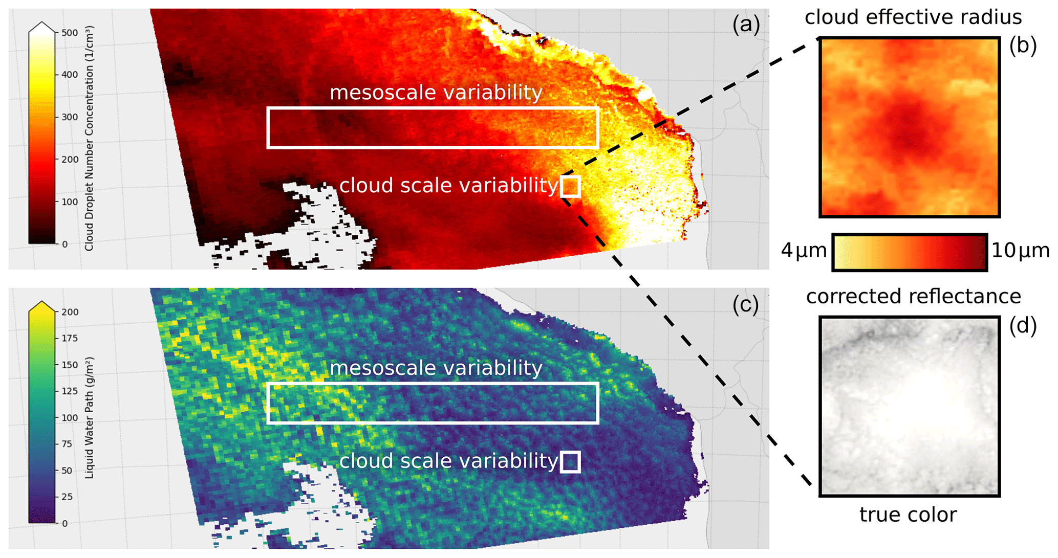
Figure 1 Cloud properties of a stratocumulus cloud deck west of Peru and Chile over the South Pacific on 30 August 2003. Panel (a) shows the CDNC calculated according to Quaas et al. (2006), and panel (c) shows the retrieved LWP from Moderate Resolution Imaging Spectroradiometer (MODIS) Level-2 (L2) Collection 6.1 (Platnick et al., 2015). Panels (b) and (d) show a magnification of the structure of a cloud cell within the cloud field, denoting the cloud effective radius and the cloud reflectance for the corresponding cloud cell. Small squares are approximately 3 km×3 km, and large rectangles are approx. 500 km×6 km.

Arola et al. (2022) showed that variability in positively correlated cloud droplet number concentration (CDNC) and liquid water path (LWP) data will dilute the correlation and can even result in an apparent strongly negative correlation between CDNC and LWP. However, in that study, the causes of variability were not studied further. Such variability can come from (1) internal variability in clouds originating from the circulation within clouds, e.g., in updrafts at the center of the cloud cells and downdrafts at the edges of the cell; (2) mesoscale variability in meteorological conditions and phase of the cloud evolution; and (3) instrumental noise in satellite retrievals.

Figure 1 shows the cloud properties in a stratocumulus deck west of Peru and Chile, South America. In the figure, the wide rectangles show regions in the cloud field, which show mesoscale variability in CDNC and LWP, while the small squares indicate internal variability in CDNC and LWP within a cloud cell. The smaller squares are magnified in the right-hand side panels, showing both the effective radius and the reflectivity of the cloud at visible wavelengths. The wide rectangle in the figure shows a region with significant mesoscale variabilities in cloud properties.

As for the small squares in Fig. 1, we can see that the retrieved cloud effective radius decreases towards the cloud cell edges. The decrease in retrieved cloud effective radius results from the entrainment mixing at the cloud top and downdrafts in the cloud cell boundaries, which both reduce the liquid water path. At the cloud cell edges, this is in conflict with the assumptions made in the calculation of CDNC. Calculation of CDNC based on the effective radius, and assuming constant sub-adiabaticity, would lead to overestimation in retrieved CDNC values compared to the real CDNC values at the cell boundaries (see Eq. 2 in Sect. 2). In addition to actual variability in physical properties of clouds, satellite retrievals include uncertainties and instrument noise, causing another potential source of bias in the satellite-derived correlation between CDNC and LWP. All these different sources of variability are potential causes for biasing the estimate of the aerosol effect on the LWP, as shown by Arola et al. (2022).

In this study we use a cloud-resolving large eddy simulation (LES) model to investigate the relative contribution of these sources of variability (cloud condensation nuclei, cloud structure, and noise in satellite retrievals) to the correlation between CDNC and LWP. We will analyze how the diagnosed response in LWP to perturbed aerosol concentrations differs when calculated with equations used in the satellite retrievals of LWP, compared to LWP diagnosed directly from the LES model.

2 Methods

2.1 Model description

We simulated the effect of aerosol concentration on cloud properties, especially the liquid water content, using the UCLALES-SALSA large eddy simulation model (Stevens et al., 2005; Kokkola et al., 2008; Tonttila et al., 2017; Ahola et al., 2020). In this model setup, UCLALES, which simulates the dynamics of the boundary layer, is coupled to the aerosol–cloud model SALSA, which simulates aerosol and cloud droplet microphysics. SALSA has a sectional description for aerosol particles, cloud and precipitation droplets, and ice crystals.

The model is built around UCLALES, a platform for idealized cloud simulations. The model resolves the turbulent flow in a three-dimensional Cartesian grid with cyclic boundary conditions. The main prognostic scalar variables include the liquid water potential temperature and tracer variables describing water vapor and liquid water mixing ratios. When coupled with the sectional aerosol–cloud microphysics model SALSA, the set of prognostic scalars is vastly extended, now including the number and mass mixing ratios for each size section of four particle categories, comprising aerosol particles, cloud droplets, drizzle/precipitation, and ice (the latter not used in this study). The size-resolved framework is used to describe particle growth via condensation and coalescence processes in all categories. Aerosol cloud activation is determined directly from the resolved particle growth, whereas the transition between cloud droplets and drizzle is diagnosed from the resolved collision–coalescence process. UCLALES-SALSA has been validated against observations in liquid phase clouds and fogs and found to reproduce the observed droplet distributions (e.g., Boutle et al., 2018; Calderón et al., 2022). More details on the model and simulations are given in Sects. S1 and S2 in the Supplement.

2.1.1 Experiment setup

To better understand the features of the LWP response to changes in CDNC seen in the satellite data, UCLALES-SALSA was configured for a typical marine stratocumulus cloud setup (nocturnal drizzling stratocumulus cloud DYCOMS-II RF02 of the Second Dynamics and Chemistry of Marine Stratocumulus field campaign, Ackerman et al., 2009), representing a very commonly occurring cloud type, which allows for disentangling the potential underlying numerical biases related to satellite retrievals. The horizontal model domain size was 51×51 km with a resolution of 75 m, with the vertical domain extending up to 1.4 km and a vertical resolution of 20 m. Vertical profiles of atmospheric variables used for model initialization are shown in Fig. S1 in the Supplement.

For aerosol, we used a bi-modal size distribution. The Aitken mode is centered at 0.022 µm, with a standard deviation of 1.2 and a total number concentration of 150 cm⁻³. The accumulation mode is centered at 0.120 µm, with a standard deviation of 1.7. To determine the effect of aerosol on cloud properties, we ran a set of three simulations with cloud condensation nuclei (CCN) equivalent to initial accumulation-mode aerosol concentrations of 65, 150, and 300 cm⁻³ (corresponding to the total number concentrations of 78, 180, and 360 cm⁻³ for the whole size distribution). Size distributions are illustrated in Fig. S2 in the Supplement.

The simulations span 14 h, and the model output was sampled 2, 6, and 10 h from the start of the run. These time intervals allow us to draw samples from different cloud structures, as the microphysical properties and circulation structures are allowed to evolve freely in the model. In particular, the simulations with the lowest initial aerosol concentrations exhibit a clear drizzle-induced transition from closed stratocumulus cells to an open-cell structure within 10 h of model time.

It is well-known that satellite-based CDNC values are biased because radiances used in the cloud effective radius (CER) retrievals correspond to an optically thicker region below the cloud top. Platnick (2000) established that infrared radiance fluxes from liquid clouds include all reflected photons that penetrate to a maximum optical depth equivalent to up to 3.5 units below the cloud top (Grosvenor et al., 2018b) depending on the viewing geometry and cloud heterogeneity (Grosvenor et al., 2018a). With CER values that are smaller than those expected at the cloud top, the cloud-top-based pseudo-adiabatic model inevitably fails, producing satellite retrievals of CDNC and LWP that are different from real ones (Grosvenor et al., 2018a).

In this study, we followed a sampling methodology that mimics this so-called penetration depth bias (Grosvenor et al., 2018a). We determined the CER and CDNC values for the top part of a cloud based on as many model layers as needed to reduce the cloud optical thickness (COT) in the infrared region by three units. The infrared COT was calculated using the wavelength band of 2.38–4.00 µm to match the MODIS retrievals done at the 2.13 and 3.7 µm channels. Both CER and CDNC were calculated as average values weighted by the extinction coefficient b_ext that consider all model layers in the top part of the cloud (Eqs. S.1 and S.2). For the sake of simplicity we refer to this region as the extended cloud top. COT was calculated for the visible wavelength band of 0.25–0.69 µm as a surrogate of MODIS retrievals done at 0.66 µm. More details on the sampling methodology can be found in Sect. S2 in the Supplement.

Values for CDNC (N_d) were calculated with CER (r_e) and COT (τ_c) obtained for the extended cloud top in each cloud column from the following equation:

$$\begin{array}{}\text{(1)}& N_{\mathrm{d}}={\displaystyle \frac{\sqrt{\mathrm{5}}}{\mathrm{2}\mathit{\pi }k}}{\left({\displaystyle \frac{f_{\mathrm{ad}}{c}_{\mathrm{w}}{\mathit{\tau }}_{\mathrm{c}}}{Q_{\mathrm{ext}}{\mathit{\rho }}_{\mathrm{w}}{r}_{\mathrm{e}}^{\mathrm{5}}}}\right)}^{\frac{\mathrm{1}}{\mathrm{2}}},\end{array}$$

where k is the relation of volume mean radius and effective radius of the droplet size distribution, f_ad is the adiabaticity factor, c_w is the rate of increase of liquid water content with height in a moist adiabatically ascending air parcel, Q_ext is the Mie extinction efficiency, and ρ_w is the density of water (Grosvenor et al., 2018b). The parameters k, f_ad, c_w, Q_ext, τ_c, and r_e were diagnosed from the UCLALES-SALSA model.

The cloud parameters k, f_ad, c_w, and Q_ext vary with time along the cloud structure. However the actual values cannot be directly derived from MODIS observations, and thus they are assumed to be constant and denoted by α, for which an often-used value for marine stratiform clouds is $\mathrm{1.37}\times {\mathrm{10}}^{-\mathrm{5}}{\mathrm{m}}^{-\frac{\mathrm{1}}{\mathrm{2}}}$ (Quaas et al., 2006; Grosvenor et al., 2018b; Gryspeerdt et al., 2022; Arola et al., 2022). Estimates of f_ad could possibly be improved by combining MODIS and CALIOP observations. Consequently, CDNC values can be obtained from

$$\begin{array}{}\text{(2)}& N_{\mathrm{d}}=\mathit{\alpha }{\mathit{\tau }}_{\mathrm{c}}^{\frac{\mathrm{1}}{\mathrm{2}}}{r}_{\mathrm{e}}^{-\frac{\mathrm{5}}{\mathrm{2}}}.\end{array}$$

LWP values were calculated with the following equation (Wood, 2006):

$$\begin{array}{}\text{(3)}& \mathrm{LWP}=\mathrm{5}/\mathrm{9}{\mathit{\rho }}_w{r}_{\mathrm{e}}{\mathit{\tau }}_{\mathrm{c}}.\end{array}$$

In the analysis, we filtered the data so that we only considered cloudy columns where τ>4 and $\mathrm{4}\mathrm{\mu }\mathrm{m}<r_{\mathrm{e}}<\mathrm{15}\mathrm{\mu }\mathrm{m}$, similar to Gryspeerdt et al. (2019) and Arola et al. (2022). An example of cloud field properties can be seen in Fig. S3.

2.2 Results

2.2.1 The effect of cloud internal variability on retrieved CDNC and LWP

First, to get an indication on how the cloud cell level variability affects the satellite-retrieved LWP adjustment, we compared model-predicted CDNC and LWP values with CDNC and LWP values calculated using Eqs. (1)–(3). We carried out an ensemble of UCLALES-SALSA simulations, varying the conditions for cloud formation and the number concentrations of aerosol particles, and then analyzed the simulated CDNC and LWP values with the approaches detailed below.

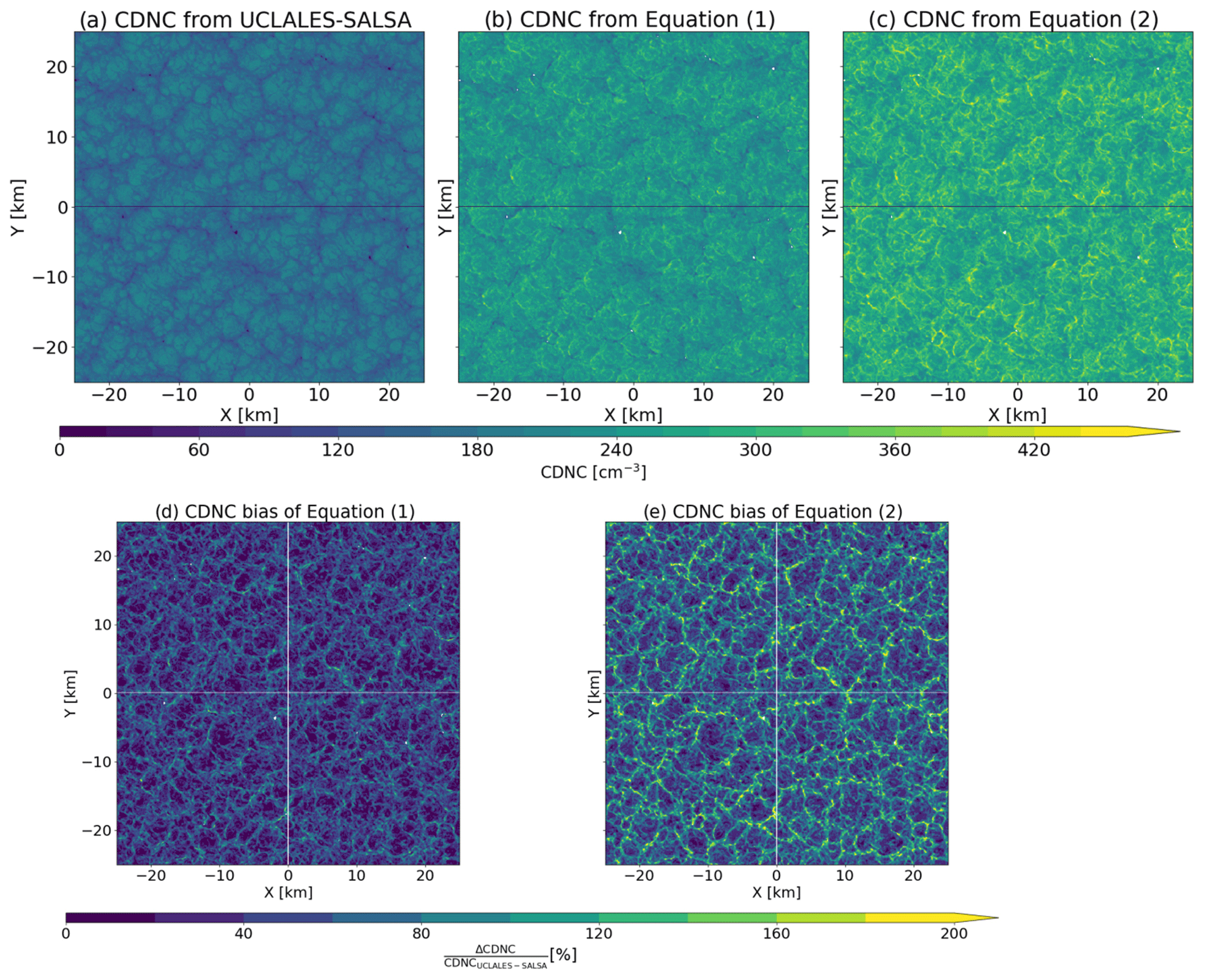
Figure 2 CDNC at the cloud top (a) from the direct output of UCLALES-SALSA, (b) calculated using Eq. (1) with UCLALES-SALSA-simulated values for all parameters, (c) using Eq. (2), (d) relative biases in CDNC between UCLALES-SALSA and Eq. (1), and (e) relative biases in CDNC between UCLALES-SALSA and Eq. (2).

As an example, Fig. 2 shows the cloud droplet number concentration over the model domain of a simulation where the model was initialized with a total aerosol number concentration of 300 cm⁻³. The leftmost panel in Fig. 2 represents CDNC values diagnosed directly from the UCLALES-SALSA model. In the middle panel, CDNC was calculated from Eq. (1), using LES-simulated values for k, f_ad, c_w, Q_ext, τ_c, and r_e in the equation. In the rightmost panel CDNC was calculated from Eq. (2), assuming constant α of $\mathrm{1.37}\times {\mathrm{10}}^{-\mathrm{5}}{\mathrm{m}}^{-\frac{\mathrm{1}}{\mathrm{2}}}$ and using simulated τ_c and r_e.

The leftmost panel shows a closed-cell-type structure in the cloud, with lower values for CDNC at the boundaries of the cells. A snapshot of LWP is shown in the Supplement, Fig. S3. Note that the simulated cloud in Fig. 2 is fully overcast, also at the cloud cell edges. Comparing Fig. 2a and b, we can see that when all the parameters in Eq. (1) are from LESs, CDNC corresponds quite well with the model values, showing a similar structure although overestimating the CDNC throughout the model domain. However, the averaging of satellite data will mitigate this since spatial aggregation of the data will reduce the maximum CDNC values (see the differences between Figs. S9 and S10 in the Supplement) making the CDNC distribution more narrow (Fig. S11). This is also in line with observations where aircraft- and satellite-observed CDNC is compared (Gryspeerdt et al., 2022).

Comparing Fig. 2a and c, we can see that when we use a fixed value for α, the satellite equation exhibits inverse behavior at cloud cell boundaries compared to the direct output of the model; i.e., CDNC increases towards the boundaries of the cloud cells. This indicates that the assumptions of, e.g., adiabaticity do not hold at the cloud cell boundaries. This is also in line with a previous study by Feingold et al. (2022). Biases in LWP also occur differently across cloudy areas (Fig. S5). Cloud cell boundaries tend to have low biased LWP values, while cloud cell centers are biased high. In cloud cell boundaries, processes such as entrainment and lateral mixing lead to sub-adiabaticity. Since these sources of variability are not considered in the formulation of satellite retrieval equations, there are important deviations from the assumptions of vertically constant values for droplet number concentration, droplet size distribution breadth, and adiabaticity. A more detailed analysis of CDNC biases related to changes in LWP, cloud effective radius, and the adiabatic factor has been included in Fig. S15.

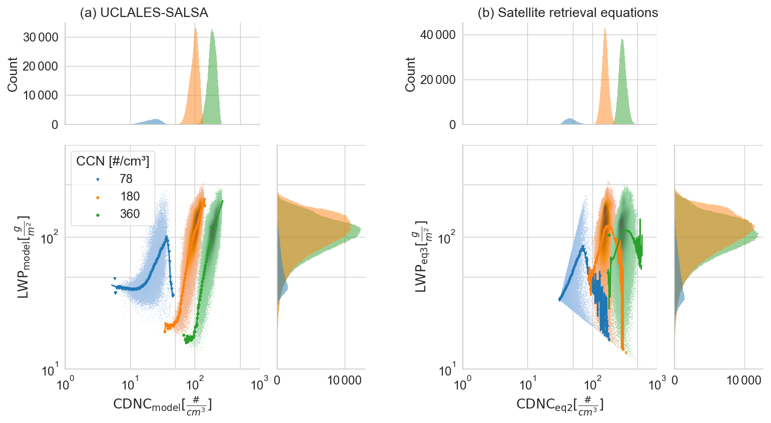
Figure 3 Joint and marginal histograms for LWP and CDNC values using (a) UCLALES-SALSA and (b) Eq. (2) at a time instance of 6 h. Simulations are color-coded according to CCN concentrations used in the model initialization. The intensity of color in joint histograms increases when the probability increases. The probability is represented as a density function calculated as counts$/$sum(counts)$/$bin area. Continuous lines indicate the arithmetic mean.

To see how the discrepancy between the cloud properties diagnosed directly from UCLALES-SALSA and using Eq. (3) translates to differences in the correlation between CDNC and LWP, we calculated this relation for all ensemble members. Figure 3 illustrates LWP as a function of CDNC for direct model input and calculated using Eqs. (2) and (3) for the three different initial CCN concentrations at 6 h into the simulation. For all initial CCN concentrations, the direct model output indicates an almost linear correlation in the log–log scale within single cloud scenes. For an individual simulation, the positive slope between CDNC and LWP reflects the horizontal structure of the cell, where air flows from the core, characterized by high LWP and high CDNC, outward toward the cell edges with lower LWP and CDNC. The lowest CCN case exhibits a drop in LWP at highest CDNC values. However, the number of data points is very low at highest CDNC values. In contrast, when using Eqs. (2) and (3) the variability and the unphysical behavior in N_d at the boundaries of cloud cells yield curves which reach a local maximum, and for higher CDNC values they exhibit a downward slope with increasing CDNC. In addition, CDNC values have a clear high bias. In this case, satellite-derived CDNC values are at least 2 times higher than the direct LES values. Values are positively biased due to the assumption of vertically uniform cloud columns which is not valid in thin cloud layers such as those observed at cloud cell edges. Although the spatial resolution in LES is much higher than in satellite data and it has been shown that spatial and temporal averaging affects the CCN–LWP correlation (Rosenfeld et al., 2023), this behavior is similar to what is seen in satellite data and what was also demonstrated with synthetic data by Arola et al. (2022). This same behavior was seen in all of the ensemble members over all analyzed time instances and all CCN concentrations (Figs. S6–S8).

The probability distributions of CDNC and LWP data are shown at the top and to the right of the coordinate frame, respectively, in Fig. 3. From these distributions we can see that LES-derived data are skewed towards higher CDNC values, while the LWP probability distributions look very similar for both LES and satellite equations. The sharp cutoff of data at low LWP and CDNC values is caused by filtering of the data to include only values where τ>4 and $\mathrm{4}\mathrm{\mu }\mathrm{m}<r_{\mathrm{e}}<\mathrm{15}\mathrm{\mu }\mathrm{m}$. Earlier studies on satellite data limit this filtering to CDNC but not to LWP (Gryspeerdt et al., 2019). However, due to doing pixel-by-pixel analysis for CDNC–LWP correlation, both CDNC and LWP data are filtered here.

Within individual ensemble members, the cloud internal variability contributes to the CDNC–LWP correlation and cannot be considered to be an aerosol effect on clouds, also shown by Zhou and Feingold (2023). In addition, in the analysis of satellite data, it is a common practice to avoid non-adiabatic clouds (e.g., Grosvenor et al., 2018b), so that issues in satellite-retrieved cloud properties at, for example, cloud cell edges can be avoided. Previous studies have shown that selecting adiabatic pixels in a model and satellite analysis brings their results closer to each other (Dipu et al., 2022). Varble et al. (2023) also showed that removing the differences between the adiabaticity in an Earth system model and satellite retrievals brings the observed and satellite-retrieved LWP adjustment closer to each other.

2.2.2 The effect of combining different aerosol and time instances on CCN–LWP correlation

In addition to internal variability within clouds due to the dynamics affecting the cloud structure, cloud scenes can include clouds at different phases, e.g., transitioning between a closed-cell structure and an open-cell structure. Cloud scenes can also include large-scale variability in the cloud geometric thickness and water content, which is due to differences in meteorological conditions rather than caused by differences in aerosol concentration. To get an indication on how such variability affects the correlation between LWP and CDNC, we analyzed simulated cloud scenes at different points in time (2, 6, and 10 h). During the simulation, the closed-cell structure transformed to an open-cell structure for the case with the lowest initial aerosol load, and for the cases of higher aerosol load, the size of convective cells increased.

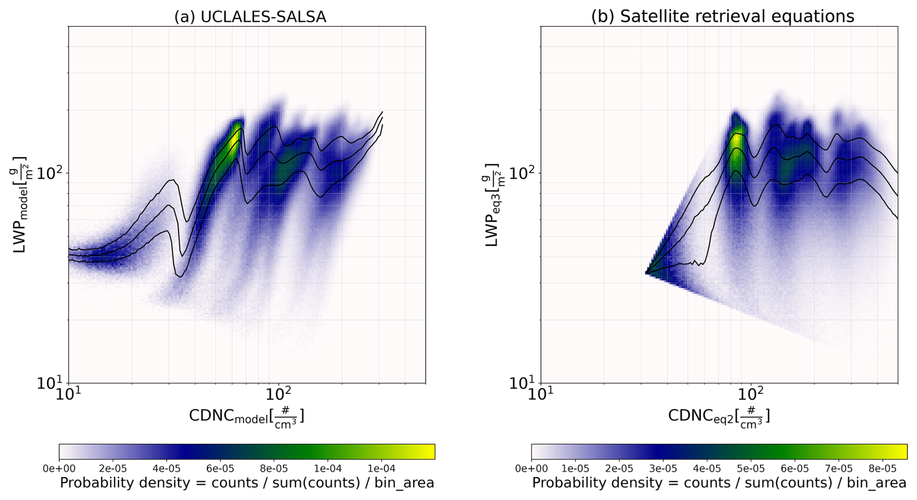
Figure 4 Joint histogram of LWP as a function of CDNC (a) from the direct output of UCLALES-SALSA, (b) calculated using Eqs. (2) and (3) assuming a constant α. Black continuous lines indicate the 25th, 50th, and 75th percentiles of LWP per bin. The color scale indicate the probability density calculated as counts$/$sum(counts)$/$bin area.

Figure 4 shows the correlation between CDNC and LWP from direct model output and calculated using Eqs. (2) and (3) when all the cloud scenes are aggregated. Figure 4a shows that the model produces an overall positive correlation, while satellite equations produce a similar shape correlation as shown in Fig. 3b for one ensemble member, only spreading over a wider CDNC range due to the variability in CDNC concentrations. The direct model output resembles the shape of the correlation between CDNC and LWP simulated by the ICON model in Fons et al. (2024), while the satellite equation exhibits a decrease in LWP at CDNC values higher than 300 cm⁻³.

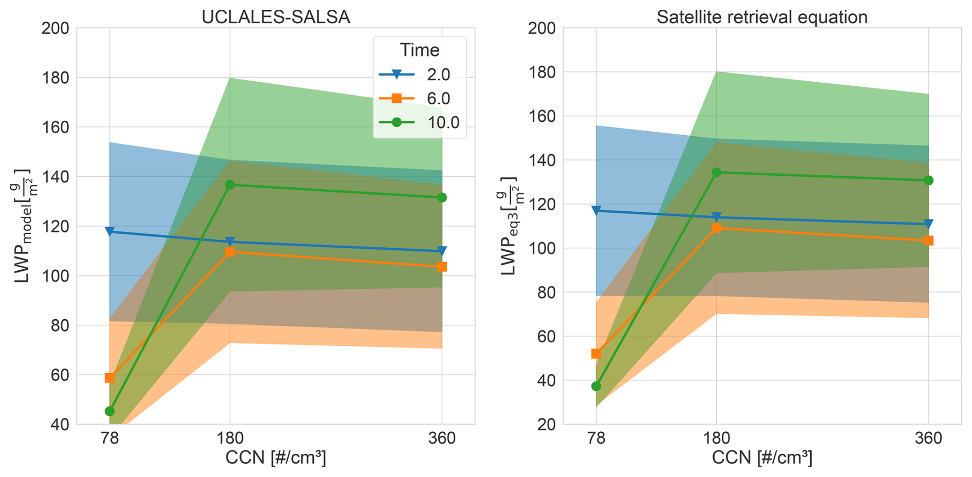
To further investigate the differences between the LES model and satellite equations, we compared the mean LWPs of the LES domain using both direct output and satellite-equation-derived LWP for different initial aerosol concentrations. Figure 5 represents a proxy for satellite aggregation. It shows the LES domain mean LWP at three different time instances into the simulation for three different runs as a function of the initial CCN concentration. Solid lines denote the mean LWP in the domain, and the shading indicates the standard deviation in the data.

Early into the simulation, we expect the simulated clouds to be close to a very similar phase of the cloud cycle, and thus the difference in LWP between the different aerosol cases comes mainly from the differences in CCN concentrations. During the first 2 h into the simulation there has not been enough time for precipitation to develop, and thus the LWP decreases slightly as a function of CCN concentration. Previous LES studies of the same DYCOMS case have produced qualitatively similar results (Ackerman et al., 2009; Bulatovic et al., 2019). Later in the simulation, precipitation is initiated with the lowest CCN concentration, and a typical shape of CCN–LWP correlation is reached where LWP first increases with CCN and then decreases due to increased entrainment rate (Ackerman et al., 2009; Bulatovic et al., 2019). However, the difference in LWP between CCN concentrations of 180 and 360 cm⁻³ does not change significantly from 6 to 10 h into the simulation, which is opposite to the findings in Glassmeier et al. (2021) and can be characteristic of the DYCOMS2 input profile with quite a small moisture inversion. The figure also illustrates that although we also included non-adiabatic model grid points in calculations where Eqs. (2) and (3) are used, changes in LWP with increasing CCN are strikingly similar to those diagnosed from the LES model. There is a slight bias in satellite-equation-derived LWP (Fig. S5) in all the cases, but the relative changes correspond well with LES-diagnosed relative changes in LWP. This indicates that if cloud condensation nuclei concentrations are well-defined, changes in liquid water path due to changes in aerosol can be confidently determined using satellite data.

This analysis indicates that, when using domain-averaged CCN and LWP values, the non-adiabaticity of the cloud cell edges does not contribute significantly to the correlation between CDNC and LWP with an “inverted v” shape, seen in satellite data. Although there are issues in using Eqs. (2)–(3), coarse resolution of satellite data will reduce these issues significantly. Due to their coarse resolution, satellite data can include both cloud cell centers and edges and could, therefore, introduce bias in the retrieved LWP values. However, based on Fig. 5, in our simulated cases this aggregation of different cloud structures does not affect the derived response in LWP to changes in CCN. We also tested this using spatial averaging of 1.425 km by 1.425 km to correspond to the spatial resolution of satellite data. Since radiances are directly proportional to cloud optical thickness, we use COT values in cloudy columns as a weighting factor to perform horizontal averaging operations along subdomains. Figures S9 and S10 in the Supplement illustrate that spatially averaged data shows very similar cloud field properties with less frequent large CDNC relative deviations because averaging reduces the variability in r_e (Fig. S11). The CCN–LWP-shaped correlation for different time instances and CCN scenarios lacks the inverted v shape (Figs. S12, S13, and S14).

Figure 5 LWP as a function of CCN from the direct output of UCLALES-SALSA and calculated using Eq. (3). Time instances are color-coded. Shaded areas indicate the spread of values in terms of the standard deviation.

2.2.3 The effect of satellite instrument uncertainty or variability on retrieved CDNC and LWP

In addition to variability in cloud properties that originate from variability in aerosol concentrations and meteorological conditions, satellite instruments also include uncertainty, originating from instrument noise as well as three-dimensional radiative effects. Such variability or noise will further affect the correlation between CDNC and LWP. Here we repeated the analysis combining all analyzed cases and adding 20 % variability in both τ_c and r_e and then calculating CDNC and LWP from Eqs. (2) and (3). The level of variability was chosen to be in line with that used in Arola et al. (2022).

Figure 6 shows that adding noise produces a CCN–LWP correlation that increases, reaches a local maximum, and then decreases. However, the additional noise does not affect the correlation between CDNC and LWP compared to Fig. 4b. Both Figs. 3b and 4b exhibit a similar “inverted v” behavior of the same magnitude. At high CDNC values the negative correlation becomes less pronounced due to the variability in x scale, i.e., increased variability in CDNC.

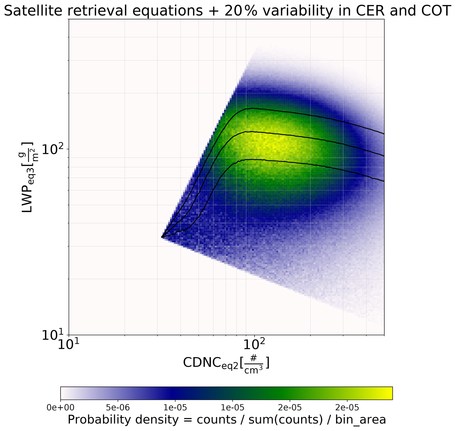
Figure 6 Joint histogram of LWP as a function of CDNC calculated using Eqs. (2) and (3) assuming a constant α and including 20 % variability in τ_c and r_e. Black continuous lines indicate the 25th, 50th, and 75th percentiles of LWP per bin. The color scale indicates the probability density calculated as counts$/$sum(counts)$/$bin area.

3 Conclusions

Our LESs show that variability in cloud properties when including different cloud types, CCN concentrations, and clouds in different phases of their cycle will bias satellite-derived correlation between CDNC and LWP, similar to Arola et al. (2022). The root cause for this is that variability in the cloud effective radius causes stronger positive bias in cloud droplet number concentration when using the retrieval equation (Eq. 2). Although our LESs include a detailed description of aerosol–cloud interactions, they do not consider the following potential error sources: 3D radiative effects in broken cloud fields, viewing geometry effects on the penetration depth bias, cloud heterogeneity at regional scale, and changes in surface reflectivity induced by changes in cloud coverage (Grosvenor et al., 2018a). Nonetheless, we could not find evidence in our model results to validate the persistent negative LWP adjustment predicted by satellite equations for stratocumulus clouds affected by aerosol perturbations.

Cloud cell level variability in cloud effective radius and cloud optical thickness caused a significantly different response in LWP with respect to changes in CDNC within individual simulations with different aerosol loads. However, when comparing the direct output of LWP from LES and that derived using Eq. (3) for different CCN values, both show a remarkably similar response between CCN and LWP. This indicates that although the adiabaticity assumption near cloud edges causes error in CDNC and LWP, on average, equation-derived LWP (Eq. 3) corresponds well with averaged LWP diagnosed from the LES output (see Fig. 5). Furthermore, the relatively coarse resolution of satellite retrievals mitigates the impact of cloud cell level variability through averaging. However, CDNC is overestimated when using Eq. (2), especially at lower LWP values, and this highlights the need to obtain a good constraint for CCN instead of using satellite-derived CDNC as a proxy for CCN. Based on this, determining LWP requires careful selection of clouds, estimating the mean LWP for different aerosol loads, e.g., over regions where there has been a clear change in aerosol emissions. Since this study focuses only on one cloud case, analysis could be extended to cover wider variability in cloud conditions using, for example, large-scale aerosol-aware high-resolution climate models, which would also capture the mesoscale variability. The “inverted v” shape functionality of LWP adjustments is seen in simulations of general circulation models (GCMs) of the current generation and could be introducing confounding effects into the effective radiative forcing of aerosol–cloud interactions (ERFaci) (Mülmenstädt et al., 2024). This clearly highlights that the behavior of cloud water in response to changes in aerosol remains an open question, and current knowledge does not support modifying the climate model cloud schemes to produce the “inverted v” behavior.