Finite domains cause bias in measured and modeled distributions of cloud sizes

A significant uncertainty in assessments of the role of clouds in climate is the characterization of the full distribution of their sizes. Order-of-magnitude disagreements exist among observations of key distribution parameters, particularly power law exponents and the range over which they apply. A study by Savre and Craig (2023) suggested that the discrepancies are due in large part to inaccurate fitting methods: they recommended the use of a maximum likelihood estimation technique rather than a linear regression to a logarithmically transformed histogram of cloud sizes. Here, we counter that linear regression is both simpler and equally accurate, provided the simple precaution is followed that bins containing fewer than ∼ 24 counts are omitted from the regression. A much more significant and underappreciated source of error is how to treat clouds that are truncated by the edges of unavoidably finite measurement domains. We offer a simple computational procedure to identify and correct for domain size effects, with potential application to any geometric size distribution of objects, whether physical, ecological, social or mathematical.

1 Introduction

The broad range of cloud sizes in the atmosphere poses a significant challenge to the modeling of weather and climate. Small clouds tend to be most numerous, while large clouds have more significant meteorological and climate impacts. An approximate balance means that all size classes contribute to overall cloud cover (Wood and Field, 2011), total rainfall (Peters et al., 2009) and the dissipation of buoyant potential energy (Garrett et al., 2018). The commonly used “divide-and-conquer” approach to the problem isolates a particular spatial scale for study, such as mesoscale convective systems larger than ∼ 100 km (Houze, 2004), shallow clouds in the trades between 20 and 200 km (Stevens et al., 2020; Bony et al., 2020) or sub-kilometer cumulus (Koren et al., 2008; Mieslinger et al., 2019). While this approach has practical benefits, it cannot easily be used to address how clouds of all scales interact.

Revealingly, independent of the spatial scale or cloud type considered, the measured horizontal dimensions of clouds tend to follow power law distributions such that the number of clouds is proportional to their size to some power (Cahalan and Joseph, 1989; Wood and Field, 2011; Mieslinger et al., 2019; Savre and Craig, 2023). Quantities that follow power law distributions are often described as being “scale-free” or “scale-invariant”, meaning that there is no “characteristic” object scale as there would be in defining, e.g., an exponential or Gaussian distribution. Power law behavior is in fact quite general among physical, social and biological systems, applying to, e.g., meteor diameters, neuronal firing, personal incomes, city populations and forest sizes (Buzsáki and Draguhn, 2004; Newman, 2005; Bettencourt et al., 2007; Saravia et al., 2018).

Quantities that exhibit scale-free behaviors, however deterministically complicated they may be, allow for an important mathematical simplification. That is, phenomena measured at any one scale shed light on the behavior at others. They also present a practical challenge, which is the unavoidable limitation that geometrically defined objects must inevitably be measured within a domain of some finite size, i.e., a domain that is not scale-free. The domain enforces a maximum scale for object measurement – the size of the domain – and this may not reflect the maximum scale that the objects can attain.

For cloud areas a, we recently argued that improper consideration of the scale of the measurement domain has contributed to wide discrepancies in the reported nature of cloud area distributions and in particular to the upper bound a_max to which a power law can be claimed to apply (DeWitt et al., 2024). Because clouds cannot be arbitrarily small, there must also be a lower bound a_min to the power law regime, one that has not yet been determined but that could approach the Kolmogorov microscale of ∼ 1 mm, below which turbulent circulations are damped by viscous forces. Between a_min and a_max, the power law regime can be represented by the probability distribution

$$\begin{array}{}\text{(1)}& n\left(a\right)\propto a^{-\left(\mathit{\alpha }+\mathrm{1}\right)};a_{min}<a<a_{max},\end{array}$$

where α is a constant, indicating that n(a) is linear on doubly logarithmic axes. The upper bound at a_max represents a “scale break” beyond which studies generally find that the distribution is “cut off” by a regime following either a steeper power law with a larger value of α or an exponential (Cahalan and Joseph, 1989; Benner and Curry, 1998; Neggers et al., 2003; Peters et al., 2009; Mieslinger et al., 2019; van Laar et al., 2019; Christensen and Driver, 2021; Savre and Craig, 2023).

Estimates of the location of the scale break at a_max differ widely. This uncertainty has underappreciated implications for studies of the role of clouds in climate because the integral ${\int }_{a_{min}}^{a_{max}}an\left(a\right)\text{d}a$, which is the total cloud amount, is sensitive to the scale break location. For example, a cutoff regime at areas of order ∼ 10 km², as suggested by some (Cahalan and Joseph, 1989; Benner and Curry, 1998; Neggers et al., 2003; Savre and Craig, 2023), would imply that clouds larger than ∼ 4000 km² would be so rare that they would contribute negligibly to the total, while other findings suggest that such large clouds contribute approximately 50 % to the global cloud cover (Wood and Field, 2011; DeWitt et al., 2024).

The power law exponent α for cloud areas is also highly uncertain, with similar implications for the relative roles of different cloud types. The exponent determines the relative numbers of small and large clouds. Values close to unity (e.g., Peters et al., 2009; Wood and Field, 2011; Mieslinger et al., 2019; DeWitt et al., 2024) imply that clouds of all orders of magnitude contribute equally to the total cloud cover, in which case small clouds that are often left unresolved by models and measurements may be an important omission. Conversely, values less than unity (e.g., Cahalan and Joseph, 1989; Benner and Curry, 1998; Neggers et al., 2003; Koren et al., 2008; Yamaguchi and Feingold, 2013; Bley et al., 2017; Senf et al., 2018; van Laar et al., 2019; Savre and Craig, 2023) indicate that large clouds dominate the total area and so remain a reasonable subject for more focused study.

The lack of consensus among studies on the value of α may be due to differences in the dominant cloud type that was considered or how diurnal variability affects a_max (van Laar et al., 2019). However, even if temporal and spatial variability of the size distribution exists, there remains a necessary prerequisite to measuring such variability, which is to first ensure that the size distribution is being accurately measured in the first place. To this end, Savre and Craig (2023) recently argued that, while size distributions do show some variability, the use of inaccurate statistical methods to fit power law distributions could also partially explain the lack of consensus among prior measurements of cloud sizes. In particular, they showed that the common method of fitting a least-squares linear regression to a logarithmically transformed histogram of cloud areas can lead to biased measurements of α.

Here we argue that the choice of fitting method is less important than whether past studies properly accounted for the finite size of the study domain. A finite domain size is a general problem for measuring scale-free quantities. For example, Serafino et al. (2021) argued that scaling properties of networks can be obscured by such finite-size effects, causing a truly scale-free network to appear non-scaling.

Similarly, cloud sizes must necessarily be measured within a non-scaling finite domain. It is easy to appreciate that the area of clouds larger than the domain size cannot be measured. A more subtle effect is that the measured numbers of clouds of a given area, even those smaller than the domain area, are highly sensitive to whether clouds that cross the domain edge are included or removed in the measured distribution (an example is shown in Fig. 1). We term such clouds “truncated clouds” as they appear effectively truncated by the domain edge, with only the portion of the cloud lying within the domain available for measurement.

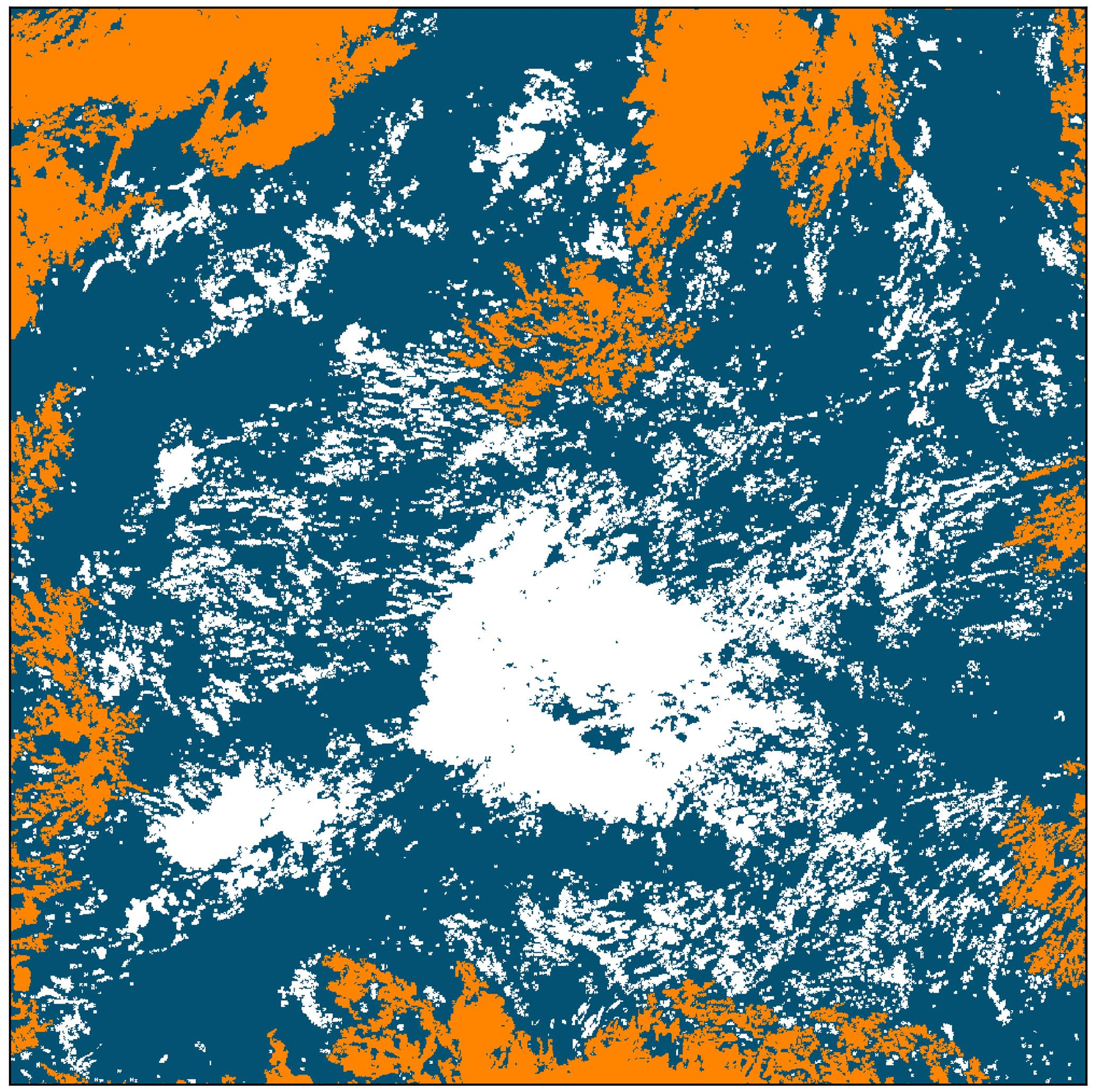
Figure 1 An example cloud mask derived from GOES satellite imagery, where cloudy pixels are white or orange and clear pixels are dark blue. Clouds which are truncated by the domain edge are marked in orange. The areas of such “truncated clouds” cannot be properly quantified as some unknown portion lies beyond the measurement domain.

Whether truncated clouds are included or removed from distribution fits is an issue rarely mentioned in past studies, but those that do consider the effect tend to remove truncated clouds without applying any correction factor (e.g., Peters et al., 2009; Christensen and Driver, 2021). One exception is a study of one-dimensional cloud chords by Wood and Field (2011), who found that the removal of chords truncated by the domain edge leads to an undercounting of large chords relative to what would be measured in a larger domain. For cloud areas, it may be hypothesized that a similar effect could explain the observed differences in measurements of a_max.

In this study, Sect. 2 reconsiders the hypothesis proposed by Savre and Craig (2023) that discrepancies in distribution parameters can be largely explained by improper methods used to fit a power law distribution to measurements of cloud sizes. Section 3 then examines how the choice of either including or removing clouds that are truncated by the domain edge can change the measured cloud size distributions. We suggest that such a methodology may bias measured distribution parameters, and we offer recommendations for future studies measuring any object size distribution within a finite domain, for both clouds and any other geometrically defined objects.

2 Fitting power law distributions to empirical data

The most straightforward method to fit a power law to empirical measurements of cloud areas is to bin the data into discrete bins of constant width δa, resulting in a discrete set of counts n_i for each bin i. The logarithm of Eq. (1) is the linear equation $\log n_i=-(\mathit{\alpha }+\mathrm{1})\log a+\text{const.}$, so a line can be fit to log n_i vs. log a to estimate α using a least-squares linear regression.

Goldstein et al. (2004) showed that such a linear-regression-based estimate can be biased by up to 36 % relative to the known value in computer-generated power-law-distributed data. “Logarithmic binning,” with bins of exponentially increasing width or constant δlog a, increases bin counts n_i at large a. Increasing n_i reduces the “statistical error”, which is the standard deviation of n_i evaluated over many hypothetical realizations of a given experiment. This reduction in the statistical error enables more accurate estimates of α (White et al., 2008). In the case of logarithmic binning, the calculated slope of a histogram is −α rather than $-(\mathit{\alpha }+\mathrm{1})$ because the number of clouds in a given bin is the bin width, which is proportional to a, times the distribution in that region, which is $a^{-(\mathit{\alpha }+\mathrm{1})}$ (mathematically, $\text{d}n/\text{d}\ln a=a\text{d}n/\text{d}a$).

However, even with logarithmic binning, linear regression has been found to produce a biased estimate of α relative to a known value for empirical tests that use computer-generated power-law-distributed data (Goldstein et al., 2004; White et al., 2008; Clauset et al., 2009). Nonetheless, linear regression – whether to linearly or logarithmically spaced bins – remains a commonly employed method in cloud studies (e.g., Wood and Field, 2011; Yamaguchi and Feingold, 2013; Bley et al., 2017; Senf et al., 2018).

There are two other linear-regression-based approaches worth mentioning, i.e., cumulative distributions and rank-frequency plots, both of which approximate the integral ${\int }_{a_{min}}^{a}n\left(a^{\prime }\right)\text{d}{a}^{\prime }$. Fitting a linear regression to such plots has been argued to be superior to fitting a linear regression to a histogram of counts (Clauset et al., 2009). Such approaches work well for unbounded power law distributions with $a_{max}\to \mathrm{\infty }$, but for a truncated power law distribution with finite a_max the cumulative distribution is not linear, even with doubly logarithmic axes (Savre and Craig, 2023). The nonlinearity implies that a linear regression would be inappropriate for estimating α.

An alternative method of fitting a power law to data, maximum likelihood estimation, is argued on empirical grounds to be generally more accurate than linear-regression-based approaches (Goldstein et al., 2004; Newman, 2005; White et al., 2008; Clauset et al., 2009). Maximum likelihood estimation employs the “likelihood function”, which estimates the probability of observing the measured data given many different possible power law distributions. The distribution that is the best fit is the one that maximizes the likelihood function. Savre and Craig (2023) argued that some of the disagreement between prior measurements of cloud size distributions could be resolved through the use of maximum likelihood estimation rather than linear-regression-based approaches.

Evidence supporting the superiority of maximum likelihood estimation put forth by Goldstein et al. (2004), White et al. (2008) and Clauset et al. (2009) was obtained from numerical experiments using synthetic data generated from an unbounded power law (i.e., $a_{max}\to \mathrm{\infty }$ in Eq. 1). In this case, the likelihood function may be analytically maximized, resulting in a simple formula that can be used to estimate α. For a truncated power law with finite a_max, however, the likelihood function must instead be numerically maximized (Savre and Craig, 2023), introducing much more complexity and computational expense to the analysis (Hanel et al., 2017), especially when compared to a least-squares linear regression.

In fact, because the truncation at a_max removes the portion of the distribution at large a that contains the most statistical errors, it might be argued that linear-regression-based approaches are more accurate for power laws that are bounded, as they inevitably are for clouds. Indeed, Goldstein et al. (2004) found that, when linear regression was applied to only the five smallest linearly spaced bins, which effectively truncated the distribution at the upper limit of bin 5, the power law exponent was estimated accurately relative to the known value.

To evaluate the accuracy of the linear regression approach for fitting a power law with finite a_max, as is relevant for any physical dataset, we randomly sample values for a from a synthetic truncated power law distribution (Eq. 1) with parameters α=1, $a_{min}=\mathrm{10}$ and $a_{max}=\mathrm{1000}$, which are close to what might be measured for cloud sizes. This is accomplished by first drawing N values a_i from an unbounded power law ($a_{max}\to \mathrm{\infty }$) using the Python package powerlaw (Alstott et al., 2014) and then removing and re-drawing values larger than a_max until all N values lay within $(a_{min},a_{max})$. This process is repeated until 200 “samples” were created, each with N=1000, 3000 or 10 000 values. Samples are then binned into 30, 100 or 300 logarithmically spaced bins, and a “minimum bin count” threshold is applied, which removes any bin with a count lower than a range of specified thresholds between 0 and 50. A fit to each sample is then performed only if the remaining bins span at least 1 order of magnitude in a. This requirement is necessary for any fitting method because power law distributions fundamentally describe systems spanning many scales (Newman, 2005) but is less stringent than the span of 2 orders of magnitude recommended by Stumpf and Porter (2012). Because the fitting accuracy is increased for datasets spanning a larger range of values, the requirement of 1 order of magnitude used here represents a conservative threshold for the purpose of evaluating fitting methods using a known power law distribution. If power law behavior itself is in question, a larger span is required.

Estimated values of the power law exponent, denoted as $\widehat{\mathit{\alpha }}$ to avoid confusion with the specified value α, are determined by fitting a least-squares linear regression to the bins satisfying the above criteria. Statistical uncertainty ε associated with fitted values $\widehat{\mathit{\alpha }}$ is estimated using the Python package scipy (Virtanen et al., 2020) as 2 standard errors on the linear regression, corresponding to a 95 % confidence interval. For each combination of sample size, number of bins and minimum bin threshold, 200 samples are generated. A “failure rate” is calculated as the fraction of estimates that do not include the true value α=1 within their 95 % uncertainty range:

$$\begin{array}{}\text{(2)}& \text{failure rate}\equiv {\displaystyle \frac{\text{count of }\widehat{\mathit{\alpha }}\notin \left(\mathit{\alpha }-\mathit{\epsilon },\mathit{\alpha }+\mathit{\epsilon }\right)}{\mathrm{200}}}.\end{array}$$

We define an “accurate” estimation method as one whose failure rate is less than 5 %. Selected tabular results are listed in Appendix D.

As shown in Fig. 2, if the minimum bin count threshold is less than 24, α cannot be accurately estimated using a linear regression technique, in agreement with what was argued by Goldstein et al. (2004), White et al. (2008) and Clauset et al. (2009). However, regardless of sample size or the number of bins, if the regression is only applied to bins with counts of at least 24, estimates of $\widehat{\mathit{\alpha }}$ determined from linear regression lay outside of uncertainty bounds less than 5 % of the time, which is consistent with a 95 % confidence threshold. In this sense, they are accurate.

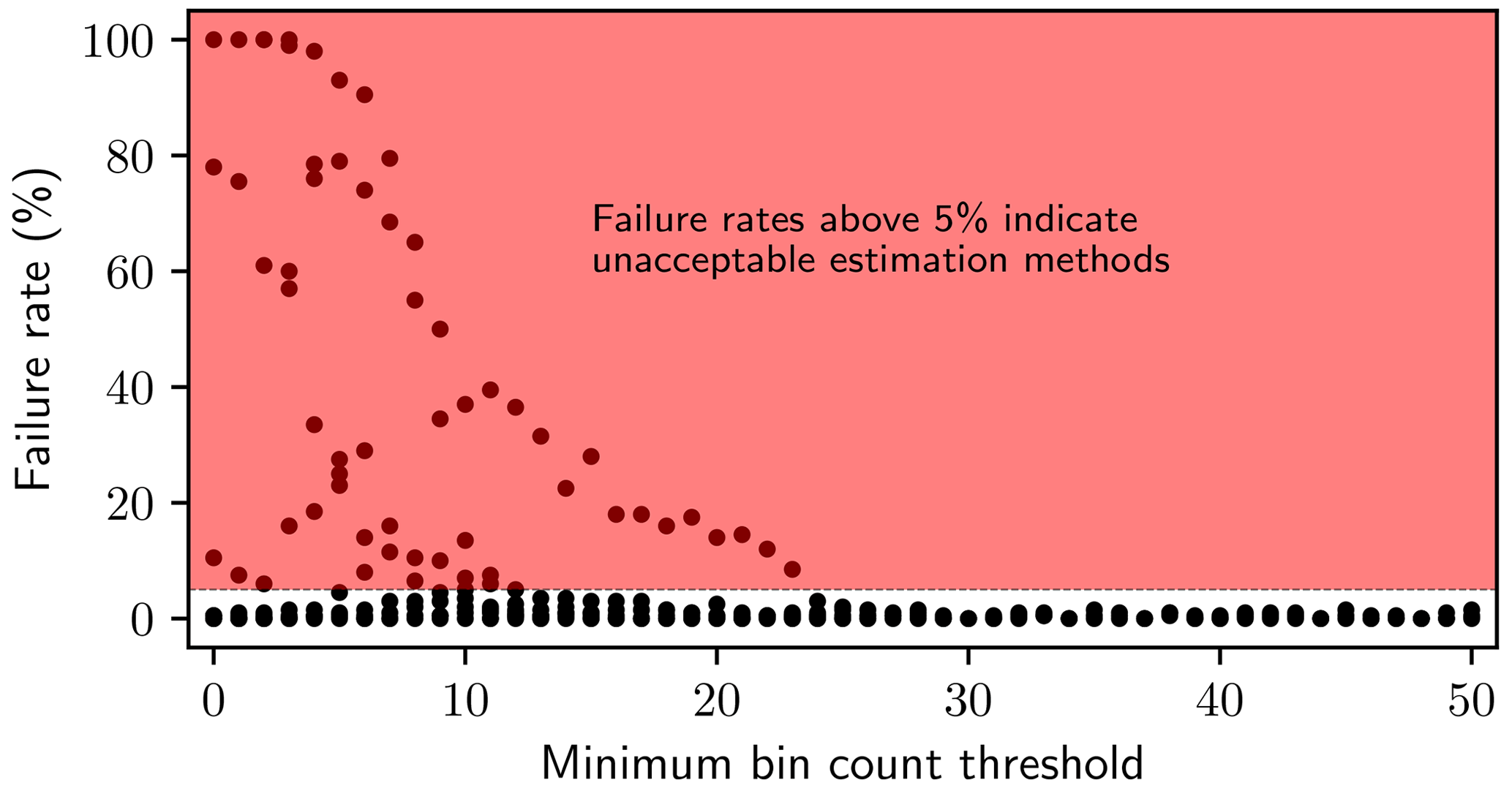
Figure 2 Failure rates for fitting α to synthetic data using a linear regression to logarithmically spaced bins, as a function of the minimum required count in each bin. Each point represents a unique combination of the number of bins, the sample size and the minimum bin count threshold. Minimum bin count thresholds greater than 24 always ensure accurate estimates of α, while smaller thresholds sometimes produce inaccurate estimates. While some points represent low failure rates for low bin count thresholds, these thresholds cannot be relied on as their accuracy depends on the sample size and number of bins.

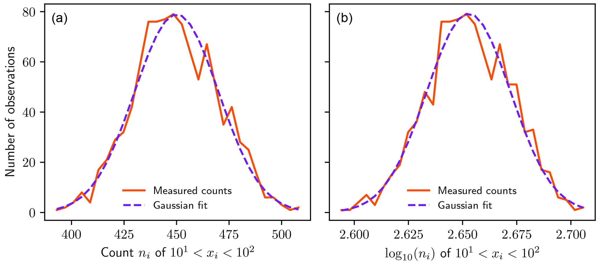
Figure 3 Statistical error in measured counts n_i (a) or log n_i (b) within a bin bounded by 10 and 100 for a collection of 1000 samples, each containing 5000 randomly generated power-law-distributed random variables x_i with exponent α=1 (Eq. 1). Each sample has a count n_i in the bin, and the plot shows a histogram of these counts n_i for all 1000 samples. The plot is thus a “histogram of histograms”. The p values for normality using a Kolmogorov–Smirnov test are 0.333 for n_i and 0.326 for log n_i, indicating that the null hypothesis of Gaussian variability cannot be excluded using a 95 % confidence threshold in either case. Table A1 shows p values for more combinations of bin location and sample size.

Applying a simple rule that least-squares linear regression only be applied to those bins with sufficiently large counts may seem obvious: estimating any statistical measure using a very small sample tends to result in error. In this particular case of statistically independent measurements, the low failure rates for high minimum bin count thresholds can be understood in terms of the central limit theorem, where the successive measurement and binning of power-law-distributed variables can be interpreted as a counting process (see Appendix A). Provided bin counts n_i exceed approximately 24, statistical error in both counts and the logarithm of the counts follows a Gaussian distribution (Fig. 3). In this case, general-purpose linear regression packages that assume Gaussian error at each point may be used to accurately estimate the exponent of a power law distribution.

In summary, whether binning is done linearly or logarithmically, there may be bias in previously calculated values of α for cloud area distributions that are power-law-distributed, but only if bins with fewer than 24 counts are included in the regression. A very simple fix is to omit such bins. Other studies that estimated α over a range of scales that exclusively included large bin counts (e.g., Benner and Curry, 1998; Cahalan and Joseph, 1989; Wood and Field, 2011; DeWitt et al., 2024) may have obtained estimates of α that were as reliable as maximum-likelihood-derived estimates. In fact, Mieslinger et al. (2019) estimated α for shallow cumulus using both a linear regression to logarithmically spaced bins and maximum likelihood estimation, finding that both fitting methods produced similar results.

Clauset et al. (2009) state that, while a histogram that is linear when logarithmically transformed is not sufficient to identify a power law distribution, linearity is certainly necessary. The challenge with cloud sizes is that some portions of the cloud size distribution appear linear in some studies but are clearly nonlinear in others. For example, Cahalan and Joseph (1989), Benner and Curry (1998) and Neggers et al. (2003) all find a scale break at ∼ 1 km², where a power law regime transitions to an exponential or a different power law with a much larger value of α. Either case indicates a clear nonlinear portion of the doubly logarithmic histogram at or beyond the scale break. This is in disagreement with other studies that find linear power law scaling up to ∼ 10 km² or ∼ 100 km² (van Laar et al., 2019; Savre and Craig, 2023) and especially with the findings of power law scaling extending beyond 10⁵ km² (Wood and Field, 2011; Christensen and Driver, 2021; DeWitt et al., 2024). Differences in the choice of fitting method used, whether maximum likelihood estimation or regressions to linearly or logarithmically spaced bins, cannot explain these differences in measured a_max. While differences in meteorological conditions may contribute, meteorological influences may still be obscured by methodological problems. We next explore how the improper treatment of clouds that are truncated by the edge of the measurement domain could influence measured size distributions.

3 How a finite domain changes measured size distributions

Truncated clouds, which span the domain edge (Fig. 1), present a conundrum. If one wants to accurately measure the size distribution within a finite domain, should one remove them from consideration, risking undercounting clouds in some size classes, or should the clouds be included, risking inaccurate area measurements? To investigate the magnitude of this truncation effect, we explore measured size distributions for various domain sizes.

3.1 Atmospheric cloud measurements, the percolation model and domain subsampling

For measurements of atmospheric clouds, we use data from the Advanced Baseline Imager (ABI) aboard the GOES-West (GOES-17) satellite. GOES-West is a geostationary satellite centered at 137° W with a nadir-imaging resolution of approximately 2 km. A preprocessed cloud mask product that attempts to identify every pixel as “cloudy” or “clear” is used, and so each “image” is a binary array of pixels specified as 1 for cloudy or 0 for clear. A total of 10 processed images are used, each taken at local noon (21:00 UTC) between 1 and 10 June 2021.

We use the 2000×2000 pixels located in the center of the image and approximate all pixel dimensions as 2 km × 2 km, which underestimates the true pixel length dimensions by at most 12 %. The chosen domain is in the central Pacific between longitudes of 117 and 157° W and latitudes of 19° S and 19° N. There are no missing data for the domain and time period considered. Because clouds are fractal, clouds made up of a small number of pixels appear unrealistic because their shapes are overly influenced by the shape of non-fractal square pixels (Christensen and Driver, 2021). Thus, fits for the power law exponent are restricted to cloud areas larger than 10 times the area of 1 pixel (DeWitt et al., 2024).

We also consider size distributions for more idealized objects. The uniform square lattice, adopted from percolation theory, is a two-dimensional square lattice where every site (or cell) is occupied with uniform probability ℙ. “Clusters” are defined as regions of adjacent occupied sites (Stauffer and Aharony, 1992), and their area a is defined as the number of occupied sites in a single cluster. The mean cluster area 〈a〉 tends to increase with increasing ℙ because a high site occupation probability increases the likelihood of site connection (Stauffer and Aharony, 1992).

A central result of percolation theory is that, as ℙ approaches a critical point ℙ_c≈0.592746…, 〈a〉 tends to infinity and the distribution of cluster areas follows a power law $n\left(a\right)\propto a^{-\mathit{\tau }}$, where $\mathit{\tau }=\mathrm{187}/\mathrm{91}$. The power law is only exact in the limit of large clusters and an infinite lattice but serves as a close approximation to the size distribution of clusters that are larger than about 10 to 20 sites (Stauffer and Aharony, 1992). In finite lattices, the size of the largest cluster is limited by the size of the lattice, and so the power law regime cannot extend to arbitrarily large scales as it does for an infinite lattice. This “cutoff” is often modeled by an exponential function $n\left(a\right)\propto a^{-\mathit{\tau }}{e}^{-a/a_{\text{c}}}$, where a_c is the characteristic area of the largest clusters, a function of lattice size (Stauffer and Aharony, 1992).

The percolation model is useful here for studying distributions of object size distributions in finite domains because the distribution of cluster sizes is known exactly. In particular, any deviation from power law scaling at the large end of the cluster size distribution is known to exist because the lattice has a finite size. Models similar to the uniform square lattice used here have also been leveraged previously to explain the fractal dimension of precipitating regions (Peters et al., 2009) and of the power law scaling in cloud sizes itself (Savre and Craig, 2023).

We simulate three 10 000 × 10 000 percolation lattices at the percolation threshold ℙ=0.592746. For both the GOES-derived cloud masks and the percolation lattices, clouds or clusters are defined according to the convention that adjacent pixels are considered connected and diagonals are not. This is standard practice in both percolation theory (Stauffer and Aharony, 1992) and past cloud studies (e.g., Kuo et al., 1993; Wood and Field, 2011). Individual object areas are calculated by summing connected pixel areas, and an object is flagged as “truncated” if it is connected to the lattice boundary (Fig. 1).

To test how the domain or lattice size affects the measured area distributions, the binary arrays representing cloud fields or percolation lattices are subdivided as follows: if the shape of the original array is L×L grid points, with L=10 000 for the percolation lattices and L=2000 for the GOES-West images, subarrays are created by choosing a value q and dividing the original array into subarrays of size $L/q\times L/q$. We use values of $q\in \mathit{\{}\mathrm{5},\mathrm{50},\mathrm{200},\mathrm{500}\mathit{\}}$ for the percolation lattices and values of $q\in \mathit{\{}\mathrm{10},\mathrm{40},\mathrm{100}\mathit{\}}$ for GOES images. Thus the percolation subarrays have side lengths of 2000, 200, 50 or 20 grid cells, which match the dimensions of the original GOES array and its subarrays.

3.2 Measured size distributions as a function of domain truncation effects

For each subdomain considered in the cloud imagery, if truncated clouds are removed from the size distributions, bin counts are increasingly undercounted at larger object areas as shown in Fig. 4. A spurious scale break is introduced at these sizes that resembles an “exponential tail”, a functional form suggested by Savre and Craig (2023) as being a real characteristic of clouds under certain circumstances. The form of the scale break also resembles many prior findings for both simulated and observed clouds (e.g., Cahalan and Joseph, 1989; Benner and Curry, 1998; Neggers et al., 2003; Heus and Seifert, 2013; Senf et al., 2018; van Laar et al., 2019; Christensen and Driver, 2021). The locations of the spurious scale breaks, like those proposed in the literature, span several orders of magnitude but only depend on the domain size. A scale break is introduced because larger clouds are more likely to be truncated and therefore removed from the analysis (Fig. 5). This effect occurs for all the domain sizes. The clouds need not be particularly large to be affected, as the scale break appears at surprisingly small cloud areas occupying between 1 % and 0.1 % of the subdomain area.

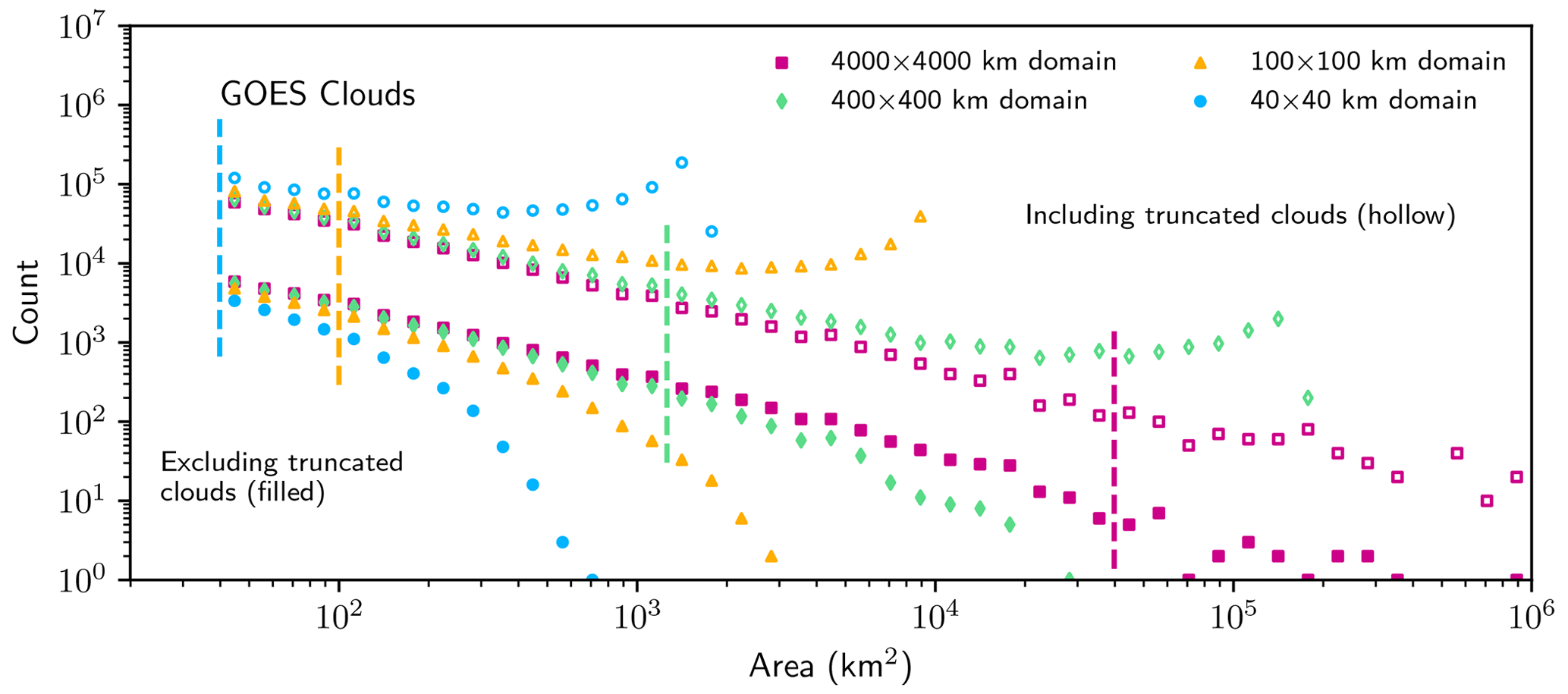
Figure 4 Histograms of cloud areas for several sizes of subdomains from GOES-West. Filled shapes indicate histograms which do not include truncated clouds, while hollow shapes include truncated clouds. Hollow shapes are offset vertically by a factor of 10 for clarity. The vertical dashed lines mark the smallest bin in which 50 % of the objects are truncated by the domain edge for each domain size.

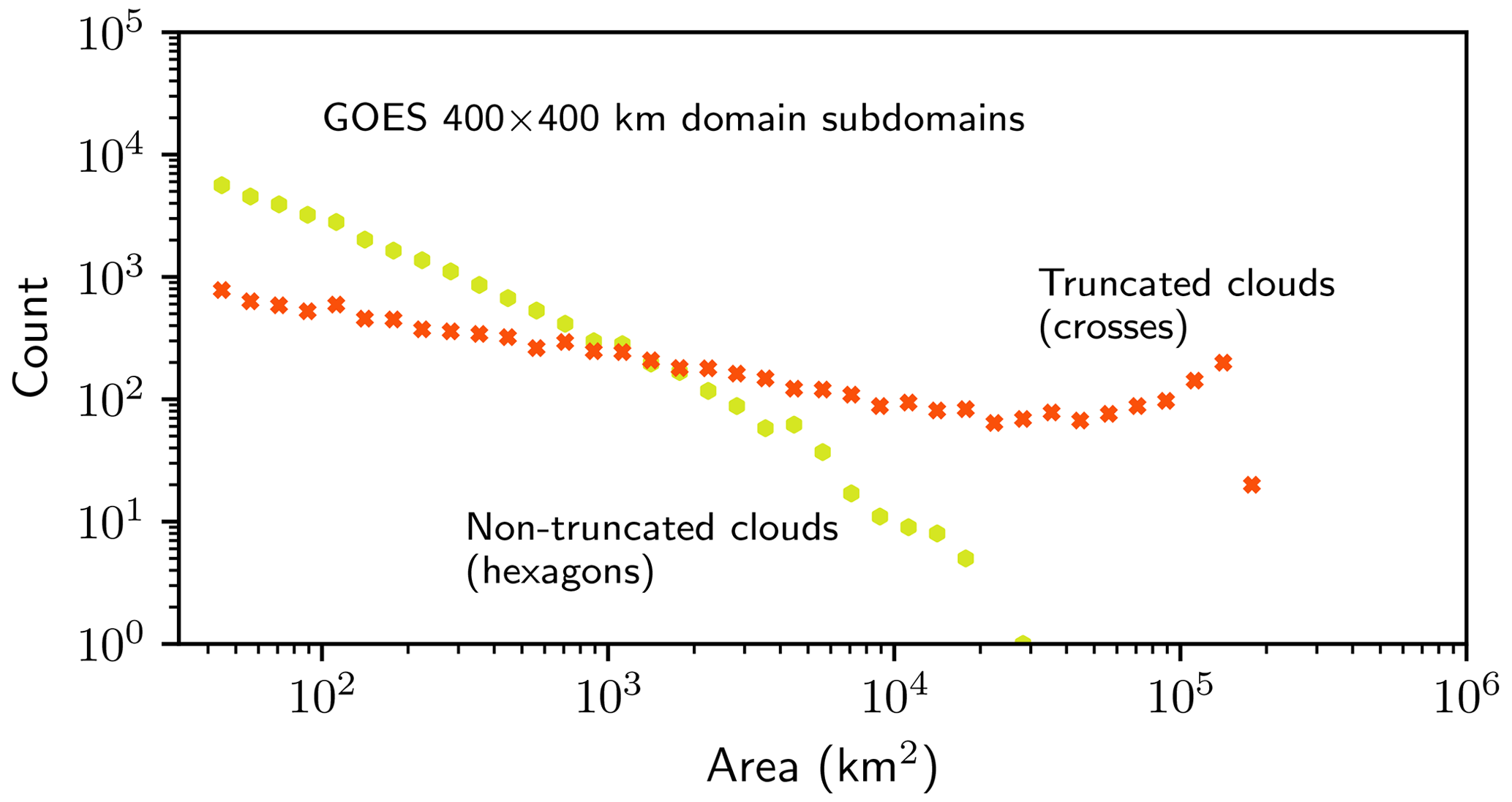
Figure 5 Histogram of cloud areas measured in the 400×400 km subdomains, as in Fig. 4, but separated into those that are truncated by the edge of the domain (crosses) and those that are not (hexagons). At small areas, the number of truncated clouds is negligible compared to the number of non-truncated clouds, but at larger areas the pattern reverses and the number of non-truncated clouds becomes negligible relative to the number of truncated clouds.

Alternatively, if truncated clouds are included in the histogram, they are placed in a smaller-size bin than that in which they belong. This leads to an overcount for all the bins, particularly for large clouds and a spurious local maximum in cloud frequency for clouds with areas close to the domain area.

Figure 6 As for Fig. 4 but for cluster areas in the percolation lattices.

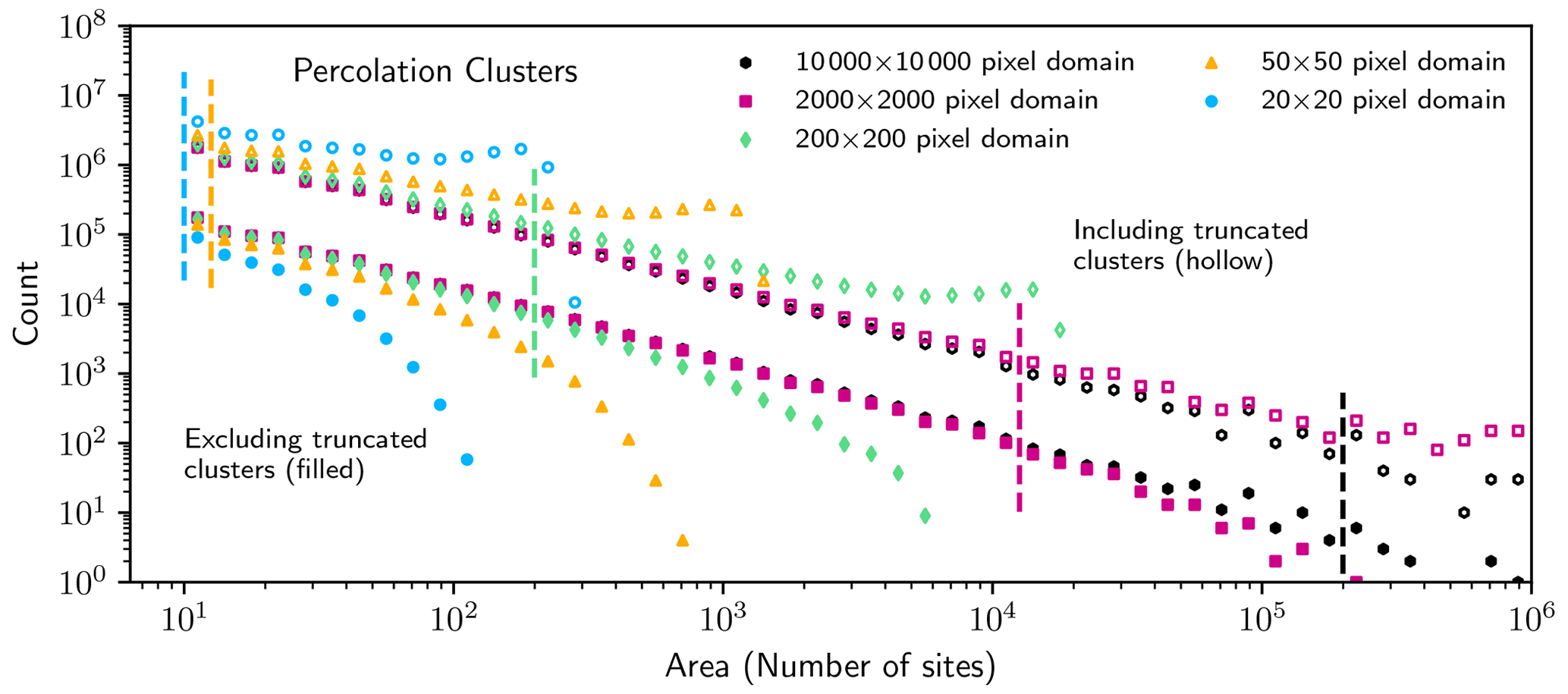
The effect of miscounting large clouds in a finite domain is also mirrored in the percolation lattices, where either a cutoff regime (an undercounting) or a local maximum (an overcounting) is introduced into the size distribution, respectively (Fig. 6). Because percolation clusters are known to follow a power law size distribution, the undercounting or overcounting can only be caused by the finite size of the lattice. This illustrates how truncation effects are not limited to atmospheric clouds but could affect measured size distributions of any phenomenon that is measured within a finite domain.

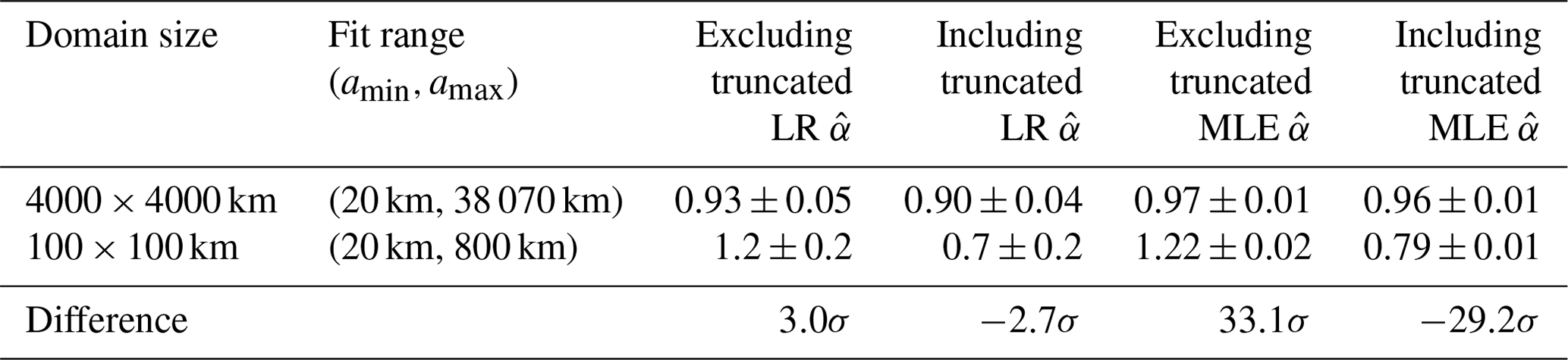
Table 1 Fits from the hypothetical scenario where cloud areas are measured within the 100 × 100 km GOES subdomains and fits are obtained over a subjectively defined linear region (Fig. 7). Fits are obtained using both linear regression (LR) as described in the text and maximum likelihood estimation (MLE) as described by Savre and Craig (2023). Errors for MLE fits are calculated using a standard bootstrapping procedure and correspond to the 95 % confidence interval. For comparison, fits to clouds measured in the full domain are included as “truth”. “Difference” is the difference in $\widehat{\mathit{\alpha }}$ between the two domain sizes. The difference is expressed in units of standard errors as calculated from the subdomains.

The simple remedy of calculating α by fitting a power law over a relatively linear region of the distribution that is subjectively defined, as is often done, can lead to an overestimate of α if truncated clouds are removed and an underestimate if they are included. As an example, Fig. 7 depicts a hypothetical scenario where the cloud area distribution is measured using images that all cover a domain 100×100 km in size. For this purpose, we use all the 100×100 km subdomains from GOES. Values of α are calculated over a subjectively defined linear range of scales for both cases of including and excluding truncated clouds in the distribution. Regardless of whether least-squares linear regression or maximum likelihood estimation is used, including truncated clouds in the fit for α leads to underestimates of 36 % and 19 %, respectively, while excluding them leads to overestimates of 24 % and 20 %, respectively, relative to values calculated for the full 4000×4000 km domain (Table 1). These errors would be greater if larger area values were included in the fit or if the domain were smaller. Nonetheless, it is clear from Fig. 7 that both approaches remain well-approximated by a power law distribution, and so the truncation effect could easily be missed if only one approach was presented. This would lead to reported power law behavior with a value of α that is a significant departure from the true value that would have been measured if the domain had been larger.

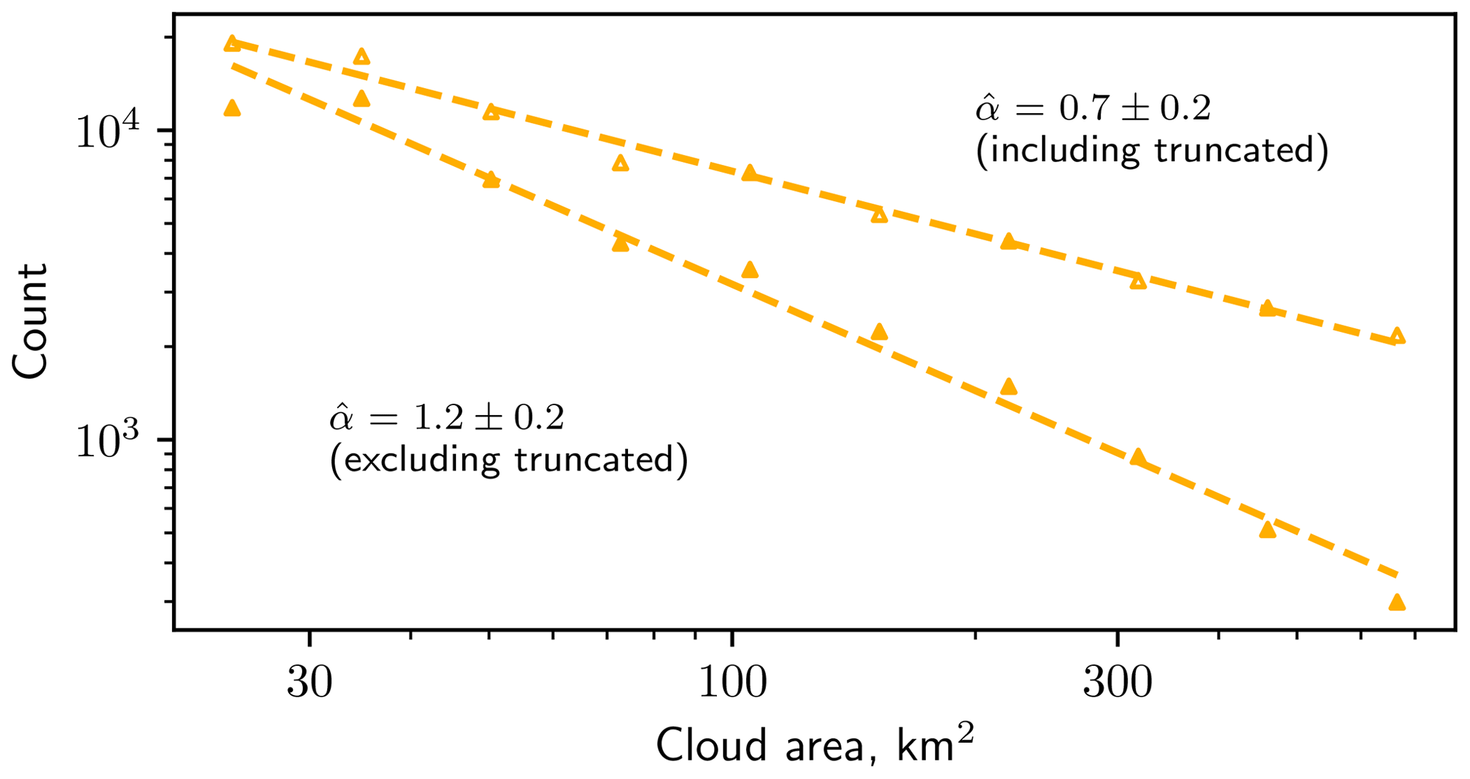
Figure 7 Example of how a measurement $\widehat{\mathit{\alpha }}$ of the power law exponent could be biased by whether or not truncated clouds are included in the analysis. The histograms shown are created using all 100×100 km subdomains from GOES. The same histograms are shown in Fig. 4 but spanning a wider range of scales. This particular range of scales is heavily influenced by the choice of including truncated clouds. Fits for α are shown in Table 1.

We recommend, as a simple solution for the errors introduced by domain truncation effects, only analyzing bins containing a small number of truncated clouds n_truncated relative to the total in each bin n_total. Because larger clouds are more likely to be truncated by the domain edge (Fig. 5), this procedure effectively removes the large end of the size distribution from the fit. Conveniently, in practice this procedure sometimes also enforces the minimum bin count threshold of 24 that is necessary for reliable linear-regression-derived fits for the power law exponent.

Table 2 Estimated values of α (denoted as $\widehat{\mathit{\alpha }}$) to cloud areas measured within the full domain and subdomains over the region where $n_{\text{truncated}}/n_{\text{total}}<\mathrm{0.5}$ as a function of the choice of including or excluding truncated clouds in the fit. Only those subdomains in which the fitting region spans at least 1 order of magnitude are included. Fits are obtained using both linear regression (LR) as described in Sect. 2 and maximum likelihood estimation (MLE) as described by Savre and Craig (2023). Errors for MLE fits are calculated using a standard bootstrapping procedure and correspond to a 95 % confidence interval.

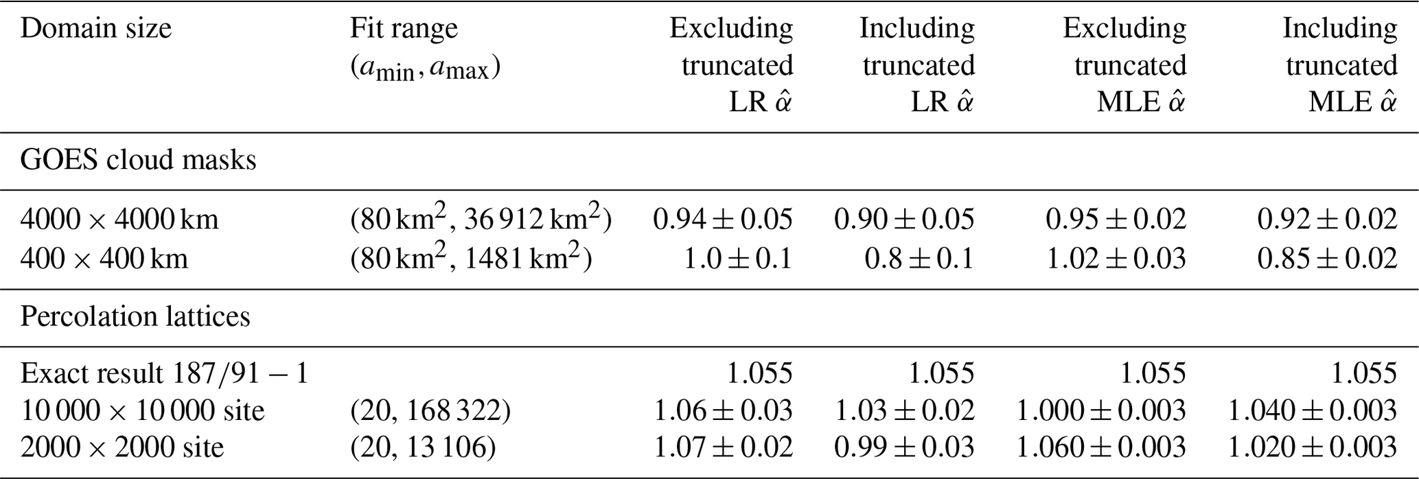
In Table 2, estimates of α are listed for the region where $n_{\text{truncated}}/n_{\text{total}}<\mathrm{0.5}$ for a series of subdomains created from the GOES cloud masks and the percolation lattices. Although imperfect, when a 50 % threshold is used, fitted values for α are much less sensitive to the choice of fitting method or whether truncated clouds are included or removed. The 50 % threshold represents a compromise between allowing for a significant range of scales to be analyzed and removing those bins most affected by truncation effects. A more stringent threshold of 10 % (not shown) was found to produce similar results but to omit a larger portion of the distribution from the fit.

Regardless of the domain size, truncation effects occur. For robust power law fits, the resolution ξ must be sufficiently small so that the distribution spans the recommended 2 orders of magnitude (Stumpf and Porter, 2012) even after the 50 % threshold is applied. For the square domains considered here, using a lower limit for the fit of $a_{min}=\mathrm{10}{\mathit{\xi }}^{\mathrm{2}}$, we find that the domain length L must be on the order of $L/\mathit{\xi }\sim \mathrm{300}$ to satisfy this requirement.

In principle, because the 50 % threshold removes larger objects in the distribution that may be of scientific interest, an algorithm could be devised to correct cloud truncation effects. One such algorithm was used by Wood and Field (2011). However, it was assumed that clouds are square-shaped. In general, any correction algorithm requires some similarly questionable assumption, and so considerable caution should be exercised when devising such an algorithm. This issue is discussed further in Appendix B.

3.3 Finite-domain effects in periodic domains

One commonly employed method for reducing artifacts caused by domain boundaries in cloud simulations is to utilize doubly periodic simulations that allow fluxes out of one side of the numerical grid to re-enter on the opposite side (e.g., Neggers et al., 2003; Yamaguchi and Feingold, 2013; Heus and Seifert, 2013; Garrett et al., 2018). Unfortunately, even without a domain edge, simulations with periodic domains still suffer from a finite domain area that modifies the cloud size distribution. For example, consider the limiting case of a model composed of a single horizontal grid cell. Even with a periodic domain that maintains flux conservation laws, the cloud size distribution would nonetheless be unphysically constrained to one possible cloud size, leaving α undetermined.

The impact of employing periodic domains may easily be examined within percolation lattices. Because each site has an occupation probability that is independent of the surrounding sites, the model can be made periodic simply by changing the site connectivity to be periodic at the lattice boundaries. Specifically, if a lattice of size L×L sites has coordinates (i,j) and if both sites (1,b) and (L,b) are occupied, they are defined as part of the same cluster for any index b. Similarly, sites (c,1) and (c,L) are also part of the same cluster when both are occupied for any c.

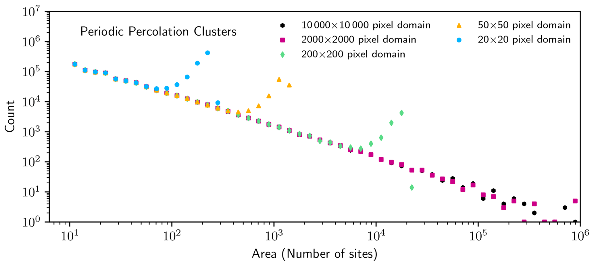
Figure 8 Histogram of cluster areas in doubly periodic percolation lattices for several domain sizes.

In this case, as Fig. 8 shows, size distributions in periodic percolation lattices remain strongly influenced by the finite lattice size, appearing qualitatively similar to those measured in non-periodic lattices with truncated clusters included in the size distribution (Fig. 6). That is, distributions have a local maximum for cluster areas that are similar to the area of the domain. Such a local maximum is an example of a non-power law size distribution that is not representative of the power law cluster size distribution that is known to characterize a larger lattice. The implication is that periodic boundary conditions cannot be adopted as a fix for finite-domain effects on a measured size distribution.

3.4 Finite-domain effects for exponential distributions

Even if the distribution of object sizes does not follow a power law, domain truncation effects may still bias measured size distributions. As an example, consider the distribution of raindrop sizes as measured by the new Differential Emissivity Imaging Distrometer (DEID). The DEID measures raindrop mass by measuring the time it takes for raindrops to evaporate after landing on a hotplate (Rees et al., 2021). Water drop areas and lifetimes can be estimated from images of the hotplate, from which precipitation rates and size distributions can be estimated based on first-principles heat transfer physics. Because the procedure requires calculation of size distributions of droplets within a finite two-dimensional image, drop size distribution estimates may be affected by droplets truncated by the edge of the image in a similar manner to images of cloud fields taken by a satellite.

The main difference between precipitation and cloud size distributions is that precipitation size distributions tend to follow an exponential rather than a power law (Marshall, 1948; Singh et al., 2023). Nonetheless, removal of truncated droplets from the analysis would still influence the measured distributions. This can be illustrated by examining a manufactured exponential distribution. For this purpose, we create a percolation lattice with a site occupation probability just smaller than the critical probability ℙ_c. In this case, analytical results suggest that cluster sizes follow a power law with an exponential tail (Stauffer and Aharony, 1992). The characteristic cluster size of the exponential tail increases without bound as the site occupation probability approaches ℙ_c.

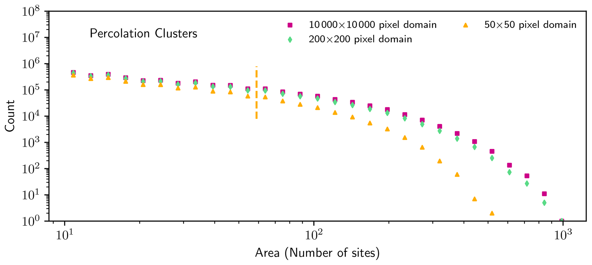
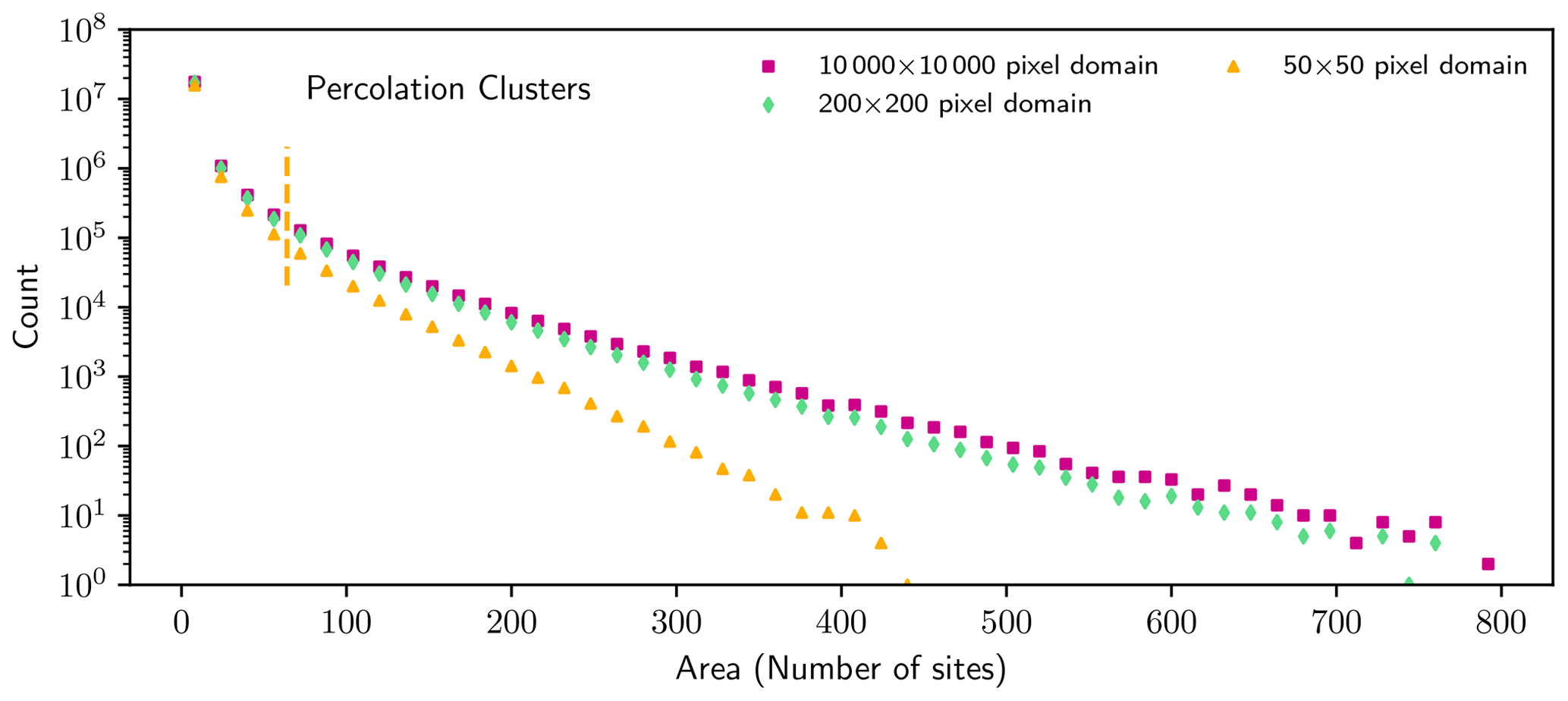
Figure 9 Histogram of percolation cluster areas generated in lattices with a site occupation probability equal to 0.5. Plotted counts do not include truncated clusters. For the 50×50 lattices, as in Fig. 6, truncated clusters outnumber non-truncated clusters in bins to the right of the dashed yellow line. For the larger domains, there are no bins that contain a majority of truncated clusters.

Figure 9 shows histograms of cluster sizes calculated from percolation lattices with a site occupation probability equal to ℙ=0.5 for several sizes of lattice subdomains. As shown in Appendix C, in this case the cluster size distribution is exponential for clusters larger than ∼ 200 sites. The fraction of truncated clusters, relative to the total for each bin, never exceeds 50 % in the 10 000×10 000 and 200×200 lattices, indicating that truncation effects are insignificant. However, a histogram taken from the 50×50 lattices is strongly influenced by the removal of truncated clusters, thus undersampling large clusters relative to sampling done within a larger domain.

As with power laws, sufficiently large bins in an exponential distribution are dominated by truncated clusters. Applying the same 50 % truncated cluster criterion provides a straightforward method to identify which bins are most influenced by the choices of including or removing truncated clusters. A more accurate size distribution can still be obtained provided that these bins are omitted from the fit.

4 Conclusions

There is significant disagreement in the literature on what the appropriate choice of distribution should be to describe cloud horizontal areas. Most studies find that cloud areas follow a power law $n\left(a\right)\propto a^{-(\mathit{\alpha }+\mathrm{1})}$, although there is considerable disagreement on the range of scales over which the power law applies and the value of α. A recent study proposed that, while differences in local climatological characteristics contribute to variability, some of the disagreement is due to the use of inferior linear-regression-based fitting methods, arguing that maximum-likelihood-based methods are superior (Savre and Craig, 2023).

The present study shows that the choice of fitting method cannot explain the disagreement among observations, particularly for the range of scales over which a power law applies. We find that a linear regression to logarithmically spaced bins is an equally accurate fitting method for power-law-distributed data provided the simple requirement is adopted that bins with fewer than ∼ 24 counts are omitted from the regression. Linear regression also has the advantage of being computationally trivial and more conceptually straightforward than maximum-likelihood-based alternatives.

We suggest that different accounts of cloud power law behavior in the literature are best explained by treatments of clouds whose geometries are “truncated” by the edge of the measurement domain. Removal of truncated clouds from the distribution introduces an artificial “cutoff scale” beyond which clouds can be significantly undersampled, with a resulting distribution consistent with many previous findings (e.g., Cahalan and Joseph, 1989; Benner and Curry, 1998; Neggers et al., 2003; Heus and Seifert, 2013; Senf et al., 2018; van Laar et al., 2019; Christensen and Driver, 2021). If included, a local maximum in the distribution appears at areas comparable to the domain scale that does not reflect the true distribution. Even when a periodic domain is used, measured size distributions do not reproduce the size distributions that would be obtained in larger domains. In any case, a power law may still easily be measured, but the value of the power law exponent could be underestimated or overestimated by 20 % to 30 % or more.

While size distributions measured within any domain size are affected by truncation effects, they are most important only for the largest clouds. The affected scale is easily identified by counting for each bin the fraction of clouds that are truncated relative to the total in that bin. We recommend that power law fits be applied only to bins in which the fraction of these clouds is less than 50 %.

Truncation effects are not limited to power law size distributions, as exponentially distributed objects can be similarly affected. Fortunately, the 50 % truncated object criterion is applicable regardless of the underlying form of the distribution.

The issues and remedies discussed here are not specific to atmospheric clouds and can be applied to size distributions characterizing any other phenomena measured within a finite geometric domain, e.g., with ecological predator–prey models (Pascual et al., 2002), CO₂ pockets in sedimentary rocks (Iglauer et al., 2010), snowflakes (Rees et al., 2021), cloud droplets (Beals et al., 2015), aerosols (Magín Lapuerta and Gómez, 2003) and soil particles (Mora et al., 1998).

Appendix A: Statistical variability in histogram bin counts

The result that linear-regression-based fitting methods can accurately estimate the power law exponent α, provided that bins with counts less than ∼ 24 are omitted from the regression, might appear to contradict the results of Clauset et al. (2009). They argued in their Appendix A that linear-regression-based estimation methods for α are biased. In this section, we explain their argument why linear regression can in fact be accurate, and point out a subtle error made in the widely cited work by Clauset et al. (2009).

The central issue is the statistical error of bin counts in a histogram. As a conceptual model, consider a large number of experiments that all measure some variable many times and bin the results into a histogram. The count in each bin can be expected to be roughly similar from experiment to experiment but not exactly the same. The “statistical error” is the standard deviation of the bin counts, which could be estimated, e.g., by sampling a large collection of experiments.

This conceptual model can be made more precise by considering the experiments to be a random counting process consisting of N independent and identically distributed draws of a random variable X from an arbitrary distribution. Consider some bin i of fixed size and location in the parameter space of X. The “bin count function” n_i may be introduced by first considering an indicator function 𝕀 which is equal to 1 if X lies within i and 0 otherwise. The bin count n_i is simply the sum of 𝕀 over all draws.

The advantage of introducing 𝕀 is that the central limit theorem applies to 𝕀 even if it does not to X. Specifically, the theorem requires independent, identically distributed random variables, a finite variance and a finite mean. Because the mean value 〈𝕀〉 and the variance σ² of 𝕀 are both bounded by 0 and 1, these assumptions are satisfied, and therefore the central limit theorem states that the bin count n_i tends to a Gaussian distribution as N→∞.

Standard linear regression packages assume that each data point has Gaussian error. In their Appendix A, Clauset et al. (2009) argued that linear-regression-based estimation methods are invalid if the regression is performed to log n_i, which is supposedly not Gaussian if n_i is Gaussian.

This is incorrect because the central limit theorem also states that the variance of n_i tends to ${\mathit{\sigma }}^{\mathrm{2}}\sqrt{n_i}$ (where σ²≤1 because $\mathrm{0}\le \mathbb{I}\le \mathrm{1}$), and so the standard deviation of n_i is $\mathit{\sigma }{n}_i^{\mathrm{1}/\mathrm{4}}\ll n_i$ for large n_i. This means that almost all errors ε are much smaller than n_i, and so we may linearize log (n_i+ε) using a Taylor expansion about n_i so that

$$\begin{array}{}\text{(A1)}& \log \left(n_i+\mathit{\epsilon }\right)\approx \log n_i+{\displaystyle \frac{\mathit{\epsilon }}{n_i}}+\mathcal{O}\left({\displaystyle \frac{{\mathit{\epsilon }}^{\mathrm{2}}}{n_i^{\mathrm{2}}}}\right).\end{array}$$

​​​​​​​Thus, in the neighborhood of n_i, the logarithmic transformation is linear if terms of order $\mathrm{1}/n_i^{\mathrm{2}}$ are neglected. Because the transformation is linear, log n_i is also Gaussian-distributed, in which case linear regression packages estimate both errors and the power law exponent itself accurately for large n_i. The requirement of a large n_i is not a significant one because it is in fact required even for n_i to be Gaussian, because n_i is a discrete quantity.

Table A1 Kolmogorov–Smirnov p values, as in Fig. 3, for more combinations of bin location, sample size and α. Combinations are excluded if the mean n_i is less than 3. With two exceptions, every case where the null hypothesis of normality in log n_i would be rejected using a 95 % confidence interval (bold) has a mean count that is less than 24. In the two exceptions, the null hypothesis would still be rejected if the confidence interval were raised to 99 %. This is roughly consistent with the expectation that 1 in 20 experiments would result in a false conclusion using a 95 % confidence interval.

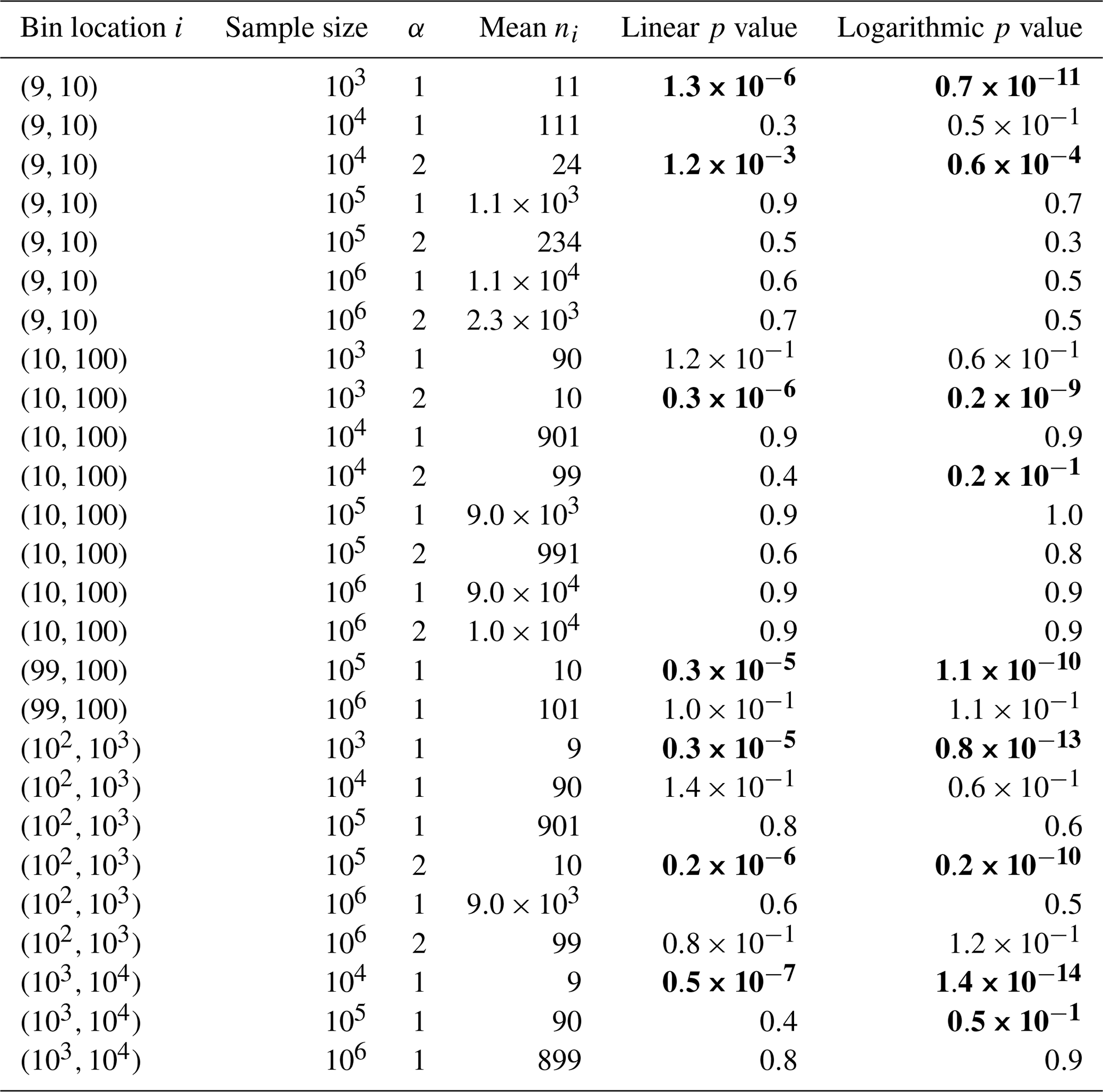
Figure 3 shows an empirical test of the above reasoning, where 1000 samples, each containing 5000 randomly generated numbers, were drawn from a power law distribution with α=1. The bin $\mathrm{10}<x_i<\mathrm{100}$ showed Gaussian variability in the bin count n as well as the log of the bin count log n, as illustrated by nearly identical Kolmogorov–Smirnov p values (0.333 vs. 0.326, respectively). Table A1 shows Kolmogorov–Smirnov p values for more combinations of bin location and sample size.

We suggest that this result explains why the linear regression technique used in Sect. 2 is accurate. Previous results, including those of Clauset et al. (2009), may have produced biased power law exponents simply because they included bins with small n_i in the linear regression. If such bins are excluded from the linear regression, statistical errors of log n_i are approximately Gaussian-distributed and estimations of power law exponents can be accurately estimated within normal measurement uncertainties.

Are cloud sizes statistically independent?

The above argument applies to measurements that are statistically independent because statistical independence implies that the bin count n_i has Gaussian error. The maximum likelihood estimation method presented by Clauset et al. (2009) also requires statistically independent errors. Unfortunately, statistical independence is often not satisfied in physical systems such as naturally occurring networks (Serafino et al., 2021) and clouds (Garrett et al., 2018). Because cloud formation is constrained by the total available moisture, energy and space, individual cloud areas are not physically independent, and this appears in the statistics. For example, a large but rare cloud that covers over half of a given measurement domain makes it impossible to observe another similarly sized cloud because a second large cloud could not fit inside the domain. Thus, the first observation (i.e., the large cloud) alters the probability of the next observation, which violates statistical independence. Similarly, a finite amount of total available energy or moisture makes future cloud formation contingent on what has occurred in the past. Thus, statistical errors of n_i may not be Gaussian, in which case maximum-likelihood-estimation-based methods would be inappropriate.

A priori, one might expect statistical errors for cloud sizes to be lognormal instead (implying that log n_i is Gaussian), because scale-by-scale conservation of a relevant variable ϕ implies that ϕn_i is constant (because the total amount Φ within a bin is ϕn_i). As an example, Garrett et al. (2018) identified cloud perimeters p as controlling cloud formation in thin quasi-horizontal layers. By assuming pn_i=const., they derived a power law distribution for cloud perimeters. Similarly, in their Sect. 3.3, Lovejoy and Schertzer (2013) argue for a “multiplicative central limit theorem” for energy flux, which implies that the logarithm of the energy flux is Gaussian-distributed.

Regardless, lognormality in statistical errors of n_i is a convenient assumption when using linear-regression-based methods to estimate a power law exponent, because in this case log n_i is Gaussian, as software packages assume. However, it is conceivable that statistical errors of cloud area measurements might follow a different distribution, in which case neither maximum likelihood estimation nor linear regression would be strictly appropriate. Another problem with either method could be heteroscedasticity: that is, the variance of n_i could depend on cloud size. This could be due to either physical differences in the spatial scale or the effect of the finite domain size. Further work is needed to determine both the shape of the distribution of n_i as well as its dependence on the spatial scale.

Appendix B: Correction algorithms for domain truncation effects

The method we propose to address domain truncation effects, i.e., to omit bins in which the truncated clouds are greater than 50 % of the total, effectively removes a large portion of the size distribution. If the large portion is of interest, an algorithm could be derived in principle for the effects of the removal of clouds that are truncated by the domain edge.

Consider the case of cloud area distributions. If cloud locations are statistically independent of the domain edge location, the probability of a cloud being truncated by the domain edge P_truncated(a), a function of cloud area a, can be calculated from the mean cloud “lengths”, defined as the longest distance from one end of the cloud to the other in the orthogonal x and y dimensions of an image. If cloud lengths can be related to cloud areas – which is a nontrivial problem due to fractal cloud geometries – a correction for the removal of clouds touching the edge is straightforward to implement since $n(a{)}_{\text{obs.}}=(\mathrm{1}-P_{\text{truncated}}\left(a\right)\left)n\right(a)$, where n(a) is the true cloud area distribution. Wood and Field (2011) used a similar formulation, assuming clouds were square-shaped in order to relate cloud areas to cloud lengths.

In general, obtaining an appropriate correction algorithm can be a surprisingly difficult problem. For clouds specifically, there are several issues. First, cloud lengths would likely not be proportional to $\sqrt{a}$ since clouds are fractal and the length dimensions of fractal objects do not necessarily scale with $\sqrt{a}$ (Mandelbrot, 1982). Second, on a rotating planet, cloud lengths in the zonal direction may be related to area through a different function than cloud lengths in the meridional direction, since there are different temperature, moisture and Coriolis force gradients zonally vs. meridionally, and these gradients may be functions of the horizontal scale. Third, cloud locations are not statistically independent of the domain edge location for large domains due to variability in regional climatological cloud fractions owing to, e.g., the placement of the continents or the sphericity of Earth. Finally, cloud shapes are quite variable, and so any relationship between cloud length and cloud area can only be expressed statistically.

This last point is particularly problematic, since it makes simply measuring the relationship between cloud area and cloud length difficult and affected, again, by the choice of the domain size. Consider a hypothetical case where most large clouds are much longer zonally than they are meridionally but whose dimensions are measured in a square domain. The only clouds whose zonal lengths can be accurately estimated are those not truncated by the western or eastern sides of the domain. Such clouds will be predominately not wider zonally than meridionally because the zonally wider clouds will be truncated and subsequently removed from the analysis. The measured sample will be heavily biased away from zonally wide clouds, skewing the measured relationship between cloud length and area.

For a more in-depth exploration of the subtleties involved in correcting object size distributions, see Chap. 4 of the MS thesis by DeWitt (2023).

Appendix C: Validation of exponential distributions of percolation clusters

To create an exponential distribution of cluster sizes, in Sect. 3.4 we create percolation lattices with a site occupation probability equal to 0.5. Theoretically, this should result in a cluster size distribution that follows a power law with an exponential cutoff. This is supported by Fig. C1, which shows that the calculated histograms are indeed linear on a log-linear plot for a≳200 sites, which is a requirement for an exponential distribution.

Interestingly, the 40×40 subdomains, which are strongly influenced by the removal of truncated clusters, also result in an apparently exponential distribution but with a steeper slope. Such exponential behavior cannot continue to arbitrarily large cluster areas, however, because a pure exponential tail would predict a nonzero probability of observing a cluster that is larger than the lattice itself, which is impossible if truncated clusters are removed.

Figure C1 As in Fig. 9 but with the x axis on a linear scale.

Appendix D: Tables of linear regression failure rates

Tables D1 and D2 display failure rates for the selected linear-regression-based estimators for α that are plotted in Fig. 2.

Table D1 Rate of reliable estimates of the power law exponent $\widehat{\mathit{\alpha }}$ for different linear-regression-based estimation methods (“estimators”) for 200 samples. Table D2 shows additional estimators for minimum bin counts of 30 and 50. Dashes indicate estimators where at least one sample did not contain bins spanning the required 1 order of magnitude after the minimum bin count threshold was applied and thus the power law exponent could not be estimated. Errors ε are estimated as 2 standard errors on the regression and correspond to a 95 % confidence interval. Biased estimators, defined as estimators whose failure rate is more than 5 %, are marked in bold.

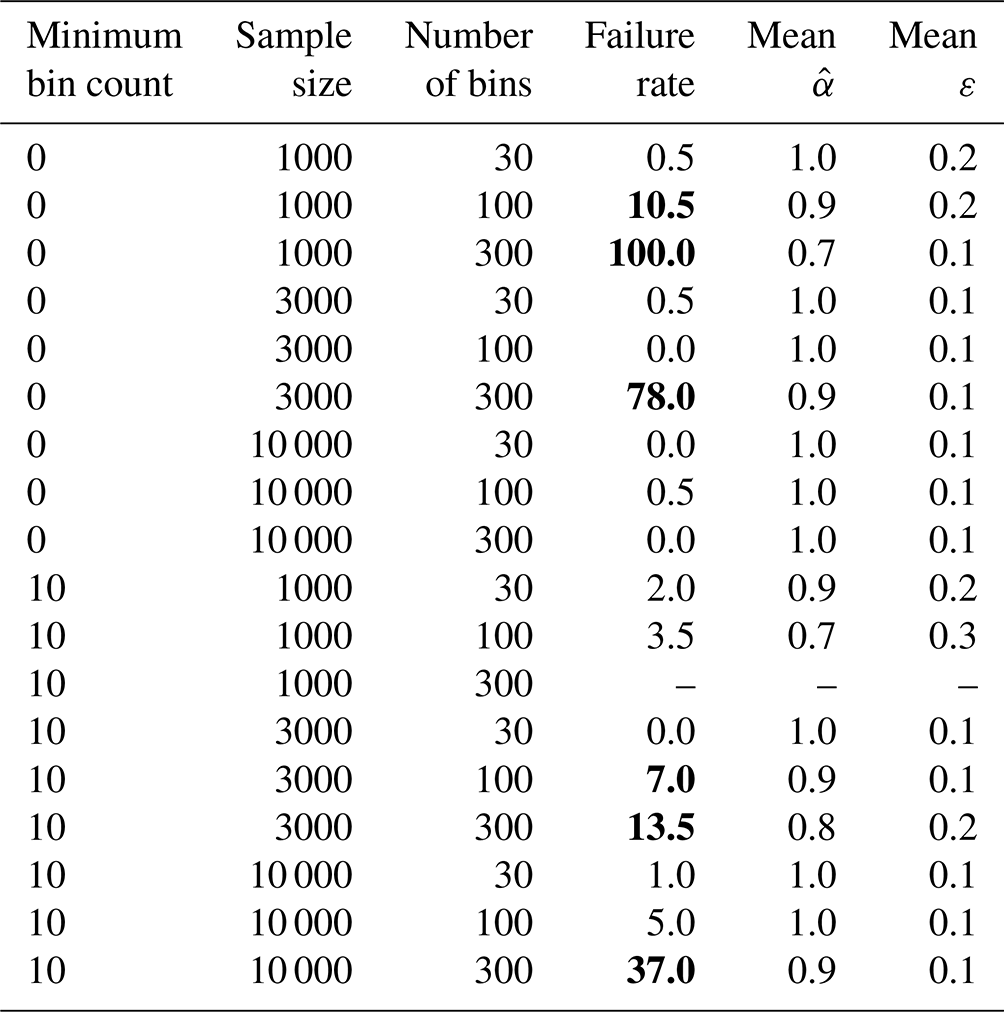
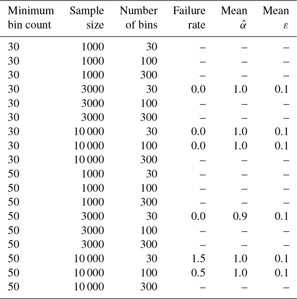
Table D2 Continuation of Table D1 for minimum bin counts of 30 and 50.