How well can persistent contrails be predicted? An update

The total aviation effective radiative forcing is dominated by non-CO₂ effects. The largest contributors to the non-CO₂ effects are contrails and contrail cirrus. There is the possibility of reducing the climate effect of aviation by avoiding flying through ice-supersaturated regions (ISSRs), where contrails can last for hours (so-called persistent contrails). Therefore, a precise prediction of the specific location and time of these regions is needed. But a prediction of the frequency and degree of ice supersaturation (ISS) on cruise altitudes is currently very challenging and associated with great uncertainties because of the strong variability in the water vapour field, the low number of humidity measurements at the air traffic altitude, and the oversimplified parameterisations of cloud physics in weather models.

Since ISS is more common in some dynamical regimes than in others, the aim of this study is to find variables/proxies that are related to the formation of ISSRs and to use these in a regression method to predict persistent contrails. To find the best-suited proxies for regressions, we use various methods of information theory. These include the log-likelihood ratios, known from Bayes' theorem, a modified form of the Kullback–Leibler divergence, and mutual information. The variables (the relative humidity with respect to ice, RHi_ERA5; the temperature, T; the vertical velocity, ω; the divergence, DIV; the relative vorticity, ζ; the potential vorticity, PV; the normalised geopotential height, Z; and the local lapse rate, γ) come from ERA5, and RH$i_{\mathrm{M}/\mathrm{I}}$, which we assume as the truth, comes from MOZAIC/IAGOS (Measurement of Ozone and Water Vapour on Airbus In-service Aircraft/In-service Aircraft for a Global Observing System; commercial aircraft measurements).

It turns out that RHi_ERA5 is the most important predictor of ice supersaturation, in spite of its weaknesses, and all other variables do not help much to achieve better results. Without RHi_ERA5, a regression to predict ISSRs is not successful. Certain modifications of RHi_ERA5 before the regression (as suggested in recent papers) do not lead to improvements of ISSR prediction. Applying a sensitivity study with artificially modified RHi_ERA5 distributions points to the origin of the problems with the regression: the conditional distributions of RHi_ERA5 (conditioned on ISS and non-ISS, from RH$i_{\mathrm{M}/\mathrm{I}}$) overlap too heavily in the range of 70 %–100 %, so for any case in that range, it is not clear whether it belongs to an ISSR or not. Evidently, this renders the prediction of contrail persistence very difficult.

1 Introduction

In order to avoid persistent (warming) contrails, it is necessary that they can be reliably predicted. For this aim, three conditions need to be fulfilled. First, the formation of contrails has to be predicted with reasonable skill. Contrails form if (super)saturation with respect to water occurs during the mixing process of the ambient air with the exhaust gases from the aircraft. This criterion is called the Schmidt–Appleman criterion (SAC; see Schmidt, 1941; Appleman, 1953; Schumann, 1996). Second, contrails need ice supersaturation (ISS) to be persistent. So, this state must be represented and reliably predicted in weather models. Third, in order to determine whether a contrail will be warming or cooling in advance, some kind of radiative transfer calculation or a corresponding regression formula (e.g. Corti and Peter, 2009; Schumann et al., 2012; Wolf et al., 2023a) is required.

While the first of these conditions, the ability to predict the SAC, is generally fulfilled with a satisfying quality, this is not the case for the prediction of ice supersaturation (Gierens et al., 2020). Predicting ice supersaturation at air traffic cruise levels presents major difficulties. Gierens et al. (2020) compared temperature and humidity data obtained from instrumented passenger aircraft with reanalysis data interpolated in space and time to the measurement locations. They came to the result that the forecast of ice supersaturation at given times and locations (for flight routing purposes) is currently almost like tossing a coin. In contrast, the forecast of ISS is much easier for larger regions and periods of time (e.g. for planning measurement campaigns; see Voigt et al., 2017). In the present paper, we investigate the problem of the forecast of ISS in more detail and we do not cover the first and third condition.

There are several reasons why the prediction of persistent contrails is currently challenging. The main reason is the strong variability in the water vapour field in the atmosphere. This is because water substance is present in three aggregate states; it is involved in chemical and aerosol processes, and thus it varies greatly in the atmosphere. This problem is intensified by the low number of humidity measurements at cruise levels for data assimilation. Data assimilation is necessary to keep the simulation of a complex system close to measured reality. Therefore, more data on relative humidity at flight levels are urgently needed. Note that satellite data cannot fill this gap since their vertical resolution is insufficient (Gierens and Eleftheratos, 2020). A third reason for the challenging prediction of persistent contrails is that current parameterisations of ice cloud physics in weather models are generally kept simple enough in order not to spend too much computing time for a part of the atmosphere that so far has usually not been the main focus of weather prediction. ISS hardly affects the weather on the ground. Thus, it was not represented in numerical weather prediction (NWP) models until about 25 years ago (Wilson and Ballard, 1999; Tompkins et al., 2007), and its representation is still generally too crude for a reliable prediction of ice supersaturation and contrail persistence.

However, there is growing interest in reducing the climate impact of aviation nowadays, and a relatively straightforward possibility would be the avoidance of the formation of persistent contrails if only ice supersaturation could be predicted with the precision necessary for flight routing. Because of the challenges mentioned before, the relative humidity field is insufficient for this purpose, and we need either corrections to the humidity field (Teoh et al., 2020, 2022) or other quantities that help in predicting of ISS. Gierens and Brinkop (2012) and Wilhelm et al. (2022) show that ISS is typically related to certain dynamical regimes, e.g. anticyclonic divergent uplift. This triggered the idea that using dynamical fields can indeed help in contrail forecast. We pursue this idea in the present study and show how far we can get with dynamical proxies together with modern regression methods. The results turn out to be considerably better than without such methods, but they are still not satisfying. A sensitivity study shows what impedes better results and where the source of the problem lies.

In the present paper, we concentrate on the prediction of ice supersaturation, i.e. the prediction of persistent contrails. For this purpose, we use data obtained from an instrumented passenger aircraft and reanalysis data, which are explained in Sect. 2. We test different methods for predicting persistent contrails, which is the content of Sect. 3, as well as the results we obtained. Later on, in Sect. 4, we concentrate on modifying the relative humidity of ERA5 and on different sensitivity tests to artificially separate the conditional RHi distributions of ERA5. Finally, we summarise our results and conclude in Sect. 5.

2 Data

Various data sources are utilised in this study. These are briefly described in the following sections, Sect. 2.1 and 2.2.

2.1 Data from a commercial aircraft

In this study, we use pressure and relative humidity with respect to ice (RH$i_{\mathrm{M}/\mathrm{I}}$) data collected from 16 588 flights during 10 years (2000–2009) of MOZAIC (Measurement of Ozone and Water Vapour on Airbus In-service Aircraft; Marenco et al., 1998) measurements. As MOZAIC was transferred to the European infrastructure IAGOS (In-service Aircraft for a Global Observing System; Petzold et al., 2015) in 2011, we refer to the data as MOZAIC/IAGOS (https://www.iagos.org, last access: 4 July 2024). MOZAIC/IAGOS operates autonomous in situ instruments installed on a long-range commercial aircraft. Due to this, it has the highest data density in the flight corridors of the mid-latitudes, making it an ideal data set for the investigation of contrail-forming regions. MOZAIC/IAGOS in situ measurements are available every 4 s. This corresponds to a flight distance of around 1 km. We randomly select only 1 % of the data points (around every 100th point) to avoid autocorrelation. This means the temporal distance is around 400 s on average.

For this study, we have chosen aerial boundaries of 30 to 70° latitude and −125 to 145° longitude at cruise levels between 310 and 190 hPa, that is, a region with heavy air traffic. We use these data as a basic truth to determine whether the formation of a persistent contrail is possible or not at a specific position and time.

2.2 Reanalysis data

In addition to the data from commercial aircraft, hourly ERA5 high-resolution realisation (HRES) reanalysis data (Hersbach et al., 2018a, b, 2020) of the relative humidity with respect to ice, RHi_ERA5; the temperature, T; the vertical velocity, ω; the divergence, DIV; the relative vorticity, ζ; the potential vorticity, PV; and the normalised geopotential height, Z, for 200, 225, 250, and 300 hPa from the Copernicus Data Service (Copernicus Climate Change Service, 2017) of ECMWF (European Centre for Medium-Range Weather Forecast) are retrieved and interpolated to the exact position and time of the aircraft (see ERA5, https://cds.climate.copernicus.eu, last access: 4 July 2024). The chosen pressure range from 300 to 200 hPa covers approximately the flight levels of 300 to 390 hft (hectofeet; 100 ft corresponds to approximately 30 m). The spatial resolution of these data is 1°×1°. With the pressure and temperatures on two adjacent levels, the local lapse rate, γ, at the aircraft positions is also calculated (Gierens et al., 2022). The selection of these particular variables comes from Wilhelm et al. (2022).

3 Methods and results

In this work, we consider whether it is possible to use the dynamical proxies suggested by Wilhelm et al. (2022) to improve the forecast of ice supersaturation and contrail persistence. To quantify the success (or not) of several approaches we took, we use the equitable thread score (ETS) as in Gierens et al. (2020). The motivation for this choice of score value, the defining equations, and interpretation of the ETS are given below in Sect. 3.2.3.

The most simple way to map the values of the six dynamical proxies to probabilities for ice supersaturation or contrail persistence is to divide the phase space into six-dimensional rectangles/blocks (six because of the six suggested dynamical proxies by Wilhelm et al., 2022), to count the number of cases with persistent contrails in each block, and to divide it by the total amount of data in that block. The blocks should not be too large so that the probabilities are specific for certain circumstances. Simultaneously, the blocks must not be too small so that the number of events in each block allows one to determine the probability with some statistical reliability. Unfortunately, it turns out that even almost 400 000 data points are insufficient for this simple and most straightforward method; many blocks are either empty or do not have enough data points unless we use quite large blocks and lose precision. Therefore, we cannot use this simple method and have to try others, like Bayesian learning or modern non-linear regression methods.

3.1 Bayesian learning

3.1.1 Theory

We are interested in whether persistent contrails are possible or not, i.e. whether there is ice supersaturation or not. Unfortunately, the moisture field in the models is not accurate enough for that purpose. So, how can we solve this problem?

It is known that ISS is more frequent in some dynamic situations than in others (Gierens and Brinkop, 2012; Gierens et al., 2022; Wilhelm et al., 2022). One can try to exploit the fact that there are certain dynamical quantities, X, whose conditional probability densities, f_X(x|ISS) and $f_X\left(x\right|\stackrel{\mathrm{‾}}{\mathrm{ISS}})$, differ more or less from each other (read as f_X(x|ISS) being the probability density for a quantity X for the special value x in cases where ISS prevails; $f_X\left(x\right|\stackrel{\mathrm{‾}}{\mathrm{ISS}})$ is the analogue for cases where non-ISS ($\stackrel{\mathrm{‾}}{\mathrm{ISS}}$) prevails).

Let us assume there is a value x of a variable X and that this particular value is compatible with both ISS and $\stackrel{\mathrm{‾}}{\mathrm{ISS}}$. Then the question arises of which statements can be made about ice supersaturation using this quantity. Is it more likely or less likely when X=x?

Naively, one could compare f_X(x|ISS) and $f_X\left(x\right|\stackrel{\mathrm{‾}}{\mathrm{ISS}})$ and choose the larger of the two values. However, this ignores the fact that $\stackrel{\mathrm{‾}}{\mathrm{ISS}}$ cases are much more frequent than ISS cases when no further circumstances are considered – the so-called a priori probability. The latter is taken into account by Bayes' theorem in the following form:

$$\begin{array}{}\text{(1)}& P\left(\mathrm{ISS}\right|X=x)={\displaystyle \frac{P\left(x\right|\mathrm{ISS})\cdot P(\mathrm{ISS})}{P\left(x\right|\mathrm{ISS})\cdot P(\mathrm{ISS})+P(x\left|\stackrel{\mathrm{‾}}{\mathrm{ISS}}\right)\cdot P\left(\stackrel{\mathrm{‾}}{\mathrm{ISS}}\right)}},\end{array}$$

where P(ISS) is the a priori probability for ice supersaturation. $P\left(x\right|\mathrm{ISS})=f_X(x\left|\mathrm{ISS}\right)\mathrm{d}x$ and $P\left(x\right|\stackrel{\mathrm{‾}}{\mathrm{ISS}})=f_X(x\left|\stackrel{\mathrm{‾}}{\mathrm{ISS}}\right)\mathrm{d}x$. In Eq. (1), the dx is cancelled out and, on the right side of the equation, P(x|ISS) and $P\left(x\right|\stackrel{\mathrm{‾}}{\mathrm{ISS}})$ can be replaced by the corresponding densities, f_X(x|ISS) and $f_X\left(x\right|\stackrel{\mathrm{‾}}{\mathrm{ISS}})$.

Another possibility of framing Bayes’ theorem for the present problem is to use an odds ratio:

$$\begin{array}{}\text{(2)}& {\displaystyle \frac{P\left(\mathrm{ISS}\right|x)}{P\left(\stackrel{\mathrm{‾}}{\mathrm{ISS}}\right|x)}}={\displaystyle \frac{f_X\left(x\right|\mathrm{ISS})}{f_X\left(x\right|\stackrel{\mathrm{‾}}{\mathrm{ISS}})}}\cdot {\displaystyle \frac{P\left(\mathrm{ISS}\right)}{P\left(\stackrel{\mathrm{‾}}{\mathrm{ISS}}\right)}}.\end{array}$$

The first factor on the right side of Eq. (2) is the likelihood ratio, which represents the gain (>1) or loss (<1) in confidence for ISS that we get by learning the current value of X. A likelihood ratio exceeding 1 does not mean that ISS is more likely than $\stackrel{\mathrm{‾}}{\mathrm{ISS}}$ but that the probability of ISS increases. ISS is only more likely than $\stackrel{\mathrm{‾}}{\mathrm{ISS}}$ if the factor on the left side, the a posteriori odds ratio, is larger than 1. The second factor on the right side is the prior odds ratio. In our case, P(ISS) is given by the ratio of the number of data points with ISS and the total number of data points (according to MOZAIC/IAGOS), which is 0.125. So, only 12.5 % of our data belong to the ISS class. The prior odds ratio is therefore $\mathrm{0.125}/\mathrm{0.875}\approx \mathrm{0.14}$. This means that the likelihood ratio has to be larger than $\mathrm{1.0}/\mathrm{0.14}=\mathrm{7.14}$ to make ISS more probable than $\stackrel{\mathrm{‾}}{\mathrm{ISS}}$. Instead of the odds ratio, one often uses its logarithm, which leads to log-likelihood ratios (also known as logits) with values symmetric around 0 (instead of values asymmetric around 1). That is, positive logits increase the probability for ISS and negative logits decrease the probability for ISS. As mentioned before, the a posteriori odds ratio has to be larger than 1 to make ISS more probable than $\stackrel{\mathrm{‾}}{\mathrm{ISS}}$. This also means that the logarithm of the a posteriori ratio has to be positive to make ISS more likely than $\stackrel{\mathrm{‾}}{\mathrm{ISS}}$. As the logarithm of the prior odds ratio is $\ln (\mathrm{0.125}/(\mathrm{1}-\mathrm{0.125}\left)\right)\approx -\mathrm{2}$, the logit must exceed 2 to make ISS more probable than $\stackrel{\mathrm{‾}}{\mathrm{ISS}}$.

As long as there is only one special value x of a dynamical variable X, we are finished and this is already the result. Now, assume that there are two quantities, X and Y, and one wants to know which of these quantities carries more information about the probability of ice supersaturation. Obviously, it is the quantity whose logits deviate more from zero in both the positive and negative directions or the quantity for which the absolute values of the logits are larger on average over the ranges of x and y. Taking the averages has to be done with a weighting that accounts for the values of the variables that actually occur in a given situation, e.g.

$$\begin{array}{}\text{(3)}& E_{\mathrm{AL}}\left(f_{X|\mathrm{ISS}}\right|\left|f_{X|\stackrel{\mathrm{‾}}{\mathrm{ISS}}}\right)=\int f_X\left(x\right|\mathrm{ISS})\cdot \left|\ln \left({\displaystyle \frac{f_X\left(x\right|\mathrm{ISS})}{f_X\left(x\right|\stackrel{\mathrm{‾}}{\mathrm{ISS}})}}\right)\right|\mathrm{d}x.\end{array}$$

As one does not know in advance whether a situation is ISS or not, it is best to also use the corresponding expectation of the absolute logit, $E_{\mathrm{AL}}\left(f_{X|\stackrel{\mathrm{‾}}{\mathrm{ISS}}}\right|\left|f_{X|\mathrm{ISS}}\right)$ (where ISS and $\stackrel{\mathrm{‾}}{\mathrm{ISS}}$ are interchanged), and to average the two results. Let the result for X be E_AL(X). It may be called the expectation of the absolute logit. The quantity that yields the largest E_AL(X) has the largest learning effect for the question of whether a situation is ISS or not.

Note that $E_{\mathrm{AL}}(.||.)$ has some resemblance to a quantity known as Kullback–Leibler divergence, $D_{\mathrm{KL}}\left(f_{X|\mathrm{ISS}}\right|\left|f_{X|\stackrel{\mathrm{‾}}{\mathrm{ISS}}}\right)$ (the same expression without the absolute sign), and the corresponding symmetric form (the mean value of the two asymmetrical divergences, $D_{\mathrm{KL}}\left(f_{X|\mathrm{ISS}}\right|\left|f_{X|\stackrel{\mathrm{‾}}{\mathrm{ISS}}}\right)$ and $D_{\mathrm{KL}}\left(f_{X|\stackrel{\mathrm{‾}}{\mathrm{ISS}}}\right|\left|f_{X|\mathrm{ISS}}\right)$) is known as Jeffreys divergence in information theory. For quantities that are not related to supersaturation, $f_X\left(x\right|\mathrm{ISS})=f_X(x\left|\stackrel{\mathrm{‾}}{\mathrm{ISS}}\right)=f_X\left(x\right)$, and the logit is zero. Thus, E_AL(X)=0 as well, which signifies that one cannot learn anything about the presence of ISS using such a quantity.

3.1.2 Application

The conditional probability densities of the dynamical proxies of ERA5 for ISS and $\stackrel{\mathrm{‾}}{\mathrm{ISS}}$ cases (depending on whether the relative humidity with respect to ice of MOZAIC/IAGOS, RH$i_{\mathrm{M}/\mathrm{I}}$, is ≥ 1.0 or <1.0) are calculated using the Epanechnikov smoothing kernel with 300 equally spaced points between the minimum and maximum of the respective proxy. The log-likelihood ratios for some dynamical quantities are shown in Fig. 1. ISS gains in probability are relative to the low prior probability if the log-likelihood ratio is positive and vice versa (solid line in the diagrams). However, it needs to exceed 2 to make ISS more probable than $\stackrel{\mathrm{‾}}{\mathrm{ISS}}$ (dashed lines). Obviously, this threshold is only exceeded in quite small ranges of the proxies or not at all. Only where RHi from ERA5 exceeds 100 % does the logit exceed 2; this says that ISS and persistent contrails are more probable than not (the wiggles in the curve at even higher RHi are considered noise). The low values of the logits of the other variables indicate that the dynamical proxies do not help much in predicting ice supersaturation via the Bayesian law. Obviously, the strong separation of their conditional distributions is only a necessary but not a sufficient condition for good proxies.

For the calculation of the expectation of the absolute logit E_AL(X) (see Eq. 3), the absolute values of the different logit functions are needed. These are shown in orange in Fig. 2 for different proxies. The products of these functions with either of the conditional densities are shown as well in light blue and dark purple. The integrals of these functions are given in Table 1 for the relative humidity with respect to ice, RHi_ERA5; the temperature, T; the vertical velocity, ω; the divergence, DIV; the relative vorticity, ζ; the potential vorticity, PV; the lapse rate, γ; and the normalised geopotential height, Z. The averages of the first two rows of each column are the desired E_AL(X). High values for RHi_ERA5, ζ, and γ are noticeable for the ISS case and high values for RHi_ERA5, PV, and γ for $\stackrel{\mathrm{‾}}{\mathrm{ISS}}$. Therefore, according to our analysis, RHi_ERA5, ζ, γ, and PV seem to be the best-suited proxies for our purpose, but, as stated, they should be tried rather for regression and not for Bayesian learning. The high value of E_AL(PV) is probably due to the fact that a high PV indicates the stratosphere where ISS hardly occurs. So, for tropospheric situations (low-PV cases), this finding is not very helpful, and, accordingly, the high E_AL(PV) must not be over-interpreted.

To apply the Bayesian law for several proxies simultaneously, e.g. as for $P\left(\mathrm{ISS}\right|\mathrm{RH}{i}_{\mathrm{ERA}\mathrm{5}},\mathit{\zeta },\mathit{\gamma })$, we would need a much larger amount of data to compute the likelihood ratios with some robustness over the whole domain. Instead, we now try to apply non-linear regression.

Table 1 Expectation values for absolute logit of the different proxies. E_AL(X) is the mean of $E_{\mathrm{AL}}\left(f_{X|\mathrm{ISS}}\right|\left|f_{X|\stackrel{\mathrm{‾}}{\mathrm{ISS}}}\right)$ and $E_{\mathrm{AL}}\left(f_{X|\stackrel{\mathrm{‾}}{\mathrm{ISS}}}\right|\left|f_{X|\mathrm{ISS}}\right)$, so $E_{\mathrm{AL}}\left(X\right)=\frac{\mathrm{1}}{\mathrm{2}}\cdot \left(E_{\mathrm{AL}}\left(f_{X|\mathrm{ISS}}\right|\left|f_{X|\stackrel{\mathrm{‾}}{\mathrm{ISS}}}\right)+E_{\mathrm{AL}}\left(f_{X|\stackrel{\mathrm{‾}}{\mathrm{ISS}}}\right|\left|f_{X|\mathrm{ISS}}\right)\right)$.

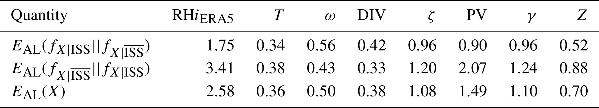
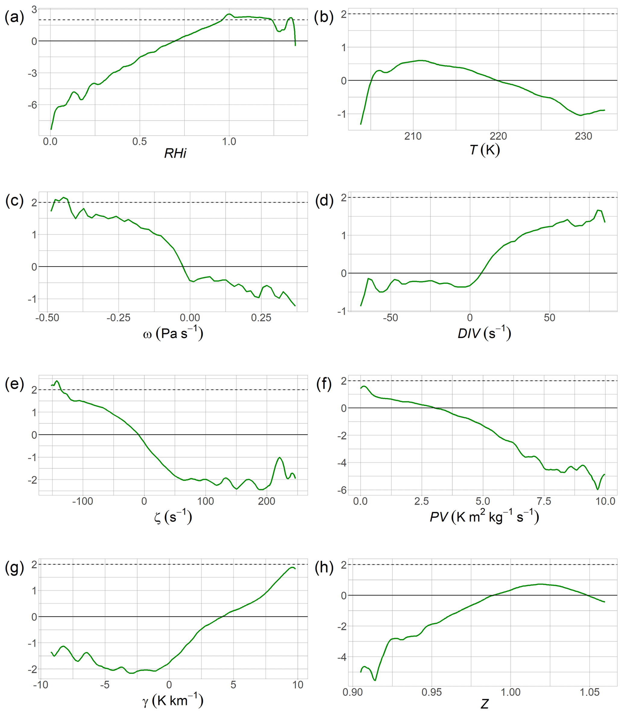
Figure 1 Log-likelihood ratios for dynamical quantities. Positive values raise the probability for ISS and negative values lower it. The probability for ISS exceeds the probability for $\stackrel{\mathrm{‾}}{\mathrm{ISS}}$ only in the small ranges where the log likelihood reaches values above 2 (marked by the dashed lines).

Figure 2 The absolute logarithm of the quotient of the densities for ISS and $\stackrel{\mathrm{‾}}{\mathrm{ISS}}$ cases (orange), the absolute logarithm of the quotient of the densities for ISS and $\stackrel{\mathrm{‾}}{\mathrm{ISS}}$ cases multiplied by the density for ISS cases (light blue), and the absolute logarithm of the quotient of the densities for $\stackrel{\mathrm{‾}}{\mathrm{ISS}}$ and ISS cases multiplied by the density for $\stackrel{\mathrm{‾}}{\mathrm{ISS}}$ cases (dark purple) (see Eq. 3).

3.2 Non-linear regression

The dynamical candidate proxies are not independent quantities, and one has to take care that a regression is not formulated with redundant information. But, of course, a variable that has some relation with (i.e. information on) the relative humidity is welcome. Above, we see that RHi_ERA5, ζ, and γ are promising in this respect. Also, PV has a quite large absolute logit, but that comes mainly from the $\stackrel{\mathrm{‾}}{\mathrm{ISS}}$ cases, where it is an expression of the fact that dry stratospheric air (with PV>3.5) is rarely found in a supersaturated state (Neis, 2017; Petzold et al., 2020). Here, we apply another measure. Usually, one uses the linear correlation between the input data, but this does not work if the quantities are related in a non-linear fashion. Therefore, it is necessary to use a more general measure of correlation, namely the mutual information from information theory.

3.2.1 Mutual information

The mutual information is a measure of information that one variable, X, can provide about another, Y. Its formulation uses the joint distribution of X and Y and both marginal distributions:

$$\begin{array}{}\text{(4)}& I(X;Y)=\int \int f_{X\cap Y}(x,y)\cdot \log \left({\displaystyle \frac{f_{X\cap Y}(x,y)}{f_X\left(x\right)\cdot f_Y\left(y\right)}}\right)\mathrm{d}x\mathrm{d}y,\end{array}$$

where $f_{X\cap Y}(x,y)$ is the joint probability density for X and Y. In the case that X and Y are independent, the joint density equals the product of the marginal densities and the logarithm is zero. Then, the mutual information between X and Y is zero as well. In all other cases, it is positive and it is the expected value of $\log \left(\frac{f_{X\cap Y}}{f_X{f}_Y}\right)$ with the joint distribution as the weight function.

Since we assume the humidity of MOZAIC/IAGOS (RH$i_{\mathrm{M}/\mathrm{I}}$) is the truth, we calculate the mutual information of RH$i_{\mathrm{M}/\mathrm{I}}$ with other quantities and compare them with each other. The results of the computed mutual information $I(\mathrm{RH}{i}_{\mathrm{M}/\mathrm{I}};Y)$ for different variables Y are shown in the first row in Table 2. The highest values of the mutual information are reached by RHi_ERA5 (1.26 bits), PV (0.57 bits), γ (0.38 bits), and ζ (0.37 bits). This means, according to the mutual information, that RHi_ERA5, PV, γ, and ζ seem well suited as proxies for regressions.

To be a good proxy for a regression, it must not only be well correlated with RH$i_{\mathrm{M}/\mathrm{I}}$ (i.e. have a high value of mutual information, $I(\mathrm{RH}{i}_{\mathrm{M}/\mathrm{I}};Y)$, but, at the same time, it should not be correlated with other variables (i.e. a low value of mutual information with the other proxies, I(X;Y)) to avoid redundant information. The values of the individual mutual information, I(X;Y), can be found on the right side in Table 2. The matrix is symmetrical, so, for a better overview, only one side is filled.

As mentioned before, out of all quantities, RHi_ERA5, PV, γ, and ζ have the highest mutual information with RH$i_{\mathrm{M}/\mathrm{I}}$. However, PV and γ are themselves quite strongly correlated (1.07 bits). So, because $I(\mathrm{RH}{i}_{\mathrm{M}/\mathrm{I}};\mathrm{PV})>I(\mathrm{RH}{i}_{\mathrm{M}/\mathrm{I}};\mathit{\zeta })$ but I(PV;ζ) is also very high, ζ should be omitted when using PV as a proxy.

Table 2 The mutual information matrix, I(X;Y), is used to identify the correlations of the variables with each other. The first row of the matrix, $I(\mathrm{RH}{i}_{\mathrm{M}/\mathrm{I}};Y)$, shows the correlation of RH$i_{\mathrm{M}/\mathrm{I}}$ with the other proxies and the columns the correlations between the variables among themselves.

3.2.2 Generalised additive model

A generalised additive model (GAM) is a regression method for predicting a response Y based on non-linear functions of several predictors, $X=\mathit{\{}{X}_{\mathrm{1}},X_{\mathrm{2}},\mathrm{\dots },X_{\mathrm{p}}\mathit{\}}$. In meteorology, for instance, it has been successfully used for the prediction of thunderstorms (Rädler et al., 2018). The general formula for GAMs is

$$\begin{array}{}\text{(5)}& \log \left({\displaystyle \frac{P\left(\mathrm{ISS}\right|X)}{\mathrm{1}-P\left(\mathrm{ISS}\right|X)}}\right)={\mathit{\beta }}_{\mathrm{0}}+s_{\mathrm{1}}\left(X_{\mathrm{1}}\right)+s_{\mathrm{2}}\left(X_{\mathrm{2}}\right)+\mathrm{\dots }+s_{\mathrm{p}}\left(X_{\mathrm{p}}\right).\end{array}$$

$\frac{P\left(\mathrm{ISS}\right|X)}{\mathrm{1}-P\left(\mathrm{ISS}\right|X)}$ is the posterior odds ratio, P(ISS|X)/$P\left(\stackrel{\mathrm{‾}}{\mathrm{ISS}}\right|X)$. The GAM thus constructs a relation between the (posterior) odds ratio and a linear combination of functions of the set of predictors, X. For the functions, we use smoothing splines, s(X). Here, we test the following six different GAMs with combinations of various dynamical proxies (input parameters) to predict whether persistent contrails are possible:

• GAM₀ with RHi_ERA5,

• GAM₁ with T, RHi_ERA5,

• GAM₂ with PV, T, RHi_ERA5,

• GAM₃ with PV, T, ζ, RHi_ERA5,

• GAM₄ with γ, T, Z, PV, ζ, and

• GAM₅ with γ, T, Z, PV, ζ, RHi_ERA5 .

The procedure is as follows: for the tests, 395 576 independent data points are used. First, we divide the data set (MOZAIC/IAGOS and ERA5 data) into a training and test data set (training data set makes up ∼ 80 % and test data set ∼ 20 % of the whole data set). The presence of persistent contrails is known from the MOZAIC/IAGOS data, as described in Sect. 2.1. Next, we train the model, which means that we find the best coefficients for the relationships between the proxies and prediction using the training data set and a software environment for statistical computing called R (Ihaka and Gentleman, 1993). Then, we use the gained best coefficients and functions to predict the presence of persistent contrails in the test data set. At the end, we validate the forecast by comparing the predictions with the truth and calculating the so-called equitable threat score (see Sect. 3.2.3).

3.2.3 Equitable threat score

In this study, the equitable threat score (ETS) is used to validate and compare the prediction accuracy of the different GAMs (with varied input parameters) with that of the raw data. For the calculation of the ETS (Gierens et al., 2020), the events are summed up according to the contingency table (see Table 3), where a distinction is made between potential persistent contrails predicted (yes or no) and persistent contrails observed (yes or no).

Table 3 Contingency table for predicting and observing persistent contrails.

The sum of the events is labelled as a (contrails are predicted and observed), b (no contrails are predicted but observed), c (contrails are predicted but not observed), and d (contrails are neither predicted nor observed). For the calculation of the ETS, the numbers of the events, a, b, c, and d, and the following equation are used:

$$\begin{array}{}\text{(6)}& \mathrm{ETS}={\displaystyle \frac{a-r}{a+b+c-r}},\end{array}$$

with

$$\begin{array}{}\text{(7)}& r={\displaystyle \frac{(a+b)\cdot (a+c)}{a+b+c+d}}.\end{array}$$

If the prediction agrees perfectly with the observation, ETS =1. For a completely inverse relation, ETS is negative, and for a random relation, ETS=0. The advantage of using ETS instead of another skill score is that the influence of the predominant case in which ISS is neither predicted nor observed (large value of d) is minimised. This is the case here, since $\stackrel{\mathrm{‾}}{\mathrm{ISS}}$ is much more probable than ISS.

In order to fill the contingency table, it is necessary to decide on a conditional probability threshold P(ISS|X) up to which $\stackrel{\mathrm{‾}}{\mathrm{ISS}}$ and from which ISS is predicted. To determine the threshold, one generally uses the value that gives the best ETS. In the present case, this threshold probability is 0.34. That is, with a given set of proxies, X, we predict contrail persistence or ice supersaturation if $P\left(\mathrm{ISS}\right|X)>\mathrm{0.34}$ (and vice versa).

3.2.4 Regression results

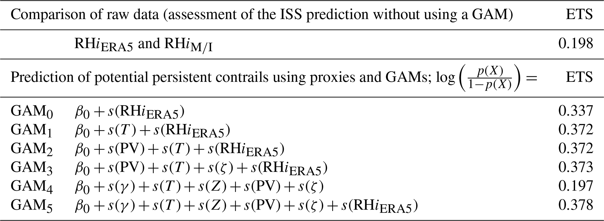
Table 4 shows the results of the application of six different general additive models (GAM₀ to GAM₅). Note that β₀ is different for every GAM even if it is abbreviated in the same way in all GAMs. In the first (white) row, the ETS value of 0.198 is given, which is obtained when only RHi_ERA5 and RH$i_{\mathrm{M}/\mathrm{I}}$ are compared (without applying a GAM to it). In that case, we only check how well the prediction of ISS in ERA5 matches the observation of ISS of MOZAIC/IAGOS. So, it is only examined how often RHi_ERA5 ≥ 1.0 matches RH$i_{\mathrm{M}/\mathrm{I}}$ ≥ 1.0. The SAC is not taken into account.

In GAM₀, we only use RHi_ERA5 and get an ETS value of 0.337. In GAM₁, we also take T into account since the temperature and the humidity are the two important variables to compute whether contrails form (using the SAC). With these proxies we get an ETS of 0.372, which is a little bit higher than in GAM₀ but not significantly.

As we saw in Sect. 3.2.1, when calculating the mutual information, RHi_ERA5, PV, ζ, and γ show particularly high values with RH$i_{\mathrm{M}/\mathrm{I}}$ ($I(\mathrm{RH}{i}_{\mathrm{M}/\mathrm{I}};\mathrm{RH}{i}_{\mathrm{ERA}\mathrm{5}})$ =1.26 bits, $I(\mathrm{RH}{i}_{\mathrm{M}/\mathrm{I}};\mathrm{PV})$ =0.57 bits, $I(\mathrm{RH}{i}_{\mathrm{M}/\mathrm{I}};\mathit{\gamma })$ =0.38 bits, and $I(\mathrm{RH}{i}_{\mathrm{M}/\mathrm{I}};\mathit{\zeta })$ =0.37 bits) and are therefore very suitable as proxies. But when looking at the mutual information among these proxies, then it is noticeable that in particular PV and γ correlate strongly (1.07 bits). That is why γ can be omitted when using PV. I(PV;ζ) is also very high (0.73 bits), which is why we only use the PV in GAM₂ (in addition to T and RHi_ERA5). The resulting ETS value is also 0.372.

For GAM₃, we use PV, T, ζ, and RHi_ERA5 because we want to enter even more proxies in the GAM as inputs according to the mutual information. So, we do the same GAM as before, but we also use ζ because $I(\mathrm{RH}{i}_{\mathrm{M}/\mathrm{I}};\mathit{\zeta })$ is also very high and $I(\mathrm{PV};\mathit{\zeta })<I(\mathrm{PV};\mathit{\gamma })$. The ETS in this case is 0.373. We see that GAM₂ and GAM₃ hardly differ from GAM₁ in terms of their ETS values. The reason for this is that even if $I(\mathrm{RH}{i}_{\mathrm{M}/\mathrm{I}};\mathrm{PV})$ is very high, the PV is already very strongly correlated with RHi_ERA5 ($I(\mathrm{RH}{i}_{\mathrm{ERA}\mathrm{5}};\mathrm{PV})=\mathrm{0.61}$ bits). This means that not much more additional information is provided by PV (and the other variables provide even less).

Next, we use all proxies that show separate distributions in their probability density functions (PDFs, not shown), P(X|ISS) vs. $P\left(X\right|\stackrel{\mathrm{‾}}{\mathrm{ISS}})$, but, as an experiment, we omit RHi_ERA5 in GAM₄. So, we use γ, T, Z, PV, and ζ as inputs. The ETS only reaches a value of 0.197. This shows us two important things:

• i.

  Even if we supposedly put more information into the GAM using more proxies, the ETS does not increase.

• ii.

  The relative humidity cannot be ignored as an input variable. This indicates that even if the relative humidity is an imprecise variable, it must not be excluded; otherwise, the ETS value will drastically decrease.

These two new insights may be explained by the log-likelihood ratios (Fig. 1): only RHi_ERA5 shows values above 2 for a large range, so ISS is more probable in this range. This is probably the reason why RHi_ERA5 has to be used as an input for the GAMs. All other quantities show values above 2 either not at all or only for a very small range.

Using the same proxies as before and adding RHi_ERA5 (GAM₅), the corresponding ETS reaches a value of 0.378.

It seems that the use of dynamical proxies in the GAMs does not outperform a simple GAM that uses only relative humidity and temperature by much. At least the ETS values obtained via the GAMs (that is, for prediction of potential persistent contrails) distinctively exceed those obtained from a simple check of the ISS prediction, as can be seen from the study of Gierens et al. (2020, in which ETS=0.08 for a relatively small set of data from 2014) and from the present much larger data set (ETS=0.198). This means that even if a value of 0.378 seems small at first glance, it is still larger than if the prediction of ice supersaturation is purely based on the relative humidity with respect to ice from the ERA5 data.

Note that despite T not being particularly prominent in neither the E_AL nor its mutual information with RH$i_{\mathrm{M}/\mathrm{I}}$, we use it in GAM₁ to GAM₅ because it is such an important quantity in the SAC, and we use the proxies to provide further information (in addition to T and RHi_ERA5). So, when running our best GAM (GAM₅), but this time without T, the ETS reaches a value of 0.357. T does not increase the ETS significantly, but we leave it in for the reasons mentioned above.

Since, as we have seen, the relative humidity should definitely be used as an input for a GAM, although it is not very precise, the questions arise of whether it is possible to improve the regression results using corrections to the relative humidity field from the weather forecast models and what the reason for why even the most advanced regression methods are not able to yield better ETS values is. These questions are dealt with in the next section.

Table 4 Results of comparing RHi_ERA5 and RH$i_{\mathrm{M}/\mathrm{I}}$ with each other and of different GAMs.

4 Sensitivity tests

If weather forecasts were perfect, contrail persistence could easily be predicted using temperature and relative humidity alone and it would not be necessary to use any proxies. Unfortunately, it seems that the predicted humidity field in particular (at least from ERA5 but certainly from other weather models as well) is not good enough to allow for such a forecast for single flights, that is, waypoint to waypoint (Gierens et al., 2020). There are plausible reasons for this, a lack of in situ observations of humidity at cruise levels and outdated cirrus parameterisations in numerical weather prediction models in particular (Sperber and Gierens, 2023). In the following, we perform regression tests with artificially changed distributions of relative humidity. We first assume that the two conditional RHi_ERA5 distributions, P(RHi_ERA5|ISS) and $P\left(\mathrm{RH}{i}_{\mathrm{ERA}\mathrm{5}}\right|\stackrel{\mathrm{‾}}{\mathrm{ISS}})$, were more separated (less overlap) than they are (ideally the overlap should be very small, including only sublimating contrails in the ISS-conditioned PDF and cases that are supersaturated but too warm in the $\stackrel{\mathrm{‾}}{\mathrm{ISS}}$-conditioned PDF). Second, we test two different methods of humidity corrections to see whether they help to reach higher ETS values in the regression models.

4.1 Separating the probability density functions conditioned on persistence

We guess that the root of the problem of predicting ice supersaturation and contrail persistence is the too strong of an overlap of the two conditional humidity PDFs, namely $f_{\mathrm{RH}{i}_{\mathrm{ERA}\mathrm{5}}}\left(r\right|\mathrm{ISS})$ and $f_{\mathrm{RH}{i}_{\mathrm{ERA}\mathrm{5}}}\left(r\right|\stackrel{\mathrm{‾}}{\mathrm{ISS}})$, where r is a special value of RHi_ERA5. This substantial overlap can be seen in panel (f) of Fig. 3. Now we artificially separate these two distributions using a perfectly separated pair of distributions, a log-normal distribution f_PC, cut off at 0.8 and 1.5 for cases that allow for persistent contrails (PC), and a second one, f_noPC, ranging from 0.0 and 0.8 for cases that do not (no PC). Then, we mix the original conditional probability distributions of all data, both in the training and test data set, more and more into the artificial distributions, namely using a weighting factor, $\mathrm{0}\le a\le \mathrm{1}$, as follows:

$$\begin{array}{}\text{(8)}& \begin{array}{rl}& f\left(r\right|\stackrel{\mathrm{‾}}{\mathrm{ISS}},a)=a{f}_{\mathrm{noPC}}+(\mathrm{1}-a\left)f_{\mathrm{RH}{i}_{\mathrm{ERA}\mathrm{5}}}\right(r\left|\stackrel{\mathrm{‾}}{\mathrm{ISS}}\right),\\ & f\left(r\right|\mathrm{ISS},a)=a{f}_{\mathrm{PC}}+(\mathrm{1}-a\left)f_{\mathrm{RH}{i}_{\mathrm{ERA}\mathrm{5}}}\right(r\left|\mathrm{ISS}\right).\end{array}\end{array}$$

Some examples of these artificial distributions are shown in Fig. 3. From these distributions, we draw random humidity values and replace the original ones with them, keeping their ISS and $\stackrel{\mathrm{‾}}{\mathrm{ISS}}$ label (i.e. either persistent contrail, RHi_a, drawn from $f\left(r\right|\mathrm{ISS},a)$ or non-persistent or no contrail drawn from $f\left(r\right|\stackrel{\mathrm{‾}}{\mathrm{ISS}},a)$). This data set is then again divided into a training (80 %) and test data (20 %) set and GAMs (with T and RHi_a like in GAM₁) and the corresponding ETSs are computed for every value of a.

The results are shown in Table 5. It is noticeable that even with a small shift in the relative humidity data, the ETS value increases drastically. This can be observed especially for small values of a, which means that if the original RHi_ERA5 data were just slightly more separated, the results would drastically improve. This is good news since it shows that the model prediction of RHi_ERA5 does not need to be perfect. Very good ETS values already appear for conditional distributions that are a little less separated than they actually are. Note that the further increase in ETS of a>0.5 is quite weak since ETS (a=0.5) already exceeds 0.9.

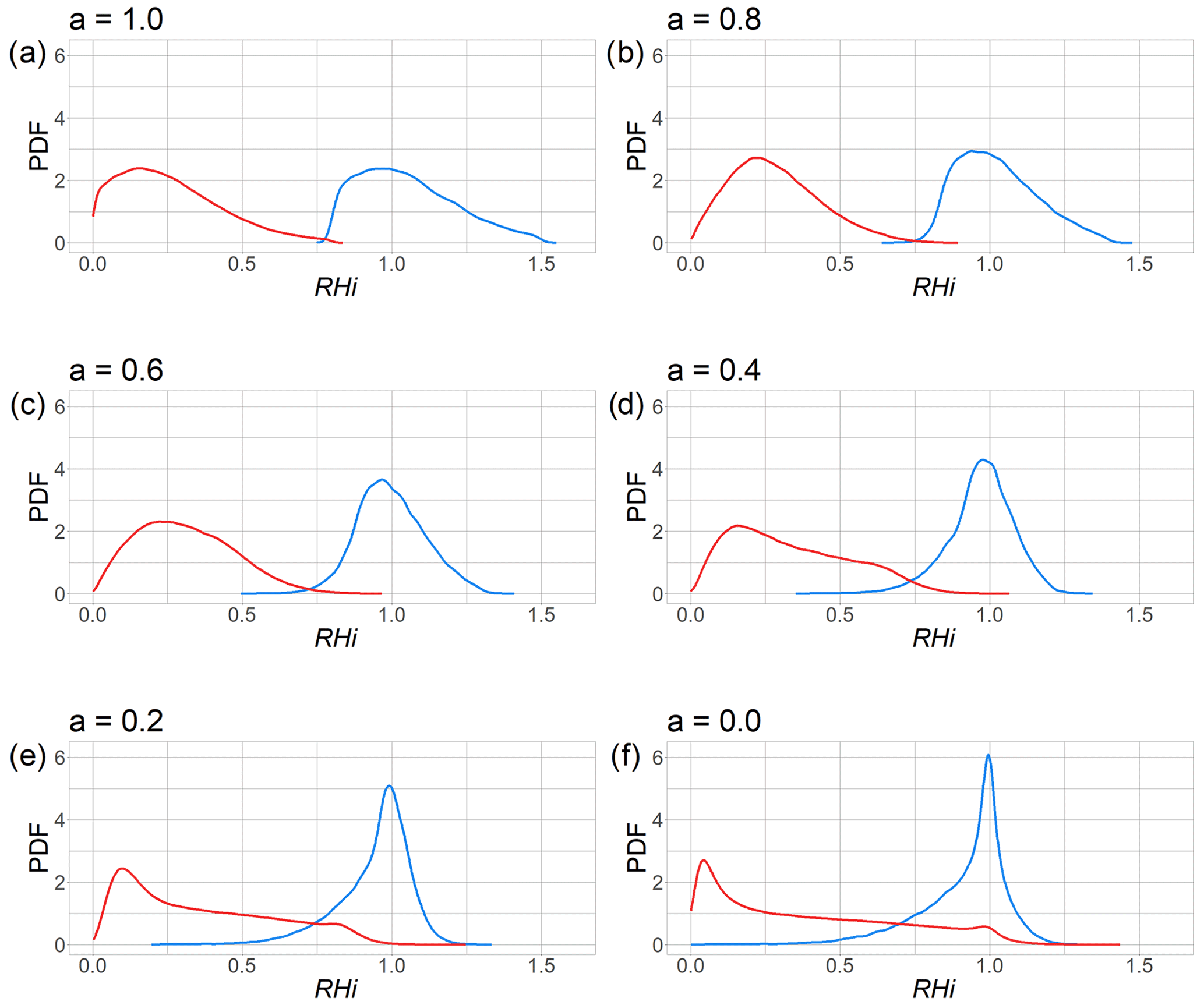
Figure 3 Conditional probability density functions $f\left(r\right|\mathrm{ISS},a)$ (blue) and $f\left(r\right|\stackrel{\mathrm{‾}}{\mathrm{ISS}},a)$ (red) for different values of a. Note that the original distributions $f_{\mathrm{RH}{i}_{\mathrm{ERA}\mathrm{5}}}\left(r\right|\stackrel{\mathrm{‾}}{\mathrm{ISS}})$ and $f_{\mathrm{RH}{i}_{\mathrm{ERA}\mathrm{5}}}\left(r\right|ISS)$ are retained with a=0.0 in panel (f).

Table 5 Results of the sensitivity test.

4.2 Correction formulas

As Sect. 4.1 shows, there is a strong increase in the ETS for decreasing overlap. For this reason, two different methods are being tested to further separate the two conditional distributions, $f_{\mathrm{RH}{i}_{\mathrm{ERA}\mathrm{5}}}\left(r\right|\mathrm{ISS})$ and $f_{\mathrm{RH}{i}_{\mathrm{ERA}\mathrm{5}}}\left(r\right|\stackrel{\mathrm{‾}}{\mathrm{ISS}})$, using corrections to the modelled relative humidity values. These correction methods are quantile mapping based on the present data sets (e.g. Gierens and Eleftheratos, 2017; Wolf et al., 2023b) and the RHi modification used by Teoh et al. (2022).

4.2.1 Quantile mapping

The quantile mapping procedure uses the two cumulative distributions of RHi, the one from the MOZAIC/IAGOS data and the corresponding one from ERA5; see Fig. 4. Evidently, the two distributions differ, in particular around saturation. This is, therefore, the range of values where corrections have the greatest effect. The procedure is quite simple: for each RHi_ERA5, the corresponding quantile value (the value on the y axis) is looked up and the corresponding RH$i_{\mathrm{M}/\mathrm{I}}$ that has the same quantile value is taken as the corrected RHi_QM. This is illustrated by the black arrows in Fig. 4. We note that saturation (RHi_QM=1) is already reached at the predicted (i.e. ERA5) relative humidity of RHi_ERA5=0.934 using this method.

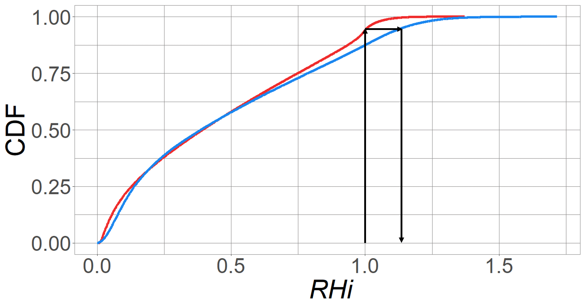
Figure 4 Illustration of quantile mapping for RHi_ERA5. The red curve illustrates the cumulative distribution function (CDF) of RHi_ERA5 and the blue one the CDF of RH$i_{\mathrm{M}/\mathrm{I}}$.

4.2.2 RHi modification by Teoh et al. (2022)

In a study by Teoh et al. (2022), the ERA5 ice supersaturation over the North Atlantic was adjusted to the corresponding MOZAIC/IAGOS supersaturation by introducing two factors used to scale RHi_ERA5:

$$\begin{array}{}\text{(9)}& \begin{array}{rl}& \mathrm{RH}{i}_{\mathrm{TEOH}}={\displaystyle \frac{\mathrm{RH}{i}_{\mathrm{ERA}\mathrm{5}}}{a}}\mathrm{if}{\displaystyle \frac{\mathrm{RH}{i}_{\mathrm{ERA}\mathrm{5}}}{a}}\le \mathrm{1},\\ & \mathrm{RH}{i}_{\mathrm{TEOH}}=min\left[{\left({\displaystyle \frac{\mathrm{RH}{i}_{\mathrm{ERA}\mathrm{5}}}{a}}\right)}^b,\mathrm{1.65}\right]\mathrm{if}{\displaystyle \frac{\mathrm{RH}{i}_{\mathrm{ERA}\mathrm{5}}}{a}}>\mathrm{1},\end{array}\end{array}$$

with a=0.9779 and b=1.635. Here we test whether this modification can lead to improvements in our regression models.

4.2.3 Results using corrections

Table 6 shows the results of comparing the observed ice supersaturation RH$i_{\mathrm{M}/\mathrm{I}}$ with the modified relative humidities with respect to ice, RHi_QM and RHi_TEOH, and the results of using these corrected humidities in the best GAM we have found before (see Sect. 3.2.4). To recall the results to be compared, which we have already described, the ETS of the comparison of RHi_ERA5 and RH$i_{\mathrm{M}/\mathrm{I}}$ and also the original GAM₅ have been added to the table.

We check how good the prediction of ice supersaturation is using the corrected versions of RHi_ERA5. When comparing the data of RH$i_{\mathrm{M}/\mathrm{I}}$ with the modified relative humidity with respect to ice using the quantile mapping method, RHi_QM, the ETS reaches a value of 0.344. If the relative humidity with respect to ice is modified according to the formula of Teoh RHi_TEOH and compared to RH$i_{\mathrm{M}/\mathrm{I}}$, then the ETS is 0.284.

Table 6 Results of comparing RH$i_{\mathrm{M}/\mathrm{I}}$ and the modified humidities, RHi_QM and RHi_TEOH, and of GAMs using RHi_QM and RHi_TEOH.

Now, we use the same proxies as in GAM₅ but we replace RHi_ERA5 with RHi_QM gained by quantile mapping and for the other case with RHi_TEOH using the formula by Teoh. The relative humidity of the whole data set is adapted. When RHi_ERA5 is modified by quantile mapping, we get an ETS value of 0.377, and for a change in humidity, according to Teoh, the ETS value is 0.376.

Unfortunately, it turns out that neither a GAM produced with quantile-mapped ERA5 humidity values nor a GAM where the Teoh et al. (2022) corrections have been applied leads to larger ETS values than a GAM without the corrections (reminder that the ETS of the original GAM₅ with the original RHi_ERA5 is 0.378). In comparison to the ETS of 0.344 (quantile mapping) and 0.284 (Teoh) mentioned above, when only the modified humidities are compared with RH$i_{\mathrm{M}/\mathrm{I}}$, the GAMs with the best-suited proxies and the modified humidities hardly affect the ETS values.

The probable reason for this negative result is seen in Fig. 5, which shows the original conditional PDFs (red and blue) together with those obtained when the corrections are applied. Evidently, there is some shift for the PDFs conditioned on ISS in particular, but the overlap between the distribution pairs still remains considerable, that is, too substantial for a better result.

Another reason for the insensitivity of the GAMs to these corrections may be that they absorb such modifications in the coefficients of the non-linear smooth functions. This may become clearer if one thinks of a linear regression ($Y={\mathit{\beta }}_{\mathrm{0}}+{\mathit{\beta }}_{\mathrm{1}}X+\mathit{\epsilon }$) where a linear correction of the predictor X, that is, $X^{\prime }=a+bX$, would also simply be absorbed in the regression coefficients β₀ and β₁. That is, they would simply take different values, but the form of the regression and the ETS would not change.

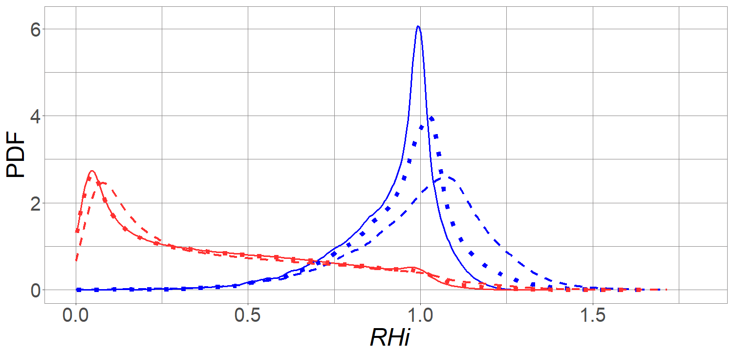
Figure 5 The conditioned PDFs P(RHi|ISS) (blue) and $P\left(\mathrm{RH}i\right|\stackrel{\mathrm{‾}}{\mathrm{ISS}})$ (red) of different RHi distributions are shown. The solid curves are the PDFs of the original RHi_ERA5 of the whole data set for $\stackrel{\mathrm{‾}}{\mathrm{ISS}}$ and ISS. The other curves represent RHi corrections: the dashed lines are the conditioned PDFs of RHi_QM modified by the quantile mapping method. The dotted curves represent the conditioned PDFs of RHi_TEOH modified by the Teoh formula.

5 Summary and conclusions

There are various approaches to minimising the climate impact of aviation. One of these approaches is to prevent the formation of persistent contrails by avoiding flying through ice-supersaturated regions, where contrails can last for hours. For implementing such aircraft diversions, these regions have to be accurately predicted in terms of time and location, which is currently associated with difficulties and uncertainties. This is mainly due to the inaccurate forecast of the relative humidity. Since ice supersaturation (ISS) is more common in some dynamical regimes than in others, we use different dynamical proxies (in addition to the relative humidity with respect to ice RHi_ERA5 and to the temperature T) as inputs to various approaches and methods to improve the prediction of these regions. These methods include a Bayesian approach and different regression models. The data of the variables/proxies come from ERA5, and the observation comes from MOZAIC/IAGOS, which we assume as the truth. With the data of MOZAIC/IAGOS, we can make the distinction between ISS and $\stackrel{\mathrm{‾}}{\mathrm{ISS}}$. The evaluation of the different methods is carried out with a score value (ETS) that checks how well the prediction matches the observation.

To find out which dynamical variables are best suited for the regressions and which do not provide redundant information, we use various methods of information theory and test them. These include the log-likelihood ratios, known from Bayes' theorem; a modified form of the Kullback–Leibler divergence, which we call the expectation of the absolute logit; and the mutual information.

Log-likelihood ratios with values greater than 2 indicate that ISS is more likely than $\stackrel{\mathrm{‾}}{\mathrm{ISS}}$. Only RHi_ERA5 delivers values above 2 in a larger range, which indicates that ISS is more likely there than $\stackrel{\mathrm{‾}}{\mathrm{ISS}}$. The vertical velocity, ω, and the relative vorticity, ζ, also show values above 2 but in a very small range. All other log-likelihood ratios are always below 2, which means that their effect on updating the prior odds ratio is quite small.

Particularly high values of the expectation for absolute logits are found for RHi_ERA5; the lapse rate, γ; and the relative vorticity, ζ, which means that these proxies have the greatest learning effect when assessing whether the situation is ISS or $\stackrel{\mathrm{‾}}{\mathrm{ISS}}$.

Furthermore, to estimate the suitability of a proxy for a regression, we use the mutual information, which is a measure of how much information one variable, X, can provide about another variable, Y. To be a good predictor of ISS, it is important that the variable is both very well correlated with the relative humidity of the MOZAIC/IAGOS data, RH$i_{\mathrm{M}/\mathrm{I}}$ (which we assume as the truth), and at the same time as uncorrelated as possible with the other variables. RHi_ERA5, PV, γ, and ζ have the highest mutual information on RH$i_{\mathrm{M}/\mathrm{I}}$, but PV and γ are themselves especially quite strongly correlated, so it is sufficient for a regression to use PV and omit γ because of the higher mutual information of PV with RH$i_{\mathrm{M}/\mathrm{I}}$.

We use the most promising variables in several regression models to predict ISS. Through the regressions we find out that no matter which and how many dynamical proxies are added as an input, they provide only little new information regarding ISS. With only the raw RHi_ERA5 and T data of ERA5, Gierens et al. (2020) could achieve an ETS value of 0.08 for the prediction of ice supersaturation. For the present data set, it is 0.198. The best regression that we can find achieves an ETS of 0.378. We consider this not satisfying for flight routing.

It turns out that the dynamical proxies hardly provide information on the question of whether a situation is ISS or $\stackrel{\mathrm{‾}}{\mathrm{ISS}}$, although the mutual information between RHi_ERA5 and RH$i_{\mathrm{M}/\mathrm{I}}$ and between PV and RH$i_{\mathrm{M}/\mathrm{I}}$ in particular is quite large. Furthermore, we see that, of all variables, only RHi_ERA5 has a range of values with the logit function exceeding the critical level of 2 and that a regression without RHi_ERA5 is not successful. Thus, it turns out that the relative humidity, RHi_ERA5, at flight level is essential in our regressions in spite of its weaknesses. We suspect that the main problem with predicting ISS is the strong overlap of the conditional probability density functions P(RHi_ERA5|ISS) and $P\left(\mathrm{RH}{i}_{\mathrm{ERA}\mathrm{5}}\right|\stackrel{\mathrm{‾}}{\mathrm{ISS}})$, especially in the critical region around RHi_ERA5 of 70 % to 100 %. Sensitivity tests show that the ETS increases strongly with a decrease in the overlap, which means that if P(RHi_ERA5|ISS) and $P\left(\mathrm{RH}{i}_{\mathrm{ERA}\mathrm{5}}\right|\stackrel{\mathrm{‾}}{\mathrm{ISS}})$ were just slightly more separated, the results would drastically improve. While corrections of RHi_ERA5 lead to better predictions of ice supersaturation (increase in the ETS values) for comparing RH$i_{\mathrm{M}/\mathrm{I}}$ with the modified relative humidities, they only slightly improve the forecast of potential persistent contrails (based on the ETS of the ISS prediction) using regression methods, the proxies that turned out to be the most suitable ones, and the modified relative humidities. This is due to the fact that the overlap of the conditional PDFs P(RHi|ISS) and $P\left(\mathrm{RH}i\right|\stackrel{\mathrm{‾}}{\mathrm{ISS}})$ of the modified relative humidities is also hardly reduced and probably also because the corrections are absorbed by the regressions, and thus they do not become effective.

In the present paper, we use the meteorological data only at the point and time where the prediction of ice supersaturation is required. One can increase the effort and use additional forecast data from earlier points in time and locations upstream of the location of interest (e.g. Duda and Minnis, 2009a, b). Wang et al. (2024) report that the humidity forecast of the ECMWF model can be improved by the application of an artificial neural network fed with data from previous atmospheric states (a couple of hours) and covering about 100 hPa in vertical distance in order to account for the past vertical motion that led to the current state. While this is certainly a possibility when it comes to improving the predicted humidity field per se, it is not clear whether the methods are fast and accurate enough for flight planning. Duda and Minnis (2009b) conclude that “reductions in the uncertainties of meteorological variables to a point where acceptable contrail forecasts are produced would be a good goal for NWA [numerical weather analysis] modelers”.

We conclude that the representation of RHi in models of numerical weather prediction needs to be improved. There are several ways to do this, but it will take some time to realise any of them. Cloud physics in numerical weather models is greatly simplified. This was justified for a long time because of the constraints of computing time and because the processes at flight level were not the focus of weather prediction. However, as aviation needs to reduce its climate impact, avoidance of contrails gets interesting for airlines and thus the prediction of ice supersaturation needs improvement. Furthermore, computer power is rising and additional resources can be used to improve the description of physical processes. A recent example is the concept of a one-moment scheme by Sperber and Gierens (2023). Furthermore, we think that more aircraft need to be equipped with hygrometers to measure humidity at flight altitudes for data assimilation. This would enable numerical weather models to improve the prediction of relative humidity for flight routing.