Diagnosing ozone–NO_x–VOC–aerosol sensitivity and uncovering causes of urban–nonurban discrepancies in Shandong, China, using transformer-based estimations

Narrowing surface ozone disparities between urban and nonurban areas escalate health risks in densely populated urban zones. A comprehensive understanding of the impact of ozone photochemistry on this transition remains constrained by current knowledge of aerosol effects and the availability of surface monitoring. Here we reconstructed spatiotemporal gapless air quality concentrations using a novel transformer deep learning (DL) framework capable of perceiving spatiotemporal dynamics to analyze ozone urban–nonurban differences. Subsequently, the photochemical effect on these discrepancies was analyzed by elucidating shifts in ozone regimes inferred from an interpretable machine learning method. The evaluations of the model exhibited an average out-of-sample cross-validation coefficient of determination of 0.96, 0.92, and 0.95 for ozone, nitrogen dioxide, and fine particulate matter (PM_2.5), respectively. The ozone sensitivity in nonurban areas, dominated by a nitrogen-oxide-limited (NO_x-limited) regime, was observed to shift towards increased sensitivity to volatile organic compounds (VOCs) when extended to urban areas. A third “aerosol-inhibited” regime was identified in the Jiaodong Peninsula, where the uptake of hydroperoxyl radicals onto aerosols suppressed ozone production under low NO_x levels during summertime. The reduction of PM_2.5 could increase the sensitivity of ozone to VOCs, necessitating more stringent VOC emission abatement for urban ozone mitigation. In 2020, urban ozone levels in Shandong surpassed those in nonurban areas, primarily due to a more pronounced decrease in the latter resulting from stronger aerosol suppression effects and less reduction in PM_2.5. This case study demonstrates the critical need for advanced spatially resolved models and interpretable analysis in tackling ozone pollution challenges.

1 Introduction

Surface ozone (O₃), fine particulate matter (PM_2.5), and nitrogen dioxide (NO₂) are among the most important trace gases in the atmosphere that significantly impact the ecological environment and public health (Han and Naeher, 2006; Yue et al., 2017). During the Action Plan on the Prevention and Control of Air Pollution (denoted as the Clean Air Action, 2013–2017) (Action Plan on Air Pollution Prevention and Control (in Chinese), 2023), PM_2.5 and nitrogen oxide (NO_x= nitric oxide (NO) + NO₂) emissions across China decreased by 33 % and 21 %, respectively (Zheng et al., 2018), while surface O₃ exhibited an increasing trend (Lu et al., 2018). The increase in O₃ could be partially attributed to the “aerosol-inhibited” effect, where the reduction in PM_2.5 results in a diminished reactive uptake of hydroperoxyl radicals (HO₂) onto aerosols (Ivatt et al., 2022; Li et al., 2019). The societal benefits of reducing premature deaths and economic losses from PM_2.5 reductions have been diminished by the rising O₃ (Liu et al., 2022). Thus, achieving the joint attainment objectives for PM_2.5 and O₃ has been set as the top priority for China's long-term air pollution control policies.

The complexity of O₃ formation is partly reflected by the nonlinear response to changes in precursors (i.e., volatile organic compounds – VOCs; NO_x), as well as the presence of heterogeneous reactions in aerosols. Understanding these dynamics is crucial to investigating currently narrowing differences in O₃ concentrations between urban and nonurban areas, which have traditionally shown higher levels in rural areas (Han et al., 2023). The formaldehyde-to-NO₂ ratio (HCHO $/$ NO₂ or FNR) serves as a theoretical gauge of the relative abundance of total organic reactivity to hydroxyl radicals (OH) and NO_x (W. Wei et al., 2022; Sillman, 1995), and as such, it can function as a useful indicator of O₃ sensitivity. Previous studies have utilized $\mathrm{HCHO}/{\mathrm{NO}}_{\mathrm{2}}$ from satellite remote sensing to infer O₃ production regimes for guiding O₃ control policies (Jin et al., 2023, 2020; D. Li et al., 2021). However, the changes in the $\mathrm{HCHO}/{\mathrm{NO}}_{\mathrm{2}}$ threshold in O₃ regime classification modulated by meteorology and localized atmospheric chemistry in space and time, as well as uncertainties relating columns to the surface, preclude robust applications over larger spatial scales (Lee et al., 2023; Jin et al., 2017; Souri et al., 2023). While the observation-based model method alleviates some of these limitations, constraints remain including computational demands and prior chemical mechanisms (K. Song et al., 2022; Chu et al., 2023). The advent of interpretable machine learning models affords new opportunities to unravel intricate dependencies governing O₃ formation purely from actual observational data. However, sparse ground-based monitoring stations, especially in rural areas, pose great challenges to the full spatial coverage of studies. Thus, the high-spatiotemporal-resolution estimations of surface air pollutants are urgently needed to improve our understanding of how these pollutants are changing and interacting.

Recent studies have utilized spatially resolved remote sensing data to estimate the continuous distribution of air pollutants in space by diverse machine learning (ML) models (Lyapustin and Wang, 2022; Lamsal et al., 2022; Huang et al., 2021; Li and Wu, 2021; X. Ren et al., 2022), such as random forest (RF), full residual deep learning, and Bayesian ensemble modeling. These attempts have demonstrated the tremendous potential of machine learning as an alternative to atmospheric chemical models (Jung et al., 2022). Nevertheless, there are still several aspects that have not been fully considered. For instance, coarse-resolution maps limit the ability to characterize the fine-scale variation of air pollution within urban areas, which has significant implications for environmental justice disparities of disadvantaged communities (Jerrett et al., 2005; X. Ren et al., 2022; Dias and Tchepel, 2018). Additionally, existing ML models may not fully account for the complex atmospheric chemistry and physics processes that influence pollutant concentrations due to the single-pixel-based processing mode (Huang et al., 2021; Requia et al., 2020; Thongthammachart et al., 2022; M. Li et al., 2022; Geng et al., 2021). Although several efforts have been made using a neural network with convolutional layers (Di et al., 2016) and explicitly incorporating spatiotemporally weighted information into machine learning models (Wei et al., 2022b), the global spatiotemporal self-correlation of multidimensional features in the input array has remained unaddressed. Meanwhile, convolutional operations extract features from all neighboring grids of the target, ignoring the fact that the environmental knowledge of the target grid itself is the most significant, with the adjacent features being secondary.

In this study, we aim to analyze the evolving dynamics of urban–nonurban O₃ differences between 2019 and 2020. The roles of emission discrepancies and nonlinearity of O₃–NO_x–VOC–aerosol photochemical processes in shaping these O₃ variations were deeply dissected. To achieve a comprehensive analysis, we employed a new spatiotemporal transformer framework that paid special attention to air mass transport and dispersion affected by spatial–temporal correlations to reconstruct spatially gapless air quality datasets based on satellite data, ground-level observations, and meteorological reanalysis. The estimations are particularly vital for regions lacking dense ground-based monitors, ensuring that our understanding of O₃ dynamics in urban–nonurban areas and formation regimes is not limited by geographical constraints in data availability. Surface O₃ formation regimes in Shandong province were inferred by the classic XGBoost model (Chen and Guestrin, 2016) coupled with Shapley Additive exPlanations (SHAP) (Lundberg and Lee, 2017), which identifies the impact of meteorological conditions and photochemical indicators (i.e., PM_2.5 as a proxy for aerosols, NO₂ as a proxy for NO_x, and HCHO as a proxy for VOCs) on O₃. The innovative transformer-based modeling and interpretable machine learning analysis approaches are expected to enable new applications such as those of air quality simulation and O₃ formation regime studies.

2 Materials and methods

2.1 Predictor variables

The study domain covered the Shandong province of China, which has a high mortality burden of air pollution (Liu et al., 2017). The surface PM_2.5, O₃, and NO₂ concentration measurements were collected from the regulatory air quality stations of the China National Environmental Monitoring Center (CNEMC, with a total of 179 locations) and the Shandong Provincial Eco-environmental Monitoring Center (SDEM, with a total of 166 locations) (Fig. S1 in the Supplement). The SDEM stations were included to fill the spatial gaps in the county and rural areas where CNEMC stations were lacking. The study area was divided into 1.22 million grid cells with a spatial resolution of 500 m. We utilized a range of predictor data, including tropospheric NO₂ vertical column densities (VCDs) and O₃ total VCDs measured by the TROPOspheric Monitoring Instrument (TROPOMI) (Lamsal et al., 2022; Copernicus Sentinel-5P (processed by ESA), 2020), aerosol optical depth (AOD) data and atmospheric properties obtained from the Moderate Resolution Imaging Spectroradiometer (MODIS) Multi-Angle Implementation of Atmospheric Correction products (Lyapustin and Wang, 2022), AOD estimates from Modern-Era Retrospective Analysis for Research and Applications as the supplement to MODIS (Global Modeling and Assimilation Office (GMAO), 2015), meteorological reanalysis obtained from the fifth-generation atmospheric reanalysis dataset of the European Centre for Medium-Range Weather Forecasts (ECMWF) (ERA5) (Hersbach et al., 2023, p. 5), daily dynamic industrial emissions, moonlight-adjusted nighttime light products (Román et al., 2018), vegetation index (Didan, 2021), population density (WorldPop, 2018), road density, land use data (Jun et al., 2014), and the Shuttle Radar Topography Mission digital elevation model. The detailed information for all predictive variables is listed in Table S1 and discussed in Sects. S1–S2. Taking space-variant and seasonal patterns into consideration, several spatiotemporal indicators such as geographical coordinates, Euclidean spherical coordinates, year, Julian date, and helix-shaped trigonometric sequences were also included as predictor variables (Sect. S3) (Sun et al., 2022). Geographic information system techniques, including reprojection and resampling, were used to consolidate all the data obtained for consistent projection and spatial scale. Finally, the Light Gradient Boosting Machine was used to fill satellite data gaps (Sect. S4) (Ke et al., 2017).

2.2 Air Transformer

AiT is an individual transformer model that adopts an encoder–decoder architecture with multidimensional self-attention computation to dynamically capture the spatiotemporal autocorrelation of atmospheric pollution changes from the sequences of pixels and variables for more reliable spatial maps of estimation. Compared with existing image and video recognition transformers, such as ViT (Dosovitskiy et al., 2021), Timesformer (Bertasius et al., 2021), and Uniformer (K. Li et al., 2021), AiT is innovative in incorporating self-attention across channels after the pixel-based self-attention and taking advantage of the decoder. The former can capture the correlations between predictor variables. The decoder was employed to enable interaction between the primary target grid and neighboring grids. Predictor variables with eight time steps within 1000 m of the target grid cell were fed into the model to learn spatiotemporally disparities among atmospheric pollutants for predicting O₃, NO₂, and PM_2.5 within the target grid point.

The overall architecture of the proposed AiT model and the dimensions of input data are illustrated in Fig. 1. The encoder maps an input sequence with neighborhood spatiotemporal data to a sequence with high-dimensional spatiotemporal characteristics, and the decoder generates an estimation by computing self-attention representations between the target grid and outputs of the encoder. The encoder of AiT takes as input a clip $X\in R^{V\times T\times H\times W}$ consisting of T multi-variable frames of size H×W sampled from the original dataset, where V is the number of variables and the target grid cell is located at ($⌈\frac{H}{\mathrm{2}}⌉,⌈\frac{W}{\mathrm{2}}⌉)$. The decoder takes as input a clip $X\in R^{V\times \mathrm{1}\times \mathrm{1}\times \mathrm{1}}$ consisting of V variables from the target grid. Several transformer blocks with modified self-attention computation (AiT blocks) are applied to the encoder. The AiT encoder block is similar to the standard vision transformer block but specifically designed for atmospheric estimation (Dosovitskiy et al., 2021). It is a stack of two self-attention schemes, including global spatiotemporal self-attention on the pixels and channel self-attention on variable predictors. The former contains N=HW effective input sequence length for the self-attention to extract spatiotemporal information. The latter computes self-attention based on V effective input sequence length to capture hidden information on variables. The decoder part is symmetric to the encoder part, but it only has a block with the spatiotemporal self-attention mechanism. We compute the matrix of self-attention outputs as

$$\begin{array}{}\text{(1)}& \text{Attention}\left(Q,K,V\right)=\mathrm{softmax}\left({\displaystyle \frac{Q{K}^T}{\sqrt{d_k}}}+B\right)V,\end{array}$$

where Q, K, and V are the queries, keys, and values in the inputs of the particular attention, respectively. d_k is the feature dimensionality of K, and B is the geographic positional bias term. Another difference is that the attention function of the decoder is computed on Q from the estimated grid data and (K,V) from the outputs of encoder blocks under the same stage, resulting in the outputs of the last decoder block being sized 1×128. The description of the data transformation and design details in the process of training can be found in Sect. S5 in the Supplement. The multi-task learning strategy was also applied for learning representation across multiple pollutant estimation tasks (Sect. S6). The aggregated feature data from June 2019 to June 2021 were utilized to train and validate the model through cross-validation (CV), where the optimal model, trained based on out-of-sample CV, was used to estimate multiple pollutant concentrations during the study period, which was then employed for subsequent analysis.

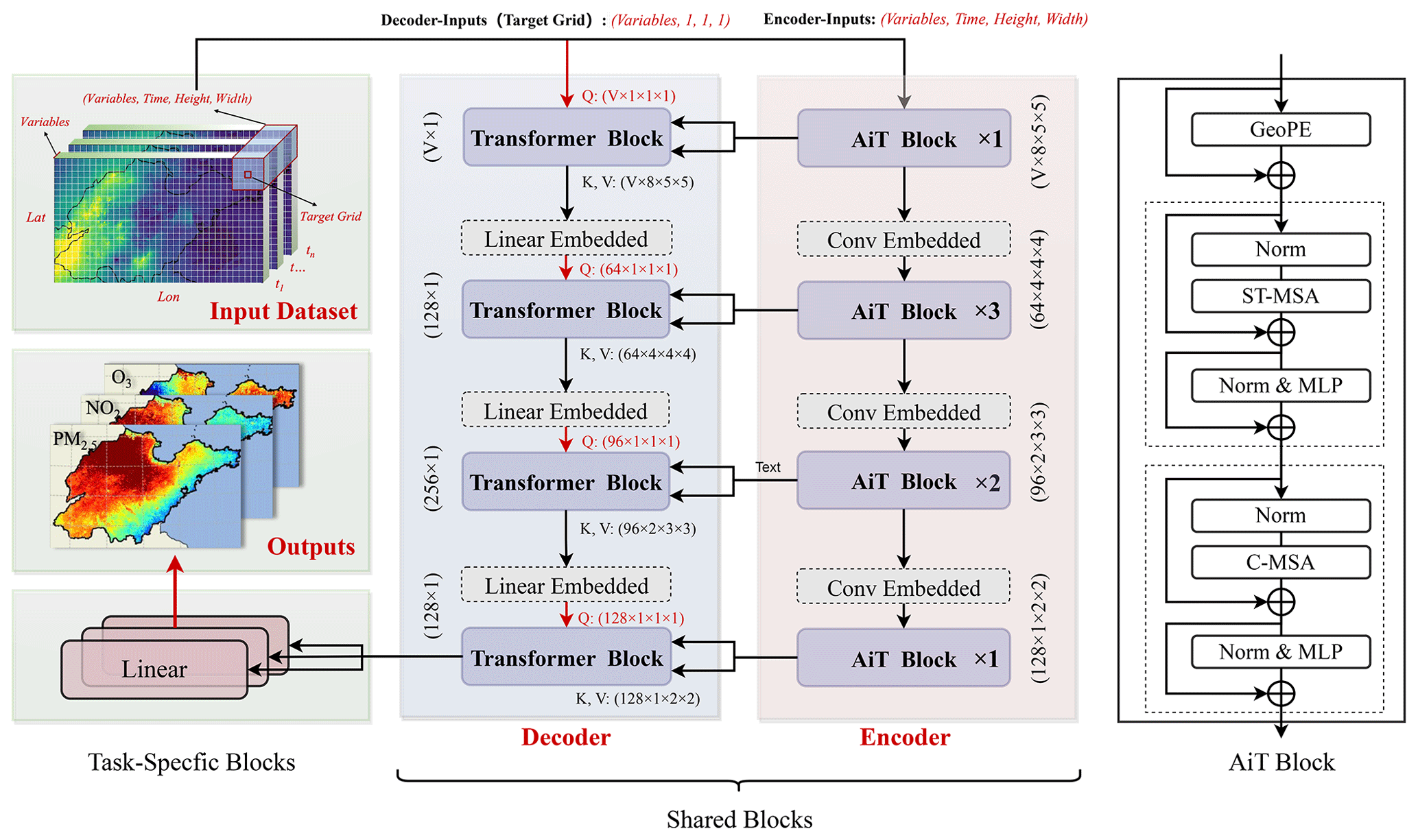
Figure 1 Schematic diagram of the AiT model. The white box of multi-dimension inputs presents each pixel of raster data. The AiT block is a transformer block based on self-attention across space, time, and variables. GeoPE, Norm, MLP, ST-MSA, and C-MSA respectively indicate positional embedding, layer normalization, multi-layer perceptron, spatial–temporal multi-head self-attention, and multi-channel (multi-variables) multi-head self-attention.

2.3 Diagnosing O₃ formation sensitivity

Interpretability can provide insight into how a model may be improved, bolster the understanding of the process being modeled, and engender appropriate confidence among researchers. SHAP is a coalitional game-theoretic approach based on Shapley values (Shapley, 1988) that assigns each variable an importance value for a particular estimation. Deep SHAP, a high-speed approximation algorithm that builds on the connection between Shapley values and DeepLIFT (Shrikumar et al., 2019), is employed to compute the feature importance of AiT from all data with monitoring labels for interpreting the prediction. The sensitivity of the O₃ formation regime was deduced using a combination of the XGBoost model and SHAP interpretability method, employing the GPUTreeShap algorithm (Mitchell et al., 2020), which simulated the response of surface O₃ to meteorological conditions, HCHO, NO₂, and PM_2.5, by utilizing the continuous estimations from ERA5, AiT, and TROPOMI between 2019 and 2020. The incorporation of meteorology in the model ameliorated the inadequacies in the conventional method (HCHO to NO₂ ratio), where its thresholds for identifying O₃ regimes vary temporally and spatially. The positive or negative contributions of three atmospheric pollutants were used to identify their promoting or inhibitory effects on O₃ variability. Given the unbiased property of SHAP values regarding directionality, the normalized relative magnitudes of SHAP values were calculated for HCHO, NO_2, and PM_2.5. This allowed the differentiation of the O₃ formation regimes based on the locally maximal proportions of the SHAP values for each species. The ground-level monthly HCHO concentrations were derived using a combination of the column-to-surface conversion factor (CF) simulated from the ECMWF Atmospheric Composition Reanalysis 4 and the tropospheric HCHO VCDs obtained from TROPOMI (Cooper et al., 2022; Su et al., 2022; Inness et al., 2019). A detailed description of the CF method as used here is discussed in Sect. S7. To ensure consistency in resolution between TROPOMI and AiT, we employed the oversampling method to downscale the TROPOMI VCDs to the resolution of AiT estimation, which has been proven effective in achieving finer resolution (Su et al., 2022; Cooper et al., 2022; van Donkelaar et al., 2015).

3 Results and discussion

3.1 Performance evaluation for the AiT

3.1.1 Cross-validation metrics

We evaluated the AiT performance using the 10-fold CV approach (Sect. S8), with the correlation coefficient (R²) measuring the extent to which model simulations explain variability in atmospheric pollutants and root mean square error (RMSE) and mean absolute error (MAE) evaluating the bias and error of the estimates. As shown in Fig. 2, out-of-sample CV daily ground-level O₃, NO₂, and PM_2.5 estimations are highly consistent with ground observations (R²=0.96, 0.92, 0.95), indicating low uncertainties, with RMSE of 10.1, 4.7, and 8.5 µg m⁻³ and MAE of 7.2, 3.5, and 5.3 µg m⁻³ for the 2018–2021 period. The linear regression comparing the O₃ predictions versus observations yields a slope of 0.98 and an intercept of 2.39, which demonstrates that there is no systematic bias in the estimations. Meanwhile, as shown in Fig. S3, our AiT model performs well at the individual site scale with high CV RMSE for O₃, NO₂, and PM_2.5 (10.5±8.6, 4.7±1.1, and 8.3±2.8 µg m⁻³). In general, the AiT model is robust for multi-pollutant simultaneous estimations.

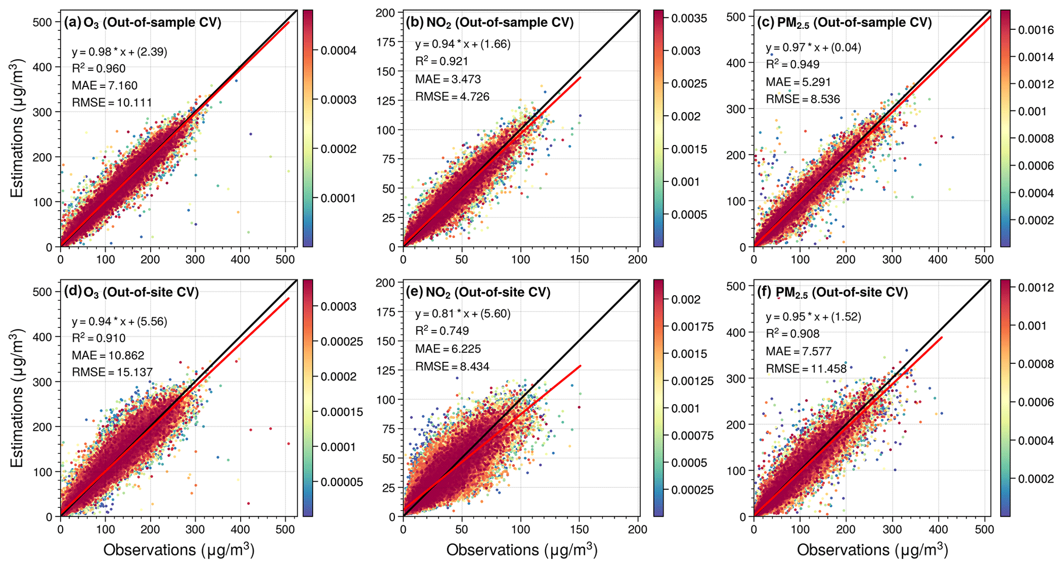
Figure 2 Out-of-sample cross-validation (a–c) and out-of-site cross-validation (d–f) of daily ground-level O₃, NO₂, and PM_2.5 concentration in the validation set.

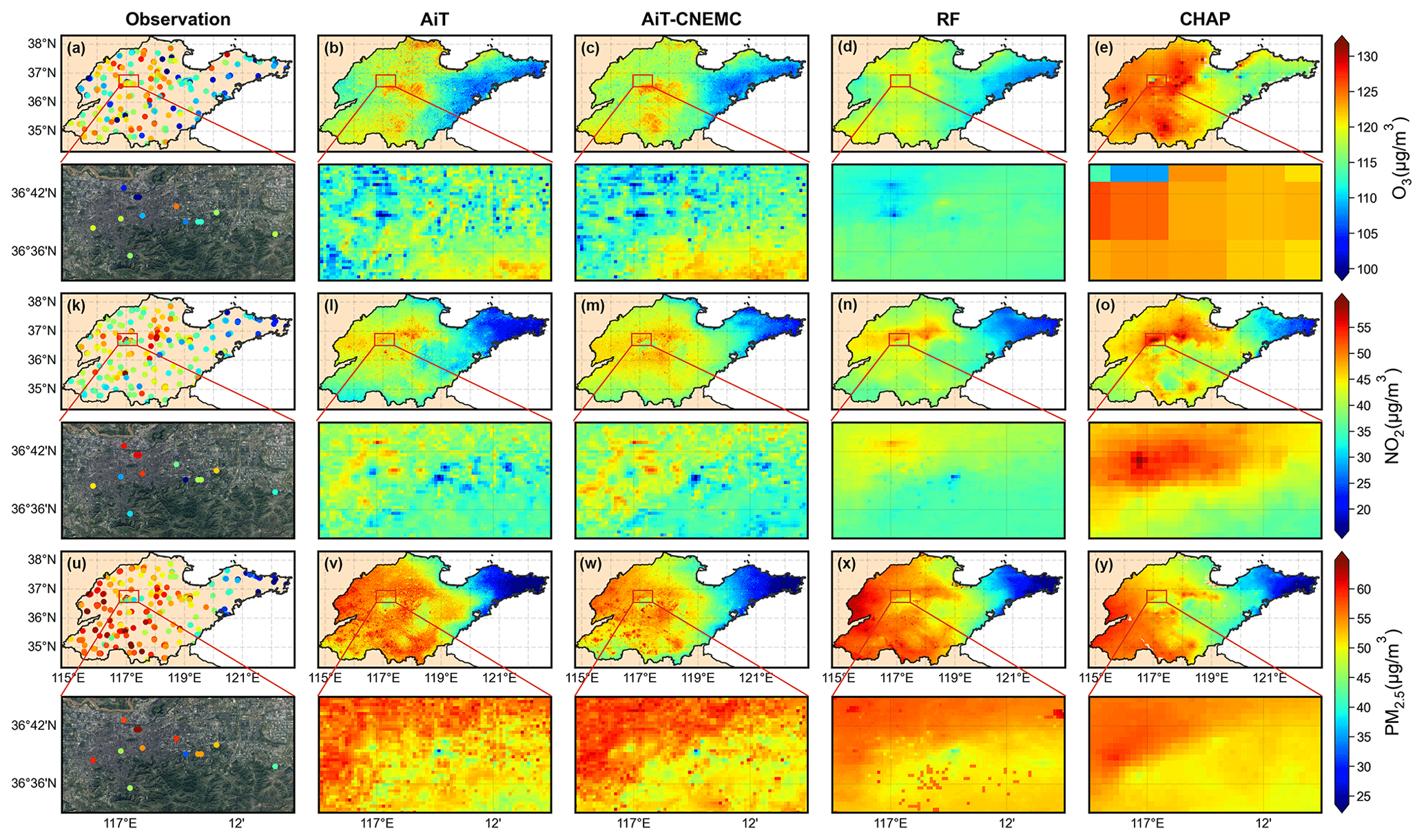
Figure 3 Spatial distribution of the annual mean (a–e) O₃, (k–o) NO₂, and (u–y) PM_2.5 concentrations from observations, Air Transformer (AiT), CNEMC-trained AiT, random forest (RF), and ChinaHighAirPollutants (CHAP), respectively, in 2019. The region enclosed by the red rectangular box corresponds to the zoomed-in maps of the satellite (©Tianditu: https://www.tianditu.gov.cn/, last access: 23 January 2024) and pollutant concentrations at a city scale for the capital city of Shandong province, Jinan.

The spatial generalization ability of the AiT is then examined by the out-of-site CV evaluation method (Fig. 2). The daily spatial variations of O₃, NO₂, and PM_2.5 at locations without ground measurements can be well estimated by our model (i.e., CV R²=0.91, 0.75, 0.91), representing a core contribution of such studies. We also probe the model performance for each site separately based on spatial CV estimations (Fig. S4). This general model yields an RMSE of 15.2±8.8, 8.1±2.7, and 11.1±2.8 µg m⁻³, respectively. Furthermore, we trained the AiT model using data exclusively from CNEMC and assessed its generalizability by validating it with data from SDEM. The model demonstrates strong performance with high our-of-sample CV R² values in the validation dataset of CNEMC (Fig. S5), and when evaluated with SDEM data, it exhibits only an acceptable degradation in predictive accuracy (Fig. S6, R² for O₃, NO₂, and PM_2.5: 0.90, 0.73, 0.79). Meanwhile, our framework utilizes multi-task learning to enhance computational efficiency through a single iteration and leverages the interactions among multiple pollutants to optimize the performance at individual pollutant levels (Table S2). In summary, AiT provides relatively stable estimations in areas without available ground-level monitoring and reliably extends ground monitoring from the site scale to the full-coverage spatial scale with high spatial resolution.

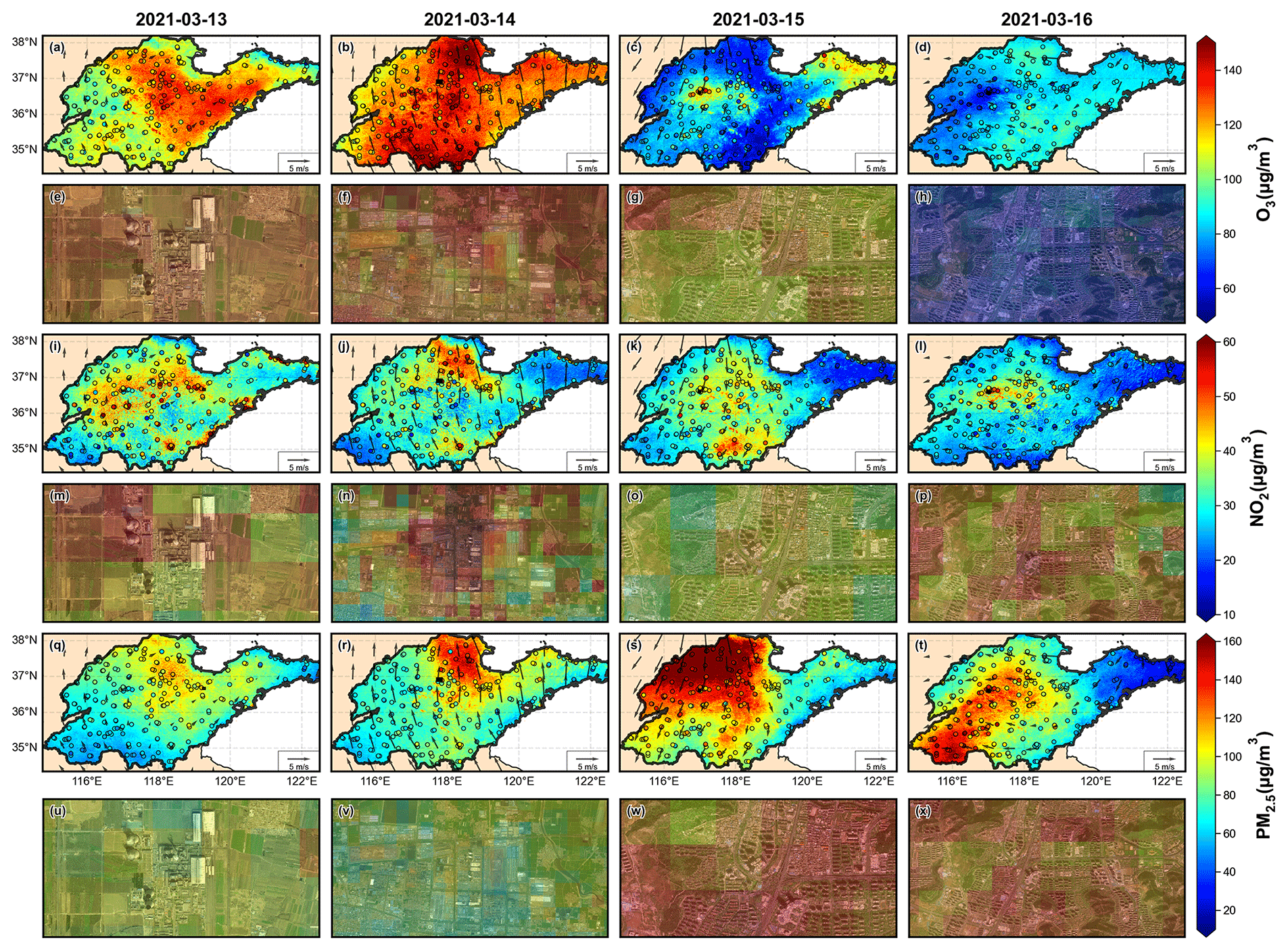
Figure 4 The spatial distribution of ground-level O₃ (a–d), NO₂ (i–l), and PM_2.5 (q–t) concentrations from AiT and monitoring stations during 13–16 March 2021 in Shandong, China. The black arrows are the 10 m wind speed and wind direction. The even-numbered rows correspond to the concentration distribution maps of typical emission sources for the respective pollutants, accompanied by satellite images (©Tianditu: https://www.tianditu.gov.cn/, last access: 23 January 2024). The upper right area of (e), (m), and (u) is a thermal power plant in Weifang (119°250^′–119°280^′E, 36°658^′–36°673^′N). The center area of (f), (n), and (v) is an industrial park in Zibo (117°725^′–117°845^′E, 36° 880^′–36°940^′N). The center and upper right area of (g), (o), and (w) represent an overpass and Wanling Mountain in Jinan (116°977^′–117°009^′E, 36°590^′–36°606^′N). The center area of (h), (p), and (x) is another overpass in Jinan (116°970^′–117°030^′E, 36°580^′–36°610^′N).

3.1.2 Compared with other ML models

Since ground-level air quality measurements across the target regions are extremely limited at a 500 m spatial resolution, representing only roughly 2 $/$ 1000 of the total grid cells, we seek implicit approaches to validate our estimated near-surface pollutant concentrations. We compared the model performance with previous studies that applied different ML methods to estimate these three air pollutants individually and found that our cross-validation results are comparable to or even better than those (Table S3). We also created a new dataset in our study by applying the classic RF algorithm, which is the most common ML model for estimating atmospheric pollution in recent years (Wei et al., 2022a; Requia et al., 2020; Xiao et al., 2018; Geng et al., 2021; Lu et al., 2021) with the same variables as AiT. The statistical comparisons between AiT and RF are also shown in Table S3. We then compared the spatial distribution of our results with estimations from CHAP, AiT-CNEMC, and RF.

Figure 3 shows the spatial maps of near-surface air pollutants with partially zoomed satellite images for monitoring sites, AiT, CNEMC-trained AiT, RF, and CHAP in 2019 (see Fig. S7 for 2020). We found that the estimated NO₂ and PM_2.5 from the AiT share a similar spatial distribution to those estimated by RF and CHAP. However, enlarged city-level urban regions in Fig. 3 reveal that AiT estimates fine structures and intra-urban disparities in near-surface multi-pollutant concentrations, which cannot be captured by either RF or CHAP products. This spatial gradient is also captured by AiT trained with CNEMC data, revealing the reliability of the deep learning model structure. In general, while RF and CHAP can only identify the hotspots of air pollutants at a regional scale, the spatial distribution of air pollutants estimated by AiT shows much more detailed differences with high spatial and temporal variability across the city scale. The differences of near-surface annual averaged pollutants between 2019 and 2020 for measured and multi-estimated data are presented in Fig. S8. The reductions or increases in O₃, NO₂, and PM_2.5 in distinct locations can be simulated by our model, which is relatively consistent with the changes in measurements. The zoomed maps in Fig. S8 show the differences in three pollutant concentrations at the city scale of the capital of Shandong province, Jinan. It can be found that the change in pollutant levels in 2020 compared to 2019 exhibits substantial regional variations and intra-urban heterogeneity, with some areas experiencing an increase and others a decrease. Compared to the estimations of RF and CHAP, our results successfully capture the complex distribution of air pollution in reality and reveal that the decline in PM_2.5 is primarily concentrated in suburban areas, while an increase is pronounced in some urban regions during 2020. Notably, this spatial trend may be consistent with underlying emission patterns and meteorological conditions.

3.1.3 Typical event study

The typical example of the spatial distribution of multi-pollutant observations and estimations of AiT is compared for validating the predictive capability of the model during a particular pollution episode, i.e., 13–16 March 2021. During this period, an early-season dust storm, which was called the largest and strongest such storm in a decade, hit northern China (Myers, 2021). As shown in Fig. 4, our model can capture the spatial distribution of surface O₃, NO₂, and PM_2.5 at the time of severe atmospheric pollution. In addition, our estimations are in high concordance with measurements in terms of magnitudes and spatial variability over the entire research region. The model trained solely on CNEMC data is also capable of effectively capturing the drastic changes in air quality during the pollution episode (Fig. S9). Combining wind fields to analyze PM_2.5 distribution on the day of the dust storm, it can be found that surface wind carries a massive amount of particulate matter from Beijing, which suffered a severe dust storm, to northern Shandong. The influence was gradually diminishing in southern Shandong due to the obstruction of Mount Tai. Spatial heterogeneity within intra-urban areas was further investigated to identify the hotspots of pollution sources. The satellite images in even-numbered rows of Fig. 4 illustrate the spatial disparities of three pollutants around four typical emission sources: thermal power plants, industrial parks, overpasses, and parks. As depicted, these anthropogenic emission sources contribute to higher pollution levels, while the mountain in the park mitigates primary pollution but also increases O₃ concentrations. Industrial sources emit a large amount of NO_x and PM_2.5, leading to increased pollution of these species compared with other urban microenvironments, which in turn promotes O₃ formation, particularly in downwind areas (Miller et al., 1978; Tang et al., 2020). Although the spatial gradients of pollutants on the street are not as apparent as in the dataset with 100 m resolution (Huang et al., 2021), the predicted spatial variation between various geographical scenes is in satisfactory agreement given the 500 m scale of the model. Urban areas affected by diverse dust pollution exhibit lower PM_2.5 concentrations compared to rural areas due to the obstructive and filtering effects of artificial structures, such as buildings and urban greenery (Fig. S10), which cannot be effectively captured solely by ground-based observations. Notably, the elevated PM_2.5 inhibits the formation of O₃ by diminishing solar radiation flux and absorbing the HO₂ radical on the aerosol surface, even in conditions characterized by similar NO₂ levels. As for the mapping, AiT accurately grasps the spatial characteristics of air pollutants and delivers a coherent spatial–temporal distribution that is consistent with the prior knowledge of atmospheric transport.

3.2 Urban–nonurban difference

Full-coverage pollutant estimates provide a foundational basis for assessing urban–nonurban disparities, addressing the critical issue of imbalanced site numbers between urban and rural locations. Table S4 shows the concentrations of O₃, NO₂, PM_2.5, and HCHO over the urban and nonurban regions, delineated from an annual urban extent dataset (Zhao et al., 2022). The urban extents in Shandong province in 2019 are depicted in Fig. S11. From 2019 to 2020, surface air pollutant levels declined significantly in Shandong. The averaged concentration discrepancies of these pollutants between urban and nonurban areas over February to March (lockdown during COVID-19) and June to October (summertime) are shown in Fig. 5. Surface concentrations of NO₂ and HCHO are higher in urban than nonurban areas, and the differences narrowed from February to October, while PM_2.5 is the opposite in both. Ground-level O₃ levels exhibited unexpected urban–nonurban disparity variations from the lockdown period through the summer as well as from 2019 to 2020. Compared to nonurban areas, the urban areas, which previously had lower O₃ levels, began to experience higher concentrations, attributed to a more rapid decline of ozone in nonurban regions. Figure 6 reveals that urban–nonurban differences in O₃ and PM_2.5 varied across various cities during the lockdown period in 2019, while the higher NO₂ pollution in urban areas remained consistent. In summer, only a handful of urban areas exhibit lower levels of ozone concentration, where NO₂ and PM_2.5 levels surpass those in nonurban regions, attributable to a more pronounced titration effect of NO and a slower rate of photochemistry reactions (Fig. S12) (Sicard et al., 2016, 2020; Zhang et al., 2004). Comparative urban–nonurban differences from 2019 to 2020 indicate an accelerated reduction of ozone and HCHO in nonurban areas, while NO₂ and PM_2.5 levels in urban areas saw a more significant decrease due to the decline in anthropogenic activities, particularly the suspension of emissions from pollution sources located in urban areas. Upon comparing the results of urban–nonurban disparities of our data with monitoring data and the CHAP dataset, we have identified potential overestimations or underestimations across various cities in monitoring data, likely resulting from the limited number of nonurban sites (Figs. 6m and S13). The notable disparity between the number of urban and nonurban sites in cities such as JNA, LC, LY, QD, and YT results in a pattern of urban–nonurban differences that contrasts markedly with that observed in AiT (Table S5). The urban–nonurban difference calculated by CHAP generally aligns with our findings (Fig. S14). Nevertheless, it is worth noting that the coarse resolution of O₃ (10 km) has led to a significant overestimation. These results highlight the value of high-resolution and gapless data for studying urban–nonurban disparities.

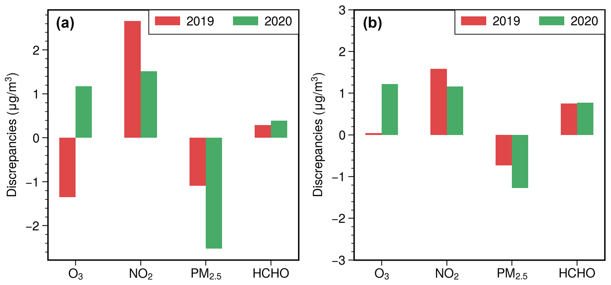
Figure 5 The discrepancies of O₃, NO₂, and PM_2.5 between urban and nonurban areas from 2019 to 2020 for the lockdown period (a) and the summertime (b) averaged concentration.

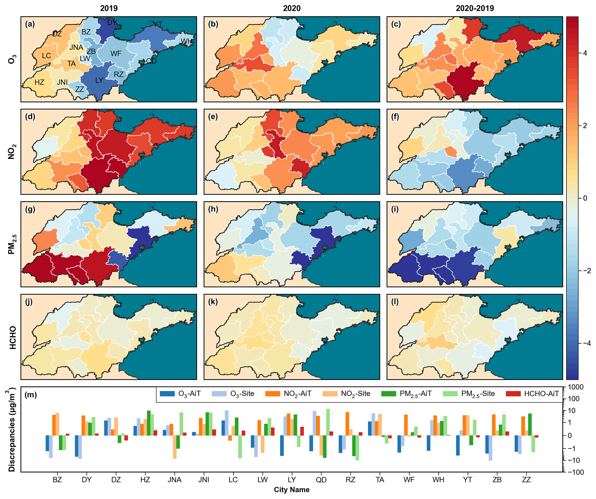
Figure 6 The urban–nonurban disparities of O₃, NO₂, PM_2.5, and HCHO calculated by AiT across cities with administrative divisions in Shandong, China, during lockdown periods in 2019 (a, d, g, j) and 2020 (b, e, h, k), as well as the changes in differences between 2019 and 2020 (c, f, i, l). Panel (m) is the comparison between the results of monitoring station data and the AiT dataset in 2019. Red represents a greater decline in air pollutants in nonurban areas, while blue indicates a more significant reduction in urban areas in the third column of the figure (YT: Yantai, BZ: Binzhou, DY: Dongying, WH: Weihai, DZ: Dezhou, JNA: Jinan, QD: Qingdao, WF: Weifang, ZB: Zibo, LC: Liaocheng, LW: Laiwu, TA: Taian, LY: Linyi, RZ: Rizhao, JNI: Jining, HZ: Hezhe, ZZ: Zaozhuang).

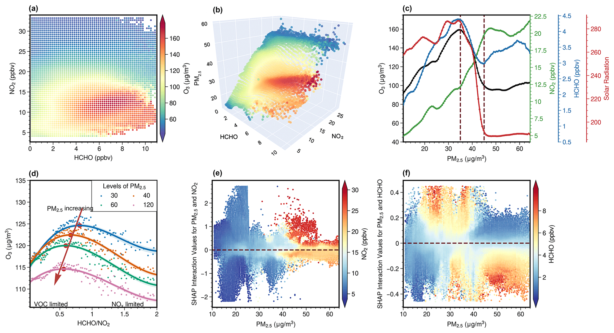
Figure 7 (a) O₃ concentrations as a function of surface HCHO and NO₂. (b) O₃ concentrations as a function of surface HCHO, NO₂, and PM_2.5. Both (a) and (b) utilize a shared color bar to indicate O₃ concentrations, enhancing comparability. (c) Relationship between O₃, and NO₂, HCHO, and surface shortwave radiation flux. The paired O₃, HCHO, NO₂, and solar radiation are divided into 100 bins based on PM_2.5, and then the averaged concentrations (y axis) are calculated for each PM_2.5 bin (x axis). (d) Changes in the $\mathrm{HCHO}/{\mathrm{NO}}_{\mathrm{2}}$–O₃ relationship in response to changing PM_2.5 by the XGBoost model. The solid lines are fitted with fourth-order polynomial curves, and the shading indicates 95 % confidence intervals. (e–f) The interaction between SHAP values reveal an interesting hidden relationship between pairwise variables (PM_2.5, NO₂, HCHO) and O₃.

3.3 Photochemical regimes

3.3.1 Ozone–NO_x–VOC–aerosol sensitivity

Figure S15 shows the seasonal maps of O₃, PM_2.5, and NO₂ estimations from AiT and satellite-derived surface HCHO. Based on these data, we first capture the well-established nonlinearities in O₃–VOC–NO_x chemistry with a conceptual framework similar to classic O₃ isopleths typically generated with models (Pusede et al., 2015; J. Ren et al., 2022). Figure 7a depicts O₃ concentration as a function of HCHO and NO₂, which was derived solely from ground-level estimation. The result indicates that the O₃ regimes can be qualitatively identified based on the nonlinear interaction between surface O₃, HCHO, and NO₂. In the regime characterized by high NO₂ and low HCHO, the elevated consumption of HO_x, predominantly driven by the OH + NO₂ termination reaction, results in the suppression of NO_x on O₃, indicating the prevalence of VOC-limited chemistry. Conversely, when HCHO levels are high and NO₂ levels are relatively low, O₃ increases with NO₂ and exhibits insensitivity to HCHO due to abundant peroxyl radical (HO₂+ organic peroxy (RO₂) radicals, RO_x) self-reactions, suggesting NO_x-limited (VOC-saturated) chemistry. In cases where high HCHO and NO₂, the O₃ increases with both HCHO and NO₂, reaching a peak. While Fig. 7a resembles this overall O₃–VOC–NO_x relationship, the blurry transition between two different regimes and the role of PM_2.5 are uncertain, which may be influenced by meteorological conditions, chemical and depositional loss of O₃, errors of estimations, and aerosol-inhibited regimes. Increasing PM_2.5 levels could suppress O₃ formation even under high HCHO and NO₂ conditions (Fig. 7b), which could be induced by enhanced reactive uptake of HO₂ onto aerosol particles and weaker photochemical reaction resulting from the scattering and absorption of solar radiation by anthropogenic aerosols. The relationship between PM_2.5 and O₃ in Shandong demonstrates the distinct stages of O₃ chemistry, as depicted in Fig. 7c. When PM_2.5 was below the maximum turning point (MTP1, 35 µg m⁻³), a linear and positive correlation between O₃ and PM_2.5 was observed due to the common dependence on precursors in the initial stage (Zhang et al., 2022). As PM_2.5 increased beyond the MTP1, a sharp reduction in HCHO and O₃ was observed, accompanied by a decline in surface shortwave radiation, reflecting their formation as photo-oxidation products of OVOCs and NO_x. When PM_2.5 exceeded the minimum transition point (MTP2, 45 µg m⁻³), a phase was observed with stagnant radiation intensity and relatively higher NO₂ levels compared to HCHO. This is typically associated with a VOC-limited regime, where an increase in HCHO and a decrease in NO₂ concentration could promote O₃ production. However, our findings demonstrated an opposite impact of HCHO and NO₂ on O₃ when PM_2.5 exceeded MTP2. Figure 7d shows the changes in the quantitative relationships between $\mathrm{HCHO}/{\mathrm{NO}}_{\mathrm{2}}$ (FNR) and O₃ by artificially changing PM_2.5 and precursor levels for XGBoost, in which the peak of curves marks the transitional threshold of O₃ regimes from VOC- to NO_x-sensitive. It can be seen that attenuated PM_2.5 pollution could increase the sensitivity of O₃ to VOCs and decrease the sensitivity to NO_x, which causes the shift in O₃ regimes from NO_x-limited to VOC-limited. With the recent reduction in NO_x emissions in China, the anticipated transition of the O₃ production regime in urban areas towards being more NO_x-limited has been impeded by the heightened VOC sensitivity resulting from decreased PM_2.5 levels. Our results are consistent with the findings of Li et al. regarding the O_x–NO_x relationship in response to changing PM_2.5 (C. Li et al., 2022) and with the findings of Dyson et al. (2023) on the impact of HO₂ aerosol uptake on O₃ production (Dyson et al., 2023). The SHAP interaction plots in Fig. 7e and f illustrate that the influence of NO₂ and HCHO on O₃ formation is not constant and is influenced by the levels of PM_2.5. Typically, at a certain level of PM_2.5, a lower NO concentration results in a stronger inhibitory effect on O₃ production. This could be due to aerosols exerting stronger suppression through the HO₂ sink at lower NO_x levels. As the concentration of PM_2.5 increases, often accompanied by a concurrent increase in NO₂ as a key precursor, there is a greater need for higher levels of NO₂ to be converted into nitrous acid (HONO) through the heterogeneous uptake by aerosols. This process produces more OH radicals, which facilitate photochemical O₃ formation, thereby offsetting the increased inhibitory effect of the HO₂ sink. Under high PM_2.5 concentrations, an increase in NO₂ along with a decrease in HCHO enhances their effect on promoting O₃ formation. Meanwhile, the impact of HCHO shifts from promoting to suppressing as PM_2.5 pollution intensifies. It further illustrates that the scavenging of HO₂ on aerosols can cause the shift in O₃ regimes from being VOC-limited to NO_x-limited and the threshold approach is restricted by aerosols and meteorology for determining the constantly changing O₃ formation regimes over time and space.

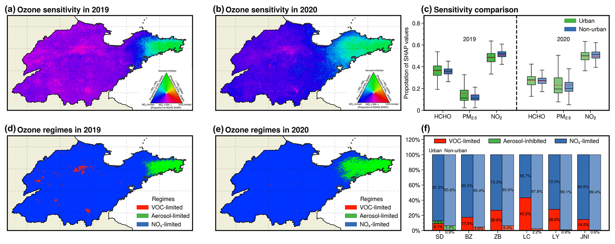
Figure 8 Comparison of geographical distribution for ozone formation regimes between 2019 and 2020 in the summertime. All surface daily O₃, PM_2.5, and NO₂ estimations from Air Transformer (AiT) are averaged over each month from May to October 2019–2020 for matching monthly HCHO derived from TROPOMI (500 ⋅ 500 m). (a, b) Geographical distribution of the fractional contribution of chemical factors representing O₃ formation regimes. The ternary phase diagram in the legend depicts the normalized fraction of SHAP values for O₃ attributed to HCHO, NO₂, and PM_2.5 at the surface, representing VOC-limited (red), aerosol-inhibited (green), and NO_x-limited (blue) regimes, respectively. (c) Statistical changes in the fractional contribution of chemical factors. (d, e) Geographical distribution of O₃ chemical regimes. (f) Proportion of three O₃ chemical regimes across urban and nonurban areas in 2019 in Shandong (SD) and individual cities (BZ: Binzhou, ZB: Zibo, LC: Liaocheng, LY: Linyi, JNI: Jining).

Unraveling the intricate interplay of O₃ with meteorology, aerosols, and precursors that govern O₃ formation over extensive spatial domains has long confounded robust interpretation. These multiscale processes were elucidated using an interpretable ML model, which can quantify the positive or negative contributions of individual processes. As depicted in Fig. S16, the performance of the XGBoost model is robust, evidenced by a high R² value of 0.99 coupled with a low RMSE of 3.24 µg m⁻³ and MAE of 2.33 µg m⁻³. Figure S17 shows that meteorological variations, chiefly surface shortwave radiation flux modulating photochemical reaction kinetics, primarily dictate the heterogeneous geographic distribution of O₃ at the regional scale, with lower levels over the Jiaodong Peninsula. Meanwhile, local atmospheric chemical processes predominate the city-scale variability of O₃. HCHO facilitated O₃ formation in urban areas yet suppressed it in rural regions across areas with high ozone, where most NO₂ promoted O₃ production overall, indicating VOC–NO_x synergistic control on O₃ in cities and a NO_x-limited regime in rural areas during summertime. The contribution of NO₂ and PM_2.5 exhibits analogous seasonal variability, promoting O₃ formation under low pollution conditions while inhibiting O₃ when pollution levels are high (Figs. S15 and 18). The elevated NO₂ levels in autumn led to a negative contribution to O₃, whereas the facilitating effect of PM_2.5 was enhanced. This stems from the relatively moderate PM_2.5 concentrations slightly affecting photochemical reaction rates, while the increased NO₂ amplified the reactive uptake of NO₂ by PM_2.5, generating more OH radicals that promote O₃ formation (Lin et al., 2023; Tan et al., 2022). In winter, PM_2.5 pollution exceeding 75 µg m⁻³ suppressed O₃ formation through scattering and absorbing solar radiation that activates atmospheric chemical processes, which counteracted the promoting effect of high PM_2.5 through the conversion of NO₂ to HONO.

Figure 8a–c show surface distribution and changes in the relative proportions of SHAP values on three pollutants for inferring O₃ photochemical regimes. Moving along an urban-to-rural gradient, reactions dominated by RO_x radical self-reactions are continuously enhanced with increasing NO_x SHAP values, resulting in the majority of rural Shandong being situated in NO_x-limited regimes. Furthermore, the overall ozone production regimes in Shandong exhibited a transition toward more NO_x-limited from 2019 to 2020, with regions dominated by NO_x-limited shifting toward being aerosol-inhibited in the Jiaodong Peninsula. The aerosol-inhibited regime differs from the two classically applied tropospheric O₃ policy-control regimes. It is attributed to the predominant heterogeneous HO₂ uptake by aqueous aerosols, despite comparatively low PM_2.5 levels during summertime. The marine environment produces liquid aerosol particles with HO₂ uptake coefficients exceeding those of dry aerosols by orders of magnitude (H. Song et al., 2022). Concurrently, lower ambient NO_x levels minimize the promotive effects of aerosols on ozone formation (Tan et al., 2022; Kohno et al., 2022). This result is consistent with the findings of Dyson et al. (Dyson et al., 2023), which concluded that the contribution of HO₂ sinks onto aerosols on total HO₂ could increase for areas with low NO levels. The attenuated responsiveness of O₃ formation to VOCs induced by the uptake of HO₂ results in enhanced sensitivity of NO_x at the northwestern boundary region of the Jiaodong Peninsula. Collectively, these processes delineate an aerosol-inhibited ozone production regime in this coastal region, reflecting the sensitivity of O₃ photochemistry to the HO₂ sink. In several cities, including Binzhou, Zibo, Liaocheng, Linyi, and Jining, a greater proportion of urban areas compared to their nonurban counterparts exhibited a VOC-limited regime in 2019, as indicated by the prevalence of red regions in Fig. 8d. The percentage of urban areas in these cities under a VOC-limited regime ranges from 15 % to 43 %, in stark contrast to nonurban areas where such a regime is typically rare (Fig. 8f). The comparison of O₃ sensitivities from 2019 to 2020 shows a regional shift towards increased sensitivity to aerosol and NO_x, along with a decreased VOC sensitivity as a result of NO_x reduction (Fig. 8a–c). This shift led to the majority of areas in Shandong being dominated by a NO_x-limited regime in 2020, with an expanded aerosol-inhibited regime region in the Jiaodong Peninsula (Fig. 8e). Additionally, the discrepancy in O₃ formation sensitivity between urban and nonurban areas was diminished during this period (Fig. 8c). As illustrated in Fig. 9, while the ozone regime transitions towards NO_x-limited, there is a marked shift towards greater aerosol sensitivity across nearly 90 % of areas, leading to a 1.6 % increase in aerosol-inhibited grids. Compared to nonurban regions, a higher number of grids in urban areas demonstrate a shift towards NO_x sensitivity. Conversely, urban areas that were predominantly aerosol-inhibited in 2019 showed a lower-sensitivity shift towards NO_x.

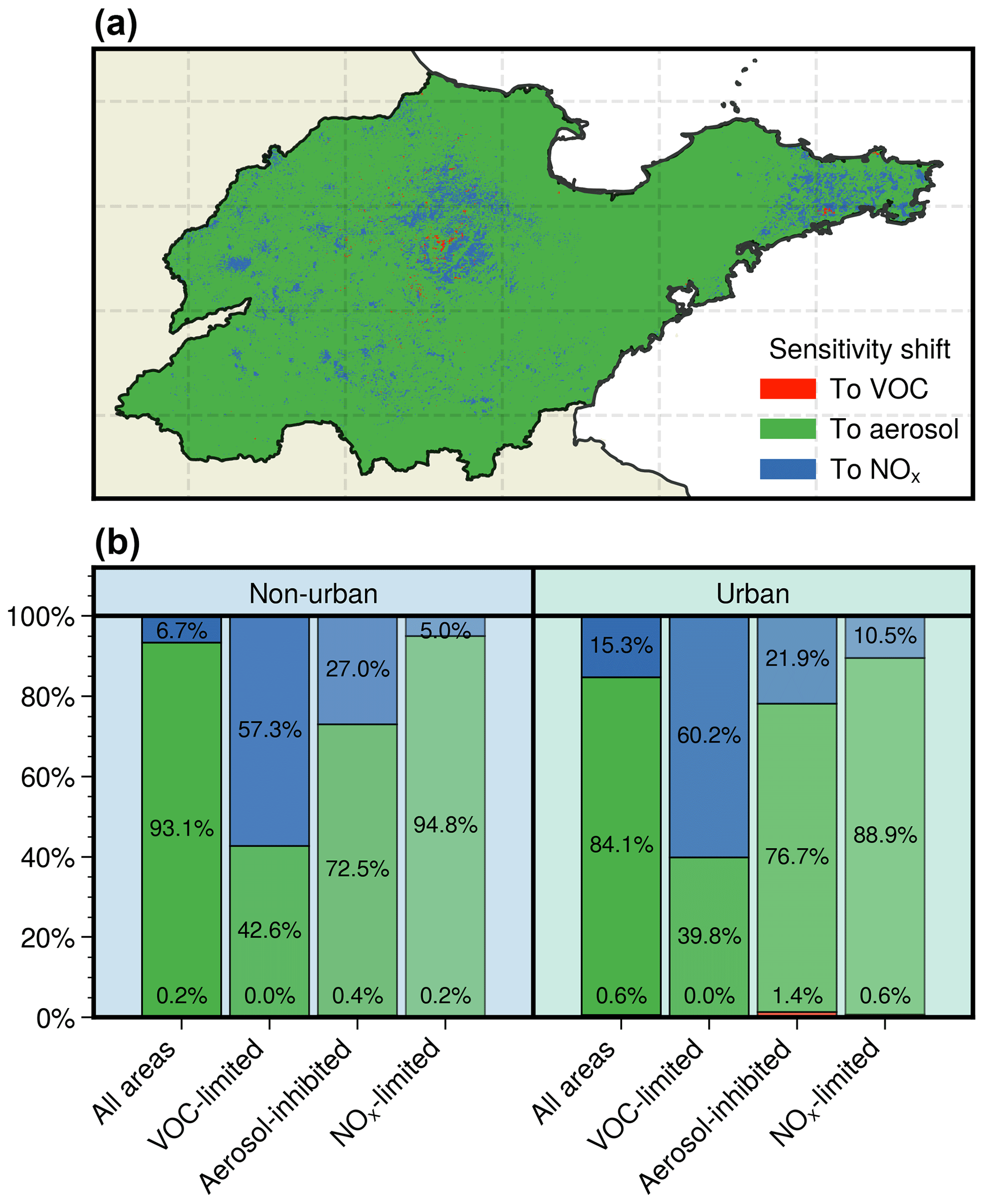
Figure 9 Geographical distribution of changes in ozone sensitivity from 2019 to 2020 in summertime (a). Comparison of ozone sensitivity changes across areas dominated by different chemical regimes in 2019 between urban and nonurban areas (b).

3.3.2 Impact on urban–nonurban differences

We further explore the reversed O₃ differences by separating the individual contributions of climate and anthropogenic changes using an interpretable machine learning model (Fig. 10). The results demonstrate that atmospheric chemical processes and meteorological conditions commonly dominate the discrepancies in O₃ levels between urban and nonurban areas. From 2019 to 2020, meteorological shifts remained uniform across urban and nonurban regions, marked by lowered surface pressure, boundary layer height, and shortwave radiation, alongside heightened precipitation. This, coupled with decreased precursor levels, contributed to a decline in O₃ pollution. As shown in Figs. 10 and S19, the diminished reduction in boundary layer height and radiation flux across urban areas, compared to nonurban areas in 2020, decelerated the expected decline of O₃ concentrations, leading to urban O₃ levels exceeding those of nonurban areas. Concurrently, a narrowing difference in temperatures between urban and nonurban areas, despite an overall cooling from 2019 to 2020, favored O₃ formation in urban regions during the summertime. Additionally, PM_2.5 emerged as the principal anthropogenic factor inverting the urban–nonurban O₃ disparity over the course of 2019 to 2020. Its contribution to ozone shifted from being lower in urban areas to exceeding that in nonurban areas, revealing that the decreased reactive uptake of HO₂ from aerosols induced by a more substantial reduction in PM_2.5 in urban areas made the larger contribution to O₃ production (Ivatt et al., 2022; Li et al., 2017). Moreover, the response of O₃ to the changes in its precursors and PM_2.5 was determined by the O₃ formation regimes. The variations in O₃ sensitivity also corroborate the above finding. In rural areas, where there was less of a reduction in PM_2.5 concentration, the sensitivity increasingly favored aerosol suppression across more than 93 % of the assessed grids (Fig. 9). This enhanced suppression effect of aerosols in rural areas leads to a more significant O₃ reduction compared to urban locales. The reduction of NO_x in nonurban areas demonstrated a more effective reduction in O₃ levels, which predominantly shifted towards a NO_x-limited regime in 2020. Although urban areas also showed a shift towards being a NO_x-limited regime, they exhibited relatively higher sensitivity to VOCs (Fig. 8). The urban areas, characterized by elevated NO_x emissions, exhibited a higher sensitivity to VOCs, and the fraction of aerosol-inhibited areas increased from 2019 to 2020, resulting in the control benefits of urban O₃ pollution in 2020 being partially offset by the nonlinear response of O₃ to a greater reduction in NO₂ and PM_2.5, as well as a smaller decrease in HCHO relative to nonurban areas. Consequently, O₃ exhibits a lower reduction in urban areas as a result of the aforementioned changes.

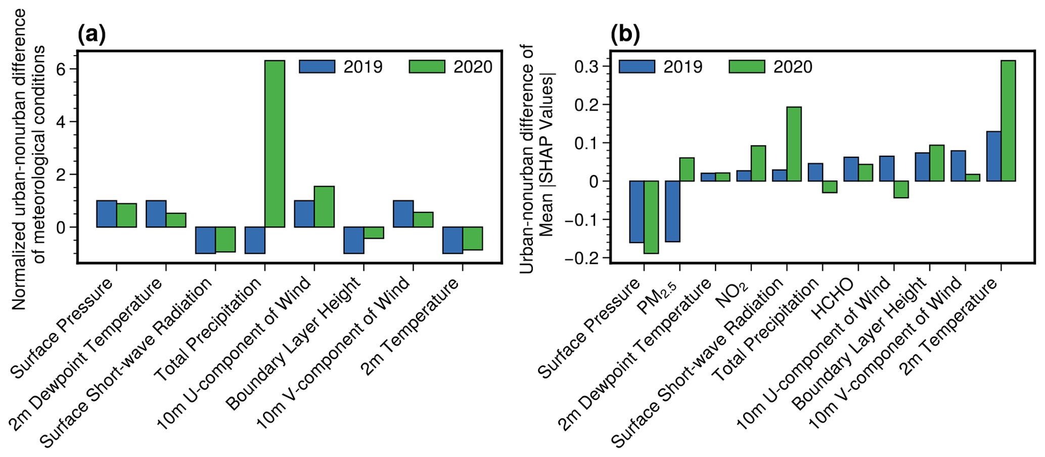
Figure 10 Comparison of urban–nonurban disparities in meteorological conditions (a) and mean absolute SHAP values (b) between 2019 and 2020 across Shandong, China, during the summertime.

4 Conclusions

The purpose of the current study was to diagnose the nonlinearity of O₃–NO_x–VOC–aerosol chemistry using an interpretable ML model based on spatially resolved multi-pollutant estimations for determining the causes of changing differences in O₃ levels between urban and nonurban areas. Our study represents the first attempt to develop an advanced DL model that reconstructs the concentrations of multiple pollutants and subsequently infers the aerosol-inhibited regime from observations. This innovative approach provides further support for investigating the impact of precursor emissions and aerosol on the urban–nonurban differences in O₃ levels.

Given the nonlinearity of ozone formation and its increasing regional differences, precise estimations of ground-level O₃, NO₂, HCHO, and PM_2.5 are crucial for deducing the chemical regimes governing ozone pollution and its urban–nonurban disparities. The evaluation of the model's performance indicates that it can be readily extended to any other domain thanks to its unified architecture. Anyone can easily utilize the model to estimate ground-level pollutants, intelligently considering spatial–temporal neighborhood information based on their customized input data. The model further improved spatial resolution to sub-kilometer levels using TROPOMI and MODIS retrievals via spatiotemporal autocorrelation downscaling of AiT. The “black box” nature of AiT can be made more physically interpretable by SHAP, enabling the evaluation of the significance of each input variable (Fig. S20). The season trends show the highest contribution, followed by emission proxies and meteorological conditions. Meanwhile, the results between AiT trained with all data and that trained exclusively with CNEMC data across various spatiotemporal scales underscore the promising prospect for improving the model's generalization ability with more ground-level monitoring data and the growing space of methods.

We conclude that with the effective reduction of PM_2.5 pollution, the sensitivity of O₃ to VOCs will increase, necessitating further intensification of VOC emission regulation by government agencies. Three distinct chemical regimes were assessed by tracking NO_x, VOCs, and aerosols with surface NO₂, HCHO, and PM_2.5. In the Jiaodong Peninsula of Shandong province, coastal areas with relatively few primary pollutants are widely found to be under an aerosol suppression regime, illustrating that ozone regime inference based on machine learning can serve as an alternative to determining the aerosol suppression regime through the rate of radical termination in atmospheric chemical models. The O₃ regime in other areas of Shandong generally transitioned from the NO_x-sensitive regime in nonurban to a more VOC-sensitive regime in urban areas. We estimate that substantial reductions in anthropogenic emissions of PM_2.5 and NO₂ are the main drivers of the reversal of the traditional discrepancy in O₃ levels between urban and nonurban areas. In essence, due to the lower efforts in reducing PM_2.5 in nonurban settings, the aerosol-mediated suppression of ozone became more pronounced, resulting in lower ozone levels in rural areas relative to urban centers. This shift underlines the intricate balance between emission reduction and ozone formation mechanisms, suggesting that nuanced understanding and targeted interventions are necessary to manage and mitigate the health and environmental impacts of such disparities. To preclude exacerbated O₃ pollution resulting from the shift of many regions from VOC-limited to NO_x-limited regimes and the decline in heterogeneous HO₂ uptake induced by PM_2.5 reduction in urban areas, emission policies aimed at decreasing NO_x to reduce O₃ levels will only be effective with stringent VOC emission abatement when PM_2.5 is concurrently decreased. The integration of high-resolution pollutant estimations with an interpretable machine learning model offers a promising avenue for advancing our understanding of ozone pollution dynamics and developing effective air quality management strategies.

Although our study endeavors to establish O₃ formation regimes involving NO_x, VOCs, and aerosols, and the method identifies an aerosol-inhibited regime from a statistical perspective, it is subject to certain uncertainties due to the relatively poor data quality of HCHO and the unsegregated multiple impacts of aerosols, such as N₂O₅ uptake, NO₂ uptake, HO₂ uptake, and light extinction (Tan et al., 2022). We have made efforts to integrate all required surface pollutant concentrations into a unified model, while the absence of ground-level HCHO monitoring data compelled us to tap into an alternative methodology. The retrieval error of surface HCHO and the system error between its retrieval approach and the AiT model degrade the ability of ML to identify the O₃ sensitivity. Meanwhile, the notion of ozone regimes is only appreciated in photochemically active environments where the RO_x–HO_x cycle is active (Souri et al., 2023). The definition of NO_x-limited or VOC-limited regimes is meaningless in nighttime chemistry, where NO–O₃–NO₂ partitioning is the primary driver. The surface daytime pollutant estimations with finer resolutions in space and time based on a unified modeling framework will offer an unprecedented view to characterize the near-surface O₃ formation regimes. Notwithstanding the relatively limited duration of the study, this work offers valuable insights into the current state and causes of urban–nonurban disparities in O₃ pollution. Future efforts should conduct a more detailed long-term evaluation of urban–nonurban disparities in global O₃ levels and the impact of formation mechanisms to further our understanding of air pollution and its mitigation.