the Creative Commons Attribution 4.0 License.
the Creative Commons Attribution 4.0 License.
 | 22 Feb 2024
Contrail formation on ambient aerosol particles for aircraft with hydrogen combustion: a box model trajectory study
Andreas Bier
Simon Unterstrasser
Josef Zink
Dennis Hillenbrand
Tina Jurkat-Witschas
Annemarie Lottermoser
Future air traffic using (green) hydrogen (H2) promises zero carbon emissions, but the effects of contrails from this new technology have hardly been investigated. We study contrail formation behind aircraft with H2 combustion by means of the particle-based Lagrangian Cloud Module (LCM) box model. Assuming the absence of soot and ultrafine volatile particle formation, contrail ice crystals form solely on atmospheric background particles mixed into the plume. While a recent study extended the original LCM with regard to the contrail formation on soot particles, we further advance the LCM to cover the contrail formation on ambient particles. For each simulation, we perform an ensemble of box model runs using the dilution along 1000 different plume trajectories.
The formation threshold temperature of H2 contrails is around 10 K higher than for conventional contrails (which form behind aircraft with kerosene combustion). Then, contrail formation becomes primarily limited by the homogeneous freezing temperature of the water droplets such that contrails can form at temperatures down to around 234 K.
The number of ice crystals formed varies strongly with ambient temperature even far away from the contrail formation threshold. The contrail ice crystal number clearly increases with ambient aerosol number concentration and decreases significantly for ambient particles with mean dry radii ⪅ 10 nm due to the Kelvin effect.
Besides simulations with one aerosol particle ensemble, we analyze contrail formation scenarios with two co-existing aerosol particle ensembles with different mean dry sizes or hygroscopicity parameters. We compare them to scenarios with a single ensemble that is the average of the two aerosol ensembles. We find that the total ice crystal number can differ significantly between the two cases, in particular if nucleation-mode particles are involved.
Due to the absence of soot particle emissions, the ice crystal number in H2 contrails is typically reduced by more than 80 %–90 % compared to conventional contrails. The contrail optical thickness is significantly reduced, and H2 contrails either become visible later than kerosene contrails or are not visible at all for low ambient particle number concentrations. On the other hand, H2 contrails can form at lower flight altitudes where conventional contrails would not form.
- Article
(4341 KB) - Full-text XML
- BibTeX
- EndNote


The contribution of aviation to the total anthropogenic climate forcing is estimated to be around 3.5 % (Lee et al., 2021). Besides the aircraft CO2 emissions, contrail cirrus makes a large contribution to the aviation radiative forcing (e.g., Boucher et al., 2013; Bock and Burkhardt, 2016b; Bier and Burkhardt, 2022). There are several measures to mitigate the climate impact due to contrail cirrus. One mitigation option is reducing the number of formed contrail ice crystals, which strongly impact the further contrail cirrus life cycle and the radiative forcing (e.g., Unterstrasser and Gierens, 2010; Bier et al., 2017; Burkhardt et al., 2018). This might be achieved by reducing soot particle number emissions, since contrail ice crystals form in particular on soot particles relative to co-emitted organic-sulfate particles for conventional passenger aircraft engines (e.g., Kärcher and Yu, 2009; Kleine et al., 2018). Several ground and flight measurement campaigns have shown significant reductions in engine soot number emissions using alternative fuel blends with a lower aromatic content (e.g., Moore et al., 2017; Voigt et al., 2021; Bräuer et al., 2021). Switching from the reference Jet A-1 fuel to semisynthetic or biofuel blends, Voigt et al. (2021) and Bräuer et al. (2021) also find significant reductions in young-contrail ice crystal numbers by around 20 %–70 %. Burkhardt et al. (2018) and Bier and Burkhardt (2022) emphasize that there is a strong non-linearity between the global contrail cirrus radiative forcing and the young-contrail ice crystal number. Hence, even larger reductions in the number of ice crystals formed are desirable to obtain a substantial mitigation effect.
Combustion of (green) hydrogen (H2) is a promising technology to reduce the overall aviation climate impact. It provides around 3 times more energy per fuel mass than kerosene fuel (Najjar, 2013), but it delivers much less energy by volume in typical atmospheric conditions. Hence, H2 is typically brought to liquid phase at 20 K and stored in special tanks of the cryoplane. During H2 combustion, the main emission product is water vapor and its emission is roughly a factor of 2.6 larger compared to kerosene for the same amount of released combustion energy and a similar propulsion efficiency (e.g., Schumann, 1996). Increased water vapor emissions in the stratosphere would cause significant radiative warming (Pletzer et al., 2022), but this impact would be low as long as the aircraft fly at altitudes in the troposphere (e.g., Wilcox et al., 2012). While NOx is still produced due to high flame temperatures, we expect neither direct CO2 nor soot particle emissions during H2 combustion. However, it was observed in laboratory studies that the emission of lubricant oil vapors can lead to the formation of ultrafine volatile particles (Ungeheuer et al., 2022). In ground field measurements, lubrication oil droplets with volumetric mean dry radii ranging between around 125–175 nm were observed by sampling directly from the breather vents (Yu et al., 2010). Furthermore, Yu et al. (2012) performed the first field study that investigates in-flight lubrication oil emissions behind a commercial aircraft. Thereby, they find a significant contribution of lubrication oil constituents in organic particulate matter emissions from the engine exhausts that are typically associated with high soot number emissions.
At the moment, measurements on H2 contrails do not exist. Airbus and the Deutsches Zentrum für Luft- und Raumfahrt (DLR) are planning measurements behind a glider equipped with a small H2 combustion engine within the Blue Condor campaign (Airbus, 2022). Moreover, Airbus aims at establishing the world's first commercial aircraft based on hydrogen propulsion by 2035 within the ZEROe project. Marquart et al. (2005) and Ponater et al. (2006) estimated the radiative forcing (RF) of line-shaped contrails for a hypothetical fleet of cryoplanes in comparison with a conventional fleet within a global climate model (GCM). They found similar RF values for both types of fleets. The decrease in optical thickness for H2 contrails (RF down) was roughly balanced by the larger contrail coverage (RF up). This estimate is based on a simple parameterization of line-shaped contrails (Ponater et al., 2002), where, e.g., the contrail cover scales with the contrail formation frequency and the ice water content is simply diagnosed by the atmospheric water vapor available for deposition. Recent GCM contrail parameterizations are more advanced as they simulate the full contrail (cirrus) life cycle; treat contrails as a separate cloud class to natural clouds; and introduce contrail ice water content, coverage and ice crystal number as prognostic variables (Bock and Burkhardt, 2016a; Bier and Burkhardt, 2022).
The hot exhaust plume behind the aircraft engines continuously expands and cools due to entrainment of ambient air. Under certain atmospheric conditions and depending on specific engine and fuel parameters, the plume humidity temporally surpasses water saturation in the early jet phase and enables the formation of contrails. This condition is described by the Schmidt–Appleman (SA) criterion (Schumann, 1996), which is based purely on the thermodynamics of the plume mixing process. If the SA criterion is fulfilled, plume particles can activate into water droplets (e.g., Kärcher and Yu, 2009; Kärcher et al., 2015). They subsequently turn into ice crystals by homogeneous freezing if ambient temperature is below the homogeneous freezing temperature. Switching to H2 combustion with expected soot-free emissions, contrail ice crystals can still form on upper-tropospheric (UT) background particles that are entrained into the plume (e.g., Kärcher et al., 1996, 2015).
Some recent box model studies and analytical approaches (Kärcher and Yu, 2009; Kärcher et al., 2015; Bier and Burkhardt, 2019) have already included ice crystal formation on ambient particles mixed into the plume. They show that this process will become relevant if soot number emissions from conventional aircraft engines are reduced by at least 2 orders of magnitude (referred to as “soot-poor emissions”). Kärcher (2018) estimate a decrease in the contrail ice crystal number by around 1–2 orders of magnitude when switching from conventional to soot-poor emissions at ambient temperatures at which ice crystals cannot form on ultrafine volatile particles. While those studies in general assumed fixed ambient particle properties, Lewellen (2020) investigated contrail formation on ambient aerosol (besides soot and volatile particles) in a box model and large-eddy simulation (LES) model and varied the ambient aerosol number concentration. Finally, we expect a high uncertainty in the estimated H2 contrail ice crystal number due to a large variability in atmospheric particle properties (e.g., Minikin et al., 2003; Hermann et al., 2003; Brock et al., 2021; Voigt et al., 2022), which has not been examined in sufficient detail before. Moreover, it is not clear whether ultrafine volatile particles originating from lubrication oils and NOx emissions play a role in droplet and ice crystal formation.
The contrail formation studies mentioned in the preceding paragraph have been performed only for fuel and engine parameters that represent the kerosene case and consider the competition between ambient aerosol, soot and volatile particles. Ström and Gierens (2002) is the only contrail evolution study considering aircraft with H2 combustion. They performed 2D simulations of young contrails including the contrail formation process in the jet phase. They prescribe a bi-modal log-normal aerosol size distribution and vary the aerosol number concentration as the most relevant input parameter. They employ a bulk approach for the treatment of the ice microphysics and simulate the homogeneous freezing on wetted aerosol particles. They do not use any solubility model and simply assume that the background aerosol particles are composed of ammonium sulfate.
In the present study, we aim at providing a basic understanding of the processes regarding the contrail formation on ambient particles (“H2 contrails”). Moreover, we will highlight the main differences compared to conventional contrails where ice crystals mainly form on soot particles. We will also explain the impact of the increased water vapor emission due to H2 combustion on the contrail formation criterion and the thermodynamic plume properties. Our main objective is to explore the variability in contrail properties (in particular ice crystal number) due to the variability in atmospheric parameters on the one hand and due to the variability in ambient aerosol particle properties on the other hand. While previous studies focused only on the variation in the aerosol number concentration, we also investigate the impact of the mean aerosol dry size and the solubility. Moreover, we will analyze the impact of the competition of two co-existing ambient aerosol particle ensembles instead of a single one on contrail ice nucleation. Finally, we will compare the number of ice crystals formed and optical thickness of H2 contrails with conventional contrails.
This section provides a basic summary of the observed and modeled aerosol particle properties and then explains the impact of H2 combustion on the thermodynamic contrail formation criterion.
2.1 Observed and modeled aerosol particle properties
The major source of UT aerosol particles comprises natural and anthropogenic emissions of gaseous aerosol precursors that are transported from lower altitudes by vertical updrafts like synoptic-scale lifting or deep convection (e.g., Minikin et al., 2003) and that form particles due to chemical ion nucleation (e.g., Lee et al., 2003). Another important source is the in situ formation, caused by mixing processes and aircraft emissions (e.g., Hermann et al., 2003). Aviation contributes about 30 %–40 % of the particle number concentration in the northern mid-latitudes' UT between 7 and 12 km (Righi et al., 2013). The major relevance of ambient aerosol particles for contrails is likely over the high-density air traffic regions like central Europe, the eastern USA and North Atlantic where contrails frequently form. This relevance will increase in the near future when the first hydrogen engines become available (Righi et al., 2016). On the other hand, future atmospheric conditions are likely to have a reduced aerosol content due to the long-term pursuit of a cleaner atmosphere (Andreae et al., 2005).
Currently, there are still few observations of UT aerosol particle properties available, and here we provide a short summary of some important measurement campaigns: Minikin et al. (2003) investigated spatial distributions and vertical profiles of aerosol number concentrations within two flight campaigns both over the Northern Hemisphere (NH) and over the mid-latitudes of the Southern Hemisphere (SH) in the UT. As displayed in their Table 1, the measured number concentrations in the Aitken mode range from 130 to 400 cm−3 (290 to 9600 cm−3) in the SH (NH) and those in the accumulation mode from 6 to 34 cm−3 (16 to 90 cm−3) in the SH (NH). In several measurement flights, Petzold et al. (2002) observed aerosol particle properties over eastern Germany in summer 1998 at altitudes from ground level to 11 km within the Lindenberg Aerosol Characterization Experiment (LACE 98). In addition to number concentrations, they derived aerosol particle size distributions at different altitudes (see their Fig. 5). In the UT and tropopause region considered, the smallest measured particle sizes (radius ≈ 50 nm) were the most abundant. Large data sets of aerosol particle number densities were acquired in the UT–lower stratosphere (LS) in the subtropics, the tropical tropopause and the mid-latitudes during the SCOUT-O3, SCOUT-AMMA and TROCCINOX campaigns (Borrmann et al., 2010). They reveal a large variability with number densities between 100 and more than 1000 cm−3 in the altitude range of 9 to 12 km. Brock et al. (2021) performed in situ measurements of aerosol properties as part of the Atmospheric Tomography Mission (ATom) from 2016–2018 in particular over the Atlantic and Pacific oceans. In their Fig. 12, they show vertical profiles of aerosol number concentration as well as fitted log-normal geometric diameter and geometric width of the size distribution for the nucleation-, Aitken-, accumulation- and coarse-mode particles. Additionally, cloud condensation nuclei (CCN) concentrations were measured at different water supersaturations (Fig. 14), which show a slight increase in the UT above 10 km and vary strongly with latitude. While these measurements are the most recent and comprehensive, they were mainly taken outside the main air traffic regions. Beer et al. (2020) compared aerosol profiles above the North American continent and Europe to model data. They show (in their Supplement) altitude profiles of number concentrations with average values between 200 and 300 cm−3 for condensation nuclei (CN) with dry radii larger than 5 nm. Recently, long-term aerosol measurements from a commercial aircraft platform within the Civil Aircraft for the Regular Investigation of the Atmospheric Based on an Instrument Container (CARIBIC) project (Hermann et al., 2003) were compared with measurements over Europe during the Covid-19 pandemic (Voigt et al., 2022). Due to massive reductions in aviation and industrial emissions during the pandemic, significant reductions in aerosol number concentrations were observed in the UT, potentially reflecting future low-emission scenarios.
The chemical composition of aerosol particles is of great importance and impacts several microphysical processes like the hygroscopic growth and activation into water droplets. Liu et al. (2014) investigated hygroscopic properties of CCN based on their chemical composition in the North China Plain. They derived the hygroscopicity parameter (κ), introduced in the solubility model from Petters and Kreidenweis (2007), of 16 relevant inorganic salts and sulfuric acid. Thereby, a higher κ value is associated with a higher solubility of the aerosol species. Sulfuric acid and most of the inorganic salts have κ > 0.5. In other studies, the κ value of water-soluble organic carbon is estimated to be around 0.3 (e.g., Padro et al., 2010) and that of freshly emitted aviation soot is close to zero (e.g., Petzold et al., 2005; Kärcher et al., 2015). Pre-activated soot particles (e.g., by contrail ice in their pores) not only can be more water-soluble but also can serve as heterogeneous ice nuclei (e.g., Marcolli, 2017). Composition measurements using single-particle mass spectrometry investigating the size-resolved mixing state of aerosol have gained much attention and provide the source for estimates on the hygroscopicity of background aerosol in the UT–LS (Froyd et al., 2019; Tomsche et al., 2022; Schmale et al., 2010).
Besides observation campaigns, climate models with aerosol physics (e.g., Stier et al., 2005; Kaiser et al., 2019) have been developed to simulate chemical formation and microphysical processes of aerosol particles. These models have been evaluated with observations and can be used for the investigation of the global aerosol climatology (e.g., Beer et al., 2020). Among others, they highlight the large spatio-temporal variability in aerosol particle properties in terms of their number concentration, size distribution and chemical composition. In this work, we investigate the sensitivity to these parameters and their relevance for H2 contrail properties.
2.2 Contrail formation criterion
Behind an aircraft engine, the hot and moist plume air mixes with the colder ambient air and the plume is continuously diluted. The so-called “mixing line” describes the linear dependency between the partial vapor pressure and excess temperature in the plume. The Schmidt–Appleman (SA) criterion is fulfilled for a sufficiently low ambient temperature such that the mixing line crosses the saturation vapor pressure over liquid water and hence the plume becomes water-supersaturated in a particular time period (Schumann, 1996). It is a necessary condition for contrail formation and has been empirically validated by several flight campaigns for kerosene combustion (e.g., Busen and Schumann, 1995; Schumann et al., 2002). The SA threshold temperature (ΘG) is the largest ambient temperature for which water saturation is still reached in the plume (Schumann, 1996). It depends on the ambient relative humidity over water and the slope of the mixing line:
where cp is the specific heat capacity, pa the ambient pressure, EIv is the exhaust water vapor (mass) emission index, Q is the specific combustion heat, η is the propulsion efficiency and EI is the energy-specific water vapor emission index. The calculation of ΘG is described in the Appendix of Schumann (1996).
Table 1Fuel and engine parameters for kerosene (second column) and hydrogen propulsion (third column) and the ratio between both (last column). The water vapor mass emission index and specific combustion heat are based on Table 1 of Schumann (1996). The propulsion efficiency is fixed for both fuel types to a value typical of an A340 aircraft according to Vancassel et al. (2014) and Bier et al. (2022).
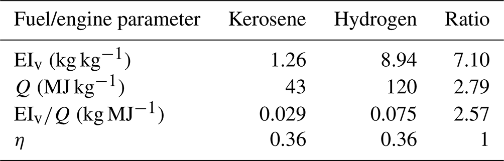
Figure 1 shows that the SA threshold temperature generally increases with rising relative humidity over water (RHwat) on the one hand and with increasing ambient pressure on the other hand. The parts of the curves lying above the solid black line depict the ice-supersaturated cases supporting persistent contrails. In the following, we compare ΘG for hydrogen combustion (blue lines) with those for kerosene combustion (red lines). Using the parameters from Table 1, EIv is around 7.1 and Q is 2.8 times higher for the hydrogen than for the kerosene case (see also Table 1). This leads to an overall increase in the slope of the mixing line (Eq. 1) by a factor of EI 2.6 for fixed η and ambient pressure. As a consequence, ΘG is around 10 K larger for the hydrogen than for the kerosene case (for otherwise fixed conditions). Considering the same atmospheric conditions and ensuring that Ta < ΘG, this will cause significantly higher (peak) plume water supersaturation for the hydrogen case in the early jet phase because the difference is accordingly higher (e.g., Kärcher et al., 2015; Bier et al., 2022). Moreover, droplet formation on aerosol particles will be enabled at higher ambient temperatures as we will show in the Results section.
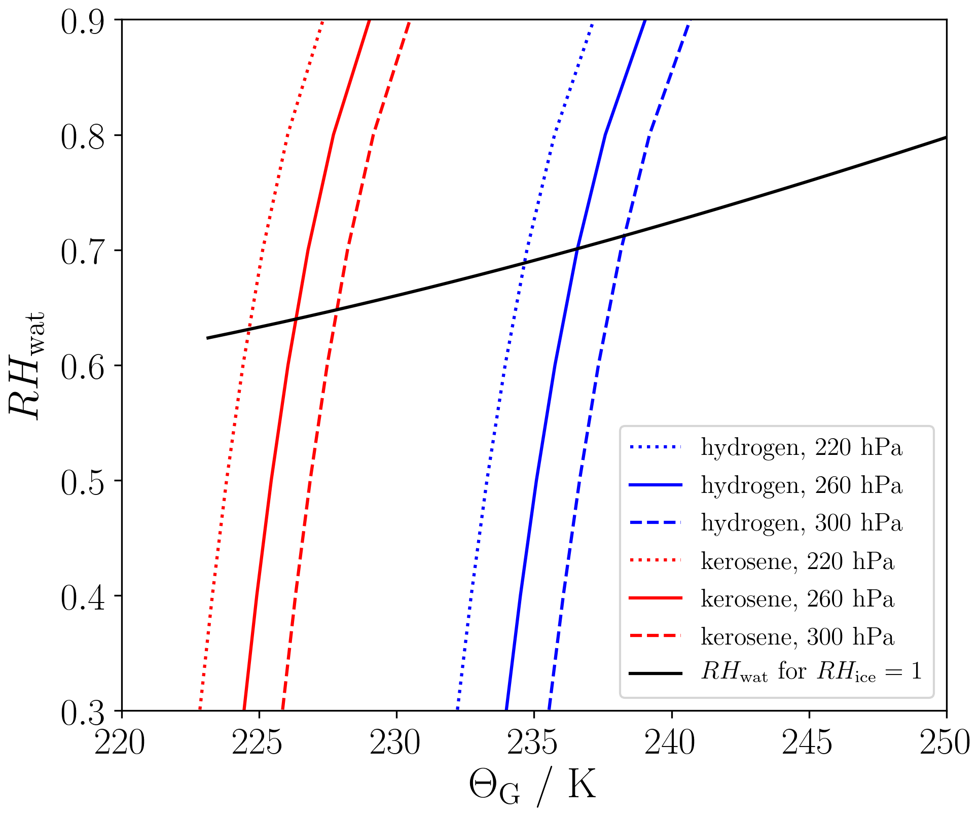
Figure 1SA threshold temperature (ΘG) versus relative humidity over water (RHwat) for three ambient pressures (differentiated by the line style) and for the kerosene (red) and hydrogen (blue) engine parameters as they are defined in Table 1. The solid black line displays those RHwat values that would result in ice saturation assuming an ambient temperature equal to ΘG.
First, Sect. 3.1 gives an overview of the Lagrangian Cloud Module (LCM) and Sect. 3.2 describes the employed trajectory data and plume thermodynamics. Section 3.3 explains the basic contrail formation pathway on ambient particles and the associated extension of the LCM-based box model. Finally, Sect. 3.4 gives an overview of the box model settings and the baseline conditions for the H2 combustion scenario.
3.1 LCM box model
LCM is a particle-based microphysical model that includes aerosol, droplet and ice microphysics (Sölch and Kärcher, 2010). This particle-based approach has several numerical and physical advantages over common grid-based approaches, which are typically used in computational fluid dynamics (CFD). It has been used for the simulation of natural cirrus clouds (e.g., Sölch and Kärcher, 2011), young contrails (e.g., Unterstrasser, 2014) and aged contrail cirrus (e.g., Unterstrasser et al., 2017a). Recently, it has been extended by contrail formation microphysics on soot particles (Bier et al., 2022). Aerosol particles and hydrometeors are described by simulation particles (SIPs). Each SIP represents a certain number of aerosol particles/droplets/ice crystals with the same properties and contains information about the liquid/ice water mass, radius, phase and particle type, among other things. These properties may change due to microphysical processes like hygroscopic growth of aerosol particles and activation into water droplets, condensational droplet growth, homogeneous freezing of supercooled droplets, depositional ice crystal growth, latent heat release, aggregation of ice crystals, sedimentation and radiative effects. In this study, we will consider only those processes that are relevant for contrail formation and exclude aggregation, sedimentation and radiative effects.
3.2 Plume evolution
3.2.1 Trajectory data
In a box model approach, fluid dynamics is not resolved and changes in thermodynamic properties inside the box are externally prescribed. We use the general plume dilution equations, which are described in Sect. 2.3.1 of Bier et al. (2022), to calculate the cooling and expansion of the plume as well as the evolution of the humidity. Based on 3D large-eddy simulations (LESs) using the FLUDILES solver, Vancassel et al. (2014) sampled an aircraft plume with 25 000 trajectories behind the engine of an A340-300 aircraft. Thereby, the temperature evolution T3D,k(t) was tracked for each trajectory indexed by k. As in Bier et al. (2022), we use these data to infer the plume dilution factor by assuming that temperature is a passive tracer:
where K and K are the plume exit and ambient temperatures of the FLUDILES simulation. In the remainder of the text, the subscripts “E” and “a” denote conditions at the engine exit plane and in the atmospheric background, respectively.
In the following, we describe some modifications of the FLUDILES trajectory data set compared to the original one from Vancassel et al. (2014):
-
As in Bier et al. (2022), we introduce a lower limit , and all T3D,k(t) values below this lower limit are set to this value. We choose ϵ=0.2 K such that the implied dilution and plume area are consistent with the area enclosed by the trajectories.
-
We have smoothed the time evolution of T3D,k for each trajectory such that T3D,k becomes a monotonically decreasing function with increasing plume age. This means we set T3D,k(t) := MIN(, T3D,k(t)).
-
In our current model approach, the thermodynamic plume evolution and microphysics are calculated independently for each trajectory, and Bier et al. (2022) find that such an ensemble approach without considering mixing effects among nearby trajectories is not perfect, in particular when the plume is sampled with many trajectories. Hence, we reduce the number of trajectories to ntrsub by merging trajectories that are initially close to each other into a single trajectory. Thereby, we apply a mass-conserving average (that is described in more detail in the Supplement of Bier et al., 2022) to obtain the temporal evolution of the new passive tracer temperature:
where is the weighting factor for mass-conserving averaging and the equation is exemplarily written for one of the ntrsub trajectories.
We have performed sensitivity studies for different ntrsub values. We find that ntrsub=1000 is a reasonable value which still sufficiently resolves the plume heterogeneity and will be used for the analysis in the present paper.
3.2.2 Plume cross-sectional area
The emitted air at the engine exit plane is a mixture of ambient air (going through the engine) and combustion products. The initial plume dilution 𝒞E (i.e., the air-to-fuel ratio) is linked to the exit temperature TE:
This equation follows from the conservation of fuel mass and thermal energy flow. Moreover, J (kg K)−1 is assumed to be an average heat capacity for dry air over the temperature range of interest and the effects of the jet kinetic energy are neglected. The latter assumption is justified when (most) kinetic energy is converted into thermal energy well before the plume has cooled down to temperatures where supersaturation is reached and formation of droplets commences. The overall dilution 𝒞(t) generally increases with plume age due to continuous entrainment of ambient air and is related to the dilution factor 𝒟(t) via
implying 𝒟E=1. Whereas 𝒞 denotes an air-to-fuel ratio, the dilution factor 𝒟 is defined as a fuel-to-air ratio (due to legacy reasons) and decreases with plume age. The word “overall” in the name of 𝒞(t) refers to the fact that this quantity considers the combined effect of dilution occurring in the engine and the free atmosphere. Compared to Eq. (2) we drop the index k from the dilution factor 𝒟k. With this we imply that derivations in this subsection consider the total plume and not individual plume parts represented by a single trajectory.
The flow of the (total) plume mass is defined as
Here, ρ(t) is the air density, A(t) is the plume cross-sectional area (perpendicular to the axial direction) and the total exhaust velocity . The latter quantity Utot(t) is the sum of the absolute value of the aircraft speed, U∞, and jet velocity, Ujet(t), relative to the ambient air. The fuel flow rate (units: kg s−1) is denoted by .
Applying Eq. (6) at the engine exit plane and at any other time for a fixed fuel flow rate, plugging in Eq. (5), using the ideal gas law, and assuming isobaricity, we obtain the following relation:
Note that Eq. (16) in Bier et al. (2022) shows a similar relation; however it misses the ratio of the velocities. The same holds for their Eq. (15). This term accounts for the fact that the plume is compressed/stretched due to the axial divergence of the jet. This clearly affects how the cross-sectional plume area changes over time. However, this divergence effect does not change the volume of the considered air parcel; it only distributes its mass over a segment with a changing extent along the axial direction. The volume of the plume changes only due to the entrainment of ambient air (reflected by the dilution factor 𝒟) and through associated density changes (reflected by the temperature ratio). Introducing an effective area
Eq. (7) can be written as
The effective area is the cross-sectional area that is reached when the exhaust plume is (theoretically) decelerated from Utot(t) to U∞ in a volume-preserving manner. Since we provide all quantities in terms of “per meter of flight path”, the effective area is the appropriate quantity that is representative of the volume of the plume at a certain age. Note that Eq. (9) has the same form as Eq. (16) in Bier et al. (2022). The only difference is that it uses the effective plume cross-sectional areas instead of the real physical ones. In our case, U∞=250 m s−1 and m s−1. Hence, the ratio is 1.92.
The fuel consumption per meter of flight path mC can be computed by
mC is the amount of fuel that is burned per unit length along the flight direction. The amount of a corresponding combustion product per flight distance is then, e.g., (where EIPT is the emission index of an assumed passive tracer). However, we have to keep in mind that mPT only specifies the amount of the tracer in a segment where the jet velocity approached 0. At the engine exit plane, the total tracer amount would be lower by a factor of γU.
In the preceding paper of Bier et al. (2022), formulas were expressed in terms of fuel consumption and never in terms of the fuel flow rate. There, the symbol mF was used for the fuel consumption. In the present paper, this is replaced by mC in order to avoid confusion with the fuel flow rate .
Even though we made the comment that the derivations here consider the total plume, they are also valid for individual plume air parcels represented by a trajectory. The FLUDILES simulation data feature an initial plume temperature profile with a smooth radial transition between the plume and the environment instead of a step at the plume edge. Hence, trajectories in the outer plume regions start with and 𝒟k(t) < 1.0. In principle, one could assign a trajectory-specific value of γU to each trajectory. The fraction of trajectories having a γU value much smaller than the default is rather small. Hence, we apply a bulk-correction factor of γU=1.92 to ensemble mean values (instead of applying individual correction factors to each trajectory and then performing a suitable mass-weighted averaging/summation to trajectory ensemble data). This simplification leads only to minor quantitative deviations.
As written above, Bier et al. (2022) missed including the term γU in the computations of plume area and fuel consumption. However, the implications of this are not overly serious. The time evolution of intensive quantities in the box model is not affected by this oversight. Only in the final step of translating ice crystal number concentrations into a total number of ice crystals Nice per flight distance does one have to include the term γU. However, for quantities like the apparent ice emission index (AEI) or the activation fraction, as shown in the figures of Bier et al. (2022), the term γU is canceled out and the displayed figures are all unaffected by our oversight. For the sake of clarity, we want to note that the simulations of kerosene contrails discussed in Sect. 4.4 of the present study are computed with the correct formulas.
3.3 Contrail formation pathway on entrained ambient particles
In our study, we assume H2 combustion with soot-free emissions. Moreover, we exclude the potential formation of ultrafine particles due to lubricant oil vapor, which will be separately discussed in Sect. 5. Hence, contrails will solely form on ambient background particles in suitable atmospheric conditions (e.g., Kärcher et al., 1996, 2015). The microphysics of contrail formation on soot particles, as implemented in the LCM, has been described in detail by Bier et al. (2022). These microphysical processes are mostly also relevant for contrail formation on ambient particles and will be summarized briefly in this section. We focus our description on additional aspects for H2 contrails and the associated extensions in the LCM-based box model. The major difference besides the chemical composition is the fact that ambient particles are continuously entrained instead of releasing a fixed number of emitted soot particles. Finally, we introduce an alternative activation criterion and an extended homogeneous freezing parameterization. This accounts for the better solubility of the majority of UT particles compared to engine soot.
3.3.1 Ambient aerosol particle properties
We prescribe background particles as an ensemble that is characterized by a log-normal size distribution with a geometric mean dry radius (), a geometric width (σaer) and a number concentration (naer). Moreover, we specify the hygroscopicity parameter (Petters and Kreidenweis, 2007). The parameters are varied mostly independently of each other, representing different types of ambient aerosol particles and accounting for their natural variability.
According to the classical microphysical pathway of contrail formation with the liquid transition phase (e.g., Kärcher et al., 2015; Bier et al., 2022), we consider only CCN or partially soluble mixed particles (i.e., an insoluble core and a hydrophilic coating), where we assign the latter simply to “weakly soluble particles”. We exclude heterogeneous ice nucleation on insoluble particles, since measured and modeled number concentrations of ice nuclei (IN) in the UT are typically several orders of magnitudes lower than those of CCN (e.g., Rogers et al., 1998; Beer et al., 2022). Even though IN may have important effects on natural cirrus cloud properties (e.g., Hendricks et al., 2011), we expect a negligible contribution to the overall contrail ice crystal formation. Insoluble but still wettable particles like uncoated soot and oil droplets could also be treated by adsorption activation theory. This is based on standard Köhler theory but uses a specific description of the water activity that accounts for adsorption processes. In particular, the Frenkel, Halsey and Hill (FHH) adsorption approach (Sorjamaa and Laaksonen, 2007; Kumar et al., 2009) is able to treat multilayer adsorption of water vapor onto insoluble particles and should be considered in future studies.
For simplicity, we assume that the entrained ambient particles are initially completely dry, i.e., without any previous environmental hygroscopic water uptake. We allow for condensational growth of the entrained aerosol particles not only in water-supersaturated conditions but also at plume relative humidities lying between the deliquescence relative humidity (DRH) and water saturation. Thereby, DRH is the minimum threshold relative humidity that allows for hygroscopic water uptake by a given substance.
3.3.2 Entrainment of ambient particles
Aerosol particles from the environment are continuously entrained into the plume. The background aerosol abundance is specified in terms of an aerosol background number concentration naer.
As a next step, we quantify the number of aerosol particles Naer(t) (here per flight distance) that are present in the expanding plume.
The ratio of densities in the first line accounts for the fact that during an adiabatic entrainment process, the mixing ratio is conserved and not the concentration. Moreover, we assume that the initial plume is void of any aerosol particles, which implies that any aerosol particle sucked into the aircraft engine is destroyed. Hence, the plume area at the engine exit is subtracted (second term in the first line). The further re-formulations assume isobaric conditions and use the ideal gas law and the definition of the effective area (Eq. 9).
If we were to also prescribe aerosol particles in the initial plume (with identical properties to those in the environment), results would not change too much as their contribution to the total aerosol particle number would become smaller and smaller while the plume expands (this case is easily treated by removing “−1” from the term “”).
The number of particles being entrained into the plume during one time step Δt is then given by
In every time step, a new SIP ensemble representing these newly entrained particles is created. Only in the initial stages of the simulation when RHwat is still below DRH do no new SIPs have to be created as aerosol particles inside the plume are still dry. In this case, it is sufficient to only increase the SIP weight (i.e., the number denoting how many real particles are represented by a SIP).
Clearly, the continuous creation of new SIPs would cause huge values of NSIP and lead to computationally expensive or even unfeasible simulations. Hence, we apply a SIP merging algorithm if the overall SIP number NSIP gets too large (see Appendix A).
Moreover, we found that T3D happens to increase in certain (short) segments along several plume trajectories. This implies that the cross-sectional area represented by the trajectory shrinks (i.e., ) and a negative value of ΔNaer(t) follows. To inhibit such an unwanted detrainment of particles and hydrometeors, we have smoothed our trajectory data such that the dilution C(t) is a monotonically increasing function with time (see Sect. 3.2.1).
3.3.3 Diffusional growth and freezing
For spherical droplets, the single-droplet mass growth equation is given by Kulmala (1993) as
where r is the wet aerosol or droplet radius ev is the partial vapor pressure. Lc denotes the specific latent heat for condensation and evaporation, Dv the binary diffusion coefficient of air and water vapor, K the conductivity of air, Rv the specific gas constant of vapor, and T the temperature. The transitional correction factors βm and βt are calculated according to Eqs. (A4) and (A5) of Bier et al. (2022) based on Fuchs and Sutugin (1971). Note that there is a transcription error in the previous study, and the denominators of both Eq. (A4) and Eq. (A5) miss the term “+1”. With this correction, βm and βt tend towards 1 for small Knudsen numbers, as intended. The quantity eK,wat is the product of the saturation vapor pressure over a flat water surface esat,wat and the equilibrium saturation ratio over a solution droplet surface SK. As in Bier et al. (2022), we calculate SK using the κ-Köhler equation (Petters and Kreidenweis, 2007):
where the first term is the activity of water (awat) and the exponential expression is the Kelvin term. rd is the particle dry radius, κ the hygroscopicity parameter, the surface tension of the solution droplet, ρwat the mass density of water, Mwat the molar mass of water and R the universal gas constant. The surface tension typically increases with decreasing awat for salt solutions due to negative adsorption and increases with decreasing awat for acidic solutions due to positive adsorption. Since we do not prescribe specific aerosol particle species but only the hygroscopicity parameter in the present study, we approximate with the surface tension of pure water droplets and use the polynomial expression by Hacker (1951) as in Bier et al. (2022). Hence, a slight error is caused in the Kelvin term for more concentrated solution droplets.
The entrained ambient aerosol grows by condensation if RHwat is larger than the deliquescence relative humidity (DRH). As long as the entrained particle is completely dry, SK is not applicable, since r=rd. Therefore, we set SK to a value that is slightly lower than RHwat for the first time step with condensation. This causes the particle to grow hygroscopically so that r > rd in the next time step, and then SK is calculated according to Eq. (14). During the subsequent plume evolution, the wetted particle/droplet grows further due to condensation if RHwat > SK or shrinks due to evaporation if RHwat < SK according to Eq. (13). In Bier et al. (2022), the soot particles were considered to be activated into water droplets if the wet radius exceeded the critical radius, which is the radius at the maximum of SK. In the present study, we consider aerosol particles to be activated into water droplets if the activity of water has exceeded a critical value to ensure sufficient water uptake for freezing. Once an aerosol particle has been activated into a droplet, it can freeze into an ice crystal if the plume temperature drops below the homogeneous freezing temperature of that solution droplet (Tfrz). For the calculation of Tfrz, Bier et al. (2022) follow the approach of Kärcher et al. (2015) and Riechers et al. (2013) assuming pure water droplets. We extend this approach by including a simple correction term, based on the parameterization of O and Wood (2016), to account for the decrease in Tfrz due to the solution effect (e.g., Koop et al., 2000). Further details are described in Appendix B.
The depositional growth of the ice crystals formed is calculated according to Eq. (7) of Bier et al. (2022), which is based on Mason (1971). Note that there is a transcription error in that equation, where the correction term occurs twice in the mass diffusion term and should be removed in the denominator.
3.4 Model settings and baseline parameters
Table 2 summarizes our baseline initial and background conditions for H2 combustion as well as the ambient particle properties and model setup parameters. We prescribe an ambient temperature Ta of 225 K, ambient pressure pa of 260 hPa and relative humidity over ice RHice,a of 120 %. We define a water vapor mass emission index EIv and specific combustion heat Q that are typical of hydrogen propulsion (Table 1). We set the propulsion efficiency, engine exit temperature and initial plume area to the same values as in Bier et al. (2022). The fuel and engine parameters EIv, Q, η and TE are kept constant for all sensitivity studies even though they can slightly change with ambient conditions; see Sect. 5.2. We determine the initial plume dilution 𝒞E and the fuel consumption mC according to Eqs. (4) and (10). Since AE is the area of one engine nozzle exit plane (based on the FLUDILES data for the four-engine A340-300 aircraft and kept constant in this study), our mC value is representative of a single engine and would be 4 times larger for the whole aircraft. Thus, we simulate contrail formation behind a single aircraft engine. The 𝒞E and mC values listed in Table 1 are given for the atmospheric baseline Ta and pa values. Note that 𝒞E is larger and mC lower by a factor of 2.8 compared to kerosene combustion because Q is accordingly higher (with the relations 𝒞E∼Q and ). An analogous kerosene setup would have baseline values 𝒞E≈76 and mC≈3.1 g m−1.
Table 2Baseline parameters for our LCM box model studies. The fuel, engine properties and exit conditions refer to H2 combustion. In addition to the entrained ambient particle properties, we provide the baseline soot particle properties for a comparison of H2 with conventional contrails.
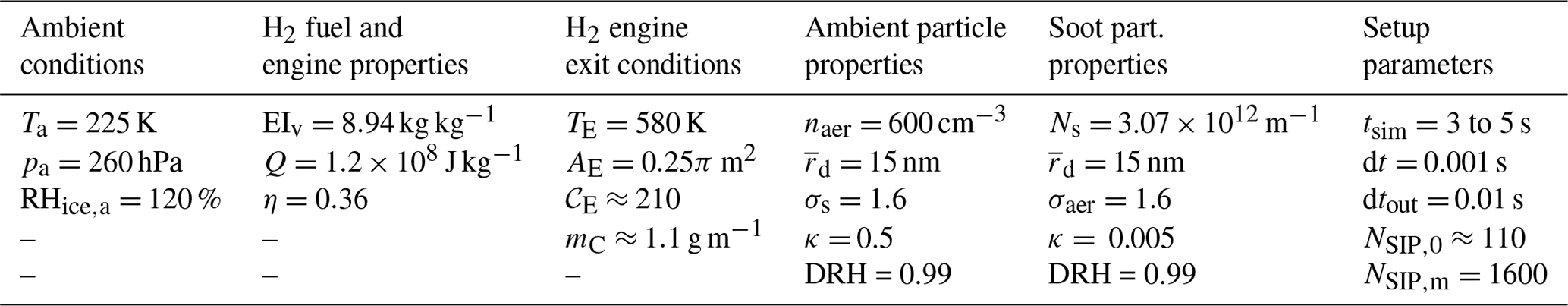
We prescribe ambient particles with a mono-modal log-normal size distribution. We set the geometric mean dry radius () to 15 nm and geometric width to 1.6, representing a typical Aitken aerosol mode in the UT (e.g., Brock et al., 2021). We define an aerosol number concentration (naer) of 600 cm−3, which lies well between the observed values for Aitken- and accumulation-mode particles (e.g., Minikin et al., 2003; Borrmann et al., 2010). We set the hygroscopicity parameter κ to 0.5, which is, e.g., a typical value of ammonium sulfate particles (Liu et al., 2014). Peng et al. (2022) provide a large data set for DRH of different atmospheric compounds (e.g., see their Table 1). Even though many inorganic compounds have a DRH significantly below 1, we set our baseline DRH very close to water saturation. The reason for that will be discussed in Sect. 5.2. For a comparison with conventional contrails, we also provide associated soot particle properties in Table 2.
For any ambient particle ensemble, we use around 110 SIPs to represent its log-normal size distribution. For this, we use the algorithm described in Unterstrasser and Sölch (2014), which has favorable numerical convergence properties (Unterstrasser et al., 2017b). Each simulation contains an ensemble of box model runs for 1000 different trajectory data as described in the previous section. The runs are performed independently of each other for each trajectory. The standard simulation time is 3 s; the numerical time step is 0.001 s. For some simulations with Ta < 220 K, we extend the simulation time to 5 s, since the time period when droplet and, hence, ice crystal formation occurs is longer than 3 s. Typically, droplet and ice formation comes to a halt well before a plume age of 5 s, and hence, the ice crystal number does not increase anymore.
In this section, we first analyze the temporal evolution of thermodynamic and microphysical H2 contrail properties for our baseline case (Sect. 4.1). We then investigate the impact of atmospheric conditions on those properties in Sect. 4.2. In Sect. 4.3, we analyze the influence of ambient aerosol particle properties on contrail ice crystal formation prescribing either one or two co-existing aerosol particle ensembles. Finally, we compare our results with conventional kerosene contrails in terms of ice crystal number and optical thickness in Sect. 4.4. The thermodynamic and microphysical properties are either averaged or summed up over all box model trajectories obeying a mass-conserving weighting as each trajectory may represent a different share of the plume at later times. In this study, we always display our microphysical properties in units (number or mass) per flight distance.
4.1 Temporal evolution of contrail properties for the baseline case
Figure 2 shows the temporal evolution of thermodynamic and microphysical properties for our baseline case defined in Table 2. The mean plume temperature (Fig. 2a) decreases with increasing plume age due to continuous mixing of the exhaust with ambient air approaching the ambient temperature. Accordingly, the plume dilution and, therefore, the effective plume area increase, the latter from around 1.5 to 540 m2 after 3 s. The mean relative humidity over water RHwat (Fig. 2b) surpasses the deliquescence relative humidity after around 0.2 s and reaches its maximum of around 220 % after 0.4 s. Compared to a plume behind a conventional aircraft (e.g., see Fig. 2 in Bier et al., 2022), our maximum RHwat and accordingly RHice values are substantially higher, since the difference between the ambient and the SA threshold temperature is larger (the SA threshold temperature is around 10 K higher for H2 than for kerosene combustion; see Sect. 2.2).
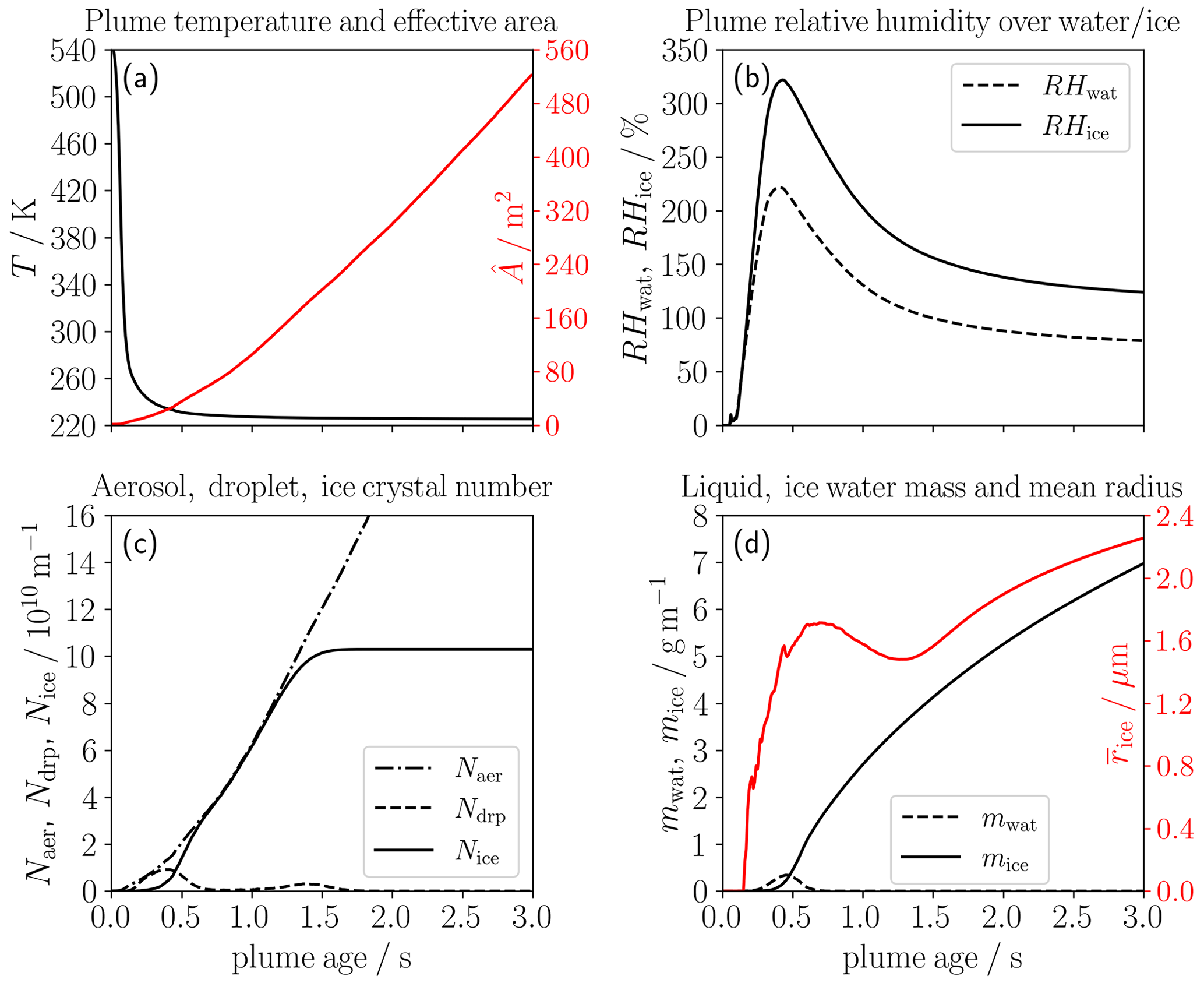
Figure 2Temporal evolution of thermodynamic and microphysical properties in a single-engine plume for the baseline case: the panels show the (a) temperature (black) and effective cross-sectional area (red and labels on the right axis), (b) relative humidity over water (dashed) and ice (solid), (c) number of aerosol particles entrained into the plume (dash-dotted) and number of droplets (dashed) and ice crystals (solid) per flight distance, and (d) liquid (dashed black) and ice water mass per flight distance (solid black) and mean radius of the ice crystals (red and labels on the right axis).
Figure 2c shows the accumulated number of aerosol particles entrained into the plume (Naer), the number of formed droplets (Ndrp) and the number of ice crystals (Nice). Naer increases nearly linearly with time, reaching values of around 1.15 × 10¹¹ and 3.07 × 10¹¹ m−1 after 1.5 and 3 s, respectively. This is different to exhaust species like soot particles, since they typically form right behind the engine exit (when plume relative humidity is still low and no activation occurs) and their emitted number (per flight distance) is then assumed to be constant over time.
The Naer values are mainly controlled by the ambient aerosol number concentration (naer) and the plume area expansion. The first aerosol particles activate into water droplets (dashed line) after RHwat surpasses the DRH in the corresponding trajectories. A few tenths of a second later, they freeze into ice crystals (solid line) once plume temperature falls below the homogeneous freezing temperature of those droplets. Later on (at plume ages between around 0.6–1.1 s), Nice is very close to Naer. This means that basically all entrained aerosol particles nearly instantaneously form droplets and freeze. After 1.5 s when the mean RHwat falls below approximately 95 %, no further droplets and ice crystals form. Therefore, Nice stays constant afterwards at 1.04 × 10¹¹ m−1. Some of the droplets (small peak in Ndrp at around 1.4 s) cannot freeze, and they evaporate afterwards. This is because the homogeneous freezing temperature of those droplets, which either are too small or have water activity that is too low, is not reached. The ice crystals grow by deposition so that the ice water mass (mice) continuously increases (Fig. 2d). The mean ice crystal radius (red line) tends to increase over time and finally reaches a size of around 2.2 µm. The decrease in between 0.6 and 1.3 s is because more and more of the smaller droplets manage to freeze into ice crystals and, hence, the mean ice crystal size drops in that time period. Since the plume is still ice-supersaturated (solid line in Fig. 2b) after 3 s, mice and would increase even further.
4.2 Impact of atmospheric properties
Here, we investigate in detail the impact of ambient temperature on the plume thermodynamical and microphysical contrail properties. Moreover, we analyze the influence of ambient pressure and relative humidity over ice. We prescribe our baseline ambient aerosol particle properties and keep them constant in this section. Note that a fixed aerosol number concentration for varying atmospheric parameters (in particular pressure) is an idealized assumption in the following sensitivity studies.
4.2.1 Influence of ambient temperature on temporal evolution of thermodynamic and contrail properties
Figure 3 highlights the strong impact of ambient temperature Ta on contrail ice crystal formation. As shown in Fig. 3a, the plume temperature at a given plume age is certainly lower in a colder environment and finally approaches the corresponding Ta value. The peak mean relative humidity over water (displayed in Fig. 3b) increases with decreasing Ta (reaching values of around 350 % and 550 % for Ta values of 220 and 215 K, respectively). The large increase for low Ta values is due to the non-linearity between saturation vapor pressure and temperature. The relative humidity over ice behaves accordingly (not shown).
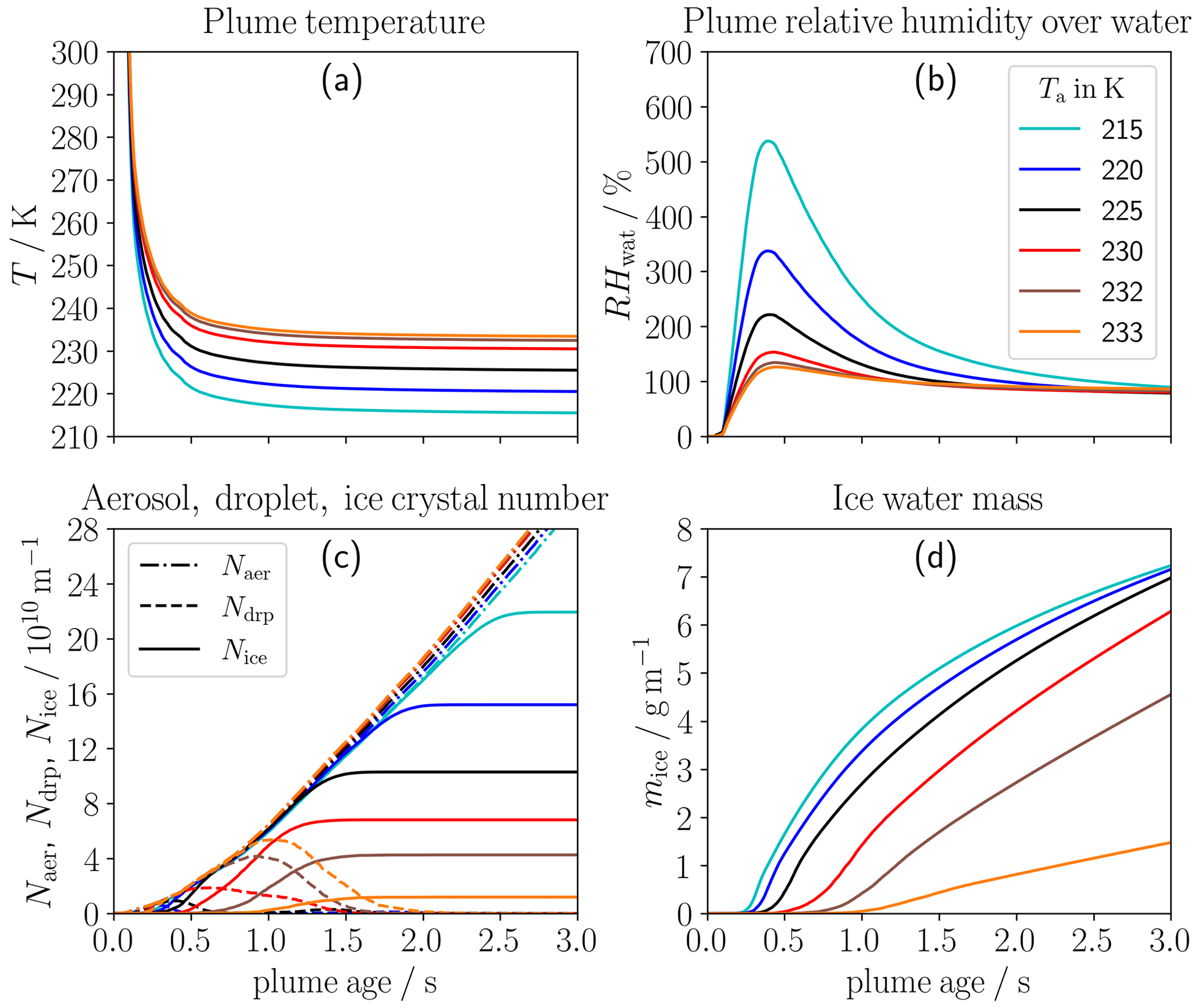
Figure 3Impact of ambient temperature (Ta) on the temporal evolution of thermodynamic and microphysical properties in a single-engine plume: the panels show the (a) temperature, (b) relative humidity over ice, (c) number of aerosol particles entrained into the plume (dash-dotted) and number of droplets (dashed) and ice crystals (solid) per flight distance, and (d) ice water mass per flight distance. The colors represent the different Ta values as defined in the legend.
The slight change in the evolution of Naer is a consequence of our model setup with a fixed aerosol number concentration and the varying plume air density with temperature (at fixed ambient pressure). In general, the droplet formation is basically controlled by the time period where RHwat is above DRH such that water can condense on the entrained aerosol particles. (Note that the evolution in RHwat and, therefore, this time period vary with each trajectory, and here we only display the ensemble mean quantity.) This mean time period for possible droplet and ice crystal formation substantially increases with decreasing ambient temperature (e.g., from 0.15 s up to 2.8 s for Ta= 215 K). This means that ice crystal formation is initiated earlier and comes to a halt later (see solid red and blue lines in Fig. 3c) compared to the baseline case. Moreover, nearly all formed droplets freeze very quickly into ice crystals so that Ndrp approaches zero. For these reasons, the final ice crystal number strongly increases with decreasing Ta over the whole temperature range (see also Fig. 4). This is different to what we find for conventional soot contrails as all soot particles turn into ice crystals if Ta is several kelvins below the SA threshold temperature (e.g., Kärcher et al., 2015; Bier and Burkhardt, 2019; Bier et al., 2022). Yet, any further reduction in Ta does not lead to more ice crystals in the conventional case. Moreover, the peak plume RHwat values are substantially higher for H2 than for kerosene combustion in the same ambient conditions. Therefore, droplet and ice crystal formation on ambient particles is controlled more strongly by the time period in which the plume is water-supersaturated than by the maximum water supersaturation.
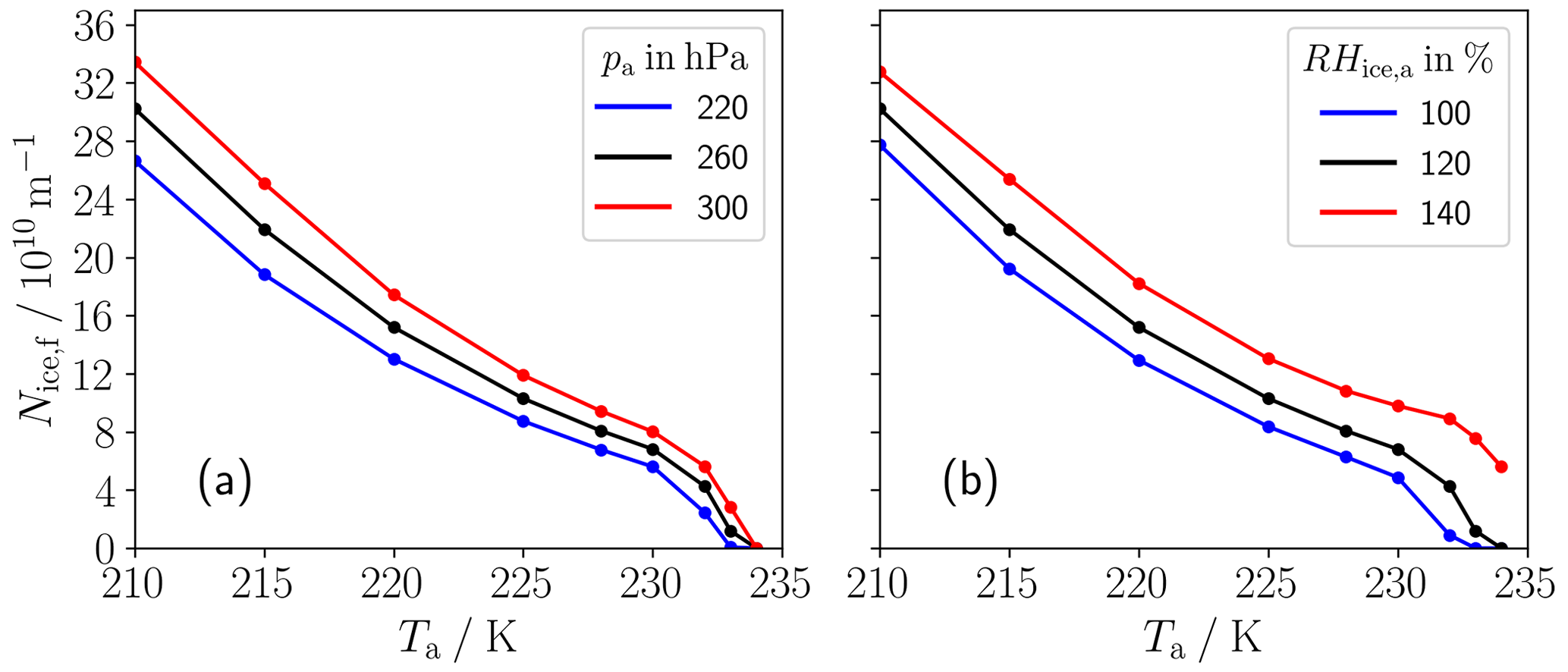
Figure 4Final ice crystal number per flight distance (Nice,f) in a single-engine plume versus ambient temperature for (a) three different ambient pressures (pa) and (b) three different ambient relative humidities over ice (RHice,a). The black line in both panels always refers to the baseline pa and RHice,a values. Nice,f is given at a plume age of 3 s for Ta≥ 215 K and at a plume age of 5 s for Ta= 210 K.
For higher ambient temperatures (Ta≥ 230 K), many droplets cannot freeze into ice crystals and evaporate thereafter (which is indicated by declining Ndrp at nearly constant Nice). This is because the homogeneous freezing temperature of the smaller and/or more concentrated solution droplets is below the plume/ambient temperature. Hence, the final ice crystal numbers are decreased further in addition to the fact that the time period for possible droplet formation is lower. The decrease in Nice with increasing Ta becomes stronger for Ta≥ 232 K (see also Fig. 4), and for Ta= 233 K, only a few large droplets can form ice crystals. For higher ambient temperatures no ice crystal formation occurs anymore. This means that for H2 combustion, the freezing temperature is typically smaller than the SA threshold temperature and becomes a more limiting criterion for contrail formation. Yet, the SA threshold temperature is still relevant, as its difference from the ambient temperature determines the peak and time period of water supersaturation in the plume. The ice water mass (shown in Fig. 3d) in general increases with decreasing ambient temperature. The strong increase between Ta values of 230 and 233 K is mainly due to the increase in Nice.
In the following sections, we will focus our analysis on the final number of ice crystals formed (Nice,f), since the young-contrail ice number mostly impacts the further contrail (cirrus) properties and radiative forcing (e.g., Bier et al., 2017; Burkhardt et al., 2018; Bier and Burkhardt, 2022). In contrast, the initial ice water mass and mean ice crystal radius were shown to have a low impact on the contrail life cycle in the dispersion phase (e.g., Unterstrasser and Gierens, 2010), but the size distribution of the contrail ice crystals formed can strongly impact the sublimation loss of ice crystals during the vortex phase (e.g., Unterstrasser, 2014). The latter will be investigated in future studies.
4.2.2 Final ice crystal number
Figure 4 displays Nice,f versus ambient temperature Ta for (a) three different pressure pa values and (b) three different values of ambient relative humidity over ice RHice,a. Note that our parameter settings are simplified in the sense that some combinations of parameter values are not realistic for the atmosphere (e.g., the lowest Ta value at the highest pa value). Compared to the previous subsection, we now include a further case with Ta= 210 K (that requires a longer simulation time, since the period when the plume is water-supersaturated is longer than 3 s). This case emphasizes the enhanced increase in Nice,f with decreasing Ta for very cold conditions and is consistent with the findings by Ström and Gierens (2002). Nice,f is increased for a higher ambient pressure because the slope of the mixing line G, defined by Eq. (1), is larger for a higher pressure. Moreover, Fig. 4b shows an incline of Nice,f with increasing RHice,a. Both the increased G and the higher RHice,a lead to higher peak plume relative humidities and enlarge the time period for possible droplet and subsequent ice crystal formation. Interestingly, this increase is quite strongly pronounced for the highly ice-supersaturated case (red line) at ambient temperatures between 230 and 234 K (and for 234 K ice crystals can only form at all for this case). This is because the droplet freezing is mainly limited by the droplet size in that Ta range, and for the high-RHice,a case, more larger droplets can form that turn into ice crystals.
Finally, ambient temperature is the parameter that most influences the number of contrail ice crystals formed, while the impact of ambient pressure and relative humidity is clearly smaller. This behavior is similar to the conventional case with kerosene combustion despite the very different temporal evolution in the exhaust particle number concentration.
4.3 Sensitivity of ice crystal number to ambient aerosol particle properties
In this section, we investigate the impact of ambient aerosol particle properties on the (final) number of ice crystals formed in H2 contrails. We prescribe one aerosol particle ensemble (single mode) in Sect. 4.3.1 (as in the previous analysis) and two co-existing aerosol particle ensembles in Sect. 4.3.2.
4.3.1 Studies with a single-aerosol particle ensemble
Figure 5 shows the variation in Nice,f with different aerosol particle properties. The sensitivities are always shown for three ambient temperatures Ta (differentiated by the color). In general, we see an increase in Nice,f with decreasing Ta for any particle property combination, being consistent with the findings in the previous section. Figure 5a shows that Nice,f increases with increasing aerosol number concentration naer. This increase becomes weaker for higher naer (⪆ 200 cm−3) values. This is due to the enhanced competition for plume water vapor between the growing droplets/ice crystals for increased aerosol number concentrations.
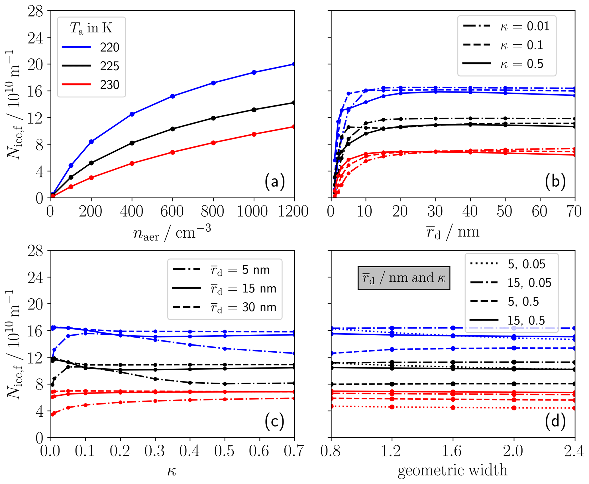
Figure 5Final ice crystal number per flight distance (Nice,f) in a single-engine plume depending on different aerosol particle properties assuming uni-modal size distributions for three ambient temperatures (Ta) (different colors defined in legend a): Nice,f is shown versus the (a) ambient aerosol number concentration, (b) geometric mean dry radius () for three solubility values (see line style in legend b), (c) hygroscopicity parameter (κ) for three values (see line style in legend c) and (d) the geometric width of the size distribution for four different –κ combinations as displayed in the legend.
Next, we analyze the importance of the mean dry radius of the aerosol size distribution and the hygroscopicity parameter κ. Typically, the ice crystal number strongly increases with increasing mean dry size for 10 nm and then stays nearly constant (see Fig. 5b). The increase is mainly due to the Kelvin effect; i.e., larger aerosol particles are easier to activate into water droplets, since they require lower plume water supersaturations and grow more quickly into water droplets (e.g., Bier et al., 2022).
Figure 5c shows the dependence of Nice,f on κ. For Ta= 230 K, Nice,f slightly increases for a larger κ for all three values as indicated in the legend. For the lower-Ta cases, the variation in Nice,f with and κ is more complex. For the small-sized particles (dash-dotted lines), there are two counteracting effects: Nice,f increases with a rising hygroscopicity parameter for κ < 0.1, since more soluble particles can more easily form water droplets. On the other hand, Nice,f subsequently decreases. This is because some of the droplets cannot freeze into ice crystals, since their water activity is lower due to the enhanced solution effect for higher κ, and, therefore, the homogeneous freezing temperature is significantly decreased (see Fig. B1 in the Appendix). For the other cases, Nice,f hardly changes with the solubility and mean aerosol particle size.
We also analyze in Fig. 5d the impact of the geometric width of the aerosol size distribution for four different –κ combinations as displayed in the legend. Our results imply a very low sensitivity of Nice,f to the geometric width.
In conclusion, the sensitivity of the ice crystal number to and κ is low for aerosol particles with a large mean dry size. For the small-sized particles, we find a quite complex variation in Nice,f with κ, mainly for low ambient temperatures, due to various counteracting effects.
4.3.2 Studies with two co-existing aerosol particle ensembles
So far, the aerosol particles have been prescribed with a single log-normal size distribution and a fixed hygroscopicity value. In the present section, we prescribe two co-existing ambient aerosol particle ensembles and analyze contrail ice crystal formation for two ambient temperatures. The given naer value is the total number concentration of both aerosol ensembles. We restrict our analysis to cases where each ensemble has a number concentration of 0.5⋅naer. We consider nucleation-mode ( 3 nm), Aitken-mode ( 15 nm as in our baseline case) and accumulation-mode ( 50 nm) particles. The given mean dry sizes of the single modes are prescribed consistently with typical observed UT geometric mean diameters over the Atlantic and Pacific oceans within the ATom campaign (see Fig. 12 of Brock et al., 2021). Moreover, we consider well-soluble (κ= 0.5) particles like inorganic salts and weakly soluble ambient particles (κ= 0.05) like organic species or aviation soot. We restrict our analysis to a scenario where the two co-existing particle ensembles always differ in either their mode (in our case ) or the solubility κ. Moreover, we compare the total Nice of the two aerosol particle ensembles with a reference case, which uses a single aerosol population with the same value of naer and the average and κ values of the two particle ensembles.
The first two rows of Fig. 6 show the temporal evolution of Nice with a fixed naer of 600 cm−3. First, we analyze the contrail ice number evolution for bi-modal aerosol size distributions with the same κ value (first row). Panel (a) shows that Nice for the Aitken-mode particle is at the end around 50 % larger than that for the nucleation-mode particle for both temperatures. This is because, for a given plume relative humidity, the larger particles can better activate into water droplets (and freeze thereafter) than the very small nucleation-mode particles due to the Kelvin effect. Moreover, the total ice crystal number is at the end around 10 % lower than the reference Nice. Considering the Aitken and accumulation mode in panel (b), Nice between the two particle ensembles is quite similar and for Ta=230 K nearly identical. This is consistent with the findings for a single particle ensemble where the variation in the ice crystal number for 10 nm is low (see Fig. 5b). For the same reason, the total and reference Nice values are close to each other.
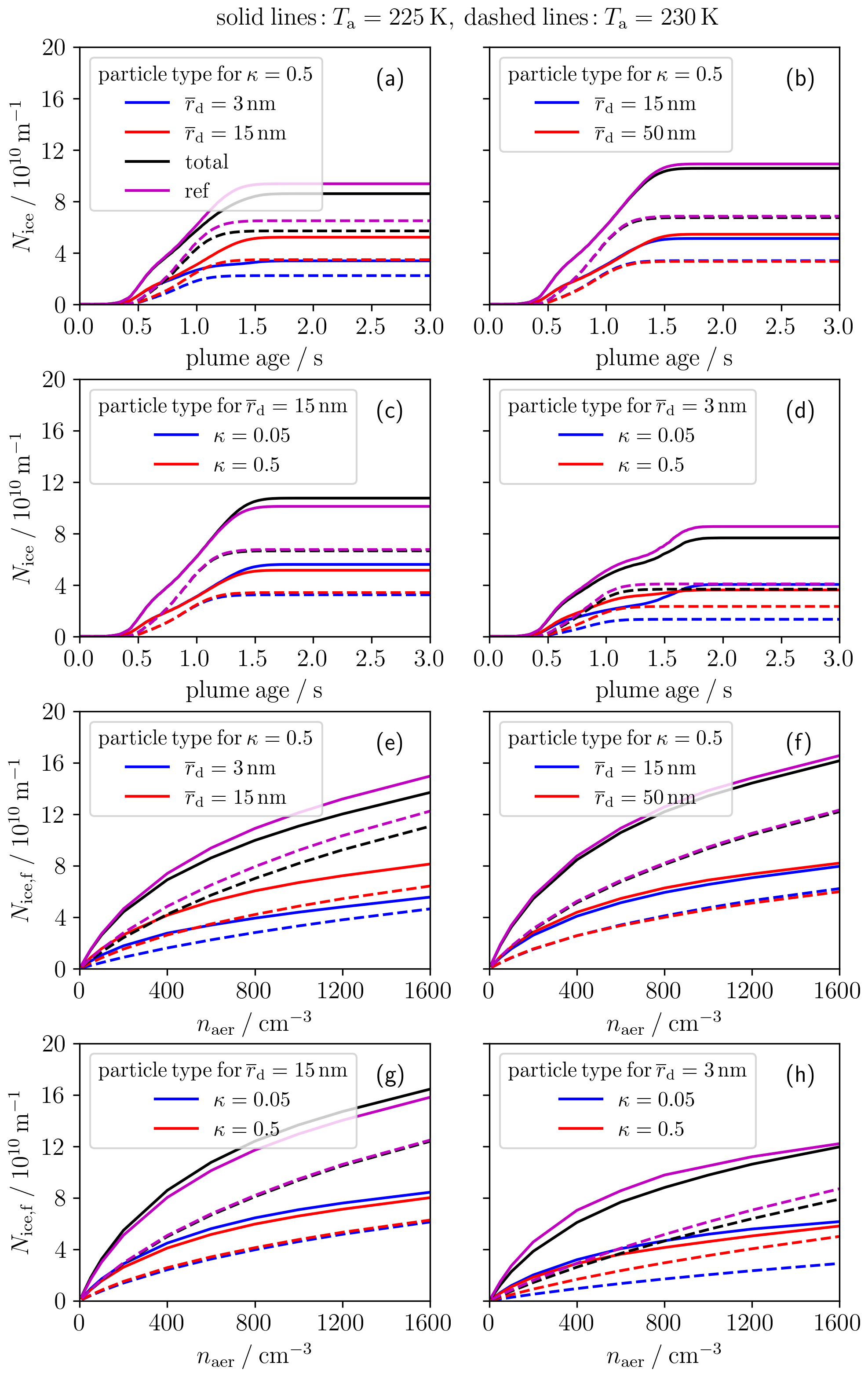
Figure 6Ice crystal number per flight distance for two co-existing ambient aerosol particle ensembles: all results are shown for two ambient temperatures (225 K solid and 230 K dashed). The first two rows show the temporal evolution of ice crystal number Nice and the last two rows the final ice crystal number Nice,f (at a plume age of 3 s) versus the total ambient aerosol number concentration of both ensembles. The blue and red lines depict the Nice of the single-aerosol ensembles and the black lines the sum of both co-existing ensembles. The magenta lines represent reference cases from simulated single-aerosol particle ensembles prescribing average quantities of the two co-existing ensembles. Panels (a, e) and (b, f) show results for a bi-modal aerosol size distribution (with mean dry radii as displayed in the legends) for a fixed hygroscopicity parameter κ= 0.5. The other panels show results for two aerosol particle ensembles with a different solubility (κ= 0.05 and 0.5) but a fixed , namely 15 nm in panels (c) and (g) and 3 nm in panels (d) and (h).
Now, we investigate the ice crystal formation for particle ensembles with two different solubility characteristics but the same (second row). For Ta= 230 K, Nice for the weakly soluble particles is lower than for the well-soluble particles. This is because the less hygroscopic particles are harder to activate and/or cannot grow to sufficiently large droplet sizes in order to freeze into ice crystals. Hence, the total ice crystal numbers are slightly reduced (by around 5 %–10 %) relative to the reference ice numbers. For Ta= 225 K, Nice is at the end lower for κ=0.5 than for κ=0.05 and the total ice number is lower than the reference ice number, contrary to the high-Ta cases. This is due to the decrease in Tfrz for droplets with a higher solution effect (lower awat), as explained in Sect. 4.3.1 and shown in Fig. 5c.
The last two rows show the final ice crystal numbers (Nice,f) for the same aerosol particle ensembles as in panels (a)–(d) but for different aerosol number concentrations. Basically, we see a similar trend for the ice crystal numbers of the single ensembles and the reference case to that in the panels above throughout the whole naer range. In general, the increase in Nice,f with increasing naer becomes weaker for higher naer, in particular for the low-Ta cases. This is consistent with the findings for a single-aerosol ensemble (as already shown in Fig. 5a). The flattening in Nice,f is pronounced most strongly for the nucleation mode and the weakly hygroscopic particles. Again, the total Nice,f of the two particle ensembles is nearly always reduced compared to the reference Nice,f of the single average particle ensemble except for the low-Ta cases in panel (g) and (h).
Finally, we find the largest differences between the total ice crystal number of the co-existing particle ensembles and the associated average single particle ensemble for the cases where nucleation-mode particles are involved. This is mainly due to the non-linearity between the (final) contrail ice crystal number and mean dry size for those very small aerosol particles.
4.4 Comparison of H2 contrails with conventional contrails
In the present section, we study differences in microphysical and optical properties of H2 contrails compared to conventional contrails formed behind aircraft with kerosene combustion. For the latter, we include in our setup ice crystal formation both on soot and on the entrained ambient particles. We analyze in Sect. 4.4.1 the number of formed contrail ice crystals as a first step to estimating the mitigation potential of H2 combustion. In Sect. 4.4.2, we analyze the optical thickness, which can provide information about the visibility of young contrails. While first measurements like Blue Condor could use this information for their planning, they potentially also provide a first chance to evaluate our model. We use the respective engine and fuel parameters defined in Table 1. We define the properties of ambient and soot particles according to Table 2.
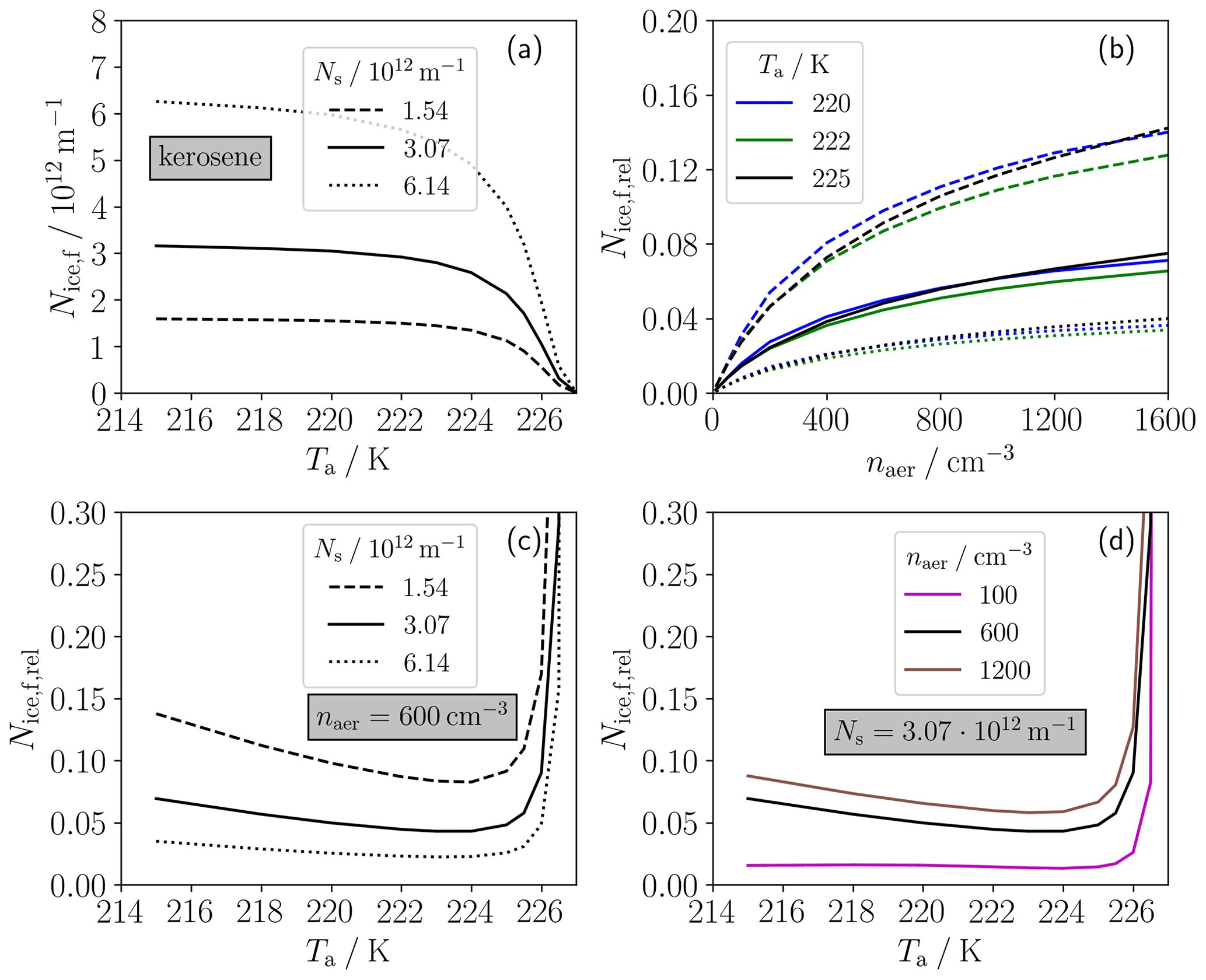
Figure 7(a) Final ice crystal number of a conventional (kerosene) contrail versus ambient temperature (Ta) for three soot particle emission numbers per flight distance Ns (different line styles). The other panels show the final ice crystal number of H2 contrails relative to the final ice crystal number of kerosene contrails in the same atmospheric conditions. Panel (b) shows versus ambient aerosol number concentration (naer) for the different soot number emissions and three Ta cases (see legend b). Panel (c) shows the temperature variation in of one H2 contrail (with naer= 600 cm−3) with respect to three kerosene contrails with different Ns values as in panel (b). Panel (d) shows the temperature variation in three H2 contrails (with different naer values as displayed in the legend) with respect to one kerosene contrail (Ns= 3.07 × 10¹² m−1). Thereby, the solid black lines in panels (c) and (d) represent the same case. The different line styles always refer to the three soot emission cases. The displayed quantities are given at a plume age of 3 s. All absolute numbers refer to a single-engine plume.
4.4.1 Mitigation potential
Figure 7 compares ice crystal numbers of conventional and H2 contrails. Panel (a) displays the ice crystal number Nice,f behind a conventional aircraft as a function of ambient temperature and for three typical soot number emission levels. For our calculated fuel consumption (that accounts for the different Q values of H2 and kerosene), the displayed soot particle numbers (Ns= 1.54 × 10¹², 3.07 × 10¹² and 6.14 × 10¹² m−1) represent soot number emission indices of around 5 × 10¹⁴, 1 × 10¹⁵ and 2 × 10¹⁵ kg−1, respectively. Prescribing our baseline ambient pressure and ambient relative humidity, the SA threshold temperature ΘG for kerosene is around 227 K (≈ 10 K lower than that for H2). Very close to ΘG, only a few soot and the entrained ambient aerosol particles can form ice crystals due to very low plume water supersaturations. For ambient temperatures (Ta⪅ΘG – 0.5 K), ice crystals mainly form on soot particles, since Ns is around 2 orders of magnitude higher than Naer during the contrail formation time (not shown). Consistently with previous studies (e.g., Kärcher et al., 2015; Bier and Burkhardt, 2019; Bier et al., 2022), Nice,f strongly increases with decreasing Ta and then approaches the respective Ns values for sufficiently low Ta. For higher Ns, the number of ice crystals formed rises more steeply and approaches Ns at lower Ta.
Now we investigate the ratio of the ice crystal numbers between H2 and kerosene contrails () shown in panels (b)–(d). We constrain our analysis to that temperature range in which kerosene contrails are able to form according to the SA criterion. Mitigation is achieved for , where a lower value is connected with a higher mitigation potential. Panel (b) shows versus naer for the three Ns values (see line style) and for three Ta cases (different colors). In general, we see a clear decrease in with increasing Ns and decreasing naer. Thereby, is below 0.1 for naer≤ 600 cm−3 and below 0.15 for higher naer. Interestingly, we see for the higher Ns and naer cases a larger difference in between 220 and 222 K than between 220 and 225 K.
Therefore, we investigate in more detail the temperature dependency of in the second row of the figure. Panel (c) shows the relative change in the ice crystal number with respect to the three soot cases for our baseline naer. In connection with the minimum at Ta ≈ 224 K, there are two different dominating effects: below 224 K, increases with decreasing Ta, in particular for the high-soot case. This is because Nice,f for the kerosene contrails approaches Ns with decreasing Ta (well below the SA threshold), while Nice,f for the H2 contrails increases further for lower Ta. The latter is because the ambient aerosol is continuously entrained into the plume and the time period for droplet and ice crystal formation increases for colder ambient conditions due to a longer-lasting water supersaturation (see Sect. 4.2). The strong increase in above around 225 K results from the strong decrease in Nice,f for the conventional contrail. This is because ice crystal formation on the weakly soluble soot particles becomes more and more limited the closer the ambient temperature approaches the SA threshold temperature. Thereby, is around 0.3 for Ta= 226.5 K and around 20 for Ta= 227 K (the latter is not visible in the figure). Finally, we show the change in ice crystal number relative to our baseline soot case but for three different naer values. The sensitivity of to naer is quite similar to that to Ns in panel (c). The most obvious difference is that an increase in naer by a factor of 2 (brown line in d) has a much lower impact on than a decrease in Ns by the same factor (dashed line in panel c). This is due to a weaker increase in the H2 contrail ice crystal number with increasing naer for high number concentrations (shown in Fig. 5a).
We can conclude that a switch to H2 combustion indicates a high mitigation potential if the ambient temperature is more than 0.5 K lower than the SA threshold temperature for kerosene. This is mainly because Naer during contrail formation is around 2 orders of magnitude lower than Ns for typical naer values. Another aspect is that the fuel consumption of a cryoplane is chosen to be around a factor of 2.8 lower than that of a corresponding conventional aircraft (only based on the difference in the combustion heat of the fuels). If air traffic with H2 combustion occurs at ambient temperatures between the kerosene SA threshold temperature and the droplet freezing temperature, clearly additional contrails are produced, which would be absent in the case of kerosene combustion.
4.4.2 Contrail visibility
We investigate the young-contrail optical thickness (τ) both for kerosene and for H2 combustion. For the quantities analyzed and presented so far, we used a reduced trajectory data set after merging trajectories with similar radial coordinates (see Sect. 3.2.1). However, the column-wise computation of τ requires spatial information of the trajectories, namely the lateral and vertical Cartesian coordinates x and z. Hence, the results presented next were obtained using the full trajectory data set from Vancassel et al. (2014). Figure 8a–d show the contrail width (indicated by the x coordinate) plume age (t) distribution of τ: the first row displays the kerosene and the second row our H2 baseline case, for Ta of both 220 K and 225 K, respectively. Observations suggest that the threshold τ for the visibility of contrails is around 0.05 (e.g., Kärcher et al., 2009). Panel (a) indicates that the kerosene contrail at Ta= 220 K becomes visible after around 0.25 s of plume age. Afterwards, the plume quickly spreads and τ tends to increase due to further formation and growth of ice crystals. Peak values of around 2 and slightly higher are reached for t between 1 and 1.5 s. For Ta= 225 K, ice crystals form later and the contrail is visible after around 0.5 s. Maximum τ is around 50 % lower than for the low-Ta case, since that contrail forms near the formation threshold and the nucleated ice crystal number is significantly reduced (see Fig. 7a, black line). For the H2 case, the optical thickness is substantially decreased compared to kerosene contrails, being consistent with the findings by Ström and Gierens (2002). Moreover, these contrails become visible later than those for kerosene at the same Ta.
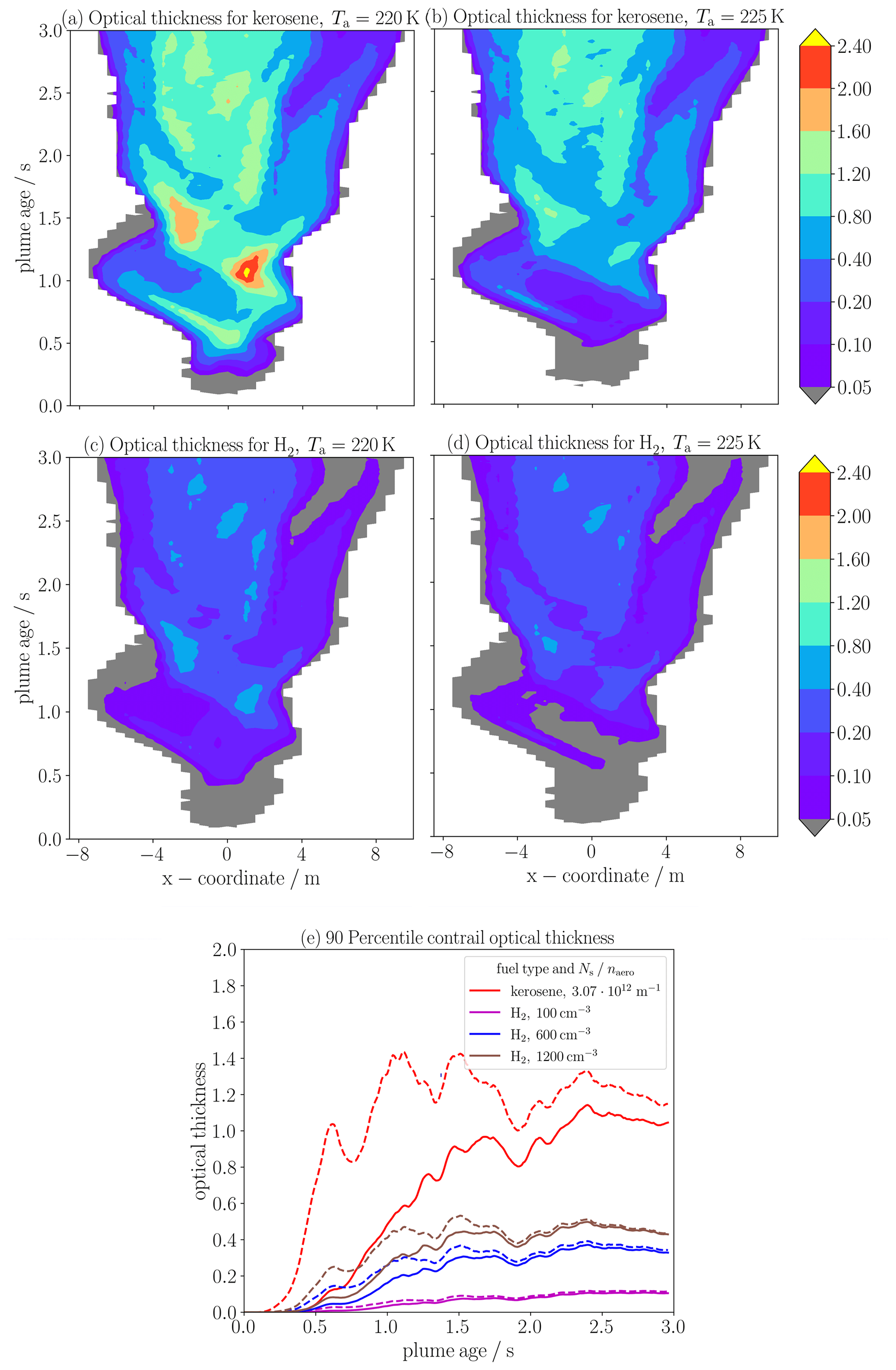
Figure 8Contour plots (a–d) of young single-engine contrail optical thickness τ over the trajectories' x coordinate indicating the contrail width and the plume age. The first row show results for kerosene (with Ns= 3.07 × 10¹² m−1) and the second for the baseline H2 case, for ambient temperature (Ta) of both 220 K on the left-hand side and 225 K on the right-hand side. Panel (e) shows the 90th-percentile optical thickness over the width τ90 for kerosene (red) and for H2 prescribing three different ambient aerosol number concentrations (other colors in the legend) for Ta= 220 K (dashed lines) and Ta= 225 K (solid lines). The temporal evolution of τ90 has been smoothed using a running-average method. For this analysis, we use the full FLUDILES trajectory ensemble of 25 000 instead of the reduced ensemble of 1000.
Finally, panel (e) shows the temporal evolution of the 90th-percentile optical thickness over the contrail width τ90. We juxtapose the kerosene contrail with three H2 contrails with different naer values. Consistent with the spatio-temporal distributions, τ90 of the H2 contrails is significantly lower than for the kerosene contrails (in particular for Ta= 220 K). The optical thickness decreases for lower naer values. We expect that the H2 contrail for naer= 100 cm−3 would be hardly visible. A lower temperature causes a slight increase in τ90 for the higher-naer cases and for t < 1.5 s. This is mainly due to the higher ice water content for lower Ta (not shown). Instead, the much stronger increase in τ for the kerosene case is due to the increased ice crystal number already at the beginning of contrail formation.
5.1 Potential sources for the formation of ultrafine volatile particles
In this study, we considered contrail ice crystals to form solely on ambient particles entrained in the plume. While H2 combustion emissions are in general expected to be soot-free, the formation of ultrafine volatile particles (UFPs), which can also contribute to contrail ice crystal formation, is still possible. Two potential sources for the formation of UFPs behind H2 combustion engines are discussed in the following.
5.1.1 Nitrogen compounds
Several recent studies have considered chemi-ions that are mainly composed of sulfur species (e.g., Yu and Turco, 1997). While sulfur is likely not produced during H2 combustion, NOx is still emitted. The reaction of NOx with H2O and OH species potentially leads to the formation of nitrogen compounds like nitric acid that have been observed in conventional aircraft plumes (e.g., Tremmel et al., 1998). Moreover, Wang et al. (2020) have shown within cloud chamber experiments that nitric acid and ammonia can nucleate directly to form volatile ammonium nitrate particles at temperatures below 258 K. Finally, nitrogen species might be a potential source of the nucleation of ultrafine volatile particles in both conventional and H2 combustion plumes, but the formation process behind this is not yet sufficiently understood.
5.1.2 Ultrafine oil particles
We expect that engine lubrication systems will continue to be used for H2 engines, causing emissions of oil vapors. Even though an air–oil separator recovers around 99 % of the oil emissions, the residual may contaminate the engine plume. Ungeheuer et al. (2022) have shown in laboratory experiments that “jet oil vapors reach gas-phase supersaturation in cooling emission plumes leading to rapid nucleation and formation of ultrafine volatile particles in the range of ∼ 10–20 nm.” These diameter ranges appear to be consistent with the ground-measured ambient UFPs downwind of Frankfurt Airport, in which organic engine oil constituents have been identified (Ungeheuer et al., 2021).
The UFPs formed can contribute to droplet and ice crystal formation in addition to the background aerosol. Assuming a typical oil consumption of around 1 L h−1 with 1 % volume fraction (residual) that enters the plume, our estimates suggest that the UFP number per flight distance could be even larger than that of soot particles. Since plume water supersaturations are much higher for H2 than for kerosene in the same ambient conditions, we expect that droplets and ice crystals would mainly form on those UFPs rather than on the entrained ambient particles. This means that the number of ice crystals could be similar or even increased compared to conventional contrails. One should still keep in mind that the experiments of Ungeheuer et al. (2022) refer to conventional kerosene combustion and that the properties of the oil particles (size and chemical composition) could significantly change for H2. Moreover, associate measurements in cruise altitude conditions are necessary to confirm the occurrence of those UFPs.
Finally, a hermetic and clean sealing of the engines from the oil system aimed at a complete jet oil recovery could be a technical means to achieve a valuable mitigation effort for contrail formation if future model studies and flight campaigns give indications of abundant droplet formation on oil particles.
5.2 Scaling relations for different plume area evolution and fuel consumption levels
In the present study, we use the FLUDILES trajectory data (Vancassel et al., 2014) that were modified according to the description in Sect. 3.2.1. The presented results represent a single-engine plume of an A340 aircraft. Extensive contrail quantities (like ice crystal number and mass) for the whole aircraft may be scaled with the number of engines (in our case, it is four). This scaling is valid as long as we assume that there is no interference from the two exhaust plumes (on one side of the aircraft) during the contrail formation stage. This scaling could also be interpreted as a scaling with the ratio of the total fuel consumption (mC,tot) and our reference value mC= 1.1 g m−1 (for the baseline Ta and pa values). Basically, one could plug in any reasonable value for mC,tot. However, this flexible fuel consumption scaling approach is only valid with several underlying assumptions that are usually not fulfilled. Firstly, one has to assume that the initial plume area AE scales with the fuel consumption and, secondly, that the plume dilution 𝒞(t) is independent of AE and hence A(t)∼AE.
However, Lewellen (2020) showed that the evolution of 𝒞 itself depends on engine size. Different dilution impacts not only the plume area evolution but also the thermodynamic plume and the microphysical contrail properties (Lewellen, 2020; Bier et al., 2022). Neglecting those constraints and assuming fixed atmospheric conditions and aerosol particle properties, we observe that . This behavior is similar to that of kerosene contrails, where we find . Again, this is only a rough estimate with several underlying assumptions and for a fixed soot number emission index of EI.
So far, we have stressed that the given reference value of mC holds (only) for the baseline values of ambient temperature and pressure. In our study, we use a constant AE, which refers to a particular aircraft type with an engine nozzle radius of 0.5 m (see Table 2). Moreover, we keep the plume exit temperature TE fixed in our setup.
From Eqs. (4) and (10), it follows that the initial dilution and, correspondingly, the fuel consumption implicitly change when Ta takes a different value (. However, this Ta dependence of CE and mC is much less crucial for Nice than the impact of Ta on the plume relative humidity evolution. A change in ambient pressure pa does not affect 𝒞E, but mC changes linearly with pa. Hence, the implied mC values in our pa sensitivity study differ non-negligibly. Clearly, these changes in the mC values are consequences of our choices in the study design. In reality, the fuel consumption depends on the thrust setting and may change differently to how we prescribed it when pa and/or Ta change (see, e.g., Lewellen, 2020; Volponi, 1998; Kurzke, 2003).
5.3 Deliquescence relative humidity
We prescribe a fixed deliquescence relative humidity of the aerosol particles, DRH =0.99 in our setup, a value close to water saturation. The definition of a lower baseline value (according to Peng et al., 2022) with appropriate sensitivity variations would have been more reasonable. However, in several test simulations we did not achieve robust results for DRH ⪅0.95, in particular for the low mean aerosol particle dry size and hygroscopicity parameter. This is likely due to one technical aspect: while water saturation is reached first near the plume edge and later on in the plume center in the first tenths of a second, higher relative humidities last longer in the plume center than at the edge towards the end of contrail formation (see, e.g., Fig. 1d of Bier et al., 2022). The lower the DRH value, the longer the potential time period for droplet and subsequent ice crystal formation, in particular for lower ambient temperatures. The ambient particles are mainly entrained near the plume edge. Since we cannot resolve this heterogeneous entrainment but ambient particles are mixed in for each trajectory with equal share, droplet and ice crystal formation is likely overestimated, and this overestimation increases with decreasing DRH.
In the recent past, several model studies have investigated contrail formation behind commercial aircraft by means of analytical approaches (Kärcher et al., 2015; Bier and Burkhardt, 2019), 0D box models (e.g., Kärcher and Yu, 2009; Vancassel et al., 2014; Bier et al., 2022) and LES (e.g., Paoli et al., 2013; Khou et al., 2015; Lewellen, 2020). These studies focused on contrail formation on soot particles on which the majority of ice crystals form for conventional engines (e.g., Kärcher and Yu, 2009; Kleine et al., 2018). Switching to liquid hydrogen (H2) propulsion, ice crystals are expected to form solely on background particles mixed into the plume. Even though some of those studies account for ice crystal formation on background particles (e.g., Kärcher and Yu, 2009; Kärcher et al., 2015; Lewellen, 2020), the implementation of this process has been somewhat simplified (e.g., activation relaxation approach in Kärcher et al., 2015) and ambient particle properties are mostly kept fixed.
While Bier et al. (2022) have extended the particle-based Lagrangian Cloud Module (LCM; Sölch and Kärcher, 2010) by contrail formation microphysics on soot particles, we here advance the LCM by specific contrail formation microphysics on entrained background aerosol particles. The most relevant feature is that ambient particles are continuously entrained into the plume instead of releasing a fixed number of soot particles. Moreover, we define an alternative droplet activation criterion and improve the homogeneous freezing parameterization by accounting for the impact of the solution effect on droplet freezing.
Given the same atmospheric conditions and propulsion efficiency, the Schmidt–Appleman (SA) threshold temperature (Schumann, 1996) is around 10 K higher for H2 than for kerosene-fueled aircraft due to water vapor emissions that are around 2.6 times higher for the same amount of released combustion heat. The homogeneous freezing temperature of water droplets is in general lower than the SA threshold temperature for H2 contrails and, therefore, becomes a more limiting criterion for contrail formation, as already pointed out by Gierens (2021).
The ice crystal number is strongly cut down for temperatures above around 230 K since smaller droplets no longer freeze into ice crystals. Contrails cannot form anymore at temperatures above around 233–234 K in our study. While for kerosene combustion the number of ice crystals formed approaches the emitted soot particle number for a sufficiently low ambient temperature (e.g., Kärcher et al., 2015), the ice crystal number of H2 contrails increases further with decreasing temperature. The latter is because the water supersaturation in the plume lasts longer for colder conditions, and, hence, more of the entrained aerosol particles can form droplets and ice crystals.
Our results highlight a large variability in the number of contrail ice crystals formed with varying ambient aerosol properties. For a fixed particle size distribution and chemical composition, the ice crystal number clearly rises with increasing aerosol number concentration. This increase becomes weaker for higher number concentrations (⪆ 200 cm−3), in particular in a colder environment. The variation in contrail ice nucleation with aerosol mean dry size and water solubility is low for larger aerosol particles and high for small (mean radius ⪅ 10 nm) particles. For these smaller particles, the sensitivity of the ice crystal number to the water solubility of the aerosol particles is quite complex for lower temperatures due to various counteracting microphysical processes.
In the real atmosphere, the background aerosol typically consists of multiple particle types with different mean dry sizes (modes) and chemical composition. Therefore, we analyze contrail formation prescribing two co-existing aerosol particle ensembles that differ in either the mean dry size or hygroscopicity parameter. If these co-existing particle ensembles contain only larger (mean dry radii more than around 10 nm) and well-soluble aerosol particles, the ice crystal number for each of the ensembles can be estimated well from a simulation with appropriate single particle ensembles. The total ice crystal number of the co-existing particle ensembles can also be approximated from one single particle ensemble prescribing average properties of mean dry size and solubility and the total number concentration of the co-existing particle ensembles. This is because the ice crystal number is not as sensitive to changes in this large particle range, as mentioned above. Conversely, such an approach is not meaningful if a substantial fraction of small and weakly soluble aerosol particles (in particular nucleation-mode particles) are present. If these particles co-exist with larger and/or more soluble particles, droplet and ice crystal formation on these particles might be significantly suppressed due to the competition effects between the aerosol particles. Due to the non-linearity between ice crystal number and mean dry size for small particles, the total ice crystal number of the co-existing particle ensembles might be significantly different to the average single particle ensemble.
Finally, we compare ice crystal formation, as a first measure of mitigation potential, and visibility of H2 contrails with conventional contrails. Varying both the aerosol number concentration and soot number emissions, the H2 contrail ice crystal number is significantly reduced (by more than 80 %–90 %) compared to conventional contrails, implying a great mitigation potential. This is mainly because ambient aerosol number concentrations are at least 1-2 orders of magnitude lower than soot particle number concentrations in young exhaust plumes behind conventional aircraft. For ambient temperatures only slightly below (⪅ 0.5 K) the SA threshold temperature for kerosene combustion, the H2 contrail ice crystal number can be higher, since ice crystal formation on the weakly soluble soot particles becomes strongly limited by very low plume water supersaturations (e.g., Kärcher et al., 2015). The optical thickness is significantly decreased, and the H2 contrails either become visible slightly later or might not be visible at all for low ambient aerosol number concentrations. On the other hand, H2 contrails can form at lower flight altitudes (connected with ambient temperatures lying between the SA threshold temperature for kerosene and the homogeneous freezing temperature of the water droplets) than conventional contrails, as also mentioned by Ström and Gierens (2002). In the case of persistent contrails, this would increase the contrail coverage and counteract the climate benefits of low-ice-number contrails.
Once RHwat surpasses DRH for the first time, a new SIP ensemble that represents the newly entrained dry aerosol is created at every time step. In order to keep the total SIP number in an acceptable range, we employ a SIP merging technique whereby several similarly sized SIPs of the same category (aerosol, droplets and ice crystals) are merged into a single SIP. The merge operation is implemented such that the number and mass of the represented physical particles are conserved (Unterstrasser and Sölch, 2014). The SIP merging is executed when NSIP exceeds a certain threshold value (fixed to 1600 in our study). Then the new NSIP value is well below that threshold and starts to increase again. In the end, the SIP number follows a jigsaw pattern as exemplarily shown in Fig. A1. The merge operation has some more (internal) parameters, e.g., how many SIPs are at most merged and what is the maximum relative difference between SIPs that are merged. We experimented with those parameters and found numerical convergence, which means our present configuration yields basically identical results to simulations with higher NSIP values.
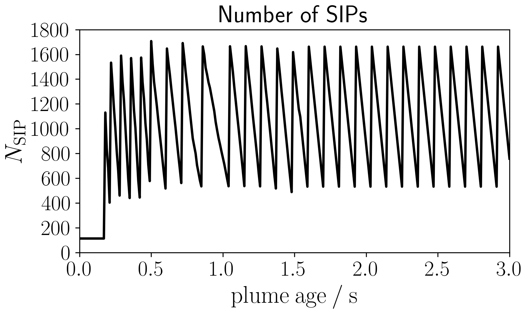
We calculate the homogeneous freezing temperature as
where Tfrz,0 is the freezing temperature assuming a pure supercooled water droplet (awat=1). It is determined from Eq. (6) of Bier et al. (2022) following the approach of Kärcher et al. (2015) and Riechers et al. (2013) and varies with droplet water volume Vwat and cooling rate .
The second term is a correction term based on the study from O and Wood (2016) approximating the decrease in Tfrz with decreasing activity of water awat (e.g., Koop et al., 2000). O and Wood (2016) developed an approximation for the homogeneous freezing temperature of solution droplets (Tfrz,owood) as a function of water volume and activity but neglected the cooling rate. Thereby, that temperature for which the mean number of critical embryos becomes equal to 1 is iteratively calculated, triggering the freezing process in the droplet (see their Eq. 1). For our activated water droplets (awat > 0.90), we find that the parameterization yields robust results for droplet radii r≥1 µm. On the other hand, the solution effect is frequently important for smaller droplets (r < 1 µm) formed on freshly entrained aerosol particles.
For simplicity, we prescribe a fixed droplet radius r=1 µm for the estimation of our correction term. We evaluate Tfrz,owood for different awat values that result from a variation in rd. Setting and , we define the following quadratic fit function,
which is valid for awat≥0.90 with the fit parameters a=345.746, b=100.977 and c=0.01687 and a square root mean error R2=0.99999. Even though the expression for ΔT is a simplified correction term, Eq. (B1) combines the sensitivity of the homogeneous freezing to all major effects.
Figure B1 shows the variation in Tfrz with droplet radius r and water activity for a plume cooling rate of −10 K s−1. For awat= 1 (representing pure water droplets), Tfrz equals Tfrz,0 and ranges between around 229 and 233 K. Thereby, Tfrz increases with rising r. The strong decrease in Tfrz with decreasing awat (for fixed r) down to around 215 K emphasizes the importance of accounting for the solution effect in droplets. In contrast, the impact of a varying cooling rate is low (not shown).
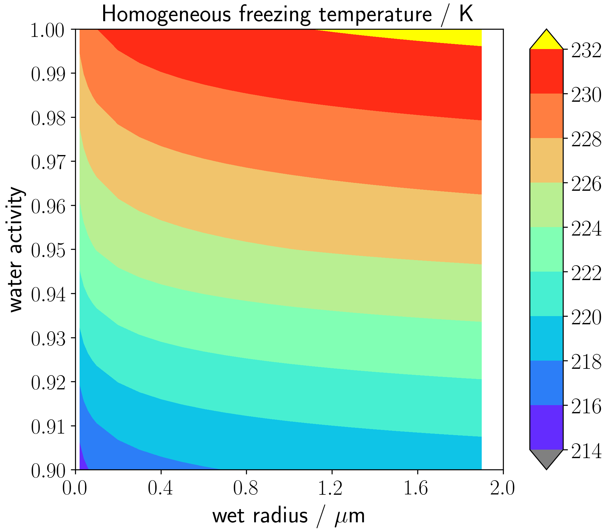
Figure B1Contour plot showing the homogeneous freezing temperature of supercooled solution droplets over the wet radius and water activity. The cooling rate is set to −10 K s−1.
The presented data are available from the corresponding author upon request (andreas.bier@dlr.de).
AB performed the simulations, created the tables and figures, and wrote the first draft of the manuscript. AB and SU conceptualized the study, and they evaluated and interpreted the results. AB, SU, JZ and TJW wrote and edited the manuscript. AB, SU, JZ, DH and AL advanced and extended the box model code. JZ updated the figures during the revision.
The contact author has declared that none of the authors has any competing interests.
Publisher’s note: Copernicus Publications remains neutral with regard to jurisdictional claims made in the text, published maps, institutional affiliations, or any other geographical representation in this paper. While Copernicus Publications makes every effort to include appropriate place names, the final responsibility lies with the authors.
This work has been funded by the DLR internal project “H2CONTRAIL”. We thank Xavier Vancassel for providing the original FLUDILES trajectory data set.
This research has been supported by the Deutsche Forschungsgemeinschaft (DFG; grant no. BI 2128/1-1) and the HORIZON-JU-Clean-Aviation project HYDEA (grant agreement ID 101102019; https://doi.org/10.3030/101102019).
This paper was edited by Farahnaz Khosrawi and reviewed by two anonymous referees.
Airbus: How Blue Condor will accelerate Airbus' first hydrogen-powered test flights, https://www.airbus.com/en/newsroom/stories/2022-07-how-blue-condor-will-accelerate-airbus-first-hydrogen-powered-test-flights (last access: 19 February 2024), 2022. a
Andreae, M. O., Jones, C. D., and Cox, P. M.: Strong present-day aerosol cooling implies a hot future, Nature, 435, 1187–1190, https://doi.org/10.1038/nature03671, 2005. a
Beer, C. G., Hendricks, J., Righi, M., Heinold, B., Tegen, I., Groß, S., Sauer, D., Walser, A., and Weinzierl, B.: Modelling mineral dust emissions and atmospheric dispersion with MADE3 in EMAC v2.54, Geosci. Model Dev., 13, 4287–4303, https://doi.org/10.5194/gmd-13-4287-2020, 2020. a, b
Beer, C. G., Hendricks, J., and Righi, M.: A global climatology of ice-nucleating particles under cirrus conditions derived from model simulations with MADE3 in EMAC, Atmos. Chem. Phys., 22, 15887–15907, https://doi.org/10.5194/acp-22-15887-2022, 2022. a
Bier, A. and Burkhardt, U.: Variability in Contrail Ice Nucleation and Its Dependence on Soot Number Emissions, J. Geophys. Res., 124, 3384–3400, https://doi.org/10.1029/2018JD029155, 2019. a, b, c, d
Bier, A. and Burkhardt, U.: Impact of parametrizing microphysical processes in the jet and vortex phase on contrail cirrus properties and radiative forcing, J. Geophys. Res., 127, e2022JD036677, https://doi.org/10.1029/2022JD036677, 2022. a, b, c, d
Bier, A., Burkhardt, U., and Bock, L.: Synoptic Control of Contrail Cirrus Life Cycles and Their Modification Due to Reduced Soot Number Emissions, J. Geophys. Res., 122, 11584–11603, https://doi.org/10.1002/2017JD027011, 2017. a, b
Bier, A., Unterstrasser, S., and Vancassel, X.: Box model trajectory studies of contrail formation using a particle-based cloud microphysics scheme, Atmos. Chem. Phys., 22, 823–845, https://doi.org/10.5194/acp-22-823-2022, 2022. a, b, c, d, e, f, g, h, i, j, k, l, m, n, o, p, q, r, s, t, u, v, w, x, y, z, aa, ab, ac, ad, ae
Bock, L. and Burkhardt, U.: The temporal evolution of a long-lived contrail cirrus cluster: Simulations with a global climate model, J. Geophys. Res., 121, 3548–3565, https://doi.org/10.1002/2015JD024475, 2016a. a
Bock, L. and Burkhardt, U.: Reassessing properties and radiative forcing of contrail cirrus using a climate model, J. Geophys. Res., 121, 9717–9736, https://doi.org/10.1002/2016JD025112, 2016b. a
Borrmann, S., Kunkel, D., Weigel, R., Minikin, A., Deshler, T., Wilson, J. C., Curtius, J., Volk, C. M., Homan, C. D., Ulanovsky, A., Ravegnani, F., Viciani, S., Shur, G. N., Belyaev, G. V., Law, K. S., and Cairo, F.: Aerosols in the tropical and subtropical UT/LS: in-situ measurements of submicron particle abundance and volatility, Atmos. Chem. Phys., 10, 5573–5592, https://doi.org/10.5194/acp-10-5573-2010, 2010. a, b
Boucher, O., Randall, D., Artaxo, P., Bretherton, C., Feingold, G., Forster, P., Kerminen, V.-M., Kondo, Y., Liao, H., Lohmann, U., Rasch, P., Satheesh, S., Sherwood, S., Stevens, B., and Zhang, X.: Clouds and Aerosols, Chap. 7, Cambridge University Press, Cambridge, United Kingdom and New York, NY, USA, 571–658, https://doi.org/10.1017/CBO9781107415324.016, ISBN 978-1-107-66182-0, 2013. a
Brock, C. A., Froyd, K. D., Dollner, M., Williamson, C. J., Schill, G., Murphy, D. M., Wagner, N. J., Kupc, A., Jimenez, J. L., Campuzano-Jost, P., Nault, B. A., Schroder, J. C., Day, D. A., Price, D. J., Weinzierl, B., Schwarz, J. P., Katich, J. M., Wang, S., Zeng, L., Weber, R., Dibb, J., Scheuer, E., Diskin, G. S., DiGangi, J. P., Bui, T., Dean-Day, J. M., Thompson, C. R., Peischl, J., Ryerson, T. B., Bourgeois, I., Daube, B. C., Commane, R., and Wofsy, S. C.: Ambient aerosol properties in the remote atmosphere from global-scale in situ measurements, Atmos. Chem. Phys., 21, 15023–15063, https://doi.org/10.5194/acp-21-15023-2021, 2021. a, b, c, d
Bräuer, T., Voigt, C., Sauer, D., Kaufmann, S., Hahn, V., Scheibe, M., Schlager, H., Huber, F., Le Clercq, P., Moore, R. H., and Anderson, B. E.: Reduced ice number concentrations in contrails from low-aromatic biofuel blends, Atmos. Chem. Phys., 21, 16817–16826, https://doi.org/10.5194/acp-21-16817-2021, 2021. a, b
Burkhardt, U., Bock, L., and Bier, A.: Mitigating the contrail cirrus climate impact by reducing aircraft soot number emissions, npj Climate and Atmospheric Science, 1, 37, https://doi.org/10.1038/s41612-018-0046-4, 2018. a, b, c
Busen, R. and Schumann, U.: Visible contrail formation from fuels with different sulfur contents, Geophys. Res. Lett., 22, 1357–1360, 1995. a
Froyd, K. D., Murphy, D. M., Brock, C. A., Campuzano-Jost, P., Dibb, J. E., Jimenez, J.-L., Kupc, A., Middlebrook, A. M., Schill, G. P., Thornhill, K. L., Williamson, C. J., Wilson, J. C., and Ziemba, L. D.: A new method to quantify mineral dust and other aerosol species from aircraft platforms using single-particle mass spectrometry, Atmos. Meas. Tech., 12, 6209–6239, https://doi.org/10.5194/amt-12-6209-2019, 2019. a
Fuchs, N. and Sutugin, A. G.: Highly dispersed aerosols, Topics in Current Aerosol Research, 2, 1–60, 1971. a
Gierens, K.: Theory of Contrail Formation for Fuel Cells, Aerospace, 8, 164, https://doi.org/10.3390/aerospace8060164, 2021. a
Hacker, P. T.: Experimental Values of the Surface Tension of Supercooled Water, Tech. rep., Technical Note 2510, National Advisory, https://ntrs.nasa.gov/api/citations/19810068863/downloads/19810068863.pdf (last access: 19 February 2024), 1951. a
Hendricks, J., Kärcher, B., and Lohmann, U.: Effects of ice nuclei on cirrus clouds in a global climate model, J. Geophys. Res., 116, D18206, https://doi.org/10.1029/2010JD015302, 2011. a
Hermann, J., Heintzenberg, J., Wiedensohler, A., Zahn, A., Heinrich, G., and Brenninkmeijer, C. A. M.: Meridional distributions of aerosol particle number concentrations in the upper troposphere and lower stratosphere obtained by Civil Aircraft for Regular Investigation of the Atmosphere Based on an Instrument Container (CARIBIC) flights, J. Geophys. Res., 108, 4114, https://doi.org/10.1029/2001JD001077, 2003. a, b, c
Kaiser, J. C., Hendricks, J., Righi, M., Jöckel, P., Tost, H., Kandler, K., Weinzierl, B., Sauer, D., Heimerl, K., Schwarz, J. P., Perring, A. E., and Popp, T.: Global aerosol modeling with MADE3 (v3.0) in EMAC (based on v2.53): model description and evaluation, Geosci. Model Dev., 12, 541–579, https://doi.org/10.5194/gmd-12-541-2019, 2019. a
Kärcher, B.: Formation and radiative forcing of contrail cirrus, Nat. Commun., 9, 1824, https://doi.org/10.1038/s41467-018-04068-0, 2018. a
Kärcher, B. and Yu, F.: Role of aircraft soot emissions in contrail formation, Geophys. Res. Lett., 36, L01804, https://doi.org/10.1029/2008GL036649, 2009. a, b, c, d, e, f
Kärcher, B., Peter, T., Biermann, U., and Schumann, U.: The Initial Composition of Jet Condensation Trails, J. Atmos. Sci., 53, 3066–3083, 1996. a, b
Kärcher, B., Burkhardt, U., Unterstrasser, S., and Minnis, P.: Factors controlling contrail cirrus optical depth, Atmos. Chem. Phys., 9, 6229–6254, https://doi.org/10.5194/acp-9-6229-2009, 2009. a
Kärcher, B., Burkhardt, U., Bier, A., Bock, L., and Ford, I. J.: The microphysical pathway to contrail formation, J. Geophys. Res., 120, 7893–7927, https://doi.org/10.1002/2015JD023491, 2015JD023491, 2015. a, b, c, d, e, f, g, h, i, j, k, l, m, n, o, p
Khou, J.-C., Ghedhaïfi, W., Vancassel, X., and Garnier, F.: Spatial Simulation of Contrail Formation in Near-Field of Commercial Aircraft, J. Aircraft, 52, 1927–1938, https://doi.org/10.2514/1.C033101, 2015. a
Kleine, J., Voigt, C., Sauer, D., Schlager, H., Scheibe, M., Jurkat-Witschas, Kaufmann, S., Kärcher, B., and Anderson, B. E.: In situ observations of ice particle losses in a young persistent contrail, Geophys. Res. Lett., 45, 13553–13561, https://doi.org/10.1029/2018GL079390, 2018. a, b
Koop, T., Luo, B., Tsias, A., and Peter, T.: Water activity as the determinant for homogeneous ice nucleation in aqueous solutions, Nature, 406, 611–4, 2000. a, b
Kulmala, M.: Condensational Growth and Evaporation in the Transition Regime, Aerosol Sci. Technol., 19, 381–388, https://doi.org/10.1080/02786829308959645, 1993. a
Kumar, P., Sokolik, I. N., and Nenes, A.: Parameterization of cloud droplet formation for global and regional models: including adsorption activation from insoluble CCN, Atmos. Chem. Phys., 9, 2517–2532, https://doi.org/10.5194/acp-9-2517-2009, 2009. a
Kurzke, J.: Model based gas turbine parameter corrections, in: Vol. 1, ASME Turbo Expo 2003, collocated with the 2003 International Joint Power Generation Conference, 16–19 June 2003 Atlanta, Georgia, USA, 91–99, https://doi.org/10.1115/GT2003-38234, 2003. a
Lee, D. S., Fahey, D. W., Skowron, A., Allen, M. R., Burkhardt, U., Chen, Q., Doherty, S. J., Freemann, S., Forster, P. M., Fuglestvedt, J., Gettelman, A., De Leon, R. R., Lim, L. L., Lund, T. M., Miller, R. J., Owen, B., Penner, J. E., Pitari, G., Prather, M. J., Sausen, R., and Wilcox, L. J.: The contribution of global aviation to anthropogenic climate forcing for 2010 to 2018, Atmos. Environ., 244, 117834, https://doi.org/10.1016/j.atmosenv.2020.117834, 2021. a
Lee, S.-H., Reeves, J. M., Wilson, J. C., Hunton, D. E., Viggiano, A. A., Miller, T. M., Ballenthin, J. O., and Lait, L. R.: Particle Formation by Ion Nucleation in the Upper Troposphere and Lower Stratosphere, Science, 301, 1886–1889, https://doi.org/10.1126/science.1087236, 2003. a
Lewellen, D. C.: A Large-Eddy Simulation Study of Contrail Ice Number Formation, J. Atmos. Sci., 77, 2585–2604, https://doi.org/10.1175/JAS-D-19-0322.1, 2020. a, b, c, d, e, f
Liu, H. J., Zhao, C. S., Nekat, B., Ma, N., Wiedensohler, A., van Pinxteren, D., Spindler, G., Müller, K., and Herrmann, H.: Aerosol hygroscopicity derived from size-segregated chemical composition and its parameterization in the North China Plain, Atmos. Chem. Phys., 14, 2525–2539, https://doi.org/10.5194/acp-14-2525-2014, 2014. a, b
Marcolli, C.: Pre-activation of aerosol particles by ice preserved in pores, Atmos. Chem. Phys., 17, 1595–1622, https://doi.org/10.5194/acp-17-1595-2017, 2017. a
Marquart, S., Ponater, M., Ström, L., and Gierens, K.: An upgraded estimate of the radiative forcing of cryoplane contrails, Meteorol. Z., 14, 573–582, 2005. a
Mason, B.: The physics of clouds, Clarendon Press, Oxford, ISBN 10 0198516037, https://openlibrary.org/books/OL5692210M/The_physics_of_clouds (last access: 19 February 2024), 1971. a
Minikin, A., Petzold, A., Ström, J., Krejci, R., Seifert, M., van Velthoven, P., Schlager, H., and Schumann, U.: Aircraft observations of the upper tropospheric fine particle aerosol in the Northern and Southern Hemispheres at midlatitudes, Geophys. Res. Lett., 30, 1503, https://doi.org/10.1029/2002GL016458, 2003. a, b, c, d
Moore, R. H., Thornhill, K. L., Weinzierl, B., Sauer, D., D'Ascoli, E., Kim, J., Lichtenstern, M., Scheibe, M., Beaton, B., Beyersdorf, A. J., Barrick, J., Bulzan, D., Corr, C. A., Crosbie, E., Jurkat, T., Martin, R., Riddick, D., Shook, M., Slover, G., Voigt, C., White, R., Winstead, E., Yasky, R., Ziemba, L. D., Brown, A., Schlager, H., and Anderson, B. E.: Biofuel blending reduces particle emissions from aircraft engines at cruise conditions, Nature, 543, 411–415, https://doi.org/10.1038/nature21420, 2017. a
Najjar, Y.: Hydrogen safety: The road toward green technology., Int. J. Hydrogen Energ., 38, 10716–10728, https://doi.org/10.1016/j.ijhydene.2013.05.126, 2013. a
O, K.-T. and Wood, R.: Exploring an approximation for the homogeneous freezing temperature of water droplets, Atmos. Chem. Phys., 16, 7239–7249, https://doi.org/10.5194/acp-16-7239-2016, 2016. a, b, c
Padro, L. T., Tkacik, D., Lathem, T., Hennigan, C. J., Sullivan, A. P., Weber, R. J., Huey, L. G., and Nenes, A.: Investigation of cloud condensation nuclei properties and droplet growth kinetics of the water-soluble aerosol fraction in Mexico City, J. Geophys. Res., 115, D09204, https://doi.org/10.1029/2009JD013195, 2010. a
Paoli, R., Nybelen, L., Picot, J., and Cariolle, D.: Effects of jet/vortex interaction on contrail formation in supersaturated conditions, Phys. Fluids, 25, 1–28, https://doi.org/10.1063/1.4807063, 2013. a
Peng, C., Chen, L., and Tang, M.: A database for deliquescence and efflorescence relative humidities of compounds with atmospheric relevance, Fundamental Research, 2, 578–587, 2022. a, b
Petters, M. D. and Kreidenweis, S. M.: A single parameter representation of hygroscopic growth and cloud condensation nucleus activity, Atmos. Chem. Phys., 7, 1961–1971, https://doi.org/10.5194/acp-7-1961-2007, 2007. a, b, c
Petzold, A., Fiebig, M., Keil, A., Leiterer, U., Schröder, F., Stifter, A., Wendisch, M., and Wendling, P.: Vertical variability of aerosol properties observed at a continental site during the Lindenberg Aerosol Characterization Experiment (LACE 98), J. Geophys. Res., 107, 8128, https://doi.org/10.1029/2001JD001043, 2002. a
Petzold, A., Gysel, M., Vancassel, X., Hitzenberger, R., Puxbaum, H., Vrochticky, S., Weingartner, E., Baltensperger, U., and Mirabel, P.: On the effects of organic matter and sulphur-containing compounds on the CCN activation of combustion particles, Atmos. Chem. Phys., 5, 3187–3203, https://doi.org/10.5194/acp-5-3187-2005, 2005. a
Pletzer, J., Hauglustaine, D., Cohen, Y., Jöckel, P., and Grewe, V.: The climate impact of hydrogen-powered hypersonic transport, Atmos. Chem. Phys., 22, 14323–14354, https://doi.org/10.5194/acp-22-14323-2022, 2022. a
Ponater, M., Marquart, S., and Sausen, R.: Contrails in a comprehensive global climate model: Parameterization and radiative forcing results, J. Geophys. Res., 107, 941–960, 2002. a
Ponater, M., Pechtl, S., Sausen, R., Schumann, U., and Hüttig, G.: Potential of the cryoplane technology to reduce aircraft climate impact: A state-of-the-art assessment, Atmos. Environ., 40, 6928–6944, 2006. a
Riechers, B., Wittbracht, F., Hütten, A., and Koop, T.: The homogeneous ice nucleation rate of water droplets produced in a microfluidic device and the role of temperature uncertainty, Phys. Chem. Chem. Phys., 15, 5873–5887, https://doi.org/10.1039/c3cp42437e, 2013. a, b
Righi, M., Hendricks, J., and Sausen, R.: The global impact of the transport sectors on atmospheric aerosol: simulations for year 2000 emissions, Atmos. Chem. Phys., 13, 9939–9970, https://doi.org/10.5194/acp-13-9939-2013, 2013. a
Righi, M., Hendricks, J., and Sausen, R.: The global impact of the transport sectors on atmospheric aerosol in 2030 – Part 2: Aviation, Atmos. Chem. Phys., 16, 4481–4495, https://doi.org/10.5194/acp-16-4481-2016, 2016. a
Rogers, D. C., DeMott, P. J., Kreidenweis, S. M., and Chen, Y.: Measurements of ice nucleating aerosols during SUCCESS, Geophys. Res. Lett., 25, 1383–1386, https://doi.org/10.1029/97gl03478, 1998. a
Schmale, J., Schneider, J., Jurkat, T., Voigt, C., Kalesse, H., Rautenhaus, M., Lichtenstern, M., Schlager, H., Ancellet, G., Arnold, F., Gerding, M., Mattis, I., Wendisch, M., and Borrmann, S.: Aerosol layers from the 2008 eruptions of Mount Okmok and Mount Kasatochi: In situ upper troposphere and lower stratosphere measurements of sulfate and organics over Europe, J. Geophys. Res., 115, D00L07, https://doi.org/10.1029/2009JD013628, 2010. a
Schumann, U.: On conditions for contrail formation from aircraft exhausts, Meteorol. Z., 5, 4–23, 1996. a, b, c, d, e, f, g
Schumann, U., Arnold, F., Busen, R., Curtius, J., Kärcher, B., Kiendler, A., Petzold, A., Schlager, H., Schröder, F., and Wohlfrom, K.: Influence of fuel sulfur on the composition of aircraft exhaust plumes: The experiments SULFUR 1-7, J. Geophys. Res., 107, 4247, https://doi.org/10.1029/2001JD000813, 2002. a
Sölch, I. and Kärcher, B.: A large-eddy model for cirrus clouds with explicit aerosol and ice microphysics and Lagrangian ice particle tracking, Q. J. Roy. Meteor. Soc., 136, 2074–2093, https://doi.org/10.1002/qj.689, 2010. a, b
Sölch, I. and Kärcher, B.: Process-oriented large-eddy simulations of a midlatitude cirrus cloud system based on observations, Q. J. Roy. Meteor. Soc., 137, 374–393, 2011. a
Sorjamaa, R. and Laaksonen, A.: The effect of H2O adsorption on cloud drop activation of insoluble particles: a theoretical framework, Atmos. Chem. Phys., 7, 6175–6180, https://doi.org/10.5194/acp-7-6175-2007, 2007. a
Stier, P., Feichter, J., Kinne, S., Kloster, S., Vignati, E., Wilson, J., Ganzeveld, L., Tegen, I., Werner, M., Balkanski, Y., Schulz, M., Boucher, O., Minikin, A., and Petzold, A.: The aerosol-climate model ECHAM5-HAM, Atmos. Chem. Phys., 5, 1125–1156, https://doi.org/10.5194/acp-5-1125-2005, 2005. a
Ström, L. and Gierens, K.: First simulations of cryoplane contrails, J. Geophys. Res., 107, 4346, https://doi.org/10.1029/2001JD000838, 2002. a, b, c, d
Tomsche, L., Marsing, A., Jurkat-Witschas, T., Lucke, J., Kaufmann, S., Kaiser, K., Schneider, J., Scheibe, M., Schlager, H., Röder, L., Fischer, H., Obersteiner, F., Zahn, A., Zöger, M., Lelieveld, J., and Voigt, C.: Enhanced sulfur in the upper troposphere and lower stratosphere in spring 2020, Atmos. Chem. Phys., 22, 15135–15151, https://doi.org/10.5194/acp-22-15135-2022, 2022. a
Tremmel, H. G., Schlager, H., Konopka, P., Schulte, P., Arnold, F., Klemm, M., and Droste-Franke, B.: Observations and model calculations of jet aircraft exhaust products at cruise altitude and inferred initial OH emissions, J. Geophys. Res., 103, 10803–10816, https://doi.org/10.1029/97JD03451, 1998. a
Ungeheuer, F., van Pinxteren, and D., Vogel, A. L.: Identification and source attribution of organic compounds in ultrafine particles near Frankfurt International Airport, Communications Earth & Environment, 21, 3763–3775, https://doi.org/10.5194/acp-21-3763-2021, 2021. a
Ungeheuer, F., Caudillo, L., Ditas, F., Simon, M., van Pinxteren, D., Kilic, D., Rose, D., Jacobi, S., Kürten, A., Curtius, J., and Vogel, A. L.: Nucleation of jet engine oil vapours is a large source of aviation-related ultrafine particles, Communications Earth & Environment, 3, 1–8, https://doi.org/10.1038/s43247-022-006, 2022. a, b, c
Unterstrasser, S.: Large eddy simulation study of contrail microphysics and geometry during the vortex phase and consequences on contrail-to-cirrus transition, J. Geophys. Res., 119, 7537–7555, https://doi.org/10.1002/2013JD021418, 2014. a, b
Unterstrasser, S. and Gierens, K.: Numerical simulations of contrail-to-cirrus transition – Part 2: Impact of initial ice crystal number, radiation, stratification, secondary nucleation and layer depth, Atmos. Chem. Phys., 10, 2037–2051, https://doi.org/10.5194/acp-10-2037-2010, 2010. a, b
Unterstrasser, S. and Sölch, I.: Optimisation of the simulation particle number in a Lagrangian ice microphysical model, Geosci. Model Dev., 7, 695–709, https://doi.org/10.5194/gmd-7-695-2014, 2014. a, b
Unterstrasser, S., Gierens, K., Sölch, I., and Lainer, M.: Numerical simulations of homogeneously nucleated natural cirrus and contrail-cirrus. Part 1: How different are they?, Meteorol. Z., 26, 621–642, https://doi.org/10.1127/metz/2016/0777, 2017a. a
Unterstrasser, S., Hoffmann, F., and Lerch, M.: Collection/aggregation algorithms in Lagrangian cloud microphysical models: rigorous evaluation in box model simulations, Geosci. Model Dev., 10, 1521–1548, https://doi.org/10.5194/gmd-10-1521-2017, 2017b. a
Vancassel, X., Mirabel, P., and Garnier, F.: Numerical simulation of aerosols in an aircraft wake using a 3D LES solver and a detailed microphysical model, Int. J. Sustainable Aviation, 1, 139–159, https://doi.org/10.1504/IJSA.2014.065480, 2014. a, b, c, d, e, f
Voigt, C., Kleine, J., Sauer, D., Moore, R. H., Bräuer, T., Le Clercq, P., Kaufmann, S., Scheibe, M., Jurkat-Witschas, T., Aigner, M., Bauder, U., Boose, Y., Borrmann, S., Crosbie, E., Diskin, G. S., DiGangi, J., Hahn, V., Heckl, C., Huber, F., Nowak, J. B., Rapp, M., Rauch, B., Robinson, C., Schripp, T., Shook, N., Winstead, E., Ziemba, L., Schlager, H., and Anderson, B. E.: Cleaner burning aviation fuels can reduce contrail, Communications Earth and Environment, 2, 1–10, https://doi.org/10.1038/s43247-021-00174-y, 2021. a, b
Voigt, C., Lelieveld, J., Schlager, H., Schneider, J., Curtius, J., Meerkötter, R., Sauer, D., Bugliar, L., Bohn, B., Crowley, J. N., Erbertseder, T., Groß, S., Hahn, V., Li, Q., Mertens, M., Pöhlker, M. L., Pozzer, A., Schumann, U., Tomsche, L., Williams, J., Zahn, A., Andreae, M., Borrmann, S., Bräuer, T., Dörich, R., Dörnbrack, A., Edtbauer, A., Ernle, L., Fischer, H., Giez, A., Granzin, M., Grewe, V., Harder, H., Heinritzi, M., Holanda, B. A., Jöckel, Kaiser, P. K., Krüger, O. O., Lucke, J., Marsing, A., Martin, A., Matthes, S., Pöhlker, C., Pöschl, U., Reifenberg, S., Ringsdorf, A., Scheibe, M., Tadic, I., Zauner-Wieczorek, M., Henke, R., and Rapp, M.: Cleaner Skies during the COVID-19 Lockdown, B. Am. Meteorol. Soc., 103, E1796–E1827, https://doi.org/10.1175/BAMS-D-21-0012.1, 2022. a, b
Volponi, A. J.: Gas turbine parameter corrections, in: vol. 5, ASME 1998 International Gas Turbine and Aeroengine Congress and Exhibition, 2–5 June 1998, Stockholm, Sweden, https://doi.org/10.1115/98-GT-347, 1998. a
Wang, M., Kong, W., Marten, R., He, X., Chen, D., Pfeifer, J., and Donahue, N. M.: Rapid growth of new atmospheric particles by nitric acid and ammonia condensation, Nature, 581, 184–189, https://doi.org/10.1038/s41586-020-2270-4, 2020. a
Wilcox, L. J., Shine, K. P., and Hoski, B. J.: Radiative forcing due to aviation water vapour emissions, Atmos. Environ., 63, 1–43, https://doi.org/10.1016/j.atmosenv.2012.08.072, 2012. a
Yu, F. and Turco, R. P.: The role of ions in the formation and evolution of particles in aircraft plumes, Geophys. Res. Lett., 24, 1927–1930, 1997. a
Yu, Z., Liscinsky, D. S., Winstead, E. L., True, B. S., Timko, M. T., Bhargava, A., Herndon, S. C., Miake-Lye, R. C., and Anderson, B. E.: Characterization of Lubrication Oil Emissions from Aircraft Engines, Environ. Sci. Technol., 44, 9530–9534, https://doi.org/10.1021/es102145z, 2010. a
Yu, Z., Herndon, S. C., Ziemba, L. D., Timko, M. T., Liscinsky, D. S., Anderson, B. E., and Miake-Lye, R. C.: Identification of Lubrication Oil in the Particulate Matter Emissions from Engine Exhaust of In-Service Commercial Aircraft, Environ. Sci. Technol., 46, 9630–9637, https://doi.org/10.1021/es301692t, 2012. a
- Abstract
- Introduction
- Background and state of the art
- Methods
- Results
- Discussions
- Conclusions and outlook
- Appendix A: Numerical convergence and SIP merging
- Appendix B: Parameterization of homogeneous freezing temperature
- Data availability
- Author contributions
- Competing interests
- Disclaimer
- Acknowledgements
- Financial support
- Review statement
- References