Satellite-observed relationships between land cover, burned area, and atmospheric composition over the southern Amazon

Land surface changes can have substantial impacts on biosphere–atmosphere interactions. In South America, rainforests abundantly emit biogenic volatile organic compounds (BVOCs), which, when coupled with pyrogenic emissions from deforestation fires, can have substantial impacts on regional air quality. We use novel and long-term satellite records of five trace gases, namely isoprene (C₅H₈), formaldehyde (HCHO), methanol (CH₃OH), carbon monoxide (CO), and nitrogen dioxide (NO₂), in addition to aerosol optical depth (AOD), vegetation (land cover and leaf area index), and burned area. We characterise the impacts of biogenic and pyrogenic emissions on atmospheric composition for the period 2001 to 2019 in the southern Amazon, a region of substantial deforestation. The seasonal cycle for all of the atmospheric constituents peaks in the dry season (August–October), and the year-to-year variability in CO, HCHO, NO₂, and AOD is strongly linked to the burned area. We find a robust relationship between the broadleaf forest cover and total column C₅H₈ (R² = 0.59), while the burned area exhibits an approximate fifth root power law relationship with tropospheric column NO₂ (R² = 0.32) in the dry season. Vegetation and burned area together show a relationship with HCHO (R² = 0.23). Wet-season AOD and CO follow the forest cover distribution. The land surface variables are very weakly correlated with CH₃OH, suggesting that other factors drive its spatial distribution. Overall, we provide a detailed observational quantification of biospheric process influences on southern Amazon regional atmospheric composition, which in future studies can be used to help constrain the underpinning processes in Earth system models.

1 Introduction

Over 2010–2020, 10 million hectares of forest on average were cut down globally each year (Ritchie and Roser, 2021). Such land cover changes can substantially modify the emissions of biogenic gases and aerosols, for example, biogenic volatile organic compounds (BVOCs) (Fowler et al., 2009; Pacifico et al., 2012). BVOCs are emitted during photosynthesis and particular plant development stages, e.g. leaf maturation, flowering, or senescence, or as a response to stresses on plants, such as droughts and insect infestations (Loreto and Fares, 2013). Estimates of the global emission of isoprene (C₅H₈), the globally dominant BVOC, are within the ranges of 300–600 TgC yr⁻¹ (Arneth et al., 2011; Cao et al., 2021; Szopa et al., 2021). This large range is predominantly driven by uncertainties in the emission rates from different plant functional types (Szopa et al., 2021).

While BVOCs are associated with a wide range of vegetation, particular plant species or functional types emit different amounts of specific BVOCs. This has driven the use of emission factors, empirically derived values used to scale calculated trace gas emissions, to describe the sensitivity of emission strength to plant type (e.g. Guenther et al., 1995, 2012; Pacifico et al., 2011; Weber et al., 2023). For example, isoprene is associated with tropical broadleaf trees, while monoterpenes (C₁₀H₁₆) are primarily associated with needleleaf trees (Artaxo et al., 2022), which has implications for the geographical distribution of different BVOC emissions. In the Amazon Rainforest, isoprene and methanol (CH₃OH), both analysed in this study, are the most strongly emitted biogenic compounds based on mixing ratio measurements (Yáñez-Serrano et al., 2020). Although biogenic emissions are the largest sources of isoprene, monoterpenes, and methanol, they are also emitted during biomass burning (Akagi et al., 2011; Ciccioli et al., 2014; Bates et al., 2021).

Satellite measurements of formaldehyde (HCHO), a common oxidation product of BVOCs, are often used to estimate BVOC emissions (e.g. Palmer et al., 2006; Millet et al., 2008; Marais et al., 2012; Kefauver et al., 2014; Stavrakou et al., 2015; Strada et al., 2023). However, the pyrogenic source of HCHO is more significant than the pyrogenic emission of isoprene. Furthermore, HCHO is an oxidation product of many other non-biogenic gases, introducing challenges to the interpretation of the data (Freitas and Fornaro, 2022; Palmer et al., 2007). Recent work has enabled the measurement of isoprene column densities from space (Fu et al., 2019; Wells et al., 2020, 2022; Palmer et al., 2022). The new isoprene measurements have created opportunities to address the uncertainties in regional isoprene emissions. This is particularly relevant for regions experiencing land cover change, as well as in the Southern Hemisphere, where ground level measurements are sparse despite the major BVOC emission sources being located in the tropical Southern Hemisphere (Paton-Walsh et al., 2022). In this study, we analyse these satellite-derived datasets of column isoprene alongside the more established HCHO product to quantify vegetation-driven changes in composition in the southern Amazon (see Sect. 2.1).

The Amazon and neighbouring savannas and grasslands experience significant impacts from fire activity, which have been reviewed by Pivello (2011). Fires in the region have both natural and anthropogenic causes. Lightning can ignite the savanna and grassland vegetation; these ecosystems are fire-dependent, meaning that many of the species have adapted to recurrent fires. However, unlike the savanna region, the Amazon Rainforest is sensitive to burning, and the ecosystem can be destroyed through fire activity. In the 21st century, the majority of the wildfires in Brazil have anthropogenic causes as natural vegetation (e.g. the rainforest) is removed for agriculture. In fact, fire is one of the major causes of land cover change globally (Heald and Spracklen, 2015). This suggests that regions of land-cover-change-driven shifts in biogenic emissions will also often experience substantial pyrogenic impacts on the atmospheric composition.

Nitrogen dioxide (NO₂) is a trace gas measurable from space that is primarily emitted during combustion, whether from biomass burning or anthropogenic emissions. Due to its short lifetime, NO₂ can be indicative of biomass-burning activity. In the context of land cover change through biomass burning, the burning of different land cover types is associated with different NO₂ emission rates (Schreier et al., 2014). Wiedinmyer et al. (2023) assign the highest NO₂ emission factors for the burning of tropical forests, followed by savanna grasslands, and lower values for crops and woody savanna. This is in contrast to earlier emission inventory estimates from Akagi et al. (2011), where the biomass-burning emission factor for NO_x for tropical forests was lower than for savannas, although uncertainties were substantial. These biomass-burning NO_x emissions can play a key role in enabling ozone (O₃) formation from volatile organic compound (VOC) emissions, including BVOCs (e.g. Helas et al., 1995). Particularly in the Amazon, a NO_x-limited region abundant in BVOCs, O₃ production increases substantially over the rainforest in plumes of anthropogenic or pyrogenic emissions (Kuhn et al., 2010; Bela et al., 2015).

Fires also emit significant amounts of aerosols and carbon monoxide (CO) (Badr and Probert, 1994; Wiedinmyer et al., 2023) and are a key factor in driving regional aerosol concentrations in the dry season (Reddington et al., 2015). In addition to the pyrogenic sources of these species, in areas such as the Amazon Rainforest, there may be substantial biogenic contributions, for example, through the role of BVOCs in the formation and growth of secondary organic aerosol (SOA) (Artaxo et al., 2013; Shrivastava et al., 2017; Artaxo et al., 2022). SOA, as a component of particulate matter (PM) air pollution, is detrimental to human health (Kim et al., 2015). In the Amazon, the biogenic source of aerosols and CO has a greater relative contribution to regional atmospheric composition outside the wildfire season, which is when pyrogenic emissions decrease (Artaxo et al., 2022). Understanding the drivers of biogenic and pyrogenic emissions of O₃ and PM precursors is important for both regional air quality and climate.

Overall, land cover change influences regional atmospheric composition through biogenic and pyrogenic sources, which can vary substantially over time and space. In this study, we aim to quantify the relevance of vegetation and fire to spatial and temporal variations in regional atmospheric composition over the last 2 decades, as observed using satellite remote sensing, over an area of significant land cover change and biomass burning in the southern Amazon.

Six measures of trace gases and aerosols in the atmosphere were chosen to represent a range of chemical species that may be impacted by biogenic and/or pyrogenic emissions. These are isoprene, methanol, formaldehyde, carbon monoxide, nitrogen dioxide, and aerosol optical depth (AOD), which indicates the amount of aerosol in the atmospheric column. These will be referred to as atmospheric constituents throughout this paper. We compare this range of atmospheric constituents to vegetation and fire proxies using both new and complementary satellite datasets to build a comprehensive picture of the relative impact of both biogenic and pyrogenic sources on regional atmospheric composition during the period 2001–2019. The paper will introduce the region, data, and methodology in Sect. 2, before looking at the spatial and seasonal distribution of the atmospheric constituents in the region and their links to both land cover and burned area (see Sect. 3 for the results and Sect. 4 for the discussion and conclusions).

2 Data and methodology

2.1 Study region

The southern Amazon is one of the regions that has undergone substantial deforestation in the 21st century. The region investigated in this study, 5–25° S, 50–70° W (Fig. 1) covers the majority of the “arc of deforestation”, which forms the epicentre of Amazon deforestation (dos Santos et al., 2021; Silva Junior et al., 2021; Reddington et al., 2015). The area includes parts of the southern Amazon, as well savannas and grasslands such as the Cerrado.

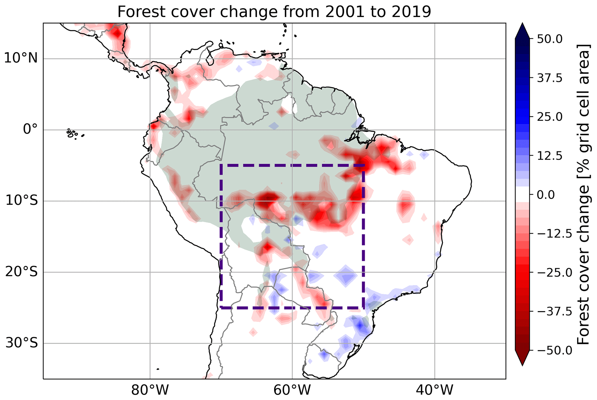
Figure 1 Change in forest cover (% of grid cell area deforested or re- or afforested) between 2001 and 2019 calculated using MODIS land cover data. The region analysed in this study is marked with the purple box.

2.2 Remote-sensing data sources

2.2.1 Land surface data

The Moderate Resolution Imaging Spectroradiometer (MODIS) land cover data at 0.05° resolution (product MCD12C1; Friedl and Sulla-Menashe, 2015) were chosen as a measure of vegetation type based on the long temporal record of annual data (Table 1) and a comparison of the magnitude and timing of Amazon deforestation in three land cover datasets (see the Supplement). The MODIS sensor operates on two satellites: Terra (launched in December 1999) and Aqua (launched in May 2002). For 2001–2020, the time period for which the data were used, the Terra and Aqua crossing times were, respectively, 10:30 and 13:30 local time. Both had sun-synchronous, near-polar orbits and an altitude of 705 km. The land cover data have been available since 2001 and combine retrievals from both satellites. From the multiple land cover classifications available in the MCD12C1 product, the 17-class International Geosphere–Biosphere Programme classification (IGBP; Loveland and Belward, 1997) was chosen for this project, as it has been used in relevant work, such as the FINNv2.5 fire emission inventory (Wiedinmyer et al., 2023). The C6 MODIS Land Cover product is assessed to have an accuracy of 73.6 % (Sulla-Menashe et al., 2019).

Table 1 Summary of satellite datasets analysed in the study. All datasets were analysed on 1° × 1° spatial resolution. Lifetimes are taken from Jacob (1999), Holloway et al. (2000), Pacifico et al. (2009), Hodzic et al. (2016), Wells et al. (2020), Bates et al. (2021), and Pommier (2023).

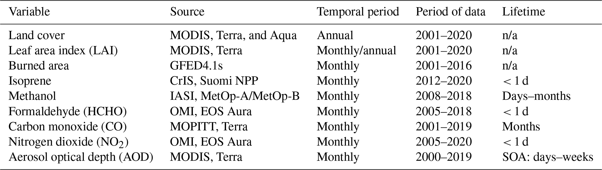
n/a: not applicable.​​​​​​​

The leaf area index (LAI) data are also a MODIS product (MOD15A2H; Myneni et al., 2021) and can represent vegetation abundance. The LAI product is based on measurements from the Terra satellite at an 8 d temporal resolution and, validated against ground measurements, has a root mean square error of 0.69 across all biomes (Devadiga and Nickeson, 2023). It has been available since February 2000 to the present day. We used the LAI product to calculate the annual and monthly mean values for the period 2001–2020 at 1° × 1° resolution in the Google Earth Engine (Gorelick et al., 2017).

The burned area to represent fire activity was obtained from version 4.1s of the Global Fire Emissions Database (GFED4.1s; Giglio et al., 2013). Monthly burned area is available at 0.25° spatial resolution from August 2000 to December 2016. The data for 2001–2016 were used in the analysis. For the period of interest, the GFED4.1s burned area is predominantly based on the MCD64A1 product, which has been found to have a 68 % burned area omission error (Padilla et al., 2015). However, GFED4.1s includes the addition of small fire burned areas, which likely counter some of the omission error, as the GFED4.1s burned area is 37 % greater than that of GFED3, which did not include small fire estimates (van der Werf et al., 2017). A summary of the land surface and atmospheric composition datasets is provided in Table 1.

2.2.2 Atmospheric composition data

Gridded total isoprene columns for 2012–2020 at 0.5° × 0.625° spatial resolution at monthly resolution were obtained from Wells et al. (2020). These data are derived from measurements taken using the Cross-track Infrared Sounder (CrIS), a Fourier transform spectrometer, on board the Suomi National Polar-orbiting Partnership (Suomi NPP) satellite. Suomi NPP was launched in October 2011 and has a sun-synchronous orbit and near-global twice daily coverage, with a daytime local overpass time of 13:30 LT. Isoprene column densities were calculated using two isoprene infrared absorption features in the spectral range 890–910 cm⁻¹. This novel data product has been quality assessed through comparison against ground-based isoprene column measurements in the Amazon, which found the retrieved isoprene column amounts differ by 20 % to 50 % when compared to ground-based column measurements (Fu et al., 2019; Wells et al., 2020, 2022).

The total column methanol data, another recently developed dataset, comes from the Infrared Atmospheric Sounding Interferometers (IASIs) on board the MetOp-A and MetOp-B satellites. These EUMETSAT MetOp satellites have/had (MetOp-A was deorbited in 2021) sun-synchronous polar orbits at an altitude of around 817 km and local overpass times of 09:30 and 21:30 LT. The daytime (09:30 LT) data for 2008–2018 were produced using the Infrared Microwave Sounding (IMS) scheme developed by the Rutherford Appleton Laboratory (RAL) (Pope et al., 2021). Pope et al. (2021) found a systematic difference of around 30 % compared to the Atmospheric Tomography Mission (ATom) flight measurements in areas of methanol enhancement, as well as an uncertainty of 40 % to 50 % for an individual sounding, which will have been reduced here by averaging.

HCHO and NO₂ are measured using the Ozone Monitoring Instrument (OMI) located on the Earth Observing System (EOS) Aura satellite. OMI employs spectrometers in visible and ultraviolet wavelengths and has provided daily global coverage since late 2004. Aura flies at 705 km and has an Equator-crossing time of 13:45 LT. Level 2 total column HCHO data were downloaded from the NASA Goddard Earth Sciences Data and Information Services Center (GES DISC; Chance, 2007). Only pixels with the “good” main quality flag, which includes checks of fit convergence, column uncertainty and absolute column value, and cloud cover of less than 20 %, were used to calculate monthly mean values. Uncertainties in individual retrievals of the HCHO columns range within 50 % to 105 %, with HCHO hotspots characterised by lower uncertainty values and averaging leading to uncertainty reduction (OMI Team, 2012). We found an underlying positive trend in the HCHO data, possibly associated with instrument degradation (Wang et al., 2022), and anomalous values in 2019. Consequently, only the HCHO data for 2005–2018 were used, and the monthly values were detrended based on a remote Pacific region (see the Supplement). This highlights local variations due to biogenic and pyrogenic emissions, as opposed to those driven by changes to the global background.

The tropospheric column NO₂ data are the Quality Assurance for Essential Climate Variables (QA4ECV) tropospheric NO₂ product (Boersma et al., 2011) available as global monthly averages at 0.125° × 0.125° spatial resolution. The data were downloaded for 2005–2020. The monthly mean values only include retrievals with cloud radiance fractions under 50 %, which is approximately equivalent to geometric cloud fractions under 20 %. Boersma et al. (2011) estimated the uncertainty for individual retrievals of the NO₂ tropospheric columns to be 1.0 × 10¹⁵ molec. cm⁻² + 25 % of the retrieval.

AOD is a measure of the light attenuation by atmospheric aerosols due to either absorbance or reflectance (Wei et al., 2020). Low AOD values (< 0.1) indicate a clear sky and low aerosol amounts, while values of 1 suggest very hazy conditions with high aerosol concentrations. Consequently, an increase in aerosol concentration, e.g. due to emissions of particles during combustion, should lead to higher AOD values. AOD is provided as part of a level 3 1° × 1° spatial resolution monthly product from MODIS measurements on board the Terra satellite (MOD08_M3; Platnick et al., 2015). Each monthly statistically derived dataset (SDS) is based on the relevant MODIS Atmosphere Daily Global Joint Product. The quality-controlled overland AOD data are available at three wavelengths: 0.47, 0.55, and 0.66 µm. AOD retrievals are expected to have errors within the $\pm \mathrm{0.05}+\mathrm{0.2}\times$ AOD value (Levy et al., 2013; Sayer et al., 2014). The 0.47 µm data for 2000–2019 are used throughout the analysis, as these were found to exhibit the strongest statistical relationship with the land variables (not shown).

The total column CO data are from the Measurement of Pollution in the Troposphere (MOPITT) sensor also on board the Terra satellite. Monthly mean values at 1° × 1° resolution were calculated for 2001–2019 from the version 7 level 2 product (NASA/LARC/SD/ASDC, 2000). The CO total column values have biases of less than 0.2 × 10¹⁸ molec. cm⁻² and standard deviations of around 0.2 × 10¹⁸ molec. cm⁻² compared to NOAA validation sites and a field campaign (Deeter et al., 2017). The data for 2000 was omitted due to large data gaps that year. Only clear-sky scenes are included in the MOPITT retrievals.

2.3 Analysis of remote-sensing data for the southern Amazon

All observational data were re-gridded to a 1° × 1° horizontal resolution using linear interpolation to provide spatially consistent datasets for analysis and inter-comparison. The atmospheric composition and burned area data were all analysed on a monthly temporal resolution, while the land cover and LAI data were annual, with the exception of calculating the LAI seasonal cycle. To better understand the impacts of seasonality, we separated the monthly data into wet (February, March, and April) and dry (August, September, and October) seasons. The 3-month intervals were chosen based on seasonal variations in precipitation and compatibility with previous definitions (Barkley et al., 2009; Reddington et al., 2015). The dry-season data were further separated into high-burned-area (monthly burned areas ≥ 0.04 % grid cell area) and low-burned-area grid cells. The threshold for defining the high burned area of ≥ 0.04 % was chosen to ensure sufficient sample sizes in each category, while identifying areas with clear fire signals (see the Supplement). There is a 6 km difference in elevation within the region with maximum elevations in the south west (SW). As some of the satellite retrievals are associated with high errors over the high altitudes of the Andes, a small portion of the domain > 1000 m a.s.l. was not included in our analysis.

Whenever data for different domains are compared (e.g. difference in isoprene over regions of low and high burned area at a given forest cover), the mean across all available data satisfying the domain conditions was calculated. First, the relevant datasets were subset in time, so the only years included are those for which land cover, burned area, and composition data are all available. Next, the data were split based on the burned area threshold. Each subset (high and low burned area) was then sorted into land cover bins, and then the mean and standard error for each bin were calculated.

Regression analysis was used to quantify the relationship between the following surface variables: land cover, LAI and burned area, and the atmospheric constituents. A Spearman rank correlation (Dodge, 2008),

$$\begin{array}{}\text{(1)}& r=\mathrm{1}-{\displaystyle \frac{\mathrm{6}{\sum }_{i=\mathrm{1}}^n{d}_i^{\mathrm{2}}}{n\left(n^{\mathrm{2}}-\mathrm{1}\right)}},\end{array}$$

where r is the Spearman rank correlation coefficient, n is the sample size, and d_i represents the difference between the ranks of the ith values from each sample. The ordinary least squared (OLS) and Theil–Sen regression methods (Fernandes and Leblanc, 2005) were utilised. The OLS regression aims to minimise the sum of the squared differences between the observations and the model (residual sum of squares) when fitting a linear model. The Theil–Sen regression is more robust to outliers than OLS regression, as it fits a slope and intercept based on the spatial median of these parameters calculated on subpopulations of the data. Where a clear relationship (OLS coefficient of determination (R²) ≥ 0.25) was identified between an atmospheric constituent and land cover or burned area, the data were binned by the explanatory variable, and a weighted least-squares (WLS) regression was used to account for the variance of the data in each bin. Throughout the text, we use standard errors to represent uncertainty ranges.

3 Results

3.1 Change in atmospheric constituents, land cover, and burned area through time

Over the early 21st century (2001–2019), forest cover averaged over the southern Amazon region decreases by 3.8 % from 52.0 % to 48.2 % of the study region (Fig. 2a). The deforestation is greatest in the north (N) of the domain at around 10° S (see Fig. 1). Generally across the region, forest cover reduces substantially from 2001 to 2013, with a smaller decline thereafter. Over the same period, savanna and grassland expand from 46.7 % to 50.5 % (Fig. 2b) (see the Supplement for the separated savanna and grassland time series). The two land cover categories, broadleaf forest and savanna and/or grassland, display opposite trends through time (Fig. 2a, b), reflecting that broadleaf forest cover is being replaced by the savanna/grassland modal land cover type.

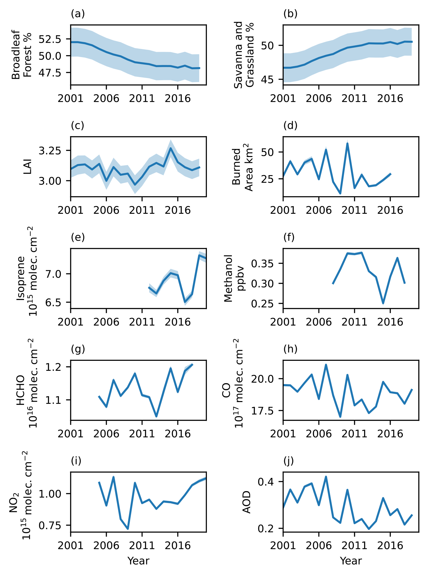
Figure 2 Annual mean values for (a) broadleaf forest cover percentage, (b) savanna and grassland cover percentage, (c) LAI, (d) burned area (based on monthly sums), and the atmospheric constituents. These include (e) isoprene, (f) methanol, (g) HCHO, (h) CO, (i) NO₂, and (j) AOD and are averaged for the southern Amazon region for all years available for each variable. The shading represents the standard error based on all data included in calculating the annual mean, i.e. the values of each grid cell for a given year for the land cover and LAI or the monthly values of each grid cell for the burned area and the atmospheric constituents. The larger amount of data used in calculating the mean values for panels (d)–(j) results in smaller standard errors.

Mean LAI and total annual burned area averaged over the study region do not have consistent trends over 2001–2019 and 2001–2016, respectively (Fig. 2c, d). Average annual LAI values in the region fluctuate around a value of 3.1, with a standard deviation of 0.06. As the regional estimate of LAI is dependent on all vegetation types in the domain, any decrease in LAI due to decreases in broadleaf forest (high LAI values) may be of a lesser magnitude than year-to-year variability in the vegetation overall due to, e.g., weather or disease. Burned area also exhibits substantial year-to-year variability, with maximum values observed in 2007 and 2010, while the least burning occurs in 2009. Since 2011, the monthly average burned area has remained below 200 km² in the peak burning months, and the inter-annual variability has decreased.

The year-to-year variability for annual regional mean CO, NO₂, and AOD is similar to that for the burned area (minima in 2009 and maxima in 2007 and 2010; Fig. 2h, i, j). These atmospheric constituents also show reduced year-to-year variability from 2011 onwards, with the exception of elevated values in 2015 for AOD and CO. The 2007 and 2010 maxima are also observed in the HCHO record, although the year-to-year variability does not reduce for this trace gas (Fig. 2g). The similarities in the temporal record suggest that the burned area has an influence on the domain-averaged AOD, CO, NO₂, and HCHO.

Methanol and isoprene are also characterised by substantial inter-annual variability, and neither shows a clear trend through time for the region average (Fig. 2e, f). Consequently, other annually varying factors affecting these constituents, such as meteorology or changes in other sources and sinks (Pacifico et al., 2009; Wohlfahrt et al., 2015), may have a greater impact than the decrease in broadleaf forest cover, which is limited in its spatial extent, over this time period. It is noted that the annual mean isoprene and methanol datasets do not extend as far back in time as the land cover dataset, and the change in broadleaf forest cover is smaller during the period covered by these datasets.

3.2 Seasonal cycle in atmospheric composition and burned area

The regional average seasonal cycles of the six atmospheric constituents are found to be similar with a peak in the dry season (August to October) for all species (Fig. 3). Uniquely, isoprene shows a secondary peak earlier in the calendar year in March/April, which is when the isoprene column densities reach 80 % of the annual maximum (August regional mean of 8.6 ± 0.5 × 10¹⁵ molec. cm⁻²).

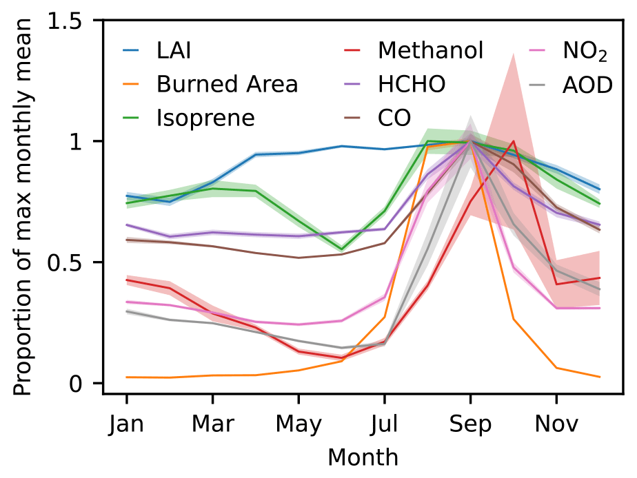
Figure 3 Seasonal cycles of domain-averaged LAI, burned area, isoprene, methanol, HCHO, CO, NO₂, and AOD for the periods where each dataset is available between 2001 and 2020. All variables have been normalised (to a value of 1) against their respective regional maximum monthly mean. The shaded areas represent the standard error for each variable for a given month.

Several of the constituents also have co-occurring minima. Isoprene, methanol, and AOD all have the lowest values of 4.7 ± 0.1 × 10¹⁵ molec. cm⁻², 0.1 ± 0.01 ppbv, and 0.11 ± 0.004, respectively, around June. HCHO, CO, and NO₂ remain more stable between December and June.

The amplitudes of the seasonal cycles of the different constituents vary. Isoprene, HCHO, and CO have relatively low intra-annual variation, as their column amounts remain above 50 % of their maxima throughout the year. In comparison, methanol, AOD, and NO₂ exhibit a more extreme seasonality, with values dropping below 30 % of their annual maxima. This pronounced dry-season peak in the atmospheric constituents is consistent with the burned area seasonal cycle, which rises from 0.02 ± 0.002 % of the study region in July to 0.06 ± 0.009 % in September, before decreasing to 0.02 ± 0.002 % again in October. Burned area values remain below 10 % of the September peak for the rest of the year.

The LAI seasonality is substantially different, as values remain above 70 % of the maximum throughout the whole year. LAI is elevated at > 3 (> 90 % of the maximum value) between April and October. The regional monthly mean drops slightly (< 2.7 or < 80 %) from December to February. The lower-percentage amplitude of the LAI seasonal cycle may be driven by different phenologies of the vegetation in the domain; e.g. the Cerrado savanna grassland flowering is relatively consistent throughout the year, while Amazon Rainforest vegetation tends to flower in the dry season (Morellato et al., 2013). Other research in Brazil has found that while seasonal changes in forests are associated with solar radiation, they are driven by rainfall for savannas and grasslands, resulting in opposite cycles for the different land cover types (Myneni et al., 2007). A comparison of six LAI datasets consistently shows that in the southern Amazon the LAI in regions of broadleaf forest cover is higher in July, compared to January, while the savanna/grassland region has the opposite LAI signal (Fang et al., 2013). Consequently, phenology-driven LAI values may peak at different times, depending on the land cover types, resulting in full/partial vegetation coverage of the region throughout the year.

The magnitudes of all atmospheric constituents examined in this study increase in the dry season when the burned area is largest, suggestive of changes to the atmospheric chemistry due to a substantial pyrogenic source. In particular, the seasonal variability in NO₂ and AOD closely matches the seasonality in the burned area, while methanol does so with a lag of 1 month. As outlined above, vegetation cover, as represented by the LAI, shows more consistent values throughout the year. Therefore, constituents with lower seasonal amplitudes are potentially more strongly linked to the seasonality of biogenic emission sources, although other factors such as atmospheric lifetime will have an important impact on the respective atmospheric constituent concentrations.

3.3 Spatial distribution of vegetation, fire, and atmospheric composition

Across the southern Amazon, broadleaf forest, savanna, and grasslands represent the dominant vegetation types. Annual average broadleaf forest cover dominates in the northwest (NW), with land surface coverage typically between 80 % and 100 %, while savannas and grasslands represent the main land cover (80 %–100 % coverage) in the southeast (SE) (Fig. 4). In the centre of the domain, a transitional region exists, where the competing phenologies typically have 40 %–60% coverage. The corresponding LAI spatial distribution highlights larger values (3.5 to > 5.0) in the NW and lower values (2.0–3.5) in the SE. This is consistent with broadleaf forest having a larger biomass (per unit area) in comparison to savanna/grassland vegetation types.

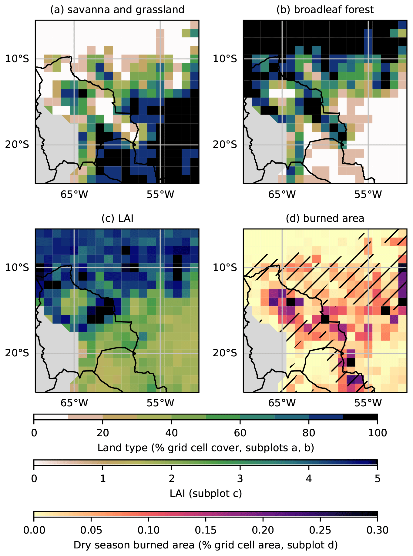
Figure 4 The annual mean distribution for 2001–2019 of (a) savanna and grassland and (b) broadleaf forest cover, represented as the percent of each grid cell covered by the respective land cover type, and (c) annual mean LAI for 2001–2019. Dry-season (August–October) monthly mean burned area (% grid cell area) for 2005–2016 is shown in panel (d), along with regions where at least 2.5 % of the area has been deforested marked by hatching. Areas over 1000 m a.s.l., based on the GMTED2010 digital elevation model (Danielson and Gesch, 2011), have been masked on all panels.

For the dry-season burned area data, there are sporadic hotspots peaking at > 0.3 %. The most coherent spatial structures are a filament of burned area values between 0.2 % and 0.3 %, stretching along the Bolivian eastern border down into Paraguay in the south (S) of the region, and the cluster of western Brazilian burned area values at > 0.1 %, peaking at 0.3 %–0.5 %. This latter feature is generally consistent with the reported “arc of deforestation” in the Amazon (Reddington et al., 2015; dos Santos et al., 2021). The hatching in Fig. 4d represents at least a 2.5 % decrease in broadleaf forest between 2001 and 2019, which coincides with the burned area patterns reported here. Therefore, the fire activity may be related to regions undergoing deforestation and, to a certain extent, the land cover classifications. For instance, the burned area filament in Fig. 4d closely follows the high (> 90 %) or low (< 20 %) savanna/grassland and broadleaf forest structure in Fig. 4a and b. Thus, it is suggestive of transitional regions between biomes driven by predominately anthropogenic pyrogenic activity. Overall, the spatial distribution of burned area exhibits more localised maxima than vegetation cover.

The spatial distributions of multi-annual mean values of total column isoprene are similar to those of broadleaf forest cover and LAI for both the wet and dry season (cf. Figs. 5a, b and 4b, c). Values decrease from the far NW (maximum of 2.7 × 10¹⁶ molec. cm⁻² in the dry season) to < 0.5×10¹⁶ molec. cm⁻² in the S, following the NW–SE transition from forest to savanna/grassland as evident in the dry-season total column isoprene values (see Figs. 4b and 5b). Over the broadleaf forest region, isoprene is elevated in the west (W), where the maximum forest cover occurs, compared to the east (E). The spatial similarities between broadleaf forest cover and total column isoprene amounts suggest that the broadleaf forest is the dominant source of this BVOC for this region, especially in the dry season. This finding is also consistent with the short lifetime of isoprene confining the peak concentrations to the source region. The W–E gradient in mean total column isoprene over the forested region itself suggests variability in the isoprene emissions within the broadleaf forest biome due to different plant species or local environmental conditions, as found by Gu et al. (2017), who identify an elevation gradient in isoprene emissions in the tropical forest N of the region studied here, probably driven by plant species distributions. In this study, the highest total column isoprene values occur at elevations of around 200 m a.s.l., with lower isoprene column densities in the N of the forest, where elevations decrease to below 100 m a.s.l.

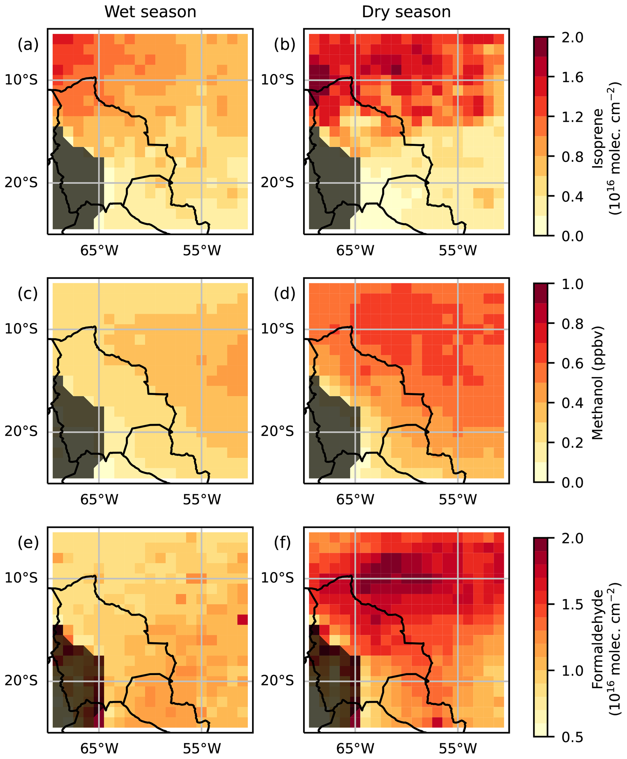
Figure 5 Regional distributions of column mean isoprene (a, b; molec. cm⁻²), methanol (c, d; parts per billion by volume – ppbv), and formaldehyde (e, f; molec. cm⁻²; note that the colour bar starts at 0.5 × 10¹⁶ molec. cm⁻²) for the wet season (a, c, e) and dry season (b, d, f). The wet season includes the months of February–April, while the dry season covers August–October. The time period varies with constituent. Areas over 1000 m a.s.l. based on the GMTED2010 digital elevation model (Danielson and Gesch, 2011) have been masked on all panels and are not included in further analysis.

Two other atmospheric constituents, namely CO and AOD, have similar distributions in the wet season to that of broadleaf forest cover. CO is elevated in the NW (> 16×10¹⁷ molec. cm⁻²; maximum of 18.2 × 10¹⁷ molec. cm⁻²), compared to the SE (< 14 × 10¹⁷ molec. cm⁻²). AOD is similarly elevated in the N (> 0.2, maximum of 0.35) and reaches a minimum in the SE of the study region (< 0.1) (Fig. 6a, c). The spatial patterns of CO and AOD during the wet season are consistent with the broadleaf forest acting as a source of biogenic precursors of CO and aerosols as values increase over more densely forested areas (compare with Fig. 4b). This is consistent with biogenic sources having a greater relative impact on CO and aerosols in the wet season, which is when pyrogenic emissions are minimal (Artaxo et al., 2022).

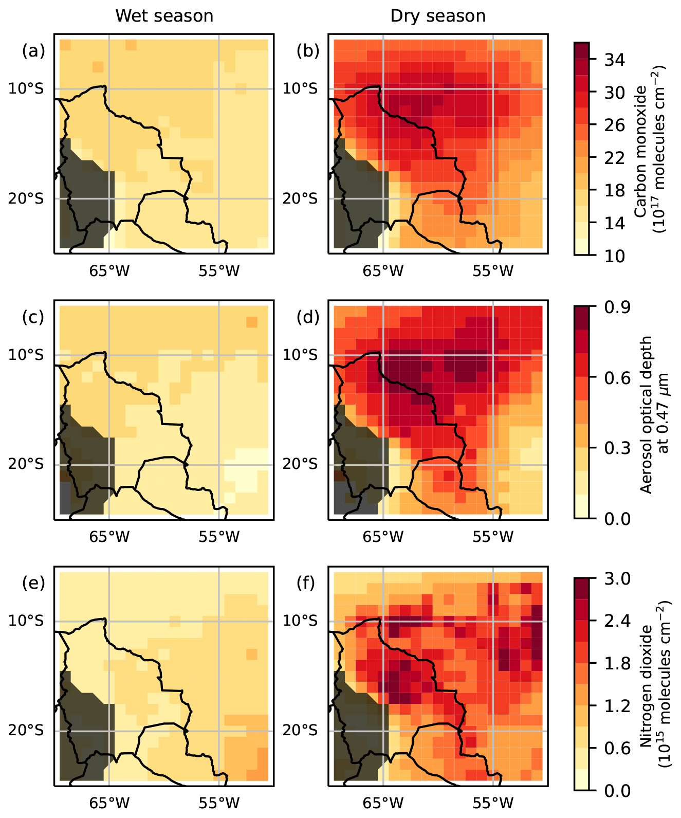
Figure 6 Regional distributions of CO (a, b; molec. cm⁻²; note that the colour bar starts at 10 × 10¹⁷ molec. cm⁻²), AOD (c, d), and NO₂ (e, f; molec. cm⁻²) for the wet season (a, c, e) and dry season (b, d, f). The wet season includes the months of February–April, while the dry season covers August–October. The time period varies with constituent. Areas over 1000 m a.s.l., based on the GMTED2010 digital elevation model (Danielson and Gesch, 2011), have been masked on all panels and are not included in further analysis.

In contrast, wet-season HCHO and NO₂ increase from the NW (HCHO and NO₂ column values of ∼ 0.8 × 10¹⁶ and < 0.6 × 10¹⁵ molec. cm⁻², respectively) to the SE, where HCHO reaches a maximum of 3.2 × 10¹⁶ molec. cm⁻² and NO₂ is 1.36 × 10¹⁵ molec. cm⁻². This spatial pattern is not consistent with biogenic emissions from the forest being the dominant controlling factor (Figs. 5e and 6e; compare to Fig. 4b). Furthermore, biomass burning is minimal in the wet season (see Sect. 3.2), suggesting that another source or sink is driving total column HCHO and tropospheric column NO₂ in this season. The wet-season methanol concentrations are also different to that of vegetation cover. The highest methanol concentrations of ≥ 0.4 ppbv are recorded in the far E of the domain between 10 and 16° S (Fig. 5c).

The dry-season spatial patterns of HCHO, CO, and AOD differ somewhat from their wet-season distributions, suggesting a change in dominant sources/sinks e.g. from vegetation to fires, transport, and/or atmospheric chemistry processes. CO appears more well-mixed compared to the other trace gases, as expected, with its relatively longer lifetime compared to the other species (average CO tropospheric lifetime of 1–3 months; Seinfeld and Pandis, 2016; compare with Table 1) (Fig. 6b). HCHO, CO, and AOD reach maximum values (up to 3.7 × 10¹⁶ molec. cm⁻², 32.7 × 10¹⁷ molec. cm⁻², and 0.88, respectively) over the transition zone between forests and other land cover classes, although the exact locations of these peaks vary. This region is most strongly affected by deforestation and proximate to the highest average dry-season burned areas (compare with Fig. 4). Total column HCHO decreases beyond this zone, consistent with a significant pyrogenic source (Freitas and Fornaro, 2022; Palmer et al., 2007), both further into the broadleaf forest (1.2 to 1.6 ×10¹⁶ molec. cm⁻²) and to the S, where values drop to < 0.6 × 10¹⁶ molec. cm⁻² (Fig. 5f). Minima in the AOD and CO data are also found in the S at the foot of the Andes and in the SE (< 0.2 and < 18 × 10¹⁷ molec. cm⁻², respectively) (Fig. 6d). Peak total column CO is found slightly further S to the HCHO maximum (10–12° S compared to 8–11° S). AOD is characterised by two maxima (> 0.8), within the same region as CO, which occur in areas of mixed land cover (forest cover 10 %–100 %) that have experienced substantial deforestation (> 2.5 % area deforested) and some burning (dry-season monthly mean burned area ∼ 0.01 %) (compare Figs. 6d and 4). However, this does not correspond to the locations of maximum dry-season burned areas. The co-location of these maximum values with regions of deforestation and biomass burning suggests that a pyrogenic source, potentially emissions from deforestation fires, is important for these constituents. These constituents were also elevated to the N of this region, where the forests are dominant, suggesting the presence of a biogenic source for this region or the transport of pyrogenic emissions. Particularly in the case of HCHO, the presence of NO_x associated with biomass burning could affect the HCHO yield from BVOC emissions (Langford et al., 2022), potentially increasing HCHO formation from isoprene oxidation over the broadleaf forest.

Methanol dry-season concentration values are similarly elevated (> 0.6 ppbv) in the N over the forest to savanna–grassland transition, but they are also consistently high further into the Amazon Rainforest, as well as in the NE. Some of the maxima are located over areas of mixed vegetation, which experienced substantial deforestation over 2001–2019, as found for HCHO, CO, and AOD (compare Fig. 5d with Figs. 1 and 4), but other regions do not reflect any of the studied land surface variables.

The dry-season NO₂ column densities had several distinct maxima > 2.7 × 10¹⁵ molec. cm⁻², with the highest being 3.5 × 10¹⁵ molec. cm⁻², which are all located 9–16° S. Some of these overlap with the two AOD maxima. Unlike AOD, NO₂ is clearly elevated over the maximum burned areas recorded at 15° S, 65° W and in the E of the study region (Figs. 6d, f and 4d). In regions of minimal fire activity, such as deeper into the Amazon Rainforest and the edge of the Andes, tropospheric column NO₂ is < 0.9 × 10¹⁵ molec. cm⁻². The spatial pattern of the tropospheric column NO₂ closely resembles that of burned area, highlighting the close relationship between the trace gas and fire activity, owing to its much shorter lifetime (around 1 d for NO_x at the surface; Jacob, 1999) compared to CO and aerosols.

3.4 Influence of vegetation and fire on atmospheric composition

3.4.1 Variations in atmospheric composition with broadleaf forest cover

In this section, the variation in the atmospheric composition as a function of broadleaf forest cover (i.e. percentage cover in 10 % bins) is considered for the dry and wet seasons over the whole region and the time period of co-existing data. Within the dry season, the impact of pyrogenic activity is assessed by splitting the atmospheric constituent data into “low fire” (≤ 0.04 % burned area) and “high fire” (> 0.04 % burned area) regimes. Our results are relatively insensitive to the burned area threshold, as well as the bin width choice (see the Supplement).

Isoprene consistently increases with higher broadleaf forest cover in all four regimes (Fig. 7a). The spatial distributions rather than temporal variations drive this signal. Values are lower in the wet season (approximately 0.5–0.7 × 10¹⁵ molec. cm⁻²) than the dry season for broadleaf forest cover values > 20 %. In densely forested areas (broadleaf forest cover > 90 %), the dry-season isoprene column density is 50 % greater than in the wet season at approximately 1.0–1.5 × 10¹⁵ molec. cm⁻². The greater change between seasons in isoprene column amounts at higher forest cover suggests that isoprene emissions from broadleaf forest have a stronger seasonality than those from other vegetation types. The differences in mean isoprene column densities between areas of high and low fire activity remain within 0.3 × 10¹⁵ molec. cm⁻². Consequently, isoprene responds to the change in forest cover more than the change in burned area, highlighting the importance of its biogenic source, as suggested in Sect. 3.3.

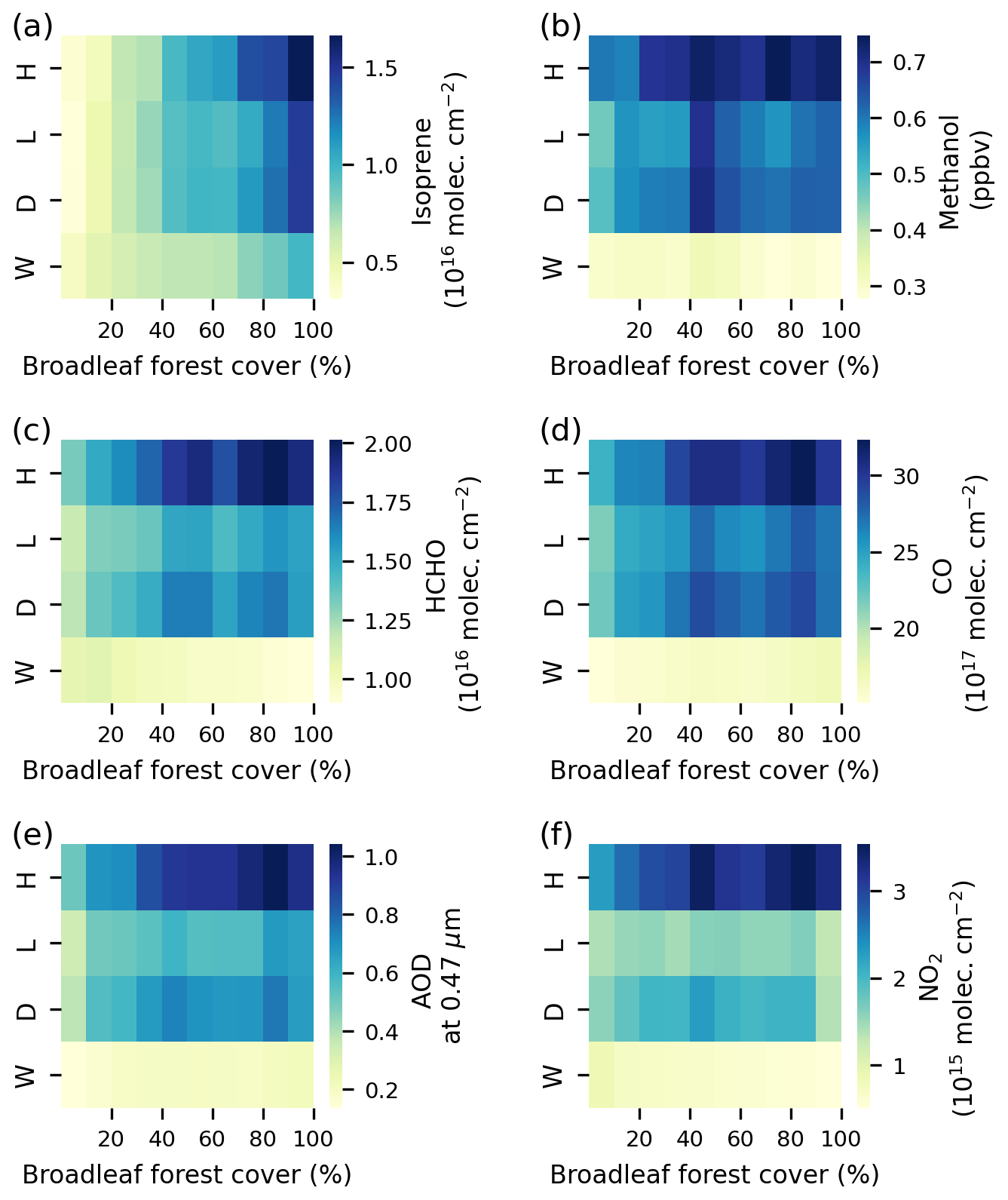
Figure 7 Mean monthly atmospheric constituent values, depending on percentage broadleaf forest cover in a given grid cell, for four categories: high burned area dry season (H), low burned area dry season (L), dry season (D), and wet season (W). Each subplot shows data for one atmospheric constituent, namely (a) isoprene (1 × 10¹⁶ molec. cm⁻²), (b) methanol (ppbv), (c) HCHO (1 × 10¹⁶ molec. cm⁻²), (d) CO (1 × 10¹⁷ molec. cm⁻²), (e) AOD, and (f) NO₂ (1 × 10¹⁵ molec. cm⁻²). Each subplot includes data for years when the given atmospheric constituent, land cover, and burned area datasets overlap.

For NO₂, a similar pattern occurs with larger column values in the dry season (approximately 1.5–2.0 × 10¹⁵ molec. cm⁻²) than in the wet season (≤ 0.86 × 10¹⁵ molec. cm⁻²) (Fig. 7f). However, the relationship with forest cover is non-linear, with peak dry-season column NO₂ in the 40 %–50 % forest cover bin. When split into the two fire regimes, there is a large column NO₂ difference independent of forest cover bin. When fires are low, the tropospheric column NO₂ ranges between 1.2 and 1.3 × 10¹⁵ molec. cm⁻², while in the high fire regime all column NO₂ values are > 2.5 × 10¹⁵ molec. cm⁻² (i.e. at least 60 % larger). Overall, as noted in Sect. 3.3, this result is suggestive of the largest NO₂ emissions from pyrogenic sources in forested regions and/or transition zones between vegetation types.

Consistent with the other constituents, column methanol values are larger (0.5–0.7 ppbv) in the dry season than the wet season (< 0.3 ppbv). While the low fire regime is very similar to the dry-season average, the high fire regime column methanol values are larger (≥ 0.6 ppbv) for all forest cover bins. Similar to NO₂, though, the peak values are in the 40 %–50 % and 70 %–80 % forest cover bins (Fig. 6b). Therefore, unlike for isoprene, the methanol columns are not linearly linked to forest cover, but typically, a larger forest cover percentage bin will have larger methanol values.

The other atmospheric constituents (Fig. 7c, d, e) also have some similarities with both isoprene and NO₂. The wet-season values are much lower than those in the dry season, regardless of forest cover, consistent with the seasonal cycle of the regional averages discussed in Sect. 3.2. In the dry season, HCHO, CO, and AOD increase as forest cover increases from 0 % to 50 %, and values remain elevated at higher forest covers (≥ 1.5 ×10¹⁶ molec. cm⁻², > 25.7 ×10¹⁷ molec. cm⁻², and > 0.55, respectively, for forest cover > 50 %). The high fire regime is associated with higher values of the atmospheric constituents compared to the low fire regime across all forest cover values. HCHO is elevated by at least 13 %, AOD by 27 %, and CO by 7 %–17 %. The overall maxima are associated with both the high burned area and high forest cover of 80 %–90 %. In the dry-season average, a secondary maximum occurs for the 40 %–50 % (40 %–60 % for HCHO) forest cover bin, resembling that of the peak in NO₂ and methanol values. This result suggests that both vegetation and fire are important in driving the concentration of HCHO, CO, and aerosols in the region in the dry season through a combination of biogenic emissions, particularly from the forest, and pyrogenic emissions in the transition zone and in forested regions, strengthening conclusions drawn from the analysis of spatial maps in Sect. 3.3.

3.4.2 Variations in atmospheric composition with burned area

In this section, the change in the atmospheric constituents with burned area is analysed, depending on season (W – wet season; D – dry season) and, for the dry season, dominant land cover (F – ≥ 50 % forest cover; S – < 50 % forest cover; i.e. ≥ 50 % savanna/grassland).

Although isoprene total column amounts are increased during the dry season, when fire activity is at its highest in the southern Amazon (see Sect. 3.2), there is no clear relationship between the burned area extent and the isoprene column amount (Fig. 8a), as the highest dry-season total column isoprene values occur at 0 %–0.01 % (0.9 ± 0.01 × 10¹⁵ molec. cm⁻²) and 0.08 %–0.09 % (0.9 ± 0.1 × 10¹⁵ molec. cm⁻²) burned area. The data do further highlight the relevance of the land cover type for this trace gas. Regardless of the amount of burning, for each respective burned area bin, the total column isoprene is at least 140 % higher in regions of dominant forest cover than in regions dominated by savannas and grasslands. Therefore, the forest cover is closely connected to isoprene emissions, supporting conclusions reached in Sect. 3.4.1, suggesting that the broadleaf forest is the dominant source of this BVOC in the region in the dry season, while the pyrogenic source, limited in its spatial extent, has a more minimal influence, despite the dry-season maximum (see Sect. 3.2).

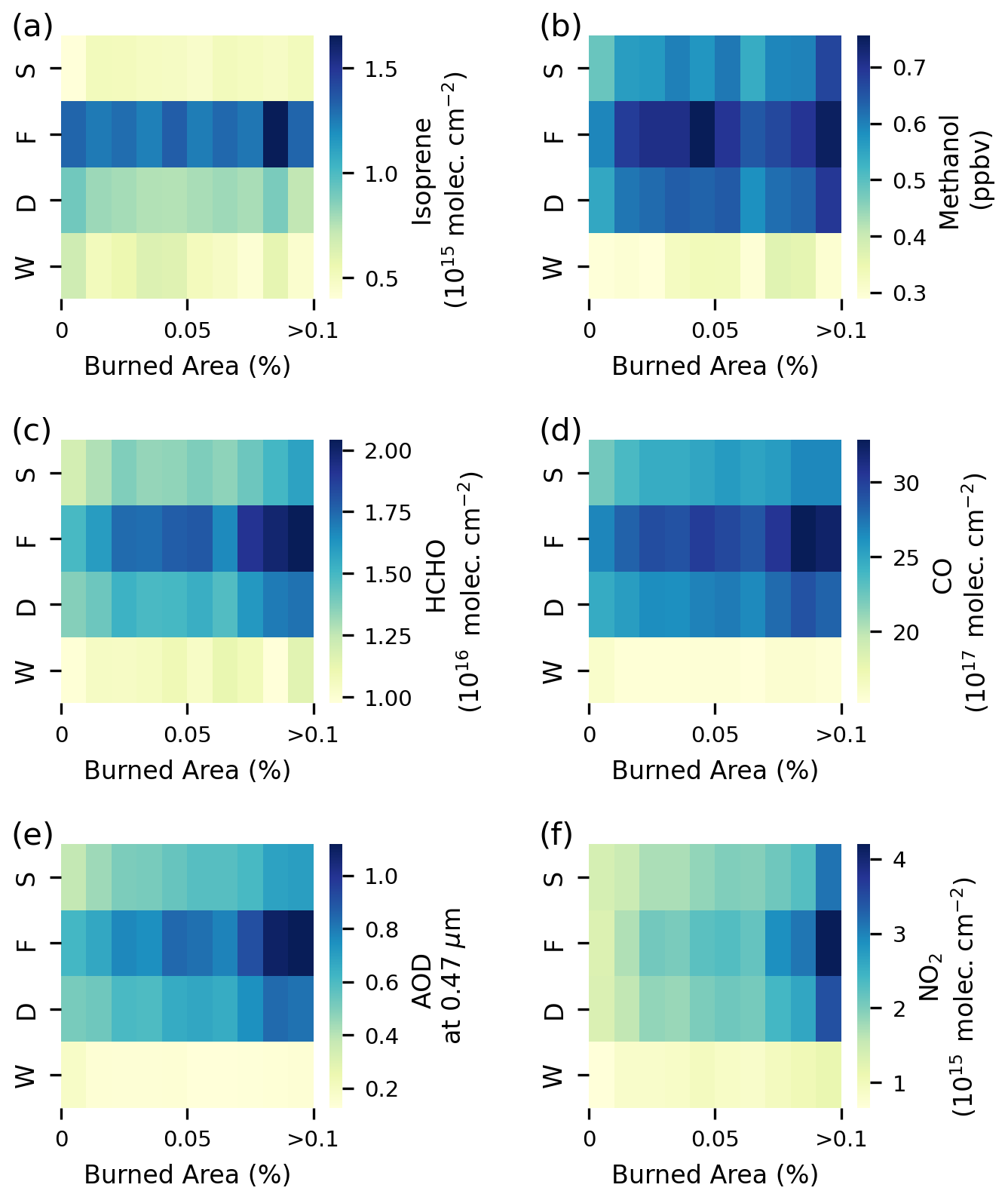
Figure 8 Mean monthly atmospheric composition depending on the percentage of burned area in a given grid cell for four categories: savanna-/grassland-dominated dry season (S), forest-dominated dry season (L), dry season (D), and wet season (W). Each subplot shows data for one atmospheric constituent, namely (a) isoprene (1 × 10¹⁶ molec. cm⁻²), (b) methanol (ppbv), (c) HCHO (1 × 10¹⁶ molec. cm⁻²), (d) CO (1 × 10¹⁷ molec. cm⁻²), (e) AOD, and (f) NO₂ (1 × 10¹⁵ molec. cm⁻²). Each subplot includes data for years when the given atmospheric constituent, land cover, and burned area datasets overlap.

The other constituents are also elevated over the forested area, compared to the savanna/grassland region, although the relative difference in the atmospheric constituent between the savanna/grassland and forest categories varies. This difference is particularly pronounced for HCHO and AOD (Fig. 8c, e). HCHO and AOD total column amounts over forests (1.5–2 × 10¹⁶ molec. cm⁻² and 0.6–1.1) are, respectively, ≥ 24 % and ≥ 35 % higher than those over savannas/grasslands. NO₂ has the smallest difference in values between the land cover categories (1.4–3.1 × 10¹⁵ molec. cm⁻² for savanna/grassland; 1.3–4.2 × 10¹⁵ molec. cm⁻² for forest) (Fig. 8f). For NO₂, AOD, CO, and HCHO, the differences between land cover types increase at higher burned area values.

The increase in atmospheric constituents over the forest compared to other land cover types may be driven by the emission of biogenic precursors and/or higher pyrogenic emissions when forest vegetation, as opposed to savanna/grassland, is burned. The latter is particularly relevant for NO₂, as the difference in the column densities between the land cover categories is only significant at high burned area values. At > 0.09 % burned area, NO₂ reaches 4.2 ± 0.1 × 10¹⁵ molec. cm⁻² over forest compared to 3.1 ± 0.1 × 10¹⁵ molec. cm⁻² over savanna/grassland.

On average, most of the same atmospheric constituents (NO₂, AOD, CO, and HCHO) increase with burned area in the dry season, reaching peak values at 0.08 %–0.09 % burned area (AOD and CO) or > 0.09 % burned area (NO₂ and HCHO). For methanol, the increase with burned area is limited to values of burned area under 0.05 %. The greater column amounts of these constituents associated with both forest cover and burned area are consistent with the dry-season maxima observed in (or proximate to) forested regions and over burned areas on the spatial maps in Sect. 3.3.

Consequently, all studied atmospheric constituents are influenced by the land cover type, as their abundances increase over more densely forested areas. Additionally, maximum values are reached in the presence of burning, especially at ≥ 0.07 % burned area for HCHO, CO, AOD, and CO in forested regions, showcasing the pyrogenic source. At low burned area values, there is little difference between forests and savannas/grasslands for NO₂, highlighting that burning is the major source of the trace gas in the region during the dry season, and the role of land cover is to modify the emissions where burning occurs.

3.5 Statistical relationships among atmospheric composition and land cover, LAI, and fire

In this section, statistical relationships between land cover, LAI, and burned area and the atmospheric constituents for the dry season are explored to quantify the extent to which land cover variables drive atmospheric composition over the southern Amazon for the time period during which both datasets are available. The Spearman rank correlation (Table 2) and OLS regression (Table 3; see Sect. 2) are utilised. The results from both methods are very similar, with the squared Spearman rank correlation coefficients slightly higher than the equivalent OLS R² values.

Table 2 Spearman rank correlation coefficients r (with the Spearman rank correlation coefficient squared, r², for comparison with Table 3 in parentheses). For each correlation, data for the 3 dry-season months for years when the atmospheric constituent and surface variable datasets overlap are used. In the case of annual vegetation data, all months of a given year are assumed to have the same vegetation cover. All r values are significant at the p = 0.05 level.

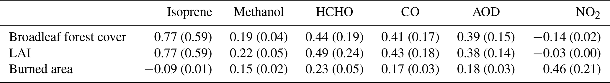
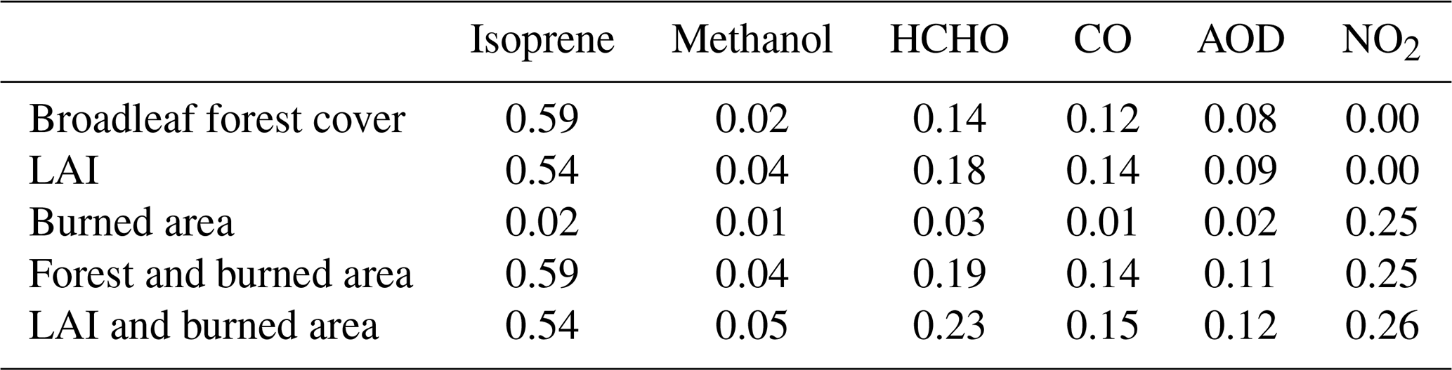
Table 3 OLS regression coefficients of determination (R²) for the dry season for single and multiple linear regression calculations. For each regression, data for the 3 dry-season months for years when the atmospheric constituent and surface variable datasets overlap are used. In the case of annual vegetation data, all months of a given year are assumed to have the same vegetation cover. All R² values are significant at the p = 0.05 level. The equivalent scatter plots for the data used to derive the linear OLS coefficients for broadleaf forest cover vs. isoprene and burned area vs. NO₂ are shown in Figs. 9a and 10, respectively.

There is a strong significant positive relationship between the two vegetation variables of broadleaf forest cover and LAI and total column isoprene over the region (Spearman's r = 0.77; OLS R² = 0.59 and 0.54 for broadleaf forest cover and LAI, respectively), as expected based, on Sect. 3.3–3.4.2. However, there is a weak negative relationship between isoprene and burned area. In contrast, tropospheric column densities of NO₂ exhibit a moderate positive relationship with burned area (Spearman's r = 0.46; OLS R² = 0.25) but a weak relationships with land cover variables over the region.

The relationships for the other atmospheric constituents are mixed and much weaker. HCHO, CO, and AOD all show positive weak to moderate relationships with both broadleaf forest cover and LAI (r values around 0.4; OLS R² = 0.08 to 0.18), suggesting some influence of vegetation on these atmospheric constituents, particularly for HCHO. The relationships between these atmospheric constituents and the burned area are considerably weaker but also positive (r values from 0.17 for CO to 0.23 for HCHO; OLS R² between 0.01 and 0.03). Methanol showed a similarly weak positive relationship with both land cover and fire (r values from 0.15 with burned area to 0.22 with LAI; OLS R² between 0.01 and 0.04). These weak results, compared to the isoprene relationship with vegetation, highlight that with the longer lifetimes of these trace gases and aerosols, especially CO and methanol (average lifetimes of 1–3 months and 5 d, respectively; Seinfeld and Pandis, 2016; Bates et al., 2021), there is more transport and mixing.

Multiple OLS regression was also performed to test whether the combination of biogenic and pyrogenic sources improved their explanatory power for the variation in atmospheric constituents. The R² value is unchanged for isoprene, while for NO₂, the R² values are minimally affected, suggesting one main emission source of vegetation and fire, respectively, for these two atmospheric species. For the other atmospheric constituents, the combination of broadleaf forest cover or LAI and burned area increased the R² values (compared to the OLS linear regression results) modestly. The change is most notable for HCHO (R² value of 0.23 compared to 0.18) and then for AOD (R² value of 0.12 compared to 0.09). While the overall R² values are still much lower than the R² value for the linear relationship between isoprene and broadleaf forest cover, for HCHO the multiple regression R² values are only slightly lower than for the NO₂–burned area relationship. This illustrates the relevance of both a biogenic and pyrogenic source to HCHO column densities, as previously observed elsewhere in Brazil (Freitas and Fornaro, 2022).

The more robust relationships between broadleaf forest cover vs. isoprene and burned area vs. NO₂ were studied in more detail (Figs. 9a and 10). The dry-season composition data were binned based on broadleaf forest cover (for isoprene) or burned area (for NO₂). We used a bootstrapping approach to test the significance of the isoprene (NO₂) increase with broadleaf forest cover (burned area) and found that the results are significant at the 95 % confidence level (not shown). Over the region, both binned (at 10 % broadleaf forest cover intervals) and non-binned data suggest that isoprene increases by 1.1 × 10¹⁵ molec. cm⁻² for every 10 % increase in broadleaf forest cover in the dry season (OLS R² = 0.59; WLS R² = 0.97) (Fig. 9). Consequently, the values for total isoprene column densities over completely (100 %) forested regions are on average 4 times greater than over non-forested regions (0 %). In non-forested regions, isoprene concentrations reflect the local background arising from emissions from non-forest species, as well as mixing and transport of forest-related emissions on short timescales. Tree species composition, in addition to forest dynamics and environmental conditions affecting the plant's emission efficiency, could explain the variability in the isoprene column amounts within each forest cover bin.

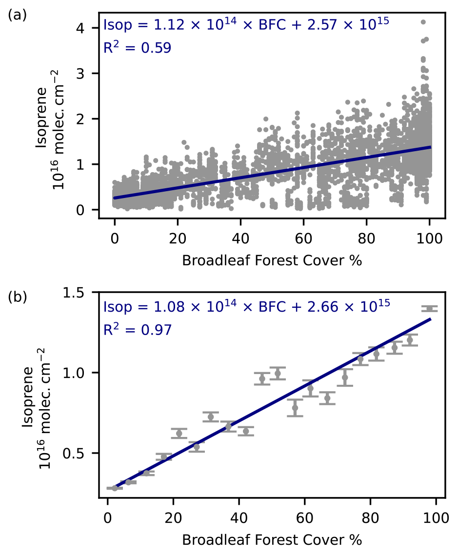
Figure 9 The relationship between dry-season monthly isoprene data and broadleaf forest cover (BFC) for 2012–2016 with the best-fit ordinary least square (OLS) regression line (a). Dry-season isoprene data for the same time period are binned based on 10 % broadleaf forest cover intervals with weighted least squares (WLS) regression results. The error bars show the standard error for each land cover bin (b). In panels (a) and (b), the text gives the best-fit linear regression equations.

The linear burned area–NO₂ relationship was found to exhibit different sensitivities, depending on vegetation cover (Fig. 10). Over regions of high forest cover and high LAI values, tropospheric NO₂ increases with burned area more than over locations with low forest cover and lower LAI (i.e. those dominated by savannas and grasslands; see Sect. 3.4.2). These different sensitivities are particularly clear up to around 0.5 % burned area (Fig. 10; see Fig. 8f for average conditions for burned areas from 0 % to > 0.1 %). Extremely high burned areas tend to occur in less forested regions, though the spatial distributions (Fig. 4) suggest that these are savanna/grassland fires proximate to the broadleaf forest in the central part of the region. The dominance of savanna/grassland at extremely high burned areas could decrease the variation in NO₂ explainable by the forest cover over the whole dataset (Tables 2 and 3).

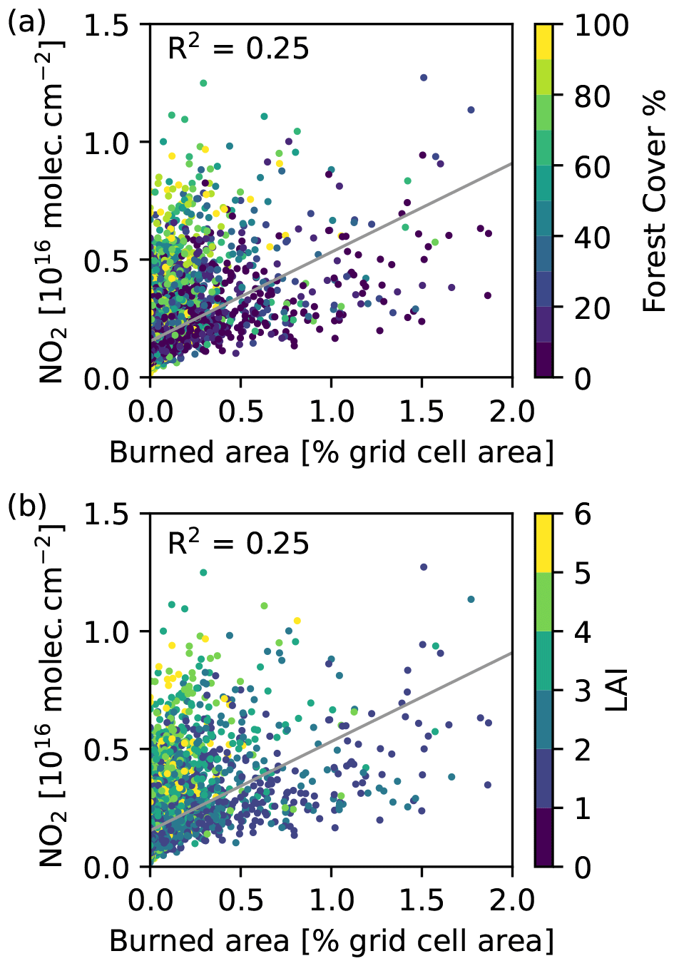
Figure 10 The distribution of monthly dry-season tropospheric NO₂ columns against monthly dry-season burned area percent coloured by broadleaf forest cover (a) and LAI (b) for 2005–2019. The panels display the OLS regression line and associated R² value, as included in Table 3.

Hence, to represent this more complex burned area–NO₂ relationship, we also explored the log–log relationship for NO₂ (log _e(NO₂)) and burned area (log _e(BA)) (R² = 0.32 for non binned data; WLS R² = 0.90 for binned data (at 0.25log _e(BA) intervals); Fig. 11). This log–log relationship, approximately a fifth root power law, indicates that the change in tropospheric column NO₂ is slightly greater at low burned area percentages compared to at high burned areas. This is consistent with the findings for the different vegetation types outlined above. The relationship was found to remain relatively consistent through time by testing the relationship between the natural logarithm of burned area from GFED5 (Chen et al., 2023) and natural logarithm of the NO₂ tropospheric column for the later time period 2017–2020 (not shown). For both NO₂ and isoprene, the WLS linear regression results were largely unaltered when the bin sizes were halved or doubled (not shown).

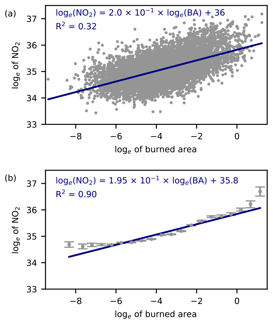
Figure 11 Natural logarithm of the monthly dry-season NO₂ data (log _e(NO₂)) against the natural logarithm of the monthly dry-season burned area (log _e(BA)) for 2005–2016 with the results of the OLS regression (a). The WLS regression analysis on the natural logarithm of monthly dry-season NO₂ data are binned based on the natural logarithm of the monthly burned area percentage cover for the same time period (b). The error bars show the standard error for each burned area bin. In panels (a) and (b), the text shows the best-fit equation found by the regressions and the respective R² value.

4 Discussion and conclusions

This study used new and complementary satellite observations to investigate the relationships between land cover, LAI, and burned area; five trace gases (isoprene, methanol, HCHO, CO, NO₂); and AOD in the southern Amazon, with the aim to understand the influence of vegetation and fire on atmospheric composition in a region of land cover change.

Biomass burning is identified as a potential driver of year-to-year variability in several trace gases, namely CO, HCHO, and NO₂, as well as aerosols, as suggested by the AOD record. Previous studies have identified drought years in 2005, 2007, 2010, 2012, and 2015 for this region (Pope et al., 2020; Panisset et al., 2018; Reddington et al., 2015), which may increase burning and modify the relationship between the burned area and emitted trace gases and aerosols. Although 2007 and 2010 are clearly elevated for burned area, AOD, CO, NO₂, and HCHO, not all of the listed drought years show maxima for a given variable in this study.

Pyrogenic sources in the dry season may further drive the seasonal cycle maxima of most of the atmospheric constituents over the region. The observed mean monthly isoprene seasonal cycle differs from the other constituents with a likely vegetation-driven secondary peak in the wet season. The isoprene seasonality is consistent with greater photosynthetically active radiation (PAR) in the dry season, as well as potentially greater isoprene emissions in response to water stress (Yáñez-Serrano et al., 2020). The isoprene minimum observed here in June has been previously linked to new leaf growth in the tropical forest in the transition between the wet and dry seasons, as young leaves start producing isoprene only after a few weeks (Barkley et al., 2009). The dry-season peak for HCHO in September is also consistent with a previous satellite study; however, a secondary wet-season peak was found in that work (Barkley et al., 2009). A weaker relationship between isoprene and HCHO is suggested for this region, since HCHO does not appear to respond to the variations in isoprene at the end of the wet season.

The spatial distributions across the southern Amazon further highlight the co-location of isoprene with broadleaf forest cover and high LAI and NO₂ with burned area. Most of the other atmospheric constituents show characteristics of both distributions. Methanol is unusual, due to a greater region of elevated column values in the N and NE of the region.

Broadleaf forest cover (LAI) explains 59 % (54 %) of the variation in the total column isoprene across the study region for the dry season over 2012–2019, which increases to 97 % when the isoprene data are binned based on 10 % forest cover bins. In the dry season, isoprene column amounts increase linearly with tree cover. For every 10 % increase in the broadleaf forest cover, the isoprene total column amount increases by 11×10¹⁵ molec. cm⁻² or around 40 % of the average background (0 % broadleaf forest cover) total column isoprene. This result is consistent for both the binned and original data.

In contrast, the burned area explains 25 % of the variability in the tropospheric column NO₂ for the dry season. In total, 32 % of the NO₂ variability can be explained when the natural logarithms of each variable are used, and the relationship is well-captured when these data are binned at 0.25log _e(BA) intervals (R² = 0.90). There is a stronger increase in the trace gas at lower burned area values, which is captured by the fifth root power law. Additionally, the NO₂ amount varies, depending on burning location, with greater values of NO₂ for an equivalent burned area in regions with at least 50 % broadleaf forest cover. These results are in agreement with the FINNv2.5 emissions inventory, which has larger biomass-burning emission factors for tropical forest compared to savanna/grassland (Wiedinmyer et al., 2023). However, the burned areas can be greater where tree cover is more sparse, highlighting the potential for substantial pyrogenic emissions from both forest and savanna/grassland regimes.

In the wet-season low tropospheric column, NO₂ values over the forested region and higher values in the SE could be driven by the forest canopy acting as an NO₂ sink through biological uptake, as suggested by Kang et al. (2023). Alternatively, a further NO_x emission source, e.g. from soils associated with agricultural activities (Wong and Geddes, 2021) or long-range transport of anthropogenic emissions in the region of São Paulo (van der A et al., 2008), may influence NO₂ concentrations.

The clear dry-season relationships of isoprene with broadleaf forest cover and NO₂ with burned area contrast with the mixed signals for the other atmospheric constituents. However, the combination of broadleaf forest cover and burned area can explain 23 % of the variation in dry-season total column HCHO, suggesting interactions between pyrogenic and biogenic emissions of HCHO and its precursors. The moderate correlation values of AOD and CO with the land cover variables suggest some influence of vegetation through a biogenic source that yields CO and SOA formation in August–October, although forest emissions are most relevant in the wet season (Yáñez-Serrano et al., 2020; Artaxo et al., 2022). Methanol does not exhibit a strong relationship with any land surface variable despite some observed similarities.

A key difference between methanol, AOD, and CO and isoprene, HCHO, and NO₂ is their lifetime. While isoprene, HCHO and NO₂ have lifetimes of up to a day (Pacifico et al., 2009; Wells et al., 2020; Pommier, 2023; Jacob, 1999), aerosol, methanol, and CO atmospheric lifetimes range from several days to months (Bates et al., 2021; Hodzic et al., 2016; Holloway et al., 2000). The extended time period that the aerosols, methanol, and CO are present in the atmosphere will increase the role of transport in the observed distribution, resulting in a less clear local source signal. These longer-lived species, particularly CO and aerosols, can therefore be transported from more distant anthropogenic sources (e.g. Park et al., 2015; Wang et al., 2015). However, anthropogenic emissions are thought to be minor compared to pyrogenic and biogenic sources in the study region. Anthropogenic sources are in the SE of the study area and beyond the region of interest, e.g. the large agglomerations of São Paulo and Rio de Janeiro located further to the SE (see, e.g., the European Commission, 2023, EDGAR v6.1 Global Air Pollution Emissions database).

The findings confirm the tropical broadleaf forest, as opposed to other vegetation types, as the dominant source of isoprene in the region, consistent with tropical trees being the dominant source of isoprene globally (Guenther et al., 2012). NO₂ is predominantly driven by pyrogenic emissions in the dry season, although the land cover type modulates the emission amount. HCHO, and to a lesser extent CO and aerosols, is linked to both biogenic and pyrogenic drivers. More specific land cover categories, and/or a consideration of other factors, are necessary to identify the potential biogenic sources of methanol. The study finds that both land cover and fire have significant impacts on regional atmospheric composition in the southern Amazon, including modifying amounts of trace gases and aerosols that have implications for regional air quality. Therefore, having established the importance of vegetation and fire activity on South American atmospheric composition, future work could exploit these relationships for Earth system model (ESM) evaluation and use ESMs to explore the underpinning processes and potential feedbacks between the biosphere and atmosphere.