Nitrogen oxides emissions from selected cities in North America, Europe, and East Asia observed by the TROPOspheric Monitoring Instrument (TROPOMI) before and after the COVID-19 pandemic

Nitrogen oxides $({\mathrm{NO}}_x=\mathrm{NO}+{\mathrm{NO}}_{\mathrm{2}})$ emissions are estimated in three regions in the Northern Hemisphere, generally located in North America, Europe, and East Asia, by calculating the directional derivatives of NO₂ column amounts observed by the TROPOspheric Monitoring Instrument (TROPOMI) with respect to the horizontal wind vectors. We present monthly averaged emissions from 1 May 2018 to 31 January 2023 to capture variations before and after the COVID-19 pandemic. We focus on a diverse collection of 54 cities, 18 in each region. A spatial resolution of 0.04^∘ resolves intracity emission variations and reveals NO_x emission hotspots at city cores, industrial areas, and sea ports. For each selected city, post-COVID-19 changes in NO_x emissions are estimated by comparing monthly and annually averaged values to the pre-COVID-19 year of 2019. While emission reductions are initially found during the first outbreak of COVID-19 in early 2020 in most cities, the cities' paths diverge afterwards. We group the selected cities into four clusters according to their normalized annual NO_x emissions in 2019–2022 using an unsupervised learning algorithm. All but one of the selected North American cities fall into cluster 1 characterized by weak emission reduction in 2020 (−7 % relative to 2019) and an increase in 2022 by +5 %. Cluster 2 contains mostly European cities and is characterized by the largest reduction in 2020 (−31 %), whereas the selected East Asian cities generally fall into clusters 3 and 4, with the largest impacts in 2022 (−25 % and −37 %). This directional derivative approach has been implemented in object-oriented, open-source Python and is available publicly for high-resolution and low-latency emission estimation for different regions, atmospheric species, and satellite instruments.

1 Introduction

The COVID-19 pandemic, which was caused by the SARS-CoV-2 virus that emerged in 2019 and its still evolving variants as of writing in 2023, has resulted in unprecedented shifts in human activities and anthropogenic emissions into the Earth’s atmosphere. One of the most effective and important indicators of post-COVID-19 emission perturbations is the emission of nitrogen oxides $({\mathrm{NO}}_x=\mathrm{NO}+{\mathrm{NO}}_{\mathrm{2}})$ (Levelt et al., 2022, and references therein). The dominant NO_x emission source is anthropogenic fossil fuel combustion. Because of its relatively short chemical lifetime, hotspots of NO_x abundance can be readily identified near the emission sources. Due to its adverse health effects, NO_x is a regulated primary pollutant with significant implications for secondary ozone and PM_2.5 formation and reactive nitrogen deposition (Seinfeld and Pandis, 2016; Zhang et al., 2012). Accurate and timely quantification of NO_x emission is thus essential for environmental regulation, air quality forecasting, and improved understanding of atmospheric chemistry processes.

Bottom-up NO_x emission inventories have been extensively used in atmospheric composition, climate change, and human health studies from regional to global scales (Streets et al., 2003; Crippa et al., 2018; McDuffie et al., 2020; Zheng et al., 2021). However, the bottom-up emission estimates are subject to significant and often under-characterized uncertainties that originate from the lack of knowledge of emission factors, chemical processes, and spatiotemporal proxies as well as the inconsistencies among different geographical datasets. Moreover, bottom-up emission inventories require significant effort and time to compile, often leading to years of lag time before producing results. It is especially challenging for the bottom-up approaches to represent post-COVID-19 emission changes, as both the spread of variants and the policy responses of governments worldwide have been rapidly changing.

Alternatively, satellite observations can assess NO_x emissions from a top-down perspective and in a more timely manner. Substantial efforts in the research community were devoted to characterizing the NO_x emission responses in the early phase of the pandemic (Gkatzelis et al., 2021, and references therein). Satellite-observed NO₂ tropospheric column amounts have been used to infer post-COVID-19 NO_x emission perturbations through chemical transport models (CTMs) (Miyazaki et al., 2020; Ding et al., 2020; Riess et al., 2022; Kang et al., 2022), fitting of plume dispersion or box models (Sun et al., 2021; Lange et al., 2022; Dammers et al., 2022; Xue et al., 2022; Godłowska et al., 2023; Zhang et al., 2023), and calculation of the divergence of horizontal NO₂ fluxes (the flux divergence approach hereafter; de Foy and Schauer, 2022; Dix et al., 2022; Rey-Pommier et al., 2022; Chen et al., 2023). Each approach comes with its own strengths and limitations. The CTM-based approach usually resolves emissions spatiotemporally and incorporates meteorological and chemical processes but requires significant computation and auxiliary datasets, which hinders its agility. Analytical plume or box models are generally applied to a single source region and do not resolve the spatial distribution of emissions. The flux divergence approach has the potential to rapidly map emissions over extensive areas, whereas only annual averaged emissions have been reported in specific regions.

Inspired by the flux divergence approach, Sun (2022) proposed a unified framework capable of rapidly imaging NO_x emissions using only TROPOspheric Monitoring Instrument (TROPOMI) level-2 products and the ERA5 global reanalysis, both of which are available within a few days of lag time. Here we coin this framework the directional derivative approach, as the flux divergence is not explicitly calculated. Instead, the emission signal originates from the directional derivative of the satellite-observed column amount with respect to the horizontal wind vector. The impact of topography on emission estimation, which was neglected in the flux divergence literature, is accounted for through a similar directional derivative of the surface altitude. In this work, we apply the directional derivative approach to map NO_x emissions at a 0.04^∘ grid size over extensive regions in North America, Europe, and East Asia. We focus on 18 selected cities in each region (54 cities in total) and quantify monthly NO_x emissions from 1 May 2018 to 31 January 2023. We systematically compare the emissions in 2019 as the pre-COVID-19 year with those in 2020–2022 as post-COVID-19 years. The large spatiotemporal variations of NO_x emissions after 2020 in comparison with 2019 highlight the complexity of post-COVID-19 emission changes and the importance of timely and persistent observation-based constraints. The normalized annual NO_x emissions from all the selected cities are grouped into four clusters using an unsupervised learning algorithm. While the initial emission reductions during the onset of the pandemic in 2020 are ubiquitous in all the clusters, the 2021 and 2022 emissions diverge significantly. The directional derivative approach has been implemented in object-oriented, open-source Python (Sun, 2023) and is available publicly for future applications in different regions, time periods, and other satellite instruments beyond TROPOMI.

2 Data

2.1 Data for emission calculation

Following Sun (2022), we use the TROPOMI Products Algorithm Laboratory (PAL) level-2 NO₂ product from 1 May 2018 to 14 November 2021. The operational offline product is then merged, resulting in a seamless and consistent product generated by a single retrieval processor (version 2.3.1) (van Geffen et al., 2022a). The nadir TROPOMI level-2 pixel size was 3.5 km × 7 km before 6 August 2019 and updated to 3.5 km × 5.5 km thereafter. The Equator crossing of TROPOMI is at around 13:30 local time, but due to its ground swath width of 2600 km, the measurement's local time at the swath edges may differ by ±1 h from the nadir. We use only the level-2 pixels with quality-assurance values above 0.75 according to the recommendation from the product Algorithm Theoretical Basis Document (ATBD) (van Geffen et al., 2022b).

In addition to the NO₂ tropospheric vertical column density, the TROPOMI product also provides surface altitude at each level-2 pixel sampled from the GMTED2010 digital elevation model and horizontal wind at 10 m above the surface sampled from ECMWF meteorology (Eskes et al., 2022). In addition, we sample horizontal winds at 100 and 10 m above the surface from the ERA5 reanalysis (Hersbach et al., 2020) spatiotemporally at TROPOMI level-2 observations.

2.2 Data for urban area coverage

Although the NO_x emissions derived from TROPOMI-observed NO₂ column amounts cover all the regions, it is the urban areas that dominate the NO_x emission budget and respond most to the post-COVID-19 perturbations. Cities in different countries and continents underwent drastically different scenarios after the onset of the pandemic. The definition of each city boundary is often ambiguous and inconsistent among geographical regions and urban datasets. To consistently identify cities globally, we use the Global Human Built-up And Settlement Extent (HBASE) dataset from Landsat as the indicator of urban area coverage (Wang et al., 2017). The HBASE dataset has a native resolution of 30 m for the target year 2010, whereas we use the aggregated version at 1 km resolution.

Cities in this study are selected from a world city list with population and city center coordinate information (Hernández, 2022). In each region of North America, Europe, and East Asia, we focus on two subregions in the north and south, based on the latitude, climate, and proximity of city clusters. Within each subregion, we select nine cities with the consideration of population and location. The bounds of each region and subregion and the names of all the selected cities are shown in Figs. 2, 7, and 12.

For each city, we consider the urban area coverage given by the HBASE dataset within ±50 km in the zonal and meridional directions from the city center coordinate as the extent of the city. This 100 km × 100 km window covers most of the selected cities sufficiently, with frequent inclusion of the surrounding satellite cities (see Figs. 5, 6, 10, 11, 15, and 16 for the extents of individual cities). Large cities that are close together may be enveloped by the same window. For example, the Washington, DC, window includes most of the area covered by Baltimore (Fig. 6e), and the Wuxi window includes two similarly sized cities, Changzhou and Suzhou (Fig. 15g). Without attempting to separate them, we treat these cities in the same window as a single metropolitan area. However, we separate the adjacent cities at the USA–Mexico border, i.e., San Diego and Tijuana as well as El Paso and Juarez, because of significantly different NO_x emission patterns across the country border. Additionally, the windows for Los Angeles and Dallas are extended to cover the entire Los Angeles basin and the Dallas–Fort Worth–Arlington metropolitan area, and the windows for Wuxi, Tianjin, and Busan are slightly nudged to avoid cutting off significant emission sources near the defined city edge.

3 Methods

3.1 NO_x : NO₂ ratio

As TROPOMI only observes NO₂ column amounts, a molar ratio between NO_x and NO₂ is needed to derive NO_x column amounts and NO_x emissions. Here we use a constant NO_x:NO₂ ratio of 1.32 as suggested in many NO_x emission estimation studies (Beirle et al., 2011; Goldberg et al., 2019; Beirle et al., 2019; Dix et al., 2022; Goldberg et al., 2022; Sun, 2022; Dammers et al., 2022) for all cities. More sophisticated considerations exist that are based on the photostationary steady-state assumption and model-simulated ozone concentration (Beirle et al., 2021; Lange et al., 2022) or directly from model-simulated NO and NO₂ (Lorente et al., 2019; Zhang et al., 2023). As the main focus of this work is the relative emission changes in the pre- and post-COVID-19 years, the impact of the variable NO_x:NO₂ ratio will largely cancel out. Additionally, the tropospheric mean NO_x:NO₂ ratio estimated by Beirle et al. (2021) does not show excessive variations over the three regions included in this study. Moreover, the NO_x:NO₂ ratio can be readily updated by dividing the emissions from this study by 1.32 and then multiplying by any city- and/or season-specific value.

3.2 NO_x emission estimation

The derivation of emissions (E) from satellite-observed column amounts (Ω) is based on the principle of mass conservation as in the following:

$$\begin{array}{}\text{(1)}& \langle E\rangle =\langle \mathit{u}\cdot \left(\mathrm{\nabla }\mathrm{\Omega }\right)\rangle +X\langle \mathrm{\Omega }{\mathit{u}}_{\mathbf{0}}\cdot \left(\mathrm{\nabla }{z}_{\mathrm{0}}\right)\rangle +{\displaystyle \frac{\langle \mathrm{\Omega }\rangle }{\mathit{\tau }}}.\end{array}$$

Here 〈 〉 is the spatiotemporal averaging operator already implemented in the physical oversampling framework (Sun et al., 2018; Sun, 2023), z₀ is the surface altitude from level-2 files, and u and u₀ are horizontal wind vectors in the planetary boundary layer (PBL) and near the surface, respectively, represented by 100 and 10 m winds sampled from ERA5. X and τ represent the inverse scale height and vertically integrated chemical lifetime and can be inferred as linear regression coefficients using monthly or further aggregated images. The full derivation of Eq. (1) can be found in Sun (2022). Despite the similarity between Eq. (1) and its counterpart in the flux divergence literature (Beirle et al., 2019, 2021; Liu et al., 2021; Dix et al., 2022; de Foy and Schauer, 2022; Rey-Pommier et al., 2022; Veefkind et al., 2023), Eq. (1) accounts for the impacts from the horizontal divergence of wind and topography on the estimated emission, both of which are not included in the flux divergence equation and scale linearly with column amounts (Ω). The first and second terms on the right-hand side of Eq. (1) are based on the directional derivatives of the column amount (Ω) and surface altitude (z₀) with respect to the horizontal wind vectors (u and u₀). Therefore, we refer to emission estimation using this equation as the directional derivative approach.

The most important difference between the flux divergence and directional derivative approaches is, at a flat surface and without chemical loss, whether the emissions equal the divergence of horizontal flux (〈∇⋅(Ωu)〉) or a directional derivative of the column amount (〈u⋅(∇Ω)〉). The mathematical and physical justifications of using the directional derivative instead of the flux divergence to estimate emissions are provided in detail by Sun (2022), and we further list the key assumptions made by the flux divergence and directional derivative approaches in Appendix A. Briefly, we assume an altitude z₁ that divides the lower troposphere where emissions are mixed within and the upper troposphere where emissions are not “felt” at the satellite pixel scale, and horizontal variability is much smaller than the lower part. Together with the incompressible flow assumption (Smits, 2000), these enable us to cancel out the wind divergence term from the surface to z₁ (Ω_b(∇⋅u), where Ω_b is the subcolumn from the surface to z₁), with the vertical flux at z₁. Conceptually, the upward flux of the observed species at z₁ would not be due to emissions, as z₁ is chosen not to feel the emission impact; the only cause of this flux is the convergence of air in the column below that squeezes air upwards or the divergence of air below that draws air downwards. Ultimately, this leads to the only appearance of the directional derivative term in Eq. (1) instead of the flux divergence term that can be decomposed into the sum of the directional derivative term and a wind divergence term (see Eq. A1). Moreover, this study generally includes more advanced considerations of atmospheric physical and chemical processes in comparison with previous studies, which we summarize in Appendix B.

The inverse scale height (X) and chemical lifetime (τ) remain key unknowns and can be estimated from observational data. At locations where the emission 〈E〉 is small, Eq. (1) can be rewritten as a multilinear regression model by neglecting the emission term:

$$\begin{array}{}\text{(2)}& \langle \mathit{u}\cdot \left(\mathrm{\nabla }\mathrm{\Omega }\right)\rangle ={\mathit{\beta }}_{\mathrm{0}}+{\mathit{\beta }}_{\mathrm{1}}\langle \mathrm{\Omega }{\mathit{u}}_{\mathbf{0}}\cdot \left(\mathrm{\nabla }{z}_{\mathrm{0}}\right)\rangle +{\mathit{\beta }}_{\mathrm{2}}\langle \mathrm{\Omega }\rangle +\mathit{\epsilon }.\end{array}$$

Here β₀ and ε represent the offset and random error in the predicted variable (i.e., 〈u⋅(∇Ω)〉) that cannot be explained by the linear combination of predictors (i.e., 〈Ωu₀⋅(∇z₀)〉 and 〈Ω〉). β₁ is an estimate of the negative inverse of scale height, and β₂ is an estimate of the negative of the first-order rate constant or equivalently the inverse of chemical lifetime.

For each region, terms 〈u⋅(∇Ω)〉, 〈Ωu₀⋅(∇z₀)〉, and 〈Ω〉 are calculated and saved at a 0.04^∘ grid size and monthly resolution. Then regressions as in Eq. (2) are conducted on a subset of grid cells for each subregion. We first focus on fitting β₁ over relatively rough terrains where NO_x emissions are generally much smaller than the observational error and hence negligible. This fit can be made at a relatively high time resolution (monthly) given the high signal-to-noise ratio. β₂ is also included in this fitting, although the results are usually very noisy. This first round of fitting is limited to grid cells with $\mathrm{0.001}\mathrm{m}{\mathrm{s}}^{-\mathrm{1}}<\langle {\mathit{u}}_{\mathbf{0}}\cdot \left(\mathrm{\nabla }{z}_{\mathrm{0}}\right)\rangle <\mathrm{0.1}\mathrm{m}{\mathrm{s}}^{-\mathrm{1}}$, which represent moderately rough terrains that are abundant in all the regions and subregions. In the second round, the monthly fitted β₁ in the previous round is fixed, and only β₂ is fitted in flat terrains ($\langle {\mathit{u}}_{\mathbf{0}}\cdot \left(\mathrm{\nabla }{z}_{\mathrm{0}}\right)\rangle <\mathrm{0.001}\mathrm{m}{\mathrm{s}}^{-\mathrm{1}}$) that are free of strong NO_x emission sources ($\langle \mathit{u}\cdot \left(\mathrm{\nabla }\mathrm{\Omega }\right)\rangle <\mathrm{1}{\text{nmol m}}^{-\mathrm{2}}{\text{ s}}^{-\mathrm{1}}$) and meanwhile characterized by a moderate NO₂ column amount ($\langle \mathrm{\Omega }\rangle >\mathrm{2.5}\times {\mathrm{10}}^{-\mathrm{5}}\mathrm{mol}{\mathrm{m}}^{-\mathrm{2}}$). To address the issue of a low signal-to-noise ratio, this second round of fitting is conducted over climatological months: i.e., the same months for all years are aggregated before fitting. This two-round fitting procedure is generally consistent with the study over the contiguous USA (CONUS) by Sun (2022). The main improvements here are that the fittings are conducted in smaller subregions and that the seasonal variations of lifetimes are resolved.

Figure 1 shows the fitted NO_x scale heights (top) and chemical lifetimes (bottom) for each month, although the monthly lifetime is from climatology and hence the same for different years. We caution here that the resultant scale heights and lifetimes are fundamentally fitting parameters in a multilinear regression model (Eq. 2) that minimize the impacts of topography and chemical loss on the estimated emission. Qualitatively, the seasonality of NO_x scale heights is consistent with higher PBL heights in the summer than winter, and the fact that the southern subregion in North America shows a significantly higher scale height than the other subregions is consistent with the high PBL height over the southwestern USA and northern Mexico (Ding et al., 2021; Ayazpour et al., 2023). The low scale heights in East Asia may be explained by higher levels of pollution and thus more NO_x distributed near the surface. The chemical lifetimes in all the subregions span a broad range and are generally longer in winter than summer. The seasonal variation of lifetimes in the southern subregion in East Asia is comparable to previous lifetime estimates (Mijling and Van Der A, 2012; Shah et al., 2020), whereas the lifetimes in the other subregions are significantly longer. The most plausible explanation is that the lifetimes as in Eqs. (1) and (2) are integrated through the vertical column, so the free tropospheric NO_x contributes more in relatively clean regions. The lifetime results in the northern subregion in Europe become unreliable in winter due to low data coverage as shown by occasional negative values. We keep using these results without modification as they do not have significant impacts on the estimated emissions.

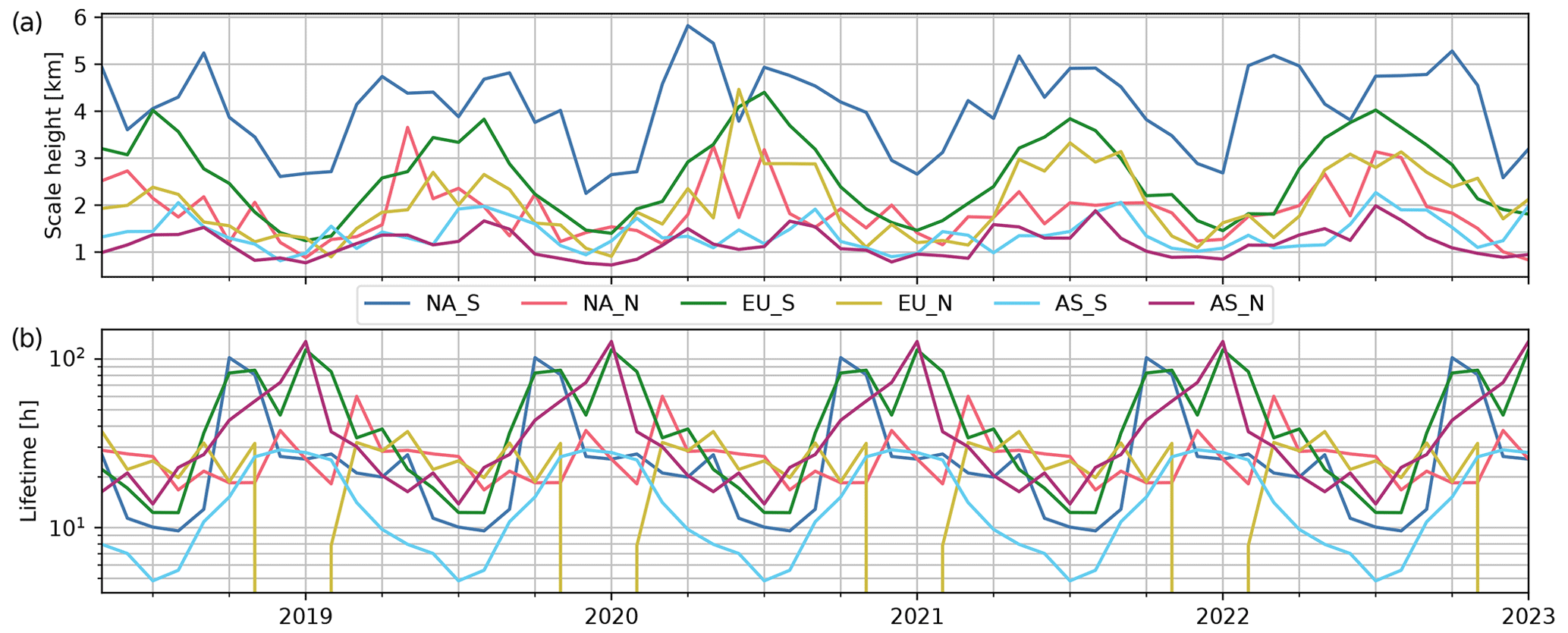
Figure 1 (a) Monthly scale heights fitted using Eq. (2). NA, EU, and AS represent the regions of North America, Europe, and East Asia. S and N after the underscore denote the southern and northern subregions in each region. (b) Chemical lifetimes fitted for these six subregions. Each monthly data point is from the climatology, so all the years have the same seasonality.

Once the monthly NO_x emissions 〈E〉 are obtained using the monthly fitted X and τ, NO_x emissions from each selected city are calculated by averaging NO_x emission grid cells under the geographical coverage of the city (see Sect. 2.2 for the determination of city coverage). The NO_x emission grid cells are weighted by the fraction of urban area coverage during the averaging.

3.3 Algorithms for city clustering based on annual emissions

The monthly NO_x emissions from each city (9 cities per subregion and 54 cities in total) are aggregated annually for cluster analysis in Sect. 4.4. The normalized emissions in 2019–2022 by the 4-year mean are considered the feature for each city and clustered using the k-means clustering algorithm (Likas et al., 2003). The k-means algorithm partitions a set of data points in n-dimensional space (n=4 here, corresponding to annual emissions in 2019–2022) into k clusters, where each data point belongs to the cluster with the nearest mean. The mean or centroid of each cluster is representative of the general pattern of data points in the cluster. A total number of four clusters are used by locating the elbow point of the sum of squared errors as a function of the number of clusters. Additionally, we reduce the feature dimension of four to two using principal component analysis, such that each city can be projected to a two-dimensional scatterplot as shown by Fig. 17.

4 Results

This section dives into the regions in North America, Europe, and East Asia, each with two subregions in the north and south and nine selected cities in each subregion. Section 4.4 synthesizes the annual NO_x emissions from all selected cities through the cluster analysis.

4.1 North America

Figure 2 provides an overview of the region in North America, its two subregions delineated by red rectangles, and selected cities with locations indicated by black arrows. The spatial distributions of NO_x emissions shown by the central map are estimated following Sect. 3.2 in 2019–2022, except that the scale height and chemical lifetime are fitted using the entire region instead of a specific subregion. The southern subregion covers the southwestern USA and northern Mexico, and the northern subregion covers the midwestern and northeastern USA and part of Canada. The annual NO_x emissions in 2019–2022 averaged spatially over each selected city are illustrated as pie charts around the edges of the plot. The sizes of the pies scale with the average city emissions over the 4 years. One may compare the size of slices for 2020–2022 to 2019 as an indication of post-COVID-19 emission changes. Note that the emissions in 2021 and 2022 are generally higher than 2019 for the selected cities in the southern subregion. The slices of 2019 are not larger than one-fourth of the pie in all the cities in the southern subregion: i.e., despite the impacts of COVID-19, the post-COVID annual emissions in these cities are not lower than the pre-COVID year of 2019. The cities in Mexico (Tijuana, Juarez, and Chihuahua) show faster growth of NO_x emissions year to year and stronger emissions compared with neighboring cities in the USA. The northern subregion is quite different in that the NO_x emissions in 2019 are all higher than the 4-year average; i.e., the 2019 slices are larger than one-fourth of the pies. This indicates decreased emissions after COVID-19 that may be attributed to the direct and indirect impacts of pandemic-control measures.

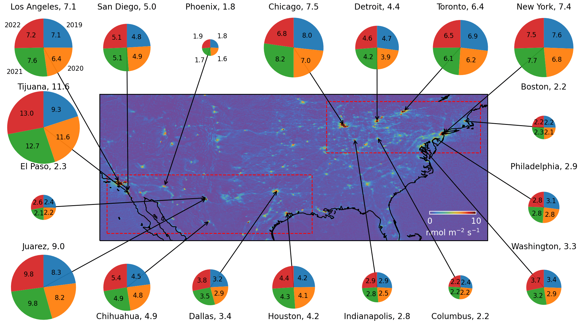
Figure 2 Geographical locations of the 18 cities, 9 in each of the two subregions, in the region of North America. The subregions are outlined by dashed red rectangles. The annual NO_x emissions in 2019–2022 for each city are displayed as pie charts. The emission values for each year are labeled on or near the corresponding slice of the pie ($\mathrm{nmol}{\mathrm{m}}^{-\mathrm{2}}{\mathrm{s}}^{-\mathrm{1}}$). The 4-year average emissions are labeled beside the city names. The central map shows 4-year average NO_x emissions throughout the region. The grid is coarsened from the native size of 0.04 to 0.12^∘ for visualization purposes.

Figures 3 and 4 show the monthly NO_x emissions that are averaged to obtain the annual emissions for cities in the southern and northern subregions in North America (see Fig. 2). In these plots, each city corresponds to one panel, and the panels are ordered by population as provided by the city list (same for all the following nine-panel and one-panel per-city figures). For each panel, the top subpanel shows the absolute monthly NO_x emissions, and the bottom subpanel shows the relative emissions for the same months in 2019. For both subpanels, the values in 2019 are also repeated in the same months for the other years (2018 and 2020–2022) as a baseline for comparison. Higher monthly emissions relative to the same months in 2019 are indicated by red shade, and blue shade is used otherwise. We remove the monthly data with a city-wide average level-2 data coverage lower than 2; i.e., the entire city area has to be on average covered at least twice in the month by TROPOMI observations. This threshold is determined using all the selected cities in this study, and monthly emissions with coverage lower than this value tend to be unreliable. To make consistent interannual comparisons, if one month is removed for a particular year, the same months for all the other years are also removed for a given city. This results in loss of some winter months in high-latitude cities due to high solar zenith angle and snow coverage and wet-season months in some cities due to frequent cloud coverage. Although the monthly emissions are subject to significant variability, NO_x emissions for most cities dropped in early 2020 relative to the same months in 2019, coincident with the initial wave of COVID-19. The relative decrease is more significant in the northern subregion than in the southern subregion. The emissions, relative to 2019, diverge more in 2021 and 2022 among these cities. Some cities in the northeastern USA show comparable or even higher emission reduction in 2022 than in 2020 (e.g., Chicago and Philadelphia), whereas strong growth can be identified in the southern and southwestern USA (e.g., Dallas, Houston, San Diego, and Phoenix) and in Mexico.

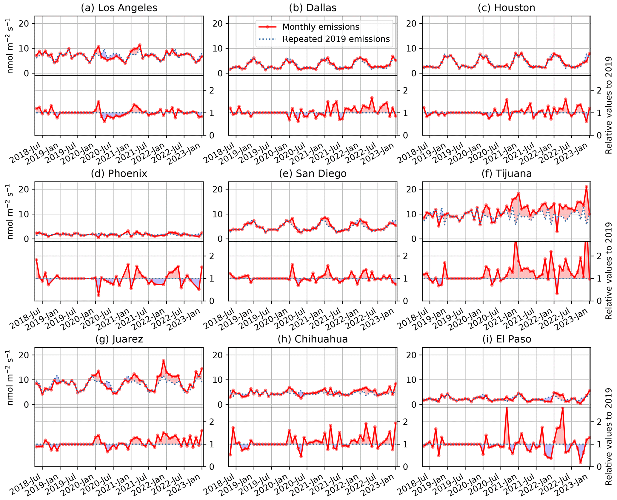
Figure 3 The red dots and lines show monthly NO_x emissions from cities in the southern subregion in North America. For each panel, the top subpanel shows the absolute emissions, and the bottom subpanel shows the relative emissions for the corresponding months in 2019. The blue dashed lines show the 2019 values repeated in the same months for the other years (2018 and 2020–2022). Red and blue shades indicate higher and lower monthly emissions relative to the months in 2019.

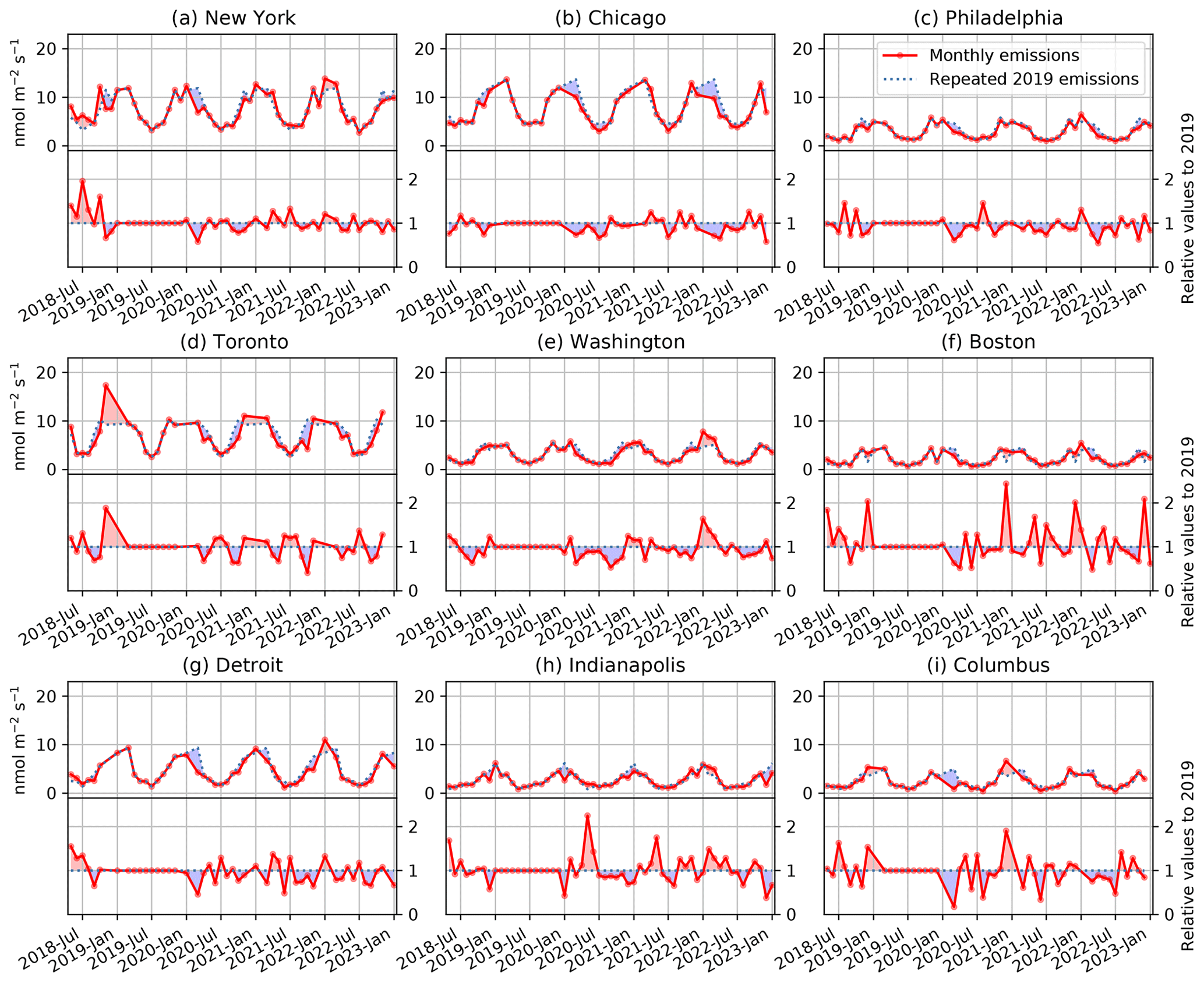
Figure 4 Absolute (top subpanels) and relative (bottom subpanels) monthly NO_x emissions from cities in the northern subregion in North America. This figure is similar to Fig. 3.

Strong seasonal variations with higher emissions in winter months are observed in some cites (e.g., all cities in the northern subregion, Dallas, Houston, San Diego, and Juarez), which is inconsistent with flatter seasonalities often given by bottom-up emission inventories (Sun et al., 2021). These observed seasonal variations might be caused by seasonally varying artifacts, such as retrieval biases, vertical sensitivity of the retrieval at the surface, and the uncertainties in the wind vectors. In addition, because we use a global constant NO_x:NO₂ ratio, its seasonality that is unaccounted for will propagate to the NO_x emission seasonality. One would expect a higher PBL NO_x:NO₂ ratio in winter than summer, but in the summer relatively more NO_x is in the free troposphere, where the NO_x:NO₂ ratio is higher than the PBL (Seinfeld and Pandis, 2016). As a result, the exact impact of the NO_x:NO₂ ratio on each city is inconclusive. However, we note that no clear seasonality can be identified in Tijuana, whereas the adjacent San Diego shows a much more prominent seasonal pattern. This is inconsistent with the potential impacts by the aforementioned factors, because they should have impacted the estimated city emissions similarly at such a close distance. Moreover, similar seasonalities are not as common in the regions of Europe and East Asia to be shown in the following sections. Further validation of the emission values and seasonality will be the subject of future studies.

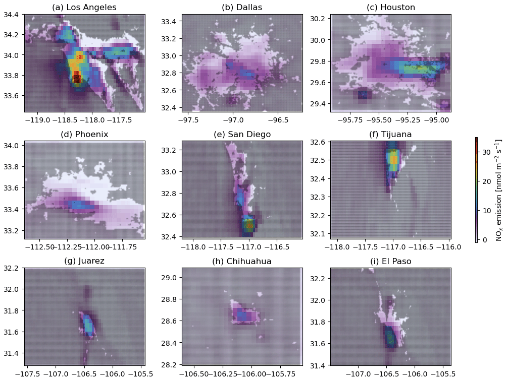
Figure 5 Maps of NO_x emissions and urban area coverage for the nine selected cities in the southern subregion in North America.

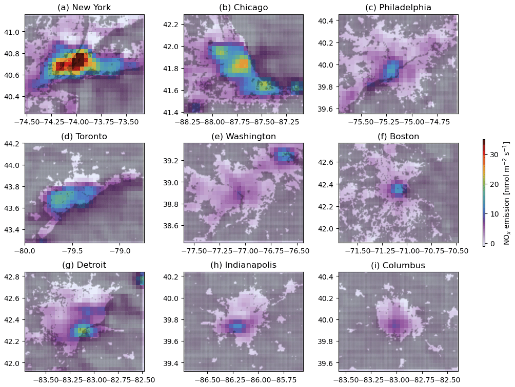
Figure 6 Maps of NO_x emissions and urban area coverage for the nine selected cities in the northern subregion in North America.

The geographical urban area coverage and spatial distribution of NO_x emissions for each city are shown by Fig. 5 (southern subregion) and Fig. 6 (northern subregion). The averaged NO_x emissions in 2019–2022 are displayed at a native grid size of 0.04^∘ as a colored map. The city extent is illustrated as a mask where non-urban area is in black with 95 % transparency, resulting in a gray hue. The city-covered area is fully transparent. The urban sprawl is significant in the USA (Barrington-Leigh and Millard-Ball, 2015), as the city areas in the USA are generally larger than similarly sized cities in other countries. Emission hotspots are often collocated with the downtown areas, but industrial areas and seaports show higher emissions, e.g., the port of Long Beach in Los Angeles (Fig. 5a) and the Houston ship channel (Fig. 5c). The emissions within the city window of Washington, DC, are actually dominated by Baltimore to the northeast (Fig. 6e). Emissions in Tijuana and Juarez are clearly higher than the adjacent American cities San Diego and El Paso, presumably due to different emission regulations.

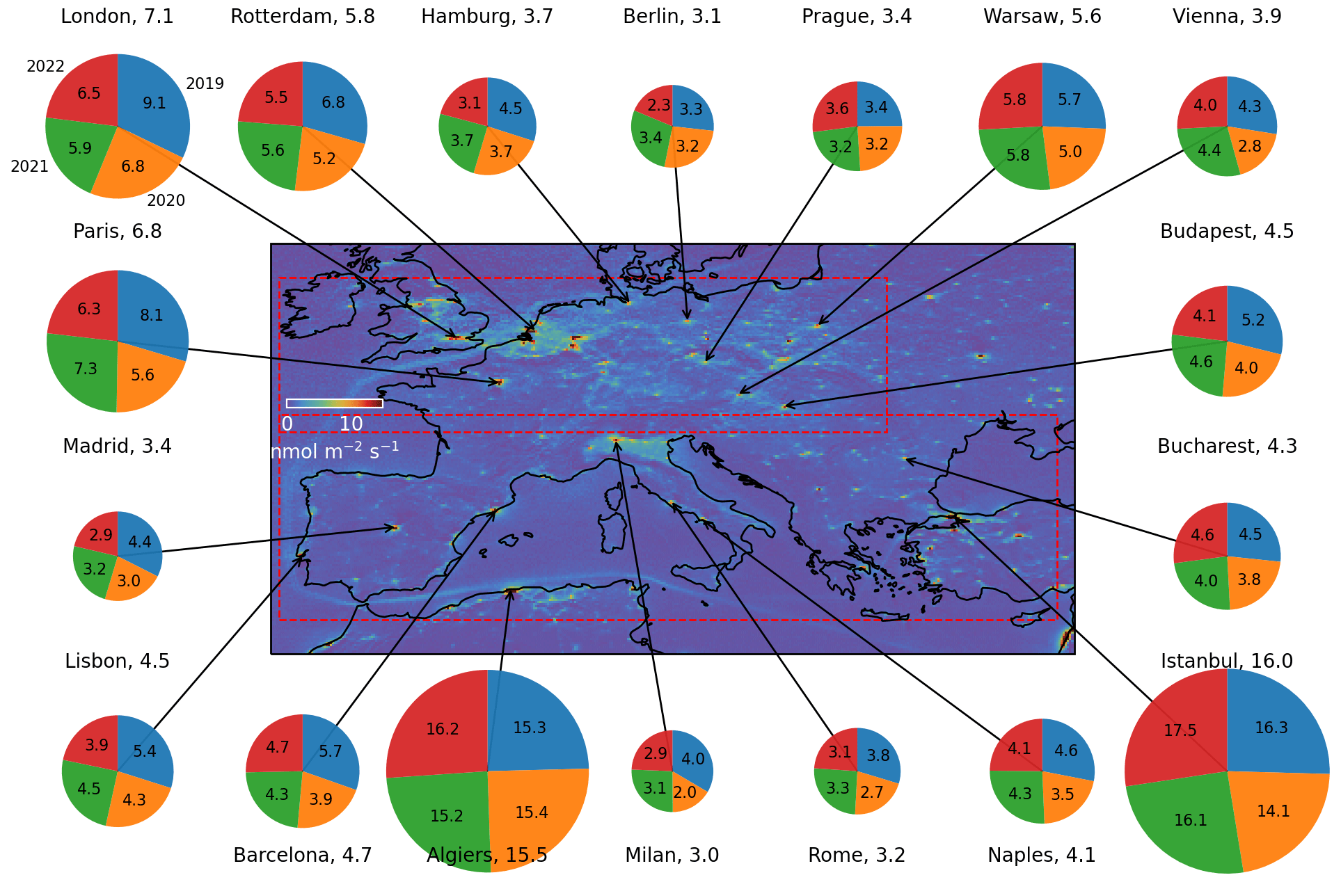
Figure 7 Geographical locations of the 18 cities in the region of Europe. The subregions are outlined by dashed red rectangles. The annual NO_x emissions in 2019–2022 in each city are displayed as pie charts. The emission values for each year are labeled on or near the corresponding slice of the pie ($\mathrm{nmol}{\mathrm{m}}^{-\mathrm{2}}{\mathrm{s}}^{-\mathrm{1}}$). The 4-year average emissions are labeled beside the city names. The central map shows 4-year average NO_x emissions throughout the region. The grid is coarsened from the native size of 0.04 to 0.12^∘ for visualization purposes.

4.2 Europe

Figure 7 is a similar overview for the region of Europe, where the southern and northern subregions are delineated by red dashed rectangles. The NO_x emissions from shipping lanes over the Atlantic Ocean and the Mediterranean Sea are prominent. The annual NO_x emissions in 2019–2022 are shown similarly as pie charts for each city. Note that the southern subregion includes an African city, Algiers in Algeria, due to the rectangular shape of the subregion. Algiers also stands out among other cities in this region in that its 2019 emission is lower than the 4-year average: the 2019 slice is smaller than one-fourth of the pie, and its 2020 emission is higher than 2019. All the other cities show emission reductions in 2020 relative to 2019, which often extend to the following years. Two large cities in developing countries, Algiers and Istanbul, are characterized by larger emissions overall and a stronger rebound of emissions after 2020.

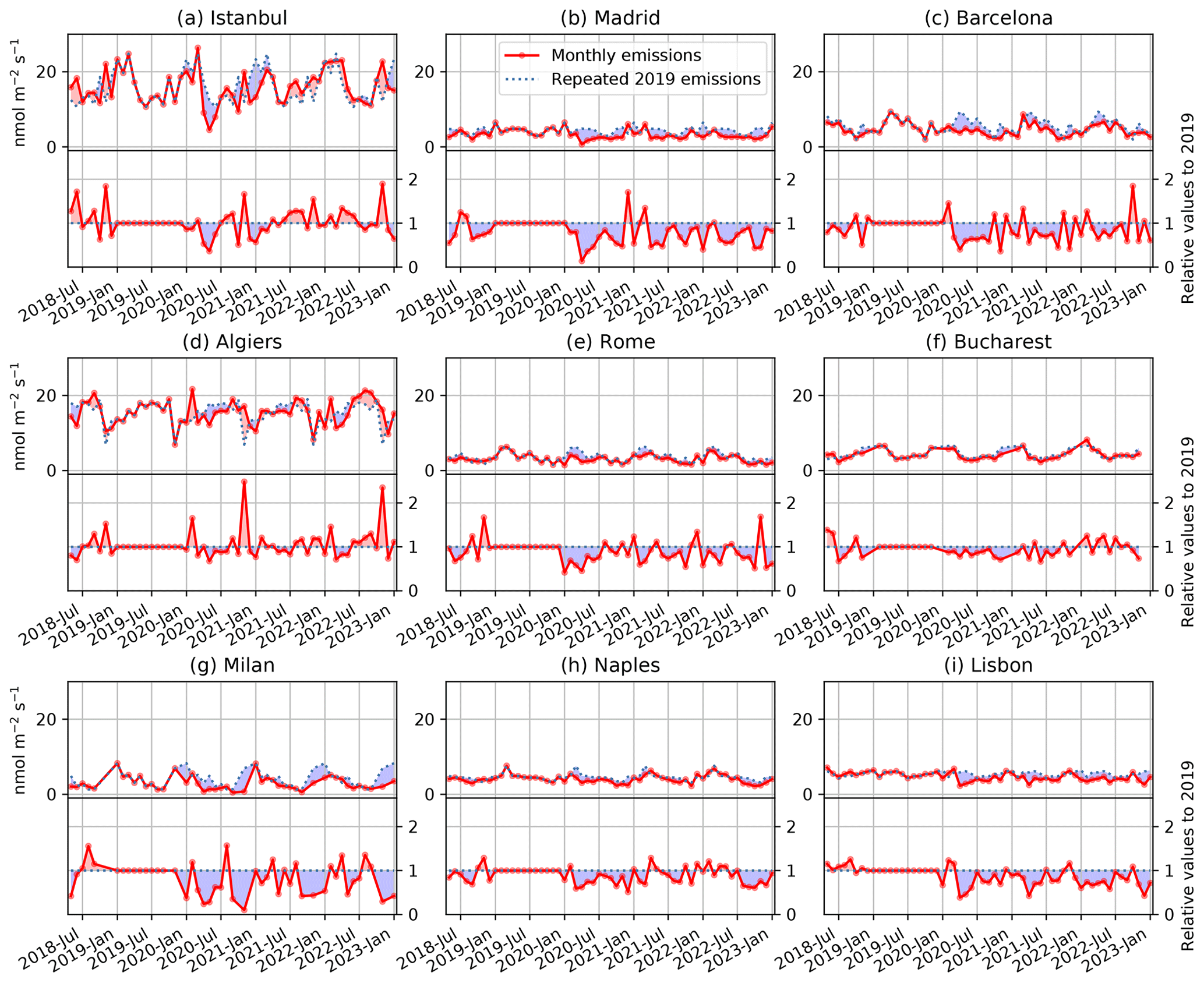
Figure 8 Absolute (top subpanels) and relative (bottom subpanels) monthly NO_x emissions from cities in the southern subregion in Europe. This figure is similar to Fig. 3.

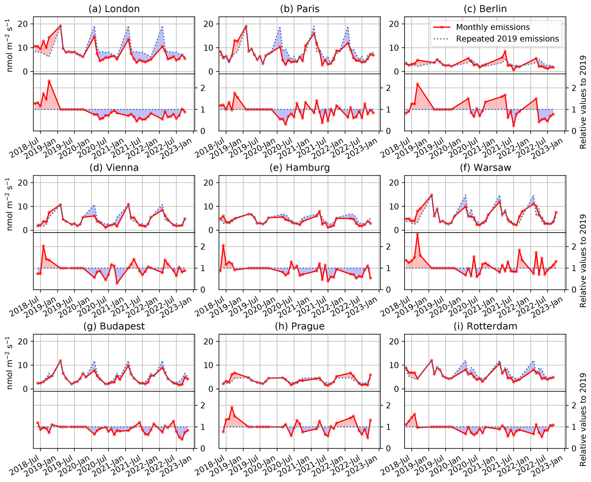
Figure 9 Absolute (top subpanels) and relative (bottom subpanels) monthly NO_x emissions from cities in the northern subregion in Europe. This figure is similar to Fig. 3.

Figures 8 and 9 show the monthly NO_x emissions that are averaged to obtain the annual emissions for cities in the southern and northern subregions in the region of Europe (see Fig. 7). Compared with cities in North America, cities in the European region generally had much larger emission decreases during the initial COVID-19 wave, as indicated by the larger blue-shaded areas. In some cases, most noticeably Madrid, Lisbon, and London, the emission reductions extend almost throughout 2020–2022. Some of the post-COVID-19 reductions relative to 2019 may extend from a pre-existing decreasing trend, as indicated by consistently higher 2018 emissions than 2019 in some cities in the northern subregion (Fig. 9). In contrast, the emissions quickly rebounded after the initial impact in some central and eastern European cities, such as Bucharest, Warsaw, and Prague, as well as in Istanbul and Algiers as mentioned earlier. Some cities in the northern subregion are also subject to significant loss of winter-month coverage due to high solar zenith angle and cloud coverage.

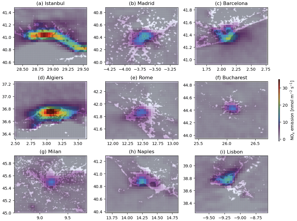
Figure 10 Maps of NO_x emissions and urban area coverage for the nine selected cities in the southern subregion in Europe.

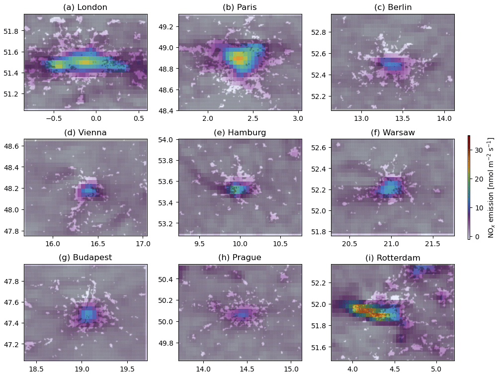
Figure 11 Maps of NO_x emissions and urban area coverage for the nine selected cities in the northern subregion in Europe.

The geographical urban area coverage and spatial distribution of NO_x emissions for each city are shown by Fig. 10 (southern subregion) and Fig. 11 (northern subregion), similar to city maps in the North American region (Figs. 5 and 6). Unlike the American cities that tend to sprawl into a large continuum, the selected European cities tend to be more concentrated, with smaller satellite cities and towns scattered in the surrounding area. The most prominent emission features are generally located at the city centers, with Rotterdam as an exception, where most observed emissions concentrate along the port of Rotterdam, the world's largest seaport outside of East Asia (Fig. 11i).

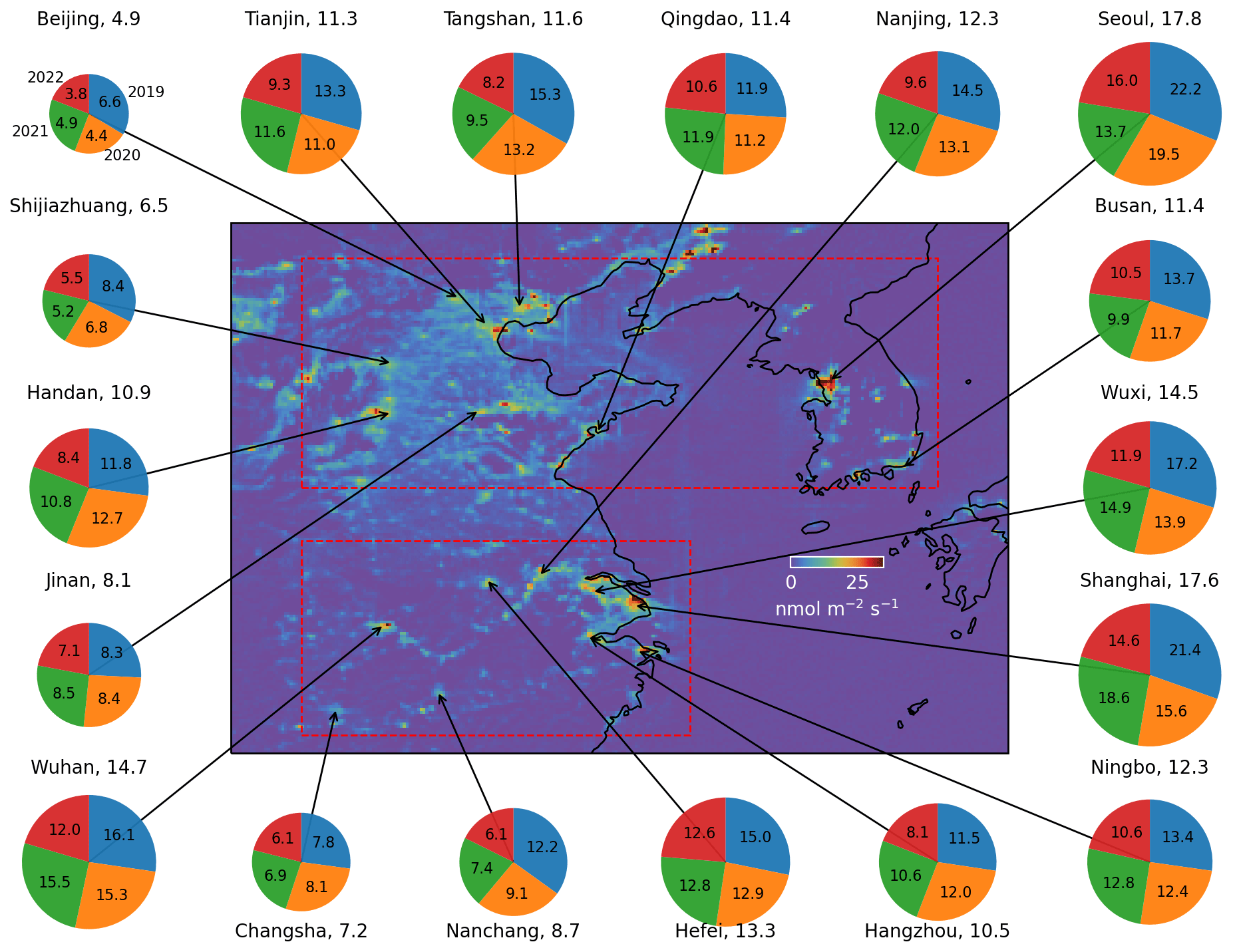
Figure 12 Geographical locations of the 18 cities, 9 in each of the two subregions, in the region of East Asia. The subregions are outlined by dashed red rectangles. The annual NO_x emissions in 2019–2022 in each city are displayed as pie charts. The emission values for each year are labeled on or near the corresponding pie slice ($\mathrm{nmol}{\mathrm{m}}^{-\mathrm{2}}{\mathrm{s}}^{-\mathrm{1}}$). The 4-year average emissions are labeled beside the city names. The central map shows 4-year average NO_x emissions throughout the region. The grid is coarsened from the native size of 0.04 to 0.08^∘ for visualization purposes.

4.3 East Asia

Figure 12 is a similar overview for the region of East Asia, where the southern and northern subregions are delineated by red dashed rectangles. Note that the overall emission background and emissions from individual cities are significantly higher than the regions of North America and Europe, as indicated by the enhanced scale of the color map and pie chart sizes. Selected cities in this region ubiquitously show lower mean annual emissions after COVID-19; i.e., the 2019 pie slices are all larger than one-fourth. Unlike the regions of North America and Europe, the selected cities here all show lower emissions in 2022 than the 4-year average, and in many cases, the 2022 emissions are lower than 2021 and 2020. Out of the 18 selected in this region, 16 are in China, which underwent widespread and stringent measures in 2022 to control the spread of the Omicron variant.

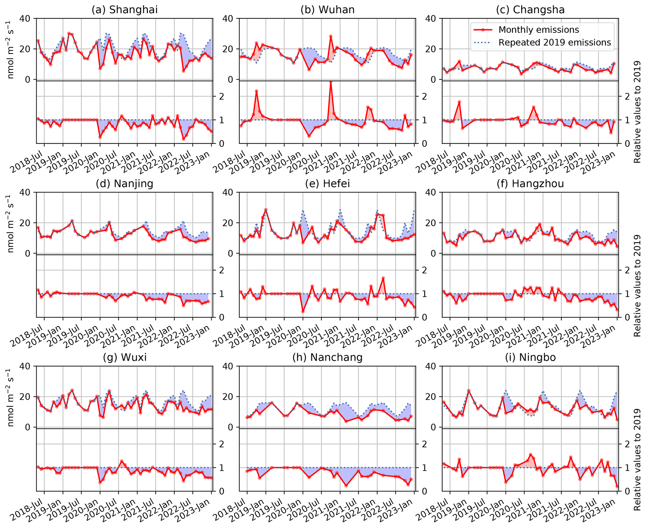
Figure 13 Absolute (top subpanels) and relative (bottom subpanels) monthly NO_x emissions from cities in the southern subregion in East Asia. This figure is similar to Fig. 3.

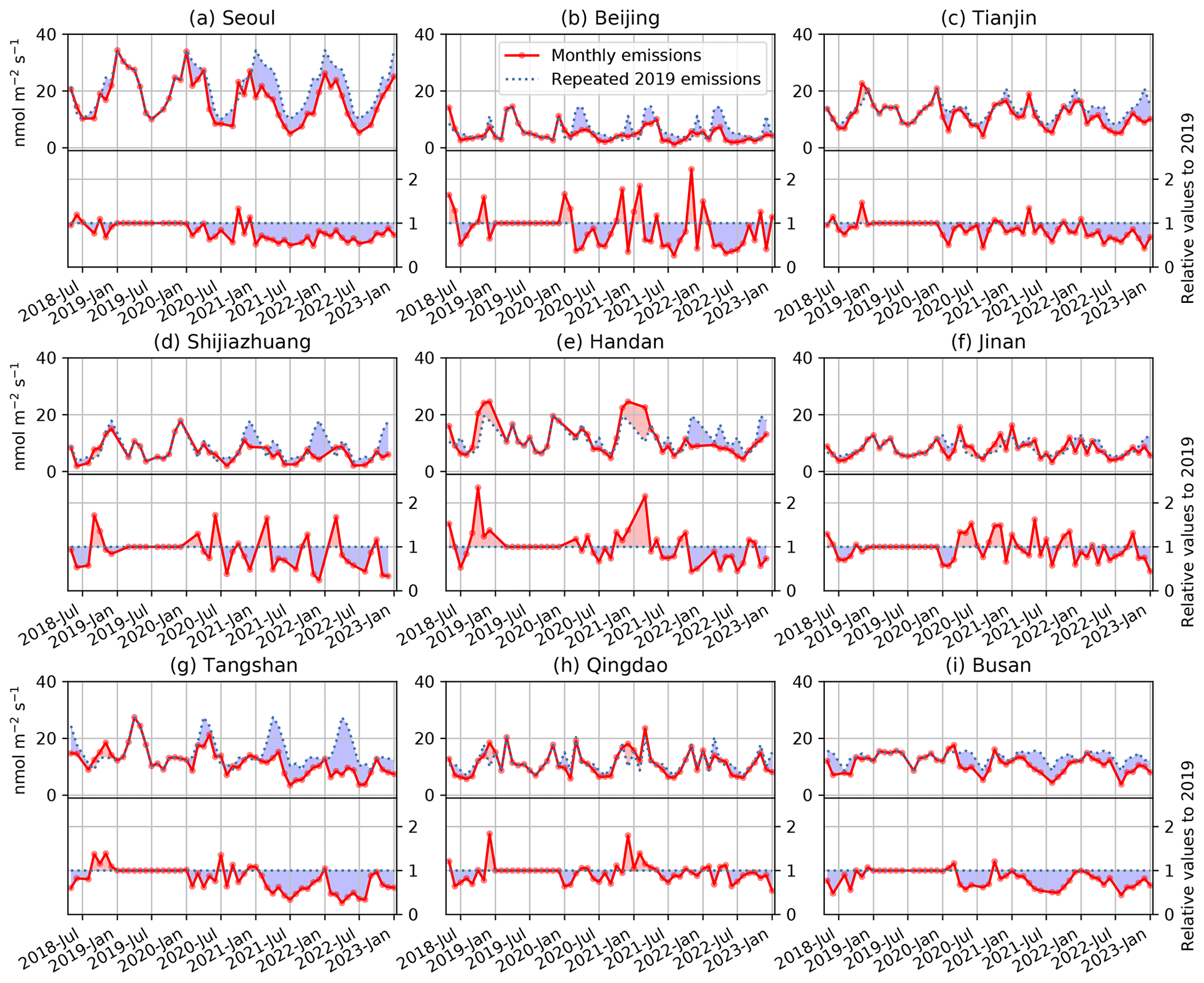
Figure 14 Absolute (top subpanels) and relative (bottom subpanels) monthly NO_x emissions from cities in the northern subregion in East Asia. This figure is similar to Fig. 3.

The temporal evolution of NO_x emissions and their relative changes from 2019 are shown in more detail in the monthly plotted Figs. 13 and 14, with one of the strongest examples of this shown in the megacity of Shanghai in Fig. 13a. Shanghai is one of the largest cities studied here, with higher NO_x emissions than all the other selected cities except Seoul. The data coverage for Shanghai is also complete without any missing months. The well-documented NO_x emission reductions during the spring festival in January and/or February are evident in 2019–2021, although the 2020 spring festival coincided with the initial control measures at the beginning of the COVID-19 outbreak (Liu et al., 2020; Huang and Sun, 2020). Emissions were back to 2019 levels during the second half of 2021. March 2022 marked the start of an unprecedented lockdown in Shanghai in response to the spread of the Omicron variant, and the resultant NO_x emission reductions overshadow those of early 2020. Emission levels largely recovered in August–October 2022 before plunging again due to a nation-wide spread of the Omicron variant, which ultimately led to a termination of most control measures in China in December 2022. The full effect of this policy change on NO_x emissions is not yet clear from the current data.

Figure 13b shows the monthly NO_x emissions in Wuhan, where COVID-19 first drew public attention in January 2020. Data in January and February of all the years are not included due to insufficient TROPOMI coverage, resulting in missing peak lockdown months. Therefore, the relative reduction in 2020 is likely underestimated. Another noteworthy feature in Wuhan is that the October emissions in 2018 and 2020–2022 are all higher than October 2019. One likely cause is the emission reduction measures conducted to ensure good air quality during the 7th Military World Games held in Wuhan in October 2019 (Zhang et al., 2022). As a result, October 2019 emission in Wuhan was likely lower than the business-as-usual condition, leading to spurious enhancements in October of all the other years. The other selected cities similarly show emission reductions in early 2020 during the onset of the pandemic and more extensive reductions in 2022 due to direct and indirect impacts of the Omicron variant spread. Some cities show consecutive months of recovery or increase in emissions in between, e.g., Hangzhou, Ningbo, and Jinan, for the summer and fall of 2020.

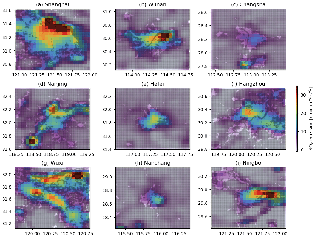
Figure 15 Maps of NO_x emissions and urban area coverage for the nine selected cities in the southern subregion in East Asia.

Similar to the regions of North America and Europe, the geographical urban area coverage and spatial distribution of NO_x emissions for each city in the region of East Asia are shown by Fig. 15 (southern subregion) and Fig. 16 (northern subregion). Unlike most cities in North America and Europe, the strongest emissions in the selected Asian cities are often not located at the city centers but in industrial areas or seaports. Here we try to identify the most prominent emission hotspots on the city maps. The strongest emissions in Shanghai occur in the highly industrialized Baoshan and Pudong districts along the Yangtze River shore (Fig. 15a). For Wuhan, the strongest emissions occur in the district of Qingshan, where Wuhan Iron & Steel is located (Fig. 15b). The emission hotspot in the southwest of Nanjing (Fig. 15d) is the city of Maanshan, home of Maanshan Iron & Steel. The emission hotspot in the northeast of Wuxi (Fig. 15g) is part of Zhangjiagang, a county-level city (in contrast to prefecture-level cities) under the administration of Suzhou. The emission hotspot to the east of Ningbo (Fig. 15i) appears to be part of the port of Ningbo and Zhoushan, the world's largest cargo-handling port.

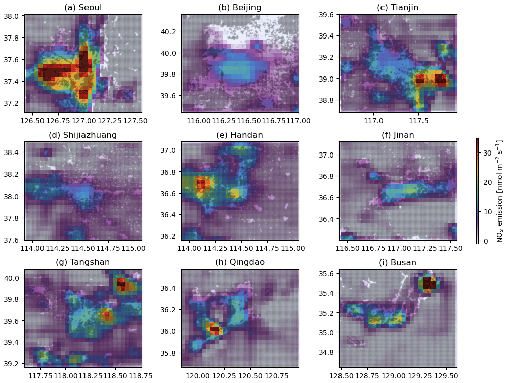
Figure 16 Maps of NO_x emissions and urban area coverage for the nine selected cities in the northern subregion in East Asia.

The city window around Seoul (Fig. 16a) includes most of the Seoul metropolitan area, which was mapped for high-resolution NO₂ column amounts during the Korea–United States Air Quality (KORUS-AQ) campaign (Choo et al., 2023). The west–east extended hotspot in the west of the city window is associated with the Incheon industrial complex, while the more south–north extended hotspot at the center of the city window is located over the city of Seoul. The emission hotspot in the south is located near Suwon, which is also industrialized. The emission hotspot to the southwest of Tianjin (Fig. 16c) collocates with the port of Tianjin, the largest port in northern China and the main maritime gateway to Beijing, and the adjacent industrial area in the Binhai New Area. The emission hotspot to the northeast of Tangshan (Fig. 16g) appears to be Qian'an, a county-level city under the administration of Tangshan, and is the location of Yanshan Iron & Steel. The emission hotspot to the southwest of Qingdao (Fig. 16h) appears to be the port of Qindao. The emission hotspot to the northeast of Busan (Fig. 16i) appears to be the port of Ulsan, the largest industrial port in South Korea.

4.4 Clustering of city emissions

The monthly NO_x emissions calculated for each of the 54 selected cities contain a large amount of information that is challenging to digest. These monthly values are often subject to a low signal-to-noise ratio, especially for the cold-season months in high-latitude cities. As such, we aggregate to annual emissions for the years of 2019–2022 to obtain more insights into how different cities' emissions responded after the onset of COVID-19. For each city, the same months are included for all these years to enhance the interannual consistency. The resultant annual emissions are already shown in Figs. 2, 7, and 12. These annual emissions (four values for each city) are normalized by the 4-year mean and then grouped into four clusters using the k-means algorithm. The normalized annual emission for each city corresponds to a point in the four-dimensional space. To visualize the clustering results, we reduce the dimension of the normalized annual emissions by calculating two principal components, which effectively projects the data to a two-dimensional subspace.

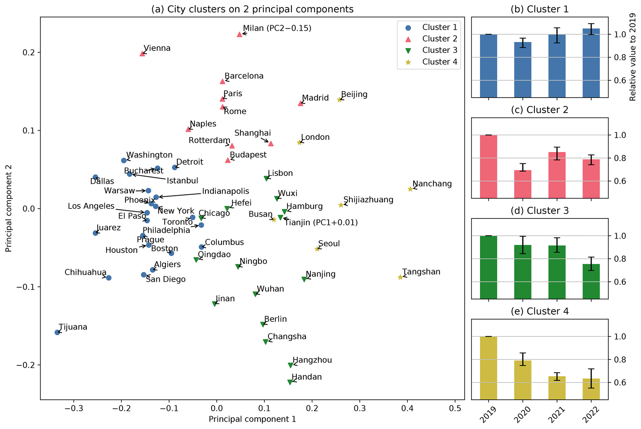
Figure 17 (a) Clustering results using 54 cities selected in this study. The normalized annual emissions in 2019–2022 for each city are projected to two-dimensional space using principal component analysis. The locations of Tianjin and Milan, defined as the two principal components, are nudged downward and right, respectively, to enhance the visualization quality. (b–e) The bars indicate the cluster center, and the error bars indicate the interquartile range within the cluster. The values are all relative to 2019.

Figure 17a shows the distributions of cities in the projected two-dimensional subspace, where each city is a point marked differently according to the cluster it belongs to. The annual emissions for cities in the same cluster are shown as values relative to the 2019 emission in Fig. 17b–e, where the bars indicate the cluster average and the error bars indicate the interquartile range within the cluster. All the cities in the North American region, with Chicago as the only exception, are included in cluster 1 (Fig. 17b), which is characterized by the lowest emission reduction in 2020 (−7 % relative to 2019), with emissions recovering to the 2019 level in 2021 and increased emissions in 2022 (+5 % relative to 2019). Bucharest, Warsaw, Prague, Algiers, and Istanbul in the European region are also included in this cluster. The overall characteristic of cluster 1 is a minor reduction in 2020 relative to 2019 and a steady increase afterwards.

Cluster 2 (Fig. 17c) features the most significant emission reduction in 2020 (−31 % relative to 2019), with a moderate rebound in 2021 (−15 %) and a drop again in 2022 (−21 %). Cities in this cluster are all in the European region, except Shanghai. Cluster 3 (Fig. 17d) differs from cluster 2 in that the emission reduction in 2020 is not as large (−8 %), while the reduction in 2022 is very significant (−25 %), especially in comparison with its value in 2021 (−8.5 %). Cluster 3 mainly includes cities in China, with a few exceptions in Europe (Lisbon, Hamburg, and Berlin) and North America (Chicago). This is consistent with the general evolution pattern of COVID-19 in China: quick recovery of emissions in late 2020 due to effective COVID-19 control measures, sporadic lockdowns in 2021, and much larger-scale lockdowns in 2022.

Cluster 4 (Fig. 17e) is characterized by the largest and sustained decrease in emissions from 2019 to 2022. The average emission reduction in 2022 in this cluster is −37 % relative to 2019, the lowest for all the years in all the clusters. The reduction in 2021 is −35 %, also substantially more than all the other clusters. Cities in this cluster are located in northern China and South Korea, with London as the only exception. Additionally, Tangshan, Seoul, and Busan in cluster 4 have large contributions from industrial NO_x sources (see Fig. 16), suggesting influences from economic factors in addition to direct COVID-19-control impacts.

5 Conclusions and discussion

We apply the directional derivative approach developed by Sun (2022) to estimate NO_x emissions in three Northern Hemisphere regions: North America, Europe, and East Asia. For each region, the NO_x scale heights and chemical lifetimes, which are necessary in the emission calculation, are estimated separately in two subregions. We focus on emissions from 9 selected cities per subregion and present monthly averages and 4-year averaged emission maps at a 0.04^∘ grid size for a total number of 54 cities. The NO_x emission maps reveal unprecedented levels of detail for a large and diverse collection of cities. NO_x emission hotspots are consistently found at large city cores, while some cities feature significantly higher emissions than others, most notably at the USA–Mexico border (San Diego vs. Tijuana and El Paso vs. Juarez). The spatial windows of some cities encompass much more prominent emission hotspots than the city cores, which generally correspond to large seaports and industrial areas. The average emissions in 2019–2022 are generally larger in East Asian cities, as 13 out of 18 cities in this region are higher than 10 $\mathrm{nmol}{\mathrm{m}}^{-\mathrm{2}}{\mathrm{s}}^{-\mathrm{1}}$. In contrast, only one city in the North American region (Tijuana) and two cities in the European region (Algiers and Istanbul) are higher than this value.

With respect to the temporal variation of NO_x emissions, we choose the year of 2019 as the pre-COVID-19 baseline year, so the relative emission changes in 2020–2022 to 2019 indicate the post-COVID-19 perturbations to each city. We caution that the relative differences between the post-COVID-19 months in 2020–2023 and the corresponding months in 2019 may exist even without COVID-19. These non-COVID-19 factors include the Military World Games impact in Wuhan and a pre-existing long-term decreasing trend in many cities in the northern European subregion, as indicated by the higher emission in 2018 than 2019 (Fig. 9). The initial impact during the first outbreak of COVID-19 in early 2020 can be found in most cities, but their paths diverge afterwards. We average the monthly emissions for each city to annual mean emissions in 2019–2022 and group the normalized annual mean emissions into four clusters. All but one city in the North American region are grouped in cluster 1, which is characterized by the smallest emission reduction in 2020 (−7 %) and a steady increase afterwards, resulting in a +5 % increase in 2022. Limited representations of Latin America (Tijuana, Juarez, and Chihuahua), Africa (Algiers), and the Middle East (Istanbul) are all located in cluster 1. Future studies might be meaningful for testing whether the emission-changing pattern of cluster 1 is common in these regions. The other clusters (2–4) feature much larger emission reductions than cluster 1 and differ by how these reductions are distributed in 2020–2022. The European cities are generally in cluster 2, with the largest impact in 2020 (−31 %), whereas the East Asian cities are generally in clusters 3 and 4, with the largest impacts in 2022 (−25 % and −37 %).

In this study, we fit scale heights at monthly resolution and fit chemical lifetimes for each climatological month to strike a balance between the quality of the fitting results and the temporal resolution. However, we assume spatially homogeneous scale heights and chemical lifetimes within each subregion. Considering that the fitting is conducted over cleaner locations where the free tropospheric NO₂ subcolumn is expected to take a larger fraction of the tropospheric column, the fitted scale heights and chemical lifetimes are likely overestimated for urban areas. Additionally, the NO_x chemical lifetime is highly nonlinear with respect to the NO_x concentration (Valin et al., 2013; Laughner and Cohen, 2019). Therefore, although some aspects of the fitted results are consistent with the expected spatial and temporal variation of the PBL height and NO_x chemical lifetime, we caution that the inverses of scale heights and chemical lifetimes are fundamentally linear fitting parameters and caution against over-interpretation of the results. Future investigations might be helpful for achieving higher spatial granularity and/or considering the dependencies of scale height and chemical lifetime on the column amount. We choose a constant NO_x:NO₂ ratio, given the emphasis of this study on relative emission changes and the timeliness of emission estimation. An improved understanding of the global NO_x:NO₂ ratio over the atmospheric columns through which satellite sensors integrate will likely enhance the quality of estimated NO_x emissions.

This work presents observation-based NO_x emission estimations over large areas (covering three major continents), with fine spatial resolution (0.04^∘, resolving intracity emission variations), high temporal resolution (monthly), and timely results (until 31 January 2023). The main focus of this work is the relative emission changes for each city in the pre- and post-COVID-19 years. The absolute emission values of one city compared with another and absolute estimates of emissions month by month would be subject to larger uncertainties than the relative values, given the assumptions and simplifications discussed above. We expect future evaluations of spatiotemporal variations of derived emissions against known emission rates of point sources and bottom-up emission inventories. The current workflow requires only TROPOMI level-2 data and the ERA5 reanalysis, both publicly available with global coverage, and the open-source Python algorithm (Sun, 2023). It is our hope that this tool will benefit future studies that cover more regions in the world and use additional remote-sensing instruments.

Appendix A: Key assumptions in flux divergence vs. the directional derivative approach

The flux divergence approach (e.g., Beirle et al., 2019, 2021; de Foy and Schauer, 2022; Dix et al., 2022) is based on the following equation, expressed in terms defined in this work.

$$\begin{array}{ll}{\displaystyle }\langle E\rangle & {\displaystyle }=\langle \mathrm{\nabla }\cdot \left(\mathrm{\Omega }\mathit{u}\right)\rangle +{\displaystyle \frac{\langle \mathrm{\Omega }\rangle }{\mathit{\tau }}}\\ \text{(A1)}& {\displaystyle }& {\displaystyle }=\langle \mathit{u}\cdot \left(\mathrm{\nabla }\mathrm{\Omega }\right)\rangle +\langle \mathrm{\Omega }(\mathrm{\nabla }\cdot \mathit{u})\rangle +{\displaystyle \frac{\langle \mathrm{\Omega }\rangle }{\mathit{\tau }}}\end{array}$$

Here the second step makes it clearer to compare with the counterpart of the directional derivative approach (i.e., Eq. 1). The key implicit assumptions of the flux divergence approach are discussed below.

1. The emission includes the divergence of horizontal flux and chemical loss. Without the chemical loss, the emission equals the horizontal flux divergence, as shown by studies applying flux divergence to methane (Liu et al., 2021; Veefkind et al., 2023). The problem is that the divergence of horizontal flux is also driven by the divergence of wind (∇⋅u), which can have positive or negative values climatologically for different locations. This leads to spurious emission values seen in the flux divergence literature that often need empirical correction (Liu et al., 2021; Dix et al., 2022; Veefkind et al., 2023).

2. The topography does not contribute to the flux divergence. In reality, the wind vector usually partially aligns with the gradient of surface altitude even over a long-term average, resulting in terrain-dependent artifacts.

The directional derivative approach (Sun, 2022, this work) addresses these assumptions by explicitly considering the wind divergence and topography effects. The assumptions that lead to the directional derivative approach are detailed in Sun (2022) and discussed below.

1. There exists an altitude z₁ where emissions, as observed by satellites, are confined within. We equate z₁ as the PBL height for ease of conceptualization, but it does not have to be explicitly defined to derive Eq. (1).

2. The horizontal gradient of subcolumn amounts above z₁ is negligible compared with that below z₁ at the spatial scale of adjacent satellite observations.

3. The vertical flux of observed species at z₁ is only due to divergence or convergence of wind below z₁ and is thus not sensitive to emissions. This assumption is a consequence of assumption 1 and the assumption that air flow is incompressible.

4. The scale height of the observed species is a constant through the domain. This is necessary for relating the surface concentration to the column amount in the topography term.

5. The column-integrated chemical lifetime of the observed species is a constant through the domain. This is necessary to simplify the chemical loss term, and it is the same for the flux divergence approach.

Assumptions 1–3 are from reasoning. We encourage future testing of these assumptions, presumably through high-quality model simulations. Assumptions 4–5 are apparently significant simplifications. The following two paragraphs discuss their implications.

The scale height is expected to be lower over polluted regions than clean regions. We fit the scale height over rough terrains in each subregion, which are inherently cleaner than the urban areas. Therefore, the scale height applied to urban areas is likely overestimated, and the topography term is hence underestimated as it scales with the inverse of scale height. Fortuitously, the urban areas are generally situated over flat terrains. The median value of the monthly term $|\langle \mathrm{\Omega }{\mathit{u}}_{\mathbf{0}}\cdot (\mathrm{\nabla }{z}_{\mathrm{0}})\rangle |$ for all 54 cities averaged in each city is 1.3 × 10⁻⁷ $\mathrm{mol}{\mathrm{m}}^{-\mathrm{1}}{\mathrm{s}}^{-\mathrm{1}}$. This means that neglecting the topography effect resulting from a 1000 m scale height would only give rise to an emission error of 1.3 × 10⁻¹⁰ $\mathrm{mol}{\mathrm{m}}^{-\mathrm{2}}{\mathrm{s}}^{-\mathrm{1}}$, which is below the noise floor. However, there are two caveats. First, this does not mean that the topography term is unimportant. It might be small over the flat city, but it is large over rough terrains that are close to many cities. Second, some emission sources do appear over rough terrains.

The column-integrated chemical lifetime is a complicated and challenging parameter to obtain. A wide range of values and strategies exists in the literature. Two main factors determine its value: the chemical lifetime within the PBL and the partition of column amounts in the PBL vs. in the free troposphere. The PBL chemical lifetime is highly nonlinear. In the “NO_x-limited” regime, it decreases with increasing NO_x, whereas in the “NO_x-suppressed” regime, the relationship is reversed. The range of variation is within a factor of 2 (Valin et al., 2013; Laughner and Cohen, 2019). The PBL vs. free troposphere partition may have a larger impact given the high urban–rural column amount contrast and the significant free tropospheric contribution in the clean regions (Silvern et al., 2019). Overall, we expect the column-integrated lifetime determined over relatively clean regions to be higher than the true value over urban areas. This is also consistent with the longer lifetimes shown by Fig. 1 than literature values of the urban PBL NO_x lifetime. Consequently, the chemical loss term is likely underestimated in polluted regions.

As such, both topography and chemical loss terms are expected to be underestimated for NO_x over urban areas. This undercorrection is preferred to overcorrection. Directions of future improvements include using model simulations to inform the spatiotemporal variations of scale height and lifetime and fitting more complex functions (e.g., as polynomial functions of the column amount) of the scale height and lifetime. The current constant scale height and lifetime are just the special case of a zeroth-order polynomial. This will require an even higher signal-to-noise ratio, more observations, and/or a finer spatial resolution than TROPOMI.

Appendix B: Comparisons between this work and its precursors

Beirle et al. (2019)Beirle et al. (2021)Dix et al. (2022)de Foy and Schauer (2022)Goldberg et al. (2022)Chen et al. (2023)Sun (2022)

Table B1 Considerations of physical and chemical processes by this work and previous studies. The flux divergence and directional derivative approaches are distinguished by whether wind divergence is included or excluded.

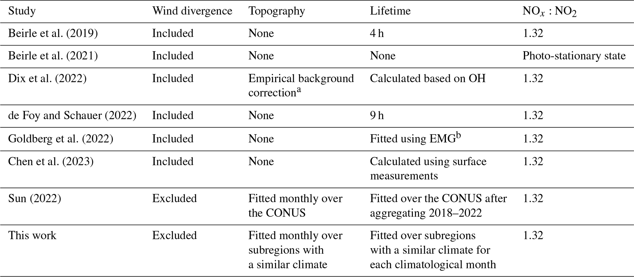
^a This may compensate for both topography and chemical loss effects. ^b EMG: exponentially modified Gaussian function.