Better-constrained climate sensitivity when accounting for dataset dependency on pattern effect estimates

The best estimate of equilibrium climate sensitivity (ECS) constrained based on the instrumental record of historical warming becomes coherent with other lines of evidence when the dependence of radiative feedback on the pattern of surface temperature change (pattern effect) is incorporated. Pattern effect strength is usually estimated with atmosphere-only model simulations forced with observed historical sea-surface temperature (SST) and sea-ice change and constant pre-industrial forcing. However, recent studies indicate that pattern effect estimates depend on the choice of SST boundary condition dataset, due to differences in the measurement sources and the techniques used to merge and construct them. Here, we systematically explore this dataset dependency by applying seven different observed SST datasets to the MPI-ESM1.2-LR model covering 1871–2017. We find that the pattern effect ranges from $-\mathrm{0.01}\pm \mathrm{0.09}$ to 0.42±0.10 W m⁻² K⁻¹ (standard error), whereby the commonly used Atmospheric Model Intercomparison Project II (AMIPII) dataset produces by far the largest estimate. When accounting for the generally weaker pattern effect in MPI-ESM1.2-LR compared to other models, as well as dataset dependency and intermodel spread, we obtain a combined pattern effect estimate of 0.37 W m⁻² K⁻¹ [−0.14 to 0.88 W m⁻² K⁻¹] (5th–95th percentiles) and a resulting instrumental record ECS estimate of 3.2 K [1.8 to 11.0 K], which as a result of the weaker pattern effect is slightly lower and better constrained than in previous studies.

1 Introduction

Governments around the world are putting in extensive efforts to achieve the targets set in the Paris Agreement (2015), where the long-term goals are to limit the increase in global mean temperature to well below 2 ^∘C and pursuing efforts to limit the warming to 1.5 ^∘C above pre-industrial levels. However, the latest Intergovernmental Panel on Climate Change (IPCC, 2021) reported that our planet has already warmed by more than 1 ^∘C relative to pre-industrial levels and that it is likely that we might miss the 1.5 ^∘C target. To know what is required to meet the Paris Agreement goal, it is imperative to better quantify and understand the ultimate amount of warming in response to a given forcing. Equilibrium climate sensitivity (ECS), defined as the long-term warming resulting from a doubling of CO₂ concentration over pre-industrial levels, is a metric of central importance in the quest to constrain projections of future global warming (Grose et al., 2018; Sherwood et al., 2020; Forster et al., 2021). Transient climate response (TCR) is another metric that is often used to study climate change, which is however closely related to ECS (Huusko et al., 2021). Here, we investigate ECS constrained based on the instrumental record of historical warming including corrections for the effects on the radiation balance caused by the pattern of surface temperature change. Relative to earlier studies, we will do so by also accounting for uncertainty and biases caused by the underlying sea-surface temperature (SST) reconstructions used in estimates of the pattern effect.

2 How historical warming is used to constrain ECS

A linear energy budget framework incorporating global mean parameters is widely used to understand the response of the climate system to external perturbations such as a change in atmospheric composition (e.g., Gregory et al., 2002; Otto et al., 2013). It can be framed as $N=F+\mathit{\lambda }T$, where N is the planetary energy imbalance, which is generally defined as the change in net downward radiative flux at the top of the atmosphere (TOA), F is the external radiative forcing, defined as effective radiative forcing (ERF; Hansen et al., 2005; Forster et al., 2021) and T is the change in surface temperature, all relative to an unperturbed equilibrium climate state where $N=F=\mathrm{0}$. λ is the climate feedback parameter which mediates how rapidly the climate system would get rid of the energy imbalance due to the external perturbation. ECS is related to the feedback parameter as ECS = $-F_{\mathrm{2}\times }/\mathit{\lambda }$, where F_2× is the forcing due to a doubled CO₂ concentration, such that

$$\begin{array}{}\text{(1)}& \mathrm{ECS}\approx {\displaystyle \frac{F_{\mathrm{2}\times }\mathrm{\Delta }T}{\mathrm{\Delta }F-\mathrm{\Delta }N}},\end{array}$$

where the change in temperature, forcing and energy imbalance is taken between two periods, e.g., 1850–1900 and 2006–2019 denoted by ΔF, ΔT and ΔN.

Early best estimates of ECS based on the instrumental temperature record (Forster, 2016) are usually found to be at the lower end of the commonly accepted ECS likely range and triggered a lowering of the lower bound between the IPCC's Fourth and Fifth Assessment Reports. For instance, the best estimate of Otto et al. (2013) of the historical energy budget-constrained ECS is 2 K, whereas Lewis and Curry (2015) found a best estimate of 1.64 K. To reconcile this discrepancy, among other things the community looked into the concept of the pattern effect, which is not taken into account in the traditional energy balance framework. The rationale is that if the pattern of temperature response in the historical period is different in ways that affect the radiation balance from what it would be in the future, then constraining ECS based on the instrumental record could be biased. In addition, there has been upward revisions to the temperature record through infilling (e.g., Clarke and Richardson, 2021), downward revisions to total forcing and small revisions to estimates of energy imbalance (Bellouin et al., 2020; Von Schuckmann et al., 2020; IPCC, 2021).

Indeed, it has been identified that inference of λ based on the instrumental record not only relies on the global mean temperature but also on its spatial structure (Armour, 2017; Andrews et al., 2018; Lewis and Mauritsen, 2021; Fueglistaler and Silvers, 2021). Different patterns of temperature response lead to different circulation and cloud response. This in turn impacts the energy budget and hence could induce dissimilar λ (Zhou et al., 2016; Mauritsen, 2016; Ceppi et al., 2017). The dependence of the radiative feedback on the spatial pattern of temperature response is referred to as the “pattern effect” (Stevens et al., 2016).

Whereas a colder tropical eastern Pacific and Southern Ocean (SO) and stronger tropical western Pacific warming are observed over the historical period, atmosphere–ocean general circulation models (AOGCMs) simulate a long-term climate response (to abrupt4×CO₂) that resembles a temperature pattern similar to the El Niño–Southern Oscillation (ENSO) with relatively larger warming trends in the eastern Pacific and SO (Andrews et al., 2015; Zhou et al., 2016; Dong et al., 2019; Sherwood et al., 2020; Watanabe et al., 2021). This difference in the distribution of temperature response induces a pattern effect since a warmer west Pacific and colder east Pacific lead to more stabilizing feedback, while the simulated future temperature distribution would lead to a less stabilizing feedback (Zhou et al., 2016; Mauritsen, 2016; Ceppi et al., 2017; Andrews and Webb, 2018; IPCC, 2021).

The strength of the pattern effect can be estimated as the difference in the radiative feedback obtained from a historical climate change simulation from that obtained from a long-term response simulation such as abrupt4×CO₂ (Fig. 1, Armour, 2017; Andrews et al., 2018; Lewis and Mauritsen, 2021). One approach to determine an observationally constrained historical pattern effect is to prescribe the observed historical SST and sea-ice evolution such as the Atmospheric Model Intercomparison Project II (AMIPII) dataset to the atmosphere general circulation models (AGCMs) as a boundary condition with pre-industrial forcing (Andrews et al., 2018). This observedSST-piForcing configuration in principle simulates a TOA energy imbalance following the historical SST pattern evolution and hence facilitates the computation of historical λ for the given model and dataset (Figs. 1 and A1). Such estimates are model dependent; nevertheless most models yield a dampening pattern effect relative to the long-term abrupt4×CO₂ pattern based on the AMIPII dataset (e.g., Andrews et al., 2018).

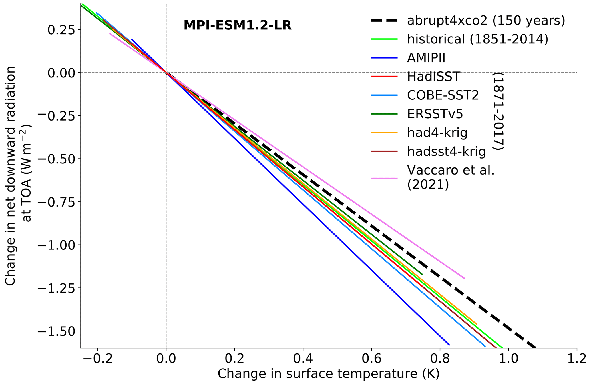
Figure 1 Linear fits from ordinary least squares (OLS) regression between the change in global annual mean net downward radiation flux at the TOA and the surface temperature change (Gregory et al., 2004) for different AOGCM (abrupt4×CO₂, historical) and observedSST-piForcing atmosphere-only GCM simulations (named per dataset, shown in legend). The global annual mean values are not shown but only the regression fits. The changes are relative to the 1871–1900 mean. The y intercept is adjusted such that all linear fits begin from the origin. The pattern effect (Δλ) is the difference between the regression fits (solid lines) and the abrupt4×CO₂ fit (dashed line). See Fig. A1, which shows the global annual mean values with OLS regression.

However, this approach to estimating the pattern effect relies on the observed–reconstructed SST datasets applied to the AGCMs as boundary conditions, and hence the estimates of the pattern effect derived from such modeling experiments might depend on the applied SST dataset. Only a few studies (Lewis and Mauritsen, 2021; Fueglistaler and Silvers, 2021; Andrews et al., 2022) have addressed the dataset dependency of the pattern effect in limited setups. Lewis and Mauritsen (2021) compared only two datasets, AMIPII and HadISST, although they assessed the pattern effects derived using the Green's function approach with six other reconstructed datasets. They concluded that using alternative datasets yields a smaller pattern effect similar to that simulated by coupled climate models running the historical scenario. Fueglistaler and Silvers (2021), on the other hand, did not conduct simulations but instead based on temperature metrics that rely on the region of deep convection and tropical average SSTs, a proxy for pattern effect (Dong et al., 2019), showed that AMIPII stands out from the rest of the considered datasets.

In this study, we address this problem by applying seven datasets covering 1871–2017 to the MPI-ESM1.2-LR model. We simulate a range of pattern effect estimates based on the datasets. The resulting dataset-dependent estimates of the pattern effect is then extended to include model dependency estimated by Andrews et al. (2022) in order to update the ECS estimates constrained by the instrumental record reported in Forster et al. (2021).

3 Model, datasets and experiments

The MPI-ESM1.2-LR climate model (Mauritsen et al., 2019) was part of the Coupled Model Intercomparison Project Phase 6 (CMIP6). The atmosphere model component is ECHAM6.3. Through surface exchange of mass, momentum and heat, it is coupled to the land model JSBACH3.2. The horizontal resolution is spectral T63, corresponding to approximately 200 km grid spacing, while there are 47 hybrid-sigma pressure levels in the vertical. We configure MPI-ESM1.2-LR to run in atmosphere-only mode where the SST boundary conditions are prescribed based on the observed historical surface temperature evolution.

The seven different observed–reconstructed SST datasets applied as boundary conditions are HadISST1 (Rayner et al., 2003), AMIPII (Hurrell et al., 2008), COBE-SST2 (Hirahara et al., 2014), ERSSTv5 (Huang et al., 2017), had4_krig and had4sst4_krig (Cowtan and Way, 2014) and Vaccaro2021 (Vaccaro et al., 2021a; Table A1). All of these datasets are globally complete, infilled fields of SST at a monthly resolution from 1871 to 2017. The had4krig, had4sst4krig and Vaccaro2021 datasets are available only as anomalies relative to a base period. We have used the corresponding base period from COBE-SST2 to create the absolute temperatures. The differences among these datasets arise from the differences in the (1) measurement sources that they are constructed from, the bulk of which is common, (2) assimilation and bias correction methods applied and (3) infilling methods employed which aim to construct a spatially complete dataset. For instance, had4krig and had4sst4krig employs an optimal interpolation algorithm known as kriging (Cressie, 1990) to HadCRUT4 data, whereas Vaccaro2021 employs a method based on Gaussian graphical models applied to the raw HadCRUT4.6 (Vaccaro et al., 2021a). A comparison of the dataset properties is given in Table A1.

The datasets are regridded to the Gaussian grid corresponding to the T63 resolution of MPI-ESM1.2-LR. We performed a bi-linear interpolation on the datasets. The same is done for the AMIPII sea-ice data which is set as the boundary condition for sea-ice concentration in all the simulations in order to isolate the effect of the SSTs. We apply pre-industrial forcing to these set of simulations and named them observedSST-piForcing. We perform an ensemble of five observedSST-piForcing simulations for each dataset. Unless otherwise specified, throughout the text, the displayed results are based on the mean of the five ensemble simulations while the uncertainty denotes the standard error from the ordinary least squares (OLS) regression and the ranges are the 5th–95th percentiles.

As expected, the historical evolution of the global annual mean surface temperature anomaly from the observedSST-piForcing simulations are similar (Fig. 2a). The differences are due to differences in the way the SST fields are reconstructed and partly due to land surface warming, which evolves on its own in these simulations. The temperature anomaly in the ERSSTv5-forced observedSST-piForcing simulation is lower compared to others, consistent with Fueglistaler and Silvers (2021). This is related to ship SST bias corrections made to temperature during the 1880s–1940s and 1950s–1960s (Huang et al., 2017; Fig. 2a).

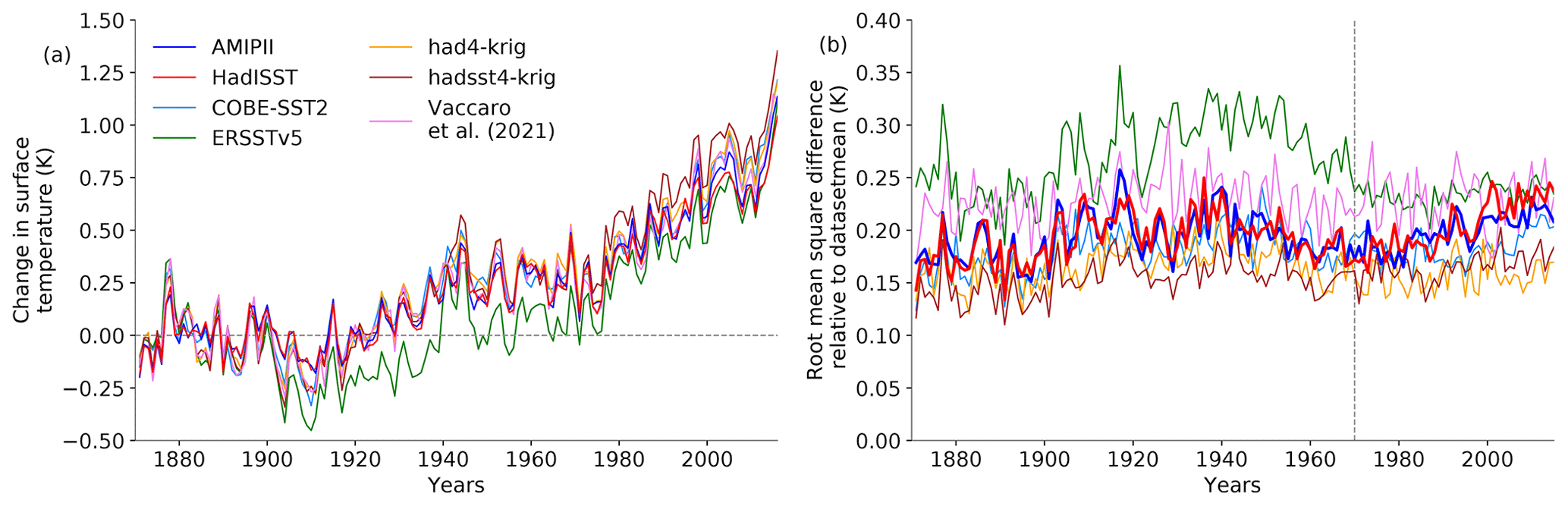
Figure 2 Evolution of simulated global mean surface temperature anomaly (a) and root-mean-square deviation (RMSD) of the temperature anomaly for the seven observedSST-piForcing simulations relative to the dataset mean (b). The dashed gray line in (b) marks the year 1970. The RMSD are calculated over each ocean grid with the land masked. The temperature anomalies are relative to the 1871–1900 mean.

The root-mean-square deviation (RMSD) of the surface temperature anomaly between the individual observedSST-piForcing simulations and their mean diverges most in the case of ERSSTv5 until the 1970s (Fig. 2b–d), which is probably mostly due to the lower global mean warming in that dataset. The differences reduces to within 0.15 K after the 1970s. Although there is a close agreement in the global mean evolution of surface warming, we find apparent regional differences in the temperature anomaly trends shown in Fig. 3. These differences in the pattern of surface temperature change could lead to different estimates of the pattern effect.

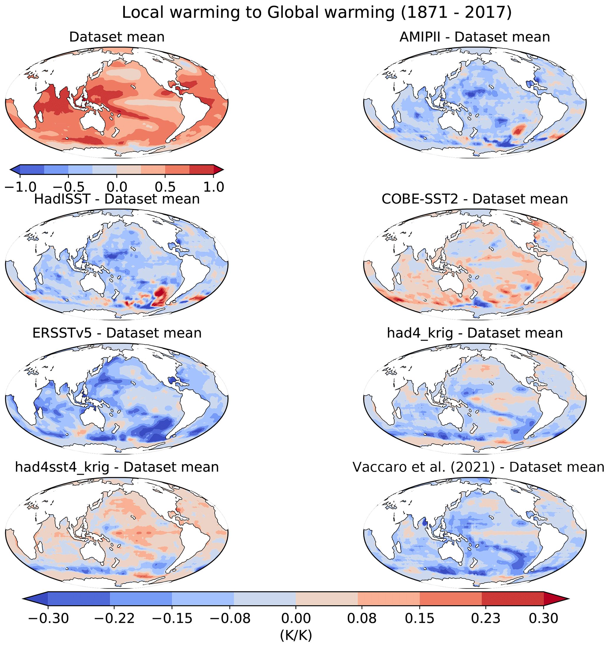
Figure 3 Change in the pattern of SST (change in T against the change in global mean T; in K K⁻¹) from 1871 to 2017 for each of the observedSST-piForcing simulations relative to the dataset mean.

We obtain ${\mathit{\lambda }}_{\mathrm{4}\times {\mathrm{CO}}_{\mathrm{2}}}$ and λ_hist from the corresponding AOGCM simulations piControl, abrupt4×CO₂ and historical which are available from the CMIP6 database for MPI-ESM1.2-LR. We perform a 150-year OLS regression of the global annual mean TOA net radiative flux change (N) against surface temperature change (T) to estimate ${\mathit{\lambda }}_{\mathrm{4}\times {\mathrm{CO}}_{\mathrm{2}}}$ as $-\mathrm{1.48}\pm \mathrm{0.03}$ W m⁻² K⁻¹ (Gregory et al., 2004). The changes are between the first 150 years of the abrupt4×CO₂ simulation and the mean of the last 500 years of the piControl simulation. Note that since we use surface temperature in our analysis, our estimate of ${\mathit{\lambda }}_{\mathrm{4}\times {\mathrm{CO}}_{\mathrm{2}}}$ for MPI-ESM1.2-LR is larger than the estimate from Zelinka et al. (2020) and Andrews et al. (2022), which used surface air temperature instead. For λ_hist, we take the changes between the global annual mean N and T of the entire period 1851–2014 of the historical simulation relative to the mean of first 50 years of the same. Since there are 10 ensemble members present in the historical simulation, we use the ensemble mean in our calculation. In addition, we conduct a simulation in fixed-SST configuration, but with evolving historical forcings to evaluate the effective radiative forcing (F) from 1851 to 2014. To calculate F, we account for the land surface warming: we subtract the product of ${\mathit{\lambda }}_{\mathrm{4}\times {\mathrm{CO}}_{\mathrm{2}}}$ and the land surface warming from N simulated by historical simulation in fixed-SST configuration (Hansen et al., 2005; Modak et al., 2018). We then regress N−F against T to estimate λ_hist as $-\mathrm{1.64}\pm \mathrm{0.07}$ W m⁻² K⁻¹ (Fig. 1).

4 Results and discussion

In the following we present the pattern effect estimated with the seven SST datasets, along with an inference of the unforced part. Then we discuss the differences between the datasets, and close by evaluating the impact of these new findings on estimates of ECS from historical warming.

4.1 Total pattern effect

The difference in feedback between the abrupt4×CO₂ and the observedSST-piForcing AGCM simulations is defined as the total pattern effect (Fig. 4a). We call it “total” to highlight the fact that the observedSST-piForcing AGCM simulations encapsulates the radiative effect of the spatial distribution of temperature, which depends on the all external forcings during the historical period as well as internal variability (Gregory et al., 2019; Seager et al., 2019; Watanabe et al., 2021; Lewis and Mauritsen, 2021). On the other hand, for a given model, the forced pattern effect can be derived from an ensemble of historical simulations. This pattern effect is the result of all forcing agents applied in the respective historical simulation. The difference between the “total” and “forced” could then be interpreted to be due to internal variability (discussed in next section). It is worth mentioning that while interpreting the temperature gradient in the equatorial Pacific, recent studies (e.g., Seager et al., 2019) have proposed that rising greenhouse gases are the cause for the observed temperature gradient. However, other studies support natural forcing and internal variability are equally possible causes (e.g., Gregory et al., 2019; Watanabe et al., 2021; Olonscheck et al., 2020).

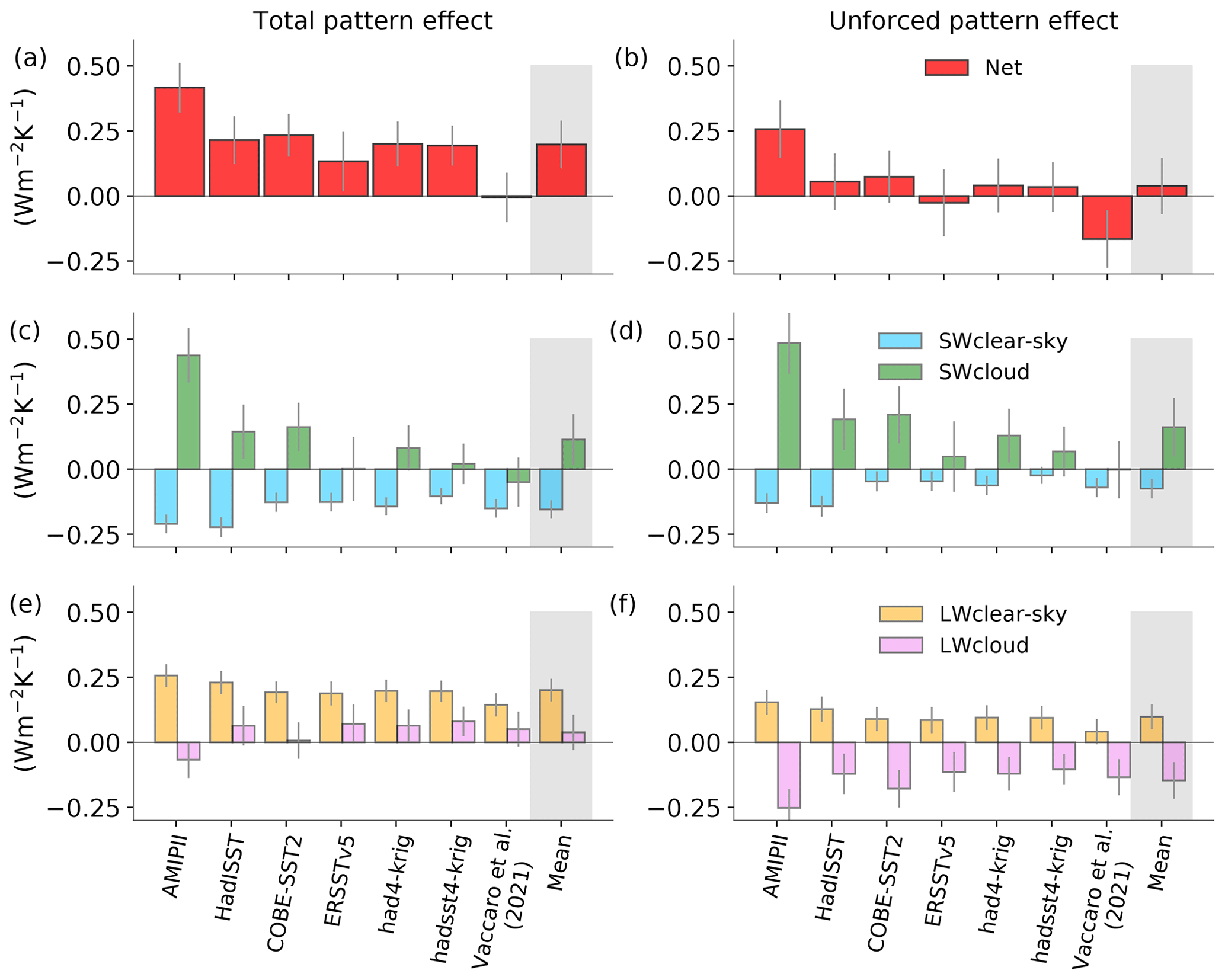
Figure 4 Estimates of total (a, c, e) and unforced pattern effect (b, d, f) and its shortwave (SW) and longwave (LW) radiative components from the seven observedSST-piForcing simulations from 1871 to 2017. Also shown is the dataset mean estimate in the gray shaded region. The error bars show ±1 standard error.

Depending on the underlying dataset, the strength of the total pattern effect ranges from $-\mathrm{0.01}\pm \mathrm{0.09}$ to 0.42±0.10 W m⁻² K⁻¹ over 1871–2017 while the mean estimate is 0.20 W m⁻² K⁻¹ [0.01 to 0.39 W m⁻² K⁻¹] (Fig. 4a). The uncertainty in the pattern effect estimates are calculated by adding the errors from ${\mathit{\lambda }}_{\mathrm{4}\times {\mathrm{CO}}_{\mathrm{2}}}$ and respective λ from observedSST-piForcing simulations in quadrature. A positive pattern effect would lead to a relatively less stabilizing feedback, i.e., a less negative λ and consequently a higher climate sensitivity. The mean estimate of the pattern effect derived from different dataset is less than the multi-model mean estimate of Andrews et al. (2022) and the mean estimate considered in the IPCC's Sixth Assessment Report (AR6; IPCC, 2021). Nevertheless, here one must keep in mind that MPI-ESM1.2-LR produces a slightly weaker pattern effect than that on average produced by other models. For example, Andrews et al. (2022) reported a value of 0.56 W m⁻² K⁻¹ for ECHAM6.3, the atmosphere component of MPI-ESM1.2-LR, whereas the multi-model mean was larger at 0.70 W m⁻² K⁻¹ with AMIPII (more discussion in Sect. 4.5). The differences in the pattern effect among the observedSST-piForcing simulations arises primarily due the differences in the shortwave (SW) cloud feedback (Fig. 4c). This is expected as the spatial pattern of temperature response primarily drives the circulation and the cloud response (Zhou et al., 2016; Ceppi et al., 2017; Mauritsen, 2016; Andrews and Webb, 2018). The large positive SW cloud pattern effect in the case of AMIPII compared to the rest of the datasets is responsible for inducing the overall larger net pattern effect.

We inferred the total pattern effect from Lewis and Mauritsen (2021) for the in-common SST datasets, which they calculated based on CAM5.3 Green's function (Fig. A2). We find that their estimates of total pattern effect are substantially different from our estimates for some of the SST datasets. The differences could be either because the Green's function that is applied in Lewis and Mauritsen (2021) is derived from a different model (CAM5.3 Green's function applied to ECHAM6.3) and different models produce different pattern effects or because of its inherent limitations (Zhou et al., 2017). However, we find that the uncertainty in the pattern effect estimates across the in-common SST datasets are of similar magnitudes between the studies. We plan to further address the comparison with the estimates derived from Green's function in a future study.

4.2 Unforced pattern effect

The unforced pattern effect, which represents the pattern effect due to the internal variability in the climate system, is defined as the difference in feedback between the historical and the observedSST-piForcing simulations, as discussed in the previous section. The rationale is that the observedSST-piForcing simulations could be one possible trajectory other than the fully coupled historical simulation.

Figure 5 Top panel shows the selected regions. Bottom panel shows the local warming compared to the warming over 50^∘ S–50^∘ N (K K⁻¹) from 1871 to 2017 for the observedSST-piForcing simulations. The selected regions are the Indo-Pacific Warm Pool (IPWP): 15^∘ S–15^∘ N, 45–195^∘ E; equatorial west Pacific (EWP): 15^∘ S–15^∘ N, 110–195^∘ E; equatorial east Pacific (EEP): 15^∘ S–15^∘ N, 195^∘ E–80^∘ W and Southern Ocean (SO): 35–60^∘ S. The error bars show ±1 standard error.

The dataset mean estimate of the unforced pattern effect is quite small, in agreement with Lewis and Mauritsen (2021), although it ranges from $-\mathrm{0.17}\pm \mathrm{0.11}$  to 0.26±0.11 W m⁻² K⁻¹: except for the AMIPII- and Vaccaro2021-based estimates, which lie at the two ends, all other datasets induce small values (Fig. 4b). In recent decades, we find strong dampening of the unforced pattern effect. The dataset mean estimate for the period 1970–2017 is 0.48±0.19 W m⁻² K⁻¹, for 1980–2017 it is 0.59±0.25 W m⁻² K⁻¹ and for the most recent period, 2000–2017, it is 0.29±0.48 W m⁻² K⁻¹. Thus, when inspecting short periods the unforced pattern effect can be substantial but across the century we find only small pattern effects.

4.3 Dataset differences

To investigate the differences in the strength of the pattern effect among the datasets, we compare the temperature trends over the Indo-Pacific Warm Pool (IPWP), equatorial west Pacific (EWP), equatorial east Pacific (EEP) and SO. The temperature trends over these key regions in the historical period typically stand in contrast to that in the long-term response (e.g., Andrews et al., 2018; Dong et al., 2019; Lewis and Mauritsen, 2021; Fueglistaler and Silvers, 2021). We find that the local warming compared to the warming over 50^∘ S–50^∘ N from 1871 to 2017 in each of these regions has significant differences in some cases among the datasets (Fig. 5). For instance, over the IPWP region, the ERSSTv5 dataset shows significant differences compared to HadISST, COBE-SST2, had4krig, hadsst4krig and Vaccaro2021. In the case of Vaccaro2021, the warming ratio is significantly different in all regions except over the EEP.

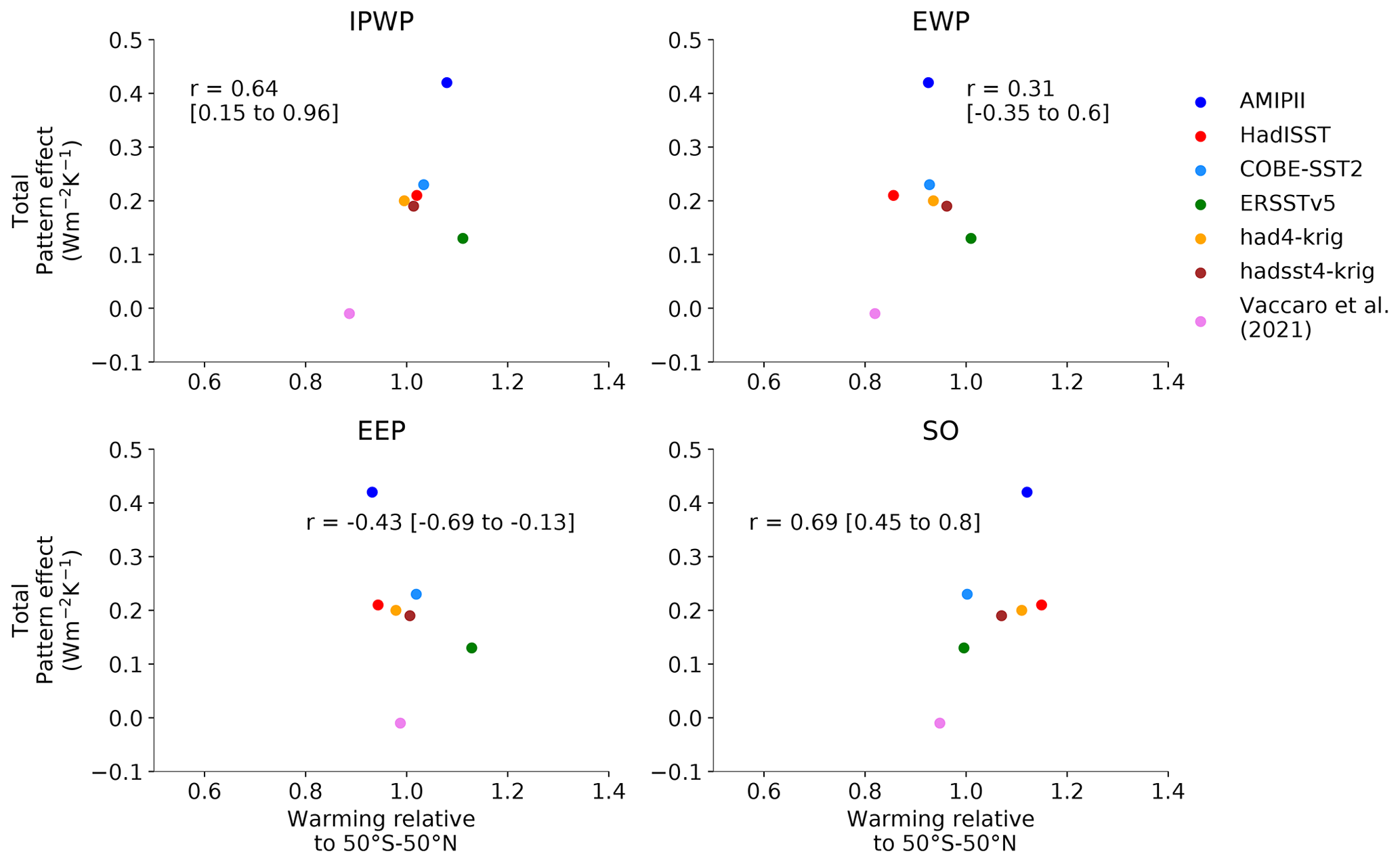
Figure 6 Relationship between the local warming in the selected regions to that over 50^∘ S–50^∘ N and the total pattern effect for the observedSST-piForcing simulations from 1871 to 2017. The selected regions are defined in Fig. 5. The Pearson correlation coefficient (r) is shown in the respective panels. The ranges show the correlation coefficient by removing one dataset at a time.

Past studies showed that the relative warming of the IPWP compared to the rest of the oceans or to the tropics could influence the strength of the pattern effect (Dong et al., 2019; Fueglistaler and Silvers, 2021; Lewis and Mauritsen, 2021). Dong et al. (2019) suggested that the IPWP governs the strength of the pattern effect as they found a strong dependence of the TOA radiation balance on the temperature over the IPWP. However, later it was found that such a clear dependence is not supported by the CMIP6 models (Dong et al., 2020; Lewis and Mauritsen, 2021). Across the datasets, we find a comparative correlation between the pattern effect and the regional warming relative to the 50^∘ S–50^∘ N: 0.64 over the IPWP, 0.31 over the EWP, −0.43 over the EEP and 0.69 over the SO (Fig. 6). Although AMIPII stands out from the rest of the datasets in its pattern effect strength, it does not show substantial differences in the relative warming except over the EEP and SO (Fig. 6c). However, both over the EEP and SO, even HadISST1, which simulates a relatively weak pattern effect, has relative warming similar to AMIPII. Thus, it is difficult to link the pattern effect variations across datasets only to IPWP warming; rather, we find all regions show a positive correlation, with the IPWP and SO showing a relatively stronger correlation than the EWP and EEP (Fig. 6).

To further investigate if any of the datasets bias the correlation, we calculate a range of correlation between the pattern effect and the relative warming by removing one dataset at a time. We find that over the IPWP the Pearson coefficient correlation (r) ranges from 0.15 to 0.96; in the absence of ERSSTv5, the correlation improves to 0.96, while without Vaccaro2021 it weakens to 0.15. Over the EWP, EEP and SO, the correlation ranges from −0.35 to 0.60, −0.69 to −0.13 and 0.45 to 0.80, respectively. Over the EWP without ERSSTv5, the correlation coefficient improves to 0.60; however, over the EEP without AMIPII, the correlation changes sign. Over the SO, the correlation coefficient is not sensitive to the datasets.

4.4 Temporal variation in pattern effect

Since the concept of the pattern effect comes from the time-evolving spatial structure of the surface temperature response, we regress N against T from the observedSST-piForcing simulations from 1871 to 1900 and then consecutively increase the regression length by 1 year to find the time-varying nature of the feedback (Fig. 7). Note that the final value of this feedback evolution is the 1871–2017 regression shown in Fig. 4a, c and e. We find that the feedback from the observedSST-piForcing simulations has a large spread in the early period until the 1940s, but in recent decades they agree more with each other. Unlike other datasets, feedback based on AMIPII starts to become more negative from the 1970s (Lewis and Mauritsen, 2021; Fueglistaler and Silvers, 2021). We find that feedback based on Vaccaro2021 also starts to drift relative to the rest from the 1970s (Fig. 7a), but in the opposite direction. It is apparent that the SW cloud feedback governs the evolution of the net feedback as shown in previous studies (Andrews et al., 2018; Fueglistaler and Silvers, 2021) and is primarily responsible for the behavior of feedbacks. Additionally, the spread in the early period is partly associated with the longwave (LW) cloud feedback (Fig. 7e).

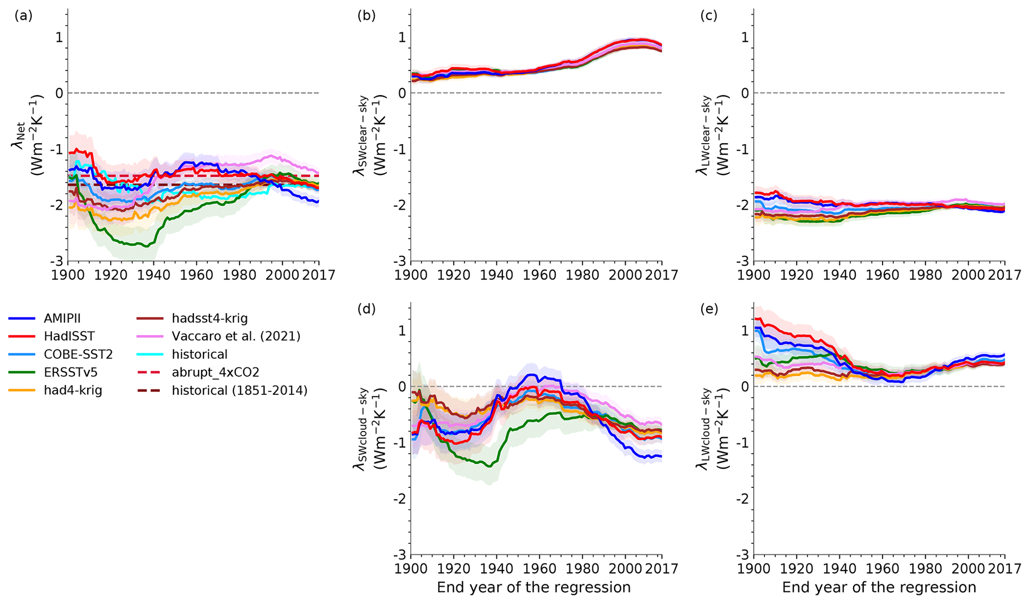
Figure 7 Net feedback (a), SW (b, d) and LW (c, e) components of feedbacks obtained by regressing the change in TOA radiative fluxes against the change in surface temperature from 1871 to 1900 and then consecutively incrementing the regression length by 1 year from the observedSST-piForcing simulations. The shading represents the ±1 standard error while the dashed lines in (a) shows ${\mathit{\lambda }}_{\mathrm{4}\times {\mathrm{CO}}_{\mathrm{2}}}$ and λ_hist. The cyan in (a) shows the time-varying λ_hist from the historical simulation, which denotes the forced pattern effect.

Another way to visualize the evolution of net feedback and its components is based on the regression of N against T in the sliding 30-year windows, shown in Fig. A3. We find that the feedback from all the observedSST-piForcing simulations is becoming less negative and consequently there is a smaller pattern effect in the most recent decade (Fig. A3a).

4.5 An updated estimate of ECS

We now illustrate how ECS constrained based on the instrumental record given in AR6 is updated when we account for dataset dependency (Fig. 8). We can integrate the pattern effect (Δλ) in the linear energy budget as $\mathrm{ECS}=-F_{\mathrm{2}x}/(\mathit{\lambda }+\mathrm{\Delta }\mathit{\lambda }$). In this section, note that we consider the best estimate while the uncertainty (standard deviation) and ranges denotes the 5 %–95 % confidence intervals. We apply the energy imbalance anomaly between 1850–1900 and 2006–2019 from AR6 as $\mathrm{\Delta }N=\mathrm{0.59}\pm \mathrm{0.35}$ W m⁻², the change in surface temperature as $\mathrm{\Delta }T=\mathrm{1.03}\pm \mathrm{0.20}$ K, the historical radiative forcing as ΔF=2.20 [1.53 to 2.91] W m⁻² and the ERF for doubling of CO₂ as $F_{\mathrm{2}\times }=\mathrm{3.93}\pm \mathrm{0.47}$ W m⁻². We account for the correlated uncertainties between the F_2× and the ERF for the well-mixed greenhouse gases. We infer the estimate of ERF of well-mixed greenhouse gases from AR6 as 1.73±0.29 W m⁻². The best estimate is obtained from the forcing data available from the IPCC AR6 GitHub repository. We deduced the uncertainty by taking the 5 %–95 % ranges of ERF of the well-mixed greenhouse gases from Fig. 7.6 of AR6 and adding them in quadrature.

Employing these values within the linear energy budget framework, we reproduce the constrained ECS estimate of 2.5 K [1.6 to 4.9 K] (Fig. 8). To compare the adjusted ECS derived based on our dataset-dependent pattern effect, we first apply the pattern effect used in AR6, 0.50 W m⁻² K⁻¹ [0.0 to 1.0 W m⁻² K⁻¹]. This updates the ECS to 3.6 K [1.9 to 13.7 K]. When we apply our dataset-dependent pattern effect estimate with the mean of the total pattern effect deduced from each dataset, 0.20 W m⁻² K⁻¹ [0.01 to 0.39 W m⁻² K⁻¹]), the ECS is adjusted to 2.9 K [1.7 to 6.7 K] (Fig. 8). As expected, this drops the best estimate and restricts the ECS range owing to the smaller pattern effect strength and uncertainty. However, the adjusted ECS with this pattern effect includes only the uncertainty due to different boundary conditions, which are based on the observed–reconstructed datasets and may be biased by the model. Andrews et al. (2022) estimated the pattern effect considering AMIPII and HadISST datasets. Here, we apply their pattern effect based on AMIPII only as they had amip-piForcing simulations from a greater number of models. They estimate the pattern effect to be (0.70 W m⁻² K⁻¹ [0.23 to 1.17 W m⁻² K⁻¹]), which when applied lifts the AR6 ECS to 4.3 K [2.1 to 19.3 K]. However, this only includes model uncertainty.

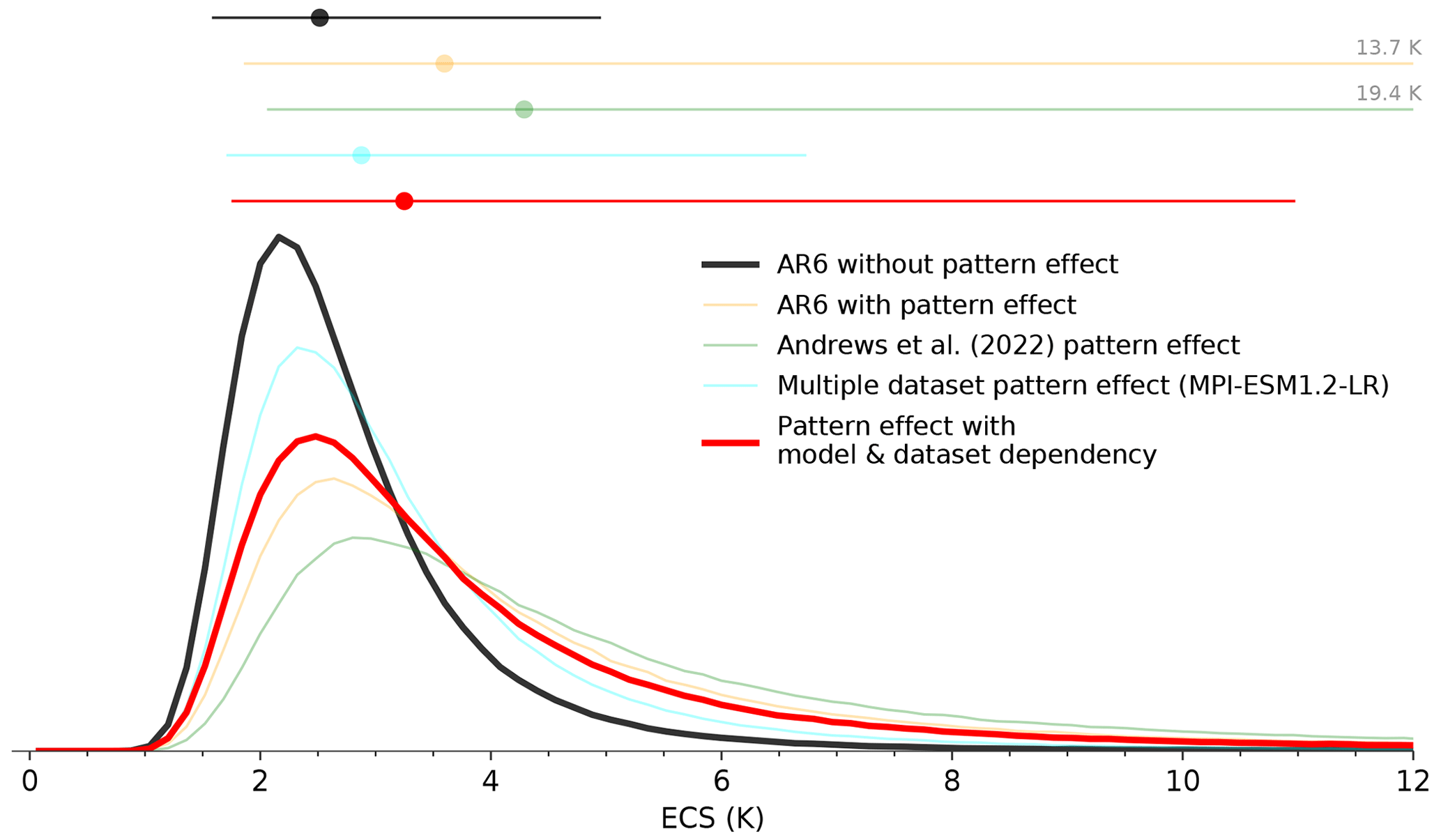
Figure 8 Probability distributions for ECS constrained based on the instrumental record of historical warming as per IPCC AR6 and updated with pattern effect estimates as indicated by the legend. AR6 without pattern effect estimate is the baseline for all the other estimates.

We therefore update the instrumental record-constrained ECS from AR6 with the combined pattern effect, which includes the pattern effect based on the dataset dependency as well as the intermodel spread from Andrews et al. (2022). We assume that the uncertainties from model and dataset dependencies are independent. We find the combined pattern effect estimate to be 0.37 W m⁻² K⁻¹ [−0.14 to 0.88 W m⁻² K⁻¹]. The combined estimate is obtained by subtracting the mean of ECHAM6.3 and MPI-ESM1.2-LR estimate in Andrews et al. (2022) from the sum of our estimate and their multi-model mean estimate. The uncertainty range in the combined estimate is deduced by adding in quadrature the standard deviations from our dataset-dependent estimate and their multi-model estimate. Thus, our calculation also accounts for the weaker pattern effect in ECHAM6.3 and MPI-ESM1.2-LR compared to the multi-model mean. While accounting for the weaker pattern effect, the assumption is that ECHAM6.3/MPI-ESM1.2LR is different from all the other models in all datasets as in AMIPII. However, one can dispute this assumption. We infer from Andrews et al. (2022) and examine this. We show in Fig. A4 that not only ECHAM6.3/MPI-ESM1.2LR but also other models, though producing a stronger pattern effect, show a similar difference in pattern effect estimates based on AMIPII and HadISST datasets as in ECHAM6.3/MPI-ESM1.2LR. Nevertheless, when we apply the combined pattern effect, we find that the constrained ECS based on historical warming is adjusted to 3.2 K [1.8 to 11.0 K] (Fig. 8), which is slightly smaller and better constrained than in the instrumental record estimate of IPCC AR6.

5 Conclusions

Observed historical warming provides an opportunity to estimate Earth's ECS. However, our ability to constrain ECS based on it is limited both by the uncertainty in aerosol cooling and by the strength of the pattern effects. Pattern effects temporarily dampen transient global warming and so factoring this leads to larger and less-constrained ECS estimates. Recent studies have estimated the model dependence of the pattern effect strength using a range of models with prescribed SSTs primarily from the AMIPII observed–reconstructed dataset. Here we instead investigated the dataset dependence using a single model with seven different datasets. The resulting spread is substantial, although smaller than that among different models, and it turns out that the pattern effect estimated from the AMIPII dataset is by far the largest, suggesting that earlier studies may have overestimated the pattern effect. However, we reiterate that any of the SST dataset could be a possible path Earth could have taken.

The datasets differ due to the measurement sources, methods applied to merge datasets and infilling techniques. Depending on the applied datasets, we find that the total pattern effect varies from $-\mathrm{0.01}\pm \mathrm{0.09}$ to 0.42±0.10 W m⁻² K⁻¹ over 1871–2017, while the mean across the datasets is 0.20 W m⁻² K⁻¹ [0.01 to 0.39 W m⁻² K⁻¹]. The mean unforced pattern effect across the dataset is generally small although it ranges from $-\mathrm{0.17}\pm \mathrm{0.11}$ to 0.26±0.11 W m⁻² K⁻¹. As expected, differences in the pattern-effect is primarily attributed to differences in the cloud radiative effects. While the estimates from the 1970s until present are less dataset dependent, the major disparities originate in the early period and are driven by cloud feedback. By assuming the variations in model and dataset dependencies are independent, we then estimate a combined pattern effect of 0.37 W m⁻² K⁻¹ [−0.14 to 0.88 W m⁻² K⁻¹]. Taking global warming, radiative forcing and imbalance from AR6, this results in a historical warming-constrained ECS estimate of 3.2 K [1.8 to 11.0 K], which is better constrained than that of AR6 as a result of the slightly weaker mean pattern effect.

In the community currently, the prevailing understanding is that the strength of the pattern effect is related to the temperature response over the IPWP. However, here we find a comparative correlation between the pattern effect strength and the relative warming trends over all of the IPWP, EWP, EEP and SO and those over 50^∘ S–50^∘ N across the datasets. Thus, we are unable to identify specific regions that could govern the strength of the pattern effects and it is difficult to co-locate patterns of surface temperature change and the strength of the pattern effect between the datasets.

In the current study we had to assume that the variations in the pattern effect as estimated among the models and across the datasets are independent of each other in order to provide a combined estimate of the pattern effect. However, one could raise the concern that a single model will not completely display dataset dependency. In particular, the model we used here is correlated less well with the observed SW anomalies in Loeb et al. (2020). Therefore, we have decided in extension to conduct a multi-model and multi-dataset intercomparison project to address this outstanding concern.

Appendix A

(Rayner et al., 2003)(Hurrell et al., 2008)(Hirahara et al., 2014)(Huang et al., 2017)(Cowtan and Way, 2014)(Morice et al., 2012)(Cowtan and Way, 2014)(Vaccaro et al., 2021a)(Morice et al., 2012)(Vaccaro et al., 2021a)

Table A1 List of observed SST datasets applied to MPI-ESM1.2-LR in this study.

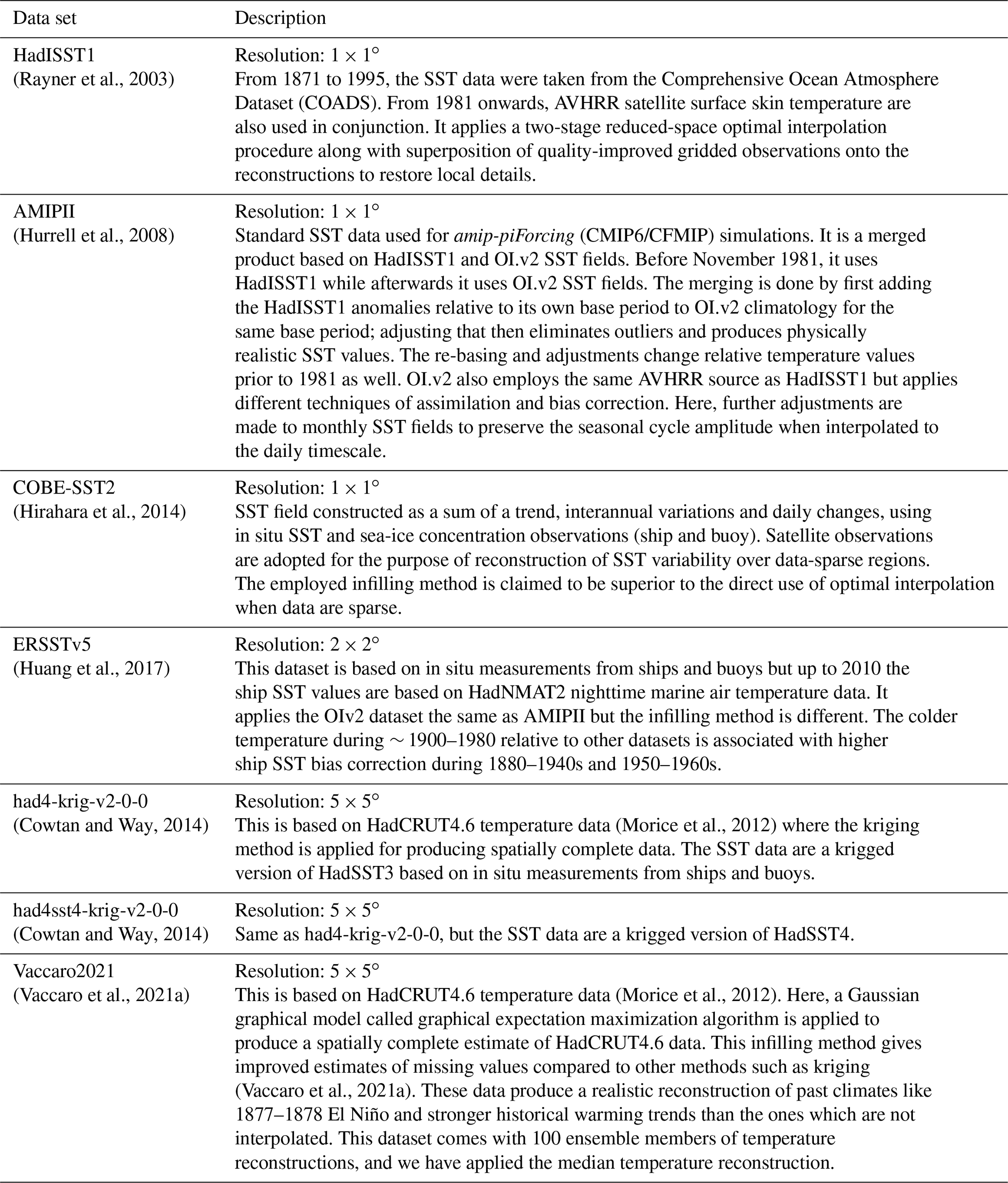
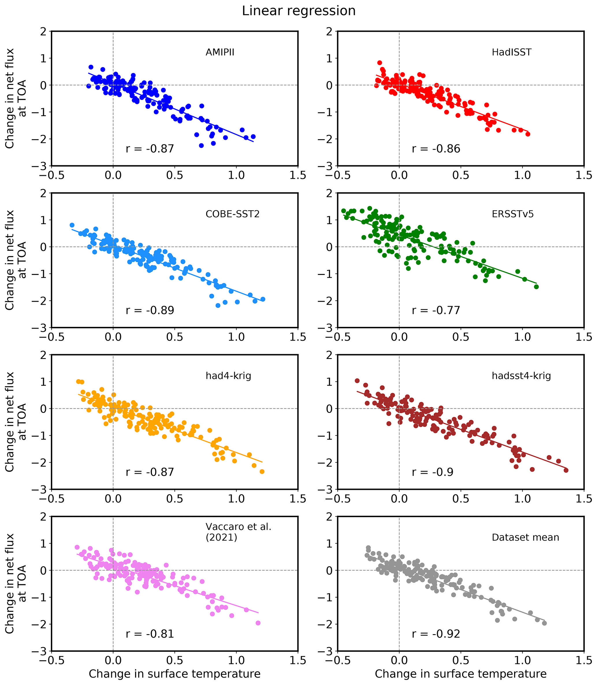
Figure A1 Linear regression between the change in global annual mean net downward radiation flux at TOA against surface temperature change (Gregory et al., 2004) for the observedSST-piForcing simulations. The changes are relative to the 1871–1900 mean. The Pearson correlation coefficient (r) is shown for each panel.

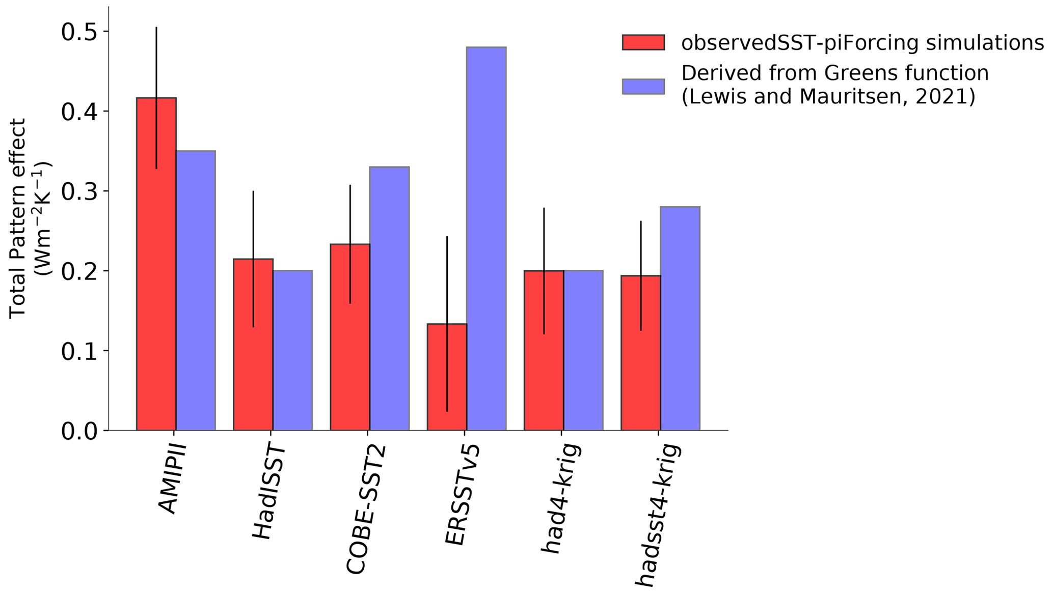
Figure A2 Comparison of total pattern effect estimated from the observedSST-piForcing simulations (as in Fig. 4a) and inferred from Lewis and Mauritsen (2021) for the in-common SST datasets.

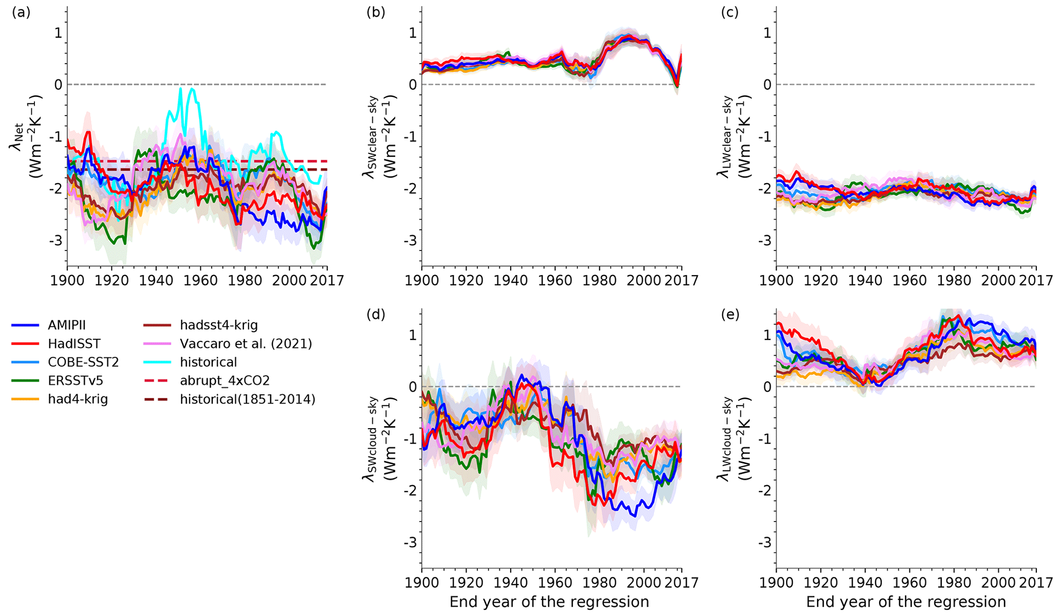
Figure A3 Net feedback obtained by regressing the change in TOA radiative fluxes against the change in surface temperature with a sliding 30-year period from 1871 to 2017 from the observedSST-piForcing simulations. The shading represents the ±1 standard error while the dashed lines in (a) show ${\mathit{\lambda }}_{\mathrm{4}\times {\mathrm{CO}}_{\mathrm{2}}}$ and λ_hist. The cyan in panel (a) shows net feedback from historical simulation for MPI-ESM1.2-LR.

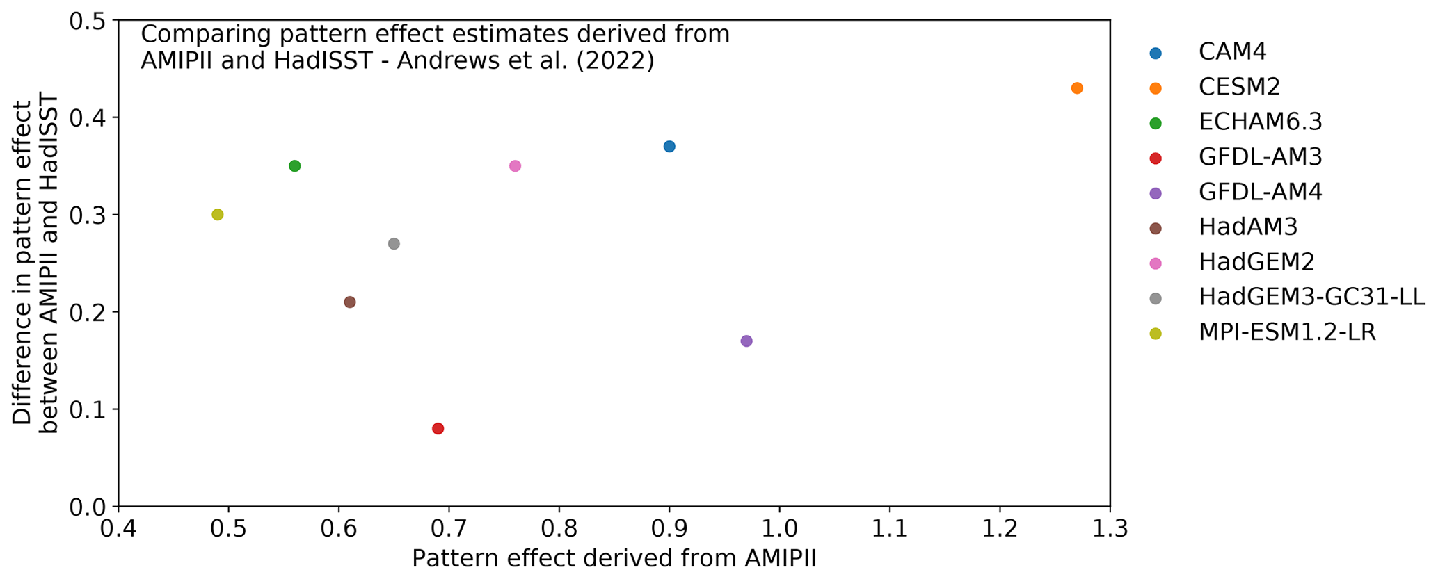
Figure A4 Difference in the total pattern effect estimates derived from AMIPII and HadISST datasets for a given model against its total pattern effect estimate based on AMIPII. Shown for all models (in legend) from Andrews et al. (2022).