Simulated long-term evolution of the thermosphere during the Holocene – Part 2: Circulation and solar tides

On timescales longer than the solar cycle, long-term changes in CO₂ concentration and geomagnetic field have the potential to affect thermospheric dynamics. In this paper, we investigate the thermospheric dynamical response to these two factors during the Holocene, using two sets of ∼12 000-year control runs by the coupled thermosphere–ionosphere model, GCITEM-IGGCAS. The main results indicate that increased/decreased CO₂ will enhance/weaken the thermospheric circulation throughout the Holocene, but this effect is non-linear. The cooling effect of CO₂ in the thermosphere further provides plausible conditions for atmospheric tidal propagation and increases the thermospheric tidal amplitude. Geomagnetic variations induce hemispheric asymmetrical responses in the thermospheric circulation. Large changes in the circulation occur at high latitudes in the hemisphere with distant magnetic pole drift, inferring a crucial role of geomagnetic non-dipole variations in circulation changes. A positive correlation between the diurnal migrating tide (DW1) and geomagnetic dipole moment is revealed for the first time. The amplitude of DW1 in temperature will increase by ∼1–3 K for each 1×10²² A m² increase in dipole moment.

1 Introduction

The main external energy input to the terrestrial thermosphere is solar radiation, particularly in the extreme ultraviolet (EUV) band. The solar-driven circulation manifests as the flow across the isobars, in contrast to the geostrophic flow that dominates in the middle and lower atmosphere (Forbes, 2007). This is because the Coriolis force is much smaller than the pressure gradient term for the typical terrestrial thermosphere. Under absorption of solar daily cyclic forcing, the atmosphere also induces the solar tides, which refers to global-scale perturbations in atmospheric parameters with periods and zonal wavenumbers that are harmonics of a day and a zonal cycle. In addition to the local absorption of EUV radiation as the major source, the solar tides in the thermosphere also come from upward propagating waves excited in the middle and lower atmosphere, including the infrared absorption by tropospheric H₂O and ultraviolet absorption by stratospheric O₃ (Forbes and Zhang, 2022). Thus, the level of solar activity is expected to have a key impact on the dynamical variability in the thermosphere (Oberheide et al., 2009; Sun et al., 2022). However, when inspecting on timescales longer than the solar cycle, the influence from other secular variables, such as long-term changes in CO₂ concentration and main geomagnetic fields, should not be ignored. It is then natural to ask how and to what extent these factors act on the thermospheric dynamics on long-term timescales, e.g., since the beginning of the Holocene.

CO₂ plays a significant role in cooling the thermosphere, in contrast to the warming effect in the troposphere (Laštovička et al., 2006; Solomon et al., 2018). Since the first prediction by Roble and Dickinson (1989), many observational evidences and simulation experiments have been subsequently proposed to support the CO₂ cooling effect using modern techniques and advanced models (Akmaev and Fomichev, 2000; Akmaev et al., 2006; Marsh et al., 2013; Ogawa et al., 2014; Qian et al., 2006, 2011; Solomon et al., 2015; Zhang et al. 2016). A well-established consensus is that every 10 ppm increase in CO₂ concentration will result in a ∼1–3 K decrease in global mean temperature in the thermosphere (e.g., Solomon et al., 2018). As the issue of increasing CO₂ becomes urgent (IPCC, 2014), researchers have also worked to elucidate the concomitant effects on the upper atmosphere (Zhou et al., 2022), and one of which is the thermospheric dynamics. Using the GAIA (Ground-to-topside Atmosphere Ionosphere model for Aeronomy) simulation, Liu et al. (2020) suggested that the doubling of CO₂ concentration should strengthen thermospheric meridional circulation, enhance diurnal migrating tide, and weaken semidiurnal migrating tide. Kogure et al. (2022) further analyzed the underlying mechanism of the thermospheric zonal mean wind response, suggesting that the ion drag, molecular viscosity, and meridional pressure gradient forces as the three main factors are in the combined modulation. However, the impact of CO₂ on the long-term evolution of the thermospheric dynamics during the Holocene is still poorly understood.

The secular variation of the geomagnetic field would produce considerable changes in the thermosphere temperature other than the CO₂ effect. Although the geomagnetic variation does not act directly on the neutral atmosphere, it affects ion motion and thus ionospheric behavior (Cai et al., 2019; Elias et al., 2022; Yue et al., 2018; Zossi et al., 2018), which are coupled to the neutral atmosphere via ion-neutral collisions. The strength of the geomagnetic field determines the gyrofrequency and the ionospheric conductivity, thus influencing the Joule heating power and E×B drift velocities (Cnossen et al., 2012; Zhou et al., 2021). The geomagnetic tilt angle controlling the geographic distribution of the Joule heating should produce further changes in temperature and neutral winds (Cnossen and Richmond, 2012). The secular changes of geomagnetic field produce regionally both positive and negative changes; therefore in the global average their effect is negligible (Qian et al., 2021). Cnossen (2014) reported that the geomagnetic variation over the last century could cause a $\sim \pm \mathrm{10}$ K change in the thermosphere temperature regionally, comparable to the −8 K decrease in global temperature due to increased CO₂ over the same period. Analyses of recent decades (Cnossen et al., 2020) and projections in the coming decades (Cnossen, 2022) about the thermospheric climate change confirm the importance of the geomagnetic variation, although accelerating CO₂ growth still plays a dominant role. Since the geomagnetic field has undergone a more complex evolution during the Holocene than in the present century (Korte et al., 2011), the impact on the evolution of thermospheric dynamics is expected to be more dramatic and therefore worth investigating.

The aim of the present study is to discuss the scenario of thermospheric dynamic changes due to the long-term changes in CO₂ concentration and geomagnetic field during the Holocene. This paper is organized as follows: Sect. 2 will briefly introduce the numerical simulation settings. Section 3 will show the main results of the simulations, then Sect. 4 discusses the scientific key points. In the end, a short summary is given in Sect. 5.

2 Model description and settings

Attempting to understand the long-term evolution of thermospheric dynamics affected by these two factors in the Holocene, we designed long-term time-slice simulations based on the Global Coupled Ionosphere–Thermosphere-Electrodynamics Model developed at the Institute of Geology and Geophysics, Chinese Academy of Sciences (GCITEM-IGGCAS; Ren et al., 2009, 2010, 2011, 2020). Detailed model description and settings are referred to in Yue et al. (2022) and Cai et al. (2023), which have carefully investigated the global thermal structure and density profile of the thermosphere and ionosphere, respectively. Here, we give a brief introduction to restate and to add key information. This 3-dimensional coupled thermosphere–ionosphere model self-consistently solves the global thermospheric and ionospheric behavior in the altitudinal coordinate, covering altitudes from 90 to 600 km. The ionospheric electro-dynamics are solved on the provided geomagnetic field configuration using magnetic apex coordinates (Richmond, 1995) based on a set of spherical harmonic coefficients. The calculation scheme requires the geomagnetic field to be dipole-dominated, so the situation of geomagnetic reversal is difficult to portray. The high-latitude electric potential and electric fields are specified by the empirical model of Weimer-96 (Weimer, 1996), which is driven by the hemispheric power (HP), solar wind speed (SWS), interplanetary magnetic field (IMF), and cross-polar cap potential (CPCP). At the lower boundary at 90 km, migrating tides in neutral temperature and density are given by the global-scale wave model (GSWM), while neutral winds are self-consistently calculated. Non-migrating tides are not included in this study. The solar EUV radiation is described by the empirical model EUVAC (Richards et al., 1994), which is driven by the proxy of solar flux at 10.7 cm (F_10.7). The CO₂ cooling is calculated under the assumption of the non-local thermodynamic equilibrium (NLTE) with a cooling-to-space approximation assumed. In this model, the CO₂ level is specified by a given value for a fixed time under the assumption of diffusive equilibrium. This calculation formula follows Roble et al. (1988) and is also adopted by other thermosphere–ionosphere coupled models, such as NCAR-TIEGCM (Qian et al., 2017).

To diagnose the long-term effects of CO₂ and geomagnetic field variations on the thermospheric dynamics, two control runs (CR1 and CR2) were performed under perpetual solar minimum and geomagnetic quiet conditions, which correspond to the CR2 and CR1 in Yue et al. (2022) and Cai et al. (2023). The driving parameters in the Weimer-96 model are set as HP = 10 GW, SWS = 300 m s⁻¹, IMF By = 0 nT, IMF Bz = −0.5 nT, and CPCP = 20 kV for both cases, representing the extreme geomagnetically quiet condition of $Kp=\sim \mathrm{0.3}$. To eliminate the impact of solar variation, each case was performed under solar minimum, corresponding to the F_10.7 setting to be a constant of 87 sfu (solar flux unit; 1 sfu = 10⁻²² W m⁻² Hz⁻¹). In CR1, realistic CO₂ from a combined dataset drives the GCITEM-IGGCAS model with a fixed configuration of geomagnetic fields. Hence, the simulated variability of the thermosphere is derived exclusively from the CO₂ changes. The CO₂ dataset consists of three components: (1) estimations from the ice cores' recorded air composition since ∼80 000 years before the present with a rough resolution of ∼100 years during the Holocene (Lüthi et al., 2008); (2) measurements in ice with high precision back to 2000 years before the present (MacFarling Meure et al., 2006); and (3) modern atmospheric measurements at Mauna Loa Observatory, Hawaii, since 1958 (Keeling et al., 1995). In CR2, the CO₂ level is fixed to be 270 ppm, corresponding to the averaged value during the Holocene, while the geomagnetic fields are set to be varied with time. The specified geomagnetic field before 1900 is provided by the CALS10k.2 model developed by Constable et al. (2016), which is based on the archeo-magnetic and lake sediment data. Generally, this model roughly has spherical harmonics to degree and order of 10, and cubic B-splines parameterization is implemented with knots positioned every 40 years. After 1900, the geomagnetic fields are described by the International Geomagnetic Reference Field (IGRF) model (Alken et al., 2021). This model is based on the modern magnetic observations to describe the spatial distribution of geomagnetic fields by the spherical harmonic degree and order of 13 with the time resolution of 5 yrs. The secular variation of the geomagnetic field implemented in the CR2, including the dipole moment and the position of magnetic and geomagnetic poles, was illustrated in Fig. 1 of Yue et al. (2022), and the readers could refer to Constable et al. (2016) for more detailed information. A general scenario includes: (a) that the dipole moment fluctuated within 6.1–10.1 (10²² A m²) and has continuously decreased since 1700 by ∼13 %, and (b) that the geomagnetic/magnetic pole is located at latitudes larger than $\mathrm{78}/\mathrm{70}$^∘ and has drifted from the Western Hemisphere to the Eastern Hemisphere over the past century. Both cases were run every 100 years in the period of 9455 BC to AD 1945, and an additional run of AD 2015 was for the contemporary condition. Particularly, pre-runs of 15 d were performed as spin-up preparation to eliminate the influence from the initial conditions, and the outputs in the last day were used for analysis. Each case was running in two seasons, March and June, with the aim of discussing the seasonal dependence of the thermospheric dynamical response.

3 Results

3.1 CO₂ effect

According to the CR1 results, Fig. 1 illustrates the changes in zonal mean winds due to increased CO₂ from 1945 to 2015 (310 to 400 ppm), exemplifying how the changes in CO₂ act on the thermospheric circulation. Figure 1b–d shows the strengthening of the thermospheric circulation in March, mainly including enhanced equatorward flow from the North and South poles, accelerated eastward flow at middle and low latitudes, and increased downward/upward movement in the upper/lower thermosphere. The acceleration of the eastward zonal and equatorial meridional winds is about ∼1–2 m s⁻¹ when CO₂ is increased by ∼90 ppm. The CO₂ acceleration effect of the thermospheric circulation is also evident in June. Figure 1f–h shows the enhanced summer-to-winter prevailing wind and corresponding increased westward/eastward zonal wind in the summer/winter hemisphere due to the Coriolis force. The vertical winds also show a downward increase in the upper thermosphere, while the slight increase in the lower thermosphere disappears around the winter pole. Compared to the wind change in March, the accelerated thermospheric winds in June achieve ∼2–3 m s⁻¹ in zonal and meridional and a few cm s⁻¹ in vertical winds. Our simulation gives a reasonable and convincing result compared to the GAIA simulation of Liu et al. (2020), which shows an increase in the meridional winds of 5–15 m s⁻¹ when CO₂ increases by 345 ppm.

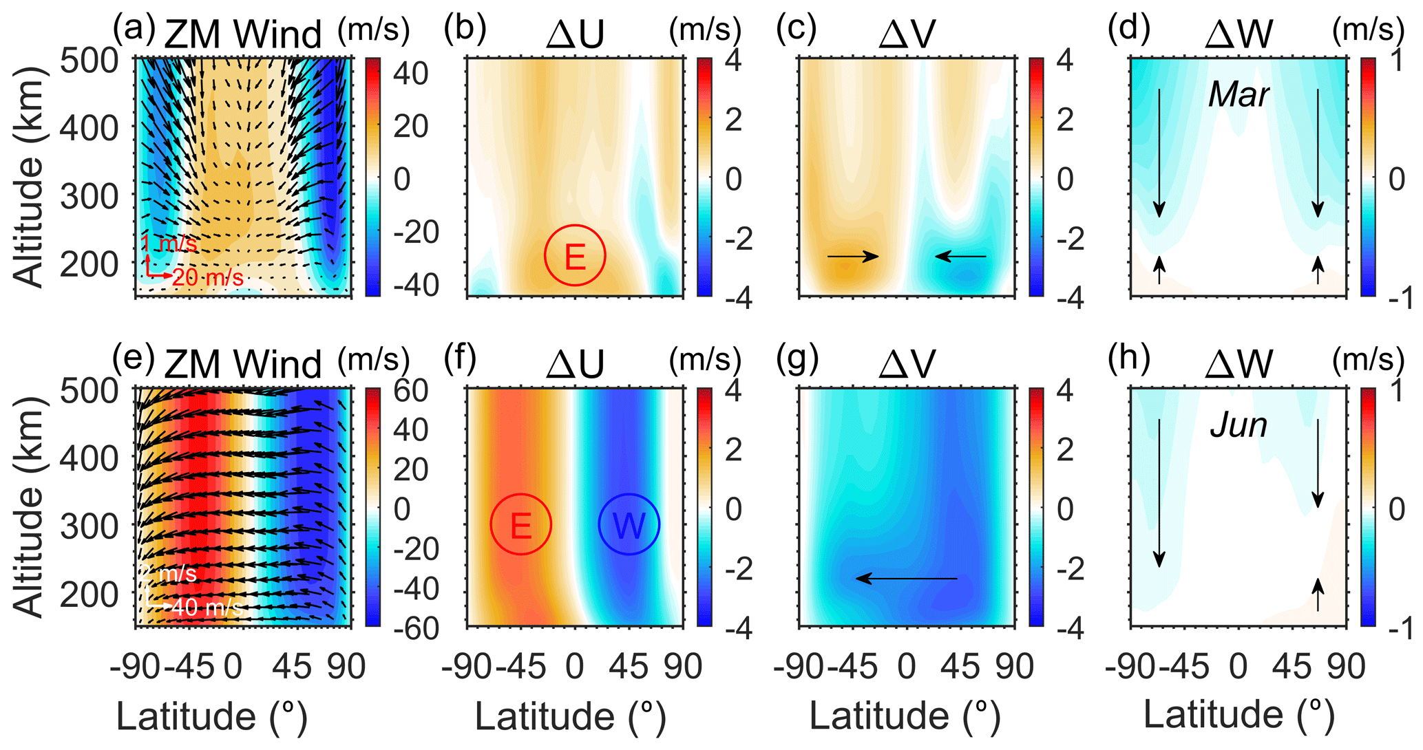
Figure 1 (a) Thermospheric circulation is illustrated by colors (zonal) and arrows (meridional and vertical) in March 2015. (b–d) Changes in zonal, meridional and vertical wind velocity due to the increase of CO₂ from 1945 to 2015. Plots (e) and (f) are the same as plots (a)–(d) but for June.

Examining the CO₂ effect on the thermospheric circulation throughout the Holocene, Fig. 2 illustrates the time evolution of changes in meridional wind versus latitudes in the CR2 simulation. The chosen height of ∼197 km is where the changes in the meridional wind are significant as shown in Fig. 1. The results for the beginning year (−9455) have been subtracted in order to show the CO₂ effect more intuitively. The corresponding CO₂ variation is plotted as the solid red line, which also subtracts the CO₂ level in the beginning year (264 ppm). Changes in the meridional circulation are obviously highly correlated with CO₂ variation and become much more significant since ∼ 1800 when the increase in CO₂ was much larger due to the industrial revolution. The correlation coefficient is generally over ±0.99 at most latitudes. During the equinox season, the meridional circulation tends to be more/less equatorward due to the increase/decrease of CO₂. As for the solstice season, the CO₂ effect manifests as acceleration/deceleration of the summer-to-pole circulation. For the past over 10 000 years before ∼ 1800, the change in meridional circulation velocity in March and June only fluctuated by ∓0.4–±0.1 m s⁻¹ and −0.6 to −0.2 m s⁻¹, respectively. However, in the last 200 years, the CO₂-induced changes in meridional wind could reach more than 1 m s⁻¹. Figure 3 further analyses the CO₂ effect on the thermospheric dynamics, choosing the averaged zonal circulation as a proxy. The results show that CO₂ enhances the eastward flow at the Equator during March, rather than being strictly linear. The growth of the accelerated eastward flow becomes small as CO₂ increases. Linear regressions show a change of 0.012 m s⁻¹ in the thermospheric equatorial zonal flow per parts per million CO₂ increase, and the parabolic fit should be in good agreement with the simulated data. The parabolic fitting obviously indicates that the rate of change of the thermospheric circulation slows down at the present CO₂ level. A similar non-linear effect is also manifested in the June zonal circulation (Fig. 3c).

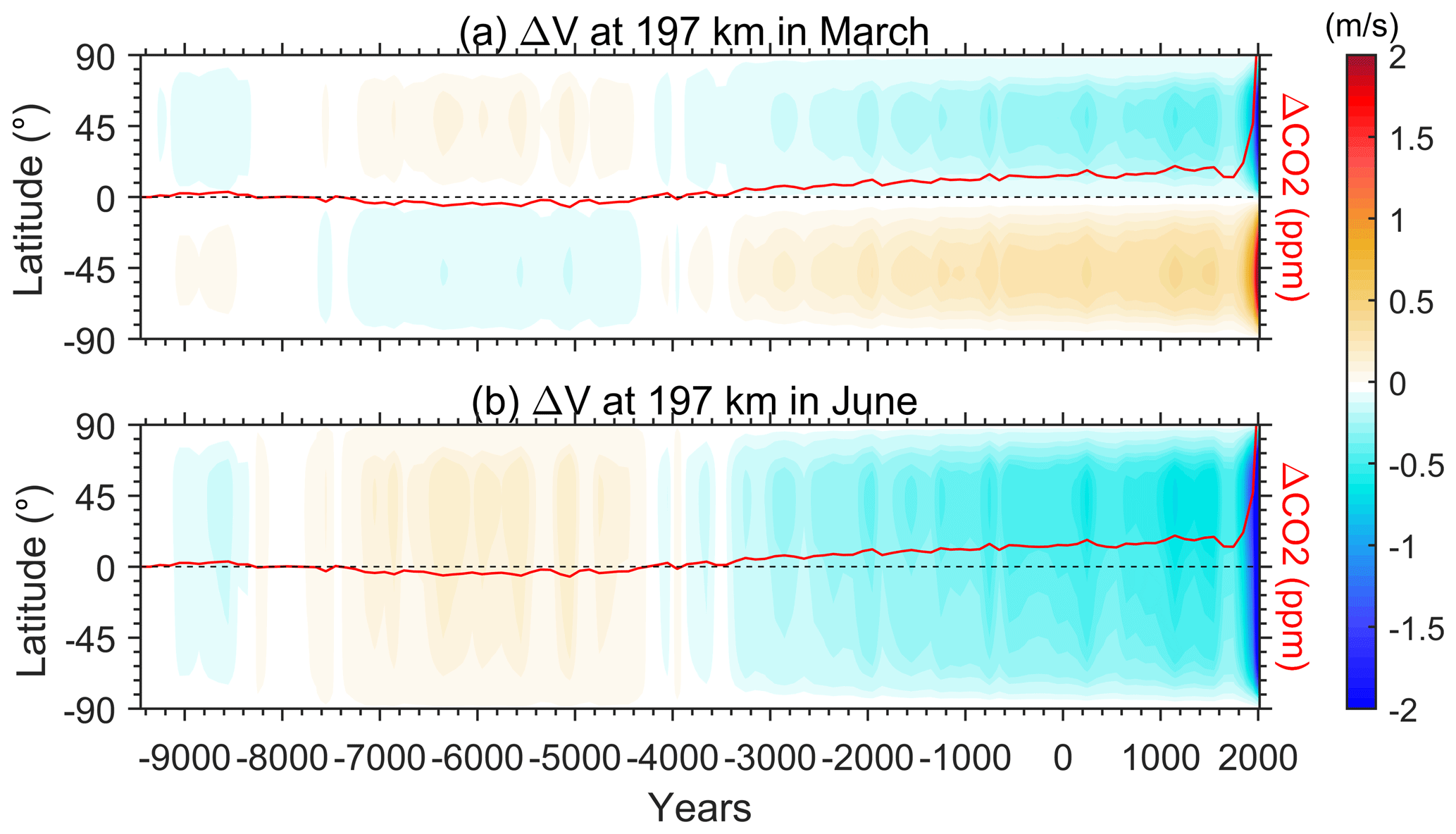
Figure 2 Time evolution of the changes in the zonal mean meridional wind at 197 km during (a) March and (b) June. The corresponding CO₂ variation is plotted in the solid red line.

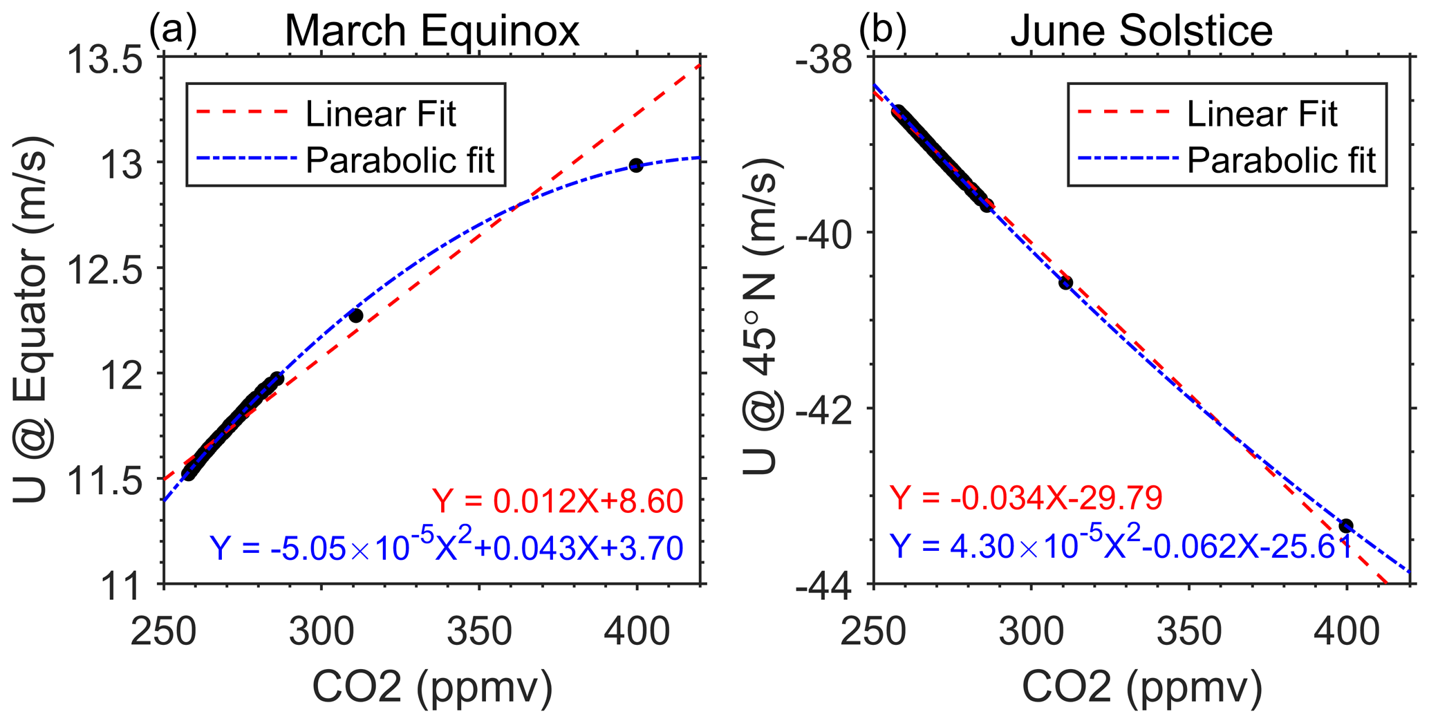
Figure 3 Response of thermospheric zonal mean zonal winds (150–600 km average) to the CO₂ increase (a) at the Equator in the March equinox and (b) at 45^∘ N in the June solstice. Linear and parabolic fitting are indicated in dashed red lines and dash-dotted blue lines, respectively.

As for the solar tidal response to the CO₂ variation during the Holocene, Fig. 4 illustrates the time evolution of diurnal migrating tide in temperature (DW1−T) at ∼240 km, which is the major tidal component in the thermosphere. The DW1−T tidal amplitude is positively correlated with CO₂ changes, manifesting as increasing by ∼10 K compared with the beginning year (−9455) during March when the CO₂ levels achieve 400 ppm in the modern era, particularly maximizing at the equatorial and low-latitude region. From 8000 BC to 4000 BC, when the CO₂ level was low throughout the Holocene, the DW1−T amplitude also decreased slightly. The specified DW1−T amplitude at the lower boundary in March is a maximum of ∼16 K at the Equator and two secondary peaks of ∼7 K at ±35^∘. As for the DW1−T at the lower boundary in June, the strength is $\sim \mathrm{1}/\mathrm{2}$ of that during March. Correspondingly, the changes in the thermospheric DW1−T amplitude in the modern era are slightly over 2 K, only $\sim \mathrm{1}/\mathrm{4}$ of that in March. The maximum change is found at middle latitudes in the winter hemisphere, rather than the Equator. The latitudinal difference in the DW1−T changes is contrary to the DW1−T time tendency, which generally maximizes in the summer hemisphere (Gu and Du, 2018).

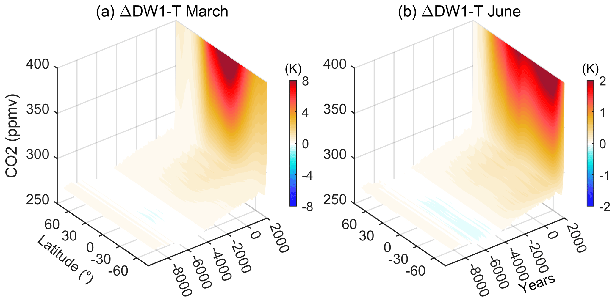
Figure 4 Change in the amplitude of diurnal migrating tide (DW1) at 240 km due to the CO₂ variation in (a) March and (b) June with respect to the beginning of the simulation.

'

3.2 Geomagnetic field effect

The geomagnetic field effect on the thermospheric circulation is regional and complicated, unlike the global effect of CO₂. Figure 5 exemplified the thermospheric circulation in the present era in the CR2 simulation and manifested how the circulation changed over the past 70 years due to the geomagnetic variation. The thermospheric winds generally flow across the isotherm due to the pressure gradient force and can maximize over 100 m s⁻¹ around the terminator. The auroral heating modulates the solar-driven winds and decreases the poleward flow at high and middle latitudes. Figure 5b shows that the geomagnetic variation from 1945 to 2015 alters the geographic distribution of temperature in March, notably at high latitudes ($\sim \pm \mathrm{15}$ K) and not negligibly at middle and low latitudes (±5 K). Correspondingly, the change in horizontal neutral winds could exceed 30 m s⁻¹ at high latitudes and around the dusk sector. The changes in temperature and wind induced by the geomagnetic field are smaller in June than that in March, which is about $\pm \mathrm{10}/\pm \mathrm{3}$ K at high/middle–low latitudes for temperature and maximizes ∼20 m s⁻¹ for horizontal winds. The circulation change shows a larger change in the Northern Hemisphere than in the Southern Hemisphere, in both simulations for March and June. The horizontal wind changes in the Southern Hemisphere are generally smaller by 10–20 m s⁻¹ than that in the Northern Hemisphere, and the temperature change is smaller by 5–10 K. The hemisphere difference is coincident with the asymmetrical change in the geomagnetic poles. The northern magnetic pole shifted 12 and 76^∘ in latitude and longitude, respectively. However, the southern magnetic pole drifted by merely 4 and 7^∘ in latitude and longitude, respectively.

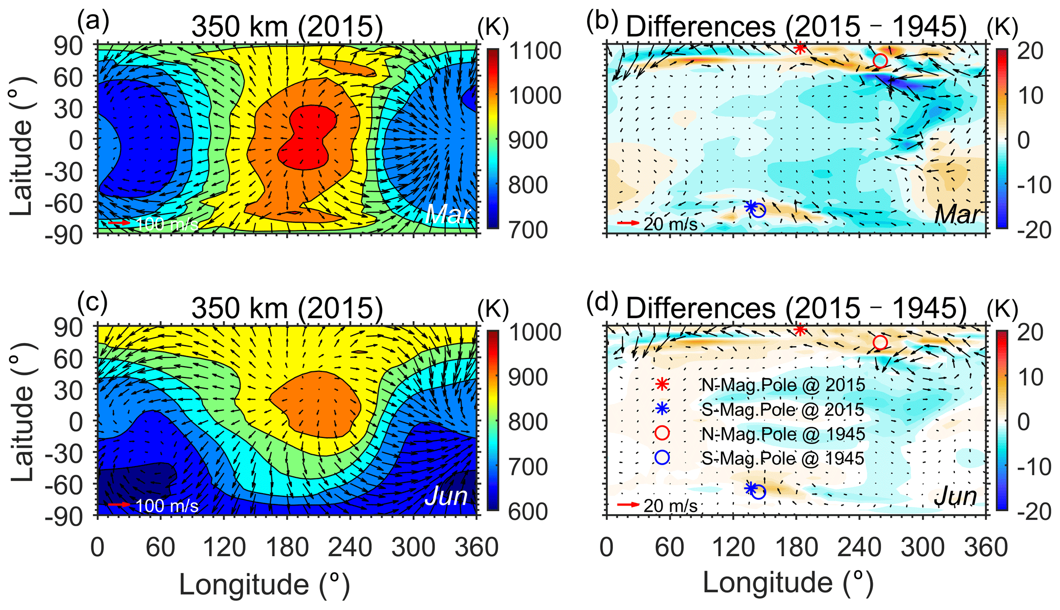
Figure 5 Geographic distribution of neutral temperature (color contours) and horizontal winds (black arrows) at 350 km in (a) March and (c) June at 00:00 UT. (b) Differences in neutral temperature and horizontal winds due to changes in geomagnetic field between 1945 and 2015. The scales of wind velocity are indicated in the lower left corner of each plot. The changes of north and south magnetic poles between 1945 and 2015 are illustrated in plots (b) and (d).

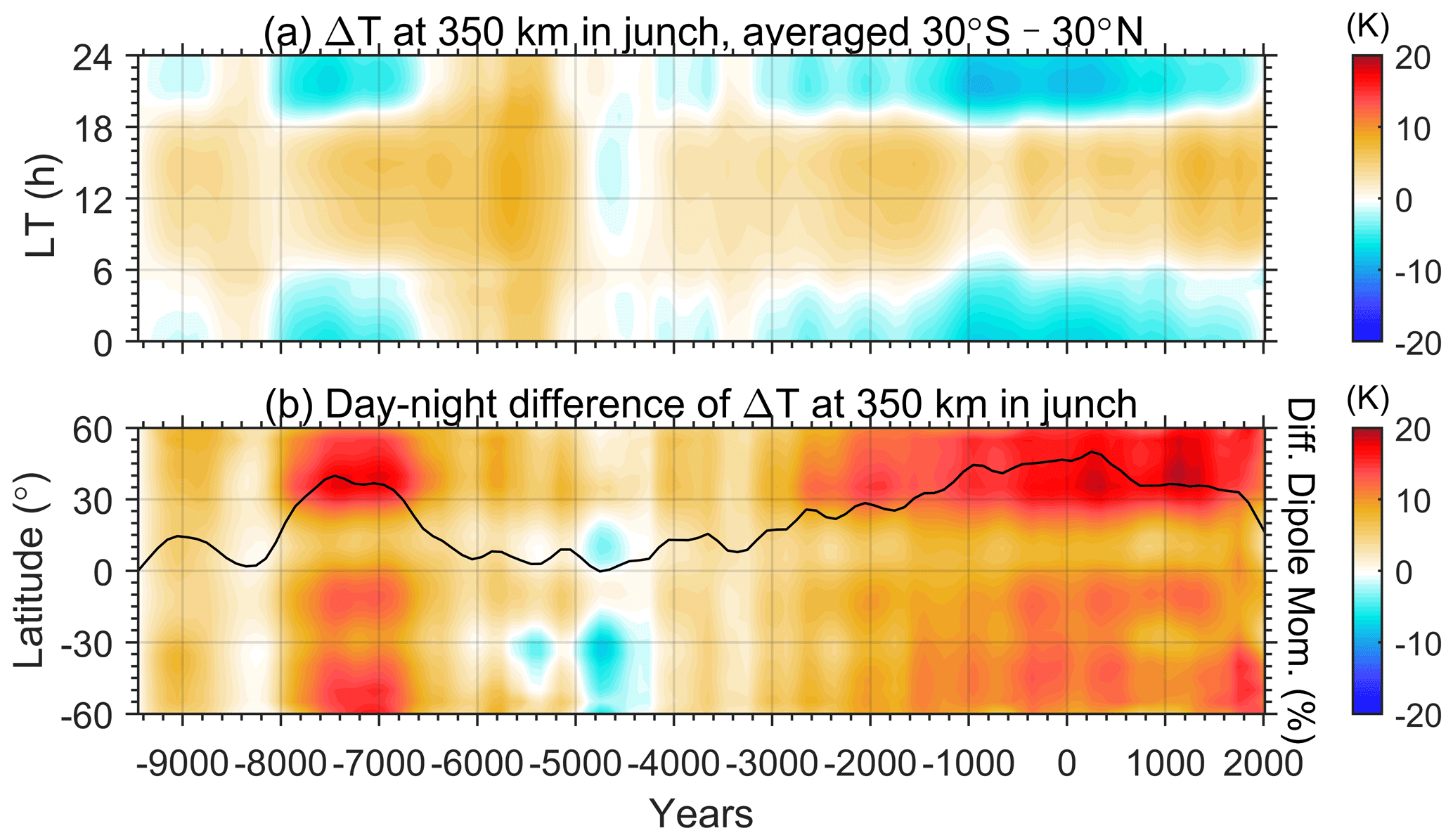
Figure 6 (a) Local-time (LT) variation of the zonal mean temperature changes at low latitudes (30^∘ S–30^∘ N) caused by the secular variation of geomagnetic fields at 350 km in March during the Holocene. (b) Latitudinal variation of day–night differences in the zonal mean temperature during March plotted versus year and with respect to the beginning of the simulation. The daytime and nighttime are corresponding to 10:00–14:00 and 22:00–02:00 LT, respectively. Relative change of the geomagnetic dipole moment is plotted in the solid black line in plot (b).

Figure 7 Same as Fig. 6, but for the case of June.

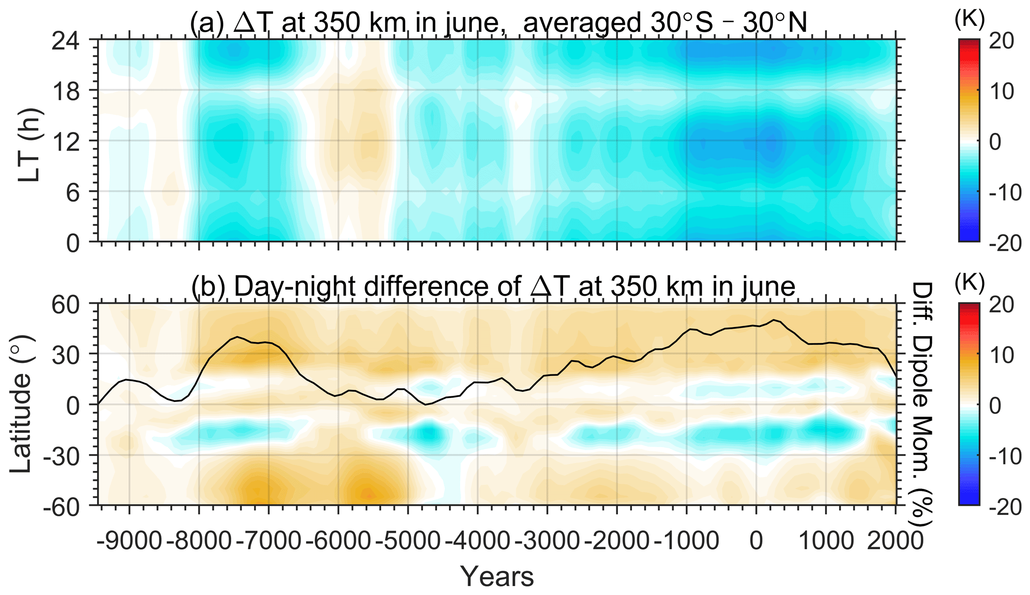
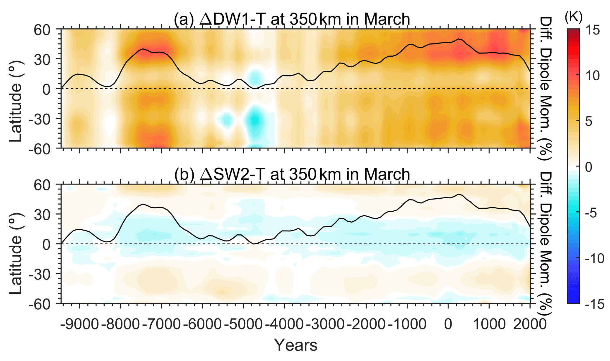
Figure 8 Time evolution of the differences in the amplitude of (a) DW1 and (b) SW2 with respect to the beginning of the simulation.

In addition, Fig. 5b and d shows that the geomagnetic variation during the period 1945–2015 induced different temperature responses during the daytime/nighttime at middle and low latitudes. This local-time-dependent effect is further examined in Figs. 6 and 7 for the month of March and June, respectively. Figure 6a illustrates the local-time dependence of temperature changes due to the geomagnetic variation with respect to the beginning year of 9455 BC, when the dipole moment of the geomagnetic field underwent a minimum period. During the daytime, the average temperature at low latitude was generally higher than in 9455 BC for most of the time, except for 4900 BC and 4700 BC. The changed magnitude varied from −2 to 9 K. In contrast, the night-time temperature change is negative compared to 9455 BC since 3100 BC and ranges from −7 to +6 K before 3100 BC. We then deduced the day–night differences in the temperature response at middle and low latitudes and illustrated them in comparison with the strength of the geomagnetic dipole moment in Fig. 6b. The results show an obviously positive correlation between the day–night differences and the geomagnetic dipole moment, indicating that a stronger geomagnetic dipole moment would induce larger day–night temperature differences in the thermosphere at middle to low latitudes in March, thereby exacerbating the prevailing day-to-night flow. During the whole simulation period in the Holocene, the day–night difference in temperature caused by the geomagnetic variation can vary up to ∼15–20 K. The fluctuation magnitude is about 5 % relative to the typical day–night temperature difference in the thermosphere of 300–400 K. Meanwhile, the geomagnetic dipole moment varies more than 40 %. As for the case of June, the positive correlation is not valid for all latitudes and becomes more complicated. As the dipole moment increases, the average temperature at low latitudes decreases for both daytime and nighttime. The change in the day–night temperature difference is weaker than that in March. Around the Equator and in the southern middle latitudes, the day–night difference in temperature decreases while the geomagnetic dipole moment increases, such as during 8000–6600 BC and 2600 BC–AD 1600.

As mentioned above, the day-time temperature responses in the thermosphere differed from that of the nighttime due to the geomagnetic variation, suggesting that the tidal response should also be affected, especially during March. Figure 8 then examines the thermospheric tidal response to the geomagnetic variation during the Holocene in the CR2 simulation, including the diurnal and semidiurnal migrating tides in temperature (DW1−T and SW2−T). These two major tidal components respond differently to the geomagnetic variation. The strength of DW1−T is positively correlated with the geomagnetic dipole moment. When the dipole moment intensity becomes ∼40 % larger than at the beginning of the simulation, the amplitude of DW1−T increases correspondingly by ∼10 K. However, the SW2−T around the Equator is negatively correlated to the geomagnetic dipole moment, while at middle latitudes it is positively correlated. The strength of SW2−T response to the geomagnetic variation is much smaller than that of DW1−T and ranges within $\sim \pm \mathrm{2}$ K throughout the simulation period in the Holocene. Figure 9 further diagnoses the relationship between the thermospheric migrating tides and the geomagnetic dipole moment for different thermospheric altitudes versus latitudes. A linear regression between the tidal amplitude and geomagnetic dipole moment is calculated. Figure 9a and b illustrates the estimated coefficient for the linear regression in the altitude–latitude plane, with regions where the absolute value of the correlation coefficient is less than 0.6 being masked. The results show that as the geomagnetic dipole moment increases per 10²² A m², the thermospheric DW1−T in March would enhance by 1–3 K, with two maximums around ±30–40^∘. The response of SW2−T is much smaller and insignificant. At the Equator, the increase in geomagnetic dipole moment by 10²² A m² would lessen the SW2−T amplitude merely by ∼0.3 K. A slight enhancement of SW2−T due to the increase in geomagnetic dipole moment could be found in the upper thermosphere at middle latitudes, while the growth rate is only ∼0.4 K/10²² A m².

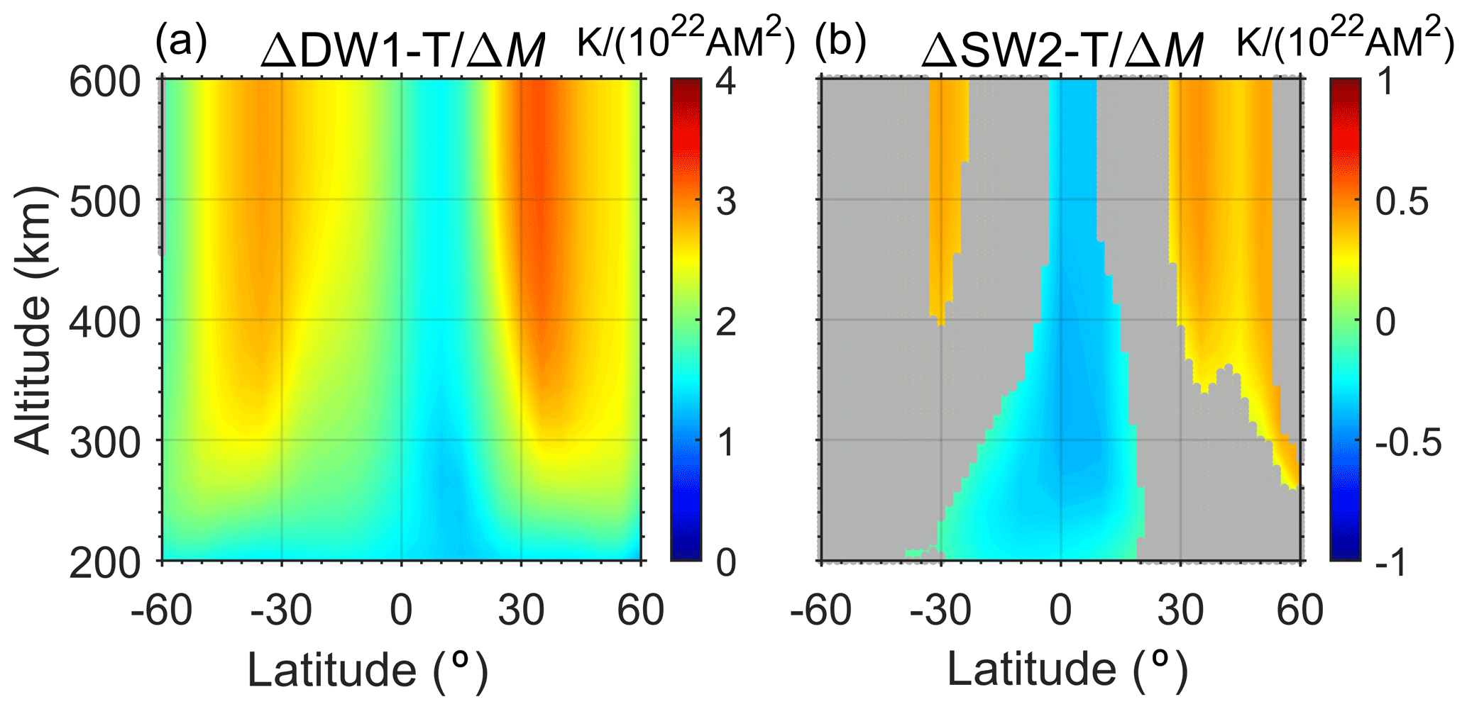
Figure 9 Coefficient estimates for the linear regression of (a) DW1−T and (b) SW2−T amplitudes on the geomagnetic dipole moment. The shaded gray area indicates where the absolute values of correlation coefficients are less than 0.6.

4 Discussion

In this paper, two control runs, CR1 and CR2, were conducted to examine the response of thermospheric dynamics to long-term changes in CO₂ and geomagnetic field during the last 12 000 years of the Holocene. The CO₂ effect was revealed as an enhancement of the general circulation with increasing CO₂ levels (Figs. 1 and 2), which agreed with the result of Liu et al. (2020). Rind et al. (1990) also found that an increase in CO₂ similarly enhanced the mesospheric circulation. Both of them suggested that the increased eddy forcing and gravity waves (GWs) should play an important role. However, the GCITEM-IGGCAS model does not involve a parameterization scheme for GWs because the GWs mainly affect the mean flow in the mesosphere rather than in the thermosphere. Therefore, the changes in the circulation caused by CO₂ variations in our results cannot be attributed to GWs. The interpretation by Kogure et al. (2022) should be responsible for the fact that the changes in ion drag, molecular viscosity, and meridional pressure gradient forces are in the combined modulation. An interesting founding is that the CO₂ increase does not linearly accelerate the circulation and tends to be “saturated”, as shown in Fig. 3. The plausible explanation is that the molecular viscosity is non-linearly related to the temperature. As for the tidal response to the CO₂ effect, the DW1 amplitude is positively correlated with CO₂ variation (Fig. 4). A reasonable deduction is that the decreased viscosity due to the enhanced CO₂ cooling should be less likely to dissipate tidal propagation from below. The latitudinal structure of the DW1 response to CO₂ differs from that of Liu et al. (2020), partly because their results mixed the influences of changes in tidal sources from below, whereas our results reflected the internal thermospheric responses. In addition, this paper only considered the geomagnetically quiet condition, while the efficiency of CO₂ forcing somewhat differs under low and high geomagnetic activity conditions according to GAIA simulations by Liu et al. (2021).

Figure 5 illustrated an asymmetric response in circulation to the geomagnetic variation. The change in neutral winds was larger in the hemisphere with a more distant geomagnetic pole shift. Given that the variation in the dipole component of the geomagnetic field is hemispherically symmetrical, it could logically be inferred that the hemisphere difference in circulation is contributed by the variation of the non-dipole component. The neutral temperature change due to geomagnetic variation has a similar pattern to the ion temperature in Cnossen (2014), which is also manifested to decrease around the day-time equatorial ionization anomaly (EIA) peaks. A possible causal linkage could be proposed that the geomagnetic variation affected the equatorial plasma drift velocity and then redistributed the electron density around the EIA region. As the electron density becomes large/small, the electron temperature changed conversely. The ion temperature change then should be more or less related to the electron temperature change. Generally, the smaller strength of the geomagnetic fields would induce stronger equatorial vertical drift ($E\times B/B^{\mathrm{2}}$) and thus increase the electron density at the EIA peaks, and Yue et al. (2022) confirmed such a relationship. During the nighttime, the equatorial drift tended to be downward and the EIA structure disappeared in general. So, the above-discussed causality is not valid, and the night-time neutral temperature response should be different. The increased Joule heating related to the weakening of the geomagnetic field might be responsible. Hence, the geomagnetic variation would redistribute the temperature in the daytime and nighttime differently (Fig. 6), then causing the day–night difference in Figs. 6 and 7. The seasonal dependence of the day–night difference in temperature response to the geomagnetic variation is still puzzling and needs further explanation in the future. The temperature redistribution due to geomagnetic variation then causes the tidal responses in Figs. 8 and 9. At middle latitudes, both DW1 and SW2 manifest to be positively correlated to the dipole moment, partly because the cooler thermosphere caused by the strengthening geomagnetic field (Cai et al., 2023) modulated the tidal propagation from below. At the low latitudes, the effect from E×B drift at daytime becomes important as aforementioned, therefore different from that in middle latitudes.

As a tentative investigation of the long-term change of thermospheric dynamics during ∼12 000 years, this paper still has some limitations and flaws, and one of them is the fixed lower boundary. In the present work, the migrating tides at the lower boundary (90 km) are set to be unvaried regardless of simulating different periods in the Holocene. To our knowledge, the long-term trend around the mesopause is still debated, and the understanding changed from no trend to a mild negative trend in general (Beig et al., 2003; Huang et al., 2014; Laštovička, 2017). This is partly because the temperature trends at these heights are sensitive to the changes in stratospheric ozone concentration (Lübken et al., 2013). A whole-atmosphere simulation performed by Solomon et al. (2018) also indicated there are very weak trends in the mesopause region. Hence, the perpetual lower boundary should be a conservative and compromised treatment, additionally considering that little evidence has been provided on how the atmospheric tides change during such a long-term historical time. Besides, the fixed lower boundary inferred that the tidal source from the lower atmosphere is constrained to be unvaried, so our results mainly describe the effect of propagation conditions and local excitation on the long-term dynamics change in the thermosphere. In the next step, simulation based on a whole-atmosphere climate model, like the WACCM-X (Liu et al., 2018) and GAIA (Jin et al., 2011), should give a much more realistic scenario of the long-term change in the thermospheric dynamics, nevertheless, the computation cost will increase substantially.

In addition, the empirical model describing the high-latitude input, Weimer-96, is based on modern satellite measurements. Although the geomagnetic intensity variation has not been taken into consideration by the model, the effect of the geomagnetic tilted angle has been included. The drift of magnetic poles and aurora region is thus considered, given that the Weimer-96 is based on a magnetic coordinate. The intensity of the geomagnetic field is examined as influencing the magnetosphere configuration and thus is expected to affect the energy input to the high-latitude thermosphere (Zhong et al., 2014; Cnossen et al., 2012). Vogt et al. (2009) summarized the potential impact of the geomagnetic field variation on the geospace by modulating the shielding of the energetic charged particles. During the simulated period, the dipole moment (M) is in the 6×10²²–1×10²³ A m² range. As the sine of polar cap size (θ) is generally proportional to $M^{-\mathrm{1}/\mathrm{6}}$, a rough estimation deduces that θ would change by ∼3^∘, within latitudinal resolution (5^∘) in the model. Theoretical scaling about cross-polar cap potential (Φ), $\mathrm{\Phi }\propto M^{\mathrm{1}/\mathrm{3}}$, infers that the Φ should varied from 18 to 21 kV during the Holocene if we set the Φ as 20 kV at the present era. Comparing a typical geomagnetically disturbed condition that Φ is ∼80 kV for Kp=4, the relative change in Φ above is quite small. Cnossen (2014) also declared that the magnetosphere–ionosphere coupling is only significant during the disturbed conditions. Given that our simulation is perpetually geomagnetically quiescent, the impact of geomagnetic variation on the high-latitude energy input should be limited.

In this work, the CO₂ and geomagnetic fields were regarded as two independent external drivings to the simulation regardless of their interaction, although whether the interaction exists is still controversial. Zhou et al. (2021) proposed that the decrease in geomagnetic intensity would redistribute the CO₂ in the upper atmosphere using the whole-atmosphere simulation. Their investigation suggested that the increased ionospheric conductivities due to the weakened geomagnetic intensity would induce much more Joule heating to warm the high-latitude lower thermosphere, which then should enhance the upwelling flow and bring rich CO₂ from below. This result is based on the physical fact that the CO₂ distribution becomes deviated from the well-mixed equilibrium above the mesopause (∼80–90 km), and the timescale of eddy diffusion becomes much larger in the upper atmosphere (Beagley et al., 2010; Rezac et al., 2015), so that the dynamical processes could modulate the CO₂ distribution. However, until now, little observational evidence has been proposed to support the possible link between CO₂ and geomagnetic fields. A simulation project conducted by the whole-atmosphere model in the next step could provide more information.

Responses of the non-migrating tides to the variation of CO₂ and geomagnetic fields were not considered in this paper. The eastward propagating diurnal tides with a zonal wavenumber of 3 (DE3) should not be very sensitive to the CO₂ change, according to the discussion by Liu et al. (2020). This result was expected, as the longitudinal variation of CO₂ concentration is generally not obvious. On the other hand, geomagnetic fields crucially influence the non-migrating tidal propagation in the upper atmosphere, through the electro-dynamo or parallel-line transport. For example, Jiang et al. (2018) revealed that DE3 tide can induce the longitudinal wavenumber-3 (WN3) structure rather than the should-be WN4 structure through the electro-dynamical coupling with the geomagnetic field. Zhang et al. (2020) proposed that the significant role of parallel-line transport alters the interhemispheric symmetry as the enhanced planetary waves upward propagated during the 2009 sudden stratosphere warming (SSW) event. As the realistic geomagnetic field is much more complicated than the dipole or tilted dipole, a given non-migrating tide propagating into the thermosphere would broaden the spectra of wavenumbers. Yue et al. (2013) found that there were complicated longitudinal structures rather than simply the WN3 as the quasi 2 d wave with westward zonal wavenumber 3 propagating into the upper atmosphere. In this future work, the non-migrating tidal response to the long-term variation will be worth studying.

5 Conclusions

This paper diagnosed the long-term changes in the thermospheric dynamics caused by the secular variation of CO₂ emissions and geomagnetic field during the Holocene, using the global coupled thermosphere–ionosphere model, GCITEM-IGGCAS. Two sets of long-term time-slice simulations covering ∼12 000 years were performed by independently controlling the CO₂ level and the configuration of geomagnetic fields, both under the perpetual condition of solar minimum and geomagnetic quiescence. The corresponding changes in the circulation and major solar tides in the thermosphere were then analyzed, and the main results were summarized as follows:

1. The CO₂ increase/decrease generally strengthened/weakened the general circulation in the thermosphere, and notably the circulation has intensified dramatically with the steep increase in CO₂ since the industrial revolution. The circulation increase due to the CO₂ variation was found to grow non-linearly, which is expected to be caused by the non-linear relationship between temperature and molecular viscosity.

2. The amplitude of the diurnal migrating tide in the thermosphere will strengthen as the CO₂ increases throughout the Holocene because the increased CO₂ cooling provides a plausible condition for tidal propagation.

3. Secular variations of the geomagnetic field have a regional impact on the thermospheric circulation, which is particularly pronounced at high latitudes and around the dusk sector. The prominent hemispheric differences in the thermospheric circulation response infer a crucial role of the geomagnetic non-dipole component.

4. Geomagnetic variations also redistribute neutral temperature at middle and low latitudes and leads to different responses in the daytime and nighttime, which then influence the thermospheric dynamics.

5. The geomagnetic dipole moment is highly correlated with DW1 tidal amplitude at middle and low latitudes during March, and an enhancement of 1×10²² A m² will cause an increase in ∼1–3 K of DW1−T in the thermosphere.