Simulated long-term evolution of the thermosphere during the Holocene – Part 1: Neutral density and temperature

In the previous work of Yue et al. (2022), the ionospheric evolution during the Holocene (9455 BC to 2015 AD) was comprehensively and carefully investigated for the first time using the Global Coupled Ionosphere-Thermosphere-Electrodynamics Model developed at the Institute of Geology and Geophysics, Chinese Academy of Sciences (GCITEM-IGGCAS), driven by realistic geomagnetic fields, CO₂ levels, and solar activity derived from ancient media records and modern measurements. In this study, we further quantify the effects of the three drivers on thermospheric neutral density and temperature variations during the Holocene. We find that the oscillations of solar activity contribute more than 80 % of the thermospheric variability, while either CO₂ or the geomagnetic field contributes less than 10 %. The effect of CO₂ on the global mean neutral density and temperature is comparable to that of the geomagnetic field throughout the Holocene but is more significant after 1800 AD. In addition, thermospheric density and temperature show approximately linear variations with the dipole moment of the geomagnetic field, CO₂, and F10.7, with only the linear growth rate associated with the geomagnetic field varying significantly in universal time and latitude. The increasing dipole moment and CO₂ cool and contract the thermosphere, while solar activity has the opposite effect. The higher the altitude, the greater the influence of the three factors on the thermosphere. Different factors produce different seasonal variations in thermosphere changes. Furthermore, we predict that a 400 ppm increase in CO₂ will result in a 50 %–70 % and 84–114 K reduction in global mean neutral density and temperature, respectively, which should directly affect the orbit and lifetime of spacecraft and space debris.

1 Introduction

Global glaciers have been melting in the recent century due to climate warming, and this melting has been accelerating in the last 20 years, leading to rising sea levels and elevating natural disasters (Hugonnet et al., 2021; Zemp et al., 2019). The main cause of climate warming is the use of fossil fuels as a source of anthropogenic greenhouse gases (Tollefson, 2021). The simulations of Roble and Dickinson (1989) show that the increase in greenhouse gases warms the troposphere but cools the thermosphere. The long-term trend studies in subsequent decades largely support this consensus (Laštovička, 2009; Laštovička et al., 2006, 2008). Tropospheric warming seriously affects human life, while changes in the thermosphere affect various human-launched satellites, space stations, and spacecraft, such as the SpaceX Starlink satellite destruction event on 4 February 2022 (Dang et al., 2022; Lin et al., 2022), and are therefore also relevant to human life. The current understanding of the thermosphere is based on modern satellite observations over the last ∼ 70 years. The energy sources driving the variability of the thermosphere include mainly solar irradiance and geomagnetic activity generated by the interaction between the solar wind and the Earth's magnetic field (Knipp et al., 2004). These two energy sources are responsible for thermospheric temporal variations on timescales ranging from minutes to decades. On longer timescales, however, the effects of greenhouse gases and the geomagnetic field must be taken into account (Laštovička et al., 2006). Several review papers have summarized the knowledge of thermospheric variations and their driving mechanisms (Laštovička, 2017; Laštovička et al., 2012; Qian et al., 2011; Qian and Solomon, 2012).

Long-term trends of neutral density at different altitudes between 200 and 600 km have been extensively investigated using satellite orbit measurements since the 1960s (Emmert, 2015; Emmert et al., 2004, 2008; Saunders et al., 2011; Marcos et al., 2005; Keating et al., 2000). These studies suggested that the trend is mainly attributed to a dramatic increase in anthropogenic greenhouse gases and becomes stronger with increasing altitude. A summary of the trends derived from satellite orbit data can be found in Emmert (2015) and Solomon et al. (2018). Overall, the observed long-term trend of the thermospheric neutral density at 400 km ranges from −2 % to −5 % per decade. These observed characteristics are qualitatively consistent with the model-predicted effects of increasing CO₂ concentration (Qian et al., 2006; Roble and Dickinson, 1989; Solomon et al., 2015). The effect of geomagnetic field strength and configuration on the thermosphere has also been paid enormous attention from observations and simulations (A et al., 2012; Cnossen, 2014, 2022; Cnossen and Maute, 2020; Cnossen et al., 2012, 2011; Förster and Cnossen, 2013). However, none of these effects is as significant as the effect of solar activity on the thermosphere. The amplitude of the solar-driven variation increases with height by a factor of 2 for temperature and an order of magnitude for density in the upper thermosphere (Qian and Solomon, 2012; Solomon et al., 2019). Overall, these observations and simulations of the thermosphere are limited to the recent 100 years, while the “ancient” thermosphere has never been investigated on longer timescales such as during the Holocene. Therefore, we propose reconstructing the paleo-thermosphere since the Holocene using the first-principle numerical model driven by these indices, including solar activity derived from tree rings (Solanki et al., 2004), paleo-geomagnetic field models (Korte et al., 2011), and greenhouse gas concentrations derived from polar ice cores (Lüthi et al., 2008). Based on the reconstructed simulations, we can understand the evolution of the thermosphere over 10 000 years and the effects of changes in the geomagnetic field, CO₂, and solar activity on the thermosphere, which can provide a foundation for the future effect of climate change on human life.

The rest of the paper is organized as follows. Section 2 will briefly describe the numerical model and driving parameters used in this study. Section 3 will show the simulation results and discuss them. Finally, we draw conclusions in Sect. 4.

2 Methodology

This study will use the Global Coupled Ionosphere-Thermosphere-Electrodynamics Model developed at the Institute of Geology and Geophysics, Chinese Academy of Sciences (GCITEM-IGGCAS) (Ren et al., 2009), which is the same as that used by Yue et al. (2022). This model self-consistently solves the energy, momentum, and continuity equations of neutrals and ions in altitude coordinates rather than pressure-level coordinates between 90 and 600 km and solves the electrodynamic equations using magnetic-apex coordinates (Richmond, 1995) based on provided spherical harmonic coefficients of any dipole-dominated geomagnetic field, such as the International Geomagnetic Reference Field (IGRF) model (Alken et al., 2021). This model has a good performance that has been confirmed by several ionospheric and thermospheric weather and climate simulations (Yue et al., 2022; Zhou et al., 2022; Ren et al., 2011, 2020, 2010). To remove the effects of initial conditions, each simulation is run for an interval of 15 d, and the final-day results are used for further analysis.

Three drivers associated with geomagnetic field, CO₂ level, and solar activity during the Holocene, 9455 BC to 2015 AD, are used to drive the GCITEM-IGGCAS. These drivers have been summarized in Fig. 1 of Yue et al. (2022). The geomagnetic field is CALS10k.2 (Constable et al., 2016) for the period 9455 BC to 1900 AD and the IGRF after 1900. The geomagnetic field has undergone complex and nonlinear changes during the Holocene, with a dipole moment variation of ∼ 40 %, much larger than the ∼ 7 % variation since 1900. The CO₂ concentration evolution is derived from Antarctica Vostok and EPICA Dome C ice cores (Lüthi et al., 2008), Antarctica Law Dome ice cores (Macfarling Meure et al., 2006), and direct atmospheric measurement at Mauna Loa Observatory, Hawaii (Keeling et al., 1995). The CO₂ concentration increases roughly linearly from 250 ppm (parts per million) around 10 000 BC to 402 ppm around 2015 AD, with a major increase occurring after 1800. The F10.7 index evolution converted from the tree-ring-derived sunspot number (SSN) (Solanki et al., 2004) and the group SSN (Hoyt and Schatten, 1998) and modern instrument measurement (Tapping, 2013), which reveals the long-term oscillations in solar activity with relatively high solar activity around 9000 BC and 1960 AD. A detailed description of the three drivers can be found in Yue et al. (2022).

Figure 1 Time evolution of the global mean neutral density and temperature at 400 km in the March equinox (top row). The other rows are global plots of CR4-simulated neutral density (left column) and temperature (right column) for four selected years at 19:00 UT during the March equinox. The corresponding model drivers are also given in the white text, and “DM” means the dipole moment of the geomagnetic field. The gray line in each color plot marks the inclination equator for the corresponding year.

In this simulation, four control runs (CR1–CR4) have been implemented, which is the same as Yue et al. (2022) (summarized in their Table 1). CR1 is used to identify the effect of geomagnetic field variation on thermospheric evolution. CR2 is used to reveal the effect of CO₂. CR3 is used to diagnose the combined effect of geomagnetic field and CO₂. CR4 is used to determine the combined effects of geomagnetic field variation, solar activity, and CO₂. In addition, the combined analysis of the simulations of CR3 and CR4 allows one to discern the effect of solar activity.

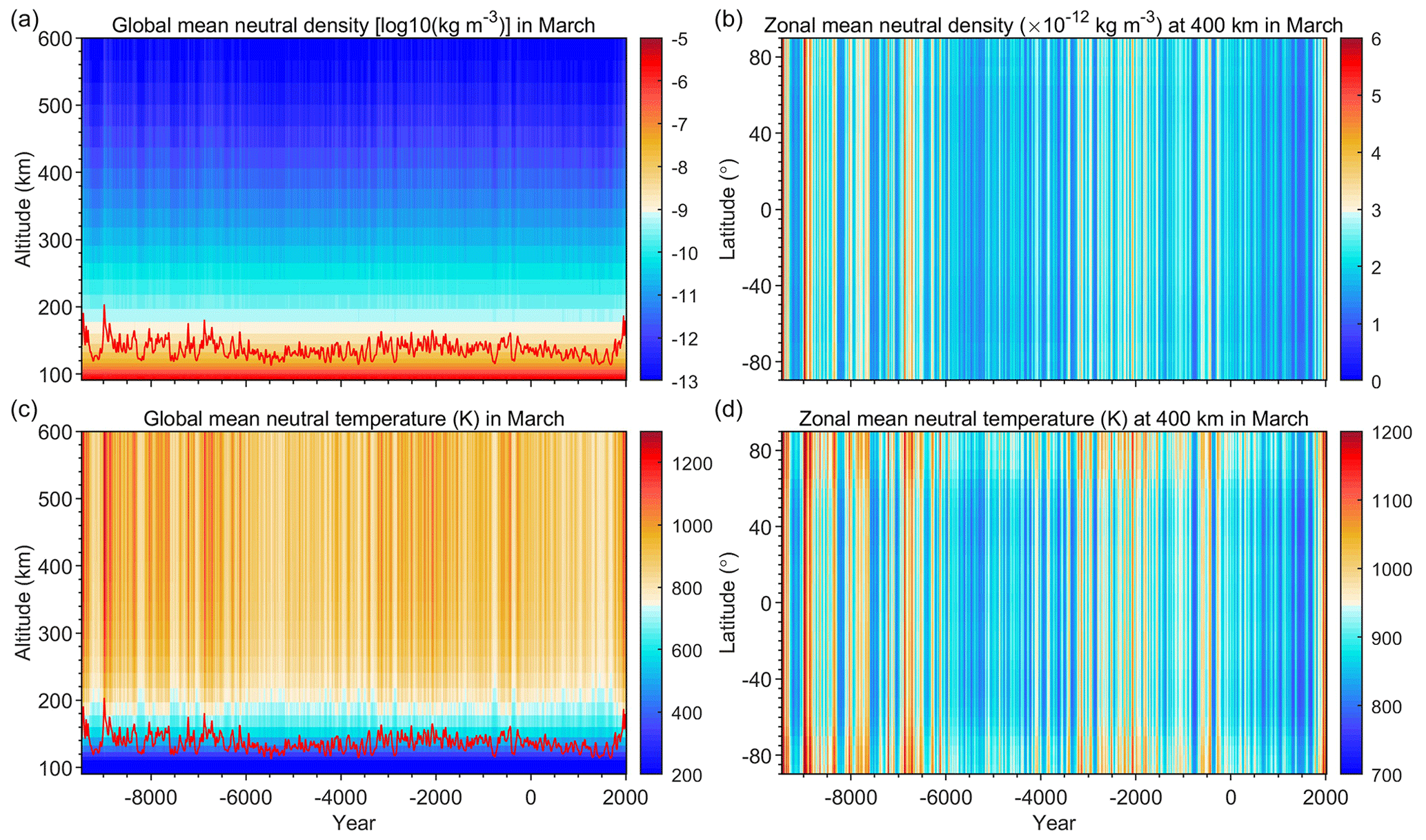
Figure 2 Global mean (all UTs and grids) neutral density and temperature profiles versus years (a, c) and zonal mean (all longitudes and UTs) neutral density and temperature at 400 km as a function of latitude and years (b, d) in the March equinox from CR4 simulations. Note that the color scale is different for each plot. The red line in the left column represents the relative change in the F10.7 index over the Holocene.

3 Results and discussions

3.1 Thermosphere evolution during the Holocene

Figure 1 shows the overall evolution of the CR4-simulated thermospheric neutral density and temperature in the March equinox during the Holocene. The top row displays the time evolution of the global mean neutral density and temperature at 400 km, and the other rows give the global map of neutral density and temperature at 400 km at universal time (UT) 19:00 for the considered four years (9005 BC, 7635 BC, 3015 BC, and 2005 AD). The white text of the global map in the left column of Fig. 1 gives the corresponding F10.7 index, CO₂ level, and dipole moment of the geomagnetic field. It is clear that the global mean neutral density and temperature are mainly controlled by solar activity as they show essentially the same temporal evolution and oscillation as solar activity. The higher the solar activity, the larger the neutral density and temperature in general, with a relatively larger value around 9000 BC and 1960 AD. The global distribution of neutral density and temperature shows a remarkable feature during the dayside with two peaks on either side of the geomagnetic inclination equator, the so-called equatorial mass anomaly (EMA), like the equatorial ionization anomaly (EIA) in the ionosphere (Appleton, 1946; Balan et al., 2018), indicating a strong coupling between the thermosphere and ionosphere modulated by the geomagnetic field at low and middle latitudes (Hedin and Mayr, 1973; Liu et al., 2005, 2007; Raghavarao et al., 1993, 1991). Comparing the simulations for the considered four years can basically reveal the influence of CO₂, geomagnetic field, and solar activity on the evolution of the thermosphere. The F10.7 index and CO₂ level used to drive GCITEM-IGGCAS are similar in 9005 and 7635 BC, except that the dipole moment is about 20 % larger in 7635 BC than in 9005 BC. It is clear that the simulated neutral density and temperature for these two years are not significantly different in global distribution pattern and magnitude, which indicates that the ∼ 20 % change in dipole moment has a weak effect on the thermosphere at 400 km altitude. Comparing the simulations of 9005 and 3015 BC reveals that a ∼ 25 % reduction in the F10.7 index leads to a ∼ 50 % decrease in neutral density and a ∼ 170 K decrease in neutral temperature. Furthermore, the cooling effect of CO₂ on the thermosphere can be found by comparing the simulations of 9005 BC and 2005 AD. An increase of 110 ppm (∼ 40 %) in CO₂ concentration causes a temperature reduction of ∼ 40 K and a density reduction of ∼ 21 %. In addition, we also checked the simulations at other UTs and during the June solstice as well. In summary, the thermosphere is primarily controlled by solar activity, with secondary controlled factors being CO₂ and the geomagnetic field.

Figure 2 shows the global mean for all UTs and grids of the neutral density and temperature as a function of altitude and year (left column) and the zonal mean neutral density and temperature versus latitude and year at 400 km (right column) in the March equinox during the Holocene. According to Afraimovich et al. (2008), a latitude-dependent area-weighting factor was used in the calculation of the global mean to make it more representative. As shown in Fig. 2, both the global mean and zonal mean display significant oscillations throughout the whole Holocene, which is consistent with the oscillations of the solar activity whose relative change was marked by the red lines in the left column. When F10.7 reaches its relatively higher value before 8000 BC and in the recent century, a larger value of neutral density and temperature also appears. This feature is not clearly visible in the altitude profile of the global mean of neutral density (Fig. 2a) due to the span of about 10 orders of magnitude. However, this does not affect the conclusion, after all, that the fixed height of the zonal mean is more revealing of this feature. Furthermore, the thermospheric neutral density and temperature also show significant long-term decreases from 6000 to 3500 BC and the most famous grand solar minimum (Usoskin et al., 2007), the Maunder minimum between 1645 and 1715 (Eddy, 1976). Only a weak latitudinal variation can be seen in the zonal mean neutral temperature in the March equinox.

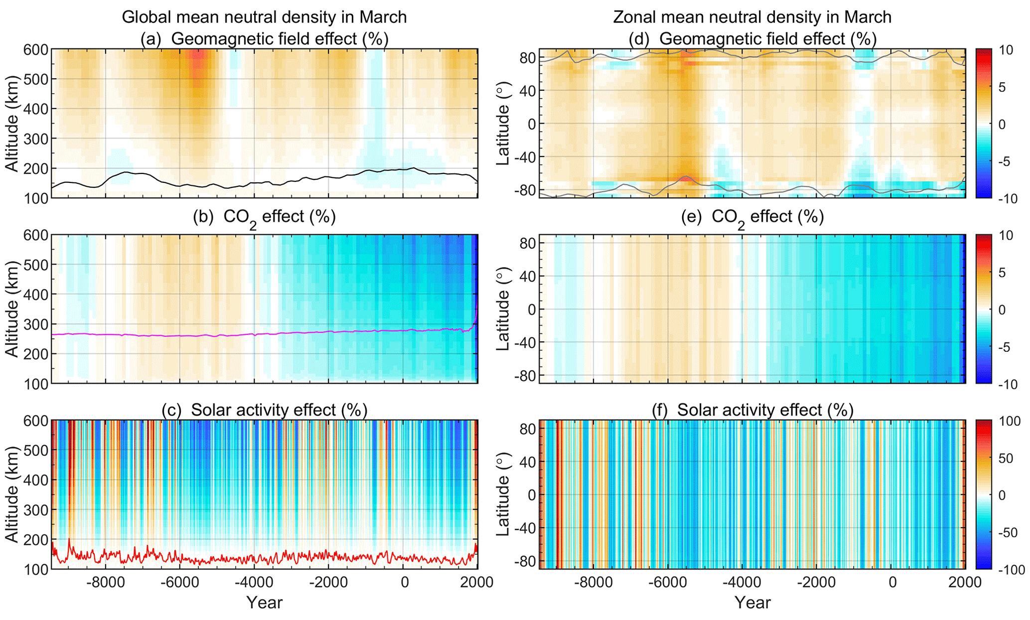
Figure 3 The global mean (all grids and UT) neutral density profiles deviate from the beginning year of the simulation due to changes in the geomagnetic field (a, CR1), CO₂ (b, CR2), and solar activity (c, CR4–CR3) as a function of altitude and years. Panels (d), (e), and (f) show the same pattern as the left column except that the zonal mean neutral density (all longitudes and UTs) at 400 km is shown. The gray lines in panel (d) mark the latitude of the north and south magnetic poles for the corresponding year. The black, magenta, and red lines in the left column represent the relative changes in the dipole moment, CO₂, and F10.7 index, respectively, during the Holocene.

Figure 4 The same as Fig. 3 but for the neutral temperature.

3.2 The effects of the three drivers on the evolution of thermospheric neutral density and temperature

In this section, the changes in thermospheric neutral density and temperature caused by the geomagnetic field, CO₂, and solar activity will be diagnosed by subtracting the beginning year (9455 BC) of the simulations, as shown in Figs. 3–5 for the results of the global mean and zonal mean.

Figure 3 shows the global mean neutral density profile variations in percentage caused by the three drivers in the left column. The black, magenta, and red lines represent the relative changes in the diploe moment, CO₂, and F10.7 index, respectively, during the Holocene. In general, the higher the altitude, the larger the effect of the three drivers on the neutral density, because the neutral density decreases exponentially with altitude, causing all the effects to be amplified at higher altitudes. For the effect of the geomagnetic field, its nonlinear variation causes a nonlinear change in the neutral density, and a decrease in its intensity represented by the weakening of the dipole moment (around 5500 BC) generally leads to an increase in the neutral density. In addition, an increase in the dipole moment would make the neutral density increase weaker, which might be related to the decrease in Joule heating due to the strong dipole moment (Cnossen et al., 2012, 2011; Wang et al., 2017; Glassmeier et al., 2004). When the dipole moment increases beyond ∼ 3 × 10²² Am² (at ∼ 7500 BC and from ∼ 1500 BC to ∼ 1000 AD), the density will decrease in turn between 150 and 250 km. For the effect of CO₂, the neutral density decreases during the increase phase of the CO₂ level (before ∼ 8000 and after ∼ 4000 BC). This is because greenhouse gases can cool and contract the thermosphere (Qian et al., 2011), as shown in Fig. 4 for temperature reduction. In turn, when CO₂ decreases between ∼ 8000 and ∼ 4000 BC, the thermosphere neutral density increases. It is worth noting that the effect of CO₂ has been more significant since 1800 AD due to the much larger growth rate of CO₂. For the effect of solar activity, the overall change in neutral density due to solar activity is more than 10 times larger than that of CO₂ and the geomagnetic field, so it is the dominant factor in neutral density change. The neutral density has increased by more than 100 % in the recent century and around 9000 BC, which corresponds to relatively greater solar activity. The right column of Fig. 3 shows the zonal mean results at 400 km. The gray lines in panel d mark the latitude of the north and south magnetic poles for the corresponding year. The effects of the three drivers on the temporal evolution of the neutral density at all latitudes are similar to those characterized in the left column, with no significant latitude variations in the effects of CO₂ and solar activity and a weak latitude variation in the effect of the geomagnetic field, which is stronger at high latitudes. The region with greater geomagnetic field effects corresponds exactly to the magnetic pole locations, such as the south magnetic pole at ∼ 64^∘ around 5500 BC, implying the importance of the magnetic pole locations and further supporting the contribution of Joule heating in the polar region.

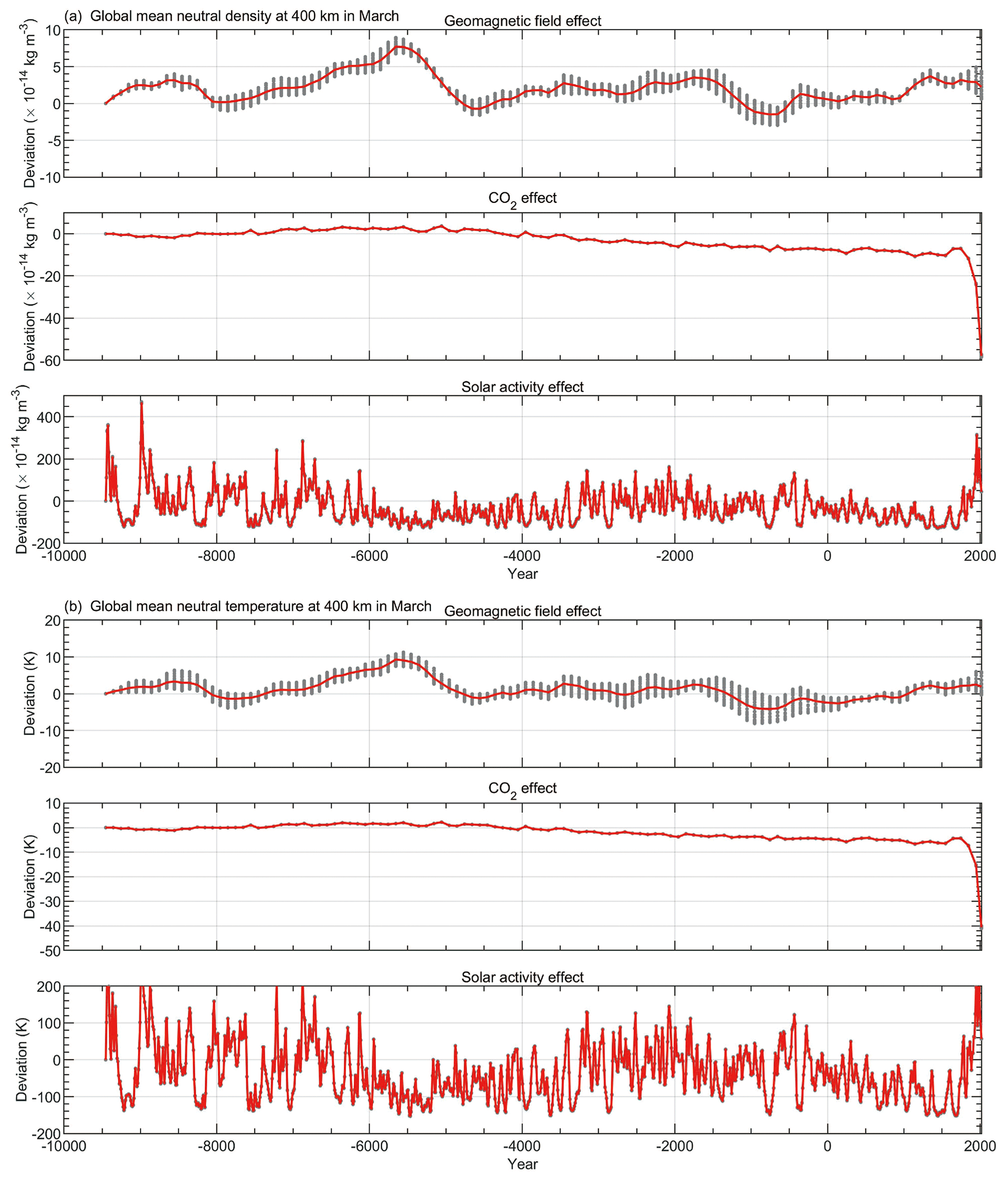
Figure 5 Global mean (red line) neutral density (a) and temperature (b) deviations with respect to the beginning of the simulation versus years at 400 km during the March equinox due to the geomagnetic field variation (CR1), the CO₂ variation (CR2), and the solar activity variation (CR4–CR3). The gray dots represent different UT results.

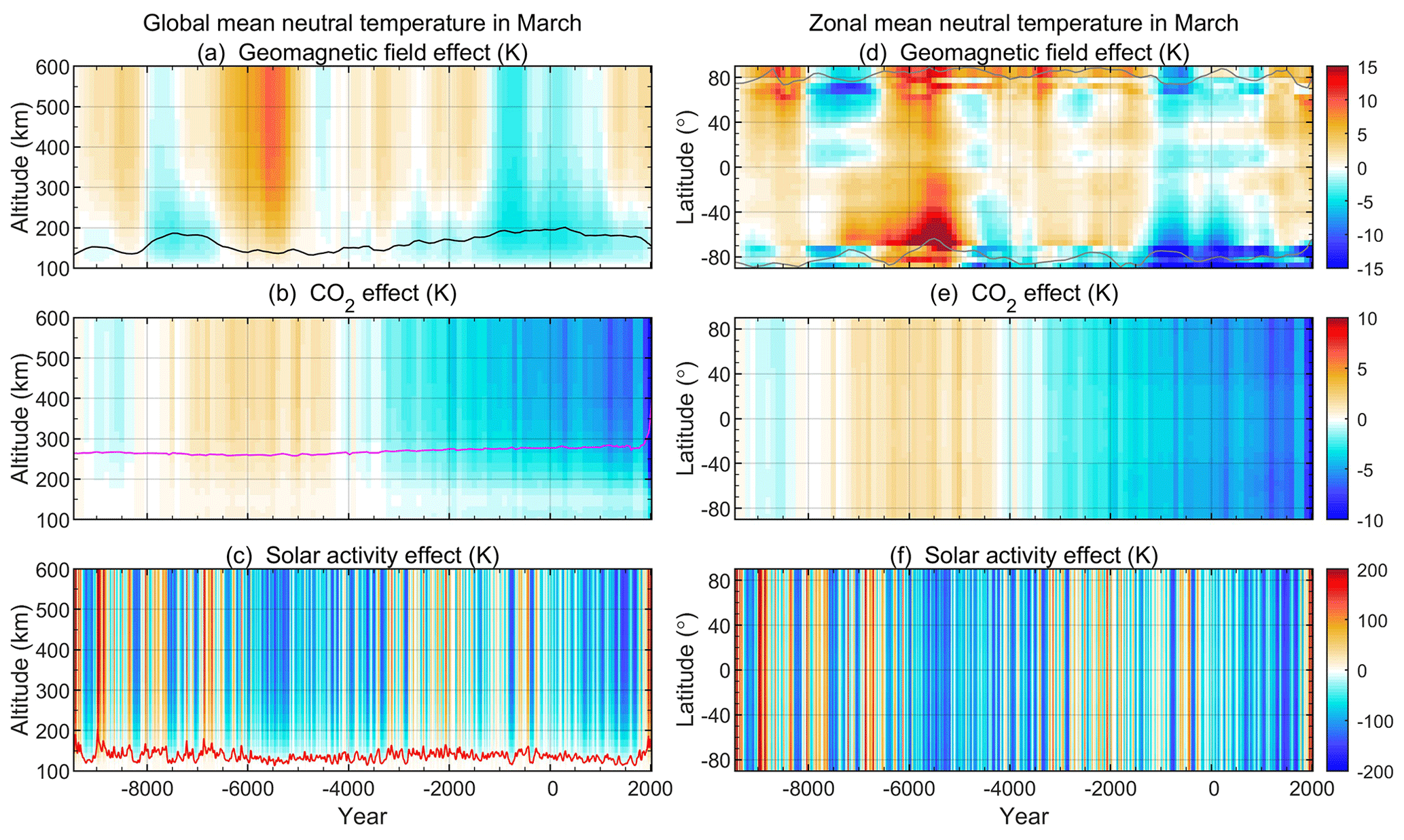
Figure 4 shows a similar pattern to Fig. 3, except that the neutral temperature variations are shown. Overall, the effects of CO₂ and solar activity on temperature are essentially the same as those on neutral density, and only the temperature change is more significant. The dramatic increase in CO₂ level in the past century has led to a decrease in global mean neutral temperature of more than 20 K, which is well in line with previous understanding (Roble and Dickinson, 1989; Cnossen, 2014). In addition, the global mean neutral temperature increases within 5 K due to CO₂ reduction between 8000 and 4000 BC. Solar activity remains the dominant factor in the neutral temperature variability, which leads to neutral temperature changes in the range of ±200 K with its own oscillations. Furthermore, the effect of the geomagnetic field on neutral temperature differs significantly from the effect on neutral density but can still be explained by the geomagnetic field structure, dipole moment strength, and Joule heating. The zonal mean temperature changes contributed by the geomagnetic field show a clear latitude variation. The neutral temperature increases by ∼ 24 K at southern latitude ∼ 65^∘ around 5500 BC, caused by a reduction in the dipole moment resulting in stronger Joule heating around the south magnetic pole. Conversely, between 1500 BC and 1000 AD, the neutral temperature in the polar regions dropped by up to 22 K due to the weakening of Joule heating caused by the increase in the dipole moment. In addition, the effect of the geomagnetic field is significantly weaker at northern latitude ∼ 10^∘, perhaps owing to tides in the lower atmosphere. Although the neutral temperature changes in the polar regions are large, the change in global mean neutral temperature due to the geomagnetic field is essentially within ±10 K at all altitudes during the Holocene. The June simulations have also been carefully analyzed (not shown here), and the effects of CO₂ and solar activity are similar to those of March, and the geomagnetic field effects differ greatly from those of March, which lead to a weakening of both the neutral density and temperature, except for an increase near 5500 BC. The contributions of geomagnetic field structure, dipole moment, and Joule heating are still evident in the June results.

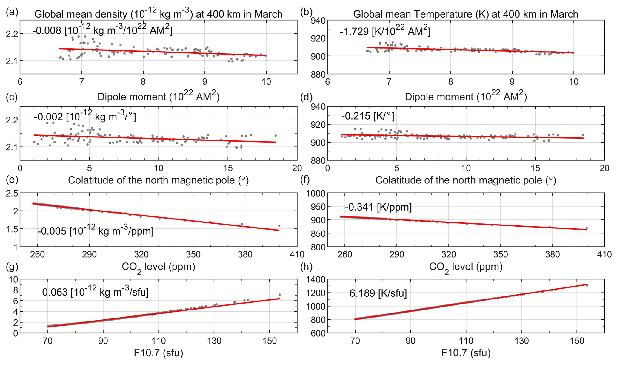
Figure 6 Simulated global mean neutral density (a, c, e, g) and temperature (b, d, f, h) at 400 km versus the geomagnetic field dipole moment (a and b, CR1), the colatitude of the north magnetic pole (c and d, CR1), the CO₂ level (e and f, CR2), and the F10.7 index (g and h, CR4–CR3) in the March equinox. The red line shows the corresponding linear fitting results, and the number in each panel is the corresponding fitted linear growth rate.

Qian et al. (2021) used the Whole Atmosphere Community Climate Model-eXtended (WACCM-X) to investigate climate change in the upper atmosphere due to changes in greenhouse gas (GHG) concentrations and Earth's magnetic field from the 1960s to the 2010s. Figures 3 and 4 show results in general agreement with those over the last century. For instance, the magnitude of the global mean neutral temperature trend caused by the change in the GHG concentrations increased with altitude and is ∼ −3 K per decade at 400 km, and the trends in both global mean neutral density and temperature due to magnetic field changes are negligible. One difference is that the trend of global mean neutral density in our results ($\sim -$2 % per decade at 400 km) is half that of Qian et al. (2021), probably because we consider a much longer timescale than Qian et al. (2021) and because we use the high-latitude convection model of Weimer (1996) rather than Heelis et al. (1982). In addition, in Figs. 3 and 4, the changes in zonal mean neutral density and temperature in the Northern Hemisphere and Southern Hemisphere over the past 2000 years are asymmetric and may be caused by the non-dipole component of the geomagnetic field. The increase in temperature and density in the Northern Hemisphere and the decrease in the Southern Hemisphere may be related to the drift of the magnetic pole position, the change in the neutral wind field, the change in the dipole moment, and the change in the particle precipitation when the auroral oval is shrinking or expanding (Zossi et al., 2020).

Figure 5 shows the effect of the three drivers on the global mean neutral density and temperature at 400 km, characterized by the deviation obtained by subtracting the simulation results of the starting year. The gray dots represent the results for each UT. Three main features can be extracted from Fig. 5. (1) The oscillation range of neutral density at 400 km due to the geomagnetic field, CO₂, and solar activity variations is [−5, 10], [−60, 5], and [−200, 400] × 10⁻¹⁴ kg m⁻³, respectively, while it is [−10, 10], [−40, 5], and [−200, 200] K for the neutral temperature. It is clear that the effect of solar activity variations is dozens of times greater than that of CO₂ and geomagnetic field variations. (2) Both the neutral density and temperature decrease with increasing CO₂. (3) The effects of CO₂ and solar activity have no universal time variation, while the effects of the geomagnetic field have significant universal time variation modulated by the dipole moment.

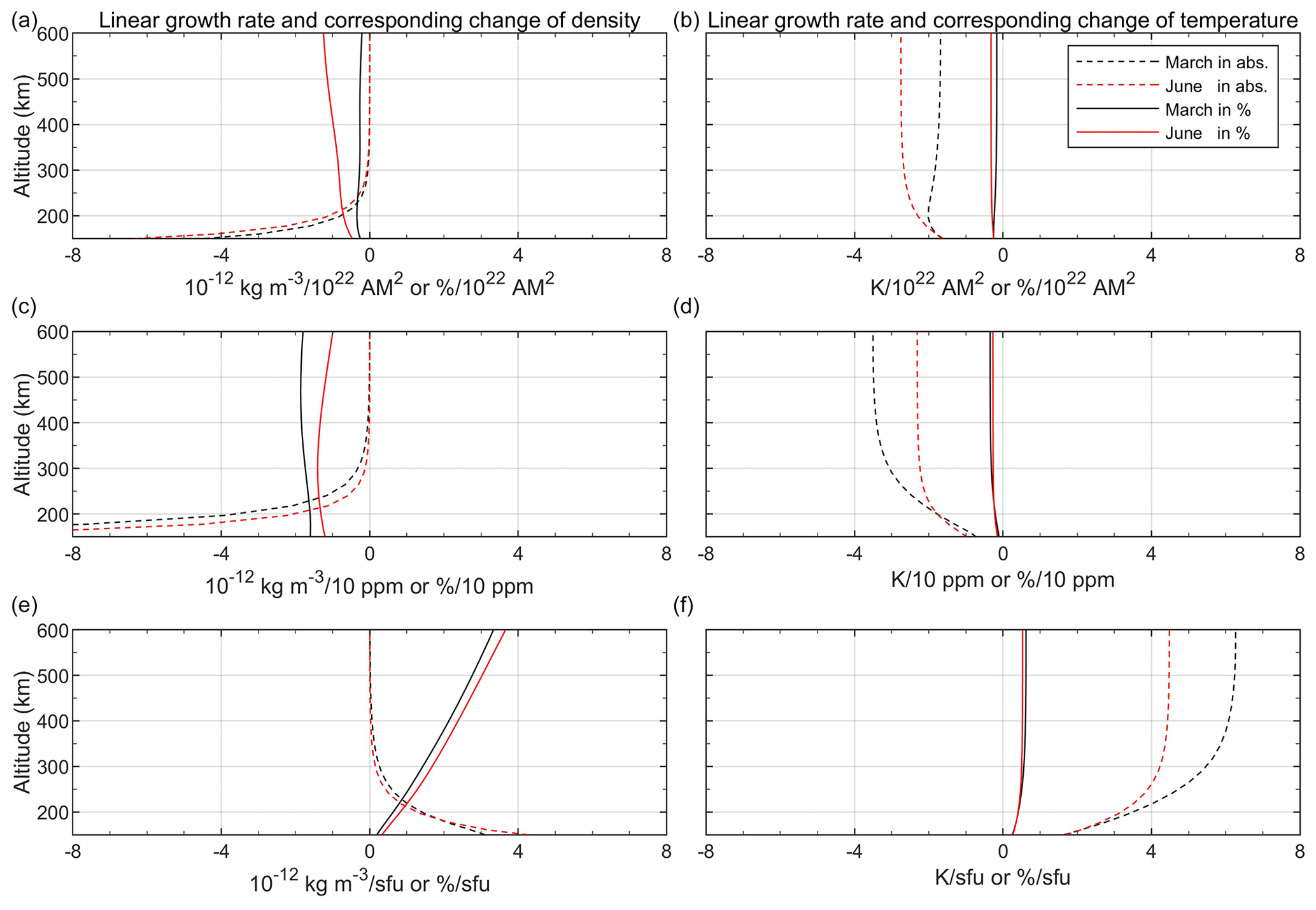
Figure 7 The altitude variations of the linear growth rate (dashed lines) and the corresponding change in percentage (solid lines) of global mean neutral density (a, b) and temperature (b, d, f) resulting from the dipole moment (a and b, CR1), the CO₂ level (c and d, CR2), and the F10.7 index (e and f, CR4–CR3) in the March equinox (black lines) and June solstice (red lines).

3.3 The long-term trends generated by the variations of the geomagnetic field, CO₂, and solar activity

From Figs. 3 to 5, it can be found that the effects of the three factors vary approximately linearly. Therefore, we calculated linear growth rates for the effects of the three factors on neutral density and temperature, as shown in the text of each panel in Fig. 6, which reveals the long-term trends of the thermosphere generated by the variations of the geomagnetic field (dipole moment and the colatitude of the north magnetic pole), CO₂, and solar activity, respectively. The gray dots in Fig. 6 are the global mean value of neutral density (left column) and temperature (right column) at 400 km in the March equinox of the corresponding year in the simulations driven by the three drivers. The red lines are the result of the least-squares fitting. The neutral density and temperature show a significant linear variation with the three drivers, while the nonlinear effect of the geomagnetic field can be found in the first and second rows, shown by the scattered gray dots on both sides of the red line. Although the fitted density is generally smaller when F10.7 is greater than 110 in Fig. 6g, the linear variation of the simulated neutral density with F10.7 is still clearly visible, only presenting a larger linear growth rate. The average value of the global mean neutral density at 400 km over the entire simulation time interval is about $\mathrm{2.26}\times {\mathrm{10}}^{-\mathrm{12}}$ kg m⁻³. Based on this value and the linear growth rate shown in Fig. 6, the effects due to changes in the geomagnetic dipole moment, the colatitude of the north magnetic pole, CO₂, and solar activity during the entire Holocene can be calculated to be about −1.4 %, −1.6 %, −31 %, and +250 %, respectively, while the effects are about −7, −4, −48, and +557 K for the neutral temperature, respectively. Solomon et al. (2019) pointed out that the temperature change from solar minimum to maximum increases by about 500 K at 400 km based on the simulation of WACCM-X, which is generally consistent with our results. Since the effect of magnetic pole position is not as large as that of dipole moment, only the dipole moment is used later to quantify the effect of the magnetic field.

Figure 7 shows the altitude variations of the linear growth rate (dashed lines) and the corresponding change in percentage (solid lines) of the global mean neutral density (left column) and temperature (right column) resulting from the three drivers in the March equinox (black lines) and June solstice (red lines). The effect of the three drivers on the neutral temperatures of March and June essentially increases with altitude, but it is close to constant above 300 km. The effect of the geomagnetic field on the neutral temperature is slightly larger in June than in March. For every 10²² Am² increase in dipole moment, the neutral temperature in June decreases by ∼ 2.7 K compared to ∼ 1.7 K in March. In contrast, CO₂ and solar activity have the opposite effect on neutral temperature, with a larger effect in March. For every 10 ppm increase in CO₂, the global mean neutral temperature above 200 km decreases by ∼ 3.5 K in March and ∼ 2.3 K in June. Akmaev and Fomichev (1998) suggested a trend of about −3.1 K per 10 ppm at 200 km in the thermosphere in April due to increasing CO₂, while Cnossen (2014) and Solomon et al. (2018) reported trends of about −1 and −1.8 K per 10 ppm above 200 km, respectively. Therefore, it is reasonable that our results are 0.8–3.5 K per 10 ppm between 150 and 600 km. For each 1 sfu increase in F10.7, the neutral temperature increase is ∼ 6.2 and ∼ 4.4 K in March and June, respectively. The effect of the three factors on neutral density is similar to that on neutral temperature. Since neutral density decreases exponentially with altitude, the effect of the three factors on neutral density (absolute value change) also decreases with altitude above 150 km, as shown in the left column of Fig. 7. To present more clearly the effect of the three factors on neutral density, the solid lines display the corresponding percentage changes using 2005 simulations of CR4 as a reference. This reveals that the effects of solar activity and dipole moment on neutral density increase significantly with increasing altitude in March and June, with a stronger effect in June, while the effect of CO₂ is basically unchanged with altitude in both March and June, with a stronger effect in March. In addition, the increasing dipole moment and CO₂ decrease the neutral density, while the rising solar activity increases the neutral density.

As mentioned in Sect. 3.2, only the effect of the geomagnetic field on the thermosphere displays the latitude and UT variations. Figure 8 shows the linear growth rate of neutral density (top row) and temperature (bottom row) at 400 km attributed to the geomagnetic field versus latitude and UT (left column) or longitude (right column). In general, an increase in the dipole moment attenuates the thermospheric neutral density and temperature at all latitudes, longitudes, and UTs. The linear growth rate is greater at high latitudes at 00:00–08:00 and 18:00–24:00 UT and can reach −3.6 ± 10⁻¹⁴ kg m⁻³/10²² Am² or −9.5 K/10²² Am², while it is about −1 ± 10⁻¹⁴ kg m⁻³/10²² Am² or −2 K/10²² Am² at other latitudes and UTs. In addition, a larger linear growth rate of up to −4.4 ± 10⁻¹⁴ kg m⁻³/10²² Am² or −8.7 K/10²² Am² is seen at all longitudes above ±60^∘ latitude, and it is also about −1 ± 10⁻¹⁴ kg m⁻³/10²² Am² or −2 K/10²² Am² in other regions. Overall, the thermosphere in the polar regions of the Southern Hemisphere is more influenced by the geomagnetic field than that in the Northern Hemisphere, while the influence of the magnetic field is weaker and of about a similar magnitude at the middle and low latitudes.

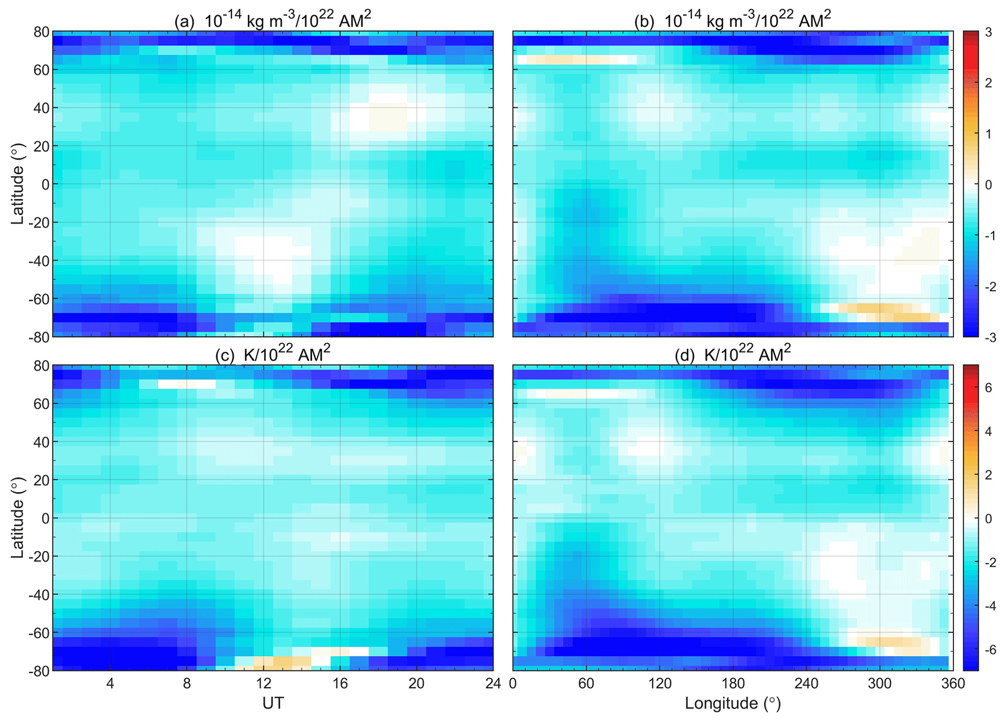
Figure 8 The latitude and longitude variations of the linear growth rate of UT mean neutral density (b) and temperature (d) due to the geomagnetic field. Panels (a) and (c) are the corresponding linear growth rate of zonal mean neutral density and temperature versus latitude and UT.

3.4 Future projections

As the number of human space missions increases explosively, more and more spacecraft will operate in the thermosphere, so projecting the future state of the thermosphere is also important to human life. Based on the IPCC projections of greenhouse gas emissions under different scenarios (IPCC, 2014), we can simply and reasonably assume that CO₂ concentrations will rise by 400 ppm over the next century. Therefore, according to the calculations shown in Table 2, the global mean neutral density will decrease by ∼ 70 % and ∼ 50 % in March and June, respectively, due to a 400 ppm increase in CO₂. This is generally consistent with the trend of about −6.1 % ± 0.8 % per decade throughout the 21st century projected by Cnossen (2022). Also, from Fig. 7, it can be concluded that the neutral temperatures in March and June will decrease by ∼ 114 and ∼ 84 K, respectively. This is larger than the projections (∼ 60 K) of Cnossen (2022).

The dipole moment decreases by about 3.5 % over the next 50 years based on the prediction by Aubert (2015), causing an increase in global mean neutral density of up to 1 % above 500 km according to the simulations of Cnossen and Maute (2020). However, the increase in the global mean neutral density is projected to be ∼ 0.08 % and ∼ 0.25 % in March and June, respectively, based on our calculated linear growth rate. In addition, we can also project that the temperature increase due to the decrease in the dipole moment in March and June is about 0.5 and 0.7 K, respectively. As shown in Fig. 8, the effect of the geomagnetic field is strongly dependent on UT and geographic location, so the global mean state projection is provided for reference only. Furthermore, the effect of geomagnetic field variation is negligible compared to the effect of rising CO₂ over the next 100 years. Based on WACCM-X simulations for the period 1960–2010, Qian et al. (2021) suggested that, although the magnetic field driver is important in the longitude sector ∼120^∘ W–20^∘ E, it drove both negative and positive trends in roughly equal amounts, and consequently its contributions to the global average trends in the thermosphere are negligible on shorter timescales.

4 Conclusions

In this study, the evolution of the thermosphere during the Holocene (from 9455 BC to 2015 AD) was simulated using the independently developed global ionosphere–thermosphere theoretical model GCITEM-IGGCAS, driven by the realistic geomagnetic field model, CO₂ level, and solar activity derived from modern measurements and ancient natural media. Furthermore, through a series of control simulations, we quantify the thermospheric temperature and density changes due to variations in the geomagnetic field, CO₂ levels, and solar activity. The main conclusions are presented below.

The climatological morphology of the global thermosphere during the Holocene is reconstructed for the first time. Thermospheric neutral density is mainly controlled by solar activity and modulated by CO₂ and the geomagnetic field. Typically, the geomagnetic field configuration directly affects the morphology of the equatorial mass anomaly structure of the thermosphere, while CO₂ mainly affects the magnitude of the neutral density and temperature. In general, the frequent oscillations of solar activity contribute more than 80 % of the thermospheric variability, while the contributions of CO₂ and the geomagnetic field are both less than 10 %. The effect of CO₂ is comparable to that of the geomagnetic field throughout the Holocene for the global mean neutral density and temperature but becomes more significant after 1800 AD. Only the effect of the geomagnetic field is strongly dependent on the universal time and geographical location, and the weakening of the dipole moment leading to an increase in Joule heating in the polar region thus makes the thermosphere change more intense than the effect of CO₂. Overall, the higher the altitude, the larger the effect of the three drivers on the neutral density and temperature.

Both the thermospheric neutral density and temperature vary approximately linearly with the dipole moment of the geomagnetic field, CO₂, and F10.7 index of solar activity. The global mean variability of the neutral density at 400 km during the March equinox due to changes in the geomagnetic dipole moment, CO₂, and solar activity during the entire Holocene can be about −1.4 %, −31 %, and +250 %, respectively, while the effects are about −7, −48, and +557 K for the neutral temperature, respectively. In addition, there is a clear altitude and seasonal variation in the thermosphere change due to an increase in the unit of the dipole moment, CO₂, and solar activity. Different factors produce different seasonal variations in thermosphere changes. The increasing dipole moment and CO₂ decrease the neutral density and temperature, while the rising solar activity increases them.

We project that a 400 ppm increase in CO₂ will result in a 50 %–70 % reduction in global mean thermospheric neutral density depending on the season, while neutral temperatures will decrease by 84–114 K. This is enough to change the orbit and lifetime of spacecraft and space debris, which deserves the attention of future space missions. The effect of decreasing dipole moments of the geomagnetic field over the next 100 years on the global mean thermospheric neutral density and temperature is negligible, but the effect of changing magnetic field configurations (e.g., magnetic pole positions) on the thermosphere should be considered, especially in the polar regions.