the Creative Commons Attribution 4.0 License.
the Creative Commons Attribution 4.0 License.
 | 01 Jun 2023
Comment on “Climate consequences of hydrogen emissions” by Ocko and Hamburg (2022)
Ken Caldeira
In this commentary, we provide additional context for Ocko and Hamburg (2022) related to the climate consequences of replacing fossil fuels with clean hydrogen alternatives. We first provide a tutorial for the derivations of underlying differential equations that describe the radiative forcing of hydrogen emissions, which differ slightly from equations relied on by previous studies. Ocko and Hamburg (2022) defined a metric based on time-integrated radiative forcing from continuous emissions. To complement their analysis, we further present results for temperature and radiative forcing over the next centuries for unit pulse and continuous emissions scenarios. Our results are qualitatively consistent with previous studies, including Ocko and Hamburg (2022). Our results clearly show that for the same quantity of emissions, hydrogen shows a consistently smaller climate impact than methane. As with other short-lived species, the radiative forcing from a continuous emission of hydrogen is proportional to emission rates, whereas the radiative forcing from a continuous emission of carbon dioxide is closely related to cumulative emissions. After a cessation of hydrogen emissions, the Earth cools rapidly, whereas after a cessation of carbon dioxide emissions, the Earth continues to warm somewhat and remains warm for many centuries. Regardless, our results support the conclusion of Ocko and Hamburg (2022) that, if methane were a feedstock for hydrogen production, any possible near-term consequences will depend primarily on methane leakage and secondarily on hydrogen leakage.
- Article
(1441 KB) - Full-text XML
-
Supplement
(1741 KB) - BibTeX
- EndNote


In a recent paper, Ocko and Hamburg (2022) examined the climate consequences of replacing fossil fuel technologies with clean hydrogen alternatives. The paper accounted for a range of hydrogen and methane emission rates for two types of clean hydrogen production pathways, i.e., green hydrogen produced via renewables and water, and blue hydrogen produced via steam methane reforming with carbon capture, usage, and storage (CCUS). They calculated the time-integrated radiative forcing using equations derived recently for hydrogen based on chemistry–climate modeling experiments (Warwick et al., 2022). Ocko and Hamburg (2022) found that high emission rates of hydrogen could diminish net climate benefits of clean hydrogen technologies, and high emission rates of methane might lead to net climate disbenefits for blue hydrogen in the near term (e.g., 20-year timescale).
Here, we provide context for understanding the results of Ocko and Hamburg (2022) in three different ways: (1) we present equations underlying the time evolution of hydrogen and its radiative and thermal consequences and solve them analytically for unit pulse and continuous hydrogen emissions scenarios; (2) we present global mean temperature and radiative forcing in the time domain covering 500 years; and (3) we examine three scenarios, including a unit pulse, a limited duration (square wave), and a continuous emissions framework. Our aim here is to complement Ocko and Hamburg (2022), which emphasizes the near term, with an analysis that places greater emphasis on long-term outcomes using newly developed equations.
We derive and apply equations underlying the estimate of radiative forcing from hydrogen (H2) emissions as presented by Warwick et al. (2022), relying heavily on parameter values from Ocko and Hamburg (2022) (Table S1 in the Supplement). Equations describing the radiative forcing of carbon dioxide (CO2) and methane (CH4) are based on Myhre et al. (2013). We estimate the global mean temperature change from emissions of CO2, CH4, or H2 using a linearized Green's function approach and apply these equations to simple idealized cases. The calculation of the global mean temperature response is based on Gasser et al. (2017).
2.1 Indirect forcing from hydrogen
The system that describes the radiative forcing from H2 emissions modeled by Warwick et al. (2022) and later used in Ocko and Hamburg (2022) is a representation of the following differential equations.
The change of H2 molar mass relative to an unperturbed background condition, as a function of the time horizon t in units of year, is represented by a source function and a decay term , where is the molar mass of H2 and is the perturbation lifetime of H2:
The presence of additional H2 in the atmosphere changes the decay of atmospheric CH4 and also results in the production of ozone (O3) and stratospheric water vapor (H2O). Underlying equations for perturbations to atmospheric molar masses of CH4, O3, and stratospheric H2O induced from additional atmospheric H2 (denoted by superscripts) are
Here, , , and are the respective molar masses of CH4, O3, and H2O resulting from additional atmospheric H2; , , and are factors representing the impact of remaining H2 in the atmosphere on the atmospheric molar mass of these respective species; and , , and are perturbation lifetimes of these respective species.
For the special case of a unit pulse perturbation of H2 into an unperturbed background condition at time zero, these equations can be solved analytically. The respective solutions to Eqs. (1) and (2) under conditions , , , , and are
and
The corresponding radiative forcing is the product of the resulted molar mass and scaling factors , , and that convert molar mass to watts per meter squared (W m−2). The chemically adjusted radiative forcing, , for CH4 uses factors f1 and f2 (Myhre et al., 2013) to represent the effect on O3 and stratospheric H2O:
The indirect radiative forcing from a unit pulse emission of H2, , is thus the sum of radiative forcing from all three radiatively active perturbations:
Inserting Eq. (4), we have
For a 1 kg unit pulse emission case, the time-integrated radiative forcing to a specified time horizon, H, is defined to be the absolute global warming potential (AGWP) (Myhre et al., 2013). Thus, AGWP can be represented as
which can be rewritten as
Equation (7) is the response to a unit pulse emission of H2 taking into consideration radiative forcing adjustments to CH4 as in Ocko and Hamburg (2022). Because we are considering a linear system, we can use this impulse response function to derive the radiative forcing from an arbitrary H2 emission function :
Considering a continuous unit emission scenario where
this leads to radiative forcing under a continuous emission scenario:
In a linear system, the time-integrated radiative forcing from a unit pulse emission to some time horizon t0 is mathematically equivalent to the radiative forcing at time t0 from continuous unit emissions:
Ocko and Hamburg (2022) used a metric that is equal to the time-integrated radiative forcing of continuous emissions to time horizon H. Since the AGWP has been defined as the time-integrated radiative forcing from the instantaneous release of 1 kg of a trace substance (Myhre et al., 2013), here we define the time-integrated radiative forcing under a continuous emission scenario as continuous absolute global warming potential (CAGWP):
Comparing Eq. (12) with Eq. (7a), we can see that the CAGWP metric is equivalent to the AGWP metric, except that the radiative forcing at time 0 is weighted by H, and the radiative forcing at time H is weighted at 0, with a linear ramping of weights in between by the number of years to the end of the time horizon. Equation (12) illustrates that time-integrated metrics under continuous emissions put heavy weights on the short-term effect.
Expanding Eq. (12), we have
Equations (10) and (13) consider continuous emissions through the whole period. Equations considering a continuous emission to time tp are shown in Sect. S1 in the Supplement. Reproductions of the three components in Warwick et al. (2022) and Ocko and Hamburg (2022) are shown in Sect. S2. When used to estimate radiative forcing for identical cases, numerical differences between our equations and equations presented by Warwick et al. (2022) are small and are unlikely to make a material difference.
2.2 Forcing from CO2 and CH4
Here, we show radiative forcing and time-integrated radiative forcing functions for CO2 and CH4. Parameters are defined and values are given in Table S1. Radiative forcing for a unit pulse emission of CO2 and CH4 is represented as (Myhre et al., 2013)
The AGWP for a unit pulse emission is
Radiative forcing for continuous emissions of CO2 and CH4 can be represented as
And the corresponding CAGWP is
2.3 The global mean temperature response
For a linear system, the absolute global temperature change potential (AGTP), defined as the change of global mean surface temperature realized at a given time horizon from a pulse or continuous emissions of any gas i, can be represented as a convolution function (Myhre et al., 2013; Gasser et al., 2017):
In Eq. (22), Ri(t) is the radiative forcing for unit pulse or continuous emissions of gas i and T(t) indicates the temperature response to a unit forcing that can be represented as a sum of exponentials:
where λ is a constant that corresponds to the equilibrium climate sensitivity, , and dj is the response time. Two exponential terms (M=2) are normally used in previous studies, with the first term associated with the response of the ocean mixed layer and the higher order associated with the response of the deep ocean (Gasser et al., 2017). In our central cases, we focus on using the equation from Geoffroy et al. (2013):
Uncertainty in the temperature response function is shown in Sect. S3.
2.4 Simulations and assumptions
As in Ocko and Hamburg (2022), we focus on comparing the climate impact of replacing fossil fuel technologies with clean hydrogen alternatives. Climate impacts from hydrogen or fossil fuels are the summation of climate impacts of one or more components in a linear system (Sect. S4).
In this commentary, we analyze the climate impact per 1 kg consumption of green and blue H2 and corresponding impacts from the avoided CO2 emissions. We consider consistent assumptions as in Ocko and Hamburg (2022). For example, the kilogram amount of CH4 required to produce blue H2 is 3 times the kilogram amount of H2 used, 1 kg consumption of H2 would avoid 11 kg of CO2 emissions (additional cases, i.e., 5 or 15 kg of avoided CO2 emissions, are examined as well), and burning 1 kg of CH4 would emit 2.75 kg of CO2. Also, we take the same consistent leakage rate assumptions for CH4 and H2 to generate two central cases: a low-leakage case with 1 % H2 and 1 % CH4 leakage rates, and a high-leakage case with 10 % H2 and 3 % CH4 leakage rates (see detailed discussion underlying these assumptions in their paper).
We focus our discussions on three H2 consumption scenarios: a 1 kg pulse consumption, 0.01 kg yr−1 continuous consumption lasting for 100 years, and 0.01 kg yr−1 continuous consumption lasting for 500 years. Results for 20-, 100-, and 500-year horizons are summarized in Tables S2 to S5.
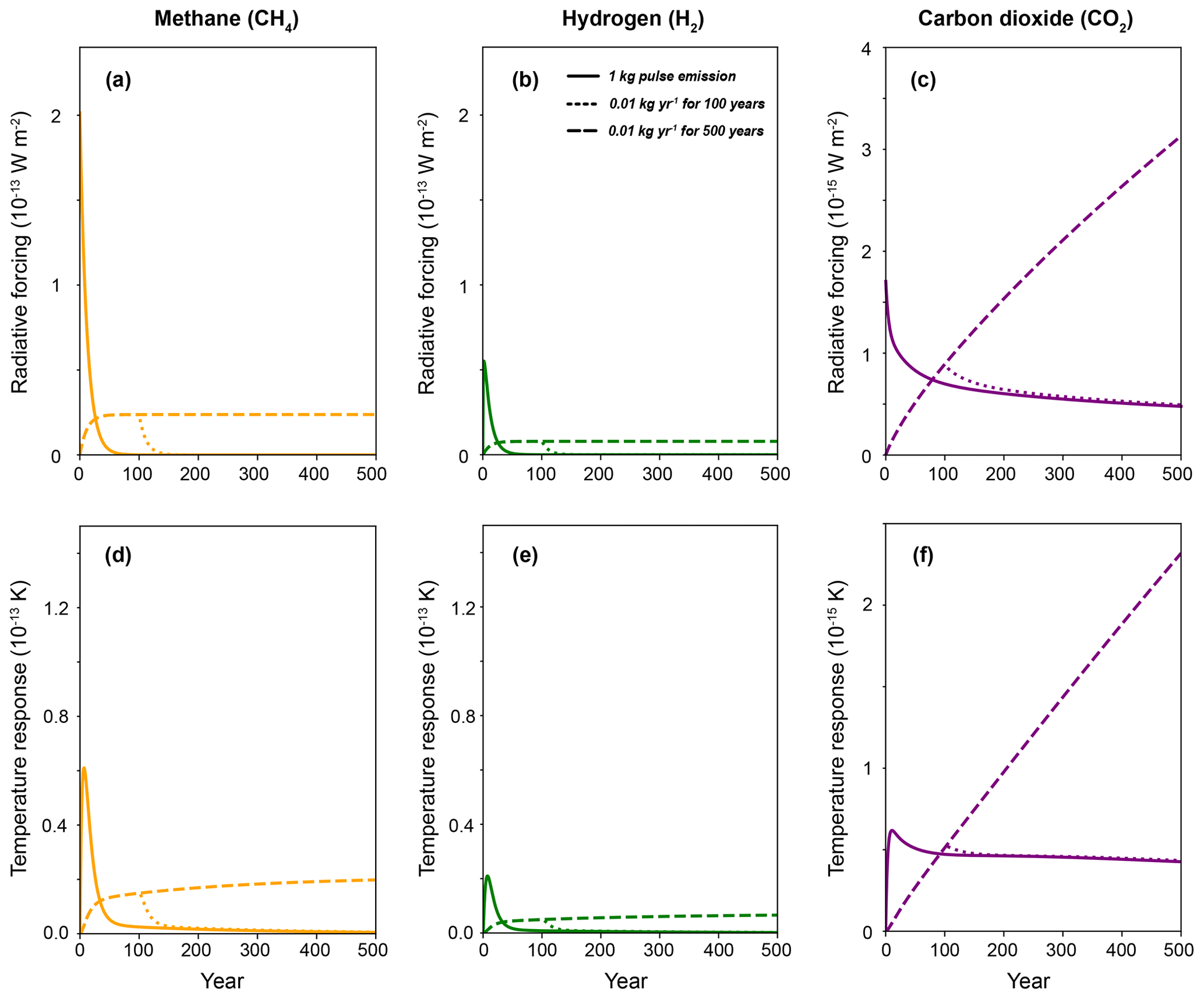
Figure 1Climate impact from emissions of respective species. Radiative forcing (a–c) and global mean temperature response (d–f) caused by emissions of methane (CH4), hydrogen (H2), and carbon dioxide (CO2). Three emission scenarios are considered: a 1 kg pulse emission, 0.01 kg yr−1 continuous emissions lasting for 100 years, and 0.01 kg yr−1 continuous emissions lasting for 500 years. CH4 and H2 share the same y axis, the maximum value of which is 60 times relative to that of CO2. Radiative forcing from continuous emissions of H2 and CH4 is proportional to the emission rate and decays rapidly once ceased, whereas radiative forcing from CO2 is closely related to the cumulative amount and will last for longer timescales. Figures showing only 100-year results are plotted in Fig. S12.
3.1 Climate impact of individual gas
We first examine the time-evolving climate impact from emissions of carbon dioxide (CO2), methane (CH4), and hydrogen (H2), respectively. Similarly, we consider three emission scenarios: a 1 kg pulse emission, 0.01 kg yr−1 continuous emissions lasting for 100 years, and 0.01 kg yr−1 continuous emissions lasting for 500 years.
Figure 1 shows the climate impact of individual species under various emission scenarios. Results showing ratios of CH4 and H2 to CO2 are plotted in Fig. S1 in the Supplement. For the 1 kg pulse emission scenario, all species produce the largest climate impacts within the first few years and decay over time. Soon after emission, per kilogram emitted, CH4 and H2 show much larger impacts compared to CO2. The global warming potential is typically defined for a 1 kg pulse emission of gas (Myhre et al., 2013), which will lead to different immediate changes in their atmospheric concentration when viewed on a molar basis. Figure S2 shows that when considering a 1 ppb increase of these gases, CH4 still generates a much larger warming potential, whereas H2 and CO2 show the same order of magnitude impacts on radiative forcing and temperature in the first decade.
The climate impact of CH4 and H2 decays substantially faster than CO2 along with their concentrations (perturbation lifetime used is 11.8 years for CH4 and 1.9 years for H2). For example, the radiative forcing of CH4 and H2 for the 1 kg pulse emission scenario is smaller than that of CO2 after ∼ 65 and 50 years and approaches zero after 100 years. We do not consider conversions of the decayed CH4 to CO2, which will add more long-term impacts for CH4 emissions (Forster et al., 2021) as shown in Fig. S3. This conversion should not be considered in the case of CH4 perturbations brought about by H2 emissions, because there is no net addition of carbon to the atmosphere in this case. In contrast, the radiative forcing of CO2 is still 28 % of its maximum value at the 500-year time horizon. Temperature response behaves similarly to radiative forcing but at a slower rate due to the inertia of the climate system. Impacts of considering different H2 perturbation lifetimes (i.e., 1.4 and 2.5 years) are shown in Fig. S4.
For 0.01 kg yr−1 continuous emission cases, there is an accumulation of CO2 concentration in the atmosphere, leading to monotonic increases in radiative forcing and temperature. If emissions stop abruptly after 100 years, the climate impacts of CO2 slowly converge with those under the 1 kg emission case and stay roughly stable, because the effects of atmospheric concentration decrease are approximately offset by the effects of ocean warming. Due to the shorter perturbation lifetime of CH4 and H2, their atmospheric concentrations reach equilibrium under continuous emission scenarios with magnitudes depending on the emission rates, and radiative forcing reaches a stable level after a few decades. Global mean temperature continues to increase slowly due to the thermal inertia of the climate system. If emissions stop abruptly after 100 years, their concentrations would decrease rapidly and reach zero within decades. The longer perturbation lifetime of CO2 results in more prominent longer-term climate impacts under both pulse and continuous emission scenarios.
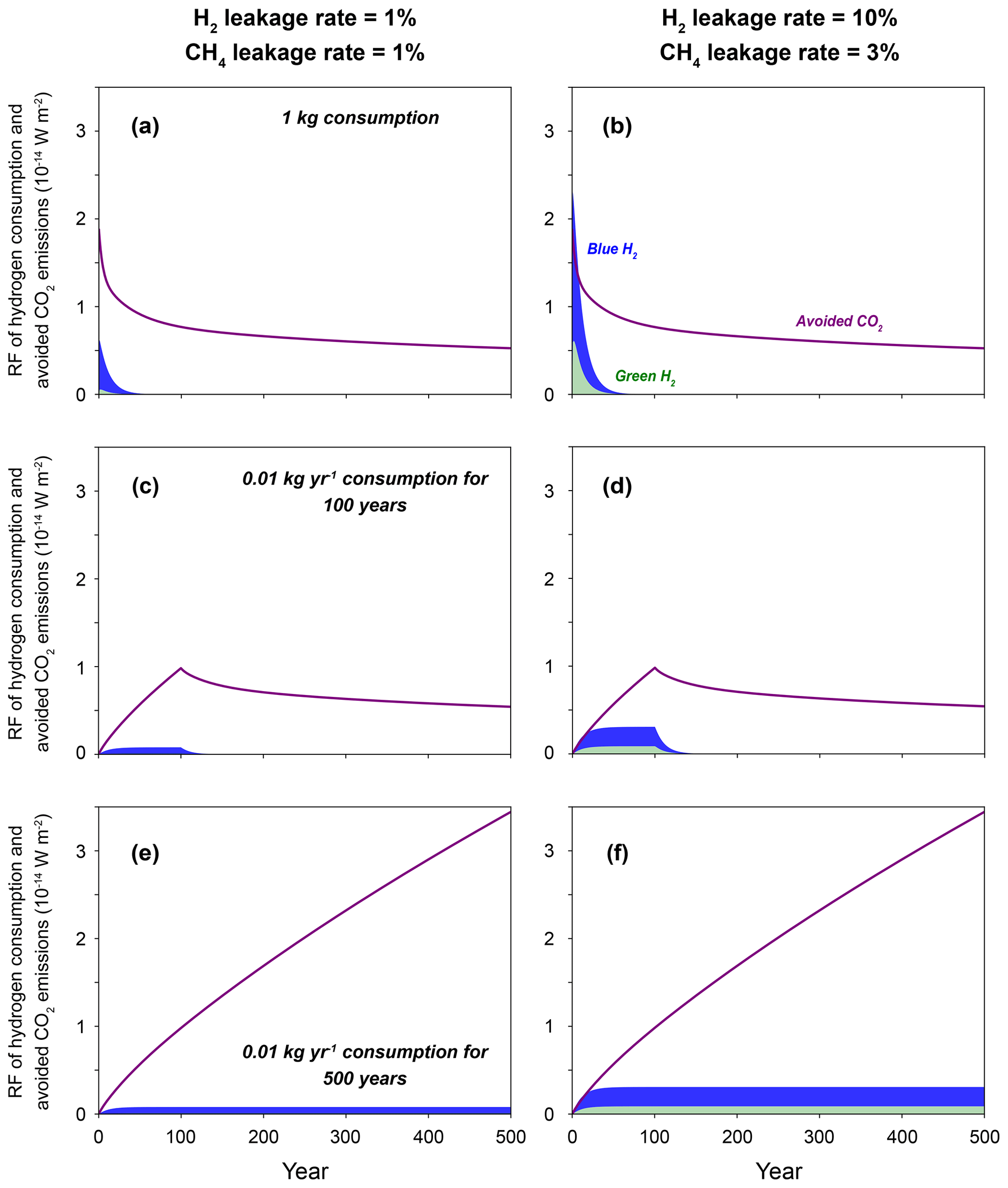
Figure 2Radiative forcing from consumption of green hydrogen (H2), blue H2, and avoided CO2 emissions. Three cases are considered: (a, b) a 1 kg consumption of H2, (c, d) 0.01 kg yr−1 continuous consumption of H2 lasting for 100 years, and (e, f) 0.01 kg yr−1 continuous consumption of H2 lasting for 500 years. Panels (a), (c), and (e) show cases with 1 % H2 and 1 % CH4 leakage rates, and panels (b), (d), and (f) show cases with 10 % H2 and 3 % CH4 leakage rates. CH4 leakage contributes primarily to the warming potential of blue H2 consumption, while H2 leakage plays a secondary role. For the longer term, radiative forcing from carbon dioxide is substantially larger than that from clean H2 alternatives. Figures showing only 100-year results are plotted in Fig. S13.

Figure 3Same as Fig. 2 but for the global mean temperature response. Figures showing only 100-year results are plotted in Fig. S14.
3.2 Climate impact of hydrogen and fossil fuels
Under the low-leakage scenario (i.e., 1 % H2 and 1 % CH4 leakage rate), both green and blue H2 produce smaller radiative forcing and global mean temperature increases compared to the avoided CO2 emissions (Figs. 2 and 3), indicating net climate benefits of replacing fossil fuels with clean hydrogen alternatives. Compared to green H2, leakages of CH4 from blue H2 add substantial additional warming within the first few decades. For the 1 kg pulse consumption scenario, the climate impact of green and blue H2 decays rapidly to zero within the first few decades (conversion of decayed CH4 to CO2 not included), whereas the climate impact of avoided CO2 emissions becomes roughly stable with time. Continuous consumption of H2 would lead to stable radiative forcing and temperature change at longer timescales with magnitudes depending on consumption levels, and such impacts will adjust quickly if future leakage rates change. Meanwhile, continuous consumption of fossil fuels leads to accumulation of CO2 concentration and increasing climate responses. Even if CO2 consumption is ceased, its impacts would last for hundreds of years.
Under the high-leakage scenario, the additional leakage of H2 (i.e., 10 % vs. 1 % H2 leakage rate) reduces the short-term climate benefits of green H2, and the additional leakage of CH4 (i.e., 3 % vs. 1 % CH4 leakage rate) further leads to net disbenefits for blue H2 in the first few years, when compared to avoided CO2 emissions (Figs. 2 and 3). In both the low- and high-leakage cases, CH4 adds more warming than H2 does (Fig. S5). Because of the shorter lifetimes of H2 and CH4, net climate benefits for blue H2 are observed after ∼ 12 and 20 years under different emission scenarios for the high-leakage case. The climate impacts of H2 become orders of magnitude smaller than that of CO2 emissions as time evolves.
In our central cases, we do not include CH4 leakages when calculating climate impacts for the avoided CO2 emissions, which are included for blue H2. Under all emission scenarios, using the same CH4 leakage rates for CH4 combustion and H2 production (Figs. S6 and S7) substantially increases the warming potentials from the avoided CO2 emissions, especially for the short-term results, leading to net climate benefits for both clean hydrogen alternatives. Consideration of conversion of the decayed CH4 to CO2 further increases the long-term climate impacts for both blue H2 and the avoided CO2 emission cases that contain CH4 leakage (Figs. S6 and S7). As in Ocko and Hamburg (2022), considering that different amounts of avoided CO2 emission for per kilogram of H2 consumption (e.g., 5 or 15 kg CO2 avoided per kilogram of H2 consumption) can affect both short-term and long-term climate impacts (Fig. S8). In contrast, considering different H2 perturbation lifetimes or climate response functions has minor effects (Figs. S6, S7, and S9). Here, we do not cover all uncertainties but give some first-level impressions of how different parameters can affect results presented in this analysis.
Finally, Ocko and Hamburg (2022) quantified the net climate benefits of consuming H2 compared to the avoided CO2 emissions by comparing the time-integrated radiative forcing from continuous emissions of both gases. This metric overpredicts the amount of warming that would be produced by CH4 and H2 leakage relative to the warming that would have been caused by the avoided CO2 emissions over time (Fig. S10). This result is similar to that of Allen et al. (2016) showing that, for pulse emissions and any time horizon longer than a decade, the global mean relative temperature response metric (i.e., GTP) would be lower than values of the time-integrated relative radiative forcing (i.e., GWP).
The radiative forcing calculation presented here is a linear approximation, with radiative forcing increasing linearly with concentration, when in fact absorption bands become increasingly saturated at higher concentrations, and this results in less sensitivity at higher concentrations. The radiative forcing calculation assumes an unchanging background atmospheric composition, whereas it is likely that the climate impact of an emission will depend on the background climate state (Duan et al., 2019; Robrecht et al., 2019). For instance, the indirect radiative forcing of hydrogen (H2) through its effect on the lifetime of methane (CH4) might depend on the background CH4 concentration. The effectiveness of radiative forcing at affecting temperature can vary substantially from gas to gas (Hansen et al., 1997; Modak et al., 2018). In addition, the framework used here only compares H2 with the avoided carbon dioxide (CO2) emissions, while fossil fuel adoptions are associated with emissions of other radiatively active species and air pollutants (IPCC, 2018).
Many important uncertainties persist. For example, we considered the chemical adjustment to radiative forcing for CH4 due to effects on ozone (O3) and stratospheric water vapor (H2O), as considered by Ocko and Hamburg (2022). There are other effects that have been included in previous works, which would affect the warming impact of CH4 emissions (Boucher et al., 2009; Shindell et al., 2009). There are uncertainties related to cloud radiative effects from thermodynamic adjustments and aerosol–cloud interactions (O'Connor et al., 2022). There are additional uncertainties related to the fast physical radiative forcing adjustments to dioxide, O3, and other radiatively active gases (Smith et al., 2018). Co-emissions from fossil fuel combustions (e.g., aerosol precursors) can also affect climate and public health (Lelieveld et al., 2019). Unlike long-lived CO2, the climate impact of short-lived forcers might depend on locations of emissions (Persad and Caldeira, 2018; Burney et al., 2022). While their radiative forcing might diminish quickly after emission ceasing, indirect impacts from these short-lived forcers (e.g., by affecting carbon sinks and atmospheric CO2 levels) could last longer, introducing additional uncertainties (Fu et al., 2020). None of these considerations are expected to be of sufficient magnitudes to qualitatively alter key conclusions presented here.
Ocko and Hamburg (2022) propose a metric, which we call CAGWP, that involves the integral of radiative forcing for continuous emissions, which differs from the standard GWP metric based on a unit emission of 1 kg of gas. While the GWP metric has been widely used to compare the climate impact of different greenhouse gases, it may not be the best predictor of climate impacts. For example, Allen et al. (2016) have argued that the GWP metric overemphasizes the long-term climate effect of short-lived gases such as CH4. The CAGWP metric proposed by Ocko and Hamburg (2022) emphasizes short-lived gases to an even greater extent than the customary GWP metric. We have shown that the CAGWP metric is equivalent to a front-loaded weighted integral of a pulse emission. The 100-year CAGWP metric weights the 1st year after an emission 99 times, whereas it weights the 99th year after an emission only once.
There are different motivations for reducing warming at various timescales. One motivation is to avoid near-term climate damage that might come, for example, from increasing storm or drought intensity. Another motivation is to avoid long-term climate damage that might come, for example, from the melting of the large ice sheets (Pattyn et al., 2018) or from making parts of the tropics effectively uninhabitable (Dunne et al., 2013; Sun et al., 2019). Decision-making can balance near-term and long-term risks and identify opportunities to address both kinds of risk simultaneously.
Different climate forcing agents differ in their degrees of reversibility. To a close approximation, on the timescale of decades or more, temperature change from CH4 or H2 emissions are proportional to rates of emission, whereas temperature change from CO2 is proportional to cumulative emission (Jones et al., 2006; Allen et al., 2009). This important distinction is not captured by the CAGWP metric proposed by Ocko and Hamburg (2022).
Considering how different market sizes would affect the overall impact of H2 is beyond the scope of this analysis. Blue H2, despite its larger climate impacts, is currently the dominant way of producing H2. Meanwhile, the additional climate benefits from green H2 have been recognized that will likely play a greater role in some regions (EUR-Lex, 2022) in the future. It is clear that electrolytic H2 made with carbon-emission-free electricity would produce less climate change than H2 made using CH4 as a feedstock; people use steam–methane reforming to produce H2 typically because it costs less than electrolysis.
Our analysis confirms the results of Ocko and Hamburg (2022) under consistent assumptions but complements their presentation with additional uncertainty analysis and a longer-term perspective. While we confirm the results presented in Ocko and Hamburg (2022), it is clear that over longer time horizons (e.g., 100 years), substituting blue or green hydrogen (H2) for fossil fuels will result in much less climate change.
We have developed a tutorial for the derivations of underlying differential equations that describe the radiative forcing of H2 emissions, which differ slightly from equations relied on by previous studies. In line with previous studies (Fuglestvedt et al., 2010; Allen et al., 2016; Balcombe et al., 2018), both the radiative forcing and global mean temperature response from H2 and methane (CH4) are proportional to the underlying emission rates, whereas climate impacts from carbon dioxide (CO2) are closely related to cumulative emissions. For the same quantity of emissions, H2 shows consistently smaller climate impact than CH4. High leakage rates of CH4 contribute primarily to the high warming potential of methane-derived H2 production, with high H2 leakage rates playing a secondary role. As shown by Ocko and Hamburg (2022), blue H2 with a CH4 leakage rate of 3 % and a H2 leakage rate of 10 % could produce more warming in the first 20 years after the release. However, even with these high-leakage rates, warming from blue H2 100 years later would be only a small portion of the warming from the fossil fuels it replaced. In contrast to the climate impact of CO2 emissions, which persist for many millennia (Archer, 2005; Solomon et al., 2009), climate impacts decay on the timescale of decades after a cessation of CH4 or H2 emissions.
Consideration of CH4 leakage associated with burning natural gas can have a substantial effect on results. Including the CH4 leakage associated with fossil fuel combustion would increase its short-term impact and might lead to net short-term climate benefit for blue H2 under greater leakage rates. Other factors, including the H2 lifetime and different climate response functions, are relatively less important.
Ocko and Hamburg (2022) propose that the climate impact of blue and green H2 be evaluated with the use of a metric that strongly weights near-term radiative forcing relative to long-term radiative forcing from individual pulse emissions.
We emphasize that to attain near-term climate benefits from “blue” H2 that dominates current markets depends critically on achieving low CH4 leakage rates. “Green” H2 produced by electrolysis using carbon-emission-free electricity has a small climate impact relative to the impact of the fossil fuels that H2 would replace, while very high H2 leakage rates could pose some climate concern and undercut accomplishing net zero emission goals. Safety and cost considerations may motivate the reduction of hydrogen leakage (Nugroho et al., 2022). In all cases considered, relative to fossil fuel combustion and associated emissions, both blue and green H2 show large long-term climate benefits even with high-leakage rates.
Scripts used to derive equations presented in this analysis are written in Wolfram Mathematica and are available online at https://doi.org/10.5281/zenodo.7346379 (Duan and Caldeira, 2022). Scripts used to calculate numbers and plot figures in this analysis are written in Python and are available online at https://doi.org/10.5281/zenodo.7346379 (Duan and Caldeira, 2022).
All parameter values used to evaluate the climate impact of different species in this paper have been taken directly from previous studies, which are listed and cited in the paper (e.g., Ocko and Hamburg, 2022; Myhre et al., 2013; Gasser et al., 2017).
The supplement related to this article is available online at: https://doi.org/10.5194/acp-23-6011-2023-supplement.
LD and KC designed the simulations, developed the equations, and did the calculations. LD prepared the initial paper and both of them reviewed and edited the paper.
In the interest of transparency, we would like to point out that Ken Caldeira is an employee of a non-profit organization that funds early commercial demonstration projects related to clean alternatives that can displace carbon-intensive technologies, and this can include clean hydrogen to decarbonize industry. In the further interest of transparency, note that Lei Duan is a consultant for a for-profit entity that has no known investments related to clean hydrogen.
Publisher's note: Copernicus Publications remains neutral with regard to jurisdictional claims in published maps and institutional affiliations.
This work is supported by a gift from Gates Ventures LLC to the Carnegie Institution for Science. The authors thank Leslie Willoughby for language polishing.
This paper was edited by Andreas Engel and reviewed by two anonymous referees.
Allen, M. R., Frame, D. J., Huntingford, C., Jones, C. D., Lowe, J. A., Meinshausen, M., and Meinshausen, N.: Warming caused by cumulative carbon emissions towards the trillionth tonne, Nature, 458, 1163–1166, 2009.
Allen, M. R., Fuglestvedt, J. S., Shine, K. P., Reisinger, A., Pierrehumbert, R. T., and Forster, P. M.: New use of global warming potentials to compare cumulative and short-lived climate pollutants, Nat. Clim. Change, 6, 773–776, 2016.
Archer, D.: Fate of fossil fuel CO2 in geologic time, J. Geophys. Res.-Oceans, 110, C09S05, https://doi.org/10.1029/2004JC002625, 2005.
Balcombe, P., Speirs, J. F., Brandon, N. P., and Hawkes, A. D.: Methane emissions: choosing the right climate metric and time horizon, Environ. Sci. Process. Impacts, 20, 1323–1339, 2018.
Boucher, O., Friedlingstein, P., Collins, B., and Shine, K. P.: The indirect global warming potential and global temperature change potential due to methane oxidation, Environ. Res. Lett., 4, 044007, https://doi.org/10.1088/1748-9326/4/4/044007, 2009.
Burney, J., Persad, G., Proctor, J., Bendavid, E., Burke, M., and Heft-Neal, S.: Geographically resolved social cost of anthropogenic emissions accounting for both direct and climate-mediated effects, Science Advances, 8, eabn7307, https://doi.org/10.1126/sciadv.abn7307, 2022.
Duan, L. and Caldeira, K.: Scripts for the paper entitled “Comment on `Climate consequences of hydrogen emissions' by Ocko and Hamburg (2022)” (1.0), Zenodo [code], https://doi.org/10.5281/zenodo.7346379, 2022.
Duan, L., Cao, L., and Caldeira, K.: Estimating contributions of sea ice and land snow to climate feedback, J. Geophys. Res., 124, 199–208, 2019.
Dunne, J. P., Stouffer, R. J., and John, J. G.: Reductions in labour capacity from heat stress under climate warming, Nat. Clim. Change, 3, 563–566, 2013.
EUR-Lex: Communication From The Commission To The European Parliament, The Council, The European Economic And Social Committee And The Committee Of The Regions, European Commission, Directorate-General for Energy, https://eur-lex.europa.eu/legal-content/EN/TXT/?uri=CELEX:52020DC0301 (last access: 23 November 2022), 2022.
Forster, P., Storelvmo, T., Armour, K., Collins, W., Dufresne, J.-L., Frame, D., Lunt, D., Mauritsen, T., Palmer, M., Watanabe, M., Wild, M., and Zhang, H.: The Earth's Energy Budget, Climate Feedbacks, and Climate Sensitivity, in: Climate Change 2021: The Physical Science Basis. Contribution of Working Group I to the Sixth Assessment Report of the Intergovernmental Panel on Climate Change, edited by: Masson-Delmotte, V., Zhai, P., Pirani, A., Connors, S. L., Péan, C., Berger, S., Caud, N., Chen, Y., Goldfarb, L., Gomis, M. I., Huang, M., Leitzell, K., Lonnoy, E., Matthews, J. B. R., Maycock, T. K., Waterfield, T., Yelekçi, O., Yu, R., and Zhou, B., Cambridge University Press, Cambridge, United Kingdom and New York, NY, USA, 923–1054, 2021.
Fu, B., Gasser, T., Li, B., Tao, S., Ciais, P., Piao, S., Balkanski, Y., Li, W., Yin, T., Han, L., Li, X., Han, Y., An, J., Peng, S., and Xu, J.: Short-lived climate forcers have long-term climate impacts via the carbon–climate feedback, Nat. Clim. Change, 10, 851–855, 2020.
Fuglestvedt, J. S., Shine, K. P., Berntsen, T., Cook, J., Lee, D. S., Stenke, A., Skeie, R. B., Velders, G. J. M., and Waitz, I. A.: Transport impacts on atmosphere and climate: Metrics, Atmos. Environ. (1994), 44, 4648–4677, 2010.
Gasser, T., Peters, G. P., Fuglestvedt, J. S., Collins, W. J., Shindell, D. T., and Ciais, P.: Accounting for the climate–carbon feedback in emission metrics, Earth Syst. Dynam., 8, 235–253, https://doi.org/10.5194/esd-8-235-2017, 2017.
Geoffroy, O., Saint-Martin, D., Olivié, D. J. L., Voldoire, A., Bellon, G., and Tytéca, S.: Transient Climate Response in a Two-Layer Energy-Balance Model. Part I: Analytical Solution and Parameter Calibration Using CMIP5 AOGCM Experiments, J. Climate, 26, 1841–1857, 2013.
Hansen, J., Sato, M., and Ruedy, R.: Radiative forcing and climate response, J. Geophys. Res., 102, 6831–6864, 1997.
IPCC – Intergovernmental Panel on Climate Change: Global warming of 1.5 ∘C: An IPCC special report on the impacts of global warming of 1.5 ∘C above pre-industrial levels and related global greenhouse gas emission pathways, in the context of strengthening the global response to the threat of climate change, sustainable development, and efforts to eradicate poverty, Intergovernmental Panel on Climate Change, 2018.
Jones, C. D., Cox, P. M., and Huntingford, C.: Climate-carbon cycle feedbacks under stabilization: uncertainty and observational constraints, Tellus B, 58, 603–613, 2006.
Lelieveld, J., Klingmüller, K., Pozzer, A., Burnett, R. T., Haines, A., and Ramanathan, V.: Effects of fossil fuel and total anthropogenic emission removal on public health and climate, P. Natl. Acad. Sci. USA, 116, 7192–7197, 2019.
Modak, A., Bala, G., Caldeira, K., and Cao, L.: Does shortwave absorption by methane influence its effectiveness?, Clim. Dynam, 51, 3653–3672, 2018.
Myhre, G., Shindell, D., Bréon, F.-M., Collins, W., Fuglestvedt, J., Huang, J., Koch, D., Lamarque, J.-F., Lee, D., Mendoza, B., Nakajima, T., Robock, A., Stephens, G., Takemura, T., and Zhang, H.: Anthropogenic and Natural Radiative Forcing, in: Climate change 2013: The physical science basis; Working Group I contribution to the fifth assessment report of the Intergovernmental Panel on Climate Change, edited by: Stocker, T. F., Qin, D., Plattner, G.- K., Tignor, M., Allen, S. K., Boschung, J., Nauels, A., Xia, Y., Bex , V., and Midgley, P. M., Cambridge University Press, Cambridge, United Kingdom and New York, NY, USA., 659–740, 2013.
Nugroho, F. A. A., Bai, P., Darmadi, I., Castellanos, G. W., Fritzsche, J., Langhammer, C., Rivas, J. G., and Baldi, A.: Inverse Designed Plasmonic Metasurface with ppb Optical Hydrogen Detection, ChemRxiv, Cambridge Open Engage, https://doi.org/10.26434/chemrxiv-2022-9vhsm, 2022.
Ocko, I. B. and Hamburg, S. P.: Climate consequences of hydrogen emissions, Atmos. Chem. Phys., 22, 9349–9368, https://doi.org/10.5194/acp-22-9349-2022, 2022.
O'Connor, F. M., Johnson, B. T., Jamil, O., Andrews, T., Mulcahy, J. P., and Manners, J.: Apportionment of the pre-industrial to present-day climate forcing by methane using UKESM1: The role of the cloud radiative effect, J. Adv. Model. Earth Sy., 14, e2022MS002991, https://doi.org/10.1029/2022ms002991, 2022.
Pattyn, F., Ritz, C., Hanna, E., Asay-Davis, X., DeConto, R., Durand, G., Favier, L., Fettweis, X., Goelzer, H., Golledge, N. R., Kuipers Munneke, P., Lenaerts, J. T. M., Nowicki, S., Payne, A. J., Robinson, A., Seroussi, H., Trusel, L. D., and van den Broeke, M.: The Greenland and Antarctic ice sheets under 1.5 ∘C global warming, Nat. Clim. Change, 8, 1053–1061, 2018.
Persad, G. G. and Caldeira, K.: Divergent global-scale temperature effects from identical aerosols emitted in different regions, Nat. Commun., 9, 3289, https://doi.org/10.1038/s41467-018-05838-6, 2018.
Robrecht, S., Vogel, B., Grooß, J.-U., Rosenlof, K., Thornberry, T., Rollins, A., Krämer, M., Christensen, L., and Müller, R.: Mechanism of ozone loss under enhanced water vapour conditions in the mid-latitude lower stratosphere in summer, Atmos. Chem. Phys., 19, 5805–5833, https://doi.org/10.5194/acp-19-5805-2019, 2019.
Shindell, D. T., Faluvegi, G., Koch, D. M., Schmidt, G. A., Unger, N., and Bauer, S. E.: Improved attribution of climate forcing to emissions, Science, 326, 716–718, 2009.
Smith, C. J., Kramer, R. J., Myhre, G., Forster, P. M., Soden, B. J., Andrews, T., Boucher, O., Faluvegi, G., Fläschner, D., Hodnebrog, Ø., Kasoar, M., Kharin, V., Kirkevåg, A., Lamarque, J.-F., Mülmenstädt, J., Olivié, D., Richardson, T., Samset, B. H., Shindell, D., Stier, P., Takemura, T., Voulgarakis, A., and Watson-Parris, D.: Understanding Rapid Adjustments to Diverse Forcing Agents, Geophys. Res. Lett., 45, 12023–12031, 2018.
Solomon, S., Plattner, G.-K., Knutti, R., and Friedlingstein, P.: Irreversible climate change due to carbon dioxide emissions, P. Natl. Acad. Sci. USA, 106, 1704–1709, 2009.
Sun, Q., Miao, C., Hanel, M., Borthwick, A. G. L., Duan, Q., Ji, D., and Li, H.: Global heat stress on health, wildfires, and agricultural crops under different levels of climate warming, Environ. Int., 128, 125–136, 2019.
Warwick, N., Griffiths, P., Keeble, J., Archibald, A., and Pyle, J.: Atmospheric implications of increased Hydrogen use, service. gov, https://www.gov.uk/government/publications/atmospheric-implications-of-increased-hydrogen-use (last access: 8 April 2022), 2022.