the Creative Commons Attribution 4.0 License.
the Creative Commons Attribution 4.0 License.
 | 11 Oct 2023
What controls ozone sensitivity in the upper tropical troposphere?
Clara M. Nussbaumer
Horst Fischer
Jos Lelieveld
Andrea Pozzer
Ozone is an important contributor to the radiative energy budget of the upper troposphere (UT). Therefore, observing and understanding the processes contributing to ozone production are important for monitoring the progression of climate change. Nitrogen oxides (NOx ≡ NO + NO2) and volatile organic compounds (VOCs) are two main tropospheric precursors to ozone formation. Depending on their abundances, ozone production can be sensitive to changes in either of these two precursors. Here, we focus on processes contributing to ozone chemistry in the upper tropical troposphere between 30∘ S and 30∘ N latitude, where changes in ozone have a relatively large impact on anthropogenic radiative forcing. Based on modeled trace gas mixing ratios and meteorological parameters simulated by the ECHAM5/MESSy2 Atmospheric Chemistry (EMAC) general circulation model, we analyze a variety of commonly applied metrics including ozone production rates (P(O3)), the formaldehyde (HCHO) to NO2 ratio and the share of methyl peroxy radicals (CH3O2) forming HCHO (α(CH3O2)) for their ability to describe the chemical regime. We show that the distribution of trace gases in the tropical UT is strongly influenced by the varying locations of deep convection throughout the year, and we observe peak values for NOx and P(O3) over the continental areas of South America and Africa where lightning is frequent. We find that P(O3) and its response to NO is unsuitable for determining the dominant regime in the upper troposphere. Instead, α(CH3O2) and the ratio in combination with ambient NO levels perform well as metrics to indicate whether NOx or VOC sensitivity is prevalent. We show that effectively only the knowledge of the availability of NO and HO2 is required to adequately represent O3 precursors and its sensitivity towards them. A sensitivity study with halving, doubling and excluding lightning NOx demonstrates that lightning and its distribution in the tropics are the major determinants of the chemical regimes and ozone formation in the upper tropical troposphere.
- Article
(3607 KB) - Full-text XML
-
Supplement
(6432 KB) - BibTeX
- EndNote


Ozone (O3) is abundant in the stratosphere and makes life on earth possible by absorbing highly energetic UV radiation emitted by the sun (Rowland, 1991; Staehelin et al., 2001). In the troposphere, on the other hand, high O3 levels have adverse effects on human health, plant growth and climate (Ainsworth et al., 2012; Cooper et al., 2014; Nuvolone et al., 2018). Ground-level tropospheric ozone has received particular attention due to its role in causing cardiovascular and respiratory diseases (Nuvolone et al., 2018). Additionally, ozone can be detrimental to plants through limiting stomatal conductance and therefore the capability of plants to perform photosynthesis (Ainsworth et al., 2012; Mills et al., 2018). Ozone in the free troposphere is subject to particular focus due to its radiative forcing efficiency as a greenhouse gas and its contribution to global warming and climate change. Ozone is the third most important anthropogenic greenhouse gas after carbon dioxide (CO2) and methane (CH4), with a particularly strong impact in the upper troposphere where concentrations of the natural greenhouse gas water vapor are small compared to the surface. Changes in ozone exert (and will continue to exert) a particularly large impact on the earth's radiative forcing – especially in the tropopause region and the tropical upper troposphere (UT) (Lacis et al., 1990; Mohnen et al., 1993; Wuebbles, 1995; Lelieveld and van Dorland, 1995; van Dorland et al., 1997; Staehelin et al., 2001; Iglesias-Suarez et al., 2018; Skeie et al., 2020).
While transport from the stratosphere contributes significantly to ozone in the upper troposphere, the formation of O3 from its precursors nitrogen oxides (NOx) and volatile organic compounds (VOCs) might still be the predominant source of ozone in this layer of the atmosphere (Lelieveld and Dentener, 2000; Cooper et al., 2014; Pusede et al., 2015). In the lower troposphere, NOx mostly originates from combustion processes such as vehicle engines and industrial activity. Soil emissions, partly natural and partly from agricultural activity, additionally contribute to NOx sources at the surface. In the upper troposphere, NOx is derived from lightning and aircraft (Pusede et al., 2015). VOC sources are even more diverse and range from biogenic vegetation emissions to anthropogenic emissions like combustion processes or volatile chemical products, such as paints, detergents and cosmetics (McDonald et al., 2018). Previous studies have shown that methane (CH4) is one of the most important VOC precursors to O3 in the upper troposphere (Moxim and Levy, 2000; Cooper et al., 2006). Within a photochemical cycle catalyzed by OH radicals, VOCs and nitric oxide (NO) molecules form nitrogen dioxide (NO2), which can subsequently react with O3 in the presence of oxygen and sunlight as shown in the overall Reaction (R1) (Leighton, 1961; Crutzen, 1988).
Deviations from the HOx cycle, including self-reactions of peroxy radicals (Reaction R2), and the reaction of OH with NO2 forming HNO3 (Reaction R3), can terminate the formation of ozone. A detailed description of the HOx cycle and its termination reactions can, for example, be found in Pusede and Cohen (2012), Pusede et al. (2015), and Nussbaumer and Cohen (2020).
Depending on the availability of its precursors, ozone formation can be sensitive to the levels of either NOx or VOC. While terms like NOx or VOC “limited”, “sensitive” and “saturated” are widely used in the literature in reference to chemical ozone regimes, there is no unified definition, as pointed out in a review by Sillman (1999) more than 2 decades ago. These metrics are well studied and are reported at surface levels. However, most of the indicators for either regime are no longer valid when it comes to the upper troposphere. This is due, for example, to the changing ratios of the investigated trace gases with altitude and the decreasing temperature, which affects chemical rate constants and, therefore, the relevance of specific reactions (e.g., NO2 + OH). Due to its wide-ranging atmospheric effects, not only on air quality and human health at the surface but also on atmospheric oxidation processes (the self-cleaning mechanism) and climate change, with the upper troposphere being especially sensitive, it is highly relevant to understand and monitor O3 levels and also the main drivers of its sensitivity at these altitudes.
Initial descriptions of ozone chemistry and the coining of the term “regime” date back to the late 1980s with studies by Liu et al. (1987), Lin et al. (1988) and Sillman et al. (1990). The most common definition for chemical regimes in the literature is based on the response of ozone production (P(O3)) to changes in its precursors based on the ozone isopleths, which is described in review articles and textbooks (National Research Council, 1992; Seinfeld and Pandis, 1998; Sillman, 1999; Seinfeld, 2004). Correspondingly, in low-NOx environments increases in NOx lead to increases in O3, while changes in VOCs have little to no impact – a NOx-sensitive regime. In high-NOx environments increases in NOx affect decreases in O3 – a VOC-sensitive regime (or NOx-saturated regime). Within a NOx-sensitive regime, OH radicals primarily react with VOCs and promote the catalytic HOx cycle and the formation of O3. The self-reaction of peroxy radicals (Reaction R2) is the main termination reaction. With increasing NOx levels and the transition to a VOC-sensitive regime, the termination reaction of OH with NO2 to form HNO3 (Reaction R3) becomes dominant, affecting the anti-proportional correlation of NOx and O3.
Various indicators have been reported in the literature to determine the dominant regime. Table 1 provides an overview of the most important metrics found in the literature, and the following paragraph presents and discusses these and some more indicators in detail.
Brasseur et al. (1996)Jaeglé et al. (1999)Tonnesen and Dennis (2000a)Tadic et al. (2021)Liu et al. (1987)Trainer et al. (1993)J. Wang et al. (2018)Fujita et al. (2003)Pusede and Cohen (2012)Nussbaumer and Cohen (2020)Sicard et al. (2020)Gough and Anderson (2022)Sillman (1995)Duncan et al. (2010)Jin et al. (2020)Xue et al. (2022)Sillman (1995)P. Wang et al. (2018)Vermeuel et al. (2019)Liu et al. (2021)Gough and Anderson (2022)Nussbaumer et al. (2021c)Nussbaumer et al. (2022)Table 1Overview of the most common metrics to determine if O3 chemistry is sensitive towards NOx or VOC reported in the literature. Details can be found in the text.
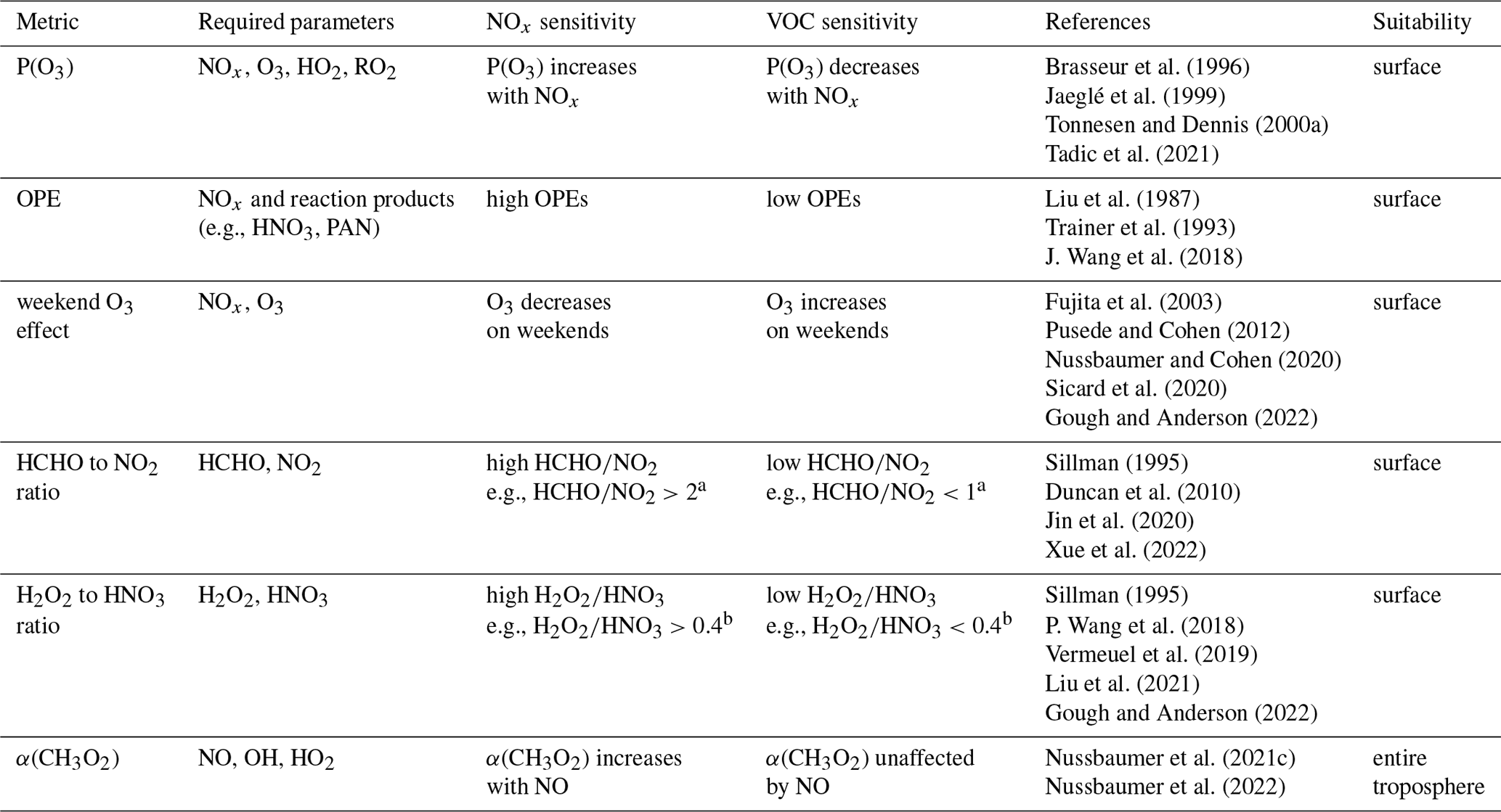
a Duncan et al. (2010). b Sillman (1995).
Some studies have directly addressed the production of O3 (or odd oxygen (Ox) ≡ O3 + NO2) in response to changing NOx (Brasseur et al., 1996; Jaeglé et al., 1999; Tonnesen and Dennis, 2000a; Tadic et al., 2021). Other studies have considered the so-called ozone production efficiency (OPE), which evaluates how many ozone molecules are formed by NOx before it is removed and transformed into reaction products such as HNO3 or peroxyacetyl nitrate (PAN) (Liu et al., 1987; Trainer et al., 1993; J. Wang et al., 2018). Low OPEs indicate a VOC-sensitive regime and high OPEs a NOx-sensitive regime. Similar approaches such as the ratio of O3 and reactive nitrogen species (NOy) or NOz (≡ NOy − NOx) have also been reported (Milford et al., 1994; Sillman, 1995; Fischer et al., 2003; Peralta et al., 2021; P. Wang et al., 2022).
A common method for determining the dominant regime in urban environments is the weekend ozone effect, where the response of O3 levels to decreasing NOx mixing ratios on weekends is monitored (e.g., Fujita et al., 2003; Pusede and Cohen, 2012; Nussbaumer and Cohen, 2020; Sicard et al., 2020; Gough and Anderson, 2022).
Another indicator is the ratio between formaldehyde (HCHO) and NO2. Sillman (1995) originally suggested the (NOy ≡ NOx + HNO3 + organic nitrates) ratio as a metric, which was later adjusted to the ratio. This metric evaluates the reaction of OH radicals with VOCs (ultimately leading to HCHO as a reaction intermediate) enhancing O3 production in competition with the reaction of OH radicals with NO2, which decelerates O3 formation (Tonnesen and Dennis, 2000b). The ratio has been widely applied in the literature based on ground-based measurements and satellite observations (e.g., Duncan et al., 2010; Jin et al., 2020; Xue et al., 2022).
The ratio of hydrogen peroxide (H2O2) to HNO3 is another metric used for regime analysis. Also initially suggested by Sillman (1995), it compares the HO2 self-reaction (forming H2O2) with the reaction of OH and NO2, both leading to termination of the HOx cycle. While the HO2 self-reaction dominates over the formation of HNO3 as a termination reaction, O3 increases linearly with NOx. Recent studies using include P. Wang et al. (2018), Vermeuel et al. (2019) and Liu et al. (2021). The and ratios, as well as the OPE, require absolute values as reference points to determine the regime, which can vary depending on the ambient conditions; background mixing ratios are a major drawback of these metrics.
Dyson et al. (2023) recently analyzed the dominant regime in Beijing using a method that considers the loss of OH, HO2 and RO2 radicals via reaction with NOx in comparison to the overall production of these radical species. The production thereby equals the overall radical loss via reaction with NOx, self-reaction and aerosol uptake, an idea which has been previously described by Sakamoto et al. (2019). Within a VOC-sensitive regime, HO2 is predominantly lost via the reaction with NO, while in a NOx-sensitive regime, aerosol uptake plays a significant role in HO2 loss. Dyson et al. (2023) found the transition to occur around 0.1 ppbv of NO.
Cazorla and Brune (2010) and Hao et al. (2023) reported direct measurements of P(O3) in a reaction chamber through observing changes in Ox in a certain time interval. This technique can be used to determine the dominant chemical regime when correlated with ambient NO mixing ratios.
These metrics were developed for the conditions near the surface, and most of them have not been applied to higher altitudes in the troposphere. Of the above metrics, the HCHO to NO2 ratio is the only one that we find to be applicable to high altitudes as well – but only in combination with ambient NO mixing ratios. We demonstrate this in Sect. 3.3. So far, absolute thresholds (e.g., lower than 1 for VOC sensitivity or higher than 2 for NOx sensitivity; Duncan et al., 2010) have been reported and applied in the literature. Due to the strong vertical trace gas gradients, these absolute thresholds are not applicable in the upper troposphere.
Some studies (including Jaeglé et al., 1998; Wennberg et al., 1998; Jaeglé et al., 1999) have analyzed the dominant chemical regime in the UT. These studies focus on the US and the North Atlantic and consistently report a linear correlation between P(O3) and NOx based on aircraft observations, deducing a NOx-sensitive regime, while model simulations predict a P(O3) decrease with high NOx. One explanation for these observations could be that these studies, published around 25 years ago, overestimated the NOx loss. We know today that the reaction rate of NO2 and OH is much lower than previously assumed (Mollner et al., 2010; Henderson et al., 2012; Nault et al., 2016). The loss reaction of NO2 with OH to HNO3 does not play a significant role under the conditions in the upper troposphere (in contrast to low altitudes) so that the typical definition for a VOC-sensitive regime where O3 production decreases with increasing NOx does not apply anymore. Khodayari et al. (2018) reported a NOx-saturated (VOC-sensitive) regime based on a modeling sensitivity study, where globally a decreasing O3 burden was observed with increasing lightning NOx. We suggest that this observed anti-correlation might not result from increased NOx loss as is applicable for surface conditions and might instead be an outcome of decreasing HO2 with increasing NO. Pickering et al. (1990) reported a VOC-sensitive regime over the USA at 11 km altitude based on measurements in June 1985 and model simulations. A study by Dahlmann et al. (2011) indicates increasing P(O3) with increasing NO at 250 hPa over Europe, implying a NOx-sensitive regime following the common definition. Shah et al. (2023) analyzed the relationship between the NOy/NO ratio and O3 mixing ratios and assumed a NOx-sensitive regime over the central US based on a flight during the DC3 research campaign in 2012. Liang et al. (2011) analyzed changes in net ozone production with NOx in the Arctic troposphere and found a proportional relationship up to 10 ppbv NOx based on box model calculations and observations.
While all studies have briefly touched upon the dominant chemical regime in the upper troposphere, a thorough analysis and a definition that is valid throughout the troposphere have not yet been reported. In view of ozone's major implications for the earth's radiative energy budget and climate change (particularly in the UT), O3 sensitivity is highly relevant for understanding and monitoring which precursors and processes are most important for the O3 budget at high altitudes in the troposphere.
In Nussbaumer et al. (2021a), we introduced a new metric α(CH3O2) for determining the dominant regime, which presents the ratio of methyl peroxy radicals (CH3O2) forming HCHO with NO versus the reaction of CH3O2 with HO2. We have applied this metric to ground-based observations at three different sites in Europe and for aircraft observations during the 2022 BLUESKY research campaign in the upper troposphere over Europe (Nussbaumer et al., 2022). We found a change at high altitudes from a VOC- to a NOx-sensitive regime over the past 2 decades up to 2020, promoted by emission reductions during the COVID-19 pandemic.
In this study, we use α(CH3O2) to analyze the dominant regime in the upper tropical troposphere between 30∘ S and 30∘ N latitude based on modeled trace gas mixing ratios and meteorological parameters by the ECHAM5/MESSy2 Atmospheric Chemistry (EMAC) general circulation model. We additionally investigate the effects of NOx produced by lightning in six different tropical areas: the Pacific Ocean, South America, the Atlantic Ocean, Africa, the Indian Ocean and South East Asia. Finally, we provide a new definition for NOx- and VOC-sensitive regimes, which is valid throughout the troposphere.
2.1 Calculations of ozone production (P(O3)) and loss (L(O3)) rates
The calculation of ozone production (P(O3)) and loss (L(O3)) rates was performed as presented in Sect. 2.1 of Nussbaumer et al. (2022). Briefly, ozone production P(O3) is described by the reaction of NO with HO2 and peroxy radicals RzO2 (Eq. 1); the latter can be approximated by CH3O2 in the upper troposphere. CH3O2 accounts for 85±5 % of RzO2, represented by the sum of CH3O2, C2H5O2 (ethyl peroxy radicals), CH3CO3 (peroxyacetyl radicals), CH3COCH2O2 (acetonyl peroxy radicals), iso-C3H7O2 (isopropyl peroxy radicals), C5H6O3 (isoprene (hydroxy) peroxy radicals), C4H7O4 (methyl vinyl ketone/methacrolein peroxy radicals) and LHOC3H6O2 (hydroxy peroxy radicals from propene + OH).
Ozone loss L(O3) is calculated as shown in Eq. (2) via the reaction of O3 with HO2 and OH and via photolysis. The latter only yields an effective ozone loss if O(1D) (resulting from O3 photolytic cleavage) reacts with H2O instead of colliding with O2 or N2 (and reforming O3). This share is represented by in Eq. (3).
The resulting net ozone production rate (NOPR) is then calculated by subtracting ozone loss from its production as shown in Eq. (4).
2.2 Calculations of α(CH3O2)
α(CH3O2) represents the share of methyl peroxy radicals forming HCHO with NO and OH versus the reaction with HO2 yielding CH3OOH and is calculated as shown in Eq. (5).
We demonstrated in previous studies that α(CH3O2) can be used as a metric to determine the dominant chemical regime (Nussbaumer et al., 2021a, 2022). The formation of HCHO from CH3O2 through reaction with NO leads to O3 formation, as NO2 is formed simultaneously, which can subsequently react to O3 via photolysis. In contrast, the reaction of CH3O2 with HO2 represents a termination reaction of the HOx cycle and therefore decelerates P(O3). CH3O2 is here a proxy for VOCs which form HCHO and O3 through RO2. A principal precursor to CH3O2 is CH4, which is oxidized by OH radicals and reacts with O2 in the first two steps of the catalytic HOx cycle. The atmospheric CH4 concentration is increasing rapidly, with the tropics implicated, suggestive of feedbacks that may accelerate CH4 growth in the future, contributing to O3 formation in the upper troposphere (Griffiths et al., 2021; Nisbet et al., 2023). Other precursors to CH3O2 can be acetone, methyl hydroxy peroxide or acetaldehyde through photolysis or reaction with OH radicals (Nussbaumer et al., 2021a). The advantage of considering CH3O2 is that it represents an entire group of VOCs that can form O3, including CH4, instead of handling multiple trace gases and risking incompleteness. The progression of α(CH3O2) in dependence of the ambient NO mixing ratio is shown in Fig. 1. The black line presents the average α(CH3O2) across all longitudes and between 30∘ S and 30∘ N latitude at 200 hPa altitude for daily values from 2000 to 2019 binned to the NO mixing ratios, as obtained from the EMAC modeling output. It therefore describes the background behavior of NO vs. α(CH3O2) for all data used in this study. The grey error shades show the 1σ standard deviation resulting from the averaging. At low NO mixing ratios (here <0.1 ppbv), α(CH3O2) changes rapidly even with small changes in NO. The resulting slope of the linear fit of the data is 3.75±0.44 ppbv−1. In this range, CH3O2 reacts both with NO and with HO2 (and with itself). With increasing availability of NO, the reaction of CH3O2 with NO and therefore the amount of O3 formed is enhanced. This regime is referred to as NOx-sensitive. In comparison, for higher NO mixing ratios (here >0.1 ppbv), α(CH3O2) only shows minor changes with increasing NO and is almost constant. The resulting slope is 0.16±0.01 ppbv−1. In this range, NO is so abundant that CH3O2 reacts primarily with NO, and changes in NO have almost no impact on the reaction. The amount of O3 formed is limited by the abundance of CH3O2, which itself is formed by a precursor VOC, and no longer increases with increasing NO. This regime is referred to as VOC-sensitive. Depending on where in this graph the data points from specific areas are located, it is possible to identify if a NOx- or a VOC-sensitive regime is dominant. This method underlines that O3 sensitivity is dependent on the availability of NO and HO2 radicals. Individual VOCs do not need to be considered when investigating O3 sensitivity, as HO2 effectively represents their chemical impact.
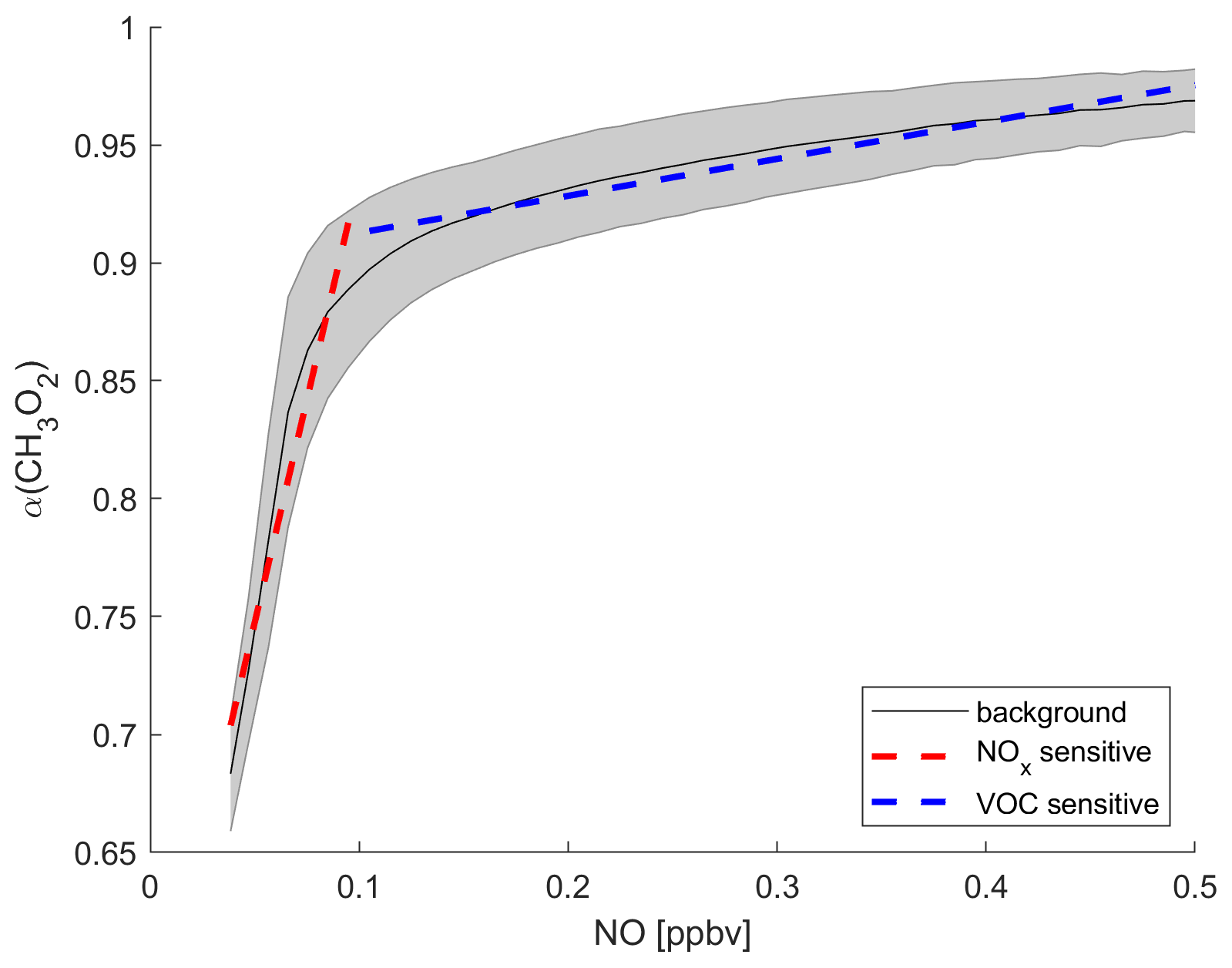
Figure 1Illustration of how α(CH3O2) can serve as a metric to determine the dominant chemical regime. The black line shows the tropical background α(CH3O2) binned to NO mixing ratios from the EMAC model output. The grey shading shows the 1σ standard deviation. The dashed red line is a linear fit for NO < 0.1 ppbv and represents NOx-sensitive O3 chemistry. The dashed blue line represents VOC-sensitive O3 chemistry for NO > 0.1 ppbv.
2.3 Modeling study
The data analyzed in this study were produced by model simulations using the ECHAM5 (fifth-generation European Centre Hamburg general circulation model, version 5.3.02)/MESSy2 (second-generation Modular Earth Submodel System, version 2.54.0) Atmospheric Chemistry (EMAC) model. Details on the EMAC model can be found in Jöckel et al. (2016). We applied EMAC in the T63L47MA resolution, i.e., with a spherical truncation of T63 (corresponding to a quadratic Gaussian grid of 1.875∘ by 1.875∘ in latitude and longitude) with 47 vertical hybrid pressure levels up to 0.01 hPa. Roughly 22 levels are included in the troposphere depending on the latitude, and the model has a time step of 6 min. The dynamics of the EMAC model have been weakly nudged in the troposphere (Jeuken et al., 1996) towards the ERA5 meteorological reanalysis data (Hersbach et al., 2020) of the European Centre for Medium-Range Weather Forecasts (ECMWF) to represent the actual day-to-day meteorology in the troposphere. The setup adopted here is similar to the one presented in Reifenberg et al. (2022), using the anthropogenic emissions CAMS-GLOB-ANTv4.2 (Granier et al., 2019), with varying monthly values for the period 2000–2019. The model has been extensively evaluated for ozone (e.g., Jöckel et al., 2016), showing a systematic though minor overestimation of the model compared to observations, which is a common feature in chemistry general circulation models of this complexity (Young et al., 2013). Comparison of the model results against numerous field campaigns (e.g., Lelieveld et al., 2018; Tadic et al., 2021; Nussbaumer et al., 2022) reveals a good agreement between observations and model results of NOx and VOCs for locations in the UT. The reference simulation covers the time period 2000–2019 with hourly output of trace gas mixing ratios of O3, NO, NO2, OH, HO2, CH3O2, HCHO, CO, CH4 and H2O, as well as the photolysis rates j(NO2) and j(O1D) and meteorological parameters such as temperature and pressure, necessary for calculating net ozone production rates and α(CH3O2). The data were post-processed to obtain daily values at local noon time and were calculated for 200 hPa (upper troposphere) using bilinear interpolation between the hybrid pressure model levels. This pressure level was chosen to represent upper tropospheric influence in the tropics in order to capture lightning events and avoid strong influence of transport from the stratosphere. The choice is also underlined by the results presented in Fig. 7 where 200 hPa marks the area of transition from NOx sensitivity in the free troposphere to VOC sensitivity in the stratosphere, impacted by lightning.
In this work the emissions of NOx from lightning follow the work of Tost et al. (2007). A constant NOx emission of ∼20.6 kg N per flash is used for cloud-to-ground flashes. The ratio of NOx production by intra-cloud flashes is lower by a factor of 0.1. The lightning frequency is estimated with the parameterization of Grewe et al. (2001). Here the updraft velocity (used as a proxy for convective strength) is associated with cloud electrification and is therefore proportional to the frequency of the lightning flashes. On the other side, aircraft emissions are prescribed from the CAMS dataset (CAMS-GLOB-AIR v1.1, Granier et al., 2019).
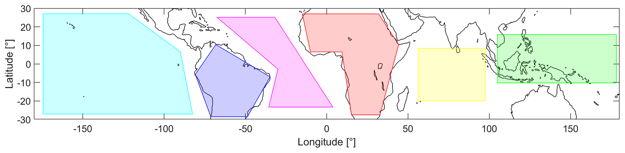
Figure 2Overview of the defined areas in the tropics between 30∘ S and 30∘ N latitude: Pacific Ocean (cyan), South America (blue), Atlantic Ocean (pink), Africa (red), Indian Ocean (yellow) and South East Asia (green).
For detailed analysis, six different areas are defined, and their geographic extent is shown in Fig. 2. These areas refer to the Pacific Ocean (cyan), South America (blue), the Atlantic Ocean (pink), Africa (red), the Indian Ocean (yellow) and South East Asia (green).
3.1 Development of trace gases over time
The analyzed trace gases do not show statistically significant trends over time from 2000 to 2019 at 200 hPa, which we show in Fig. S1 of the Supplement. We find small global increases of some trace gases, e.g., average NO and HO2 mixing ratios increase by ∼5 % and average NO2 and O3 mixing ratios by up to 10 % from 2000 to 2019. The global mean temperature increases by approximately 1 ∘C over the 20-year period. Even though slight trends can be detected, the variability is high, and the 1σ standard deviation (grey shaded) is significantly larger than the variation over time, and we therefore used a daily climatology from the 20-year period in order to simplify the calculations.
3.2 Tropical distribution
3.2.1 NOx
Figure 3 shows the distribution of NO in the upper tropical troposphere (at 200 hPa). We find large changes throughout the year related to the seasonality of deep convection and the location of the Intertropical Convergence Zone (ITCZ). Deep convection dominates in the Southern Hemisphere in January, and during July it is most prevalent in the Northern Hemisphere (Yan, 2005). In order to illustrate the differences, we subdivide the data into four periods, December–February (DJF), March–May (MAM), June–August (JJA) and September–November (SON). Each grid cell extends over latitude and longitude and represents a 20-year average of the respective period.
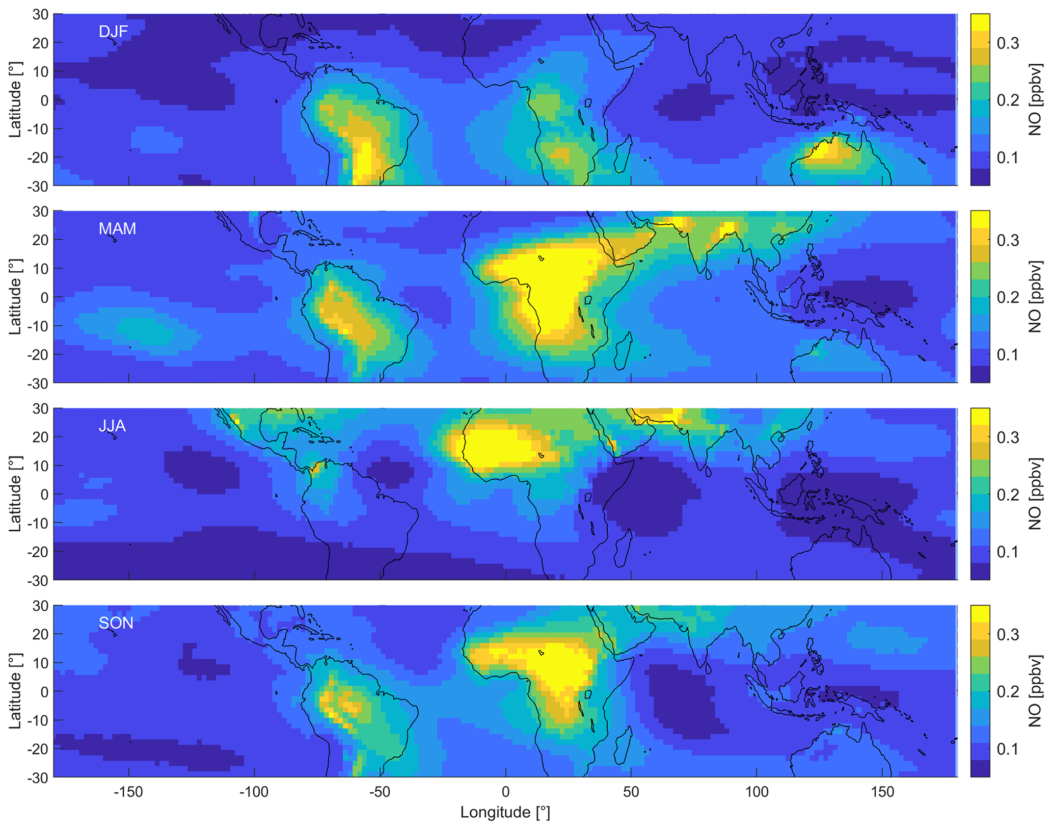
Figure 3Distribution of NO in the tropical UT between 30∘ S and 30∘ N during December–February (DJF), March–May (MAM), June–August (JJA) and September–November (SON).
During DJF, NO mixing ratios are the highest over the tropical continental areas of South America, southern Africa and northern Australia, with average peak values between 0.3 and 0.4 ppbv. In comparison, NO mixing ratios are much lower over the Pacific and the Indian oceans (0.09±0.01 ppbv), the Atlantic Ocean (0.12±0.02 ppbv), northern Africa (0.10±0.03 ppbv), and South East Asia (0.08±0.01 ppbv). Generally, the mixing ratios over land are much higher than those over the ocean, and the mixing ratios north of the Equator (0.09±0.03 ppbv) are lower compared to south of the Equator (0.14±0.06 ppbv). During MAM, NO mixing ratios over South America are similar to those during DJF (0.21±0.05 ppbv). NO mixing ratios over Africa are almost twice as high on average compared to DJF and reach peak values of 0.53 ppbv. The relative maxima relocate from southern to central Africa from DJF to MAM and also over the Arabian Peninsula and southern Asia, including India. Mixing ratios over Australia are around 0.15 ppbv and approximately half of those during DJF and are similar over South East Asia. During JJA, peak NO mixing ratios are found north of the Equator over central America and northern Africa. Average NO mixing ratios are almost 60 % higher in the tropical Northern Hemisphere (0.14±0.07 ppbv) compared to the tropical Southern Hemisphere (0.09±0.02 ppbv). The distribution, therefore, differs drastically from DJF. During SON, NO mixing ratios are similar to MAM and peak over South America and central Africa.
The highest NO mixing ratios are found in the locations of predominant deep convection, which vary throughout the year. In July, deep convection is the highest over central America, northern Africa and southern Asia (northern India). In January, it is predominant over South America, central to southern Africa and northern Australia (Yan, 2005). The areas where these convective processes are prevailing define the ITCZ where north- and southeasterly trade winds converge. Increased thunderstorm activity explains the occurrence of peak NO mixing ratios. Various studies have reported significantly increased lightning over land compared to the ocean, which is in line with the distribution of NO as shown in Fig. 3 (Christian et al., 2003; Rudlosky and Virts, 2021; Nussbaumer et al., 2021c). South East Asia is often referred to as the “maritime” continent. This region experiences frequent cumulonimbus activity, but the convective available potential energy (CAPE) is less compared with that over the South American and in particular the African land masses. This region therefore shows lower NO mixing ratios throughout the year. The relative distribution of NO2 is very similar to NO, which we show in Fig. S2. On average, NO2 mixing ratios are around a factor of 7 lower compared to NO.
3.2.2 HO2
Figure 4 shows the DJF and JJA distributions of HO2. An overview of all four periods can be found in Fig. S3. Similar to NO, the spatial DJF distributions of HO2 mixing ratios show peak values between 15 and 20 pptv over South America and southern Africa. While NO shows minimum values over South East Asia and the Indian Ocean, HO2 mixing ratios are elevated in these areas (12–13 pptv). Mixing ratios are lower over the Pacific and the Atlantic oceans (8–9±1 pptv) and north of ∼20∘ N. During JJA, HO2 mixing ratios are elevated over the Indian Ocean, South Asia and central America, including the Atlantic and Pacific oceans around 10∘ N latitude. HO2 is relatively low over South America and Africa. During MAM and SON, HO2 is mostly intermediate between DJF and JJA and does not show any noteworthy features. Mixing ratios of CH3O2 show a very similar distribution to HO2 across the tropical UT and range from ∼0.5 to 4 pptv, which we show in Fig. S4.
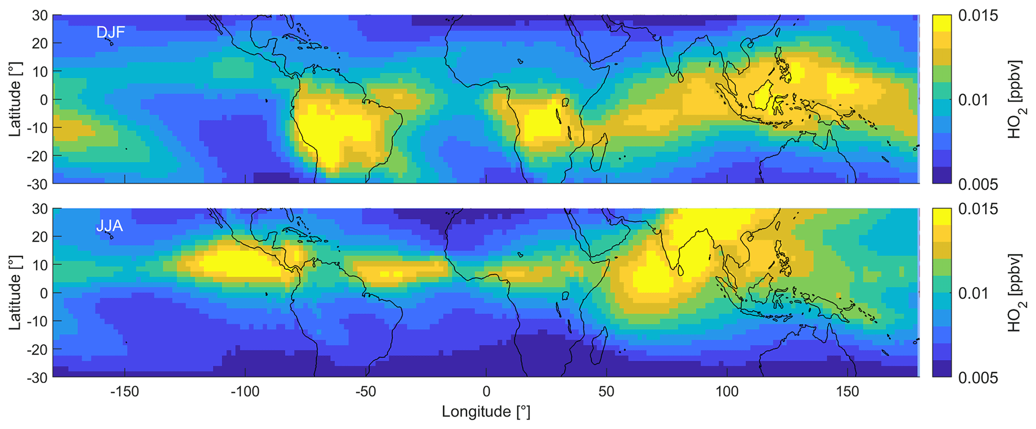
Figure 4Distribution of HO2 in the tropical UT between 30∘ S and 30∘ N during DJF and JJA.
3.2.3 NOPR
The tropical UT distribution of net ozone production rates is closely related to the distribution of NO (Fig. 3). We show the model-calculated results for each period in Fig. S5. During DJF, NOPRs peak over South America with average values of 0.77±0.20 ppbv h−1 and maximum values above 1 ppbv h−1 over southern Africa and northern Australia. During the course of the year, with local variations in deep convection, NOPR peaks move northwards, reaching the northernmost point in JJA, and move southwards again in SON and DJF. During DJF, NOPRs are almost 60 % higher in the Southern Hemisphere (0.36±0.21 ppbv h−1) compared to the tropical Northern Hemisphere (0.23±0.09 ppbv h−1). In contrast, during JJA, NOPRs are more than twice as high in the Northern Hemisphere (0.36±0.15 ppbv h−1) compared to the tropical Southern Hemisphere (0.17±0.06 ppbv h−1). The production of O3 outweighs its loss by a factor of 8 on average for the studied conditions. The difference is larger in regions with peak NOPRs, e.g., over South America with a factor of 11, and smaller in regions with low NOPRs, e.g., over the Pacific Ocean with a factor of around 7. We show the distribution of both P(O3) and L(O3) in Figs. S6 and S7. These results, showing similar features for NOPRs and NO geographically, are in line with findings by Apel et al. (2015), who reported enhanced ozone production for high lightning NOx over the US during a research flight in June 2012 as part of the DC3 campaign.
3.2.4 α(CH3O2)
Figure 5 shows the distribution of α(CH3O2) in the tropical UT during DJF and JJA. We show all periods in Fig. S8. During DJF, α(CH3O2) ranges from 0.77 to 0.95, with the lowest values over South East Asia and the highest values over southern Africa and Australia. During JJA, the lowest values are obtained over South East Asia and the Indian Ocean as well as the Pacific and Atlantic oceans around 10∘ N latitude. Maximum values of up to 0.97 are reached over northern Africa and the Arabian Peninsula. Therefore, as expected, α(CH3O2) is proportional to NOPR and NOx mixing ratios and is anti-proportional to HO2 mixing ratios. At low ratios, increases in NO enhance α(CH3O2), while at high ratios, changes in NO have no or only a small effect. We discuss the implications of α(CH3O2) for the dominant chemical regime in the tropical UT and specific regions in the following section.
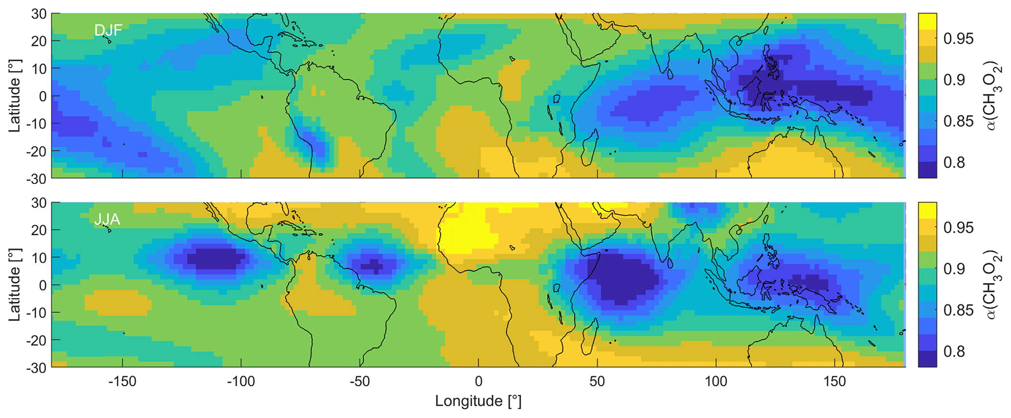
Figure 5Distribution of α(CH3O2) in the tropical UT between 30∘ S and 30∘ N during DJF and JJA.
3.3 Chemical regimes
3.3.1 Baseline scenario
Figure 6 presents α(CH3O2), O3 and the ratio binned to NO mixing ratios during DJF, MAM, JJA and SON. The graphs show NO mixing ratios up to 0.5 ppbv, which includes 99.6 % of all data points. The frequency distribution of the NO data can be seen in Fig. S9. The black lines and the grey shades represent the average of all data points binned to NO, which we refer to as the background, and the associated 1σ standard deviation. The colored data points show the averages of the individual areas as shown in Fig. 2. The error bars represent the 1σ variability. Data for the Pacific Ocean are shown in cyan, South America in blue, the Atlantic Ocean in magenta, Africa in red, the Indian Ocean in yellow and South East Asia in green. In this section, we first discuss the background curves (representing an average of all data points), and we subsequently present our findings for the individual areas.
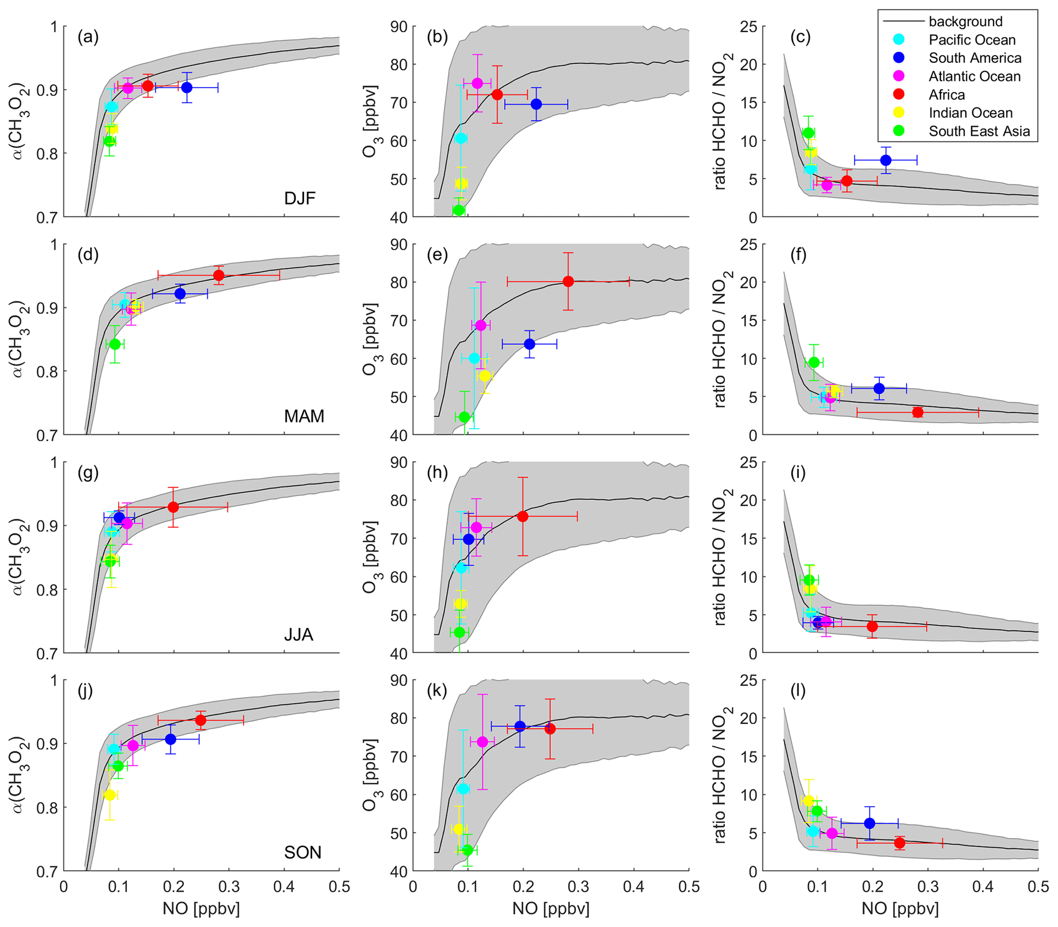
Figure 6Different metrics used to determine the dominant chemical regime. Left column: α(CH3O2), middle column: O3 and right column: the ratio, binned to NO mixing ratios for (a)–(c) December–February (DJF), (d)–(f) March–May (MAM), (g)–(i) June–August (JJA) and (j)–(l) September–November (SON). The black lines show the averages of all data points, and the grey shades present the 1σ standard deviation. The colored data points show the averages for the indicated areas and the 1σ variability.
Background α(CH3O2) (Fig. 6a, d, g and j) increases strongly with NO for mixing ratios below 0.1 ppbv with a slope of 3.75±0.44 ppbv−1. For example, an average increase of α(CH3O2) by 0.1 results from an increase of ambient NO by around 27 pptv. This characterizes the NOx-sensitive regime. In contrast, for NO mixing ratios higher than 0.1 ppbv NO, increasing NO has only a minor effect on α(CH3O2) (slope = 0.16±0.01 ppbv−1), which represents the VOC-sensitive regime. To reach an increase in α(CH3O2) by 0.1, ambient NO needs to increase by 625 pptv, a factor of >20 higher compared to the low-NOx regime. Within the NOx-sensitive regime, predominantly CH3O2 reacts with NO, forming O3, as well as with HO2, which does not result in formation of O3. With increasing NO, the share of the reaction with NO (compared to the reaction with HO2) increases, which in turn enhances O3. In contrast, within the VOC-sensitive regime CH3O2 radicals mostly react with NO in any case, and increases in NO do not affect O3. This is illustrated in the middle column of Fig. 6 (panels b, e, h and k): O3 increases with NO for low NO mixing ratios and reaches a plateau for high NO mixing ratios. While the shift from the NOx- to the VOC-sensitive regime is relatively sharp for α(CH3O2), the transition for O3 is broader and more difficult to relate to an NO mixing ratio. This graph is illustrative but should not be used solely for determining the dominant chemical regime. In the right column (Fig. 6c, f, i and l), we present the ratio binned to NO mixing ratios. In the literature, absolute values for the ratio are mostly used to determine the chemical regime, meaning the ratio is calculated and compared to a certain threshold, for example for NOx sensitivity and for VOC sensitivity (Duncan et al., 2010). These threshold values are not valid in the upper troposphere due to the vertical gradients of the trace gases. However, the ratio can also indicate the transition from a NOx- to a VOC-sensitive regime when binned to NO mixing ratios, which does not require any absolute threshold values. Within the NOx-sensitive regime, the ratio strongly decreases with small increases in NO, and within the VOC-sensitive regime it is mostly unresponsive to changes in NO. Depending on where in these plots a specific data point or an average of several data points is located, it is possible to derive the dominant chemical regime.
As explained earlier, it is not possible to determine the dominant chemical regime from ozone formation rates P(O3) in the upper troposphere, as the formation of HNO3 plays a minor role at UT altitudes and therefore does not lead to a decrease in P(O3), which in theory indicates the dominance of VOC over NOx sensitivity. In fact, P(O3) does decrease for NO mixing ratios above around 0.7 ppbv but for a different reason, as shown in Fig. S10. Figure S10a presents P(O3) binned to NO, which increases for low NO, reaches a plateau around 0.6–0.7 ppbv NO and decreases at higher NO. Figure S10b shows NOx loss (L(NOx)) rates via OH, HO2 and CH3O2, which are negligible compared to P(O3) rates as shown in Fig. S10a. Even though L(NOx) increases with increasing NO, it is still only 6 % of the ozone production at 1 ppbv NO. The decrease in P(O3) is therefore not associated with the formation of HNO3 (as it is in the lower troposphere) but reflects the decrease of HO2 with increasing NO (see Fig. S10c and d). The peak in P(O3), therefore, does not provide an indication for a regime change.
To investigate individual areas regarding predominant O3 sensitivity, we analyze the location of the area averages along the background. Figure 6a shows NO vs. α(CH3O2) during DJF. The tropical UT over the Indian Ocean and South East Asia is characterized by NOx sensitivity with NO mixing ratios between 80 and 90 pptv and an average α of 0.84 and 0.82, respectively. Ozone formation over South America is VOC-sensitive with an average NO mixing ratio of 222 pptv and an α of 0.90. The data points for the Pacific Ocean, the Atlantic Ocean and Africa are close to the transition point of the two regimes, with a tendency of the Pacific Ocean towards NOx and of the Atlantic Ocean and Africa towards VOC sensitivity. This is in line with Fig. 6b, which presents NO vs. O3 mixing ratios. The data points for South East Asia, the Indian Ocean and the Pacific Ocean are mostly located in the upsloping part of the curve, where O3 strongly increases with increasing NO. The averages for the Atlantic Ocean, Africa and South America are located towards the flattening of the curve. Figure 6c shows the DJF averages for NO vs. the ratio. For South East Asia, the Indian Ocean and the Pacific Ocean, NO mixing ratios are below 0.1 ppbv and ratios are high with values of 6.3, 8.5 and 10.9 ppbv ppbv−1, respectively. For the Atlantic Ocean and Africa, the average NO mixing ratios are higher and the ratios are lower with values of 4.2 and 4.7 ppbv ppbv−1, respectively. NO mixing ratios over South America are even higher, but the ratio is also higher with a value of 7.4 ppbv ppbv−1. This underlines the limitation of using absolute threshold values for determining the dominant chemical regime. If a threshold for the regime transition was to be set to, e.g., 5 ppbv ppbv−1, the South American UT would be characterized as NOx-sensitive, while it clearly shows VOC sensitivity. It is therefore important to consider the metrics used in relation to ambient NO mixing ratios, and it is best to use them in combination with other metrics.
Figure 6d shows α(CH3O2) binned to NO for MAM data. The UT over South East Asia is NOx-sensitive with values similar to DJF. Over the Indian Ocean, both the average NO mixing ratio and α(CH3O2) increase to 130 pptv and 0.90, respectively, being located in the transition regime, together with the Pacific Ocean and the Indian Ocean. Minor changes from DJF to MAM occur over South America, which is still VOC-sensitive. A strong VOC sensitivity is calculated for the UT over Africa with average NO mixing ratios of 279 pptv and α(CH3O2) of 0.95. These findings are confirmed by O3 and the ratio binned to NO in Fig. 6e and f. The data for South East Asia, the Pacific Ocean, the Atlantic Ocean and South America are similar to the values during DJF. Between DJF and MAM, the values over the Indian Ocean and Africa change to higher NO (131 and 279 pptv) in combination with higher O3 (55 and 80 ppbv) and a lower ratio (5.7 and 3.0 ppbv ppbv−1), associated with a change from the NOx-sensitive regime to the transition regime and a change from the transition regime to the VOC-sensitive regime, respectively.
Figure 6g–i show similar graphs for June–August (JJA), indicating NOx sensitivity for the UT over South East Asia and the Indian Ocean; a transition regime for the Pacific Ocean, the Atlantic Ocean, and South America; and VOC sensitivity for Africa. During September–November (SON), as shown in Fig. 6j–l, South America shifts back to VOC sensitivity. All other regimes remain unchanged between JJA and SON.
Figure S11 shows the mean values of the specified areas for P(O3) vs. NO. While the computational tools presented above allow for a clear distinction between the regimes depending on the location and time of the year, this indicator shows no differences. According to the surface-oriented definition for chemical regimes, all data points would be located in the NOx-sensitive regime.
In summary, Fig. 6 illustrates three important results. First, the transition between NOx and VOC sensitivity occurs at around 0.1 ppbv NO in the upper tropical troposphere. Second, areas with increased lightning activity tend towards the dominance of VOC sensitivity. And third, the dominating regime changes with the time of the year. We discuss these findings and their implications in the following.
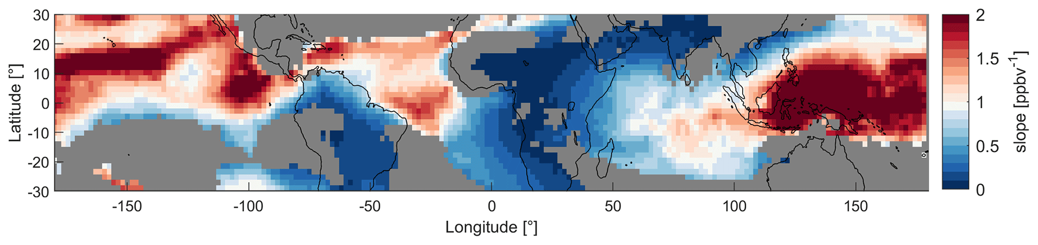
Figure 7Map of the tropical UT between 30∘ S and 30∘ N colored by the slopes of NO vs. α(CH3O2) of the data in the model grid regions during MAM. The red colors indicate NOx sensitivity and the blue colors VOC sensitivity. For the grey areas the R2 of the fit is below 30 %.
Since NO and HO2 mixing ratios, as well as NOPRs, change throughout the year, the varying locations of deep convection also affect the dominant chemical regime. Areas with deep convection are potentially associated with lightning activity, resulting in higher NO mixing ratios that lead to VOC sensitivity. The continental areas of South America and especially Africa experience most lightning and therefore show the most VOC-sensitive regimes (Williams and Sátori, 2004). As the cumulonimbus clouds in South East Asia are mostly formed in maritime conditions, the region experiences significantly less lightning and therefore shows NOx sensitivity year-round. Ozone formation over the oceans is either NOx-sensitive or in the transition regime as lightning strikes are significantly less frequent in maritime areas compared to continental areas. Figure 7 presents a geographical distribution of the tropical UT colored by the slopes of the NO vs. α(CH3O2) data in each individual grid region to illustrate the dominating chemical regimes. Here, we present a map for MAM data. In Fig. S12, we show them for all periods. High values for the slopes and red colors (i.e., values well above 1) represent the predominantly NOx-sensitive regime, and low values, accompanied by blue colors, represent VOC sensitivity. It is not possible to determine an exact threshold slope for the transitioning between regimes. Generally, the more intense the color (red or blue), the more clearly a location is assigned to one of the two regimes. Lighter colors indicate a state closer to the transition regime. Grey areas indicate that the R2 of the fit is <30 %, which, for example, occurs when the data are arranged in a cloud of points. This depiction is in line with the results from Fig. 6. During MAM, the blue colors over South America and Africa indicate a VOC-sensitive regime. The red colors over South East Asia show NOx sensitivity. Finally, over the three oceans we find lighter colors indicating the transition regime. This view also allows for a more detailed differentiation between the areas; for example, the UT over the Atlantic Ocean tends more towards a NOx-sensitive regime in the northern part and towards a VOC-sensitive regime in the southern part.
While we focus on the upper troposphere in this study, α(CH3O2) remains a suitable indicator of the dominant chemical regime at all altitudes. In Fig. 8 we present the slopes of NO vs. α(CH3O2) by pressure altitude and longitudes, as an example for MAM data close to the Equator (1∘ N). The white areas at the bottom (between 800 and 1000 hPa) result from the local surface topography (mountains). For the free troposphere, we find strong NOx sensitivity with a maximum slope of 38 ppbv−1. In the upper troposphere–lower stratosphere at pressure altitudes between 300 and 100 hPa, we observe the transitioning to a VOC-sensitive regime. For latitudes with strong lightning activity, including areas such as continental South America (−80 to −60∘ longitude) and Africa (5 to 30∘ longitude), the transition occurs in the upper troposphere, corresponding to pressure altitudes of 250–300 hPa. For latitudes with low lightning activity, for example, between 130 and 160∘ longitude (South East Asia), the regime change only occurs at the transition to the lower stratosphere – at a pressure altitude of around 150 hPa – which is characterized by strong NOx saturation. In Fig. S13 we additionally show the dominant chemical regime, indicated by NO vs. α(CH3O2), on a global scale near the surface as the annual average. As we would expect, α(CH3O2) indicates VOC sensitivity at the surface for all urbanized and industrialized regions characterized by high NOx emissions and NOx sensitivity for remote regions. Shipping routes, which are closer to the transition regime, can be distinguished from the pronounced maritime NOx sensitivity.
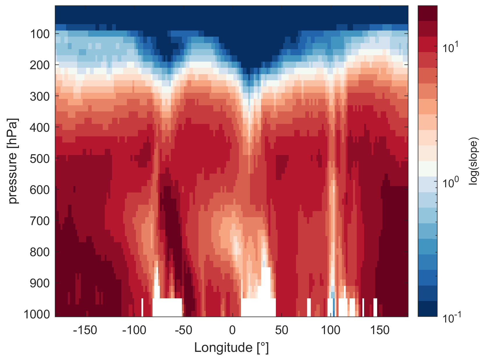
Figure 8Slopes of NO vs. α(CH3O2) by pressure altitude and longitude on a log scale during the March–May (MAM) period and close to the Equator (1∘ N). The red colors indicate NOx sensitivity and the blue colors VOC sensitivity. The white areas between 800 and 1000 hPa result from the local surface topography.
3.3.2 Sensitivity study: lightning NOx
Three additional model runs were performed in order to investigate the impact of lightning NOx. First, lightning NOx was completely omitted. In the second and third runs, NOx from lightning was halved and doubled, respectively, compared to the baseline scenario. The emissions of global lightning NOx in the baseline scenario amount to 6.2 Tg yr−1 (estimated from the climatological data), in agreement with the work of Miyazaki et al. (2014).
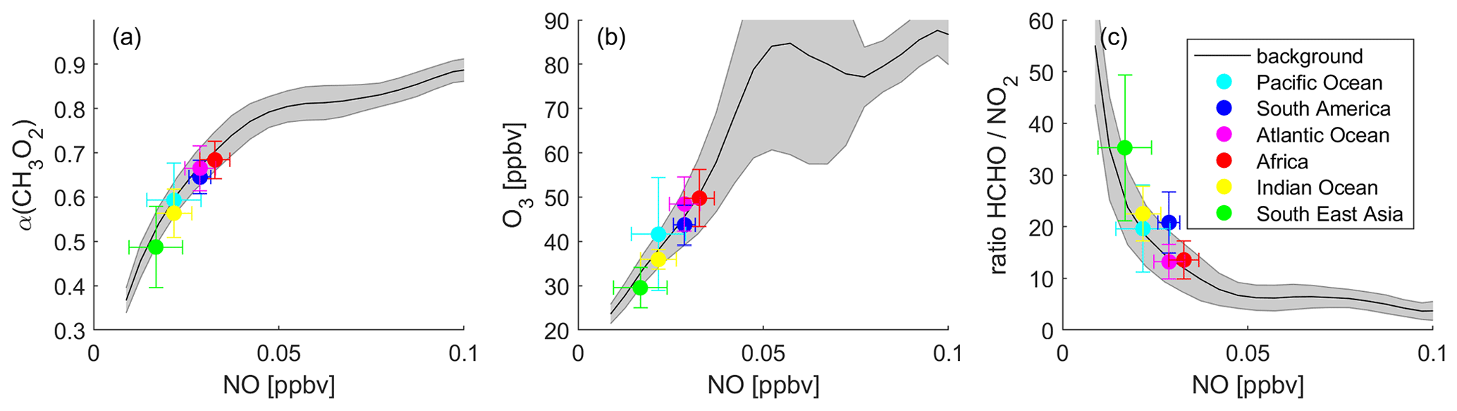
Figure 9Determination of the dominant chemical regime in the tropical UT in the “no lightning” scenario via (a) α(CH3O2), (b) O3 and (c) the ratio, binned to NO mixing ratios. The black lines show the averages of all data points, and the grey shades present the 1σ standard deviation. The colored data points show the averages for the indicated areas with the 1σ variability.
Figure 9 shows the three previously discussed metrics, α(CH3O2) (Fig. 9a), O3 (Fig. 9b) and the ratio (Fig. 9c), binned to NO mixing ratios for the modeling scenario excluding lightning NOx. As there are no significant differences between the periods, we show all-year data here. Figure S14 shows the subdivision into the four periods (DJF, MAM, JJA and SON), and in Fig. S15, we present a comparison between the baseline scenario as a yearly average and the scenario excluding lightning. The black lines representing the average of all data points show a similar course compared to the baseline scenario including lightning NOx, but the distinction between the regimes is less pronounced. Figure 9a presents NO vs. α(CH3O2). At low NO mixing ratios, α(CH3O2) increases with NO, indicating NOx sensitivity, and for higher NO mixing ratios, α(CH3O2) is only marginally affected by changes in NO, indicating VOC sensitivity. The tropical UT over all selected areas is clearly located within the NOx-sensitive chemical regime. The average NO mixing ratios range from 17 pptv over South East Asia to 33 pptv over Africa. Compared to the baseline scenario, excluding lightning NOx leads to a decrease in ambient NO levels by up to 1 order of magnitude. The average α(CH3O2) ranges from 0.49 to 0.68 over South East Asia and Africa, respectively. The abundance of HO2 in comparison to NO is therefore high, and a significant amount of CH3O2 undergoes reaction with HO2, next to NO. Figure 9b shows the O3 mixing ratios as a function of NO. The O3 mixing ratios first increase as a function of NO, reach a peak at around 0.05 ppbv NO and 85 ppbv O3, and subsequently change little at higher NO levels. Note that the number of data points decreases rapidly for high NO mixing ratios. Only around 5.5 % of the data points represent NO values of >0.05 ppbv. We show the associated frequency distribution in Fig. S16. As expected, the data points of all selected areas are located at low NO and O3 levels, at average O3 mixing ratios ranging from 30 ppbv over South East Asia to 50 ppbv over Africa. Figure 9c shows the ratio binned to NO mixing ratios. The course of the average values (black line) is again similar to the one for the baseline scenario, but the values for the ratio are higher. The highest average value occurs over South East Asia with 35.2 ppbv ppbv−1 and the lowest over the Atlantic Ocean with 13.2 ppbv ppbv−1. All data points are therefore clearly located within the NOx-sensitive regime, which is in line with the findings from the correlation between NO and α(CH3O2) from Fig. 9a.
In Figs. S17 and S18, we present the three metrics α(CH3O2), O3 and the ratio binned to NO mixing ratios for all periods and locations for halved and doubled lightning NOx, respectively. The transition region between the regimes occurs around 0.1 ppbv and is therefore not meaningfully different from that in the baseline scenario, but the distinction between the regimes is more conspicuous with increasing lightning NOx emissions.
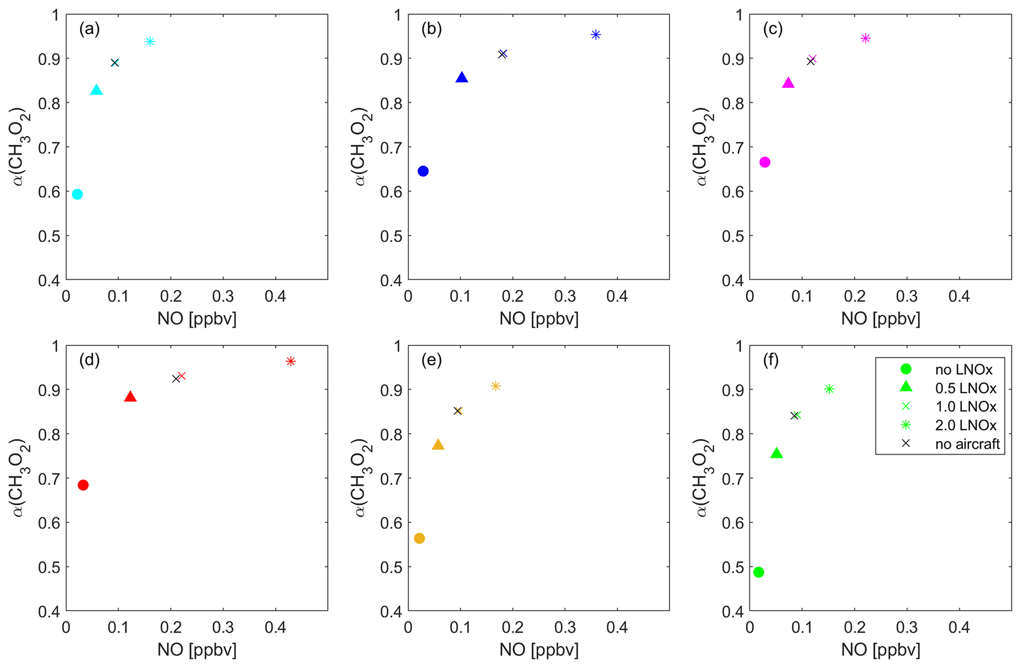
Figure 10Overview of the impact of lightning NOx on the dominant O3 sensitivity. The data points present the average NO vs. α(CH3O2) of all data points located in each of the six regions: (a) the Pacific Ocean (cyan), (b) South America (blue), (c) the Atlantic Ocean (pink), (d) Africa (red), (e) the Indian Ocean (yellow) and (f) South East Asia (green) for the baseline scenario (crosses), excluding lightning (circles), halved lightning (triangles) and doubled lightning (asterisks).
Figure 10 shows the average α(CH3O2) vs. NO for each considered location and for all modeled lightning NOx scenarios. As expected, in each location the data points shift to higher values for both NO and α(CH3O2) with increasing influence of lightning NOx. When excluding lightning, the dominant regime changes to NOx-sensitive in all locations. Removing lightning also shows that lightning is by far the dominant source of NOx in the upper tropical troposphere. In maritime regions where lightning is relatively infrequent, NOx more strongly depends on advection from continental regions, formation from HNO3 and aircraft emissions. A model run excluding NOx emissions from aircraft does not lead to significant differences compared to the baseline scenario, which we present with the black crosses in Fig. 10. This may contradict recent findings by H. Wang et al. (2022), who presented increases in upper tropospheric ozone in response to increasing aircraft emissions. In our model, NOx in the tropical upper troposphere is dominated by lightning emissions, whereas NOx concentrations from aviation in this part of the troposphere are small, with most aircraft emissions occurring north of 30∘ N latitude. Excluding lightning shows that NOx mixing ratios also decrease significantly in maritime environments, including South East Asia where NOx mixing ratios drop from 90 to 17 pptv on average. This illustrates that in maritime locations in the tropics, i.e., apart from South America and central Africa, NOx mixing ratios are largely dependent on transported lightning NOx. For halved lightning NOx, NOx sensitivity also prevails in most locations. Only Africa and South America show a transition regime for the periods of the year with maximum lightning. For doubled lightning NOx, the qualitative regime observations are similar to the baseline scenario. The UT over central Africa and South America is mostly VOC-sensitive, over South East Asia and the Indian Ocean it is NOx sensitive, and this layer is in the transition regime over the Pacific and Atlantic Ocean. Therefore, regions with frequent lightning are VOC sensitive in the baseline scenario, while the doubling of lightning NOx does not have a large impact in regions where lightning is generally infrequent. In accordance with our prior analysis, O3 does not increase significantly from the doubling of lightning NOx. In the VOC-sensitive regime, the black curve representing the average of all data points of NO vs. O3 levels off at around 90 ppbv compared to 80 ppbv for the baseline scenario. This aids our understanding of NOx and VOC sensitivity in the upper troposphere, as all available HO2 and CH3O2 radicals react with NO within the VOC-sensitive regime, and changes in NOx therefore do not affect changes in O3.
The sensitivity study of lightning NOx emphasizes two major aspects. First, lightning is the predominant source of NOx in the upper tropical troposphere as the mixing ratios drop to near zero when excluding it, and a model run excluding aircraft NOx does not show significant differences compared to the baseline scenario. Second, lightning and its distribution in the tropics, which is affected by the partitioning of continental and maritime areas and the varying locations of deep convection throughout the year, are the most important determinants of the dominant chemical regime in the UT. Our results additionally indicate that any future changes in lightning will only significantly affect O3 levels in the upper troposphere if lightning substantially increases in locations where it is currently sparse or if lightning decreases in areas where it is presently frequent. Our results fit well with previous literature on the role of lightning NOx in O3 production in the upper troposphere. Grewe (2007) reported that NOx from lightning is the dominant source of O3 in the upper tropical troposphere based on simulations with the global climate–chemistry model E39/C. Similar results have been presented by Murray (2016), Schumann and Huntrieser (2007), and Sauvage et al. (2007). While it has been shown previously that ozone production in the upper tropical troposphere is highly dependent on lightning NOx, this study is the first to extensively study the impact of lightning on the dominant O3 regime, applying a new indicator α(CH3O2), which is valid throughout the entire troposphere.
We have investigated the dominance of NOx and VOC sensitivity in the upper tropical troposphere (200 hPa) between 30∘ S and 30∘ N latitude. The analyzed trace gas mixing ratios and meteorological parameters are calculated with the EMAC general circulation model for a horizontal resolution and the years 2000–2019. One model run considers a baseline scenario, and four additional ones were run with halved, doubled and excluded lightning NOx emissions, as well as excluded NOx aircraft emissions. We find that the mixing ratios of the considered trace gases have not changed significantly in the upper troposphere over the past 2 decades, and we therefore evaluate the average of the data which benefits from a higher statistical significance. The distribution of the analyzed trace gases varies with the time of the year and the changing areas of deep convection, confined within the ITCZ. During DJF, maximum convection occurs over South America, central to southern Africa and northern Australia and during JJA over central America, northern Africa and continental Asia. As a consequence, NOx mixing ratios and net ozone production rates peak over South America, southern Africa and northern Australia during DJF, over South America and central Africa during MAM and SON, and over central America and northern Africa during JJA, as deep convection brings increased thunderstorm and lightning activity, particularly over continental areas. The distribution of HO2 mostly differs from NOx due to enhanced mixing ratios over South East Asia, where NOx is low year-round.
We analyzed several commonly applied metrics for their potential to determine the dominant chemical regime in the upper troposphere, including ozone production rates P(O3), the fraction of methyl peroxy radicals forming formaldehyde α(CH3O2) and the ratio of HCHO to NO2. We show that α(CH3O2) and the ratio are good indicators of the chemical regime in the upper troposphere, while P(O3) is unsuitable. At the surface, NOx sensitivity is generally defined by increasing P(O3) with NO and VOC sensitivity by decreasing P(O3) with NO. In the upper troposphere, this indicator is no longer valid as the reaction of NO2 with OH does not play a significant role. Instead, under conditions of NOx sensitivity, CH3O2 undergoes reaction with both HO2 and NO, and increasing NO leads to an enhancement of O3. For VOC-sensitive conditions, CH3O2 predominantly reacts with NO, and as the latter is present in excess it does not influence O3 mixing ratios. In this case, ozone formation changes are governed by those in VOC, controlling the availability of peroxy radicals. The transition point can be read from the course of α(CH3O2) and the ratio as a function of NO abundance. This definition of chemical regimes in terms of NOx and VOC sensitivity is valid throughout the entire troposphere. When assessing O3 sensitivity in the upper troposphere based on trace gas measurements, α(CH3O2) is to be preferred over the ratio as it can be more easily determined from in situ data. While NO and HOx measurements are commonly performed on research aircraft, for example, NO2 measurements tend to suffer from the unselective detection or artifacts from reservoir species, which makes accurate quantification challenging (Reed et al., 2016; Jordan et al., 2020; Andersen et al., 2021; Nussbaumer et al., 2021b).
In the ITCZ over continental areas, ozone chemistry is mostly VOC sensitive. The UT over South America and Africa is therefore VOC sensitive apart from in JJA and DJF, respectively, where chemistry moves towards the transition area. Over maritime areas, including South East Asia, ozone chemistry is mostly NOx sensitive or in the transition regime depending on the time of the year. The metrics which are found to be good indicators for the UT, α(CH3O2), O3 mixing ratios and the ratio as a function of NO, show that the transition between a NOx- and a VOC-sensitive regime occurs around 0.1 ppbv NO. When decreasing or excluding lightning NOx, the considered areas are mostly dominated by a NOx-sensitive regime. We can therefore conclude that lightning is the major driver of the dominating ozone sensitivity in the upper tropical troposphere. While it is still not fully understood how lightning activity will evolve in the future, it remains important to monitor and understand ozone production in the upper tropical troposphere, a process which has a major impact on the radiative energy budget and in turn on global warming.
Model data are available at https://doi.org/10.5281/zenodo.8392909 (Nussbaumer et al., 2023).
The supplement related to this article is available online at: https://doi.org/10.5194/acp-23-12651-2023-supplement.
CMN, HF and AP conceived the study. CMN analyzed the data and wrote the paper. AP provided the modeling data. All authors contributed to designing the study and proofreading the paper.
At least one of the (co-)authors is a member of the editorial board of Atmospheric Chemistry and Physics. The peer-review process was guided by an independent editor, and the authors also have no other competing interests to declare.
Publisher's note: Copernicus Publications remains neutral with regard to jurisdictional claims in published maps and institutional affiliations.
This work was supported by the Max Planck Graduate Center (MPGC) with the Johannes Gutenberg-Universität Mainz.
The article processing charges for this open-access publication were covered by the Max Planck Society.
This paper was edited by Farahnaz Khosrawi and reviewed by two anonymous referees.
Ainsworth, E. A., Yendrek, C. R., Sitch, S., Collins, W. J., and Emberson, L. D.: The effects of tropospheric ozone on net primary productivity and implications for climate change, Annu. Rev. Plant Biol., 63, 637–661, https://doi.org/10.1146/annurev-arplant-042110-103829, 2012. a, b
Andersen, S. T., Carpenter, L. J., Nelson, B. S., Neves, L., Read, K. A., Reed, C., Ward, M., Rowlinson, M. J., and Lee, J. D.: Long-term NOx measurements in the remote marine tropical troposphere, Atmos. Meas. Tech., 14, 3071–3085, https://doi.org/10.5194/amt-14-3071-2021, 2021. a
Apel, E., Hornbrook, R., Hills, A., Blake, N., Barth, M., Weinheimer, A., Cantrell, C., Rutledge, S., Basarab, B., Crawford, J., Diskin, G., Homeyer, C. R., Campos, T., Flocke, F., Fried, A., Blake, D. R., Brune, W., Pollack, I., Peischl, J., Ryerson, T., Wennberg, P. O., Crounse, J. D., Wisthaler, A., Mikoviny, T., Huey, G., Heikes, B., O'Sullivan, D., and Riemer, D. D.: Upper tropospheric ozone production from lightning NOx-impacted convection: Smoke ingestion case study from the DC3 campaign, J. Geophys. Res.-Atmos., 120, 2505–2523, https://doi.org/10.1002/2014JD022121, 2015. a
Brasseur, G. P., Müller, J.-F., and Granier, C.: Atmospheric impact of NOx emissions by subsonic aircraft: A three-dimensional model study, J. Geophys. Res.-Atmospheres, 101, 1423–1428, https://doi.org/10.1029/95JD02363, 1996. a, b
Cazorla, M. and Brune, W. H.: Measurement of Ozone Production Sensor, Atmos. Meas. Tech., 3, 545–555, https://doi.org/10.5194/amt-3-545-2010, 2010. a
Christian, H. J., Blakeslee, R. J., Boccippio, D. J., Boeck, W. L., Buechler, D. E., Driscoll, K. T., Goodman, S. J., Hall, J. M., Koshak, W. J., Mach, D. M., and Stewart, M. F.: Global frequency and distribution of lightning as observed from space by the Optical Transient Detector, J. Geophys. Res.-Atmos., 108, 4005,, https://doi.org/10.1029/2002JD002347, 2003. a
Cooper, O. R., Stohl, A., Trainer, M., Thompson, A. M., Witte, J. C., Oltmans, S. J., Morris, G., Pickering, K. E., Crawford, J. H., Chen, G., Cohen, R. C., Bertram, T. H., Wooldridge, P., Perring, A., Brune, W. H., Merrill, J., Moody, J. L., Tarasick, D., Nédélec, P., Forbes, G., Newchurch, M. J., Schmidlin, F. J., Johnson, B. J., Turquety, S., Baughcum, S. L., Ren, X., Fehsenfeld, F. C., Meagher, J. F., Spichtinger, N., Brown, C. C., McKeen, S. A., McDermid, I. S., and Leblanc, T.: Large upper tropospheric ozone enhancements above midlatitude North America during summer: In situ evidence from the IONS and MOZAIC ozone measurement network, J. Geophys. Res.-Atmos., 111, D24S05, https://doi.org/10.1029/2006JD007306, 2006. a
Cooper, O. R., Parrish, D., Ziemke, J., Balashov, N., Cupeiro, M., Galbally, I., Gilge, S., Horowitz, L., Jensen, N., Lamarque, J.-F., Naik, V., Oltmans, S. J., Schwab, J., Shindell, D. T., Thompson, A. M., Thouret, V., Wang, Y., and Zbinden, R. M.: Global distribution and trends of tropospheric ozone: An observation-based reviewGlobal distribution and trends of tropospheric ozone, Elementa, 2, 000029, https://doi.org/10.12952/journal.elementa.000029, 2014. a, b
Crutzen, P. J.: Tropospheric ozone: An overview, Springer, https://doi.org/10.1007/978-94-009-2913-5_1, 1988. a
Dahlmann, K., Grewe, V., Ponater, M., and Matthes, S.: Quantifying the contributions of individual NOx sources to the trend in ozone radiative forcing, Atmos. Environ., 45, 2860–2868, https://doi.org/10.1016/j.atmosenv.2011.02.071, 2011. a
Duncan, B. N., Yoshida, Y., Olson, J. R., Sillman, S., Martin, R. V., Lamsal, L., Hu, Y., Pickering, K. E., Retscher, C., Allen, D. J., and Crawford, J. H.: Application of OMI observations to a space-based indicator of NOx and VOC controls on surface ozone formation, Atmos. Environ., 44, 2213–2223, https://doi.org/10.1016/j.atmosenv.2010.03.010, 2010. a, b, c, d, e
Dyson, J. E., Whalley, L. K., Slater, E. J., Woodward-Massey, R., Ye, C., Lee, J. D., Squires, F., Hopkins, J. R., Dunmore, R. E., Shaw, M., Hamilton, J. F., Lewis, A. C., Worrall, S. D., Bacak, A., Mehra, A., Bannan, T. J., Coe, H., Percival, C. J., Ouyang, B., Hewitt, C. N., Jones, R. L., Crilley, L. R., Kramer, L. J., Acton, W. J. F., Bloss, W. J., Saksakulkrai, S., Xu, J., Shi, Z., Harrison, R. M., Kotthaus, S., Grimmond, S., Sun, Y., Xu, W., Yue, S., Wei, L., Fu, P., Wang, X., Arnold, S. R., and Heard, D. E.: Impact of HO2 aerosol uptake on radical levels and O3 production during summertime in Beijing, Atmos. Chem. Phys., 23, 5679–5697, https://doi.org/10.5194/acp-23-5679-2023, 2023. a, b
Fischer, H., Kormann, R., Klüpfel, T., Gurk, Ch., Königstedt, R., Parchatka, U., Mühle, J., Rhee, T. S., Brenninkmeijer, C. A. M., Bonasoni, P., and Stohl, A.: Ozone production and trace gas correlations during the June 2000 MINATROC intensive measurement campaign at Mt. Cimone, Atmos. Chem. Phys., 3, 725–738, https://doi.org/10.5194/acp-3-725-2003, 2003. a
Fujita, E. M., Stockwell, W. R., Campbell, D. E., Keislar, R. E., and Lawson, D. R.: Evolution of the magnitude and spatial extent of the weekend ozone effect in California's South Coast Air Basin, 1981–2000, J. Air Waste Manage. Assoc., 53, 802–815, https://doi.org/10.1080/10473289.2003.10466225, 2003. a, b
Gough, W. A. and Anderson, V.: Changing Air Quality and the Ozone Weekend Effect during the COVID-19 Pandemic in Toronto, Ontario, Canada, Climate, 10, 41, https://doi.org/10.3390/cli10030041, 2022. a, b, c
Granier, C., Darras, S., Denier van der Gon, H., Doubalova, J., Elguindi, N., Galle, B., Gauss, M., Guevara, M., Jalkanen, J.-P., Kuenen, J., Liousse, C., Quack, B., Simpson, D., and Sindelarova, K.: The Copernicus Atmosphere Monitoring Service global and regional emissions (April 2019 version), Copernicus Atmosphere Monitoring Service (CAMS) report, https://doi.org/10.24380/d0bn-kx16, 2019. a, b
Grewe, V.: Impact of climate variability on tropospheric ozone, Sci. Total Environ., 374, 167–181, https://doi.org/10.1016/j.scitotenv.2007.01.032, 2007. a
Grewe, V., Brunner, D., Dameris, M., Grenfell, J., Hein, R., Shindell, D., and Staehelin, J.: Origin and variability of upper tropospheric nitrogen oxides and ozone at northern mid-latitudes, Atmos. Environ., 35, 3421–3433, https://doi.org/10.1016/S1352-2310(01)00134-0, 2001. a
Griffiths, P. T., Murray, L. T., Zeng, G., Shin, Y. M., Abraham, N. L., Archibald, A. T., Deushi, M., Emmons, L. K., Galbally, I. E., Hassler, B., Horowitz, L. W., Keeble, J., Liu, J., Moeini, O., Naik, V., O'Connor, F. M., Oshima, N., Tarasick, D., Tilmes, S., Turnock, S. T., Wild, O., Young, P. J., and Zanis, P.: Tropospheric ozone in CMIP6 simulations, Atmos. Chem. Phys., 21, 4187–4218, https://doi.org/10.5194/acp-21-4187-2021, 2021. a
Hao, Y., Zhou, J., Zhou, J., Wang, Y., Yang, S., Huangfu, Y., Li, X., Zhang, C., Liu, A., Wu, Y., Yang, S., Peng, Y., Qi, J., He, X., Song, X., Chen, Y., Yuan, B., and Shao, M.: Measuring and modelling investigation of the Net Photochemical Ozone Production Rate via an improved dual-channel reaction chamber technique, Atmos. Chem. Phys. [preprint], https://doi.org/10.5194/acp-2022-823, 2023. a
Henderson, B., Pinder, R., Crooks, J., Cohen, R., Carlton, A., Pye, H., and Vizuete, W.: Combining Bayesian methods and aircraft observations to constrain the HO• + NO2 reaction rate, Atmos. Chem. Phys., 12, 653–667, https://doi.org/10.5194/acp-12-653-2012, 2012. a
Hersbach, H., Bell, B., Berrisford, P., Hirahara, S., Horányi, A., Muñoz-Sabater, J., Nicolas, J., Peubey, C., Radu, R., Schepers, D., Simmons, A., Soci, C., Abdalla, S., Abellan, X., Balsamo, G., Bechtold, P., Biavati, G., Bidlot, J., Bonavita, M., De Chiara, G., Dahlgren, P., Dee, D., Diamantakis, M., Dragani, R., Flemming, J., Forbes, R., Fuentes, M., Geer, A., Haimberger, L., Healy, S., Hogan, R. J., Hólm, E., Janisková, M., Keeley, S., Laloyaux, P., Lopez, P., Lupu, C., Radnoti, G., de Rosnay, P., Rozum, I., Vamborg, F., Villaume, S., and Thépaut, J.-N.: The ERA5 global reanalysis, Q. J. Roy. Meteorol. Soc., 146, 1999–2049, 2020. a
Iglesias-Suarez, F., Kinnison, D. E., Rap, A., Maycock, A. C., Wild, O., and Young, P. J.: Key drivers of ozone change and its radiative forcing over the 21st century, Atmos. Chem. Phys., 18, 6121–6139, https://doi.org/10.5194/acp-18-6121-2018, 2018. a
Jaeglé, L., Jacob, D. J., Brune, W., Tan, D., Faloona, I., Weinheimer, A., Ridley, B., Campos, T., and Sachse, G.: Sources of HOx and production of ozone in the upper troposphere over the United States, Geophys. Res. Lett., 25, 1709–1712, https://doi.org/10.1029/98GL00041, 1998. a
Jaeglé, L., Jacob, D. J., Brune, W., Faloona, I., Tan, D., Kondo, Y., Sachse, G., Anderson, B., Gregory, G., Vay, S., Singh, H., Blake, D., and Shet, R.: Ozone production in the upper troposphere and the influence of aircraft during SONEX: Approach of NOx-saturated conditions, Geophys. Res. Lett., 26, 3081–3084, https://doi.org/10.1029/1999GL900451, 1999. a, b, c
Jeuken, A., Siegmund, P., Heijboer, L., Feichter, J., and Bengtsson, L.: On the potential of assimilating meteorological analyses in a global climate model for the purpose of model validation, J. Geophys. Res.-Atmos., 101, 16939–16950, 1996. a
Jin, X., Fiore, A., Boersma, K. F., Smedt, I. D., and Valin, L.: Inferring Changes in Summertime Surface Ozone–NOx–VOC Chemistry over US Urban Areas from Two Decades of Satellite and Ground-Based Observations, Environ. Sci. Technol., 54, 6518–6529, https://doi.org/10.1021/acs.est.9b07785, 2020. a, b
Jöckel, P., Tost, H., Pozzer, A., Kunze, M., Kirner, O., Brenninkmeijer, C. A., Brinkop, S., Cai, D. S., Dyroff, C., Eckstein, J., Frank, F., Garny, H., Gottschaldt, K.-D., Graf, P., Grewe, V., Kerkweg, A., Kern, B., Matthes, S., Mertens, M., Meul, S., Neumaier, M., Nützel, M., Oberländer-Hayn, S., Ruhnke, R., Runde, T., Sander, R., Scharffe, D., and Zahn, A.: Earth system chemistry integrated modelling (ESCiMo) with the modular earth submodel system (MESSy) version 2.51, Geosci. Model Dev., 9, 1153–1200, https://doi.org/10.5194/gmd-9-1153-2016, 2016. a, b
Jordan, N., Garner, N. M., Matchett, L. C., Tokarek, T. W., Osthoff, H. D., Odame-Ankrah, C. A., Grimm, C. E., Pickrell, K. N., Swainson, C., and Rosentreter, B. W.: Potential interferences in photolytic nitrogen dioxide converters for ambient air monitoring: Evaluation of a prototype, J. Air Waste Manage. Assoc., 70, 753–764, https://doi.org/10.1080/10962247.2020.1769770, 2020. a
Khodayari, A., Vitt, F., Phoenix, D., and Wuebbles, D. J.: The impact of NOx emissions from lightning on the production of aviation-induced ozone, Atmos. Environ., 187, 410–416, https://doi.org/10.1016/j.atmosenv.2018.05.057, 2018. a
Lacis, A. A., Wuebbles, D. J., and Logan, J. A.: Radiative forcing of climate by changes in the vertical distribution of ozone, J. Geophys. Res.-Atmos., 95, 9971–9981, https://doi.org/10.1029/JD095iD07p09971, 1990. a
Leighton, P.: Photochemistry of air pollution, Academic Press, Inc., New York, ISBN 978-0124333345, 1961. a
Lelieveld, J. and Dentener, F. J.: What controls tropospheric ozone?, J. Geophys. Res.-Atmos., 105, 3531–3551, https://doi.org/10.1029/1999JD901011, 2000. a
Lelieveld, J. and van Dorland, R.: Ozone chemistry changes in the troposphere and consequent radiative forcing of climate, in: Atmospheric Ozone as a Climate Gas: General Circulation Model Simulations, Springer, 227–258, https://doi.org/10.1007/978-3-642-79869-6_16, 1995. a
Lelieveld, J., Bourtsoukidis, E., Brühl, C., Fischer, H., Fuchs, H., Harder, H., Hofzumahaus, A., Holland, F., Marno, D., Neumaier, M., Pozzer, A., Schlager, H., Williams, J., Zahn, A., and Ziereis, H.: The South Asian monsoon – pollution pump and purifier, Science, 361, 270–273, 2018. a
Liang, Q., Rodriguez, J., Douglass, A., Crawford, J., Olson, J., Apel, E., Bian, H., Blake, D., Brune, W., Chin, M., Colarco, P. R., da Silva, A., Diskin, G. S., Duncan, B. N., G.Huey, L., Knapp, D. J., Montzka, D. D., Nielsen, J. E., Pawson, S., Riemer, D. D., Weinheimer, A. J., and Wisthaler, A.: Reactive nitrogen, ozone and ozone production in the Arctic troposphere and the impact of stratosphere-troposphere exchange, Atmos. Chem. Phys., 11, 13181–13199, https://doi.org/10.5194/acp-11-13181-2011, 2011. a
Lin, X., Trainer, M., and Liu, S.: On the nonlinearity of the tropospheric ozone production, J. Geophys. Res.-Atmos., 93, 15879–15888, https://doi.org/10.1029/JD093iD12p15879, 1988. a
Liu, S., Trainer, M., Fehsenfeld, F., Parrish, D., Williams, E., Fahey, D. W., Hübler, G., and Murphy, P. C.: Ozone production in the rural troposphere and the implications for regional and global ozone distributions, J. Geophys. Res.-Atmos., 92, 4191–4207, https://doi.org/10.1029/JD092iD04p04191, 1987. a, b, c
Liu, Y., Wang, T., Stavrakou, T., Elguindi, N., Doumbia, T., Granier, C., Bouarar, I., Gaubert, B., and Brasseur, G. P.: Diverse response of surface ozone to COVID-19 lockdown in China, Sci. Total Environ., 789, 147739, https://doi.org/10.1016/j.scitotenv.2021.147739, 2021. a, b
McDonald, B. C., De Gouw, J. A., Gilman, J. B., Jathar, S. H., Akherati, A., Cappa, C. D., Jimenez, J. L., Lee-Taylor, J., Hayes, P. L., McKeen, S. A., Cui, Y. Y., Kim, S.-W., Gentner, D. R., Isaacman-VanWertz, G., Goldstein, A. H., Harley, R. A., Frost, G. J., Roberts, J. M., Ryerson, T. B., and Trainer, M.: Volatile chemical products emerging as largest petrochemical source of urban organic emissions, Science, 359, 760–764, https://doi.org/10.1126/science.aaq0524, 2018. a
Milford, J. B., Gao, D., Sillman, S., Blossey, P., and Russell, A. G.: Total reactive nitrogen (NOy) as an indicator of the sensitivity of ozone to reductions in hydrocarbon and NOx emissions, J. Geophys. Res.-Atmos., 99, 3533–3542, https://doi.org/10.1029/93JD03224, 1994. a
Mills, G., Pleijel, H., Malley, C. S., Sinha, B., Cooper, O. R., Schultz, M. G., Neufeld, H. S., Simpson, D., Sharps, K., Feng, Z., Gerosa, G., Harmens, H., Kobayashi, K., Saxena, P., Paoletti, E., Sinha, V., and Xu, X.: Tropospheric Ozone Assessment Report: Present-day tropospheric ozone distribution and trends relevant to vegetation, Elementa, 6, 47, https://doi.org/10.1525/elementa.302, 2018. a
Miyazaki, K., Eskes, H. J., Sudo, K., and Zhang, C.: Global lightning NOx production estimated by an assimilation of multiple satellite data sets, Atmos. Chem. Phys., 14, 3277–3305, https://doi.org/10.5194/acp-14-3277-2014, 2014. a
Mohnen, V., Goldstein, W., and Wang, W.-C.: Tropospheric ozone and climate change, Air Waste, 43, 1332–1334, https://doi.org/10.1080/1073161X.1993.10467207, 1993. a
Mollner, A. K., Valluvadasan, S., Feng, L., Sprague, M. K., Okumura, M., Milligan, D. B., Bloss, W. J., Sander, S. P., Martien, P. T., Harley, R. A., McCoy, A. B., and Carter, W. P. L.: Rate of gas phase association of hydroxyl radical and nitrogen dioxide, Science, 330, 646–649, https://doi.org/10.1126/science.1193030, 2010. a
Moxim, W. and Levy, H.: A model analysis of the tropical South Atlantic Ocean tropospheric ozone maximum: The interaction of transport and chemistry, J. Geophys. Res.-Atmos., 105, 17393–17415, https://doi.org/10.1029/2000JD900175, 2000. a
Murray, L. T.: Lightning NO x and impacts on air quality, Curr. Pollut. Rep., 2, 115–133, https://doi.org/10.1007/s40726-016-0031-7, 2016. a
National Research Council: Rethinking the ozone problem in urban and regional air pollution, National Academies Press, https://doi.org/10.17226/1889, 1992. a
Nault, B. A., Garland, C., Wooldridge, P. J., Brune, W. H., Campuzano-Jost, P., Crounse, J. D., Day, D. A., Dibb, J., Hall, S. R., Huey, L. G., Jimenez, J. L., Liu, X., Mao, J., Mikoviny, T., Peischl, J., Pollack, I. B., Ren, X., Ryerson, T. B., Scheuer, E., Ullmann, K., Wennberg, P. O., Wisthaler, A., Zhang, L., and Cohen, R. C.: Observational Constraints on the Oxidation of NOx in the Upper Troposphere, J. Phys. Chem. A, 120, 1468–1478, https://doi.org/10.1021/acs.jpca.5b07824, 2016. a
Nisbet, E. G., Manning, M. R., Dlugokencky, E. J., Michel, S. E., Lan, X., Röckmann, T., van der Denier Gon, H. A., Schmitt, J., Palmer, P. I., Dyonisius, M. N., Oh, Y., Fisher, R. E., Lowry, D., France, J. L., White, J. W. C., Brailsford, G., and Bromley, T.: Atmospheric methane: Comparison between methane's record in 2006–2022 and during glacial terminations, Global Biogeochem. Cy., 37, e2023GB007875, https://doi.org/10.1029/2023GB007875, 2023. a
Nussbaumer, C. M. and Cohen, R. C.: The Role of Temperature and NOx in Ozone Trends in the Los Angeles Basin, Environ. Sci. Technol., 54, 15652–15659, https://doi.org/10.1021/acs.est.0c04910, 2020. a, b, c
Nussbaumer, C. M., Crowley, J. N., Schuladen, J., Williams, J., Hafermann, S., Reiffs, A., Axinte, R., Harder, H., Ernest, C., Novelli, A., Sala, K., Martinez, M., Mallik, C., Tomsche, L., Plass-Dülmer, C., Bohn, B., Lelieveld, J., and Fischer, H.: Measurement report: Photochemical production and loss rates of formaldehyde and ozone across Europe, Atmos. Chem. Phys., 21, 18413–18432, https://doi.org/10.5194/acp-21-18413-2021, 2021a. a, b, c
Nussbaumer, C. M., Parchatka, U., Tadic, I., Bohn, B., Marno, D., Martinez, M., Rohloff, R., Harder, H., Kluge, F., Pfeilsticker, K., Obersteiner, F., Zöger, M., Doerich, Raphael Crowley, J. N., Lelieveld, J., and Fischer, H.: Modification of a conventional photolytic converter for improving aircraft measurements of NO2 via chemiluminescence, Atmos. Meas. Tech., 14, 6759–6776, https://doi.org/10.5194/amt-14-6759-2021, 2021b. a
Nussbaumer, C. M., Tadic, I., Dienhart, D., Wang, N., Edtbauer, A., Ernle, L., Williams, J., Obersteiner, F., Gutiérrez-Álvarez, I., Harder, H., Lelieveld, J., and Fischer, H.: Measurement report: In situ observations of deep convection without lightning during the tropical cyclone Florence 2018, Atmos. Chem. Phys., 21, 7933–7945, https://doi.org/10.5194/acp-21-7933-2021, 2021c. a, b
Nussbaumer, C. M., Pozzer, A., Tadic, I., Röder, L., Obersteiner, F., Harder, H., Lelieveld, J., and Fischer, H.: Tropospheric ozone production and chemical regime analysis during the COVID-19 lockdown over Europe, Atmos. Chem. Phys., 22, 6151–6165, https://doi.org/10.5194/acp-22-6151-2022, 2022. a, b, c, d, e
Nussbaumer, Clara M., Fischer, Horst, Lelieveld, Jos, and Pozzer, Andrea: Supporting data for: What controls ozone sensitivity in the upper tropical troposphere?, Zenodo [data set], https://doi.org/10.5281/zenodo.8392909, 2023. a
Nuvolone, D., Petri, D., and Voller, F.: The effects of ozone on human health, Environ. Sci. Pollut. Res., 25, 8074–8088, https://doi.org/10.1007/s11356-017-9239-3, 2018. a, b
Peralta, O., Ortínez-Alvarez, A., Torres-Jardón, R., Suárez-Lastra, M., Castro, T., and Ruíz-Suárez, L. G.: Ozone over Mexico City during the COVID-19 pandemic, Sci. Total Environ., 761, 143183, https://doi.org/10.1016/j.scitotenv.2020.143183, 2021. a
Pickering, K. E., Thompson, A. M., Dickerson, R. R., Luke, W. T., McNamara, D. P., Greenberg, J. P., and Zimmerman, P. R.: Model calculations of tropospheric ozone production potential following observed convective events, J. Geophys. Res.-Atmos., 95, 14049–14062, https://doi.org/10.1029/JD095iD09p14049, 1990. a
Pusede, S. and Cohen, R.: On the observed response of ozone to NOx and VOC reactivity reductions in San Joaquin Valley California 1995–present, Atmos. Chem. Phys., 12, 8323–8339, https://doi.org/10.5194/acp-12-8323-2012, 2012. a, b, c
Pusede, S. E., Steiner, A. L., and Cohen, R. C.: Temperature and recent trends in the chemistry of continental surface ozone, Chem. Rev., 115, 3898–3918, https://doi.org/10.1021/cr5006815, 2015. a, b, c
Reed, C., Evans, M. J., Carlo, P. D., Lee, J. D., and Carpenter, L. J.: Interferences in photolytic NO2 measurements: explanation for an apparent missing oxidant?, Atmos. Chem. Phys., 16, 4707–4724, https://doi.org/10.5194/acp-16-4707-2016, 2016. a
Reifenberg, S. F., Martin, A., Kohl, M., Bacer, S., Hamryszczak, Z., Tadic, I., Röder, L., Crowley, D. J., Fischer, H., Kaiser, K., Schneider, J., Dörich, R., Crowley, J. N., Tomsche, L., Marsing, A., Voigt, C., Zahn, A., Pöhlker, C., Holanda, B. A., Krüger, O., Pöschl, U., Pöhlker, M., Jöckel, P., Dorf, M., Schumann, U., Williams, J., Bohn, B., Curtius, J., Harder, H., Schlager, H., Lelieveld, J., and Pozzer, A.: Numerical simulation of the impact of COVID-19 lockdown on tropospheric composition and aerosol radiative forcing in Europe, Atmos. Chem. Phys., 22, 10901–10917, https://doi.org/10.5194/acp-22-10901-2022, 2022. a
Rowland, S. F.: Stratospheric ozone depletion, Annu. Rev. Phys. Chem., 42, 731–768, https://doi.org/10.1146/annurev.pc.42.100191.003503, 1991. a
Rudlosky, S. D. and Virts, K. S.: Dual geostationary lightning mapper observations, Mon. Weather Rev., 149, 979–998, 2021. a
Sakamoto, Y., Sadanaga, Y., Li, J., Matsuoka, K., Takemura, M., Fujii, T., Nakagawa, M., Kohno, N., Nakashima, Y., Sato, K., Nakayama, T., Kato, S., Takami, A., Yoshino, A., Murano, K., and Kajii, Y.: Relative and absolute sensitivity analysis on ozone production in Tsukuba, a city in Japan, Environ. Sci. Technol., 53, 13629–13635, https://doi.org/10.1021/acs.est.9b03542, 2019. a
Sauvage, B., Martin, R. V., Van Donkelaar, A., and Ziemke, J.: Quantification of the factors controlling tropical tropospheric ozone and the South Atlantic maximum, J. Geophys. Res.-Atmos., 112, D11309, https://doi.org/10.1029/2006JD008008, 2007. a
Schumann, U. and Huntrieser, H.: The global lightning-induced nitrogen oxides source, Atmos. Chem. Phys., 7, 3823–3907, https://doi.org/10.5194/acp-7-3823-2007, 2007. a
Seinfeld, J. H.: Air pollution: A half century of progress, AIChE J., 50, 1096–1108, https://doi.org/10.1002/aic.10102, 2004. a
Seinfeld, J. H. and Pandis, S. N.: Atmospheric chemistry and physics: from air pollution to climate change, John Wiley & Sons, ISBN 978-1118947401, 1998. a
Shah, V., Jacob, D. J., Dang, R., Lamsal, L. N., Strode, S. A., Steenrod, S. D., Boersma, K. F., Eastham, S. D., Fritz, T. M., Thompson, C., Peischl, J., Bourgeois, I., Pollack, I. B., Nault, B. A., Cohen, R. C., Campuzano-Jost, P., Jimenez, J. L., Andersen, S. T., Carpenter, L. J., Sherwen, T., and Evans, M. J.: Nitrogen oxides in the free troposphere: implications for tropospheric oxidants and the interpretation of satellite NO2 measurements, Atmos. Chem. Phys., 23, 1227–1257, https://doi.org/10.5194/acp-23-1227-2023, 2023. a
Sicard, P., Paoletti, E., Agathokleous, E., Araminienė, V., Proietti, C., Coulibaly, F., and De Marco, A.: Ozone weekend effect in cities: Deep insights for urban air pollution control, Environ. Res., 191, 110193, https://doi.org/10.1016/j.envres.2020.110193, 2020. a, b
Sillman, S.: The use of NOy, H2O2, and HNO3 as indicators for ozone-NOx-hydrocarbon sensitivity in urban locations, J. Geophys. Res.-Atmos., 100, 14175–14188, https://doi.org/10.1029/94JD02953, 1995. a, b, c, d, e, f
Sillman, S.: The relation between ozone, NOx and hydrocarbons in urban and polluted rural environments, Atmos. Environ., 33, 1821–1845, https://doi.org/10.1016/S1352-2310(98)00345-8, 1999. a, b
Sillman, S., Logan, J. A., and Wofsy, S. C.: The sensitivity of ozone to nitrogen oxides and hydrocarbons in regional ozone episodes, J. Geophys. Res.-Atmos., 95, 1837–1851, https://doi.org/10.1029/JD095iD02p01837, 1990. a
Skeie, R. B., Myhre, G., Hodnebrog, Ø., Cameron-Smith, P. J., Deushi, M., Hegglin, M. I., Horowitz, L. W., Kramer, R. J., Michou, M., Mills, M. J., Olivié, D. J. L., O'Connor, F. M., Paynter, D., Samset, B. H., Sellar, A., Shindell, D., Takemura, T., Tilmes, S., and Wu, T.: Historical total ozone radiative forcing derived from CMIP6 simulations, Npj Clim. Atmos. Sci., 3, 32, https://doi.org/10.1038/s41612-020-00131-0, 2020. a
Staehelin, J., Harris, N. R., Appenzeller, C., and Eberhard, J.: Ozone trends: A review, Rev. Geophys., 39, 231–290, https://doi.org/10.1029/1999RG000059, 2001. a, b
Tadic, I., Nussbaumer, C. M., Bohn, B., Harder, H., Marno, D., Martinez, M., Obersteiner, F., Parchatka, U., Pozzer, A., Rohloff, R., Zöger, M., Lelieveld, J., and Fischer, H.: Central role of nitric oxide in ozone production in the upper tropical troposphere over the Atlantic Ocean and western Africa, Atmos. Chem. Phys., 21, 8195–8211, https://doi.org/10.5194/acp-21-8195-2021, 2021. a, b, c
Tonnesen, G. S. and Dennis, R. L.: Analysis of radical propagation efficiency to assess ozone sensitivity to hydrocarbons and NOx: 1. Local indicators of instantaneous odd oxygen production sensitivity, J. Geophys. Res.-Atmos., 105, 9213–9225, https://doi.org/10.1029/1999JD900371, 2000a. a, b
Tonnesen, G. S. and Dennis, R. L.: Analysis of radical propagation efficiency to assess ozone sensitivity to hydrocarbons and NOx: 2. Long-lived species as indicators of ozone concentration sensitivity, J. Geophys. Res.-Atmos., 105, 9227–9241, https://doi.org/10.1029/1999JD900372, 2000b. a
Tost, H., Jöckel, P., and Lelieveld, J.: Lightning and convection parameterisations – uncertainties in global modelling, Atmos. Chem. Phys., 7, 4553–4568, https://doi.org/10.5194/acp-7-4553-2007, 2007. a
Trainer, M., Parrish, D., Buhr, M., Norton, R., Fehsenfeld, F., Anlauf, K., Bottenheim, J., Tang, Y., Wiebe, H., Roberts, J., Tanner, R. L., Newman, L., Bowersox, V. C., Meagher, J. F., Olszyna, K. J., Rodgers, M. O., Wang, T., Berresheim, H., Demerjian, K. L., and Roychowdhury, U. K.: Correlation of ozone with NOy in photochemically aged air, J. Geophys. Res.-Atmos., 98, 2917–2925, https://doi.org/10.1029/92JD01910, 1993. a, b
van Dorland, R., Dentener, F. J., and Lelieveld, J.: Radiative forcing due to tropospheric ozone and sulfate aerosols, J. Geophys. Res.-Atmos., 102, 28079–28100, https://doi.org/10.1029/97JD02499, 1997. a
Vermeuel, M. P., Novak, G. A., Alwe, H. D., Hughes, D. D., Kaleel, R., Dickens, A. F., Kenski, D., Czarnetzki, A. C., Stone, E. A., Stanier, C. O., Pierce, R. B., Millet, D. B., and Bertram, T. H.: Sensitivity of ozone production to NOx and VOC along the Lake Michigan coastline, J. Geophys. Res.-Atmos., 124, 10989–11006, https://doi.org/10.1029/2019JD030842, 2019. a, b
Wang, H., Lu, X., Jacob, D. J., Cooper, O. R., Chang, K.-L., Li, K., Gao, M., Liu, Y., Sheng, B., Wu, K., Wu, T., Zhang, J., Sauvage, B., Nédélec, P., Blot, R., and Fan, S.: Global tropospheric ozone trends, attributions, and radiative impacts in 1995–2017: an integrated analysis using aircraft (IAGOS) observations, ozonesonde, and multi-decadal chemical model simulations, Atmos. Chem. Phys., 22, 13753–13782, https://doi.org/10.5194/acp-22-13753-2022, 2022. a
Wang, J., Ge, B., and Wang, Z.: Ozone production efficiency in highly polluted environments, Curr. Pollut. Rep., 4, 198–207, https://doi.org/10.1007/s40726-018-0093-9, 2018. a, b
Wang, P., Chen, Y., Hu, J., Zhang, H., and Ying, Q.: Attribution of tropospheric ozone to NOx and VOC emissions: considering ozone formationin the transition regime, Environ. Sci. Technol., 53, 1404–1412, https://doi.org/10.1021/acs.est.8b05981, 2018. a, b
Wang, P., Zhu, S., Vrekoussis, M., Brasseur, G. P., Wang, S., and Zhang, H.: Is atmospheric oxidation capacity better in indicating tropospheric O3 formation?, Front. Environ. Sci. Eng., 16, 1–7, https://doi.org/10.1007/s11783-022-1544-5, 2022. a
Wennberg, P., Hanisco, T., Jaegle, L., Jacob, D., Hintsa, E., Lanzendorf, E., Anderson, J., Gao, R.-S., Keim, E., Donnelly, S., Negro, L. A. D., Fahey, D. W., McKeen, S. A., Salawitch, R. J., Webster, C. R., May, R. D., Herman, R. L., Proffitt, M. H., Margitan, J. J., Atlas, E. L., Schauffeler, S. M., Flocke, F., McElroy, C. T., and Bui, T. P.: Hydrogen radicals, nitrogen radicals, and the production of O3 in the upper troposphere, Science, 279, 49–53, https://doi.org/10.1126/science.279.5347.49, 1998. a
Williams, E. and Sátori, G.: Lightning, thermodynamic and hydrological comparison of the two tropical continental chimneys, J. Atmos. Sol.-Terr. Phy., 66, 1213–1231, https://doi.org/10.1016/j.jastp.2004.05.015, 2004. a
Wuebbles, D. J.: Weighing functions for ozone depletion and greenhouse gas effects on climate, Annu. Rev. Energ. Environ., 20, 45–70, https://doi.org/10.1146/annurev.eg.20.110195.000401, 1995. a
Xue, J., Zhao, T., Luo, Y., Miao, C., Su, P., Liu, F., Zhang, G., Qin, S., Song, Y., Bu, N., et al.: Identification of ozone sensitivity for NO2 and secondary HCHO based on MAX-DOAS measurements in northeast China, Environ. Int., 160, 107048, https://doi.org/10.1016/j.envint.2021.107048, 2022. a, b
Yan, Y. Y.: Intertropical Convergence Zone (ITCZ), Springer Netherlands, Dordrecht, 429–432, https://doi.org/10.1007/1-4020-3266-8_110, 2005. a, b
Young, P. J., Archibald, A. T., Bowman, K. W., Lamarque, J.-F., Naik, V., Stevenson, D. S., Tilmes, S., Voulgarakis, A., Wild, O., Bergmann, D., Cameron-Smith, P., Cionni, I., Collins, W. J., Dalsøren, S. B., Doherty, R. M., Eyring, V., Faluvegi, G., Horowitz, L. W., Josse, B., Lee, Y. H., MacKenzie, I. A., Nagashima, T., Plummer, D. A., Righi, M., Rumbold, S. T., Skeie, R. B., Shindell, D. T., Strode, S. A., Sudo, K., Szopa, S., and Zeng, G.: Pre-industrial to end 21st century projections of tropospheric ozone from the Atmospheric Chemistry and Climate Model Intercomparison Project (ACCMIP), Atmos. Chem. Phys., 13, 2063–2090, https://doi.org/10.5194/acp-13-2063-2013, 2013. a