Rapid saturation of cloud water adjustments to shipping emissions

Human aerosol emissions change cloud properties by providing additional cloud condensation nuclei. This increases cloud droplet numbers, which in turn affects other cloud properties like liquid-water content and ultimately cloud albedo. These adjustments are poorly constrained, making aerosol effects the most uncertain part of anthropogenic climate forcing. Here we show that cloud droplet number and water content react differently to changing emission amounts in shipping exhausts. We use information about ship positions and modeled emission amounts together with reanalysis winds and satellite retrievals of cloud properties. The analysis reveals that cloud droplet numbers respond linearly to emission amount over a large range (1–10 kg h⁻¹) before the response saturates. Liquid water increases in raining clouds, and the anomalies are constant over the emission ranges observed. There is evidence that this independence of emissions is due to compensating effects under drier and more humid conditions, consistent with suppression of rain by enhanced aerosol. This has implications for our understanding of cloud processes and may improve the way clouds are represented in climate models, in particular by changing parameterizations of liquid-water responses to aerosol.

1 Introduction

The effect of aerosols on cloud radiative properties contributes the largest uncertainty to estimates of anthropogenic climate forcing (IPCC, 2021). A large part of this uncertainty is from the adjustment of liquid-water content, quantified by column liquid-water path (LWP), to increased numbers of cloud droplets (N_d) (Gryspeerdt et al., 2019a). One line of evidence used to constrain this relationship are so-called opportunistic experiments (Toll et al., 2019), where a pollution source allows a direct comparison of otherwise similar clouds under polluted and unpolluted conditions. A recent review of these is given by Christensen et al. (2022). Among the most striking opportunistic experiments are ship tracks (Conover, 1966; Durkee et al., 2000; Schreier et al., 2007; Wang et al., 2011), long, linear cloud features where ship emission aerosols have increased cloud albedo so that they can be identified in satellite imagery.

While ship track studies allow us to study aerosol–cloud interactions in isolation, they introduce biases: with respect to space, Possner et al. (2018) suggest that ship tracks are mostly sampled from shallow boundary layers (< 800 m) because they are not often visible in deeper ones. Using large eddy simulations (LESs) of deep boundary layers, they find tracks that are hidden in natural variability by averaging along track. Simulations (Possner et al., 2020) and satellite observations (Chen et al., 2012) show a stronger LWP decrease in deeper boundary layers. With respect to time and still using LESs, Glassmeier et al. (2021) find that entrainment reductions in LWP occur on timescales of ca. 20 h. They argue that by this time, most ship tracks are broken up and that ship track studies therefore underestimate the negative LWP response in the “observed visible” ship tracks occurring in non-precipitating clouds.

Addressing the spatial selection bias, Gryspeerdt et al. (2019b) and Diamond et al. (2020) compare entire regions of high and low shipping emissions, while Watson-Parris et al. (2022) compare higher- and lower-emission years because of regulatory changes. Gryspeerdt et al. (2021) use ship positions and emission data to show a time-resolved picture of aerosol–cloud interactions in ship tracks. In previous work, we demonstrated a strongly positive LWP response in “invisible” ship tracks in the trade cumulus (outside of the classic stratocumulus deck regions), relying only on advected emissions and not on logging visible tracks in satellite images (Manshausen et al., 2022a). This provides evidence that the selection biases discussed above have an important effect on the observed aerosol–cloud interactions.

2 Emission influence on cloud properties

As in Manshausen et al. (2022a), we study shipping effects using data of ship positions. We simulate where their emissions are advected to by the time of satellite overpass, collecting MODIS data, and compare the in-track and out-of-track cloud properties at these locations (see Methods for more details). Our study region is bounded by (−50^∘ S, 50^∘ N) and (−90^∘ W, 20^∘ E); see Fig. 3 for a map view. Compared to traditional ship track studies, this method does not rely on hand-logging clouds with decreased droplet radii, commonly identified from the infrared channels like the 3.7 µm band of MODIS (Coakley and Walsh, 2002; Segrin et al., 2007; Christensen and Stephens, 2011). Therefore, it also does not introduce a sampling bias for the conditions that allow aerosol emissions to reduce droplet radii in a clearly discernible, linear cloud feature.

Here, we combine the data of cloud property changes in polluted locations with data on the amount of SO_x emitted in these locations. These data are from the Ship Traffic Emission Assessment Model (STEAM) of the Finnish Meteorological Institute (see Methods) (Jalkanen et al., 2012; Johansson et al., 2017).

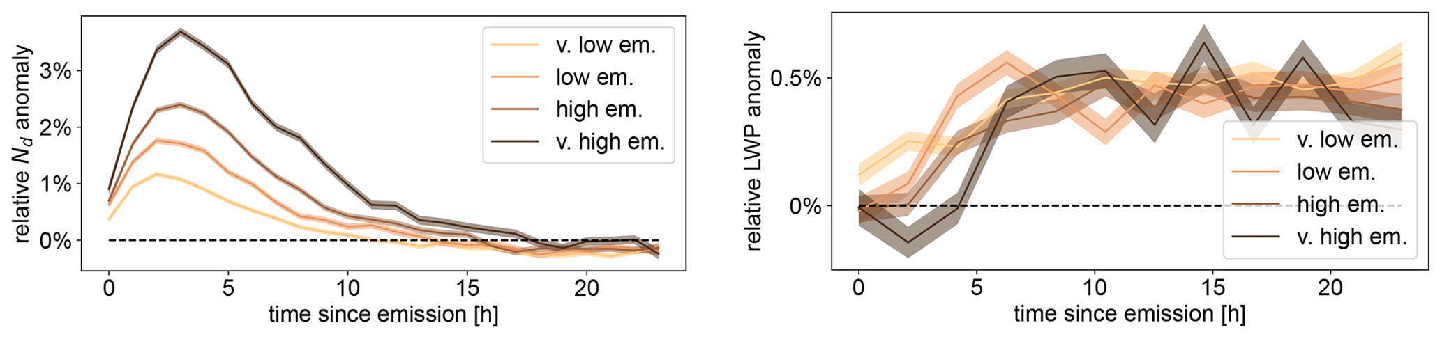
Figure 1 Cloud property responses to ship emissions over time, by emission quartiles. The four equally populated emission bins are labeled very low to very high. These data are from averaging all the data in track that fall into a time and emission bin and dividing them by the average of all the out-of-track data in the same time and emission bin.

Combining the emission and satellite data, we can establish the relationship between emissions and cloud property changes. Figure 1 shows the in-track enhancements of N_d and LWP over the time since emission. The signal shows a maximum around 2 to 4 h after emission and then a slow decline falling to 0 around 15 h. A number of processes are likely responsible for the decline back to 0: the mixing of the track with surrounding air, the onset of precipitation, and the more uncertain location of the retrieved position with longer advection times. The emission amount controls the response in N_d, with the enhancements being larger the larger the emissions are. The same is not true for the LWP response, which seems insensitive to the emissions amount. For all emissions quartiles, the response increases from 0 and reaches a stable state after around 5 h. The level to which it increases is the same for the all quartiles.

3 IMO regulation change

In 2020, the International Maritime Organization (IMO) introduced strict limits on shipping fuel sulfur content, limiting it from 3.5 % to 0.5 % by mass. In some regions, such as off the North American coast and in the North Sea, more stringent limits of 0.1 % have been in place since 2015. However, these areas are small compared to our study region, so the 2020 emission change presents a valuable opportunity to study the effect of low shipping emissions on clouds. Furthermore, compared to other studies on emissions regulation, such as those by Gryspeerdt et al. (2019b) or Watson-Parris et al. (2022), we do not rely on the emissions causing a ship track visible to the eye. Recently, Diamond (2023) has shown the impacts of these changes independently of ship tracks in a shipping corridor in the southeast Atlantic, with a complementary approach to this study.

Figure 2 shows the change in SO_x emissions between 2014 (pre-IMO regulation change) and 2021. Fuel sulfur content was reduced by 80 % after the regulation, and this is reflected in N_d: while N_d enhancement reaches more than 2 % before, it stays well below 1 % after 2020. However, LWP adjustments are of the same magnitude in both cases. This is very similar to the responses by emission quartiles shown in Fig. 1.

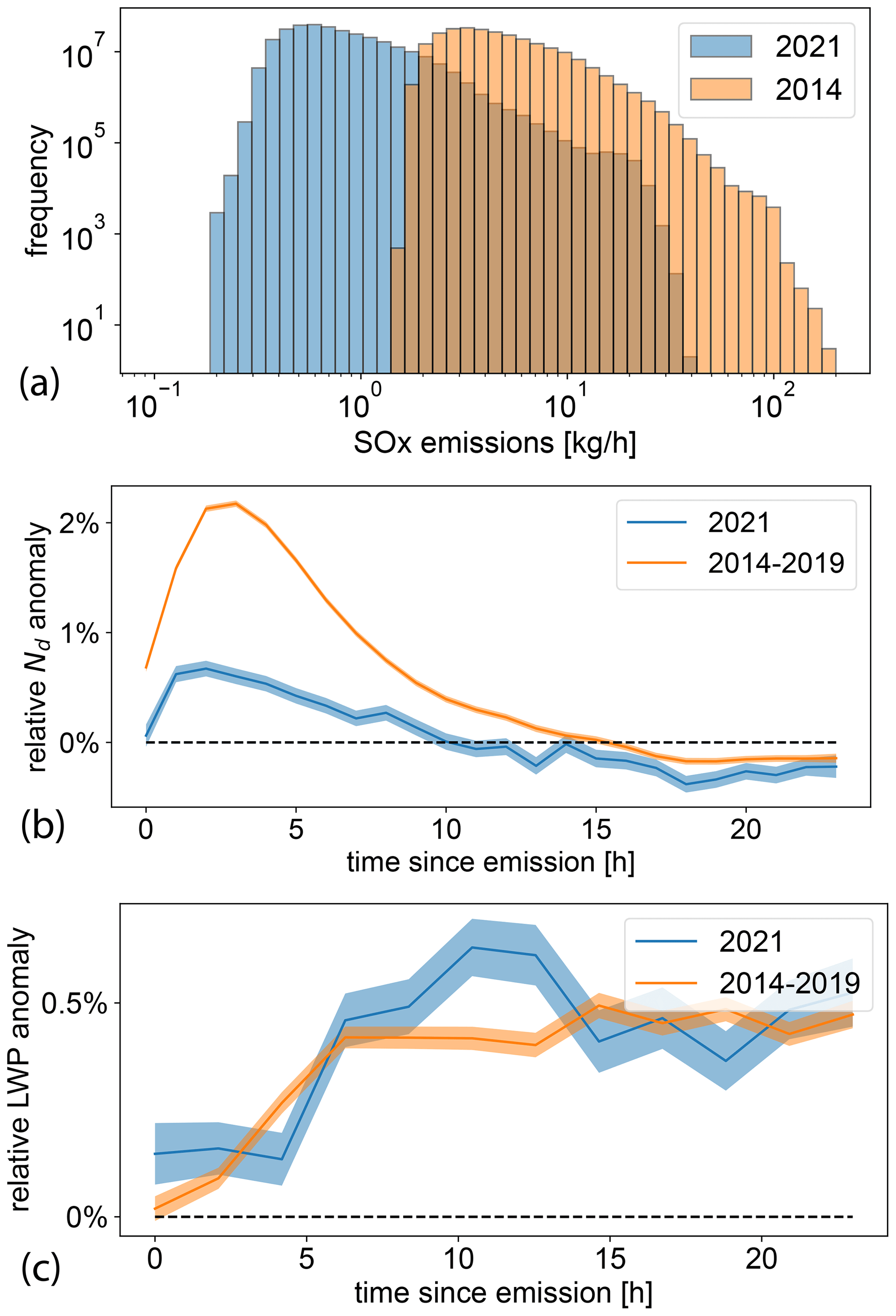
Figure 2 Cloud property responses to IMO fuel sulfur regulation in 2020. Shown in panel (a) is a histogram of sulfur emissions of ships in the study region from the STEAM model, comparing 2014 and 2021. Panels (b) and (c) show the responses of cloud properties N_d and LWP, each time comparing the 6 years before with the year after 2020, when the fuel sulfur content decrease was mandated by the IMO.

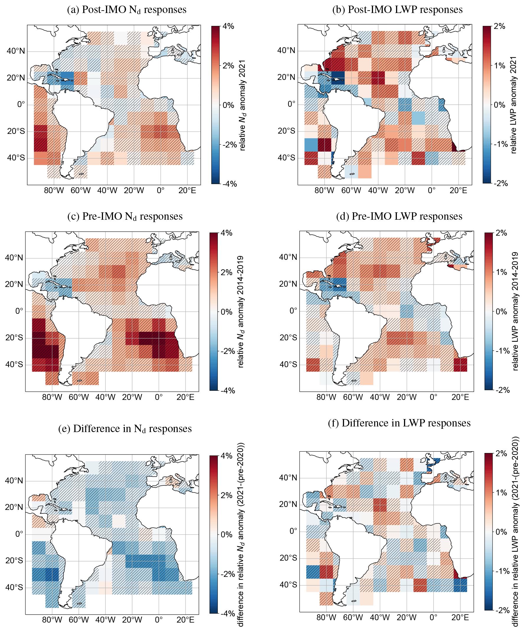
Figure 3 Comparison of regional patterns of N_d and LWP responses before and after sulfur emissions regulation. Heatmaps show the responses in N_d and LWP averaged over 10 h after emissions for N_d and 24 h for LWP. Panels (a) and (b) show the post-regulation responses, panels (c) and (d) the pre-regulation responses, and panels (e) and (f) the differences. Note that the color bar ranges are different for N_d and LWP. Hatching in (a)–(d) indicates statistically significant differences (p < 0.1 in a two tailed Student's t test) from the null experiment (see Methods). In (e) and (f) we test for significant differences between the pre- and post-IMO anomalies. The bottom row has too little ship traffic to collect data.

Figure 3 shows the pre- and post-2020 responses over space in the study region. Figure 3c and d are for 2014 to 2019 as in Manshausen et al. (2022a), whereas Fig. 3a and b are for 2021, and Fig. 3e and f show difference plots. The stratocumulus regions of the southeast Pacific and Atlantic above the cold waters of eastern boundary upwelling regions are those with the strongest N_d anomalies in Fig. 3a and c. The most positive LWP response is in the Atlantic trade cumulus. As with the time-resolved signal in Fig. 2, the response in N_d is different before and after 2020, with the difference plot in Fig. 3e showing decreases in N_d anomaly almost everywhere. These are most pronounced where the N_d anomaly was large before. The LWP response, again, does not seem to change systematically after 2020, with the difference plot in Fig. 3f showing no spatially coherent changes.

4 Dependence on drizzle conditions

If the enhancement in LWP is due to drizzle suppression, then it can be expected to depend on the background droplet radius, as shown by Toll et al. (2017). They use a threshold of droplet effective radius of 15 µm. Above 15 µm we expect the presence of drizzle, increased gravitational settling, and subsequent LWP loss through precipitation. This is the regime where additional aerosol can decrease droplet radii to suppress precipitation and maintain high LWP. Sorting the data by emission quartiles and then into droplet radii below or above 15 µm, we obtain the LWP evolutions of Fig. 4. As hypothesized, they do not show clear enhancements in the no-drizzle case. In the drizzling case however, LWP is enhanced in the track. This supports the mechanism of drizzle suppression for LWP increases.

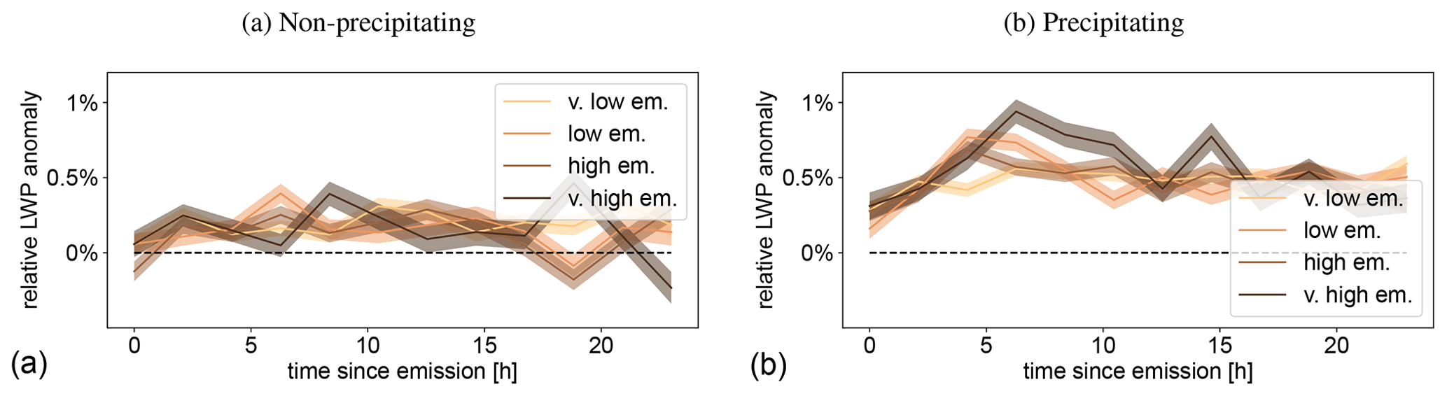
Figure 4 LWP only strongly increases in rainy conditions. LWP responses to ship emissions over time, by emission quartiles. Panel (a) shows non-rainy conditions, with droplet radii smaller than 15 µm; panel (b) shows rainy conditions, with radii greater than 15 µm.

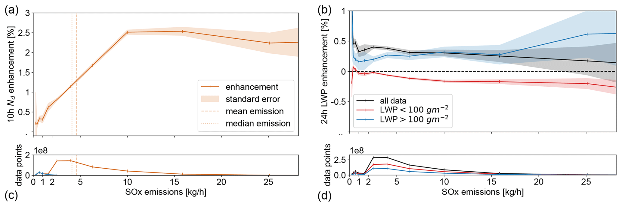
Figure 5 Cloud property responses to ship emission amount. Shown in panel (a) are the N_d response over the first 10 h since emission as a function of emission amount. Inset in the bottom is the number of data points at the given emission amount. Shown in panel (b) in a similar way are the LWP response, for all data as well as stratified by LWP conditions, and the number of points at the bottom.

We can resolve the emission dependence of N_d and LWP, when we do not also stratify by time since emission. Figure 5 shows the emission dependence of N_d and LWP. For N_d, we give the enhancement averaged over the first 10 h after emission, as this gives a stronger signal (compare time-resolved plots like Fig. 1). In the bottom plots we show the number of data points corresponding to a bin of SO_x emissions. The small, blue low-emission peak represents the 2021 data and the larger, orange one the data between 2014 and 2019. Note that in the top panels the orange line includes both 2021 and 2014–2019 data. The response of N_d to emissions is roughly linear over a large range of emissions, well above and below the pre-2020 mean. The response saturates for very high emissions past 10 kg h⁻¹, and it may show nonlinear behavior for very low emissions, cases which are somewhat more uncertain due to the lower number of data points.

Figure 5 also shows the emission dependence of LWP enhancements, for all data and for the subsets where LWP is above or below 100 g m⁻². Results by Suzuki et al. (2015) suggest that 100 g m⁻² of LWP separates higher LWP drizzling and raining from lower LWP non-precipitating clouds. In a similar way as for the stratification by effective radii in Fig. 4, the figure shows LWP increases in the precipitating case. These increases depend on emission but far less than those of N_d. Similarly, in the non-precipitating case, there are LWP reductions that become more important with increasing emissions.

The all-data curve is almost independent of emissions, consistent with the results from the previous sections on quartiles and IMO regulation. For low-emission cases the “all-data” category is even above the high-LWP case. This can be explained because counterintuitively, the all-data category is not exactly the combination of the other two subsets. To avoid regression to the mean biases, we require both the in- and out-of-track data to fulfill the same conditions (see Methods). This means that the all-data category includes those cases where the out-of-track LWP is lower and the in-track LWP higher than 100 g m⁻², not present in either subset. The results show that the LWP response is pronounced even in the lowest observed emission bins.

5 Free-tropospheric relative humidity

Humidity above the cloud is correlated with the cloud property anomalies. Background rainy conditions are necessary for LWP enhancements through precipitation suppression, while LWP reductions are due to cloud top drying. This hinges on the entrainment of dry air, and we therefore expect the relative humidity in the free troposphere to play a role in the overall cloud response to aerosol. For instance, Glassmeier et al. (2021, their Supplement) showed negative LWP adjustments in large eddy simulations at a free-tropospheric water vapor mixing ratio of less than 2.8 g kg⁻¹. Figure 6 shows the enhancements as a function of relative humidity at 700 mbar (RH700, ​​​​​​​a proxy for the – pressure-variable – above-cloud relative humidity). There is a clear covariation of the two, as shown in Fig. 6a and b, where we stratify the N_d and LWP enhancements over time into four RH700 quantiles. The drier the air above the cloud, the stronger the droplet number enhancement. The LWP enhancements behave the opposite way and grow strongest for the most humid quartile. Looking at the enhancements over RH700 bins in Fig. 6c and d we see a large regional difference in N_d, with the stratocumulus showing the largest increase. A difference in cloud regimes may help to explain the change in N_d responses as a function of RH700. In LWP, the stratocumulus behaves similarly to the Azores region, with LWP enhancements small or negative at low humidities and large at high humidities. While this is consistent with precipitation suppression and evaporation enhancement mechanisms, it is unclear what part of the covariability is causal. For instance, RH700 may be correlated to other cloud-controlling factors such as air mass history, aerosol loading, or updraft speeds, which will also influence adjustments to aerosol perturbations.

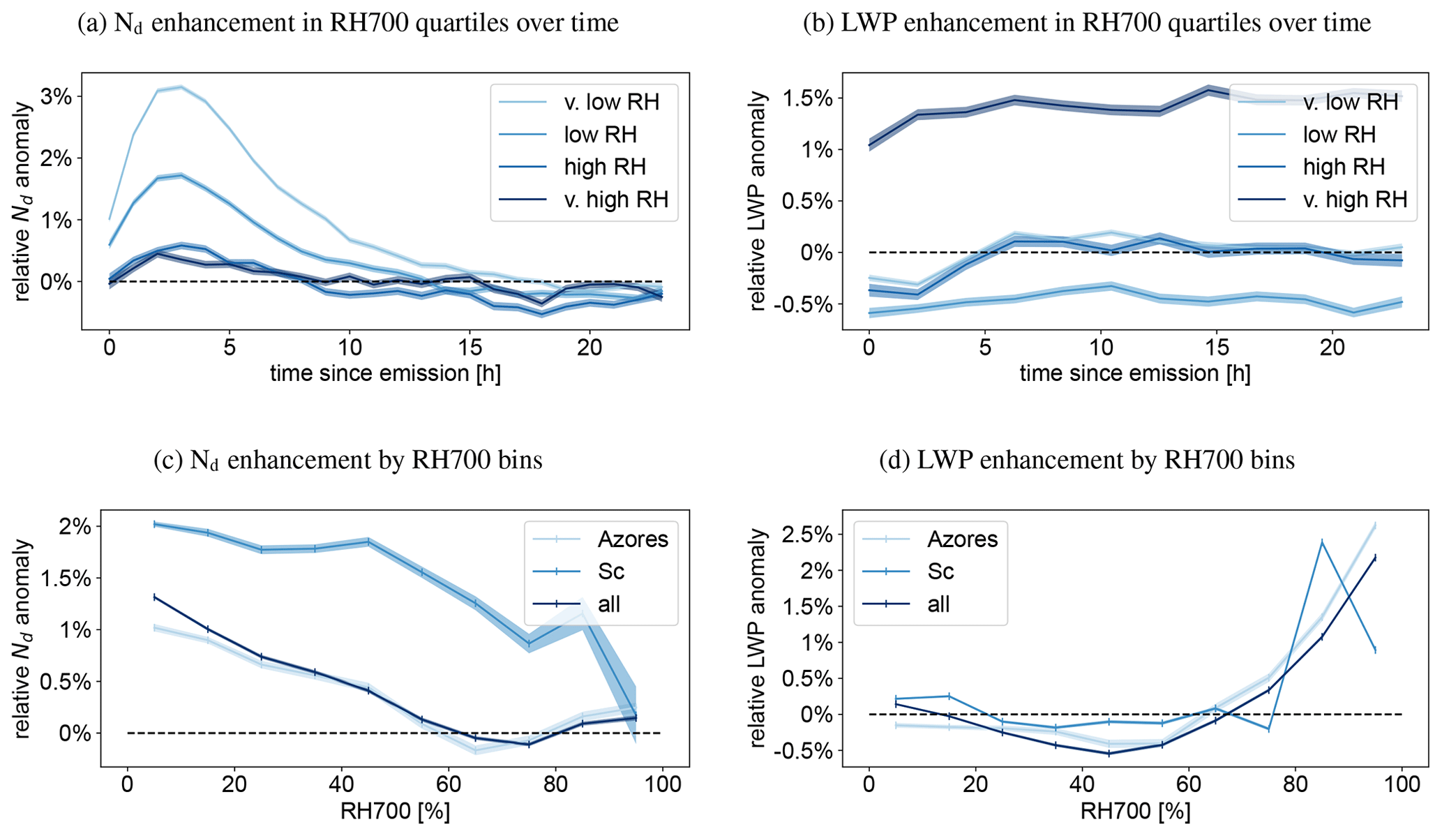
Figure 6 The effect of free-tropospheric relative humidity (at 700 mbar, RH700) on N_d and LWP anomalies. Panels (a) and (b) show the hourly anomalies by quartiles and panels (c) and (d) the averages over time and instead stratified by region (around the Azores and in the Namibian and Chilean stratocumulus, Sc).

6 Discussion and conclusion

We have shown the dependence of cloud properties on aerosol concentrations from shipping pollution using information on ship positions and modeled emissions together with reanalysis winds and satellite retrievals of cloud properties. Specifically, we found a strong dependence of N_d enhancements on emission amounts, with more emissions leading to larger N_d anomalies in tracks. Meanwhile, LWP increases of about the same magnitude are found to occur across all different emission levels.

This is also well supported by the changes from the pre- to post-2020 data, corresponding to an 80 % reduction in sulfur emissions. The corresponding change in N_d anomalies in tracks, much lower in 2021, confirms the changes observed between quartiles of emissions from the STEAM2 model. Similarly, LWP anomalies are largely unchanged before and after 2020 as well as between quartiles of STEAM2 emissions, lending credibility to the model. Having only 1 year of data for the post-IMO regulation period means that there are not as many data as for the pre-IMO regulation data. However, even a single year of ship track data produces O(10⁵) tracks, and results are significant with respect to standard errors. Using a single year can potentially signify different climatological conditions, with different cloud properties in 2021. However, as we are only presenting departures from background states, results would only be different if susceptibility to aerosol changed. This effect is likely small but hard to rule out or quantify without clear knowledge of the cloud-controlling factors, which we are currently investigating. There will also be a change in signal stemming from the cleaner background conditions in 2021, where the aerosol burden in shipping corridors is reduced as a cause of the lower SO_x emissions of the individual ships. We find an average out-of-track N_d of 65.9 cm⁻³ pre-2020 compared to 64.8 cm⁻³ post-2020, a difference that is significant with respect to the standard error of the mean but likely too small to change the “average cloud” sensitivity to aerosol perturbations. This may be different in shipping corridors, which will have experienced a larger decrease because of the high concentration of shipping.

Furthermore, we showed that the LWP enhancements preferentially occur in the drizzling regime where effective radii of cloud droplets are larger than 15 µm and LWP values above 100 g m⁻², consistent with drizzle suppression. In the non-drizzling regime we find no decreases in LWP, expected due to enhanced evaporation at the cloud top, contrary to several studies of visible tracks (Segrin et al., 2007; Christensen and Stephens, 2011; Chen et al., 2012). However, no decreases were observed in our previous study including invisible tracks (Manshausen et al., 2022a) nor in the ship tracks shown by Gryspeerdt et al. (2019a, their Fig. 6). We find that above-cloud relative humidity covaries with LWP adjustments (Fig. 6) and that there are negative adjustments in drier conditions. The emission dependence of increases and decreases in LWP in different regimes may compensate for this, offering a possible lead to explain the weak overall dependence of LWP anomalies on emission amounts. This dependence on environmental conditions is consistent with the findings of Toll et al. (2017). While Gryspeerdt et al. (2019b) find a similar independence of emissions for LWP enhancements, they find LWP enhancements only in low-LWP environments. However, their data are only representative of visible tracks in the stratocumulus cloud regime, while our methodology includes all polluted clouds and all cloud regimes that occur in the study region, in particular trade cumulus.

The weak dependence of LWP enhancements on emission amount is more puzzling because we expect the LWP enhancement to be caused by the previous N_d enhancement, which itself is much more dependent on emissions. A possible explanation for this is a nonlinear or threshold behavior, where even the small enhancement in N_d at low emissions is enough to shut down precipitation. It is possible that we do not have enough very low emission data to observe the case where the N_d response is too small to suppress precipitation. If this threshold behavior is confirmed, it has important implications for calculations of aerosol forcing, which are currently performed using power law relations between the aerosol amount, N_d, and LWP (Bellouin et al., 2020).

This can be compared to the different ways autoconversion, the process that converts cloud droplets to drizzle, is parameterized in global climate models. The threshold behavior of the initiation of autoconversion on cloud liquid-water content has long been known (Kessler, 1969). In modeling, Suzuki et al. (2013) evaluate different thresholds for drizzle formation in autoconversion schemes using radar and MODIS observations. They find that the models which best match the satellite observations are the ones that use a higher threshold for drizzle formation. This means allowing drizzle formation only at effective radii larger than the threshold value. The threshold may not be just a tuning parameter but rather represent a real, nonlinear physical process. However, simply changing autoconversion rates alone may not achieve the desired N_d–LWP relationship (Christensen et al., 2023).

We cannot exclude alternate hypotheses for the observed emission independence of LWP enhancements. For example, Wang et al. (2011) show that in LESs of ship tracks, dynamic effects can lead to decreases in cloud cover in the out-of-track region. If this occurred in the cases we observe, we might be seeing a negative adjustment of LWP out of track rather than a positive one in track. However, our out-of-track retrievals are further away than the dark tracks observed by Wang et al. (2011), which are centered around 15 km from the middle of track compared to the distance of 30 km for our out-of-track retrievals. Furthermore, dynamic responses are also linked to aerosol amounts and therefore should disappear at low emissions like any microphysical responses. Direct injection of water vapor without aerosol (from nuclear-powered ships) showed no cloud responses in the Monterey Area Ship Track (MAST) experiment (Durkee et al., 2000) and therefore seems unlikely to play a role.

Future work will help to elucidate these questions by analyzing cloud perturbations with higher spatial resolution across track, i.e., not only using in-track and out-of-track data but retrieving data at multiple distances from the central estimate of emission locations. This should allow us to discern an in-track increase from an out-of-track decrease in LWP. Similarly, we want to add an analysis of cloud fraction, as quantified by successful retrievals of cloud properties in the pixels across track. The pixel-level retrievals are important, as cloud fraction measures depend on the scale on which they are defined, which makes this analysis more challenging. It may be important because cloud fraction responses have been claimed to be as important as N_d enhancements to the radiative effect of aerosol emissions (Rosenfeld et al., 2019).

Appendix A: Methods

A1 Scope

Geographically, we study the larger part of the Atlantic between (−50^∘ S, 50^∘ N) and (−90^∘ W, 20^∘ E) as well as the stratocumulus (Sc) deck in the southeast Pacific off the Chilean coast. The size of the region is limited by computational cost, and we choose to place it so it covers two Sc regions. Data are for the years 2014–2019 as well as 2021 (chosen to compare the pre- and post-IMO regulation cases).

A2 Retrieval at polluted cloud locations

We find ship-polluted clouds in satellite data without relying on a change in cloud droplet effective radius or on the tracks being visible to the eye. For this, we rely on ship positions from the Automatic Identification System (AIS) system. As the AIS data themselves are proprietary, we reconstruct ship tracks from hourly emission grids provided by the Finnish Meteorological Institute. These are heatmaps at 0.005^∘ spatial resolution. Ship position points are found using the trackpy library (Allan et al., 2019). These positions, interpolated to 5 min intervals, are then used as input to the HYSPLIT model (Stein et al., 2015). The model uses ERA-5 reanalysis data (which were converted into Air Resources Laboratory (ARL) format) together with the initial position and an assumed emission height of 20 m to simulate the location of the advected emissions up to 24 h after emission (this is on the lower end of the emission height of most ships but produces the best-matched tracks in visual inspection of test days with visible tracks). Out-of-track retrievals are taken by using the shape of the advected emissions track but 30 km to either side of the track. This is done by calculating the “direction” of a track, taken as the vector from start to end, then calculating the orthogonal vector, and then displacing the track by 30 km in the orthogonal vector's direction. For a given overpass of the Aqua or Terra satellites, which carry the Moderate Resolution Imaging Spectroradiometer (MODIS) (Platnick et al., 2003), the positions of the emissions at this time is selected and collocated to the MODIS Level-2 cloud product MOD/MYD 06, collection 6.1. N_d is obtained following Quaas et al. (2006) from retrievals of cloud optical thickness and effective radius (see also the derivation to Eq. 11 in Grosvenor et al., 2018). Compared to hand-logged tracks, the retrieval locations are less certain, owing to uncertainty in the reanalysis wind data used to advect the emissions. This means that overall the enhancements are smaller compared to natural variability; i.e., there is a lower signal-to-noise ratio than in ship track studies. This problem is tackled with a large number of data as well as careful sampling to avoid introducing any biases (see below for conditioning on retrieved properties).

A3 Input for modeling ship emissions

The Ship Traffic Emission Assessment Model of the Finnish Meteorological Institute (STEAM) uses the following datasets as input:

• a.

  Vessel activity. This consists of global AIS transponder messages, which include data both from terrestrial and satellite AIS networks. Global vessel activity datasets are provided by commercial operators and restricted to Finnish Meteorological Institute (FMI) research purposes. These are currently provided by Orbcomm Ltd.

• b.

  Global fleet description. These data include technical features of all the ships in the global fleet and are provided by a commercial operator. Required data include physical dimensions, machinery, propulsion system details, power generation and transmission features, capacity description, and installation of emission abatement techniques (e.g., exhaust gas cleaning systems). In this case, data from IHS Markit and IMO GISIS are used.

• c.

  Polygon descriptions of special areas. These include, for example, emission control areas (ECAs) for air emissions. These input datasets define, for each vessel, its capabilities of using various fuels during the modeling runs. These are defined by engine properties, operation area, and time stamp (for entry into force of regulation). Environmental conditions such as sea current and surface wind speed and direction can in principle be added to the model. Here, they are not considered because they would slow the computation down so that the resolution would need to be lowered.

A4 Emissions model

We are giving a high-level description of the STEAM calculation process. For the details of the calculation process, see Jalkanen et al. (2012) and Johansson et al. (2017). In STEAM, vessel resistance is determined by the following components.

$$\begin{array}{}\text{(A1)}& R_{\mathrm{total}}=R_{\mathrm{residual}}+R_{\mathrm{friction}}+R_{\mathrm{fouling}}\end{array}$$

Once R_total is known, the necessary engine power P is determined from

$$\begin{array}{}\text{(A2)}& P={\displaystyle \frac{R_{\mathrm{total}}{v}_{\mathrm{inst}}}{q}},\end{array}$$

in which q is the quasi-propulsive constant, which includes the propulsive losses of power transmission and propeller efficiency. The calculation is described by Watson (2002) and includes contributions from propeller rotation speed and vessel length. Additional components of performance prediction include the effect of waves and sea currents, but these are regarded as modifications of vessel speed (knots) not resistance (kilonewtons). The individual resistance components of R_tot are modeled using the following methods: R_residual comes from the Hollenbach resistance prediction (Jalkanen et al., 2012), which is a parameterized model based on resistance tests of 433 vessels and considers, e.g., vessel hull shape, bulbous bows, and different resistance components. R_friction and R_fouling uses the ITTC method to determine hull friction and fouling, respectively (ITTC, 2017).

A5 Conditioning on background effective radii and LWP

The data of advected emissions tracks are noisy. Therefore, subsetting the dataset following any kind of criterion needs to be done very carefully. Consider the case where we would like to look at precipitating conditions as indicated by effective radii. Naively, we would subset the data such that in our subset the out-of-track regions have r_eff>15 µm. However, given noisy observations (random errors from imperfect collocation), this would introduce a bias. If there were no effect of the ship but the data were following the same distribution in the track and the out-of-track data, “cutting off” the lower effective radius part of the out-of-track distribution would lead to different means of the track and the out-of-track data. Instead, we have no choice but to require both the out-of-track and the track data to have r_eff>15 µm. Stratifying them this way for the below and above threshold cases, however, excludes all those cases where the track and background are on different sides of the threshold – arguably the situation we would like to observe, where precipitation that is going on outside of the track is shut down within. This is mitigated by the large size of the retrieval area (20 km across), where ship tracks should be smaller than this. Then, even if in the track-effective radii are reduced, the mean of the retrieval may still be above the threshold in a precipitating regime.

A6 Null experiments

To validate our method and to assure that increases in N_d and LWP are indeed linked to the shipping (rather than the result of a bias), we also perform a null experiment. This consists in retrieving data at the locations of the advected tracks but in the satellite data of the day before the ships pass through. In the collocation of advected emissions with satellite data described above, we select the emissions that were emitted up to 24 h before each satellite overpass, find their positions at the overpass time, and collocate them. If we change this to use the emissions that occur in the 24 h after the overpass and advect them until the overpass time on the next day, this gives us a sampling strategy that will show the same kind of retrieval geometry but without the pollution from individual ships. Here, we expect no signal, and indeed, in Fig. A1, treating the data otherwise in the same way as in the experiment, i.e., stratifying them by emission quartiles and effective radii, we see no strong response and possibly even a small decrease. This may be due to natural variability or the effects of other ships preferentially taking the same routes (shipping corridors), and this signal should also be present in the actual observations.

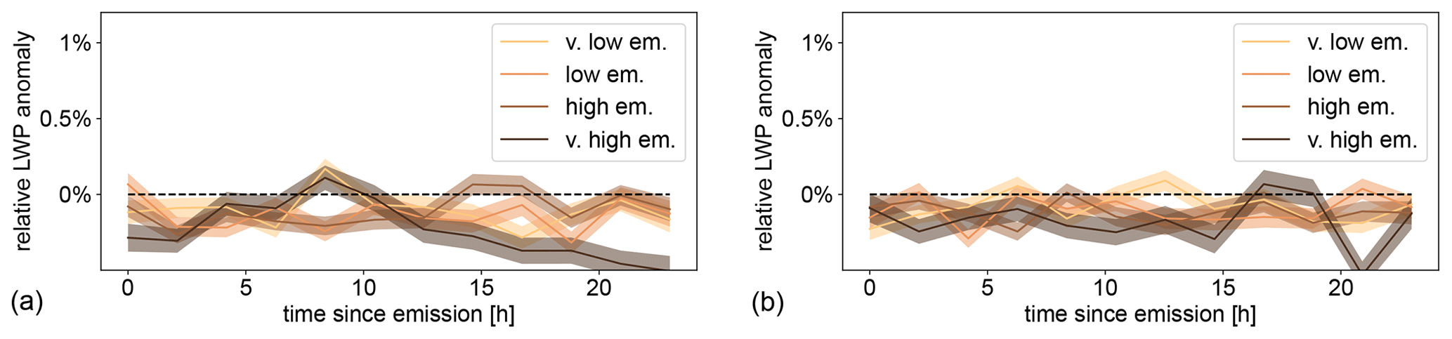
Figure A1 No significant LWP response in a control experiment. Here, retrievals are done with the same geometry as before but using the positions of ships that have not yet passed through the retrieval region. Panel (a) shows non-rainy conditions, with droplet radii smaller than 15 µm; panel (b) shows rainy conditions, with radii greater than 15 µm.