the Creative Commons Attribution 4.0 License.
the Creative Commons Attribution 4.0 License.
 | 12 Sep 2023
A multimodel evaluation of the potential impact of shipping on particle species in the Mediterranean Sea
Matthias Karl
Volker Matthias
Sonia Oppo
Richard Kranenburg
Jeroen Kuenen
Sara Jutterström
Jana Moldanova
Elisa Majamäki
Jukka-Pekka Jalkanen
Shipping contributes significantly to air pollutant emissions and atmospheric particulate matter (PM) concentrations. At the same time, worldwide maritime transport volumes are expected to continue to rise in the future. The Mediterranean Sea is a major short-sea shipping route within Europe and is the main shipping route between Europe and East Asia. As a result, it is a heavily trafficked shipping area, and air quality monitoring stations in numerous cities along the Mediterranean coast have detected high levels of air pollutants originating from shipping emissions.
The current study is a part of the EU Horizon 2020 project SCIPPER (Shipping Contributions to Inland Pollution – Push for the Enforcement of Regulations), which intends to investigate how existing restrictions on shipping-related emissions to the atmosphere ensure compliance with legislation. To demonstrate the impact of ships on relatively large scales, the potential shipping impacts on various air pollutants can be simulated with chemical transport models.
To determine the formation, transport, chemical transformation, and fate of particulate matter < 2.5 µm (PM2.5) in the Mediterranean Sea in 2015, five different regional chemical transport models (CAMx – Comprehensive Air Quality Model with Extensions, CHIMERE, CMAQ – Community Multiscale Air Quality model, EMEP – European Monitoring and Evaluation Programme model, and LOTOS-EUROS) were applied. Furthermore, PM2.5 precursors (ammonia (NH3), sulfur dioxide (SO2), nitric acid (HNO3)) and inorganic particle species (sulfate (SO), ammonia (NH), nitrate (NO)) were studied, as they are important for explaining differences among the models. STEAM (see “List of abbreviations” in Appendix A) version 3.3.0 was used to compute shipping emissions, and the CAMS-REG version 2.2.1 dataset was used to calculate land-based emissions for an area encompassing the Mediterranean Sea at a resolution of 12 × 12 km2 (or 0.1∘ × 0.1∘). For additional input, like meteorological fields and boundary conditions, all models utilized their regular configuration. The zero-out approach was used to quantify the potential impact of ship emissions on PM2.5 concentrations. The model results were compared with observed background data from monitoring sites.
Four of the five models underestimated the actual measured PM2.5 concentrations. These underestimations are linked to model-specific mechanisms or underpredictions of particle precursors. The potential impact of ships on the PM2.5 concentration is between 15 % and 25 % at the main shipping routes. Regarding particle species, SO is the main contributor to the absolute ship-related PM2.5 and to total PM2.5 concentrations. In the ship-related PM2.5, a higher share of inorganic particle species can be found when compared with the total PM2.5. The seasonal variabilities in particle species show that NO is higher in winter and spring, while the NH concentrations displayed no clear seasonal pattern in any models. In most cases with high concentrations of both NH and NO, lower SO concentrations are simulated. Differences among the simulated particle species distributions might be traced back to the aerosol size distribution and how models distribute emissions between the coarse and fine modes (PM2.5 and PM10). The seasonality of wet deposition follows the seasonality of the precipitation, showing that precipitation predominates wet deposition.
- Article
(3429 KB) - Full-text XML
-
Supplement
(2932 KB) - BibTeX
- EndNote


Exhaust particles emitted from shipping have a large share in total emissions from the transport sector (Corbett and Fischbeck, 1997; Eyring et al., 2005), thereby affecting the chemical composition of the atmosphere as well as the regional air quality. Particularly in coastal areas, maritime transport contributes a considerable fraction to air pollution (Viana et al., 2014).
High particulate matter < 2.5 µm (PM2.5) concentrations can be caused by transported particles, desert dust, or the production of secondary particulate matter (Tomasi and Lupi, 2017). Previous studies have revealed that in Europe the PM2.5 concentration increase caused by shipping emissions is small (Viana et al., 2009; Aksoyoglu et al., 2016). Nevertheless, in the Mediterranean region the relative ship impact on the PM2.5 concentration is large, with a share of 5 % to 20 % of the total PM2.5 concentration (e.g., Aksoyoglu et al., 2016; Nunes et al., 2020). The formation of secondary particulate matter from ship emissions is of particular importance. According to Viana et al. (2009), the secondary contribution of ship emissions is equivalent to double their primary contribution. Secondary particles in the atmosphere form from gaseous precursors, whereas primary particles are directly emitted and evolve within a short time to form secondary particles. To improve the air quality in coastal regions, it is important to identify the pollutant sources and make reliable estimations of their impacts on surrounding PM levels. It has been shown that the majority of secondary particles contributing to local PM in ports come from shipping (Song and Shon, 2014). Furthermore, according to Klimont et al. (2017), the proportion of international shipping's particulate matter primary emissions to global anthropogenic emissions is between 3 % and 4 %, which is comparable to road traffic. Additionally, shipping contributions to total PM2.5 concentrations far from coastlines were found to be responsible for exceedances of the WHO air quality guideline values (Nunes et al., 2020). The annual mean PM2.5 limit value in the EU is 25 µg m−3 (EU DIRECTIVE 2008/50/EC, 2008), whereas the annual mean PM2.5 goal established by the WHO is 5.0 µg m−3 (WHO, 2021). Strong evidence has been found for the relationship between exposure to PM2.5 and the occurrences of certain diseases affecting the lungs, cancer, or type 2 diabetes (Heusinkveld et al., 2016; Chen et al., 2016; Gao and Sang, 2020). According to the WHO, there is no safe level of PM2.5; thus, the gap between the WHO and EU's PM2.5 values is of real concern (Karamfilova, 2022).
The MEPC decided in December 2022 to establish a sulfur emission control area in the Mediterranean Sea by 1 January 2025. In this area, the limit for sulfur in fuel oils used on board ships is 0.10 % (IMO, 2022). The global sulfur cap for marine vessels came into effect in January 2020, which declares that the sulfur content of any fuel oil used from ships must not exceed 0.50 % m m−1, except for ships using “equivalent” compliance mechanisms, such as scrubbers. Calculations show that this policy has led to PM2.5 reductions ranging from 0.5 µg m−3 to more than 2.0 µg m−3 along the major shipping routes in the Mediterranean Sea (Jonson et al., 2020). These relatively strict 2020 regulations are expected to lower the number of PM2.5-related premature deaths by on average 15 % (Viana et al., 2020).
Although the Mediterranean Sea contains one of the busiest shipping routes worldwide, only a few regional-scale chemical transport modeling studies have considered this region. Viana et al. (2014) reviewed studies concerning the impacts of shipping emissions on air quality in European coastal areas, noting that the highest PM2.5 contributions were found in the Mediterranean Sea and North Sea. Aksoyoglu et al. (2016) studied PM2.5 concentrations in the Mediterranean Sea followed by a comparison of two models. Marmer and Langmann (2005) investigated the Mediterranean Sea on a broader scale and without comparing different CTM systems. Nevertheless, other studies have concentrated on smaller domains, such as the Iberian Peninsula (Baldasano et al., 2011; Nunes et al., 2020), the eastern Mediterranean Sea with the Arabian Peninsula (Večeřa et al., 2008; Tadic et al., 2020; Celik et al., 2020; Friedrich et al., 2021), or the urban scale and harbor cities (Schembari et al., 2012; Donateo et al., 2014; Prati et al., 2015). None of these studies, however, analyzed the potential shipping impacts on PM2.5 concentrations together with individual aerosol species on a regional basis while additionally comparing the results of five CTMs.
A wide range of gaseous pollutants, such as sulfur dioxide (SO2) and nitrogen oxide (NOx= NO + NO2), coming from shipping emissions can be precursors for particle formation (Jägerbrand et al., 2019; Karl et al., 2019; Matthias et al., 2010). Sulfur dioxide is released mainly by human activities such as fossil fuel burning, petroleum refining, and metal smelting (Zhong et al., 2020). SO2 is oxidized by dissolved oxidants such as ozone (O3) and hydrogen peroxide (H2O2) in the aqueous phase and by hydroxyl (OH) in the gas phase to generate sulfuric acid (H2SO4) (Seinfeld and Pandis, 2006). H2SO4 and nitric acid (HNO3) react with ammonia (NH3) to form ammonium sulfate ((NH4)2SO4) and NH4NO3 aerosols, with H2SO4 neutralization having preference due to its lower vapor pressure (Hauglustaine et al., 2014).
Nitrogen oxides are primarily removed during the day via the OH radical oxidation reaction to produce (HNO3) (Seinfeld and Pandis, 1998). At night, the main NOx removal method involves interacting with O3 to produce the nitrate (NO3) radical, which may then combine with nitrogen dioxide (NO2) to form dinitrogen pentoxide (N2O5) and may subsequently undergo a heterogeneous reaction with water to produce HNO3. As it is highly soluble, HNO3 disperses quickly in water droplets or is neutralized by reaction with NH3 to produce NH4NO3 aerosols. Increased emissions of NH3 or HNO3 formation and their deposition negatively affect the environment through eutrophication and acidification, thereby contributing to the loss of ecosystem biodiversity (Remke et al., 2009; Kleijn et al., 2009; Krupa, 2003).
Furthermore, the air pollution status should be assessed to investigate the consequences of new legislation.
The current work investigates and analyzes the predictions of five different CTMs for air pollutant dispersion and transformation. The intercomparison was carried out in two parts: part one included the photochemistry and differences among the models regarding NO2 and O3 (Fink et al., 2023). The present study is part two of the model intercomparison and evaluates the same CTM simulations but different air pollutants, namely aerosols. This paper is structured as follows: Sect. 3.1 and 3.2 consider the simulated overall PM2.5 model performance and spatial distribution. In Sect. 3.3, precursors (NH3, HNO3, SO2, and NO2) are investigated as the basis for inorganic particle species. Inorganic aerosol concentration and wet deposition are regarded in Sect. 3.4.
To date, the present study is the first multimodel study designed to compare the potential impacts of shipping on PM2.5 and particle species simulated by five regional-scale CTMs for the Mediterranean Sea.
In this section the models participating in the intercomparison study are briefly described. More detailed information about the standard setup of the models and model internal mechanisms used in the present study can be found in part one of this intercomparison study (Fink et al., 2023), which focuses on nitrogen oxides and ozone.
2.1 Models
In this study, five different regional-scale CTM systems run by four institutions participated: CAMx and CHIMERE run by AtmoSud, CMAQ run by Helmholtz-Zentrum Hereon, EMEP run by the IVL Swedish Environmental Research Institute, and LOTOS-EUROS run by the TNO Netherlands Organization for Applied Scientific Research. In order to produce comparable results with respect to the impact of shipping emissions on PM2.5 concentrations, the models were set up in a similar way. The same shipping emissions data from STEAM (version 3.3.0.; Jalkanen et al., 2009, 2012; Johansson et al., 2013, 2017) were used for all CTMs. Land-based emissions (CAMS-REG, v2.0), grid projection (WGS84_longlat), domain (Mediterranean Sea), grid resolution (0.1∘ × 0.1∘, 12 × 12 km), and the modeled year (2015) were also consistent (Table 1). The CTM systems were applied in their standard setup for other input data; i.e., the meteorological input data and the boundary and initial conditions differed.
The model domains covered the largest part of the Mediterranean Sea, with a spatial extent ranging in latitude from 33.8 to 44.95∘ and in longitude from −0.95 to 29.95∘ (Appendix A). The appointed grid cell size was 12 × 12 km2 interpolated on a 0.1∘ × 0.1∘ grid nested in a 36 × 36 km2 grid (except EMEP).
A reference run for present air quality conditions was performed using all models, including all emissions (base case). Furthermore, all models ran once without shipping emissions (no-ship case). The difference between the estimates with all emissions and the calculations without shipping emissions was then used to calculate the potential impact of ships on pollutant concentrations (zero-out method).
From the results of all models, the annual averaged ensemble mean was calculated based on the daily files. The model run outputs all contained PM2.5 in micrograms per cubic meter (µg m−3) at a daily resolution on a 2-D grid from the lowest layer and provides this as a netcdf file following CF conventions. Concentrations in the lowest layer close to ground were used for the intercomparison. The CTM systems calculated PM2.5 concentrations in different ways depending on the major physical and chemical mechanisms implemented. Table 1 summarizes the model setups.
The models used in the intercomparison are listed as follows:
-
CAMx v6.50 (Ramboll Environment and Health, 2020),
-
CHIMERE 2017r4 (Menut et al., 2013),
-
CMAQ v5.2 (Byun and Schere, 2006; Appel et al., 2017),
-
EMEP MSC-W (Simpson et al., 2012, 2020), and
-
LOTOS-EUROS v2.0 (Manders et al., 2017).
Detailed descriptions of the models used can be found in the first part of the intercomparison study (Fink et al., 2023).
Table 1Main model parameters and input data for the five chemical transport models.
2.1.1 Aerosol modules
CAMx includes algorithms for inorganic aqueous chemistry (RADM–AQ), inorganic gas–aerosol partitioning (ISORROPIA), and two organic gas–aerosol partitioning and oxidation approaches (VBS or SOAP). Using gas-phase processes, these approaches produce sulfate, nitrate, and condensable organic gases. The hybrid 1.5-D VBS is applied to provide a unified framework for gas–aerosol partitioning and the chemical aging of both primary and secondary atmospheric organic aerosols (Ramboll Environment and Health, 2020). One crucial assumption in PSAT is that PM is allocated to the primary precursor for each type of particulate matter (i.e., PSO4 is apportioned to SOx emissions, PNO3 is apportioned to NOx emissions, and PNH4 is apportioned to NH3 emissions).
A detailed description of CHIMERE's inorganic and organic modules can be found in Menut et al. (2013). CHIMERE's sectional aerosol module includes emitted TPPM and secondary species such as nitrate, sulfate, ammonium, and SOAs. Natural dust and sea salt aerosols can also be produced as passive tracers or interactive species in equilibrium with other ions. Organic matter and elemental carbon can be speciated if an inventory of their emissions is supplied. The utilized models include the aqueous, gaseous, and particulate phases of ammonia, ammonium, nitrate, and sulfate. For instance, in accordance with the ISORROPIA thermodynamic equilibrium model, the model species pNH3 represents an equivalent ammonium in the particulate phase as the sum of the NH ion, NH3 liquid, NH4NO3 solid, and other salts (Nenes et al., 1998).
CMAQ represents aerosol formation and growth using three log-normal-distributed modes: the Aitken and accumulation modes are generally less than 2.5 µm in diameter, while the coarse mode contains significant amounts of mass above 2.5 µm. PM2.5 and PM10 can be obtained from the model-predicted mass concentration and size distribution information.
The CMAQ aerosol scheme AERO6 was employed; this scheme expands the chemical speciation of PM by the species Al, Ca, Fe, Si, Ti, Mg, K, and Mn. Sulfuric acid (H2SO4), nitric acid (HNO3), hydrochloric acid (HCl), and ammonia (NH3) gas-phase–aerosol partition equilibria are solved by the ISORROPIA II mechanism (Fountoukis and Nenes, 2007; Nenes et al., 1998). Contained within this scheme is the formation of SOA from isoprene, terpenes, benzene, toluene, xylene, and alkanes (Carlton et al., 2010; Pye and Pouliot, 2012). CMAQ allows for dynamic mass transfer of semivolatile inorganic gases to coarse-mode particles, which facilitates the replacement of chloride by NO in sea salt aerosols (Foley et al., 2010).
The EMEP MSC-W model version used was rv4.34 with chemical mechanism EmChem 19a (Simpson et al., 2012; Simpson et al., 2020). The mechanism builds on surrogate VOC species (as in Simpson et al., 2012, but extended with benzene and toluene) and has 171 gas-phase and heterogeneous reactions. The model always assumes equilibrium between the gas and aerosol phases using the MARS equilibrium module of Binkowski and Shankar (1995). For SOAs a VBS approach is used (Robinson et al., 2007; Donahue et al., 2009; Bergström et al., 2012). The semivolatile ASOA and BSOA species are considered to oxidize (age) in the atmosphere via OH reactions, whereas all POA emissions are treated as nonvolatile to maintain the emission totals of both the PM and the VOC components from the official emission inventories (Simpson et al., 2012). The aerosol module of the EMEP model distinguishes five classes of fine and coarse particles (fine-mode nitrate and ammonium, other fine-mode particles, coarse nitrate, coarse sea salt, and coarse dust); for dry-deposition purposes, these particles are assigned mass median diameters (Dp), geometric standard deviations (σg), and densities (ρp). The aerosol components that are taken into account include sea salt, SO, NO, NH, and anthropogenic main PM. Aerosol water is also considered.
LOTOS-EUROS uses the TNO CBM-IV scheme, which is a modified version of the original CBM-IV scheme (Whitten et al., 1980). N2O5 hydrolysis is described explicitly based on the available (wet) aerosol surface area (Schaap et al., 2004). The aqueous phase and heterogeneous formation of sulfate are described by a simple first-order reaction constant (Schaap et al., 2004; Barbu et al., 2009). Aerosol chemistry is represented using ISORROPIA II (Fountoukis and Nenes, 2007).
2.1.2 Wet-deposition mechanisms
Wet deposition is the predominant removal process for fine particles. The CAMx wet-deposition model uses a scavenging method in which the local concentration change rate inside or under a precipitating cloud is determined by a scavenging coefficient. From the top of the precipitation profile to the surface, wet scavenging is estimated for each layer inside a precipitating grid column. The scavenging coefficients of gases and PM are calculated differently depending on the correlations given by Seinfeld and Pandis (2006) (Ramboll Environment and Health, 2020). The wet-deposition process in CHIMERE follows the scheme proposed by Loosmore and Cederwall (2004). In CMAQ, wet deposition is calculated in cloud chemistry treatments. The resolved cloud model calculates the contribution of each model layer to the precipitation. Based on a normalized profile of precipitating hydrometeors, CMAQ operates a simple algorithm to assign precipitation amounts to individual layers (Foley et al., 2010). The EMEP model's parameterization of wet-deposition processes covers both the in-cloud and the sub-cloud scavenging of gases and particles. The parameterization of wet deposition is described in Berge and Jakobsen (1998). There are two types of wet deposition in LOTOS-EUROS: below-cloud scavenging and in-cloud scavenging. The technique is described in Seinfeld and Pandis (2006), and Banzhaf et al. (2012) served as the foundation for the in-cloud scavenging module.
2.2 Emissions
2.2.1 Land-based emissions
All five models used anthropogenic land-based gridded emissions from the CAMS-REG v2.2 emission inventory for 2015, which is described in Granier et al. (2019) and is essentially a further development of the earlier TNO_MACC inventories (Kuenen et al., 2014). A more recent version, CAMS-REG-v4.2, is described in detail in Kuenen et al. (2022).
For each country, the gridded emission files included GNFR emission sectors for the air pollutants NOx, SO2, NMVOC, NH3, CO, PM10, PM2.5, and CH4. The spatial resolution of the emissions data was ∘ × ∘ in longitude and latitude (i.e., 6 km over central Europe). The CAMS-REG inventory also provides default information in order to apply the emissions in the CTMs. The height distribution of emissions per GNFR sector was prepared according to Bieser et al. (2011). Based on the assignment of PM and NMVOC components at a detailed subsector level, PM and NMVOC speciation profiles are provided for each country, year, and GNFR sector. The temporal distribution of emissions is based on the default temporal variation provided along with the CAMS-REG inventory. The NOx splitting was performed according to Manders-Groot et al. (2016).
2.2.2 Shipping emissions
The shipping emission dataset produced with the STEAM model has a spatial resolution of 12 × 12 km2 and a temporal resolution of 1 h. The STEAM v3.3.0 emissions are divided into two vertical layers (0 to 36 m; 36 to 1000 m) and are provided for mineral ash, carbon monoxide (CO), carbon dioxide (CO2), elemental carbon (EC), NOx, organic carbon (OC), PM2.5, particle number count (PNC), sulfate (SO4), SOx (containing SO2 and SO3), and VOCs. To reduce the number of generated emission maps and the computational resources needed to run the STEAM model, VOC emissions were divided into four categories according to their properties as a function of the engine load. Emission factors for VOCs are based on the average values taken from various publications (Agrawal et al., 2008, 2010; Sippula et al., 2014; Reichle et al., 2015).
All shipping emissions are included in the lowest layer of CAMx. In CAMx, all gridded emissions are at the ground level except punctual and linear emissions. For CHIMERE, 88 % of the emissions below 36 m and all shipping emissions above 36 m were added to the second layer. Only 12 % of the emissions below 36 m were allocated to the model's lowest layer. The STEAM emission dataset, which included stack heights, was used for this procedure. In CMAQ, shipping emissions were split between the two lowest levels; those below 36 m were ascribed to the lowest layer, while those above 36 m were positioned in the second layer. The heights of the lowest and the second layer in CMAQ are 42 m for each. The STEAM emissions were summed from hourly to daily emissions and were attributed to the lowest layer (up to 90 m) in the EMEP simulations. In LOTOS-EUROS, emissions below 36 m were divided into two layers: the first layer was 25 m thick (∼ 70 % of emissions), and the second layer was 30 m thick (∼ 30 % of emissions). Over 36 m, emissions were separated into various height groups: 30 % were between 36 and 90 m, 30 % were between 170 and 90 m, 30 % were between 170 and 310 m, and 10 % were between 310 and 470 m. These emissions were placed in the second or third model layers because of the dynamic second model layer, which follows the meteorological boundary layer. All emissions were placed in this second layer when the meteorological boundary layer was well mixed and vertically extended (higher than 470 m), while some emissions were placed in the third layer when the boundary layer was shallow.
2.3 Observational data, statistical analysis, and analysis of model results
The model findings regarding the total surface PM2.5 concentrations from the five CTM systems were compared with data from the air quality monitoring network obtained from the EEA's download service (https://discomap.eea.europa.eu/map/fme/AirQualityExport.htm, last access: 6 September 2023). The locations of the measurement stations are shown in Fig. A1, and detailed information on the stations can be found in Appendix B.
The stations were chosen based on the following criteria: (i) the station type was “background”; (ii) the station elevation was less than 1000 m; and (iii) the station recorded data for more than one of the following pollutants – NO2, O3, or PM2.5. In the first part of this intercomparison study (Fink et al., 2023), NO2 and O3 were discussed. Since simulating the potential impact of ships was the main focus of this study, stations near the sea were the preferable choice.
The model findings regarding the total surface PM2.5 concentrations from the five CTM systems were compared with existing observations. The RMSE, NMB, and correlation coefficient R were determined for each monitoring station to quantify the model performance, as described in the previous study (Fink et al., 2023).
A categorization scheme for the correlations was established as described in Schober et al. (2018), with weak (0.00–0.39), moderate (0.40–0.69), and strong (0.70–1.00) correlations.
To compare the predicted daily mean concentrations with the measurements recorded at representative sites, time series were employed. In addition, based on hourly data, the yearly mean potential ship impact was determined. Boxplots based on yearly values obtained from hourly data at each station were used to graphically compare the model performances using the R, NMB, and RMSE metrics. Annual mean values based on hourly data were utilized for the intercomparison maps. Based on hourly data, the correlations between models were determined for each grid cell.
3.1 PM2.5 model performance
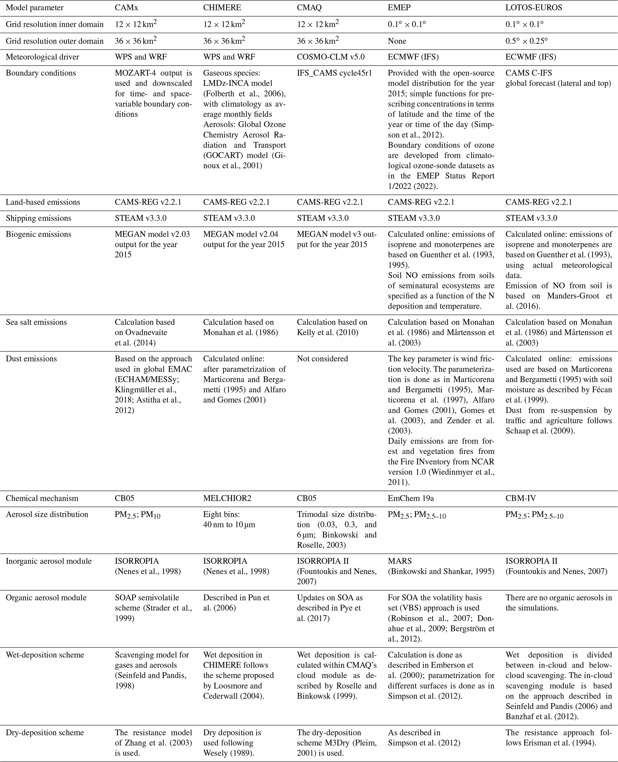
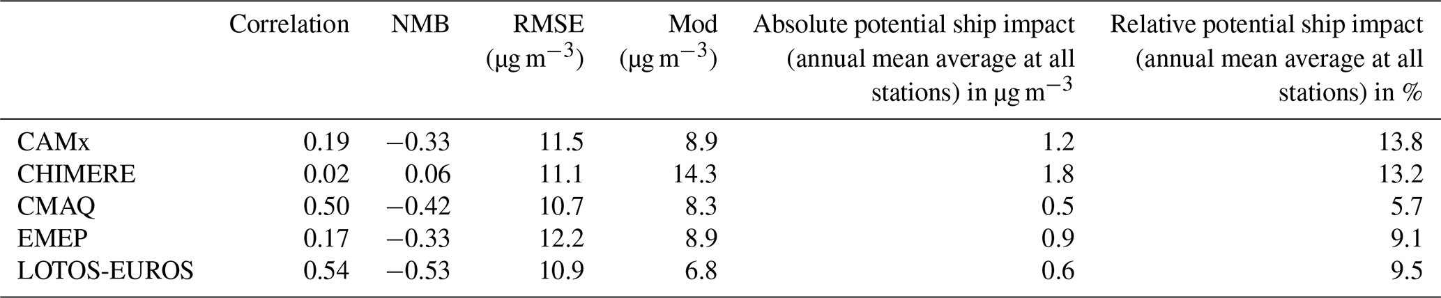
Regarding the model performance, time series can give an overview of the performance throughout the whole year. Figure 1 displays the average values at all 28 measurement stations. CAMx, CMAQ, EMEP, and LOTOS-EUROS underestimate the actual measured data. The largest underestimations are found for CMAQ (NMB = −0.42) and LOTOS-EUROS (NMB = −0.54). Contrary to the other CTM systems, CMAQ does not consider the contribution of dust, which can cause underestimations of PM2.5. However, the correlations between the modeled and measured data are strongest for these models (CMAQ: R= 0.50, LOTOS-EUROS: R= 0.54; Table 2). No correlation can be found between the measured and modeled data for CHIMERE (R= 0.02); on the other hand CHIMERE displays only a slight overestimation of the actual data (NMB = 0.06). The simulated potential impacts of ships at all measurement stations are between 5.7 % (CMAQ) and 13.8 % (CAMx; Table 2) as annual averages. The simulated ship impacts on PM2.5 concentrations are within the ranges stated in other studies. In a review of studies regarding the impact of shipping emissions on coastal regions, Viana et al. (2014) reported PM2.5 impacts of shipping to be between 5 % and 14 %. Aksoyoglu et al. (2016) found PM2.5 concentrations between 10 % and 15 % along coastal areas due to ship traffic. Ship impacts of approximately 20 % in the southern coastal region of the Iberian Peninsula were found by Nunes et al. (2020). Although the models underestimated the actual measured total PM2.5 concentrations in this study, they slightly overestimated the relative potential impact of ships on PM2.5 compared with previous measurement studies. Donateo et al. (2014) measured a proportion of 7.4 % of ships to the total PM2.5; Pandolfi et al. (2011) measured a proportion of shipping to PM2.5 concentrations in the Bahía de Algeciras of between 5 % and 10 %. Agrawal et al. (2009) monitored PM2.5 at the harbor of Los Angeles and found PM2.5 contributions from ships of up to 8.8 %. Predominating secondary particles in PM2.5 for potential ship impact in the present study can explain the deviations to the measurement studies.
Figure 1Time series with daily mean PM2.5 concentrations in 2015, averaged for all stations, and the respective grid cells of the models for (a) CAMx, (b) CHIMERE, (c) CMAQ, (d) EMEP, and (e) LOTOS-EUROS. The dashed gray lines indicate measured data, the colored lines indicate modeled data, and the solid gray lines indicate the modeled potential ship impacts.
The RMSE is very similar for all models with a value between 10.7 and 12.2 µg m−3. However, the RMSE is strongly determined by high concentrations and can be biased by outliers. This might explain the similar RMSE derived from CHIMERE despite the lack of correlation. The mean RMSE from different models for PM2.5 in Europe found in the AQMEII intercomparison study by Im et al. (2015) was 6.19 for rural stations and 10.26 for urban stations and is similar to the RMSE calculated in the present study.
The underestimation of PM2.5 concentrations by four out of five models is consistent with results by Im et al. (2015), who reported an underestimation of particulate matter for all participating models, with the largest underestimations observed in the Mediterranean region. They stated that the representation of dust and sea salt emissions had a large impact on the simulated PM concentrations and that uncertainties remain when trying to identify the reasons for the model bias (Im et al., 2015). Additionally, in a study by Gašparac et al. (2020), underestimations were also found when using EMEP and WRF-Chem to model PM2.5 at rural stations in Europe. Solazzo et al. (2012) performed an operational model evaluation for 10 models and found that the models underestimated the monthly mean PM2.5 surface concentrations in Europe in most cases.
Table 2Correlation (R), normalized mean bias (NMB), root mean square error (RMSE), and observational (obs) and modeled (mod) mean PM2.5 values for 2015 over all 28 stations. The observed mean value for all stations is 14.6 µg m−3.
3.2 PM2.5 spatial distribution
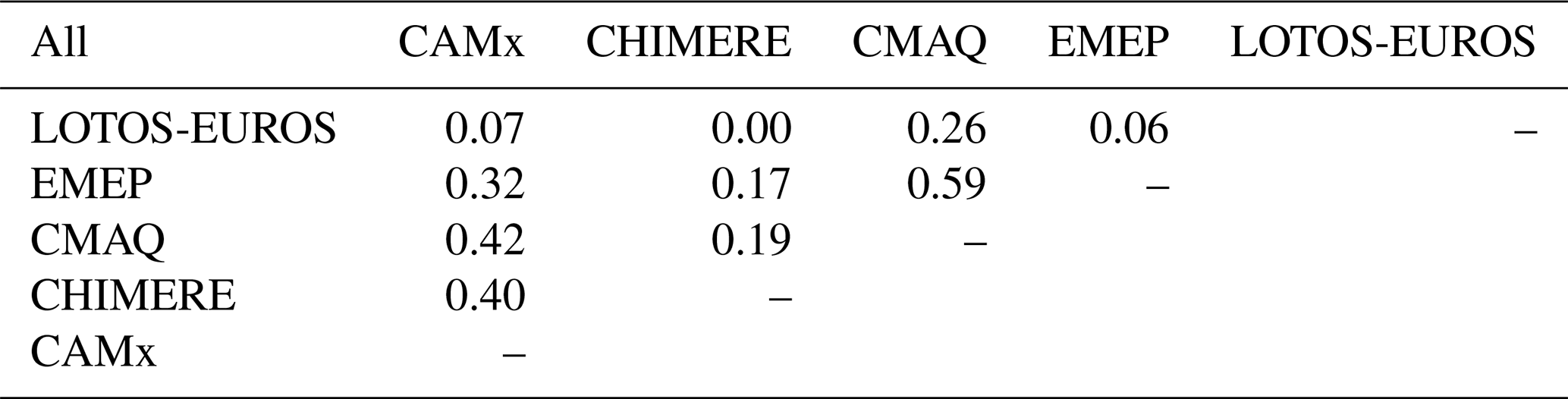
The highest PM2.5 values are simulated by all five models in northern Italy, the Balkan Peninsula, and northern Africa (Fig. 2). The PM2.5 annual mean concentration results show that CHIMERE has the highest annual mean values of 13 to 15 µg m−3 for the eastern part of the domain and over water, whereas LOTOS-EUROS displays the lowest values with 2.0 to 4.0 µg m−3 in most regions (Fig. 2). CMAQ, CAMx, and EMEP show similar model PM2.5 outputs with diverse values distributed between 2.0 and 11 µg m−3 over the domain. The ensemble mean value over the whole domain is 8.6 µg m−3 (Fig. 8a). All five models display high PM2.5 concentrations of > 15 µg m−3 in the Po Valley. In this area, Kiesewetter et al. (2015) and Clappier et al. (2021) also simulated high values between 20 and 45 µg m−3 for 2015. As demonstrated in Table 3, the correlation between the base-run model results with all emissions is the strongest between EMEP and CMAQ (R = 0.59) and CAMx and CMAQ (R= 0.42). In Fink et al. (2023), a high correlation was found between CAMx- and CHIMERE-simulated NO2 and O3 concentrations because both models used the same meteorology. Nevertheless, the present study reveals that particle chemistry causes results that differ more due to a higher complexity in the calculations.
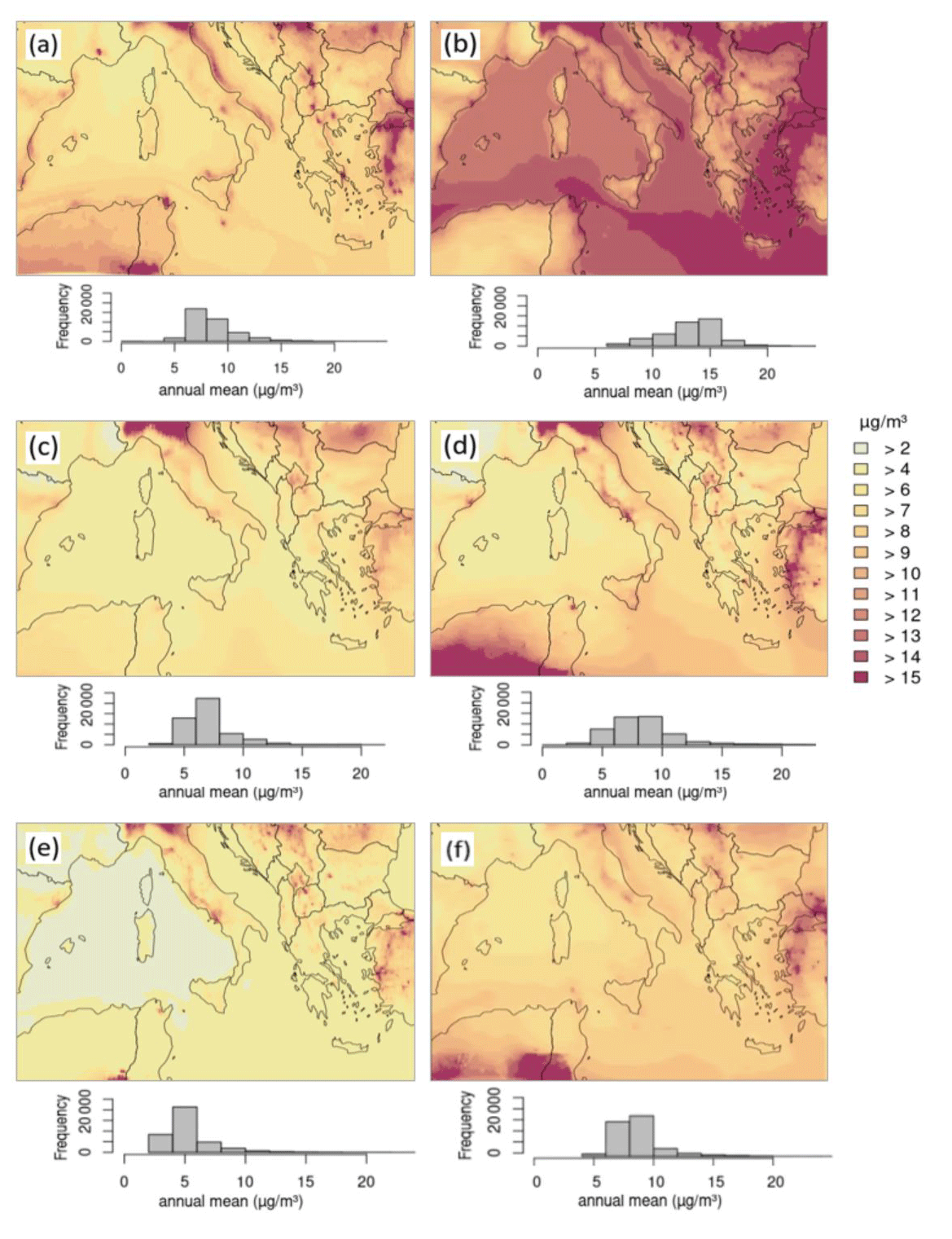
Figure 2Annual mean PM2.5 total concentrations for (a) CAMx, (b) CHIMERE, (c) CMAQ, (d) EMEP, and (e) LOTOS-EUROS, as well as for the (f) ensemble model mean. Below the domain figures are the respective frequency distributions displayed for the annual mean PM2.5 concentrations, referring to the whole model domain.
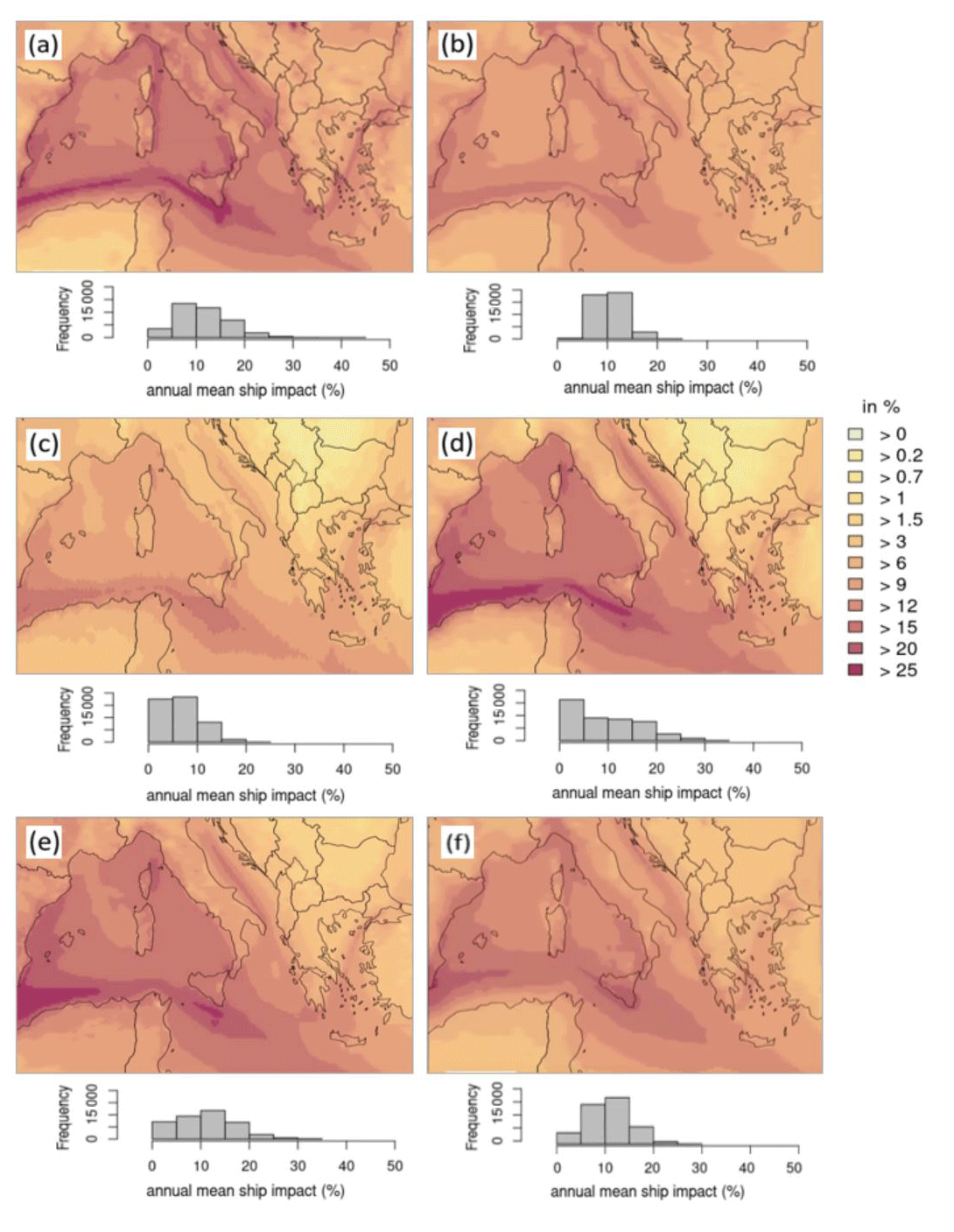
Figure 3Annual mean PM2.5 relative potential ship impacts for (a) CAMx, (b) CHIMERE, (c) CMAQ, (d) EMEP, and (e) LOTOS-EUROS, as well as for the (f) ensemble model mean. Below the domain figures are the respective frequency distributions displayed for the annual mean PM2.5 potential ship impacts, referring to the whole model domain.
The potential impacts of PM2.5 from ships simulated by CAMx, LOTOS-EUROS, and EMEP have the largest areas with values of up to 25 % at the main shipping routes (Fig. 3). CMAQ and CHIMERE have a potential shipping impact of 15 % along the main shipping lines close to the African coast. This impact is lower than that shown in other studies. Aksoyoglu et al. (2016) found the highest impacts of 25 % to 50 % of total PM2.5 concentrations when using CAMx along the main shipping routes. Sotiropoulou and Tagaris (2017) used CMAQ for simulations and stated that emissions from shipping are likely to increase PM2.5 concentrations during winter by up to 40 % over the Mediterranean Sea, while during summer, they simulated an increase of more than 50 %. In both studies, the modeled year is 2006, which might explain the deviation from the present study as using a different year. Regarding coastal areas in the present study, potential shipping impacts reaching 12 % to 15 % are simulated.
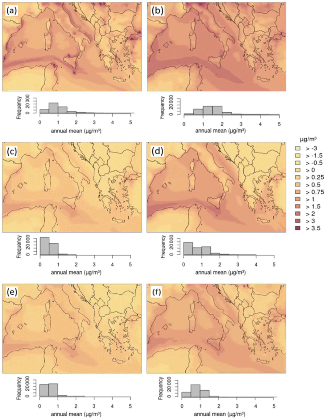
Figure 4Annual mean PM2.5 absolute potential ship impacts for (a) CAMx, (b) CHIMERE, (c) CMAQ, (d) EMEP, and (e) LOTOS-EUROS, as well as for the (f) ensemble model mean. Below the domain figures are the respective frequency distributions displayed for the annual mean PM2.5 potential ship impacts, referring to the whole model domain.
Regarding the absolute potential impacts of ships at the main shipping routes, CAMx, CHIMERE, and EMEP show values of 2.0 µg m−3, and the values simulated by CMAQ and LOTOS-EUROS are between 0.5 and 1.0 µg m−3 (Fig. 4). The median of the ensemble mean is 0.85 µg m−3 (Figs. 4 and 8). Aksoyoglu et al. (2016) simulated similar shipping impacts with CAMx, with values mainly between 0.5 and 1.0 µg m−3.
The sea salt concentrations might partly give an explanation for the differing PM2.5 concentration distribution among the models. The annual mean sea salt (NaCl) concentration in fine and coarse PM showed the highest values for CHIMERE, which might be an explanation for the high PM2.5 absolute concentration (Supplement Fig. S1). The LOTOS-EUROS sea salt displayed the lowest concentrations; the overall PM2.5 concentration is also the lowest compared with the other CTMs. The sea salt concentration was the highest (up to 7.0 µg m−3) over the sea in areas with high surface wind speeds for CHIMERE, CMAQ, EMEP, and LOTOS-EUROS (Fig. S2). This can be confirmed by the correlation between wind speed and sea salt at several points over water for CMAQ, EMEP, and LOTOS-EUROS (Fig. S3; Table S1 in the Supplement). CAMx is excluded from the analysis since sea salt is only present in fine PM.
Solazzo et al. (2012) demonstrated that the chemical components SO, NO, and NH were better reproduced by nine CTMs than the total PM2.5. They concluded from this result that other components (e.g., organic aerosols) could be simulated with less accuracy than inorganic components.
Table 3Correlations between models for the PM2.5 base runs of the whole domain (all grid cells), based on daily PM2.5 total concentration data.
3.3 Precursors
High amounts of NH3, HNO3, SO2, and NO2 are expected to lead to higher values of the aerosol particles composed of NH, NO, and SO. The modeled spatial distributions of these precursors can be found in the Supplement (HNO3: Figs. S4–S6; NH3: Figs. S8–S10; SO2: Figs. S11–S13; and NOx: Figs. S14–S16).
The highest annual mean HNO3 concentration among the base runs is found in the CAMx and CHIMERE simulations over water (2.0 to 5.0 µg m−3); over land, the values are between 0.0 and 1.5 µg m−3, and those in coastal areas reached 2.0 µg m−3 (Fig. S4). The absolute potential ship impact is also the highest in CAMx and CHIMERE at the main shipping routes and over water areas (1.0 to 3.0 µg m−3). The relative potential ship impact on the total HNO3 ranges from 60 % to 85 % along the main shipping routes simulated by CAMx, CMAQ, and EMEP (Fig. S4). These impacts are slightly lower for CHIMERE and LOTOS-EUROS (60 % to 75 %).
The high HNO3 concentrations simulated by CAMx and CHIMERE might be traced back to the NO2 concentrations; these two models also show higher NO2 concentrations than the other CTMs (Fig. S14; Fink et al., 2023). This can be explained by the fact that HNO3 is a major NO2 sink, especially during daytime. NO2 is primarily emitted from anthropogenic fossil fuel burning but also from natural sources (i.e., soil emissions, biomass burning, lightning). During daytime, the main NO2 removal mechanism is oxidation by hydroxyl (OH) radicals to form HNO3 (Seinfeld and Pandis, 1998). It can be concluded that in areas with shipping, more NO2 enters the atmosphere; the total NO2 concentration increases; and as a result of the subsequent reactions, the HNO3 concentration also increases. The HNO3 : NO2 ratio can be used to normalize the data (Fig. S7). The ratio displays low values over land and along the main shipping routes, indicating that in these areas, both the HNO3 and the NO2 concentrations are high. A low HNO3 : NO2 ratio could also mean that only a small amount of OH is present, especially in areas with a low O3 concentration.
After its formation, HNO3 can react with NH3 to be neutralized and to form particles when NH3 is in excess. The annual mean NH3 for the base case shows very similar patterns and values among all models (Fig. S8). The highest concentrations of NH3 with all emission sources are located over land areas with values up to 2.5 µg m−3, which can be traced back to agriculture, the main source of NH3 emissions (Behera et al., 2013). Over water areas, the NH3 concentration is very small, typically between 0.0 and 0.3 µg m−3, except for the slightly higher results modeled by LOTOS-EUROS, with values between 0.2 and 0.8 µg m−3. Negative potential ship impacts (−0.01 to −1.0 µg m−3 and −2.5 % to −150 %; Figs. S9 and S10) are found for the whole domain in all five models. The relative ship impacts are the lowest at the main shipping routes for CAMx and EMEP. The spatial distribution of the NH3 relative ship impact is opposite to the simulated HNO3 values at the main shipping routes, with low NH3 and high HNO3 values. These results indicate that available NH3 reacts directly with HNO3 to form particles (i.e., NH4NO3). Thus, NOx emissions from shipping lead to HNO3 formations and subsequent NH3 consumption; e.g., shipping impacts on NH3 concentrations are usually negative.
The CAMx simulations show the highest SO2 concentrations with more than 10 µg m−3 in some areas in western Turkey, in urban areas, and along major shipping lanes (Fig. S11). The results from the other four CTMs display high values around the Bosporus and in some areas over the Balkan Peninsula with values of 11 µg m−3 and much lower concentrations along the main shipping routes. The potential ship impacts are similarly high in CAMx and CHIMERE (1.0 µg m−3; 85 % of the total concentration; Figs. S12 and S13), with the highest values along the major shipping route north of the African coast. The CMAQ, EMEP, and LOTOS-EUROS results display similarly high values but only in small areas. The modeled year is 2015, so the global 0.5 % sulfur cap of marine fuels was not yet effective. Heavy fuel oils with sulfur contents reaching 3.50 % were used until 2020 to power ships; thus, the SO2 emitted from ships in the present study is still high, and it can be expected that it has a large impact on secondary particle formation.
3.4 Inorganic aerosol species
3.4.1 Concentrations
In the Northern Hemisphere, secondary inorganic ammonium, sulfate, and nitrate aerosols represent a large fraction of the PM2.5 composition (Jimenez et al., 2009). Ammonium preferentially binds to SO in atmospheric aerosols in the form of (NH4)2SO4. NH4NO3, on the other hand, is formed in areas characterized by high-NH3 and high-HNO3 conditions and low-H2SO4 conditions. The results of the CTMs with regard to these three particle species and their potential ship impacts are considered in the following section. The spatial distributions of the total concentrations and absolute potential ship impacts of the individual species can be found in the Supplement (NH: Figs. S17 and S18; SO: Figs. S19 and S20; and NO: Figs. S21 and S22). The spatial distribution of the relative potential ship impact is shown in Figs. 5 to 7.
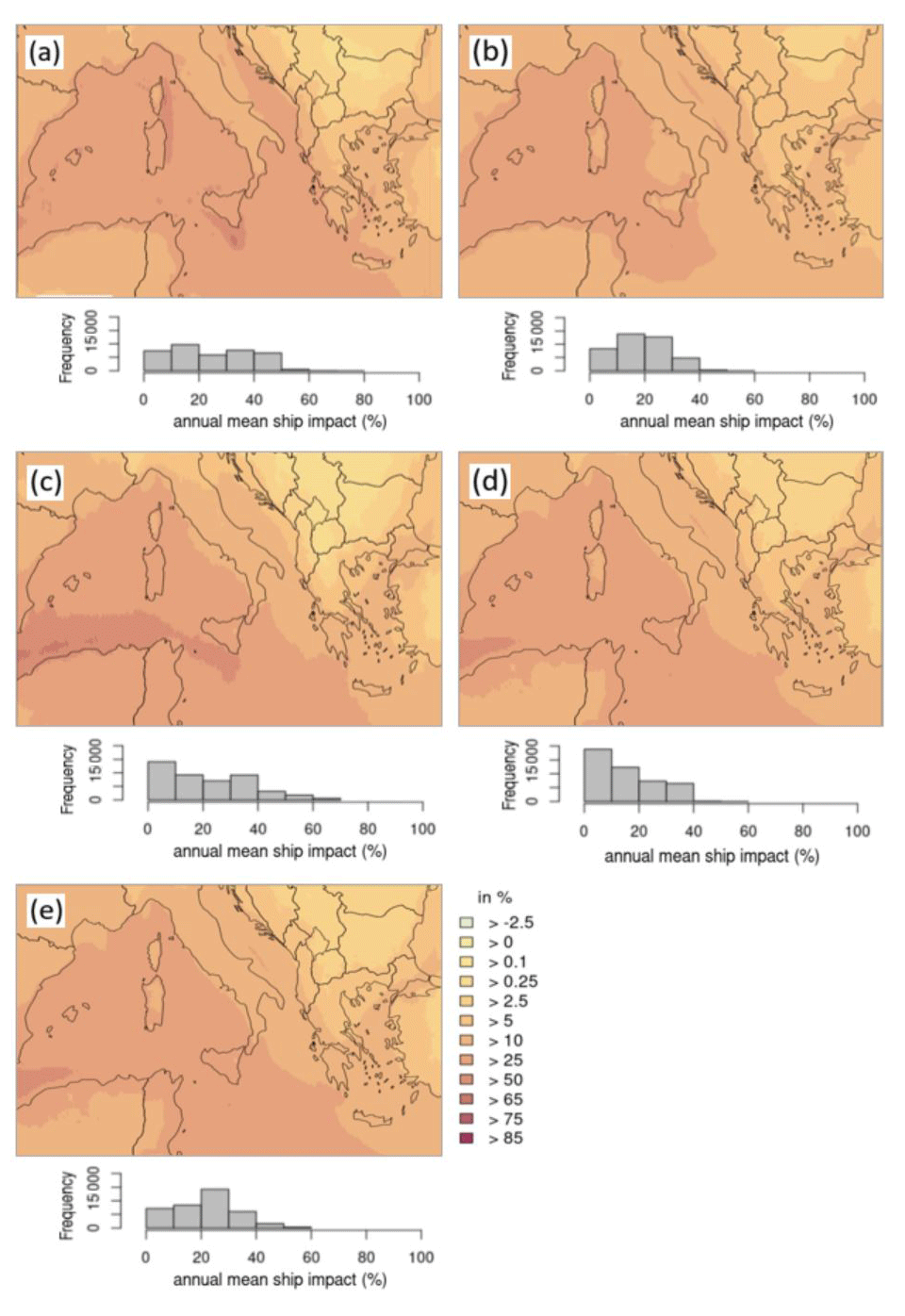
Figure 5Annual mean NH relative potential ship impacts for (a) CAMx, (b) CHIMERE, (c) CMAQ, (d) EMEP, and (e) LOTOS-EUROS. Below the domain figures are the respective frequency distributions displayed for the annual mean NH potential ship impacts, referring to the whole model domain.
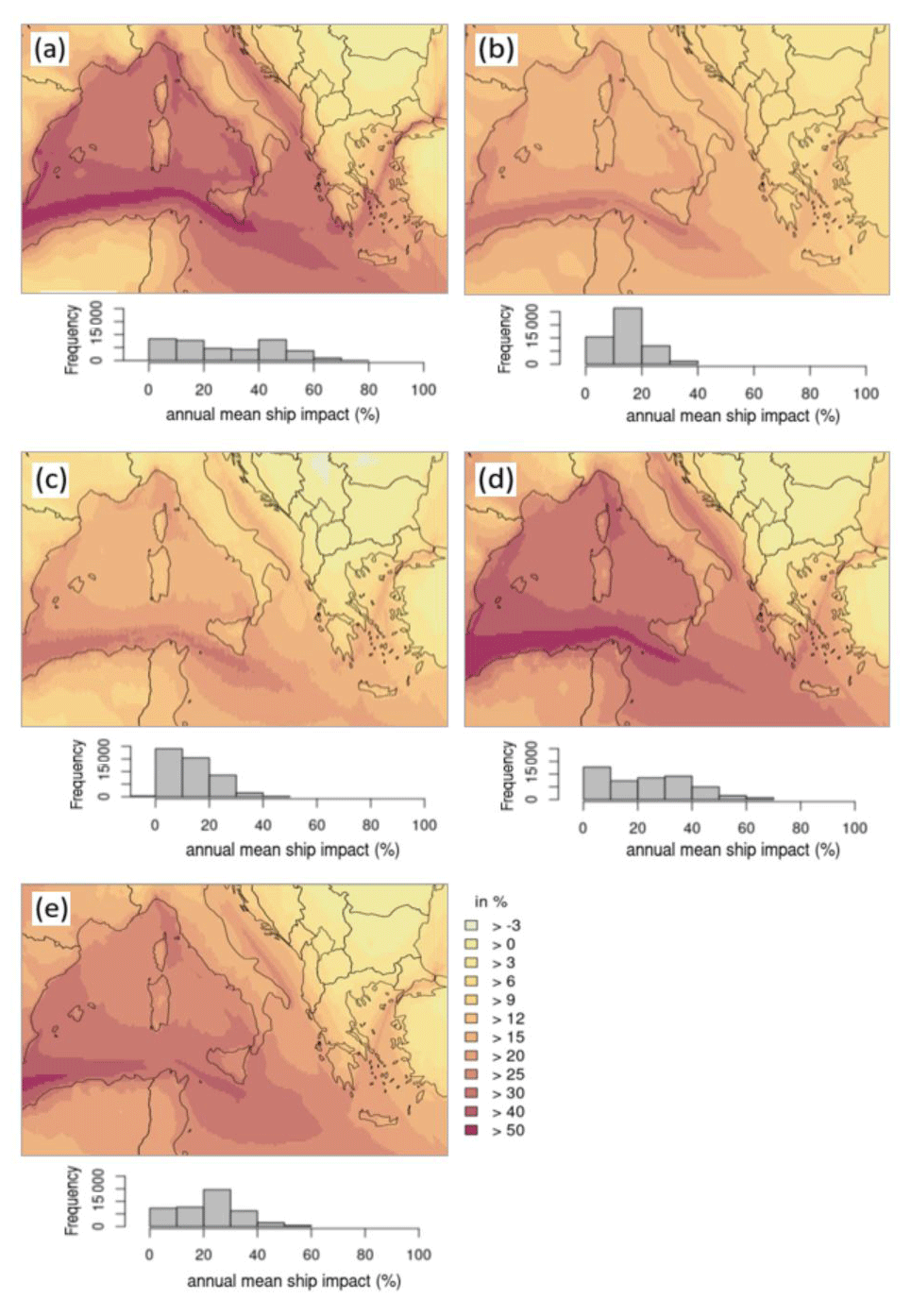
Figure 6Annual mean SO relative potential ship impacts for (a) CAMx, (b) CHIMERE, (c) CMAQ, (d) EMEP, and (e) LOTOS-EUROS. Below the domain figures are the respective frequency distributions displayed for the annual mean SO potential ship impacts, referring to the whole model domain.
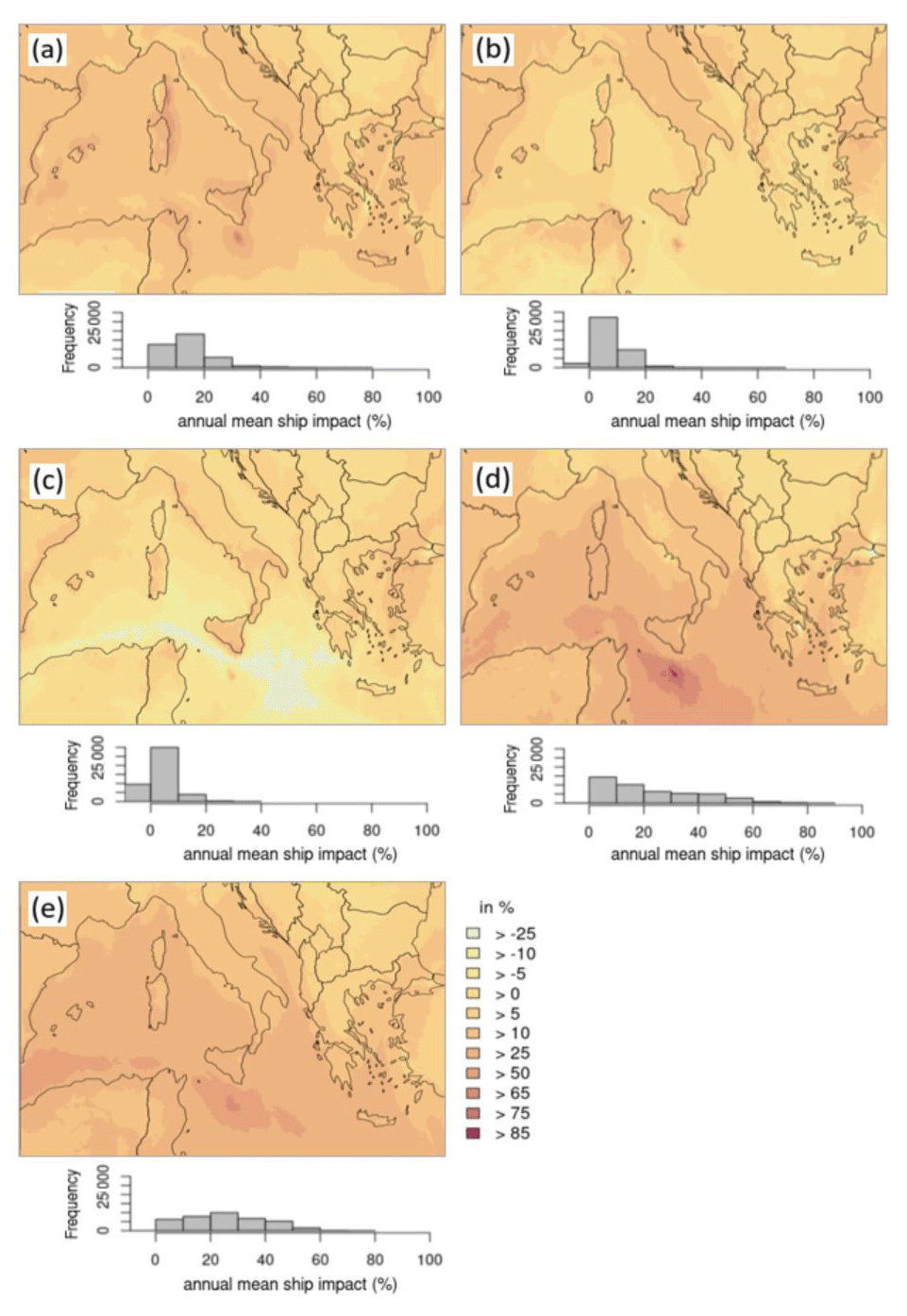
Figure 7Annual mean NO3 relative potential ship impacts for (a) CAMx, (b) CHIMERE, (c) CMAQ, (d) EMEP, and (e) LOTOS-EUROS. Below the domain figures are the respective frequency distributions displayed for the annual mean NO3 potential ship impacts, referring to the whole model domain.
The spatial distribution of NH shows that the lowest total annual mean can be found mainly in the southwestern part of the domain (approximately 0.0 µg m−3) and the highest in the Po Valley and Bosporus (1.5 µg m−3, Fig. S17). The relative ship impacts are very similar for all models (0.25 % to 5.0 % over land, 10 % to 25 % over water; Fig. 5) as well as for the absolute ship impact (Fig. S15). Aksoyoglu et al. (2016) simulated NH values between 0.0 and 0.2 µg m−3 in the Mediterranean region, with higher concentrations (0.4 µg m−3) in the Po Valley. This is within the same range of concentrations in the present study. Ge et al. (2021) used the EMEP model to simulate global particle species concentrations and compared them with measured concentrations. They showed in their study that the NH concentrations simulated in Europe in 2015 were overestimated by a factor of 2 compared with the actual measured NH concentrations. The measurements displayed a mean of 0.45 µg m−3. The ensemble mean for NH in the present study (0.6 µg m−3, Fig. 8a) is in good agreement with these measurements. However, a previous study on measured compared with simulated aerosol distribution with the CMAQ model displayed a slight underestimation of NH (Matthias, 2008).
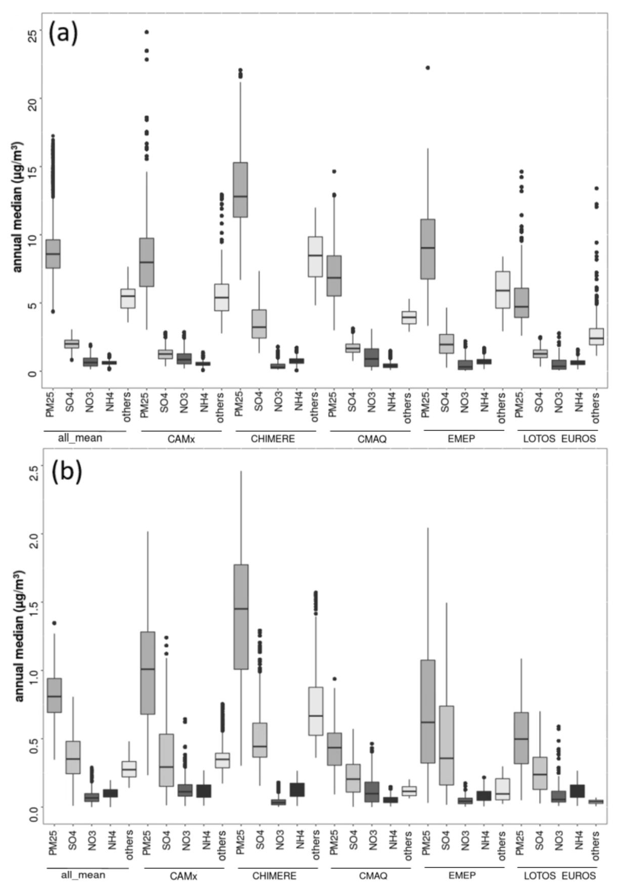
Figure 8(a) Boxplots for concentrations of PM2.5 and the PM2.5 components SO, NO3, NH, and “others” as simulated by the five CTMs. The ensemble mean is “all_mean”. Others are calculated as PM2.5 minus the sum of SO, NO3, and NH. Data are based on the whole domain (all grid cells) and hourly data for all emission sources (“emisbase”). (b) The same as (a) but for ships only.
The NH proportion to the total PM2.5 is similar among all models (5.6 % to 7.8 %; Fig. 8a, Table 4), and only LOTOS-EUROS displayed a relatively high share (12.2 %). This pattern is similar for the ship impacts, where all models show proportions between 9.1 % and 12.6 %, but higher values are simulated by LOTOS-EUROS (23.5 %; Fig. 8b, Table 5).
SO is the oxidation product of SO2, which is primarily emitted by anthropogenic processes such as fossil fuel combustion, petroleum refining, and metal smelting (Zhong et al., 2020). In the present study, SO is the main contributor to the total PM2.5 mass (Fig. 8, Table 4). Especially in the model ensemble mean for the absolute ship-related concentrations, SO makes up 44.6 % of PM2.5 (Fig. 8b, Table 5). The annual mean SO total concentration is the highest for CHIMERE in the eastern part of the domain, reaching 6.0 µg m−2. EMEP displays a SO concentration within the ranges of the other models, CAMx, CMAQ, and LOTOS-EUROS, in the western part of the domain. These models show very similar spatial distributions with concentrations of up to 2.0 µg m−3. The median ensemble mean for the run with all emission sources is 2.0 µg m−3. This ensemble mean is low in comparison with the results of Solazzo et al. (2012); they found a mean value of 6.0 µg m−3 but considered a larger European area that included the areas with the highest SO concentrations in Europe. For this larger area, Solazzo et al. (2012) found that the models used underestimated SO by 7 % to 17 %.
In the present study, the relative potential ship impact on the total SO is the lowest over land, with 0 % to 3.0 %, and higher in coastal areas, with values from 6 % to 20 % (Fig. 6). Along the main shipping routes it is the highest, reaching 50 % for CAMx, EMEP, and LOTOS; for CHIMERE and CMAQ, it is lower, with values reaching 30 %. Aksoyoglu et al. (2016) showed similar relative potential ship impacts of 50 % to 60 % in the western Mediterranean. In their study, values were between 0.0 to 1.0 µg m−3 over land areas, but over water along the main shipping routes they were the highest at 2.2 µg m−3.
Mallet et al. (2019) traced back higher SO in the eastern part of the domain due to westerly winds. In the present study, we found this higher concentration for SO in the eastern part of the Mediterranean as well. In Lampedusa, they found ammonium sulfate contributed 63 % to PM1 mass, followed by organics (Mallet et al., 2019). In our study, the organics/others had the highest share of total PM2.5 when considering all emission sources, followed by sulfate and ammonium. In the present study, CTM systems simulated lower values for ship impacts; over land, they are 0.0 to 0.03 µg m−3, and along the main shipping routes, they reached 0.9 µg m−3. Regarding the absolute ship impacts on SO, the model simulations display similar concentrations and are slightly lower for CMAQ and LOTOS-EUROS (Fig. S20) compared with the other models. Especially over water areas, large areas with considerable SO2 and SO concentrations can be seen. Because NH is preferentially bound to SO in atmospheric aerosols to form (NH4)2SO4, in areas over water, less NH4NO3 forms.
Im et al. (2014) suggested in their intercomparison study that over Europe, SO levels were underestimated by most models; only a few models overestimated SO concentrations in Europe. The underestimating models were WRF-Chem models, and the SO underestimations were attributed to the absence of SO2 oxidation in cloud water in the heterogeneous phase.
The highest annual mean NO total concentrations are simulated over land areas, especially over Italy and in the Balkan states (> 2 µg m−3; Fig. S18), and the lowest concentrations are over the sea. CAMx, CMAQ, and LOTOS-EUROS show higher concentrations compared with results derived from CHIMERE. The concentrations over water are lower than those over land. The ensemble median of all CTMs over the whole domain is 0.63 µg m−3 (median value; Fig. 8a). The absolute potential impacts of ships on the total NO concentrations are similar among all models, displaying values mainly between −0.005 and 0.15 µg m−3; only CMAQ demonstrates relatively low values along the main shipping routes (−0.5 µg m−3), and CAMx has higher values (1.0 µg m−3) in some coastal areas (Fig. S19). This can be explained by higher SO concentrations derived from SO2 emissions. Sulfate replaces nitrate as long as the ammonia concentration is low. In model simulations with ships, NO can decrease because ammonia is already taken from sulfur emissions from ships. Aksoyoglu et al. (2016) found similar results for the Mediterranean Sea considering the NO concentrations, with values between 0.0 µg m−3 and 0.2 µg m−3. Im et al. (2014) showed that simulated NO levels were overestimated by most of the CTMs by more than 75 %. Higher concentrations over water than over land due to NH4NO3 formation are found in areas characterized by high-NH3 and high-HNO3 conditions and low-H2SO4 conditions. In the present study, the relative potential ship impacts on NO display contradicting tendencies among the models (Fig. 7). The CAMx, EMEP, and LOTOS model results are similar, with relative potential ship impacts over land from 0.0 % to 5.0 % (in the Balkan states), those in coastal areas and Italy from 10 % to 25 %, and those along main shipping routes from 50 % to 65 % or even up to 85 %. CHIMERE and CMAQ display lower relative potential ship impacts. For CMAQ, the impact is negative along the main shipping routes, at −25 %. Sulfur dioxide or ammonia might lead to a negative NO impact because the NO2 emissions from ships would make a positive contribution to nitrate formation. Therefore, without ships, an (NH4)2SO4 should be formed, which is more stable than NH4NO3. These low values in the aerosol species for CMAQ but higher values for EMEP, CAMx, and LOTOS represented the PM2.5 ship impacts and might partly explain the deviations in PM2.5. Furthermore, in CMAQ the coarse mode in nitrate and ammonium has a larger share compared with the other CTMs. A more detailed discussion is given in Sect. 4.
Regarding the PM2.5 composition, the share of other particles, which contain mainly organics but also, e.g., sea salt, is the highest compared with the inorganic species (Fig. 8). Nevertheless, the particle composition revealed varying distributions in the ship-related PM2.5 concentration. Here, inorganic particle species have relatively high percentages compared with organic aerosols. In some cases, sulfate has an even higher share of the total PM2.5 than other particles.
The seasonal variability in particle species shows that NO is more temperature dependent than SO and NH. NO is higher in winter and spring but lower in summer and autumn. This pattern can be found in all CTM simulations. For PM2.5, on the other hand, no discernible pattern is found regarding seasonal variability. In particular, the ensemble mean PM2.5 concentration remained within the same range in all seasons.
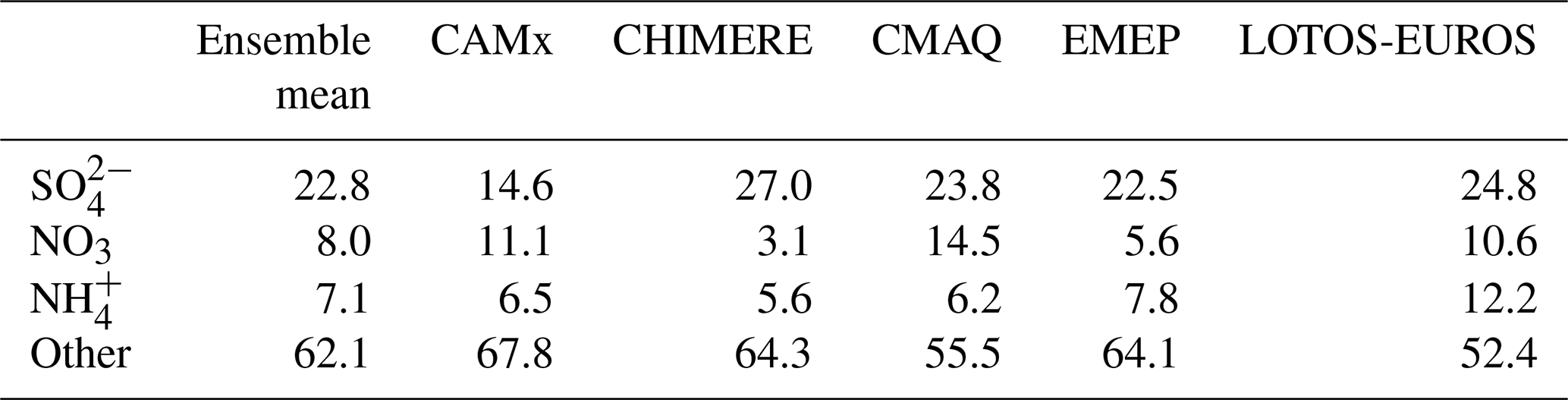
Table 5Relative particle species of total shipping-related PM2.5.
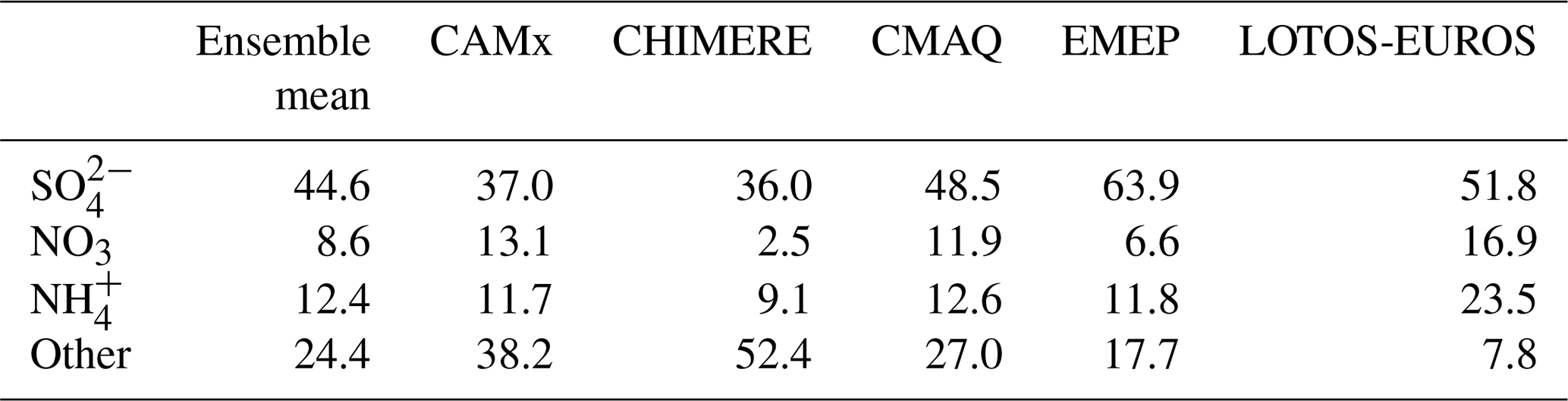
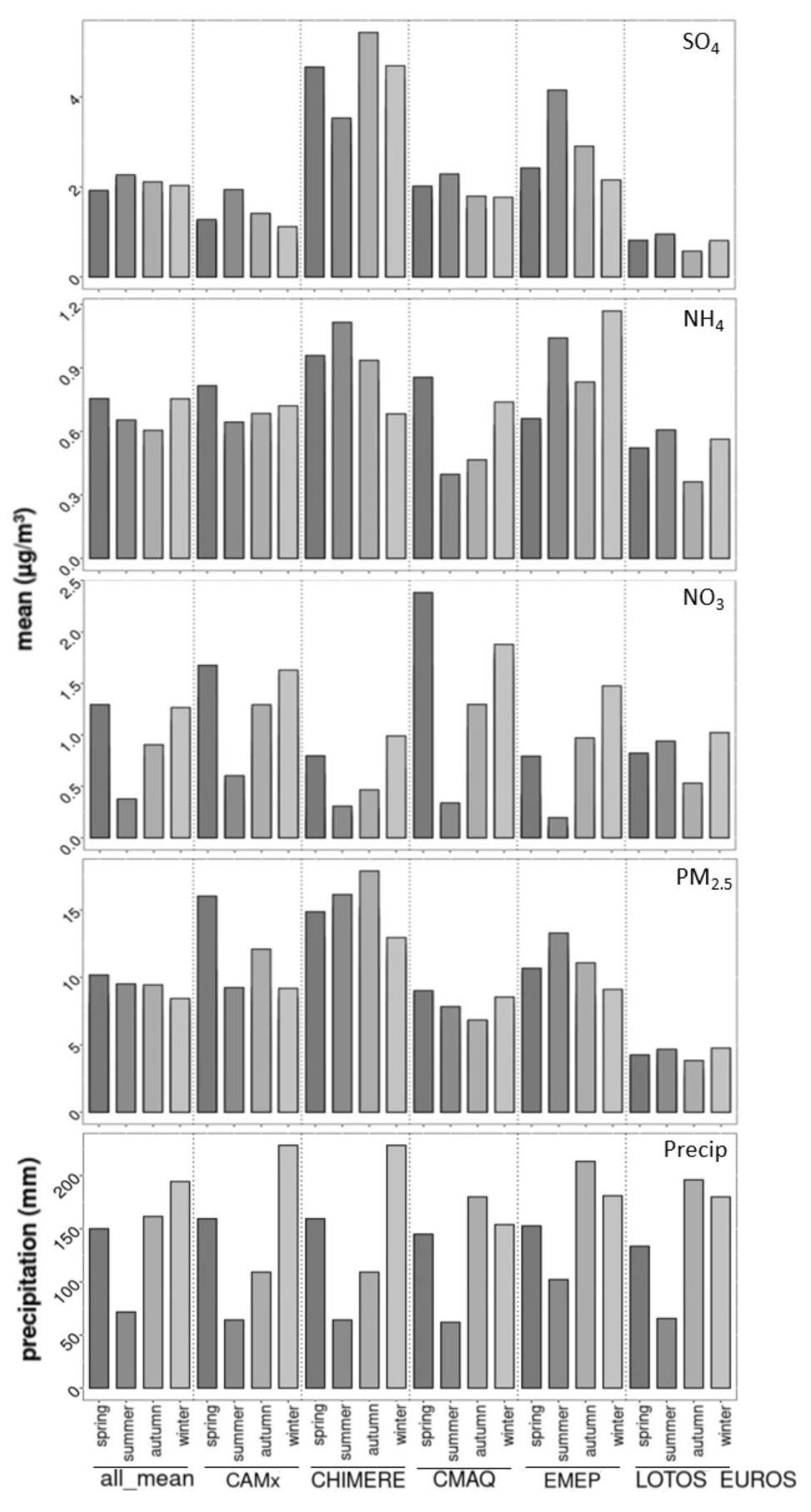
Figure 9Concentration of particle species and precipitation divided by seasons and CTMs. “all_mean” displays the model ensemble. Spring: March, April, May; summer: June, July, August; autumn: September, October, November; winter: December, January, February. Concentration is based on the annual median over the whole domain. Precipitation displays the seasonal sum (in mm).
3.4.2 Wet deposition
Wet deposition can provide indications of the fate of particles. EMEP does not deliver separate deposition files for individual particle species but for reduced and oxidized nitrogen. Thus, EMEP is not considered when analyzing wet deposition in this study.
Regarding the spatial distribution of NH wet deposition, the highest annual sums are displayed by CMAQ and LOTOS-EUROS (up to 250 mg m−2 yr−1 over land; up to 50 mg m−2 yr−1 over water; Fig. S23). CAMx and CHIMERE show a similar spatial distribution with values mainly between 10 and 25 mg m−2 yr−1. CAMx and CHIMERE used the same meteorology data, but despite this the seasonal distribution of wet deposition differs (Fig. 10). An explanation for this differing behavior might be provided by the scavenging mechanisms. In CHIMERE the in-cloud mechanism for deposition of particles is assumed to be proportional to the amount of water lost by precipitation. In CAMx, the in-cloud scavenging coefficient for aqueous aerosols is the same as for the scavenging of cloud droplets. Below the cloud, CHIMERE uses a polydisperse distribution following Henzig et al. (2006), whereas in CAMx for rain or graupel the collection efficiency is calculated as in Seinfeld and Pandis (1998). The other possible explanation is that all the emissions in CAMx are emitted in the first layer and in CHIMERE it depends on the emissions distribution.
Regarding the wet deposition of sulfate, the annual totals for all emission sources are the highest over the Balkan Peninsula in the CMAQ and LOTOS-EUROS model outputs (300 to 800 mg m−2 yr−1; Fig. S24). For CAMx over land areas, the values reach 300 mg m−2 yr−1, and the lowest totals over land can be seen in the CHIMERE results (0.0 to 50 mg m−2 yr−1). Over water, these values are low in all model outputs (50 to 150 mg m−2 yr−1), except in CHIMERE, where, in contrast to the other models, the highest wet deposition was found over water.
The wet deposition of NO is the highest for CMAQ (> 400 mg m−2 yr−1) over the whole domain (Fig. S25). For CAMx and LOTOS-EUROS, it is generally lower, with most areas displaying 25 to 50 mg m−2 yr−1. The lowest wet deposition of nitrate is shown in CHIMERE outputs with values not exceeding 50 mg m−2. Regarding the sum for the whole year, the highest values are found for CMAQ (northern Italy and the Balkan Peninsula, where the urban-area values reached 400 mg m−2 yr−1). Over water, deposition is lower than over land in the results of all CTMs. Lower wintertime precipitation in CMAQ compared with the other models might lead to high particle concentrations as well as high deposition due to low dilution (Fig. 10).
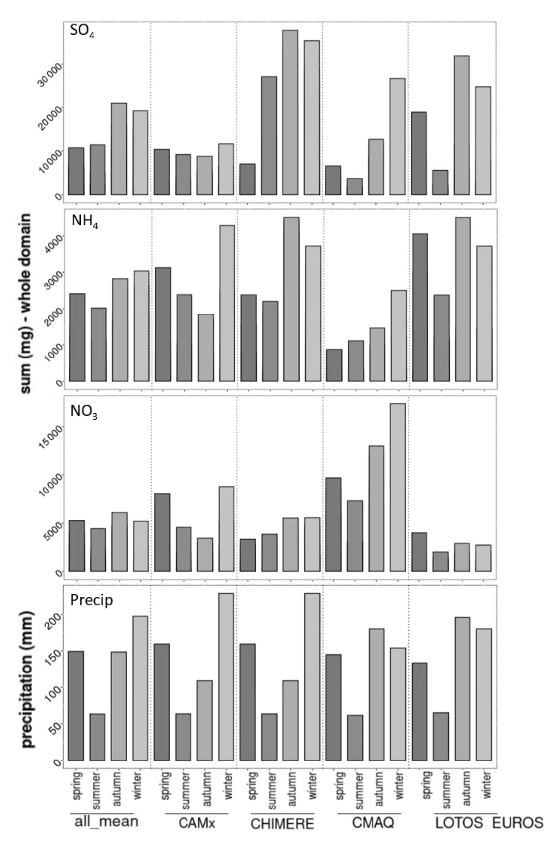
Figure 10Wet-deposition sum (mg per season) of particle species and precipitation divided by seasons and CTMs. “all_mean” displays the model ensemble. Spring: March, April, May; summer: June, July, August; autumn: September, October, November; winter: December, January, February. Wet deposition is based on the annual sum over the whole domain. Precipitation displays the seasonal sum (in mm).
Wet deposition depends mainly on the ability of the models to predict the amount, duration, and type of precipitation. The precipitation data show that the lowest values are found for CMAQ input data. CAMx and CHIMERE use the same meteorological input data and thus display the same precipitation results, with the highest values in winter. CMAQ and LOTOS-EUROS have precipitation values within a similar range, with the highest values occurring in autumn and winter.
Although the precipitation results in CAMx and CHIMERE are the same, wet deposition differed between these two models, indicating that the concentration as well as model internal mechanisms caused differences rather than the input data. Additionally, in CMAQ, a lower wet-deposition rate is expected for nitrate. There are usually two mechanisms that are important for scavenging in CMAQ: in-cloud and below-cloud scavenging. High wet deposition for nitrate in CMAQ outputs might be traced back to efficient below-cloud scavenging of coarse-mode particles containing nitrate, through which the wet deposition can be high despite precipitation in similar ranges to other models. Furthermore, the deposition of particulate nitrate crucially depends on the reactive uptake of HNO3 to larger particles (Karl et al., 2019) because coarse-mode particles are removed much faster than fine-mode particles.
Various reasons for deviations in PM2.5 concentrations among regional CTM systems might be traced back to model-specific calculations.
Regarding PM (coarse and fine for sea salt), an uncertainty among models might be caused by the differences in the calculation of sea salt and dust emissions. Here, both are considered in all CTMs, except for dust in CMAQ. If sodium chloride and dust components are not considered, underestimations of PM and uncertainties in areas near coasts (sea salt) or where dust is important, e.g., Saharan dust in the Mediterranean region, occur, as described in Sect. 3.1. Furthermore, if sea salt and dust are omitted from the pH calculations, it might also cause deviations in sulfur chemistry, as this factor is very sensitive to pH.
In the CMAQ runs dust was considered at the model boundaries but dust emissions were not included. The Mediterranean region is frequently affected by Saharan desert dust (Palacios-Peña et al., 2019), but the main source region for this dust emission is not included in the model domain; thus the dust coming from the boundary can be seen as sufficient for the CMAQ model run. Generally, the boundary conditions for dust and sea salt in CAMx and CHIMERE were produced by offline models that run on meteorological fields from GEOS-5, GEOS DAS, and MERRA. For CMAQ and LOTOS-EUROS these boundary conditions were produced within the boundary condition calculations. Boundary conditions of EMEP are developed from climatological ozone-sonde datasets.
All models used offline meteorology in which the ABL heights were calculated. Annual medians of the atmospheric boundary layer heights at 16:00 and 04:00 UTC were compared among the models. The comparison of spatial distribution of ABL heights at 16:00 and 04:00 shows that over water, the ABL heights do not have much variability in all models (Figs. S26 and S27). The lowest ABL height over water was used for CHIMERE. This corresponds to the high PM2.5 concentrations simulated by this model over water. Over land, the comparison of spatial distribution from 16:00 to 04:00 displays more variable ABL heights: during nighttime the ABL heights are up to 200 m, whereas during daytime the heights increase to 1000 m or higher (Figs. S26 and S27). Over land the input in CAMx, CHIMERE, CMAQ, and LOTOS-EUROS has a higher median ABL at 16:00, whereas in EMEP it is the opposite, with the highest median at 16:00 mainly being over water areas. However, there was not a large deviation in the PM2.5 concentration simulated by EMEP from concentrations received from other models. Generally, due to ABL dynamics, deviations between measured and simulated data can be expected because measurement stations were chosen close to the coast, which leads to uncertainties. In these areas, the measurements are influenced by air masses either coming from water or coming from land. In addition, measured data were received from one measurement point, which is hardly representative of a whole grid cell of 12×12 km2.
The treatment of dust and sea salt, as well as the boundary conditions used, has an effect on the analysis and comparison of PM results because these parameters are part of the PM2.5 formation but differ among the models. Regarding the CTM performances, reasons for underestimations of PM2.5 have already been discussed in previous studies: for CAMx, Pepe et al. (2019) linked these underestimations to meteorological parameters and to the overestimation of the vertical mixing in the lower atmosphere. Tuccella et al. (2019) found underestimations of PM2.5 in the CHIMERE model and explained these by an excess of wet scavenging in the model. An excess of wet scavenging in CHIMERE compared with the other CTM systems is not found in the present study; thus it cannot be used as an explanation for deviations here. In EMEP, which differs from the other CTM systems, the MARS module was used to calculate the equilibrium between the gas and aerosol phases; this model does not treat sea salt or dust, leading to underestimations of PM2.5. Kranenburg et al. (2013) linked the underestimation of particulate matter in LOTOS-EUROS to the missing descriptions of SOA processes in the model. Thus, various reasons and combinations of reasons can lead to underestimations of PM2.5 in the CTM systems used herein. For a better understanding, the inorganic particle species are considered in the present study. Consideration of inorganic and organic particles could lead to more uncertainties. Moreover, in shipping emissions the inorganic aerosols display a higher share.
A large part of PM2.5 is secondary; therefore underestimations can be linked to underestimations of precursors, e.g., NO2. This has already been shown in the first part of this intercomparison study, where all five CTM systems underestimated measured NO2 (Fink et al., 2023). But SO2 is also usually underestimated by CTMs, as shown in previous studies (e.g., Eyring et al., 2007). Four out of five CTM systems underestimate the actual measured PM2.5 concentration in the present study. Gaseous precursors like SO2 and NO2 need to be oxidized before they can form particles in reactions with ammonia. The hydroxyl radical (OH) is the main oxidant. The amount of available OH can be analyzed when the NO2 concentration is set in relation to HNO3 and NO (Fig. S28). This gives an indication of the OH availability. In ship plumes OH is consumed fast; therefore values are low along the shipping lanes. In regions with lower NO2 concentrations, more OH is available, and HNO3 is efficiently formed. In the present study, the HNO3 was similar within all five CTM systems (Fig. S5).
One reason for the differences in HNO3 might be traced back to the amount of cloud droplets, since HNO3 is resolved in them. The dissolution of gases in droplets is usually assumed to be irreversible for HNO3 and NH3 in CTMs; thus, the amount of formed ammonium nitrate mass depends on the amount of HNO3 or the cloud droplets. This could in the end lead to the deviation among the CTM-simulated HNO3.
The preference of NH to bind to SO in atmospheric aerosols to form (NH4)2SO4 explains why in some models NO displays relatively low values when the SO concentration is high. CHIMERE, for instance, has an NO share of 3.1 % to the total PM2.5 and an SO share of 27.0 %, whereas in the CAMx results, NO has a share of 11.1 % to the total PM2.5 and an SO share of 14.6 %. This is confirmed by the low SO2 concentration and high SO concentration in CHIMERE (Figs. S11 and S19), indicating that sulfate is formed more efficiently compared with CAMx. Furthermore, this leads to lower NO concentrations in the CHIMERE output (Fig. S21). For SO2 and SO the concentration of cloud water and the amount of cloud droplets also play an important role.
Regarding the thermodynamic equilibrium within the models, ISORROPIA and ISORROPIA II mechanisms are used in all CTM systems except EMEP, meaning similar results can be assumed to be obtained from this mechanism. Despite this similarity, differences in concentrations may be a result of differences in available cloud water, vertical mixing, the spatiotemporal distribution of emissions, or aerosol size distributions. EMEP uses the MARS module to calculate the equilibrium between the gas and aerosol phases. Although four of the five models use the ISORROPIA or ISORROPIA II mechanisms for inorganic secondary aerosol formation, many factors within these models still cause significant differences among the model outputs.
The aerosol size distribution also has an impact on the particle species distribution. As displayed in Table 1 (Sect. 2.1), there are two concepts for how the aerosol size distribution is represented within the models: the distribution is either in bins or in log-normal modes. As already discussed in Solazzo et al. (2012), the PM chemical composition differs greatly with the particle size. Consequently, differences in modeling the aerosol size distribution also affect the chemical composition. In CMAQ, for example, large fractions of nitrate and ammonium can be found in the coarse mode where they undergo different removal processes than in the fine mode.
Although there is harmonization in terms of the input emission data in the present study, the internal model mechanisms used to calculate particulate matter lead to differences in the particle species distribution, as discussed in Sect. 3.1. In addition, the calculations of how to determine PM2.5 vary among CTM systems or even within one CTM. As an example, there are two possibilities for calculating PM2.5 within CMAQ: either online during the model run with the PM2.5 module or subsequently by calculating the value as the sum of two modes. These different options lead to different results (as shown by Jiang et al., 2006) and will also affect the particle composition. In the present study, the sum of two modes is used in CMAQ.
Model simulations with relatively high PM2.5 concentrations display higher absolute shipping impacts on PM2.5, as presented in Sect. 3.2. Consequently, relatively low variability in the relative potential ship impacts among the models compared with that of the absolute values could be expected. For a more quantitative evaluation, the relative potential ship impact is plotted against the absolute potential impact. A larger incline of the regression line can be explained by a higher background PM2.5 concentration; thus the relative ship impact is lower for the same concentration increase (e.g., EMEP and CHIMERE) (Fig. S29).
From the ISORROPIA and ISORROPIA II mechanisms, it can be expected that the molar ratios between the acids on the one side (NO and SO) and the base on the other side (NH) are in balance. However, the ratio between SO, NH, and NO shows that the balance in all models except in LOTOS-EUROS is not given for PM2.5; sulfate plus nitrate is much higher compared with ammonium (Fig. S30). This balance is almost perfectly given in LOTOS-EUROS, although both CMAQ and LOTOS-EUROS used the ISORROPIA II mechanism. An imbalance among the inorganic particle species is present, especially at the shipping lanes. Differences in the particle species ratio among the models can be traced back to the differences in the particle size distribution. In contrast to the other models, CAMx only has three species in the coarse mode: coarse others primary, coarse crustal, and reactive gaseous mercury. For NO and SO, the ratio between the fine and coarse mode is calculated for the CTMs (Figs. S31 and S32). NH was not considered here, since it is only in present in the coarse mode in CMAQ. These ratios show that CHIMERE and LOTOS-EUROS only have a small proportion of particles in the coarse mode. For SO in LOTOS-EUROS the coarse particle concentration is zero and for EMEP no SO is present in the coarse mode. In CMAQ a higher concentration of particles is assigned to the coarse mode and also for NH.
The present study has shown that different reasons can cause deviations among the simulated PM2.5 CTM outputs. The major reasons are the differences in the size distribution and how models distribute chemical species between the coarse and fine modes (PM2.5 and PM10). Differences among the modeled PM2.5 concentrations can also be a result of the differences in the height of the lowest model layer and the way in which ship emissions are distributed among the layers. As shown in Fink et al. (2023), the vertical distribution of PM2.5 precursor emissions varies among the models; e.g., in CAMx all shipping emissions are assigned to the lowest layer. This leads to differences in chemical transformations because of different concentration levels close to the source and consequently to deviations among the particle distributions. Furthermore, precipitation differences lead to variations among the model outputs for wet deposition.
The limitations of the present study are that only the chemistry of the lowest layer is evaluated. The model input was standardized as far as possible, but meteorological input data varied and are not compared in detail here. Interactions between fine and coarse particles are only studied to a limited extent, and the same holds for aqueous chemistry, which has an impact on the oxidation mechanisms of sulfur species.
The current work investigates and analyzes the predictions of five different CTM systems for PM2.5 and inorganic particle species (NH, SO, NO) dispersion and transformation in the Mediterranean region. Additionally, the total concentration focus is on the potential ship impact. The results show that four of the five models underestimated the actual measured PM2.5 concentrations at stations close to the European coastline. The relative ship impacts on PM2.5 simulated by the CTMs at the measurement stations are between 5.7 % (CMAQ) and 13.8 % (CAMx). The potential impacts of PM2.5 from ships simulated by CAMx, LOTOS-EUROS, and EMEP have the largest areas with values of up to 25 % along the main shipping routes in the Mediterranean Sea. CMAQ and CHIMERE simulated potential ship impacts of 15 % along the main shipping lines close to the African coast. These impacts are within the range of the ship impacts obtained in other studies.
The spatial distribution of ammonium displays a low total annual mean mainly in the southwestern part of the domain (approximately 0.0 µg m−3) and is the highest in the Po Valley and Bosporus (1.5 µg m−3 ). The ensemble mean of NH (0.6 µg m−3 ) is in good agreement with the measurements provided in previous studies. The relative and absolute ship impacts are very similar for all models (0.0 to 0.06 µg m−3 over land, up to 0.15 µg m−3 over water; 0.25 % to 5.0 % over land, and 10 % to 25 % over water). This indicates that differences among the simulated PM2.5 from ships result from differences in sulfate and nitrate.
The NH proportion to total PM2.5 is similar in all models (5.6 % to 7.8 %), and only LOTOS-EUROS shows a relatively high share (12.2 %). The ship impact pattern is similar; all models display proportions between 9.1 % and 12.6 %, but higher values are simulated by LOTOS-EUROS (23.5 %).
SO is the main contributor to the total PM2.5 concentration regarding shipping emissions only. In the model ensemble mean for the absolute ship concentration, SO accounts for 44.6 % of PM2.5. The annual mean sulfate total concentration is the highest for CHIMERE in the eastern part of the domain, reaching 6.0 µg m−3. CAMx, CMAQ, EMEP, and LOTOS-EUROS simulate a total SO concentration within one range between 0.4 µg m−3 and 2.0 µg m−3 in the western part of the domain. The relative potential ship impacts on the total SO are the lowest over land, with values of up to 3.0 %, and are higher in coastal areas, with values ranging from 6 % to 20 %. Along the main shipping routes, the impacts are the highest, reaching 50 % for CAMx, EMEP, and LOTOS-EUROS; for CHIMERE and CMAQ, they are lower, with values reaching 30 %. Regarding the absolute ship impacts on SO,, the model simulations display similar concentrations and are slightly lower for CMAQ and LOTOS-EUROS. Concentrations are in particular identified over water areas with relatively high SO2 and SO. Because NH preferentially binds to SO in atmospheric aerosols to form (NH4)2SO4, in areas over water less NH4NO3 forms.
The highest annual mean NO total concentrations appear over land areas in the simulations by CAMx, CMAQ, and LOTOS-EUROS, especially over Italy and in the Balkan states (> 2 µg m−3). The lowest concentrations are simulated by CHIMERE. The concentrations over water are lower than those over land areas. The ensemble mean of all CTMs over the whole domain shows a median value of 0.63 µg m−3. Higher concentrations over land than over water are expected due to NH4NO3 formation in areas characterized by high-NH3 and high-HNO3 conditions and low-SO conditions.
The relative potential ship impact on NO differs among the models. The CAMx, EMEP, and LOTOS-EUROS results are similar; the relative potential ship impacts over land range from 0.0 % to 5.0 % (in the Balkan states), those in coastal areas and Italy range from 10 % to 25 %, and those along main shipping routes range from 50 % to 65 % or even reach 85 %. CHIMERE and CMAQ show lower relative potential ship impacts for NO. For CMAQ, the impacts are the lowest along the main shipping routes; nitrate is even reduced by 25 %. Low values in nitrate can be explained by the preference to form (NH4)2SO4; thus nitrate stays in the gas phase or is transferred to the coarse mode. These low values for SO and NO in CMAQ but relatively high values for EMEP, CAMx, and LOTOS are reflected in the PM2.5 ship impacts and partly explain the deviations in PM2.5 among the models. As expected, the seasonal variabilities in particle species show that SO and NH are less temperature dependent than NO. Nitrate is higher in winter and spring but lower in summer and autumn. This pattern is found in all CTM simulations.
The spatial distribution of NH wet deposition shows the highest annual sums by CMAQ and LOTOS-EUROS (up to 250 mg m−2 yr−1 over land; up to 50 mg m−2 yr−1 over water). CAMx and CHIMERE show a similar spatial distribution with values mainly between 10 and 25 mg m−2 yr−1. For wet deposition of SO, the annual totals for all emission sources are the highest over the Balkan Peninsula in the CMAQ and LOTOS-EUROS model outputs (300 to 800 mg m−2 yr−1). For CAMx over land areas, the values reach 300 mg m−2 yr−1, and the lowest totals over land can be seen in the CHIMERE results (0.0 to 50 mg m−2 yr−1). Over water, these values are low in all model outputs (50 to 150 mg m−2 yr−1), except in CHIMERE. Wet deposition of NO is the highest for CMAQ (> 400 mg m−2 yr−1) over the whole domain. For CAMx and LOTOS-EUROS, it is generally lower, with most areas displaying 25 to 50 mg m−2 yr−1. The lowest wet deposition of nitrate is shown in CHIMERE outputs, with values not exceeding 50 mg m−2. Over water, deposition is lower than over land in the results of all CTMs.
The complexity of particle treatments within the models, as well as the large number of causes for these changes, makes it difficult to find a single cause for the variable outputs. One point causing uncertainties is that the aerosol formation mechanisms differ among CTMs. The detailed investigation of PM2.5 and its chemical composition has demonstrated that differences among the particle species might be traced back to the aerosol size distribution. This was shown in particular for CMAQ regarding the balance of the inorganic particle species nitrate and sulfate on the one side and ammonium on the other side. CMAQ and EMEP tend to assign a higher particle mass to the coarse mode compared with the other three CTMs. This has implications for particle deposition because both wet and dry depositions are more efficient for larger particles.
An ensemble mean with standard deviations based on several model results can provide a more reliable assessment of possible ship impacts on air concentration and deposition. Previous research has demonstrated that using only one chemical transport model resulted in underestimated model uncertainty and overconfidence in the conclusions (e.g., Solazzo et al., 2013; Riccio et al., 2012; Solazzo et al., 2018), indicating that a model ensemble should be used. Particularly in terms of the study's policy point of view, the ensemble mean is important: if model simulations are used to support decision-making regarding shipping regulations, the uncertainty in individual models must be considered.
The goal of this study was not to make model outputs as similar as possible but to show the discrepancies that occur among CTM systems despite using similar input data. Different CTM systems were asked the same question to find the impact of shipping, for which they got the same emissions as input data.
Nevertheless, to achieve less-varying results in future studies, the vertical emission distribution as well as the boundary conditions could be the same in all CTM inputs. This can help to make the modeled output more similar. Adjustments in using the same meteorology could also be helpful, yet difficult to realize, since the meteorology and meteorological driver within each CTM system are closely connected. To gain more insight into certain mechanisms, one model could be used with, e.g., changing vertical profiles, emissions, or meteorology. Furthermore, the present study does not use the same boundary conditions, and the models also do not use the same sea salt or dust emissions. For more consistent investigations of model results, future intercomparison studies should be carried out using the same boundary conditions as well as sea salt and dust emissions as input data.
Regional-scale models with relatively coarse grid resolutions do not account for chemical transformation mechanisms within a ship's exhaust gas plume. They typically assume direct dilution and neglect the in-plume chemistry at high-pollutant concentration levels. To obtain more precise information regarding the effects of shipping on particle concentrations, the particle size distribution and the interaction mechanisms from plume to background concentrations, as well as chemical transformations within ship plumes, should be considered in future studies.
| Abbreviation | Description |
| 1.5-D | 1.5-dimensional |
| ASOA | Anthropogenic secondary organic aerosol |
| BSOA | Biogenic secondary organic aerosol |
| CAMx | Comprehensive Air Quality Model with Extensions |
| CB05 | Carbon bond mechanism 05 |
| CBM-IV | Carbon bond mechanism (version IV) |
| CMAQ | Community Multiscale Air Quality model |
| CTM | Chemical transport model |
| ECMWF | European Centre for Medium-Range Weather Forecasts |
| EEA | European Environment Agency |
| EMEP | European Monitoring and Evaluation Programme model |
| EU | European Union |
| GEOS-5 | Goddard Earth Observing System Model, Version 5 |
| GEOS DAS | Goddard Earth Observing System Data Assimilation System |
| GNFR | Gridded Nomenclature for Reporting |
| IFS-CAMS | Integrated Forecasting System – Copernicus Atmosphere Monitoring Service |
| LMDz-INCA | Laboratoire de Météorologie Dynamique General Circulation Model – INteraction with Chemistry and Aerosols |
| MARS | Model for an Aerosol Reacting System |
| MEGAN | Model of Emissions of Gases and Aerosols from Nature |
| MEPC | Marine Environment Protection Committee |
| MERRA | Modern-Era Retrospective Analysis for Research and Applications |
| MSC-W | Meteorological Synthesizing Centre – West |
| NMB | Normalized mean bias |
| NMVOC | Non-methane volatile organic compound |
| PM | Particulate matter |
| POA | Primary organic aerosol |
| PSAT | Particulate source apportionment technology |
| R | Spearman's correlation coefficient |
| RADM–AQ | Regional Acid Deposition Model−Aqueous Chemistry |
| RMSE | Root mean square error |
| SCIPPER | Shipping Contributions to Inland Pollution – Push for the Enforcement of Regulations |
| SOA | Secondary organic aerosol |
| SOAP | Secondary Organic Aerosol Processor |
| STEAM | Ship Traffic Emission Assessment Model |
| TNO | Nederlandse Organisatie voor Toegepast Natuurwetenschappelijk Onderzoek |
| TPPM | Total primary particulate matter |
| VBS | Volatility basis set |
| VOC | Volatile organic compound |
| WHO | World Health Organization |
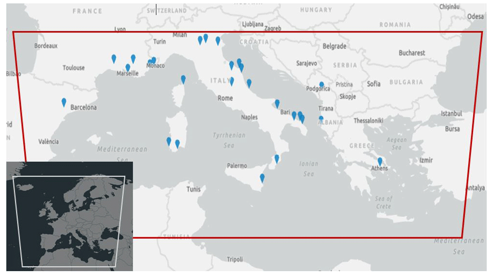
Figure A1Domains and measurement stations. The red trapezoid displays the 12×12 km2 domain, the blue icons are the locations of the measurement stations. On the bottom left the larger 36×36 km2 domain is displayed. Map source: ArcGIS Pro 2.7.1, Esri (2020).
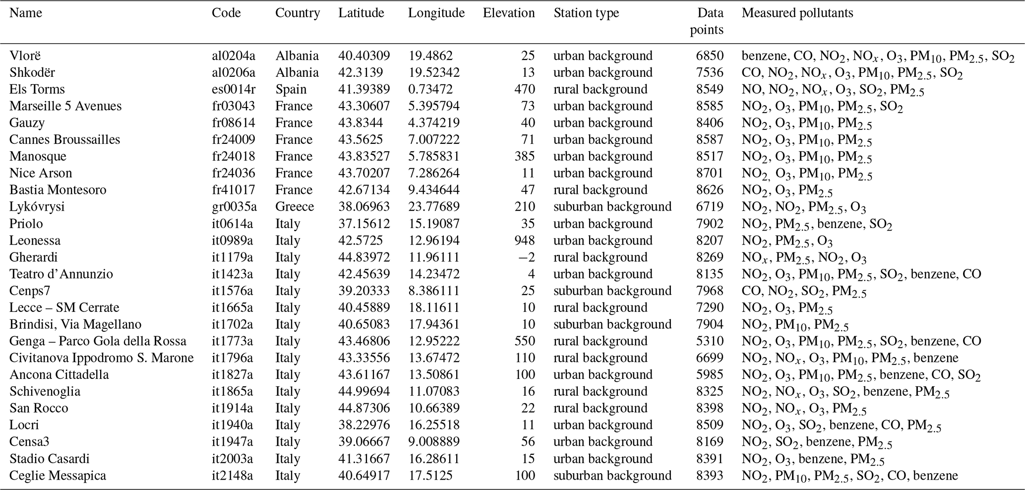
CAMx source code and documentation can be downloaded from https://camx-wp.azurewebsites.net/download/source/ (Ramboll Environment and Health, 2018) and the Chimere website (https://www.lmd.polytechnique.fr/chimere/2020_getcode.php, Cholakian et al., 2023). CMAQ version 5.2, which was used here, is available at https://doi.org/10.5281/zenodo.1167892 (US EPA Office of Research and Development, 2017). EMEP is available at https://doi.org/10.5281/zenodo.3647990 (EMEP MSC-W, 2020), LOTOS-EUROS is available at https://lotos-euros.tno.nl/open-source-version/ (Schaap et al., 2005), and WPS/WRF is available from the WPS (2023; https://github.com/wrf-model/WPS) and UCAR/NCAR Earth System Laboratory (2023, https://doi.org/10.5065/D6MK6B4K). The COSMO software is available at https://www.cosmo-model.org/content/support/software/default.htm#models (COSMO, 2023) and ecmwf-ifs/ifs-scripts at https://github.com/ecmwf-ifs (ECMWF IFS, 2023).
Data on measurement stations from EEA can be downloaded at https://discomap.eea.europa.eu/map/fme/AirQualityExport.htm (European Environment Agency, 2023). CTM model results are available upon request.
The supplement related to this article is available online at: https://doi.org/10.5194/acp-23-10163-2023-supplement.
LF: CMAQ model runs, evaluation and analysis of model results, preparation and writing of the paper. MK: analysis of the results, revision of the text. VM: supervision, analysis of the results, revision of the text. SO: CAMx and CHIMERE model runs, discussion of the results. RK and JK: LOTOS-EUROS model runs, land-based emissions data provision, discussion of the results. JM and SJ: EMEP model runs, discussion of the results. JPJ and EM: STEAM model runs, shipping emissions data provision, discussion of the results.
The contact author has declared that none of the authors has any competing interests.
Publisher’s note: Copernicus Publications remains neutral with regard to jurisdictional claims in published maps and institutional affiliations.
AtmoSud acknowledges the continuous support of CAMx by RAMBOLL and CHIMERE by LMD.
The Community Multiscale Air Quality (CMAQ) modeling system is developed and maintained by the US EPA. Its use is gratefully acknowledged. Ronny Petrik from Helmholtz-Zentrum Hereon (now at Marinekommando Deutsche Marine, Rostock) is acknowledged for providing meteorology and boundary conditions for the CMAQ runs.
The support from the Meteorological Synthesizing Center – West of EMEP at the Norwegian Meteorological Institute, especially from Peter Wind and David Simpson, in the implementation of emissions and meteorological fields used in this paper into the open-source EMEP model is gratefully acknowledged.
This research has been supported by the Horizon 2020 (grant no. 814893) program. The computations for the regional modeling using the EMEP model was enabled
by resources provided by the Swedish National Infrastructure for Computing
(SNIC), partially funded by the Swedish Research Council through grant
agreement no. 2018-05973.
The article processing charges for this open-access publication were covered by the Helmholtz-Zentrum Hereon.
This paper was edited by Fangqun Yu and reviewed by two anonymous referees.
Agrawal, H., Welch, W. A., Miller, J. W., and Cockert, D. R.: Emission measurements from a crude oil tanker at sea, Environ. Sci. Technol., 42, 7098–7103, https://doi.org/10.1021/es703102y, 2008.
Agrawal, H., Eden, R., Zhang, X., Fine, P. M., Katzenstein, A., Miller, J. W., Ospital, J., Teffera, S., and Cocker, D. R.: Primary particulate matter from ocean-going engines in the Southern California Air Basin, Environ. Sci. Technol., 43, 5398–5402, https://doi.org/10.1021/es8035016, 2009.
Agrawal, H., Welch, W. A., Henningsen, S., Miller, J. W., and Cocker, D. R.: Emissions from main propulsion engine on container ship at sea, J. Geophys. Res, 115, D23205, https://doi.org/10.1029/2009JD013346, 2010.
Aksoyoglu, S., Baltensperger, U., and Prévôt, A. S. H.: Contribution of ship emissions to the concentration and deposition of air pollutants in Europe, Atmos. Chem. Phys., 16, 1895–1906, https://doi.org/10.5194/acp-16-1895-2016, 2016.
Alfaro, S. D. and Gomes, L.: Modeling mineral aerosol production by wind erosion: Emission intensities and aerosol size distributions in source areas., J. Geophys. Res., 106, 18075–18084, https://doi.org/10.1029/2000jd900339, 2001.
Appel, K. W., Napelenok, S. L., Foley, K. M., Pye, H. O. T., Hogrefe, C., Luecken, D. J., Bash, J. O., Roselle, S. J., Pleim, J. E., Foroutan, H., Hutzell, W. T., Pouliot, G. A., Sarwar, G., Fahey, K. M., Gantt, B., Gilliam, R. C., Heath, N. K., Kang, D., Mathur, R., Schwede, D. B., Spero, T. L., Wong, D. C., and Young, J. O.: Description and evaluation of the Community Multiscale Air Quality (CMAQ) modeling system version 5.1, Geosci. Model Dev., 10, 1703–1732, https://doi.org/10.5194/gmd-10-1703-2017, 2017.
Astitha, M., Lelieveld, J., Abdel Kader, M., Pozzer, A., and de Meij, A.: Parameterization of dust emissions in the global atmospheric chemistry-climate model EMAC: impact of nudging and soil properties, Atmos. Chem. Phys., 12, 11057–11083, https://doi.org/10.5194/acp-12-11057-2012, 2012.
Baldasano, J. M., Pay, M. T., Jorba, O., Gassó, S., and Jiménez-Guerrero, P.: An annual assessment of air quality with the CALIOPE modeling system over Spain, Sci. Total Environ., 409, 2163–2178, https://doi.org/10.1016/j.scitotenv.2011.01.041, 2011.
Banzhaf, S., Schaap, M., Kerschbaumer, A., Reimer, E., Stern, R., van der Swaluw, E., and Builtjes, P.: Implementation and evaluation of pH-dependent cloud chemistry and wet deposition in the chemical transport model REM-Calgrid, Atmos. Environ., 49, 378–390, https://doi.org/10.1016/j.atmosenv.2011.10.069, 2012.
Barbu, A. L., Segers, A. J., Schaap, M., Heemink, A. W., and Builtjes, P. J. H.: A multi-component data assimilation experiment directed to sulphur dioxide and sulphate over Europe, Atmos. Environ., 43, 1622–1631, https://doi.org/10.1016/j.atmosenv.2008.12.005, 2009.
Behera, S. N., Sharma, M., Aneja, V. P., and Balasubramanian, R.: Ammonia in the atmosphere: a review on emission sources, atmospheric chemistry and deposition on terrestrial bodies, Environ Sci. Pollut. R., 20, 8092–8131, https://doi.org/10.1007/s11356-013-2051-9, 2013.
Berge, E. and Jakobsen, H. A.: A regional scale multilayer model for the calculation of long-term transport and deposition of air pollution in Europe, Tellus B, 50, 205–223, https://doi.org/10.3402/tellusb.v50i3.16097, 1998.
Bergström, R., Denier van der Gon, H. A. C., Prévôt, A. S. H., Yttri, K. E., and Simpson, D.: Modelling of organic aerosols over Europe (2002–2007) using a volatility basis set (VBS) framework: application of different assumptions regarding the formation of secondary organic aerosol, Atmos. Chem. Phys., 12, 8499–8527, https://doi.org/10.5194/acp-12-8499-2012, 2012.
Bieser, J., Aulinger, A., Matthias, V., Quante, M., and van der Denier Gon, H. A. C.: Vertical emission profiles for Europe based on plume rise calculations, Environ. Pollut., 159, 2935–2946, https://doi.org/10.1016/j.envpol.2011.04.030, 2011.
Binkowski, F. S. and Shankar, U.: The Regional Particulate Matter Model: 1. Model description and preliminary results, J. Geophys. Res., 100, 26191–26209, https://doi.org/10.1029/95JD02093, 1995.
Binkowski, F. S. and Roselle, S. J.: Models-3 Community Multiscale Air Quality (CMAQ) model aerosol component 1. Model description, J. Geophys. Res., 108, 4183, https://doi.org/10.1029/2001JD001409, 2003.
Byun, D. and Schere, K. L.: Review of the Governing Equations, Computational Algorithms, and Other Components of the Models-3 Community Multiscale Air Quality (CMAQ) Modeling System, Appl. Mech. Rev., 2, 51–77, https://doi.org/10.1115/1.2128636, 2006.
Carlton, A. G., Bhave, P. V., Napelenok, S. L., Edney, E. O., Sarwar, G., Pinder, R. W., Pouliot, G. A., and Houyoux, M.: Model representation of secondary organic aerosol in CMAQv4.7, Appl. Mech. Rev., 59, 51–77, https://doi.org/10.1021/es100636q, 2010.
Celik, S., Drewnick, F., Fachinger, F., Brooks, J., Darbyshire, E., Coe, H., Paris, J.-D., Eger, P. G., Schuladen, J., Tadic, I., Friedrich, N., Dienhart, D., Hottmann, B., Fischer, H., Crowley, J. N., Harder, H., and Borrmann, S.: Influence of vessel characteristics and atmospheric processes on the gas and particle phase of ship emission plumes: in situ measurements in the Mediterranean Sea and around the Arabian Peninsula, Atmos. Chem. Phys., 20, 4713–4734, https://doi.org/10.5194/acp-20-4713-2020, 2020.
Chen, R., Hu, B., Liu, Y., Xu, J., Yang, G., Xu, D., and Chen, C.: Beyond PM2.5: The role of ultrafine particles on adverse health effects of air pollution, Biochim. Biophys. Acta, 1860, 2844–2855, https://doi.org/10.1016/j.bbagen.2016.03.019, 2016.
Cholakian, A., Mailler, S., Pennel, R., Valari, M., Couvidat, F., Menut, L., and Siour, G.: CHIMERE v2020r3 version (+ WRF 3.7.1 + OASIS-MCT3), model code, https://www.lmd.polytechnique.fr/chimere/2020_getcode.php, last access: 19 January 2023.
Clappier, A., Thunis, P., Beekmann, M., Putaud, J. P., and Meij, A. de: Impact of SOx, NOx and NH3 emission reductions on PM2.5 concentrations across Europe: Hints for future measure development, Environ. Int., 156, 106699, https://doi.org/10.1016/j.envint.2021.106699, 2021.
Corbett, J. J. and Fischbeck, P.: Emissions from ships, Science, 278, 5339, 823–824, 1997.
COSMO Consortium: Models Supported by COSMO, COSMO [model], https://www.cosmo-model.org/content/support/software/default.htm#models, last access: 7 September 2023.
Donahue, N. M., Robinson, A. L., and Pandis, S. N.: Atmospheric organic particulate matter: From smoke to secondary organic aerosol, Atmos. Environ., 43, 94–106, https://doi.org/10.1016/j.atmosenv.2008.09.055, 2009.
Donateo, A., Gregoris, E., Gambaro, A., Merico, E., Giua, R., Nocioni, A., and Contini, D.: Contribution of harbour activities and ship traffic to PM2.5, particle number concentrations and PAHs in a port city of the Mediterranean Sea (Italy), Environ. Sci. Pollut. R., 21, 9415–9429, https://doi.org/10.1007/s11356-014-2849-0, 2014.
ECMWF IFS: ERA-Interim Reanalysis Data, GitHub [data set, code], https://github.com/ecmwf-ifs/era-interim (last access: 7 September 2023), 2023.
Emberson, L. D., Simpson, D., Tuovinen, J.-P., Ashmore, M. R. and Cambridge, H. M.: Towards a Model of Ozone Deposition and Stomatal Uptake over Europe, EMEP/MSC-W Note 6/00, Norwegian Meteorological Institute, Oslo, 57, 2000.
EMEP MSC-W.: metno/emep-ctm: OpenSource rv4.34 (202001) (rv4_34), Zenodo [model code], https://doi.org/10.5281/zenodo.3647990, 2020.
EMEP Status Report 1/2022: Transboundary particulate matter, photo-oxidants, acidifying and eutrophying components, Joint MSC-W & CCC & CEIP & CIAM Report, https://emep.int/publ/reports/2022/EMEP_Status_Report_1_2022.pdf (last access: 7 September 2023), 2022.
Erisman, J. W., van Pul, A., and Wyers, P.: Parametrization of surface resistance for the quantification of atmospheric deposition of acidifying pollutants and ozone, Atmos. Environ., 28, 2595–2607, https://doi.org/10.1016/1352-2310(94)90433-2, 1994.
Esri: ArcGIS Pro 2.7.1, Esri, https://www.esri.com/en-us/arcgis/products/arcgis-pro/overview (last access: 7 September 2023), 2020.
EU DIRECTIVE 2008/50/EC: European parliament: Directive 2008/50/EC of the European Parliament and of the Council of 21 May 2008 on ambient air quality and cleaner air for Europe, http://data.europa.eu/eli/dir/2008/50/oj (last access: 6 September 2023), 2008.
European Environment Agency: Air Quality Data Download Service, Discomap, European Environment Agency [data set], https://discomap.eea.europa.eu/map/fme/AirQualityExport.htm (last access: 7 September 2023), 2023.
Eyring, V.: Emissions from international shipping: 1. The last 50 years, J. Geophys. Res., 110, D17305, https://doi.org/10.1029/2004JD005619, 2005.
Eyring, V., Stevenson, D. S., Lauer, A., Dentener, F. J., Butler, T., Collins, W. J., Ellingsen, K., Gauss, M., Hauglustaine, D. A., Isaksen, I. S. A., Lawrence, M. G., Richter, A., Rodriguez, J. M., Sanderson, M., Strahan, S. E., Sudo, K., Szopa, S., van Noije, T. P. C., and Wild, O.: Multi-model simulations of the impact of international shipping on Atmospheric Chemistry and Climate in 2000 and 2030, Atmos. Chem. Phys., 7, 757–780, https://doi.org/10.5194/acp-7-757-2007, 2007.
Fécan, F., Marticorena, B., and Bergametti, G.: Parametrization of the increase of the aeolian erosion threshold wind friction velocity due to soil moisture for arid and semi-arid areas, Ann. Geophys., 17, 149–157, https://doi.org/10.1007/s00585-999-0149-7, 1999.
Fink, L., Karl, M., Matthias, V., Oppo, S., Kranenburg, R., Kuenen, J., Moldanova, J., Jutterström, S., Jalkanen, J.-P., and Majamäki, E.: Potential impact of shipping on air pollution in the Mediterranean region – a multimodel evaluation: comparison of photooxidants NO2 and O3, Atmos. Chem. Phys., 23, 1825–1862, https://doi.org/10.5194/acp-23-1825-2023, 2023.
Folberth, G. A., Hauglustaine, D. A., Lathière, J., and Brocheton, F.: Interactive chemistry in the Laboratoire de Météorologie Dynamique general circulation model: model description and impact analysis of biogenic hydrocarbons on tropospheric chemistry, Atmos. Chem. Phys., 6, 2273–2319, https://doi.org/10.5194/acp-6-2273-2006, 2006.
Foley, K. M., Roselle, S. J., Appel, K. W., Bhave, P. V., Pleim, J. E., Otte, T. L., Mathur, R., Sarwar, G., Young, J. O., Gilliam, R. C., Nolte, C. G., Kelly, J. T., Gilliland, A. B., and Bash, J. O.: Incremental testing of the Community Multiscale Air Quality (CMAQ) modeling system version 4.7, Geosci. Model Dev., 3, 205–226, https://doi.org/10.5194/gmd-3-205-2010, 2010.
Fountoukis, C. and Nenes, A.: ISORROPIA II: a computationally efficient thermodynamic equilibrium model for K+–Ca2+–Mg2+–NH–Na+–SO–NO–Cl−–H2O aerosols, Atmos. Chem. Phys., 7, 4639–4659, https://doi.org/10.5194/acp-7-4639-2007, 2007.
Friedrich, N., Eger, P., Shenolikar, J., Sobanski, N., Schuladen, J., Dienhart, D., Hottmann, B., Tadic, I., Fischer, H., Martinez, M., Rohloff, R., Tauer, S., Harder, H., Pfannerstill, E. Y., Wang, N., Williams, J., Brooks, J., Drewnick, F., Su, H., Li, G., Cheng, Y., Lelieveld, J., and Crowley, J. N.: Reactive nitrogen around the Arabian Peninsula and in the Mediterranean Sea during the 2017 AQABA ship campaign, Atmos. Chem. Phys., 21, 7473–7498, https://doi.org/10.5194/acp-21-7473-2021, 2021.
Gao, R. and Sang, N.: Quasi-ultrafine particles promote cell metastasis via HMGB1-mediated cancer cell adhesion, Environ. Pollut., 256, 113390, https://doi.org/10.1016/j.envpol.2019.113390, 2020.
Gašparac, G., Jeričević, A., Kumar, P., and Grisogono, B.: Regional-scale modelling for the assessment of atmospheric particulate matter concentrations at rural background locations in Europe, Atmos. Chem. Phys., 20, 6395–6415, https://doi.org/10.5194/acp-20-6395-2020, 2020.
Ge, Y., Heal, M. R., Stevenson, D. S., Wind, P., and Vieno, M.: Evaluation of global EMEP MSC-W (rv4.34) WRF (v3.9.1.1) model surface concentrations and wet deposition of reactive N and S with measurements, Geosci. Model Dev., 14, 7021–7046, https://doi.org/10.5194/gmd-14-7021-2021, 2021.
Ginoux, P., Chin, M., Tegen, I., Prospero, J. M., Holben, B., Dubovik, O., and Lin, S.-J.: Sources and distributions of dust aerosols simulated with the GOCART model, J. Geophys. Res., 106, 20255–20273, https://doi.org/10.1029/2000JD000053, 2001.
Gomes, L., Rajot, J. L., Alfaro, S. C., and Gaudichet, A.: Validation of a dust production model from measurements performed in semi-arid agricultural areas of Spain and Niger, Catena, 52, 257–271, 2003.
Granier, C., Darras, S., van der Denier Gon, H., Doubalova, J., Elguindi, N., Galle, B., Gauss, M., Guevara, M., Jalkanen, J.-P., Kuenen, J., Liousse, C., Quack, B., Simpson, D., and Sindelarova, K.: The Copernicus Atmosphere Monitoring Service global and regional emissions: (April 2019 version), Copernicus Atmosphere Monitoring Service (CAMS) report, https://doi.org/10.24380/d0bn-kx16, 2019.
Guenther, A., Zimmerman, P., Harley, P., Monson, R., and Fall, R.: Isoprene and monoterpene rate variability: model evaluations and sensitivity analyses, J. Geophys. Res., 98, 12609–12617, https://doi.org/10.1029/93JD00527, 1993.
Guenther, A., Hewitt, C., Erickson, D., Fall, R., Geron, C., Graedel, T., Harley, P., Klinger, L., Lerdau, M., McKay, W., Pierce, T., Scholes, R., Steinbrecher, R., Tallamraju, R., Taylor, J., and Zimmerman, P.: A global model of natural volatile organic compound emissions, J. Geophys. Res., 100, 8873–8892, https://doi.org/10.1029/94JD02950, 1995.
Hauglustaine, D. A., Balkanski, Y., and Schulz, M.: A global model simulation of present and future nitrate aerosols and their direct radiative forcing of climate, Atmos. Chem. Phys., 14, 11031–11063, https://doi.org/10.5194/acp-14-11031-2014, 2014.
Henzing, J. S., Olivié, D. J. L., and van Velthoven, P. F. J.: A parameterization of size resolved below cloud scavenging of aerosols by rain, Atmos. Chem. Phys., 6, 3363–3375, https://doi.org/10.5194/acp-6-3363-2006, 2006.
Heusinkveld, H. J., Wahle, T., Campbell, A., Westerink, R. H. S., Tran, L., Johnston, H., Stone, V., Cassee, F. R., and Schins, R. P. F.: Neurodegenerative and neurological disorders by small inhaled particles, NeuroToxicology, 56, 94–106, https://doi.org/10.1016/j.neuro.2016.07.007, 2016.
Im, U., Bianconi, R., Solazzo, E., Kioutsioukis, I., Badia, A., Balzarini, A., Baró, R., Bellasio, R., Brunner, D., Chemel, C., Curci, G., van der Denier Gon, H., Flemming, J., Forkel, R., Giordano, L., Jiménez-Guerrero, P., Hirtl, M., Hodzic, A., Honzak, L., Jorba, O., Knote, C., Makar, P. A., Manders-Groot, A., Neal, L., Pérez, J. L., Pirovano, G., Pouliot, G., San Jose, R., Savage, N., Schroder, W., Sokhi, R. S., Syrakov, D., Torian, A., Tuccella, P., Wang, K., Werhahn, J., Wolke, R., Zabkar, R., Zhang, Y., Zhang, J., Hogrefe, C., and Galmarini, S.: Evaluation of operational online-coupled regional air quality models over Europe and North America in the context of AQMEII phase 2. Part II: Particulate matter, Atmos. Environ. 17, 421–441, https://doi.org/10.1016/j.atmosenv.2014.08.072, 2014.
Im, U., Bianconi, R., Solazzo, E., Kioutsioukis, I., Badia, A., Balzarini, A., Baró, R., Bellasio, R., Brunner, D., Chemel, C., Curci, G., van der Denier Gon, H., Flemming, J., Forkel, R., Giordano, L., Jiménez-Guerrero, P., Hirtl, M., Hodzic, A., Honzak, L., Jorba, O., Knote, C., Makar, P. A., Manders-Groot, A., Neal, L., Pérez, J. L., Pirovano, G., Pouliot, G., San Jose, R., Savage, N., Schroder, W., Sokhi, R. S., Syrakov, D., Torian, A., Tuccella, P., Wang, K., Werhahn, J., Wolke, R., Zabkar, R., Zhang, Y., Zhang, J., Hogrefe, C., and Galmarini, S.: Evaluation of operational online-coupled regional air quality models over Europe and North America in the context of AQMEII phase 2. Part II: Particulate matter, Atmos. Environ., 115, 421–441, https://doi.org/10.1016/j.atmosenv.2014.08.072, 2015.
IMO (International Maritime Organization): Marine Environment Protection Committee (MEPC) – 79th session, 12–16 December 2022, https://www.imo.org/en/MediaCentre/MeetingSummaries/Pages/MEPC-79th-session.aspx (last access: 16 January 2023), 2022.
Jägerbrand, A. K., Brutemark, A., Barthel Svedén, J., and Gren, I.-M.: A review on the environmental impacts of shipping on aquatic and nearshore ecosystems, Sci. Total Environ., 695, 133637, https://doi.org/10.1016/j.scitotenv.2019.133637, 2019.
Jalkanen, J.-P., Brink, A., Kalli, J., Pettersson, H., Kukkonen, J., and Stipa, T.: A modelling system for the exhaust emissions of marine traffic and its application in the Baltic Sea area, Atmos. Chem. Phys., 9, 9209–9223, https://doi.org/10.5194/acp-9-9209-2009, 2009.
Jalkanen, J.-P., Johansson, L., Kukkonen, J., Brink, A., Kalli, J., and Stipa, T.: Extension of an assessment model of ship traffic exhaust emissions for particulate matter and carbon monoxide, Atmos. Chem. Phys., 12, 2641–2659, https://doi.org/10.5194/acp-12-2641-2012, 2012.
Johansson, L., Jalkanen, J.-P., Kalli, J., and Kukkonen, J.: The evolution of shipping emissions and the costs of regulation changes in the northern EU area, Atmos. Chem. Phys., 13, 11375–11389, https://doi.org/10.5194/acp-13-11375-2013, 2013.
Johansson, L., Jalkanen, J.-P., and Kukkonen, J.: Global assessment of shipping emissions in 2015 on a high spatial and temporal resolution, Atmos. Environ., 167, 403–415, https://doi.org/10.1016/j.atmosenv.2017.08.042, 2017.
Jiang, W., Smyth, S., Giroux, É., Roth, H., and Yin, D.: Differences between CMAQ fine mode particle and PM2.5 concentrations and their impact on model performance evaluation in the lower Fraser valley, Atmos. Environ., 40, 4973–4985, https://doi.org/10.1016/j.atmosenv.2005.10.069, 2006.
Jimenez, J. L., Canagaratna, M. R., Donahue, N. M., Prevot, A. S. H., Zhang, Q., Kroll, J. H., DeCarlo, P. F., Allan, J. D., Coe, H., Ng, N. L., Aiken, A. C., Docherty, K. S., Ulbrich, I. M., Grieshop, A. P., Robinson, A. L., Duplissy, J., Smith, J. D., Wilson, K. R., Lanz, V. A., Hueglin, C., Sun, Y. L., Tian, J., Laaksonen, A., Raatikainen, T., Rautiainen, J., Vaattovaara, P., Ehn, M., Kulmala, M., Tomlinson, J. M., Collins, D. R., Cubison, M. J., Dunlea, E. J., Huffman, J. A., Onasch, T. B., Alfarra, M. R., Williams, P. I., Bower, K., Kondo, Y., Schneider, J., Drewnick, F., Borrmann, S., Weimer, S., Demerjian, K., Salcedo, D., Cottrell, L., Griffin, R., Takami, A., Miyoshi, T., Hatakeyama, S., Shimono, A., Sun, J. Y., Zhang, Y. M., Dzepina, K., Kimmel, J. R., Sueper, D., Jayne, J. T., Herndon, S. C., Trimborn, A. M., Williams, L. R., Wood, E. C., Middlebrook, A. M., Kolb, C. E., Baltensperger, U., and Worsnop, D. R.: Evolution of organic aerosols in the atmosphere, Science, 326, 1525–1529, https://doi.org/10.1126/science.1180353, 2009.
Jonson, J. E., Gauss, M., Schulz, M., Jalkanen, J.-P., and Fagerli, H.: Effects of global ship emissions on European air pollution levels, Atmos. Chem. Phys., 20, 11399–11422, https://doi.org/10.5194/acp-20-11399-2020, 2020.
Karamfilova, E.: BRIEFING Implementation Appraisal, Revision of the EU Ambient Air Quality Directives, EPRS European Parliamentary Research Service, https://www.europarl.europa.eu/RegData/etudes/BRIE/2022/734679/EPRS_BRI(2022)734679_EN.pdf (last access: 7 September 2023), 2022.
Karl, M., Bieser, J., Geyer, B., Matthias, V., Jalkanen, J.-P., Johansson, L., and Fridell, E.: Impact of a nitrogen emission control area (NECA) on the future air quality and nitrogen deposition to seawater in the Baltic Sea region, Atmos. Chem. Phys., 19, 1721–1752, https://doi.org/10.5194/acp-19-1721-2019, 2019.
Kelly, J. T., Bhave, P. V., Nolte, C. G., Shankar, U., and Foley, K. M.: Simulating emission and chemical evolution of coarse sea-salt particles in the Community Multiscale Air Quality (CMAQ) model, Geosci. Model Dev., 3, 257–273, https://doi.org/10.5194/gmd-3-257-2010, 2010.
Kiesewetter, G., Schoepp, W., Heyes, C., and Amann, M.: Modelling PM2.5 impact indicators in Europe: Health effects and legal compliance, Environ. Modell Softw., 74, 201–211, https://doi.org/10.1016/j.envsoft.2015.02.022, 2015.
Klingmüller, K., Metzger, S., Abdelkader, M., Karydis, V. A., Stenchikov, G. L., Pozzer, A., and Lelieveld, J.: Revised mineral dust emissions in the atmospheric chemistry–climate model EMAC (MESSy 2.52 DU_Astitha1 KKDU2017 patch), Geosci. Model Dev., 11, 989–1008, https://doi.org/10.5194/gmd-11-989-2018, 2018.
Kleijn, D., Kohler, F., Báldi, A., Batáry, P., Concepción, E. D., Clough, Y., Díaz, M., Gabriel, D., Holzschuh, A., Knop, E., Kovács, A., Marshall, E. J. P., Tscharntke, T., and Verhulst, J.: On the relationship between farmland biodiversity and land-use intensity in Europe, P. R. Soc., 276, 1658, https://doi.org/10.1098/rspb.2008.1509, 2009.
Klimont, Z., Kupiainen, K., Heyes, C., Purohit, P., Cofala, J., Rafaj, P., Borken-Kleefeld, J., and Schöpp, W.: Global anthropogenic emissions of particulate matter including black carbon, Atmos. Chem. Phys., 17, 8681–8723, https://doi.org/10.5194/acp-17-8681-2017, 2017.
Kranenburg, R., Segers, A. J., Hendriks, C., and Schaap, M.: Source apportionment using LOTOS-EUROS: module description and evaluation, Geosci. Model Dev., 6, 721–733, https://doi.org/10.5194/gmd-6-721-2013, 2013.
Krupa, S. V.: Effects of atmospheric ammonia (NH3) on terrestrial vegetation: a review, Environ. Pollut., 124, 179–221, https://doi.org/10.1016/s0269-7491(02)00434-7, 2003.
Kuenen, J., Dellaert, S., Visschedijk, A., Jalkanen, J.-P., Super, I., and Denier van der Gon, H.: CAMS-REG-v4: a state-of-the-art high-resolution European emission inventory for air quality modelling, Earth Syst. Sci. Data, 14, 491–515, https://doi.org/10.5194/essd-14-491-2022, 2022.
Kuenen, J. J. P., Visschedijk, A. J. H., Jozwicka, M., and Denier van der Gon, H. A. C.: TNO-MACC_II emission inventory; a multi-year (2003–2009) consistent high-resolution European emission inventory for air quality modelling, Atmos. Chem. Phys., 14, 10963–10976, https://doi.org/10.5194/acp-14-10963-2014, 2014.
Loosmore, G. A. and Cederwall, R. T.: Precipitation scavenging of atmospheric aerosols for emergency response applications: testing an updated model with new real-time data, Atmos. Environ., 38, 993–1003, https://doi.org/10.1016/j.atmosenv.2003.10.055, 2004.
Mallet, M. D., D'Anna, B., Même, A., Bove, M. C., Cassola, F., Pace, G., Desboeufs, K., Di Biagio, C., Doussin, J.-F., Maille, M., Massabò, D., Sciare, J., Zapf, P., di Sarra, A. G., and Formenti, P.: Summertime surface PM1 aerosol composition and size by source region at the Lampedusa island in the central Mediterranean Sea, Atmos. Chem. Phys., 19, 11123–11142, https://doi.org/10.5194/acp-19-11123-2019, 2019.
Manders, A. M. M., Builtjes, P. J. H., Curier, L., Denier van der Gon, H. A. C., Hendriks, C., Jonkers, S., Kranenburg, R., Kuenen, J. J. P., Segers, A. J., Timmermans, R. M. A., Visschedijk, A. J. H., Wichink Kruit, R. J., van Pul, W. A. J., Sauter, F. J., van der Swaluw, E., Swart, D. P. J., Douros, J., Eskes, H., van Meijgaard, E., van Ulft, B., van Velthoven, P., Banzhaf, S., Mues, A. C., Stern, R., Fu, G., Lu, S., Heemink, A., van Velzen, N., and Schaap, M.: Curriculum vitae of the LOTOS–EUROS (v2.0) chemistry transport model, Geosci. Model Dev., 10, 4145–4173, https://doi.org/10.5194/gmd-10-4145-2017, 2017.
Manders-Groot, A., Segers, A., and Jonkers, S.: LOTOS-EUROS v2.0 Reference Guide, Report, https://airqualitymodeling.tno.nl/publish/pages/3175/lotos-euros-reference-guide.pdf (last access: 7 September 2023), 2016.
Marmer, E. and Langmann, B.: Impact of ship emissions on the Mediterranean summertime pollution and climate: A regional model study, Atmos. Environ., 39, 4659–4669, https://doi.org/10.1016/j.atmosenv.2005.04.014, 2005.
Mårtensson, E. M., Nilsson, E. D., Leeuw, G. de, Cohen, L. H., and Hansson, H.-C.: Laboratory simulations and parameterization of the primary marine aerosol production, J. Geophys. Res., 108, 4297, https://doi.org/10.1029/2002JD002263, 2003.
Marticorena, B. and Bergametti, G.: Modelling the atmospheric dust cycle: 1. Design of a soil drived dust emission scheme., J. Geophys. Res., 100, 16415–16430, https://doi.org/10.1029/95jd00690, 1995.
Marticorena, B., Bergametti, G., Aumont, B., Callot, Y., N'Doumé, C., and Legrand, M.: Modelling the atmospheric dust cycle: 2. Simulation of Saharan dust sources, J. Geophys. Res., 102, 4387–4404, 1997.
Matthias, V.: The aerosol distribution in Europe derived with the Community Multiscale Air Quality (CMAQ) model: comparison to near surface in situ and sunphotometer measurements, Atmos. Chem. Phys., 8, 5077–5097, https://doi.org/10.5194/acp-8-5077-2008, 2008.
Matthias, V., Bewersdorff, I., Aulinger, A., and Quante, M.: The contribution of ship emissions to air pollution in the North Sea regions, Environ. Pollut., 158, 2241–2250, https://doi.org/10.1016/j.envpol.2010.02.013, 2010.
Menut, L., Bessagnet, B., Khvorostyanov, D., Beekmann, M., Blond, N., Colette, A., Coll, I., Curci, G., Foret, G., Hodzic, A., Mailler, S., Meleux, F., Monge, J.-L., Pison, I., Siour, G., Turquety, S., Valari, M., Vautard, R., and Vivanco, M. G.: CHIMERE 2013: a model for regional atmospheric composition modelling, Geosci. Model Dev., 6, 981–1028, https://doi.org/10.5194/gmd-6-981-2013, 2013.
Monahan, E. C., Spiel, D. E., and Davidson, K. L.: A Model of Marine Aerosol Generation Via Whitecaps and Wave Disruption, OCSL, 2, https://doi.org/10.1007/978-94-009-4668-2_16, 1986.
Nenes, A., Pandis, S. N., and Pilinis, C.: ISORROPIA: A New Thermodynamic Equilibrium Model for Multiphase Multicomponent Inorganic Aerosols, Aquat. Geochem., 4, 123–152, https://doi.org/10.1023/A:1009604003981, 1998.
Nunes, R. A. O., Alvim-Ferraz, M. C. M., Martins, F. G., Calderay-Cayetano, F., Durán-Grados, V., Moreno-Gutiérrez, J., Jalkanen, J.-P., Hannuniemi, H., and Sousa, S. I. V.: Shipping emissions in the Iberian Peninsula and the impacts on air quality, Atmos. Chem. Phys., 20, 9473–9489, https://doi.org/10.5194/acp-20-9473-2020, 2020.
Ovadnevaite, J., Manders, A., de Leeuw, G., Ceburnis, D., Monahan, C., Partanen, A.-I., Korhonen, H., and O'Dowd, C. D.: A sea spray aerosol flux parameterization encapsulating wave state, Atmos. Chem. Phys., 14, 1837–1852, https://doi.org/10.5194/acp-14-1837-2014, 2014.
Palacios-Peña, L., Lorente-Plazas, R., Montávez, J. P., and Jiménez-Guerrero, P.: Saharan Dust Modeling Over the Mediterranean Basin and Central Europe: Does the Resolution Matter?, Front. Earth Sci., 7, 290, https://doi.org/10.3389/feart.2019.00290, 2019.
Pandolfi, M., Gonzalez-Castanedo, Y., Alastuey, A., La Rosa, J. D. de, Mantilla, E., La Campa, A. S. de, Querol, X., Pey, J., Amato, F., and Moreno, T.: Source apportionment of PM10 and PM2.5 at multiple sites in the strait of Gibraltar by PMF: impact of shipping emissions, Environ. Sci. Pollut. R., 18, 260–269, https://doi.org/10.1007/s11356-010-0373-4, 2011.
Pepe, N., Pirovano, G., Balzarini, A., Toppetti, A., Riva, G. M., Amato, F., and Lonati, G.: Enhanced CAMx source apportionment analysis at an urban receptor in Milan based on source categories and emission regions, Atmos. Environ. X, 2, 100020, https://doi.org/10.1016/j.aeaoa.2019.100020, 2019.
Pleim, J. E., Xiu, A., Finkelstein, P. L., and Otte, T. L.: A Coupled Land-Surface and Dry Deposition Model and Comparison to Field Measurements of Surface Heat, Moisture, and Ozone Fluxes, Water Air Soil Poll.-Focus, 1, 243–252, https://doi.org/10.1023/A:1013123725860, 2001.
Prati, M. V., Costagliola, M. A., Quaranta, F., and Murena, F.: Assessment of ambient air quality in the port of Naples, J. Air Waste Manage., 65, 970–979, https://doi.org/10.1080/10962247.2015.1050129, 2015.
Pun, B. K., Seigneur, C., and Lohman, K.: Modeling secondary organic aerosol formation via multiphase partitioning with molecular data, Environ. Sci. Technol., 40, 4722–4731, https://doi.org/10.1021/es0522736, 2006.
Pye, H. O. T. and Pouliot, G. A.: Modeling the role of alkanes, polycyclic aromatic hydrocarbons, and their oligomers in secondary organic aerosol formation, Environ. Sci. Technol., 46, 6041–6047, https://doi.org/10.1021/es300409w, 2012.
Pye, H. O. T., Murphy, B. N., Xu, L., Ng, N. L., Carlton, A. G., Guo, H., Weber, R., Vasilakos, P., Appel, K. W., Budisulistiorini, S. H., Surratt, J. D., Nenes, A., Hu, W., Jimenez, J. L., Isaacman-VanWertz, G., Misztal, P. K., and Goldstein, A. H.: On the implications of aerosol liquid water and phase separation for organic aerosol mass, Atmos. Chem. Phys., 17, 343–369, https://doi.org/10.5194/acp-17-343-2017, 2017.
Ramboll Environment and Health: CAMx Source Code and Documentation, CAMx v6.50 (April 30, 2018), https://camx-wp.azurewebsites.net/download/source/ (last access: 7 September 2023), 2018.
Ramboll Environment and Health: User's Guide COMPREHENSIVE AIR QUALITY MODEL WITH EXTENSIONS: Version 7.10, User's Guide, https://camx-wp.azurewebsites.net/Files/CAMxUsersGuide_v7.10.pdf (last access: 7 September 2023), 2020.
Reichle, L. J., Cook, R., Yanca, C. A., and Sonntag, D. B.: Development of organic gas exhaust speciation profiles for nonroad spark-ignition and compression-ignition engines and equipment, J. Air Waste Manage., 65, 1185–1193, https://doi.org/10.1080/10962247.2015.1020118, 2015.
Remke, E., Brouwer, E., Kooijman, A., Blindow, I., Esselink, H., and Roelofs, J. G. M.: Even low to medium nitrogen deposition impacts vegetation of dry, coastal dunes around the Baltic Sea, Environ. Pollut., 157, 792–800, https://doi.org/10.1016/j.envpol.2008.11.020, 2009.
Riccio, A., Ciaramella, A., Giunta, G., Galmarini, S., Solazzo, E., and Potempski, S.: On the systematic reductionof data complexity in multimodel atmospheric dispersion ensemble modeling, J. Geophys. Res., 117, D05314, https://doi.org/10.1029/2011JD016503, 2012.
Robinson, A. L., Donahue, N. M., Shrivastava, M. K., Weitkamp, E. A., Sage, A. M., Grieshop, A. P., Lane, T. E., Pierce, J. R., and Pandis, S. N.: Rethinking organic aerosols: semivolatile emissions and photochemical aging, Science, 315, 1259—1262, https://doi.org/10.1126/science.1133061, 2007.
Roselle, S. J. and Binkowski, F. S.: Cloud Dynamics and Chemistry, Chap. 11, https://www.cmascenter.org/cmaq/science_documentation/pdf/ch11.pdf (last access: 7 September 2023), 1999.
Schaap, M., van Loon, M., ten Brink, H. M., Dentener, F. J., and Builtjes, P. J. H.: Secondary inorganic aerosol simulations for Europe with special attention to nitrate, Atmos. Chem. Phys., 4, 857–874, https://doi.org/10.5194/acp-4-857-2004, 2004.
Schaap, M., Sauter, F., Boersen, G., and Builtjes, P.: The integration of LOTOS and EUROS: Activities during 2004. Tech. rep. Apeldoorn, The Netherlands (in Dutch): TNOreport B&O-A R2005/209, 2005 (data available at: https://lotos-euros.tno.nl/open-source-version/, last access: 19 January 2023).
Schaap, M., Manders, A. M. M., Hendriks, E. C. J., Cnossen, J. M., Segers, A. J. S., Denier van der Gon, H. A. C., Jozwicka, M., Sauter, F., Velders, G., Matthijsen, J., and Builtjes, P. J. H.: Regional modelling of particulate matter for the Netherlands, Tech. rep., Netherlands Environmental Assessment Agency (PBL), https://www.pbl.nl/sites/default/files/downloads/500099008_0.pdf (last access: 7 September 2023), 2009.
Schembari, C., Cavalli, F., Cuccia, E., Hjorth, J., Calzolai, G., Pérez, N., Pey, J., Prati, P., and Raes, F.: Impact of a European directive on ship emissions on air quality in Mediterranean harbours, Atmos. Environ., 61, 661–669, https://doi.org/10.1016/j.atmosenv.2012.06.047, 2012.
Schober, P., Boer, C., and Schwarte, L. A.: Correlation Coefficients: Appropriate Use and Interpretation, Anesth. Analg., 126, 1763–1768, https://doi.org/10.1213/ANE.0000000000002864, 2018.
Seinfeld, J. H. and Pandis, S. N.: Atmospheric Chemistry and Physics, John Wiley and Sons, New York, ISBN 9781119221166, 1998.
Seinfeld, J. H. and Pandis, S. N.: Atmospheric Chemistry and Physics: From Air Pollution to Climate Change. 2nd Edition, John Wiley & Sons, New York, ISBN 978-1118947401, 2006.
Simpson, D., Benedictow, A., Berge, H., Bergström, R., Emberson, L. D., Fagerli, H., Flechard, C. R., Hayman, G. D., Gauss, M., Jonson, J. E., Jenkin, M. E., Nyíri, A., Richter, C., Semeena, V. S., Tsyro, S., Tuovinen, J.-P., Valdebenito, Á., and Wind, P.: The EMEP MSC-W chemical transport model – technical description, Atmos. Chem. Phys., 12, 7825–7865, https://doi.org/10.5194/acp-12-7825-2012, 2012.
Simpson, D., Bergström, R., Briolat, A., Imhof, H., Johansson, J., Priestley, M., and Valdebenito, A.: GenChem v1.0 – a chemical pre-processing and testing system for atmospheric modelling, Geosci. Model Dev., 13, 6447–6465, https://doi.org/10.5194/gmd-13-6447-2020, 2020.
Sippula, O., Stengel, B., Sklorz, M., Streibel, T., Rabe, R., Orasche, J., Lintelmann, J., Michalke, B., Abbaszade, G., Radischat, C., Gröger, T., Schnelle-Kreis, J., Harndorf, H., and Zimmermann, R.: Particle emissions from a marine engine: chemical composition and aromatic emission profiles under various operating conditions, Environ. Sci. Technol., 48, 11721–11729, https://doi.org/10.1021/es502484z, 2014.
Solazzo, E., Bianconi, R., Pirovano, G., Matthias, V., Vautard, R., Moran, M. D., Wyat Appel, K., Bessagnet, B., Brandt, J., Christensen, J. H., Chemel, C., Coll, I., Ferreira, J., Forkel, R., Francis, X. V., Grell, G., Grossi, P., Hansen, A. B., Miranda, A. I., Nopmongcol, U., Prank, M., Sartelet, K. N., Schaap, M., Silver, J. D., Sokhi, R. S., Vira, J., Werhahn, J., Wolke, R., Yarwood, G., Zhang, J., Rao, S. T., and Galmarini, S.: Operational model evaluation for particulate matter in Europe and North America in the context of AQMEII, Atmos. Environ., 53, 75–92, https://doi.org/10.1016/j.atmosenv.2012.02.045, 2012.
Solazzo, E., Riccio, A., Kioutsioukis, I., and Galmarini, S.: Pauci ex tanto numero: reduce redundancy in multi-model ensembles, Atmos. Chem. Phys., 13, 8315–8333, https://doi.org/10.5194/acp-13-8315-2013, 2013.
Solazzo, E., Riccio, A., van Dingenen, R., Valentini, L., and Galmarini, S.: Evaluation and uncertainty estimation of the impact of air quality modelling on crop yields and premature deaths using a multi-model ensemble, Sci. Total Environ., 633, 1437–1452, https://doi.org/10.1016/j.scitotenv.2018.03.317, 2018.
Song, S.-K. and Shon, Z.-H.: Current and future emission estimates of exhaust gases and particles from shipping at the largest port in Korea, Environ. Sci. Pollut. R., 21, 6612–6622, https://doi.org/10.1007/s11356-014-2569-5, 2014.
Sotiropoulou, R. E. P. and Tagaris, E.: Impact of Shipping Emissions on European Air Quality, in: Perspectives on Atmospheric Sciences, edited by: Karacostas, T., Bais, A., and Nastos, P., Springer Atmospheric Sciences, https://doi.org/10.1007/978-3-319-35095-0_149, 2017.
Strader, R., Lurmann, F., and Pandis, S. N.: Evaluation of secondary organic aerosol formation in winter, Atmos. Environ., 33, 4849–4863, https://doi.org/10.1016/S1352-2310(99)00310-6, 1999.
Tadic, I., Crowley, J. N., Dienhart, D., Eger, P., Harder, H., Hottmann, B., Martinez, M., Parchatka, U., Paris, J.-D., Pozzer, A., Rohloff, R., Schuladen, J., Shenolikar, J., Tauer, S., Lelieveld, J., and Fischer, H.: Net ozone production and its relationship to nitrogen oxides and volatile organic compounds in the marine boundary layer around the Arabian Peninsula, Atmos. Chem. Phys., 20, 6769–6787, https://doi.org/10.5194/acp-20-6769-2020, 2020.
Tomasi, C. and Lupi, A.: Primary and secondary sources of atmospheric aerosol, Atmospheric Aerosols: Life Cycles and Effects on Air Quality and Climate, Wiley, 1–86, https://doi.org/10.1002/9783527336449.ch1, 2017.
Tuccella, P., Menut, L., Briant, R., Deroubaix, A., Khvorostyanov, D., Mailler, S., Siour, G., and Turquety, S.: Implementation of Aerosol-Cloud Interaction within WRF-CHIMERE Online Coupled Model: Evaluation and Investigation of the Indirect Radiative Effect from Anthropogenic Emission Reduction on the Benelux Union, Atmosphere, 10, 20, https://doi.org/10.3390/atmos10010020, 2019.
UCAR/NCAR Earth System Laboratory: WRF – Weather Research and Forecasting Model Users' Page, MMM/WRF [model code], https://doi.org/10.5065/D6MK6B4K, 2023.
US EPA Office of Research and Development: CMAQ (5.2), Zenodo [model code], https://doi.org/10.5281/zenodo.1167892, 2017.
Večeřa, Z., Mikuška, P., Smolík, J., Eleftheriadis, K., Bryant, C., Colbeck, I., and Lazaridis, M.: Shipboard Measurements of Nitrogen Dioxide, Nitrous Acid, Nitric Acid and Ozone in the Eastern Mediterranean Sea, Water Air Soil Poll.-Focus, 8, 117–125, https://doi.org/10.1007/s11267-007-9133-y, 2008.
Viana, M., Amato, F., Alastuey, A., Querol, X., Moreno, T., Dos Santos, S. G., Herce, M. D., and Fernández-Patier, R.: Chemical tracers of particulate emissions from commercial shipping, Environ. Sci. Technol., 43, 7472–7477, https://doi.org/10.1021/es901558t, 2009.
Viana, M., Hammingh, P., Colette, A., Querol, X., Degraeuwe, B., Vlieger, I. d., and van Aardenne, J.: Impact of maritime transport emissions on coastal air quality in Europe, Atmos. Environ., 90, 96–105, https://doi.org/10.1016/j.atmosenv.2014.03.046, 2014.
Viana, M., Rizza, V., Tobías, A., Carr, E., Corbett, J., Sofiev, M., Karanasiou, A., Buonanno, G., and Fann, N.: Estimated health impacts from maritime transport in the Mediterranean region and benefits from the use of cleaner fuels, Environ. Internat., 138, 105670, https://doi.org/10.1016/j.envint.2020.105670, 2020.
Wesely, M. L.: Parameterization of surface resistances to gaseous dry deposition in regional-scale numerical models, Atmos. Environ., 23, 1293–1304, https://doi.org/10.1016/0004-6981(89)90153-4, 1989.
Whitten, G. Z., Hogo, H., and Killus, J. P.: The carbon-bond mechanism: A condensed kinetic mechanism for photochemical smog, Environ. Sci. Technol., 18, 280–287, 1980.
Wiedinmyer, C., Akagi, S. K., Yokelson, R. J., Emmons, L. K., Al-Saadi, J. A., Orlando, J. J., and Soja, A. J.: The Fire INventory from NCAR (FINN): a high resolution global model to estimate the emissions from open burning, Geosci. Model Dev., 4, 625–641, https://doi.org/10.5194/gmd-4-625-2011, 2011.
WPS: The Weather Research and Forecasting (WRF) Preprocessing System, GitHub [data set, code], https://github.com/wrf-model/WPS, last access: 7 September 2023.
Zender, C., Bian, H., and Newman, D.: Mineral Dust Entrainmentand Deposition (DEAD) model: Description and 1990s dust climatology, J. Geophys. Res., 108, 4416–4437, https://doi.org/10.1029/2002jd002775, 2003.
Zhang, L., Brook, J. R., and Vet, R.: A revised parameterization for gaseous dry deposition in air-quality models, Atmos. Chem. Phys., 3, 2067–2082, https://doi.org/10.5194/acp-3-2067-2003, 2003.
Zhong, Q., Shen, H., Yun, X., Chen, Y., Ren, Y.'a., Xu, H., Shen, G., Du, W., Meng, J., Li, W., Ma, J., and Tao, S.: Global Sulfur Dioxide Emissions and the Driving Forces, Environ. Sci. Technol., 54, 6508–6517, https://doi.org/10.1021/acs.est.9b07696, 2020.